Resource Allocation and Ine ciency in the Financial...

Resource Allocation and Inefficiency

in the Financial Sector∗

Kinda Hachem†

Chicago Booth and NBER

First Version November 2010; This Version July 2014

Abstract

I analyze whether banks are efficient at allocating resources across intermediation ac-tivities. Competition between lenders means that resources are needed to draw bor-rowers into credit matches. At the same time, imperfect information between lendersand borrowers means that resources are also needed for screening. I show that theprivately optimal allocation of resources is constrained inefficient. In particular, toomany resources are spent on getting rather than vetting borrowers but, once properlyvetted, not enough matches are retained. Uninformed lending is thus inefficiently high,informed lending is inefficiently low, and a tax on matching activities helps remedy thesituation. (JEL D62, D83, E44)

∗This paper is based on the second chapter of my dissertation at the University of Toronto. I thank JonS. Cohen, Doug Diamond, Miquel Faig, Pedro Gete, Alok Johri, Gueorgui Kambourov, Anil Kashyap, JimPesando, David Ross, Shouyong Shi, Andy Skrzypacz, and seminar participants at numerous institutionsand conferences for constructive comments. Financial support from Chicago Booth, the Social Sciencesand Humanities Research Council of Canada, and Shouyong Shi’s Bank of Canada Fellowship and CanadaResearch Chair are gratefully acknowledged. Any errors are my own.†University of Chicago, Booth School of Business, 5807 South Woodlawn Avenue, Chicago, IL 60637,

USA. Tel: 1-773-834-0229. Email: [email protected].

1

1 Introduction

Understanding how agents allocate finite resources is fundamental to economics yet very little

work exists on the allocation of bank resources across intermediation activities. Attracting

new clients is a competitive endeavor so we often observe banks creating financial products

and advertising their loan services (matching activities). At the same time, information

frictions such as adverse selection mean that banks must also devote some resources to

learning about who they attract (screening activities). A tradeoff arises because the marginal

resource put into one activity could have instead been put into the other. Do the private

and social margins line up? I show that they do not: lenders screen too little but are then

overly selective about who to finance once informed. These results contrast with existing

papers and have important implications for the health of the financial system.

Central to my analysis is that both matching and screening are costly. The literature on

adverse selection has traditionally bundled these activities and predicted that lenders screen

too much. Excessive screening, however, is difficult to reconcile with the run-up to the

recent financial crisis: by all accounts, information acquisition was low and economists have

turned to securitization for answers.1 While securitization can certainly distort incentives,

my results suggest it is not a prerequisite for too little screening: there are potentially deeper

problems in how competing banks allocate resources across intermediation activities.

To understand the mechanisms in my model, begin with the allocation decision of an

unmatched lender. By budgeting resources to both matching and screening, this lender forms

an informed match with positive probability. If the borrower is desirable, then the match

is retained and unavailable to other lenders until it breaks. If the borrower is undesirable,

then the match is rejected and the borrower returns to the available pool. An increase

in informed matching thus worsens the adverse selection problem faced by other lenders.

1The adverse selection literature is discussed in more detail at the end of this section. The negative effectof securitization on screening is shown empirically in Keys et al (2010) and Purnanandam (2011) but, asper Gorton and Pennacchi (1995) and subsequent work, originate-to-distribute models cannot completelyeliminate screening since loan sales must be incentive compatible.

2

The intuition behind too much screening in other papers is that more screening leads to

more informed matches. Resource allocation breaks this intuition by introducing a non-

monotonicity in the relationship between screening and the number of informed matches.

If lenders devote a tiny share of resources to screening, then few matches are informed

and the distribution of available borrowers is largely unchanged. An increase in screening

deteriorates the distribution by creating more informed matches but, as more and more

resources are funneled into screening, matching becomes very low and the deterioration

reverses: the fraction of informed matches is high but the number is low. Put another way,

more screening can sometimes produce a better distribution than less screening.

The non-monotonicity just described is the first step away from the conventional view

of too much screening. The second step is understanding how resource allocation affects

the retention decisions of informed lenders. To this end, consider two screening intensities

with the same effect on the distribution of available borrowers. Since the relationship be-

tween screening and the number of informed matches is non-monotone, we know that such

intensities exist. The higher of the two screening intensities leaves fewer resources open for

matching. This decreases the rate at which unmatched lenders contact the available distri-

bution, increasing the expected duration until a good draw. The value of being unmatched

then falls, prompting informed lenders to retain more of their matches. More screening can

thus have a positive effect on the survival of informed matches.

Key to the discussion so far is that lenders choose the cutoff between desirable and

undesirable borrowers once informed. This is a departure from banking models with two

borrower types. By assuming one good type and one bad type, such models make the

retention decision of an informed lender exogenous. With an exogenous cutoff, I show that

a Walrasian interbank market prices the effect of resource allocation on the distribution of

available borrowers. With an endogenous cutoff, however, one market cannot price both the

distributional externality and the additional effect on informed lenders. The result is too

little screening and too little informed retention.

3

By way of corrective taxation, I also show that a matching tax which remits proceeds

to the interbank market implements the constrained efficient allocation as an equilibrium.

In contrast, a broader scheme that taxes lender revenues is entirely ineffective. Absent a

matching tax, my model predicts that uninformed credit is inefficiently high and informed

credit is inefficiently low. Lenders as a whole thus recover too little from their borrowers and

the economy settles on a steady state that supports too little credit overall.

All of the results described so far are robust to the introduction of moral hazard. Indeed,

allowing lenders to influence borrower effort via loan rates increases the welfare loss stem-

ming from my externalities. The results are also robust to relationship lending under high

discount factors. Relationship lending allows lenders to learn about their borrowers through

repeated interactions.2 Therefore, even if initial screening is unsuccessful, a lender can dis-

cover his borrower’s type during the process of providing uninformed credit. On one hand,

this mitigates the downside of entering an uninformed match but, on the other, it worsens

the distribution of available borrowers. The discount factor governs how lenders weigh a

worse distribution against the fact that learning through relationship lending is a lagged

substitute for screening. I show that there is one discount factor for which the decentralized

economy with relationship lending achieves constrained efficiency. For discount factors above

this critical value, too little screening and too little informed retention re-emerge.

In emphasizing financial non-neutrality, my paper is broadly related to the macroe-

conomic literature on credit channels (e.g., Gurley and Shaw (1955), Williamson (1987),

Bernanke and Gertler (1989), Kiyotaki and Moore (1997)). It also relates to a recent branch

of this literature which investigates financial sector inefficiency under the asset price mech-

anism of Kiyotaki and Moore (1997). In Lorenzoni (2008) and Korinek (2011), for example,

firms do not internalize that more leverage will require more fire sales should a negative

shock hit. The result is over-borrowing ex ante and the potential for a financial crisis ex

post. While I also focus on financial sector inefficiency, the externalities in my model do not

2For more on relationship lending, see Boot (2000), Hachem (2011), and the references therein.

4

rely on fire sales or asset prices more generally.3

At a microeconomic level, my paper is also related to the literature on adverse selection

in banking.4 The seminal work of Broecker (1990) expounds screening externalities among

banks who can costlessly attract borrowers via Bertrand competition. When more banks

operate a free but noisy screening technology, a winner’s curse problem makes any one bank

less likely to provide credit. Broecker’s model has since been extended to allow for screening

costs (e.g., Cao and Shi (2001), Hauswald and Marquez (2006), Direr (2008), and Gehrig

and Stenbacka (2011)). Whenever screening is found to be inefficient in these extensions,

the inefficiency involves too much screening.5 Although Dell’Ariccia and Marquez (2006)

model screening via separating contracts, their results also feature too much screening: any

inefficiency involves the market settling on a screening rather than pooling equilibrium. In

contrast, my model predicts that banks choose less than the efficient amount of screening.

While screening costs are now common in the banking literature, matching costs are still

fairly rare. There are several ways to motivate costly matching. The approach I take is

that banks compete for borrowers through non-price means. A similar motivation arises in

Heider and Inderst (2012). However, their model abstracts from costly screening and focuses

on agency problems between bank managers and loan officers. Moreover, several features of

their external environment are exogenous (e.g., cost of funds, available distribution, outside

option) and efficiency is not analyzed. Though not pursued here, another way to motivate

costly matching is with search frictions. The key variable in standard models of random

search is market tightness, defined as the ratio of available agents on either side of the

market.6 My model is set up so that no externalities are imparted through this ratio. More

3For more on fire sales, see Gromb and Vayanos (2002), Allen and Gale (2005), Shleifer and Vishny (2011),and the references therein. Also see Shleifer and Vishny (2010) for a model where asset prices interact withthe division of bank investment between traditional lending and securitized debt.

4See Frexias and Rochet (1997) for an overview.5Under certain parameters, Gehrig and Stenbacka (2011) find cycles with delayed screening but even this

does not culminate in insufficient information production unless firms are assumed to die in the interim. Fora model of competition externalities without screening, see Parlour and Rajan (2001).

6See, for example, Hosios (1990), Yashiv (2007), and the references therein.

5

recently, search models with heterogeneous agents have also studied market composition (e.g.,

Shimer and Smith (2001)). However, these models abstract from asymmetric information

so the intensity with which an agent searches has no effect on his ability to assess match

quality.7 There is thus a dearth of models that can explain how banks allocate resources

between matching and screening and how this allocation then affects the macroeconomy.

The rest of the paper proceeds as follows: Section 2 describes the baseline environment

and derives the core results; Section 3 extends the baseline model to include relationship

lending; Section 4 extends the baseline model to include moral hazard and assess welfare

losses; and Section 5 concludes. All proofs are presented in the appendix.

2 Baseline Model

Time is discrete. All agents are infinitely-lived, risk neutral, and have discount factor β ∈

(0, 1). There is a continuum of firm types, ω ∈ [0, 1], with symmetric density function f (·).

To ease exposition, set f (·) = 1. Each firm has private information about its type. It also

has access to a production project but requires one unit of external capital before it can

undertake this project. Once undertaken, the time to project completion is geometrically

distributed with parameter µ ∈ (0, 1]. A completed (mature) project then generates θ units

of output with probability q (ω) and zero units with probability 1− q (ω), where q′ (·) > 0.

Firms cannot store project output and they do not have direct access to capital so they

borrow from a unit measure of ex ante identical lenders that also populates the economy.

Lenders cannot produce and have no alternative use for capital. Instead, they have access

to two technologies that allow them to emerge as intermediaries. The first technology is

matching: lenders can create and/or advertise financial products to match firms with capital.

I abstract from the exact process through which lenders generate their matches, positing

instead a one-to-one matching technology that is only available to unmatched lenders. With

7While Becsi et al (2013) combine search and finance, screening is negated by borrower type homogeneity.

6

one-to-one matching and equal (unit) populations of firms and lenders each period, the

technology is such that the number of unmatched lenders equals the number of unmatched

firms and a lender’s matching probability depends only on his own matching effort. The

second technology is screening: a matched lender can investigate the quality of his match to

determine whether he actually wants to extend capital. For completeness, assume lenders

cannot commit to any actions that will dissuade certain borrowers from making themselves

available to match. Also assume that matches are dissolved once the underlying project

matures. Combined with the fact that all loans involve exactly one unit of capital, lenders

thus do not have enough instruments to offer separating contracts in lieu of screening.8

Although lenders may want to undertake both matching and screening, it is either too

costly or too time-consuming to make each activity succeed with certainty. I introduce a

resource constraint to capture this. In particular, each lender is endowed with z ∈ (0,∞)

units of non-transferable effort every period. A lender who devotes π units of effort to

matching gets a borrower with probability p (π) and discovers that borrower’s type with

probability p (z − π) immediately thereafter. Relationship lending, introduced in Section 3,

will provide an alternative means of learning but only after some time has elapsed. The

function p (·) satisfies p (0) = 0, p (∞) = 1, p′ (·) > 0, and p′′ (·) < 0.

To flesh out the implications of a lender’s resource allocation decision, examine how

lenders evolve over time. Begin with a lender who is unmatched at the end of date t − 1.

At the beginning of date t, the lender chooses π. If he fails to attract a borrower, then he

stays unmatched throughout t and must try again in t + 1. Otherwise, he forms a match

and exerts screening effort z − π. Successful screening means that the lender’s information

set contains the borrower’s true type whereas unsuccessful screening means that it only

contains the distribution from which he drew the match. Denote this distribution by ψ (·).

Conditional on his information set, the lender must decide whether to finance the borrower

8The abstraction from separating contracts is less stark than may initially seem. Separation is not free:the lender has to forgo some rents to ensure incentive compatibility for all borrower types. Livshits et al(2011) capture this in a simple way by introducing a fixed cost which increases with finer separation.

7

he just attracted or whether to let him go and try for another borrower in t + 1. To

streamline the exposition, assume matches are enforceable unless the lender can prove that

the borrower’s type is too low (i.e., he can only discriminate based on ω). Once retention

decisions have been made, newly matched borrowers undertake production and previously

matched borrowers discover whether their projects have matured.

Any output from a mature project is split so that the borrower consumes an exogenous

fraction δ ∈ (0, 1) and repays the rest to his lender. I will endogenize δ in Section 4. Lenders

can detect the presence of positive output so borrowers repay if and only if their projects are

successful. For analytical tractability, assume lenders cannot observe whether a borrower

was successful in previous matches without first screening him.

Finally, to close the model, I introduce a Walrasian interbank market for capital with

market clearing cost r. The cost is quoted so that 1 + r is the present discounted value

of a lender’s gross cost of funds. Lenders who do not have enough capital to finance their

matches borrow from the interbank market. For all other lenders, interbank trade is the

opportunity cost of proceeding with a match. The interbank market allows us to abstract

from the distribution of capital across lenders and focus instead on the aggregate capital

stock. Unless otherwise indicated, attention is restricted to steady states.9

2.1 Optimization Problems

All lenders take as given the cost of funds r and the distribution of available borrowers ψ (·).

Let U denote the value function of an unmatched lender and let J (ω)− (1 + r) denote the

expected net present value from financing a type ω borrower.

9In the spirit of Diamond (1984) and Rajan (1994), my model focuses on the lending function of banks. Tojustify the abstraction from deposit-taking decisions, one could imagine something akin to deposit insurance.By making banks look equally riskless to depositors, such insurance would dull both the need to compete fordeposits and the fear of a bank run, allowing all the action to come from the lending side. Interbank capitalcould then be interpreted as the insured deposits held by the banking system and δ could be interpreted asthe exogenous fraction of deposits withdrawn each period. That banks funded entirely by insured depositswould then just maximize expected interest income is consistent with Stein (1998).

8

Matched Lenders Consider first a lender who finances ω. The match matures with

probability µ, in which case the lender gets an expected payoff of θ (1− δ) q (ω) then begins

next period unmatched. With probability 1 − µ, the match does not mature so the lender

gets nothing this period and carries his borrower over. This yields:

J (ω) = µ [θ (1− δ) q (ω) + βU ] + (1− µ) βJ (ω) (1)

Unmatched Lenders Consider now an unmatched lender who devotes effort π to match-

ing. He will get a match with probability p (π) and discover the quality of that match

with probability p (z − π). Absent moral hazard, the difference between informed and un-

informed lenders is the ability of an informed lender to only retain borrowers who yield

J (ω) − (1 + r) ≥ βU . An uninformed lender cannot do this because he does not know ω.

The value function of an unmatched lender is thus:

U = maxπ∈[0,z]

p (π) p (z − π)∫ 1

0max J (ω)− (1 + r)− βU, 0ψ (ω) dω

+p (π) [1− p (z − π)]∫ 1

0[J (ω)− (1 + r)− βU ]ψ (ω) dω + βU

(2)

Optimality Conditions The following result will now be useful:

Proposition 1 There exists a unique U satisfying equations (1) and (2).

Given Proposition 1, q′ (ω) > 0 implies J ′ (ω) > 0 so the informed lender’s retention decision

is characterized by a reservation strategy. In particular, he only retains ω ∈ [ω, 1] where:

ω ≡ arg minω∈[0,1]

|J (ω)− βU − (1 + r)| (3)

Any non-trivial equilibrium will have ω ∈ (0, 1) and π ∈ (0, z). I shall thus proceed under the

assumption that both ω and π are interior then provide appropriate parameter restrictions.

The first order condition for π, obtained from (2), can now be written quite compactly:

9

1− p (z − π) +p (π) p′ (z − π)

p′ (π)=

∫ 1

ω[q (ω)− q (ω)]ψ (ω) dω∫ ω

0[q (ω)− q (ω)]ψ (ω) dω

(4)

Notice that I have used equations (1) and (3) to substitute out J (·) and 1 + r. To interpret

equation (4), recall that an unmatched lender who chooses a high value of π has a high

probability of becoming matched but uninformed. We know from the informed retention

decision that the benefit of being matched rather than unmatched comes from financing

borrowers above ω while the benefit of being informed rather than uninformed comes from

weeding out borrowers below ω. The right-hand side of equation (4) captures the ratio of

these benefits while the left-hand side is increasing in π under the assumptions on p (·).

Therefore, equation (4) just says that the optimal choice of π will be high when the benefit

of being matched is large relative to the benefit of being informed.

2.2 Aggregate Conditions

We now need to pin down r and ψ (·) conditional on lender behavior. I focus on a symmetric

equilibrium where all lenders choose the same π and ω.

Distributions Let φ (ω) denote the mass of type ω borrowers in uninformed matches and

let λ (ω) denote the mass in informed matches. Both φ (ω) and λ (ω) are beginning-of-period

measures. In steady state, the inflows into each of φ (ω) and λ (ω) must exactly offset the

outflows. At the end of any given period, the outflows are µφ (ω) and µλ (ω) respectively

and the mass of unmatched type ω borrowers is thus 1 − (1− µ) [λ (ω) + φ (ω)]. Fraction

p (π) [1− p (z − π)] of these unmatched borrowers will be drawn into uninformed matches

next period and fraction p (π) p (z − π) will be drawn into informed matches. However,

any ω < ω drawn into an informed match will be immediately rejected given the informed

retention strategy derived above. Define an indicator function I (·) which equals one if its

argument is true and zero if its argument is false. We can then write:

10

µφ (ω) = [1− (1− µ) [λ (ω) + φ (ω)]] p (π) [1− p (z − π)] (5)

µλ (ω) = I (ω ≥ ω)× [1− (1− µ) [λ (ω) + φ (ω)]] p (π) p (z − π) (6)

The distribution of available borrowers can now be calculated as:

ψ (ω) =1− (1− µ) [λ (ω) + φ (ω)]∫ 1

0[1− (1− µ) [λ (x) + φ (x)]] dx

(7)

Interbank Market Turn next to r which adjusts to properly distribute capital across

lenders. Equation (3) pins down r provided we have another equation for ω. Interbank

clearing provides the additional equation. In particular, the capital needed to finance new

loans equals the capital available from maturing loans. Mathematically:

µ

∫ 1

0

[λ (ω) + φ (ω)] dω = µθ (1− δ)∫ 1

0

q (ω) [λ (ω) + φ (ω)] dω (8)

Equation (8) implicitly assumes that lenders return all the proceeds from maturing loans

back to the interbank market. This is not necessary for the results. One could instead let

lenders eat a small fraction ε > 0 so that only 1− δ − ε is returned. Bigger ε would mean a

smaller capital stock and thus require a higher r to clear the interbank market.

2.3 Equilibrium

Combining the results of Subsections 2.1 and 2.2 will complete the characterization of the

decentralized equilibrium. Begin by solving equations (5) and (6) for φ (ω) and λ (ω) then

substitute into the clearing condition defined by equation (8). This yields:

1− p (z − π)

1− (1−µ)p(π)p(z−π)µ+(1−µ)p(π)

=

∫ 1

ω

[q (ω)− 1

θ(1−δ)

]dω∫ ω

0

[1

θ(1−δ) − q (ω)]dω

(9)

11

Now calculate the distribution of available borrowers ψ (ω) from equation (7) and substitute

into the lender optimality condition defined by equation (4). This yields:

1− p (z − π) + p(π)p′(z−π)p′(π)

1− (1−µ)p(π)p(z−π)µ+(1−µ)p(π)

=

∫ 1

ω[q (ω)− q (ω)] dω∫ ω

0[q (ω)− q (ω)] dω

(10)

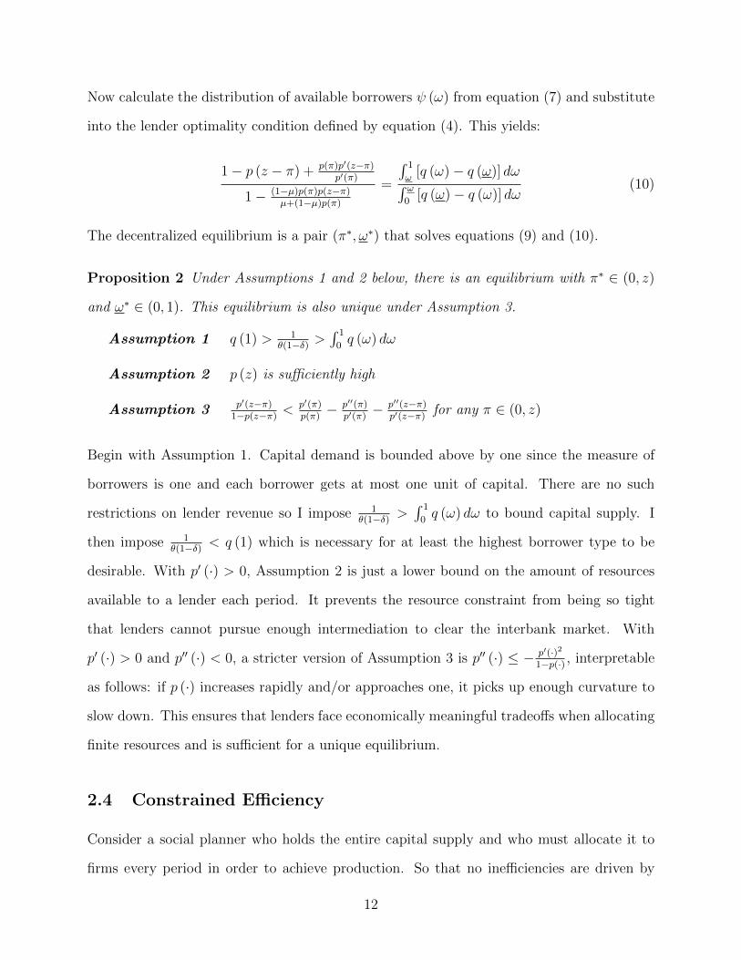
The decentralized equilibrium is a pair (π∗, ω∗) that solves equations (9) and (10).

Proposition 2 Under Assumptions 1 and 2 below, there is an equilibrium with π∗ ∈ (0, z)

and ω∗ ∈ (0, 1). This equilibrium is also unique under Assumption 3.

Assumption 1 q (1) > 1θ(1−δ) >

∫ 1

0q (ω) dω

Assumption 2 p (z) is sufficiently high

Assumption 3 p′(z−π)1−p(z−π)

< p′(π)p(π)− p′′(π)

p′(π)− p′′(z−π)

p′(z−π)for any π ∈ (0, z)

Begin with Assumption 1. Capital demand is bounded above by one since the measure of

borrowers is one and each borrower gets at most one unit of capital. There are no such

restrictions on lender revenue so I impose 1θ(1−δ) >

∫ 1

0q (ω) dω to bound capital supply. I

then impose 1θ(1−δ) < q (1) which is necessary for at least the highest borrower type to be

desirable. With p′ (·) > 0, Assumption 2 is just a lower bound on the amount of resources

available to a lender each period. It prevents the resource constraint from being so tight

that lenders cannot pursue enough intermediation to clear the interbank market. With

p′ (·) > 0 and p′′ (·) < 0, a stricter version of Assumption 3 is p′′ (·) ≤ − p′(·)21−p(·) , interpretable

as follows: if p (·) increases rapidly and/or approaches one, it picks up enough curvature to

slow down. This ensures that lenders face economically meaningful tradeoffs when allocating

finite resources and is sufficient for a unique equilibrium.

2.4 Constrained Efficiency

Consider a social planner who holds the entire capital supply and who must allocate it to

firms every period in order to achieve production. So that no inefficiencies are driven by

12

differences in assumptions, the planner faces the same technologies and constraints as lenders

in the decentralized economy. In particular, the fraction of available firms reached by the

planner is p (π) and, out of these firms, he is informed about fraction p (z − π). The worst

firm he allocates to when informed is ω. The planner chooses π ∈ [0, z] and ω ∈ [0, 1] to

maximize the total present discounted value of output, W ≡ µθ1−β

∫ 1

0q (ω) [λ (ω) + φ (ω)] dω,

subject to equations (5), (6), and (8). In this context, equation (8) is the planner’s aggregate

feasibility constraint. Combining the planner’s first order conditions for π and ω yields:

1− p (z − π) + p(π)p′(z−π)p′(π)(

1− (1−µ)p(π)p(z−π)µ+(1−µ)p(π)

)2 =

∫ 1

ω[q (ω)− q (ω)] dω∫ ω

0[q (ω)− q (ω)] dω

(11)

The constrained efficient allocation is a pair (π, ω) that solves equations (9) and (11).

Proposition 3 If µ is not too close to zero and q′′ (·) is not too low, (π, ω) is unique.

The above proposition restricts q (·) to being convex, linear, or mildly concave. In other

words, some differences in borrower quality should also be visible among higher types.

2.5 Main Results

The following proposition summarizes the first main result of this paper:

Proposition 4 Invoke Assumptions 1, 2, and the conditions in Proposition 3. Any equilib-

rium is constrained efficient if and only if µ = 1. The direction of inefficiency for µ < 1 is

π∗ > π with ω∗ > ω, stated more compactly as (π∗, ω∗) (π, ω).

Both the planner and the decentralized solution have equation (9) in common so any

inefficiencies reflect differences in equations (10) and (11). There are no differences in these

equations if µ = 1, making the equilibrium constrained efficient. Notice that µ = 1 results

in all matches being destroyed at the end of the period. In other words, the pool from which

unmatched lenders draw matches is always the initial pool. The equilibrium only being

13

efficient in this case suggests that the externalities associated with µ < 1 arise because of

intertemporal match preservation. In particular, a lender who engages in both matching and

screening will have a positive probability of forming an informed match. If the borrower is

desirable (i.e., if ω ≥ ω), then the match is retained and unavailable to other lenders until it

matures. If the borrower is undesirable (i.e., if ω < ω), then the match is rejected and the

borrower returns to the available pool. Resource allocation thus determines the probability

with which a lender worsens the pool of borrowers available to other lenders. Note that the

externality is on the quality of this pool: matching is one-to-one and the number of available

borrowers always equals the number of available lenders so it is the likelihood of getting a

desirable borrower that worsens, not the likelihood of getting any borrower at all.

The distributional externality just described involves both matching and screening yet

π∗ > π as per Proposition 4 suggests a negative externality associated primarily with the

matching activity. The distributional intuition must therefore be made more precise. As a

first step, it will be instructive to compare my model with other banking models that also

feature distributional externalities (i.e., winner’s curse models). In Direr (2008), for example,

high screening by all lenders worsens the available pool so each individual lender does indeed

have an incentive to incur screening costs. Low screening has the opposite effect, resulting in

both “low screening” and “high screening” equilibria. While high screening in my model also

increases the fraction of matched borrowers that are discovered, the diversion of resources

from matching to screening means there are very few matches to being with. The number

of matched borrowers who are discovered is therefore quite low, reducing the effect on the

available borrower pool. Modeling the cost of screening as foregone matching rather than a

reduced-form screening cost thus circumvents a “high screening” equilibrium.

Modeling an interbank clearing cost r and an endogenous threshold ω – two other dimen-

sions along which my model and standard winner’s curse models differ – also has important

implications. If ω were exogenous, then r could price the distributional externality and im-

plement constrained efficiency. Let me elaborate on this point. Exogenous ω eliminates equa-

14

tion (3) as an equilibrium condition and replaces∫ 1

0max J (ω)− (1 + r)− βU, 0ψ (ω) dω

in equation (2) with∫ 1

ω[J (ω)− (1 + r)− βU ]ψ (ω) dω for some constant ω. The equilibrium

would then be a triple U, π, r which solves the new version of (2), the resulting first order

condition for π, and interbank clearing as per equation (9). Equation (9) is common to both

the planner and the market so a given ω pins down π∗ and π at the same point, with r

adjusting to deliver this point from the remaining equilibrium conditions. The adjustment

mechanism can be understood as follows: π∗ > π implies that too many low quality borrow-

ers are being financed so the resulting destruction of interbank capital bids up the cost of

funds r, decreasing the benefit of an average match and thus decreasing π∗.

We can now conclude that inefficiency under µ < 1 involves a distributional externality as

well as an inability of r to properly price this externality when ω is endogenous. Endogeneity

of ω means that the lowest type retained by an informed lender is the type that gives him his

outside option. This option is the present discounted value of being unmatched so ω∗ > ω as

in Proposition 4 suggests that βU is too large. Resource allocation affects βU in two ways.

First, it changes the distribution of borrowers from which unmatched lenders draw. Second,

for any given distribution, the allocation is chosen to maximize the value of being unmatched.

Therefore, even with an adversely selected distribution, the matching probability may be high

enough to reduce the expected duration until a good draw and convince informed lenders to

break more matches. Indeed, in the present environment, a high matching probability means

that not a lot of screening is taking place so the distributional externality may actually be

quite small. Notice the role of the matching versus screening tradeoff here: if screening

were costless, then high π would be associated with a dramatic reduction in the quality of

available borrowers so, even with a high matching probability, informed lenders may not

want to be very selective.

Putting everything together, the negative externality associated with matching has two

parts. The first part is a distributional externality which emerges most strongly when π is

increased from an initially low value. Increasing π in this case helps match formation more

15

than it hurts type discovery. The resulting boost in informed matching negatively affects

the distribution of available borrowers. The second part is an outside option externality

which emerges most strongly when π is increased from an initially high value. Increasing π

here hurts type discovery more than it helps match formation. Although this weakens the

distributional deterioration, a weaker deterioration combined with a higher matching rate

increases the relative value of being unmatched and negatively affects informed retention.

Internalizing the effects of resource allocation on both the unmatched and informed prob-

lems leads the planner to prescribe (π, ω) (π∗, ω∗). In words, the planner devotes more

resources to screening new matches but is less restrictive in his cutoff once informed. Effec-

tively then, unmatched lenders are too liberal while informed lenders are too conservative. It

is this tension that confounds the ability of r to implement (π, ω) as an equilibrium: π∗ too

high increases r by destroying interbank capital but ω∗ too high decreases r by decreasing

the demand for such capital so the adjustment mechanism is stunted in either direction.10

The next proposition summarizes the aggregate implications of Proposition 4:

Proposition 5 If µ < 1, then: (i) uninformed lending is too high; (ii) informed lending is

too low; (iii) total lending is too low; (iv) the average default rate is constrained efficient.

The first two parts of Proposition 5 are intuitive given that unmatched lenders overdo match-

ing relative to screening while informed lenders are too selective in the types they retain.

The third part then reveals that the composition of informed versus uninformed lending

results in an inefficiently small credit market overall. Both screening and total credit being

inefficiently low contrasts with Dell’Ariccia and Marquez (2006). Moreover, the fact that my

model can deliver these features without assuming bad economic prospects contrasts with

Ruckes (2004). The joint determination of matching, screening, and retention thus provides

new insight into the relationship between lending standards and lending volumes.

10Prior to this, we saw two cases where the adjustment mechanism worked: µ = 1 and ω fixed. With µ = 1,there is no distributional externality so the only externality imparted by resource allocation is maximizationof the unmatched value. However, just like r adjusts to price the distributional externality when ω is heldfixed, r adjusts to price in the direct effect on βU when the distributional externality is absent.

16

To understand the fourth part of Proposition 5, consider Figure 1 which shows the dis-

tribution of financed projects. On one hand, higher screening by the planner means that he

allocates a lower fraction of his capital to low quality projects. On the other hand though,

lower selectivity means that he ends up dividing the remaining fraction across a wider range

of project qualities. Relative to the market then, the planner allocates lower fractions of his

capital to both very good and very bad projects. Equation (9) is such that these differences

exactly offset, yielding a constant average default rate. I will return to this in Section 4.

For now, I just emphasize that the market has the same average default rate as the planner

but less capital to lend overall because the decentralized distribution of default rates is a

mean-preserving spread of the constrained efficient distribution.

2.6 Corrective Taxation

The results so far suggest a role for corrective taxation. As a benchmark, consider a scheme

which taxes lender revenues at a constant rate then remits the proceeds to the interbank

market. I refer to this scheme as a remitted revenue tax. Remittance ensures equation (9)

is unchanged but, from the perspective of an individual lender, the tax is isomorphic to an

increase in δ. Notice, however, that δ dropped out of equation (10). The two equations that

define (π∗, ω∗) are thus unchanged so the remitted revenue tax is entirely ineffective.

Consider now a scheme which taxes lending intensity π at a constant rate τ then remits

the proceeds to the interbank market. I refer to this scheme as a remitted matching tax.

Remittance again ensures that equation (9) is unchanged but, from the perspective of an

individual lender, the tax subtracts τπ from the maximization problem in equation (2). As

shown next, the matching tax succeeds where the revenue tax failed:

Proposition 6 There is a τ > 0 that implements (π, ω) as an equilibrium.

The comparison between revenue and matching taxes reiterates the nature of the inefficiencies

discussed in Subsection 2.5. In particular, addressing the underlying externalities requires

17

targeting the resource allocation decision: a more general tax is not enough.11

3 Extension: Relationship Lending

By dissolving matches after one project, Section 2 shut out relationship lending – that is, the

acquisition of information about a particular borrower over repeated interactions and the use

of that information in subsequent financing. An ability to resolve information frictions over

time could have important implications for the allocation of resources between matching and

screening so it is natural to ask how relationship lending affects the baseline results.

A simple way to incorporate relationship lending is to distinguish between the time to

project completion and the time to exogenous match separation. In the baseline model,

these two events coincided and were geometrically distributed with parameter µ ∈ (0, 1]. I

now model only the time to exogenous separation as being geometrically distributed: the

time to project completion will instead be fixed at one period. A lender who is still matched

at the end of date t thus decides whether to finance another project for his borrower at the

beginning of date t+ 1 (i.e., whether to retain the borrower again). If the date t match was

informed, then the lender enters date t+1 still informed. If the date t match was uninformed,

then the lender becomes informed at the beginning of date t+ 1 by virtue of having engaged

with the borrower during date t. To ensure that the number of available borrowers still

equals the number of available lenders without any further changes to the baseline model,

assume learning via relationship lending occurs after the matching stage. Also assume no

intertemporal commitment to keep the contracting space in line with the baseline model.

Optimization Problems I will use tildes to distinguish the endogenous objects in the

relationship lending model from their baseline counterparts. Since informed lenders can now

11In practice, τ could be interpreted as either a direct tax on the number of loans or a corporate governanceregulation enforced by bank examiners. Governance regulations are expounded by Kashyap et al (2008)insofar as they do not distort the “search for performance” that allows banks to allocate resources. As Ishow, however, the decentralized allocation of internal bank resources is itself distorted so there is additionalscope for bank examiners to monitor the composition of a bank’s workforce and levy costs accordingly.

18

make multiple retention decisions over the course of one match, I will also define an explicit

value function for them. In particular, let JI (ω) denote the value of an informed lender

who is matched with a type ω borrower. If the lender rejects, then he gets zero in the

current period and begins next period unmatched. If the lender accepts (i.e., retains), then

his expected payoff in the current period is θ (1− δ) q (ω) − (1 + r) and he faces the same

accept/reject choice next period provided the match is not exogenously destroyed. Therefore:

JI (ω) = max[θ (1− δ) q (ω)− (1 + r) + β (1− µ) JI (ω) + βµU

], βU

(12)

The value of an unmatched lender, U , is now given by the following Bellman equation:

U = maxπ∈[0,z]

p (π) [p (z − π) + β (1− µ) [1− p (z − π)]]

∫ 1

0JI (ω) ψ (ω) dω

+p (π) [1− p (z − π)]∫ 1

0

[θ (1− δ) q (ω)− (1 + r) + βµU

]ψ (ω) dω

+ [1− p (π)] βU

(13)

Retention decisions can again be shown to follow a reservation strategy. In particular, an

informed lender will only retain ω ∈ [ω, 1], where JI (ω) ≡ βU . I defer the proof until

Proposition 7. What I want to highlight instead is the key difference between equation (13)

and the unmatched problem in the baseline model: the weight assigned to becoming an

informed lender. An unmatched lender clearly becomes informed when both his matching

and screening activities succeed. This is as before and occurs with probability p (π) p (z − π).

Now, however, the lender also has a way of becoming informed when only his matching

activity succeeds. This occurs with probability p (π) [1− p (z − π)] but is discounted by

β (1− µ) since relationship lending informs him next period provided the match survives.

The discount factor β will thus affect an unmatched lender’s assessment of how well learning

through relationship lending substitutes for screening.

Aggregate Conditions The distribution of available borrowers and the interbank clearing

condition are still given by equations (7) and (8) but with the following laws of motion for

19

uninformed and informed matches respectively:

φ (ω) =[1− (1− µ)

[λ (ω) + φ (ω)

]]p (π) [1− p (z − π)] (14)

µλ (ω) = I (ω ≥ ω)×[(1− µ) φ (ω) +

[1− (1− µ)

[λ (ω) + φ (ω)

]]p (π) p (z − π)

](15)

The difference between these equations and their baseline counterparts is the flow from

uninformed to informed matches. With relationship lending, any uninformed matches not

lost to exogenous separation become informed. Comparing to equations (5) and (6), we thus

have an extra outflow (1− µ) φ (ω) in (14) and an extra inflow (1− µ) φ (ω) in (15). Notice

that the extra inflow in (15) is subject to the retention decision I (ω ≥ ω). Therefore, for

the same values of π and ω, the relationship lending model will have a worse distribution of

available borrowers than the baseline model.

Equilibrium The equilibrium can be synthesized as in Subsection 2.3. First, combine

interbank clearing with λ (·) and φ (·) to get the relationship lending version of equation (9):

1− p (z − π)

1 + (1−µ)[1−p(π)p(z−π)]µ+(1−µ)p(π)

=

∫ 1

ω

[q (ω)− 1

θ(1−δ)

]dω∫ ω

0

[1

θ(1−δ) − q (ω)]dω

(16)

Next, solve the optimization problem in equation (13). Combine the resulting first order

condition for π with JI (ω) ≡ βU and the Bellman equation for JI (·). Using λ (·) and φ (·)

to substitute out ψ (·) then yields the relationship lending version of equation (10):

1− p (z − π) + p(π)p′(z−π)p′(π)

µ(

1 + (1−µ)[1−p(π)p(z−π)]µ+(1−µ)p(π)

) =1

1− β (1− µ)

(∫ 1

ω[q (ω)− q (ω)] dω∫ ω

0[q (ω)− q (ω)] dω

)(17)

The decentralized equilibrium is a pair (π∗, ω∗) that solves equations (16) and (17). The

difference between (9) and (16) stems solely from distributional differences (i.e., λ (·) 6= λ (·)

and φ (·) 6= φ (·)) while the difference between (10) and (17) also involves the discount factor.

As we will see next, this introduces a special role for β.

20

Main Results The efficiency benchmark for the relationship lending model is similar to

Subsection 2.4. In particular, consider a social planner who chooses π ∈ [0, z] and ω ∈ [0, 1]

to maximize the total present discounted value of output subject to aggregate feasibility.12

Using λ (·) and φ (·) instead of λ (·) and φ (·), this maximization yields:

1− p (z − π) + p(π)p′(z−π)p′(π)

µ(

1 + (1−µ)[1−p(π)p(z−π)]µ+(1−µ)p(π)

)2 =

∫ 1

ω[q (ω)− q (ω)] dω∫ ω

0[q (ω)− q (ω)] dω

(18)

The constrained efficient allocation is a pair(˜π, ˜ω) that solves equations (16) and (18).

Neither equation depends on β so B in the following proposition is explicitly defined:

Proposition 7 The assumptions in Propositions 2 and 3 suffice for (π∗, ω∗) and(˜π, ˜ω) to

exist uniquely. Invoking these assumptions and defining B ≡ 1−p(˜π)p(z−˜π)1+(1−µ)p(˜π)[1−p(z−˜π)] ∈ (0, 1):

1. If µ = 1 or β = B, then the equilibrium is constrained efficient

2. If µ < 1 and β < B, then (π∗, ω∗)(˜π, ˜ω) but ∃ τ < 0 that implements

(˜π, ˜ω)3. If µ < 1 and β > B, then (π∗, ω∗)

(˜π, ˜ω) but ∃ τ > 0 that implements(˜π, ˜ω)

The key takeaway from Proposition 7 is existence of a discount factor that restores con-

strained efficiency. Recall that relationship lending changes the baseline model in two ways:

it provides an alternative to screening and it worsens the distribution of available borrowers.

Taken separately, a worse distribution gives unmatched lenders an incentive to choose lower

π while the ability to learn without screening gives them an incentive to choose higher π.

Equilibrium requires a fixed point where these two incentives exactly offset. By changing an

unmatched lender’s assessment of how well relationship lending substitutes for screening, β

changes where the exact offset occurs. There is one β for which it occurs at the constrained

efficient allocation. If β exceeds this critical value, then the inefficiency in Proposition 4 still

holds. It can then be verified that the macro implications in Proposition 5 also still hold.13

12Since successful projects now produce output in one period, the objective function in Subsection 2.4 istechnically scaled up by 1

µ . However, with µ constant, this has no bearing on the results.13The proof is similar to the proof of Proposition 5 and is thus omitted.

21

4 Extension: Moral Hazard

The analysis so far has abstracted from moral hazard: lenders were entitled to an exoge-

nous share of project output and borrowers behaved independently of this share. Rejecting

borrowers with bad projects was thus the only motive to screen. A moral hazard problem

on the borrower side may introduce additional screening motives (i.e., extracting more from

borrowers with good projects). Do the core results of Propositions 4 and 5 change in any

meaningful way? As I show below, the only qualitative difference with moral hazard is the

potential for constrained inefficiency of the average default rate. On the quantitative side,

there are additional insights about the size of the welfare loss.

4.1 Borrower Problem

Return to the environment of Section 2. A successful project still yields θ upon completion

but the success probability now depends on how much effort the borrower exerts when the

completion period arrives. In particular, a type ω who exerts effort e ∈ [0, 1] succeeds with

probability eα (ω), where α (·) ∈ [0, 1], α′ (·) > 0, and α′′ (·) ≤ 0. Success allows ω to

consume θ − R, where R is the gross loan rate charged by the lender. However, exerting e

imparts a disutility of −c ln (1− e) on the borrower, where c > 0 is a constant.14 Matches

are dissolved upon project completion so each match is defined by one R. The borrower thus

chooses e ∈ [0, 1] to maximize eα (ω) [θ −R]+c ln (1− e), resulting in the following strategy:

e (ω,R) =

1− cα(ω)[θ−R]

if R < θ − cα(ω)

0 if R ≥ θ − cα(ω)

(19)

There are two differences relative to Section 2. First, success probabilities are given by

e (ω,R)α (ω) rather than q (ω). Second, the lender share of project output is R/θ rather

than 1 − δ. The rest of the baseline environment stands so the additional insights of the

moral hazard model will come entirely from making R an equilibrium object.

14This functional form rules out the corner choice of e = 1 and thus conserves on algebra.

22

4.2 Loan Rate Choice

Consider a lender who finances type ω at loan rate R. The lender’s expected payoff in the

completion period is now e (ω,R)α (ω)R instead of θ (1− δ) q (ω). If informed, the lender

can condition his loan rate choice on ω. Otherwise, he can only offer a pooled rate that

conditions on the distribution ψ (·). This has two implications. First, the lender’s loan

rate will depend on the success of his screening activity. Second, informed and uninformed

matches are no longer identical for desirable types so loan rates must be chosen subject to a

borrower participation constraint. For analytical tractability, I focus on equilibria where such

constraints do not bind (i.e., equilibria where the unconstrained loan rates satisfy borrower

participation). Loan rate offers are take-it-or-leave-it but equation (19) imposes an important

restriction: higher rates induce lower repayment probabilities so lenders must share surplus.

Proposition 8 Suppose c ≤ θα(0)2

α(1). Any symmetric steady state with non-binding borrower

participation constraints takes the form (π, ω). Informed lenders charge R (ω) = θ −√

cθα(ω)

and uninformed lenders charge R (π, ω) = θ−√

cθα(π,ω)

, where α (π, ω) ≡∫ 10 α(ω)dω+σ(π)

∫ ω0 α(ω)dω

1+σ(π)ω

and σ (π) ≡ (1−µ)p(π)p(z−π)µ+(1−µ)p(π)[1−p(z−π)]

. Moreover, all financed borrowers exert positive effort.

To make the notation more compact, combine Proposition 8 with the expected payoff

e (ω,R)α (ω)R. In particular, define:

g (ω) ≡ e (ω,R (ω))α (ω)R (ω) =(√

θα (ω)−√c)2

h(ω,R (·)

)≡ e

(ω,R (·)

)α (ω)R (·) =

(α (ω)− c

θ−R(·)

)R (·)

Also define the difference D(ω,R (·)

)≡ g (ω)− h

(ω,R (·)

). An informed lender can always

charge R (·) instead of R (ω) so D(ω,R (·)

)≥ 0 with strict inequality for at least some ω.

4.3 Incorporating into Baseline Environment

We can now derive the moral hazard versions of equations (9) and (10) that would prevail

under Proposition 8. Begin with equation (9) which captured equilibrium in the interbank

23

market. The capital needed to finance new loans is still µ∫ 1

0[λ (ω) + φ (ω)] dω but the

capital available from maturing loans is now µ[∫ 1

0g (ω)λ (ω) dω +

∫ 1

0h(ω,R (·)

)φ (ω) dω

]so the moral hazard version of equation (9) becomes:

1− p (z − π)

1− (1−µ)p(π)p(z−π)µ+(1−µ)p(π)

=

∫ 1

ω[g (ω)− 1] dω∫ ω

0[1− g (ω)] dω + ∆ (π, ω)

(20)

where

∆ (π, ω) ≡∫ ω

0D(ω,R (π, ω)

)dω +

(1− (1−µ)p(π)p(z−π)

µ+(1−µ)p(π)

) ∫ 1

ωD(ω,R (π, ω)

)dω

Turn now to equation (10) which captured optimality of π. Using the expected payoffs under

moral hazard, the lender value functions become:

U = maxπ∈[0,z]

p (π) p (z − π)∫ 1

0max JI (ω)− (1 + r)− βU, 0ψ (ω) dω

+p (π) [1− p (z − π)]∫ 1

0[JN (ω)− (1 + r)− βU ]ψ (ω) dω + βU

where

JI (ω) = µ [g (ω) + βU ] + (1− µ) βJI (ω)

JN (ω) = µ[h(ω,R (·)

)+ βU

]+ (1− µ) βJN (ω)

The informed cutoff satisfies JI (ω) ≡ βU + (1 + r) and the computation of ψ (·) proceeds

as before so the moral hazard version of equation (10) amounts to:

1− p (z − π) + p(π)p′(z−π)p′(π)

1− (1−µ)p(π)p(z−π)µ+(1−µ)p(π)

=

∫ 1

ω[g (ω)− g (ω)] dω∫ ω

0[g (ω)− g (ω)] dω + ∆ (π, ω)

(21)

The decentralized equilibrium is now a pair (π∗, ω∗) that solves equations (20) and (21) and

is internally consistent with Proposition 8. Notice that imposing g (·) = h (·) = θ (1− δ) q (·)

on equations (20) and (21) recovers their baseline counterparts.

Proposition 9 Define a ≡ α (1)−√

α(1)θ

and assume the following:

24

Assumption 4 p′(z−π)1−p(z−π)

∈[−1

2

(p′′(π)p′(π)

+ p′′(z−π)p′(z−π)

),−(p′′(π)p′(π)

+ p′′(z−π)p′(z−π)

)]for any π ∈ (0, z)

There exist scalars a ∈ (0, a), p ∈ (0, 1), p ∈ (0, p), c ∈(

0, θα(0)2

α(1)

), and c ∈ [0, c) such that

α (0) ∈ (a, a), p (z) ∈[p, p], and c ∈ [c, c] are sufficient for a unique symmetric steady state

with non-binding borrower participation constraints.

Assumption 4 imposes somewhat stricter conditions on the curvature of p (·) than Assump-

tion 3. The parameter bounds are also somewhat stricter than simple analogs of the remain-

ing baseline assumptions. These additional restrictions help make tractable the complexity

that stems from interactions between π, ω, and R (·) under moral hazard.

4.4 Comparison to Baseline Results

To proceed, we need an efficiency benchmark for the moral hazard model. Along with

choosing π ∈ [0, z] and ω ∈ [0, 1], the planner must now divide output between consumption

and capital. In particular, if he allocates one unit of capital to firm ω when informed and

ω succeeds in producing θ, then κ (ω) is returned to the planner as capital and θ − κ (ω) is

consumed by the firm. A similar statement applies when the planner is uninformed but with κ

in place of κ (ω). I begin by considering a planner that maximizes the total present discounted

value of capital subject to aggregate feasibility. A more conventional welfare measure is taken

up in Subsection 4.5 but capital maximization provides a useful starting point. To see why,

recall that lenders are the only source of saving in the decentralized economy so loan rates

ultimately dictate the decentralized division of output between consumption and capital (i.e.,

R (ω) and R play the same role as κ (ω) and κ). Since lenders choose this division to maximize

capital, they will automatically be inefficient if judged against a planner who maximizes net

output. Notice that this inefficiency stems from borrowers not being able to store and arises

even if π and ω are treated as model parameters. Considering a capital-maximizing planner

is one way to generate a constrained efficiency benchmark that is also constrained by the

storage assumption. The derivation appears in the appendix and it produces the following

25

moral hazard version of equation (11):

1− p (z − π) + p(π)p′(z−π)p′(π)(

1− (1−µ)p(π)p(z−π)µ+(1−µ)p(π)

)2 =

∫ 1

ω[g (ω)− g (ω)] dω − (1−µ)p(π)[1−p(z−π)]

µQ (π, ω)∫ ω

0[g (ω)− g (ω)] dω + ∆ (π, ω)

(22)

where

∆ (π, ω) ≡∫ ω

0D(ω,R (π, ω)

)dω +

(1− (1−µ)p(π)p(z−π)

µ+(1−µ)p(π)

)2 ∫ 1

ωD(ω,R (π, ω)

)dω

Q (π, ω) ≡(

1− ω +1−p(z−π)+

p(π)p′(z−π)p′(π)

(1− (1−µ)p(π)p(z−π)µ+(1−µ)p(π) )

2 ω

)D(ω,R (π, ω)

)+ p(π)p′(z−π)

p′(π)[1−p(z−π)]

∫ 1

ωD(ω,R (π, ω)

)dω

The constrained efficient allocation is a pair (π, ω) that solves equations (20) and (22). Im-

posing g (·) = h (·) = θ (1− δ) q (·) on equation (22) again recovers the baseline counterpart.

Proposition 10 For µ < 1, the steady state of Proposition 9 is such that (π∗, ω∗) (π, ω)

but there exists a τ > 0 that implements (π, ω).

Proposition 10 confirms the core inefficiency result in Proposition 4. Since the laws of motion

for λ (·) and φ (·) are also unchanged from the baseline model, it is trivial to show that the

first three parts of Proposition 5 continue to hold. In particular, the moral hazard model still

predicts too much uninformed credit, too little informed credit, and too little total credit.

The default prediction, however, is now ambiguous. A maturing project financed at loan

rate R defaults with probability 1− e (ω,R)α (ω) so the economy’s average default rate is:

µ

[1−

∫ 1

0

e (ω,R (ω))α (ω) λ(ω)∫ 10 [λ(x)+φ(x)]dx

dω −∫ 1

0

e(ω,R (·)

)α (ω) φ(ω)∫ 1

0 [λ(x)+φ(x)]dxdω

]

This can be rewritten as µ

[1−

∫ 10 e(ω,R(ω))α(ω)λ(ω)dω+

∫ 10 e(ω,R(·))α(ω)φ(ω)dω∫ 1

0 e(x,R(x))α(x)R(x)λ(x)dω+∫ 10 e(x,R(·))α(x)R(·)φ(x)dx

]since interbank

clearing equates µ∫ 1

0[λ (x) + φ (x)] dx to the capital available from maturing loans. In the

baseline model, R (ω) = R (·) = θ (1− δ) so interbank clearing was enough to make the

average default rate a constant. This is no longer the case in the model hazard model.

Therefore, the inefficiency result of Proposition 10 will also be transmitted to defaults.

26

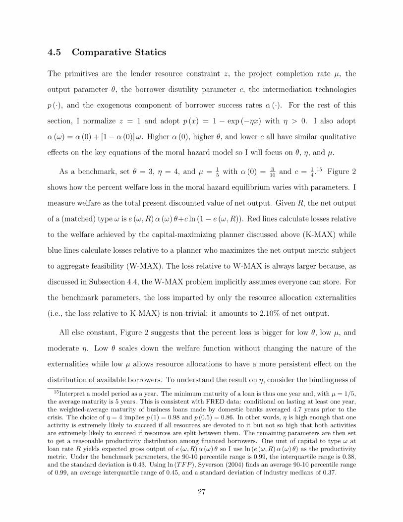
4.5 Comparative Statics

The primitives are the lender resource constraint z, the project completion rate µ, the

output parameter θ, the borrower disutility parameter c, the intermediation technologies

p (·), and the exogenous component of borrower success rates α (·). For the rest of this

section, I normalize z = 1 and adopt p (x) = 1 − exp (−ηx) with η > 0. I also adopt

α (ω) = α (0) + [1− α (0)]ω. Higher α (0), higher θ, and lower c all have similar qualitative

effects on the key equations of the moral hazard model so I will focus on θ, η, and µ.

As a benchmark, set θ = 3, η = 4, and µ = 15

with α (0) = 310

and c = 14.15 Figure 2

shows how the percent welfare loss in the moral hazard equilibrium varies with parameters. I

measure welfare as the total present discounted value of net output. Given R, the net output

of a (matched) type ω is e (ω,R)α (ω) θ+c ln (1− e (ω,R)). Red lines calculate losses relative

to the welfare achieved by the capital-maximizing planner discussed above (K-MAX) while

blue lines calculate losses relative to a planner who maximizes the net output metric subject

to aggregate feasibility (W-MAX). The loss relative to W-MAX is always larger because, as

discussed in Subsection 4.4, the W-MAX problem implicitly assumes everyone can store. For

the benchmark parameters, the loss imparted by only the resource allocation externalities

(i.e., the loss relative to K-MAX) is non-trivial: it amounts to 2.10% of net output.

All else constant, Figure 2 suggests that the percent loss is bigger for low θ, low µ, and

moderate η. Low θ scales down the welfare function without changing the nature of the

externalities while low µ allows resource allocations to have a more persistent effect on the

distribution of available borrowers. To understand the result on η, consider the bindingness of

15Interpret a model period as a year. The minimum maturity of a loan is thus one year and, with µ = 1/5,the average maturity is 5 years. This is consistent with FRED data: conditional on lasting at least one year,the weighted-average maturity of business loans made by domestic banks averaged 4.7 years prior to thecrisis. The choice of η = 4 implies p (1) = 0.98 and p (0.5) = 0.86. In other words, η is high enough that oneactivity is extremely likely to succeed if all resources are devoted to it but not so high that both activitiesare extremely likely to succeed if resources are split between them. The remaining parameters are then setto get a reasonable productivity distribution among financed borrowers. One unit of capital to type ω atloan rate R yields expected gross output of e (ω,R)α (ω) θ so I use ln (e (ω,R)α (ω) θ) as the productivitymetric. Under the benchmark parameters, the 90-10 percentile range is 0.99, the interquartile range is 0.38,and the standard deviation is 0.43. Using ln (TFP ), Syverson (2004) finds an average 90-10 percentile rangeof 0.99, an average interquartile range of 0.45, and a standard deviation of industry medians of 0.37.

27

the lender resource constraint. Low η (relative to z) implies a tight constraint: an unmatched

lender does not have enough resources to make even one intermediation activity succeed

with high probability. The fraction of matches that are informed is thus small, making

the distributional externality small as well. The inability to rematch at a high rate then

helps disincentivize informed lenders from breaking more matches in response to the smaller

distributional deterioration. Low values of η thus dampen the externalities discussed in

Subsection 2.5 and result in a smaller welfare loss. Increasing η relaxes the bindingness of

the resource constraint and initially increases the welfare loss. However, as η continues to

increase, it becomes possible to make both matching and screening succeed with probabilities

very close to one. In other words, the constraint all but disappears, resource allocation

becomes moot, and the welfare loss relative to K-MAX tends to zero.

Figure 2 also plots the welfare losses predicted by the baseline model when q (ω) = g(ω)θ(1−δ) .

Recall that the moral hazard model distinguishes between an expected payoff of g (ω) for

informed lenders and an expected payoff of h(ω,R (π, ω)

)for uninformed lenders. Under the

posited q (ω), the baseline model uses g (ω) for both. Figure 2 shows that the welfare loss is

almost always smaller in the baseline: not having the externalities feed through uninformed

loan rates attenuates the loss.

As a final exercise, Figure 3 explores whether using W-MAX rather than K-MAX as

the efficiency benchmark for the moral hazard model changes any of the qualitative results.

Proposition 10 established (π∗, ω∗) (π, ω) when (π, ω) is chosen by a capital-maximizing

planner. The first column of Figure 3 reveals that the same result prevails under a welfare-

maximizing planner provided µ and η are not too high. The externalities imparted by

individual resource allocation decisions die out as µ and η get very large, leaving only the

failure of lenders to internalize their monopoly on storage. We can thus interpret Figure 3 as

saying that W-MAX also predicts (π∗, ω∗) (π, ω) for parameters where the externalities

I am concerned with are strongest. Turn next to the size of the overall credit market.

As discussed in Subsection 4.4, the decentralized market is too small relative to K-MAX.

28

Since a welfare-maximizing planner cares about both capital and consumption, he should

also settle on less capital than the capital-maximizing planner. However, for parameters

where my externalities are sufficiently strong, the second column of Figure 3 reveals that

the decentralized market is too small even when judged against W-MAX. The third column

then shows that the W-MAX comparison yields an unambiguous prediction about the average

default rate: it is always too high in the decentralized market. Relative to K-MAX though,

the decentralized rate could be either too high or too low. The orders of magnitude are small

but it is generally too high for parameters where the externalities I am concerned with are

strongest.

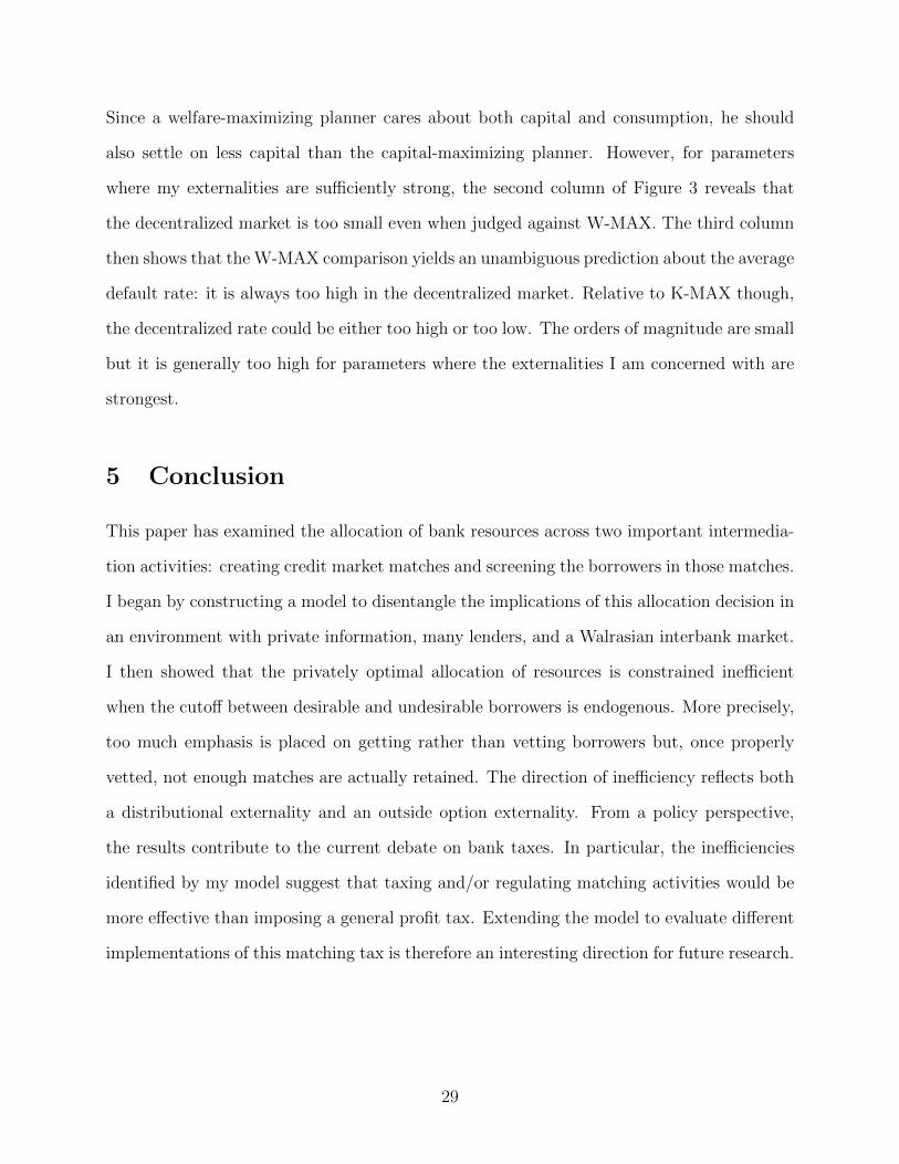
5 Conclusion

This paper has examined the allocation of bank resources across two important intermedia-

tion activities: creating credit market matches and screening the borrowers in those matches.

I began by constructing a model to disentangle the implications of this allocation decision in

an environment with private information, many lenders, and a Walrasian interbank market.

I then showed that the privately optimal allocation of resources is constrained inefficient

when the cutoff between desirable and undesirable borrowers is endogenous. More precisely,

too much emphasis is placed on getting rather than vetting borrowers but, once properly

vetted, not enough matches are actually retained. The direction of inefficiency reflects both

a distributional externality and an outside option externality. From a policy perspective,

the results contribute to the current debate on bank taxes. In particular, the inefficiencies

identified by my model suggest that taxing and/or regulating matching activities would be

more effective than imposing a general profit tax. Extending the model to evaluate different

implementations of this matching tax is therefore an interesting direction for future research.

29

References

Allen, F. and D. Gale. 2005. “From Cash-in-the-Market Pricing to Financial Fragility.”Journal of the European Economic Association, 3(2-3): 535-546.

Becsi, Z., V. Li, and P. Wang. 2013. “Credit Mismatch and Breakdown.” European EconomicReview, 59(1): 109-125.

Bernanke, B. and M. Gertler. 1989. “Agency Costs, Net Worth and Business Fluctuations.”American Economic Review, 79(1): 14-31.

Boot, A. 2000. “Relationship Banking: What Do We Know?” Journal of Financial Interme-diation, 9(1): 7-25.

Broecker, T. 1990. “Credit-Worthiness Tests and Interbank Competition.” Econometrica,58(2): 429-452.

Cao, M. and S. Shi. 2001. “Screening, Bidding, and the Loan Market Tightness.” EuropeanFinance Review, 5(1-2): 21-61.

Dell’Ariccia, G. and R. Marquez. 2006. “Lending Booms and Lending Standards.” Journalof Finance, 61(5): 2511-2546.

Diamond, D. 1984. “Financial Intermediation and Delegated Monitoring.” Review of Eco-nomic Studies, 51(3): 393-414.

Direr, A. 2008. “Multiple Equilibria in Markets with Screening.” Journal of Money, Creditand Banking, 40(4): 791-798.

Freixas, X. and J. Rochet. 1997. Microeconomics of Banking. Cambridge: MIT Press.

Gehrig, T. and R. Stenbacka. 2011. “Decentralized Screening: Coordination Failure, MultipleEquilibria, and Cycles.” Journal of Financial Stability, 7(2): 60-69.

Gorton, G. and G. Pennacchi. 1995. “Banks and Loan Sales: Marketing Non-marketableAssets.” Journal of Monetary Economics, 35(3): 389-411.

Gromb, D. and D. Vayanos. 2002. “Equilibrium and Welfare in Markets with FinanciallyConstrained Arbitrageurs.” Journal of Financial Economics, 66(2-3): 361-407.

Gurley, J. and E. Shaw. 1955. “Financial Aspects of Economic Development.” AmericanEconomic Review, 45(4): 515-538.

Hachem, K. 2011. “Relationship Lending and the Transmission of Monetary Policy.” Journalof Monetary Economics, 58(6-8): 590-600.

Hauswald, R. and R. Marquez. 2006. “Competition and Strategic Information Acquisitionin Credit Markets.” Review of Financial Studies, 19(3): 967-1000.

30

Heider, F. and R. Inderst. 2012. “Loan Prospecting.” Review of Financial Studies, 25(8):2381-2415.

Hosios, A. 1990. “On the Efficiency of Matching and Related Models of Search and Unem-ployment.” Review of Economic Studies, 57(2): 279-298.

Kashyap, A., R. Rajan, and J. Stein. 2008. “Rethinking Capital Regulation.” In: Main-taining Stability in a Changing Financial System, Federal Reserve Bank of Kansas CitySymposium, 431-471.

Keys, B., T. Mukherjee, A. Seru, and V. Vig. 2010. “Did Securitization Lead to Lax Screen-ing? Evidence from Subprime Loans.” Quarterly Journal of Economics, 125 (1): 307-362.

Kiyotaki, N. and J. Moore. 1997. “Credit Cycles.” Journal of Political Economy, 105(2):211-248.

Korinek, A. 2011. “Systemic Risk-Taking: Amplification Effects, Externalities, and Regula-tory Responses.” European Central Bank Working Paper 1345.

Livshits, I., J. MacGee, and M. Tertilt. 2011. “Costly Contracts and Consumer Credit.”NBER Working Paper 17448.

Lorenzoni, G. 2008. “Inefficient Credit Booms.” Review of Economic Studies, 75(3): 809-833.

Parlour, C. and U. Rajan. 2001. “Competition in Loan Contracts.” American EconomicReview, 91(5): 1311-1328.

Purnanandam, A. 2011. “Originate-to-Distribute Model and the Subprime Mortgage Crisis.”Review of Financial Studies, 24(6): 1881-1915.

Rajan, R. 1994. “Why Bank Credit Policies Fluctuate: A Theory and Some Evidence.”Quarterly Journal of Economics, 109(2): 399-441.

Ruckes, M. 2004. “Bank Competition and Credit Standards.” Review of Financial Studies,17(4): 1073-1102.

Shimer, R. and L. Smith. 2001. “Matching, Search, and Heterogeneity.” Advances in Macroe-conomics, 1(1): Article 5.

Shleifer, A. and R. Vishny. 2010. “Unstable Banking.” Journal of Financial Economics,97(3): 306–318.

Shleifer, A. and R. Vishny. 2011. “Fire Sales in Finance and Macroeconomics.” Journal ofEconomic Perspectives, 25(1): 29-48.

Stein, J. 1998. “An Adverse-Selection Model of Bank Asset and Liability Management withImplications for the Transmission of Monetary Policy.” RAND Journal of Economics,29(3): 466-486.

31

Syverson, C. 2004. “Product Substitutability and Productivity Dispersion.” Review of Eco-nomics and Statistics, 86(2): 534–550.

Williamson, S. 1987. “Financial Intermediation, Business Failures, and Real Business Cy-cles.” Journal of Political Economy, 95(6): 1196-1216.

Yashiv, E. 2007. “Labor Search and Matching in Macroeconomics.” European EconomicReview, 51(8): 1859-1895.

32

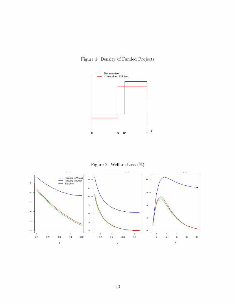
Figure 1: Density of Funded Projects

Density of Funded Projects

ωω10 ωω ωω*

DecentralizedConstrained Efficient

Figure 2: Welfare Loss (%)

2.8 2.9 3.0 3.1 3.2

01

23

45

Welfare Loss (%)

θθ

Relative to WMax Relative to KMaxBaseline

0.2 0.4 0.6 0.8

01

23

45

6

Welfare Loss (%)

µµ

2 4 6 8 10

01

23

4

Welfare Loss (%)

ηη

33

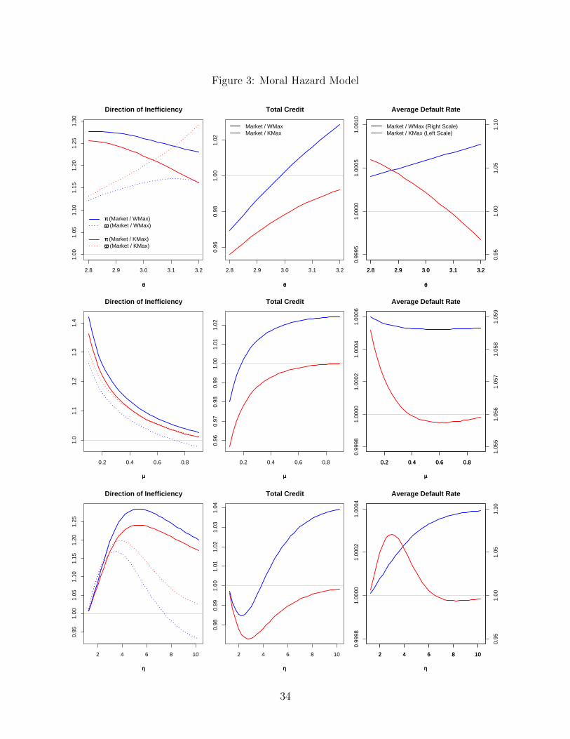
Figure 3: Moral Hazard Model

2.8 2.9 3.0 3.1 3.2

1.00

1.05

1.10

1.15

1.20

1.25

1.30

Direction of Inefficiency

θθ

ππ (Market / WMax)ωω (Market / WMax)

ππ (Market / KMax)ωω (Market / KMax)

2.8 2.9 3.0 3.1 3.2

0.96

0.98

1.00

1.02

Total Credit

θθ

Market / WMaxMarket / KMax

2.8 2.9 3.0 3.1 3.2

θθ

0.95

1.00

1.05

1.10

2.8 2.9 3.0 3.1 3.2

Average Default Rate

0.99

951.

0000

1.00

051.

0010

Market / WMax (Right Scale)Market / KMax (Left Scale)

0.2 0.4 0.6 0.8

1.0

1.1

1.2

1.3

1.4


µµ

0.2 0.4 0.6 0.8

0.96

0.97

0.98

0.99

1.00

1.01

1.02

Total Credit

µµ

0.2 0.4 0.6 0.8

µµ

1.05

51.

056

1.05

71.

058

1.05

9

0.2 0.4 0.6 0.8


0.99

981.

0000

1.00

021.

0004

1.00

06

2 4 6 8 10

0.95

1.00

1.05

1.10

1.15

1.20

1.25


ηη

2 4 6 8 10

0.98

0.99

1.00

1.01

1.02

1.03

1.04

Total Credit

ηη

2 4 6 8 10

ηη

0.95

1.00

1.05

1.10

2 4 6 8 10


0.99

981.

0000

1.00

021.

0004

34

Appendix - Proofs

Proof of Proposition 1

Define S ≡ r, ψ and write U (S) to make explicit that S is taken as given. Objects of

the form max x1, x2 can be expressed as maxa∈[0,1]

ax1 + (1− a)x2 so equations (1) and (2)

define the following mapping:

T U (S) = maxπ∈[0,z], a(·)∈[0,1]

` (π, a (·) , S) + y (π, a (·) , S) βU (S)

where

` (π, a (·) , S) ≡∫ 1

0p (π) [1− [1− a (ω)] p (z − π)]

[µθ(1−δ)q(ω)1−β(1−µ)

− (1 + r)]ψ (ω) dω

y (π, a (·) , S) ≡ 1− p (π)[1−

[1−

∫ 1

0a (ω)ψ (ω) dω

]p (z − π)

](1−β)(1−µ)1−β(1−µ)

If U exists in the set of bounded and continuous functions (C), then the Theorem of the

Maximum implies T U (S) ∈ C. Therefore, T : C → C. The following shows that T satisfies

Blackwell’s sufficient conditions for a contraction:

• (discounting) Consider U1 ∈ C and a constant k > 0:

T (U1 + k) = maxπ∈[0,z], a(·)∈[0,1]

` (π, a (·) , S) + y (π, a (·) , S) β (U1 + k)

= maxπ∈[0,z], a(·)∈[0,1]

` (π, a (·) , S) + y (π, a (·) , S) βU1 + y (π, a (·) , S) βk

≤ maxπ∈[0,z], a(·)∈[0,1]

` (π, a (·) , S) + y (π, a (·) , S) βU1+ βk = T U1 + βk

The inequality stems from y (π, a (·) , S) ∈ (0, 1] for all π ∈ [0, z] and a (·) ∈ [0, 1].

• (monotonicity) Consider U1, U2 ∈ C where U1 (·) ≥ U2 (·) and let π∗i , a∗i (·) denote

the optimal choices under Ui:

T U1 (S) = ` (π∗1, a∗1 (·) , S) + y (π∗1, a

∗1 (·) , S) βU1 (S)

≥ ` (π∗2, a∗2 (·) , S) + y (π∗2, a

∗2 (·) , S) βU1 (S)

≥ ` (π∗2, a∗2 (·) , S) + y (π∗2, a

∗2 (·) , S) βU2 (S) = T U2 (S)

The first inequality follows from the fact that π∗2, a∗2 (·) is feasible under U1. The

second inequality follows from y (π, a (·) , S) > 0 for all π ∈ [0, z] and a (·) ∈ [0, 1] along

with the assumption that U1 (·) ≥ U2 (·).

We can now invoke the Contraction Mapping Theorem to establish existence of a unique

U ∈ C such that U = T U .

35


Let πk (ω) and πl (ω) denote the functions implicitly defined by equations (9) and (10) re-

spectively. Proving existence of equilibrium thus requires proving existence of a pair (π∗, ω∗)

such that π∗ = πl (ω∗) = πk (ω∗).

Begin with equation (9). Define ξ such that q (ξ) ≡ 1θ(1−δ) . Assumption 1 and q′ (·) > 0

imply q (1) > 1θ(1−δ) > q (0) so ξ exists uniquely and is interior. Differentiating (9) reveals

π′k (ξ) = 0 and π′k (ω) [q (ω)− q (ξ)] < 0 for ω 6= ξ. A necessary condition for π∗ > 0 is

πk (ξ) > 0. To ensure πk (ξ) > 0, we need p (z) >1

θ(1−δ)−∫ 10 q(ω)dω∫ ξ

0 [ 1θ(1−δ)−q(ω)]dω

which is the essence of

Assumption 2. We can now conclude existence of unique points ξk,1 ∈ (0, ξ) and ξk,2 ∈ (ξ, 1)

satisfying πk(ξk,1)≡ 0 and πk

(ξk,2)≡ 0. The restriction to ξk,1 > 0 and ξk,2 < 1 reflects

the fact that πk (·) is not defined at ω = 0 or ω = 1 under Assumption 1 and p (z) < 1.

Turn to equation (10). When evaluated at ω = ξ, the right-hand sides of (9) and (10)

are the same so Assumption 2 also ensures πl (ξ) > 0. We can then show πl (ξ) < πk (ξ) in

two steps. First, the left-hand side of (9) is increasing in π. Second, the left-hand side of

(10) equals the left-hand side of (9) plus a function of π. This function is zero if π = 0 and

positive otherwise. Therefore, πl (ξ) ≥ πk (ξ) is impossible. The following lemma completes

the existence proof by finding a point ω ∈[ξk,1, ξ

)such that πl (ω) > πk (ω):

Lemma 1 If πl(ξk,1)

exists, then πl(ξk,1)> πk

(ξk,1). If πl

(ξk,1)

does not exist, then there

is a point ωz ∈(ξk,1, ξ

)such that πl (ωz) = z > πk (ωz).

Proof. Equation (9) and the definition of ξk,1 yield:

1− p (z) =

∫ 1ξk,1

[q(ω)− 1θ(1−δ) ]dω∫ ξk,1

0 [ 1θ(1−δ)−q(ω)]dω

<

∫ 1ξk,1

[q(ω)−q(ξk,1)]dω∫ ξk,10 [q(ξk,1)−q(ω)]dω

where the inequality follows from q(ξk,1)< q (ξ) ≡ 1

θ(1−δ) . Return to equation (10). If

πl(ξk,1)

exists, then the above inequality implies πl(ξk,1)> 0 ≡ πk

(ξk,1). If πl

(ξk,1)

does

not exist, then it must be the case that:

∫ 1ξk,1

[q(ω)−q(ξk,1)]dω∫ ξk,10 [q(ξk,1)−q(ω)]dω

> 1 + p(z)p′(0)p′(z)

With ddx

( ∫ 1x [q(ω)−q(x)]dω∫ x0 [q(x)−q(ω)]dω

)< 0, we can thus look for a point ωz > ξk,1 satisfying πl (ωz) = z.

Substituting π = z into equation (9) returns∫ 1

0q (ω) dω = 1

θ(1−δ) . This violates Assumption

1 so we can conclude πk (·) < z and thus πl (ξ) < z. Therefore, if πl(ξk,1)

does not exist,

there is a point ωz ∈(ξk,1, ξ

)such that πl (ωz) = z > πk (ωz).

36

We have now shown existence of an equilibrium (π∗, ω∗) with ω∗ ∈(ξk,1, ξ

)⊂ (0, 1) and

π∗ = πk (ω∗) ∈ (0, z). Consider next uniqueness. The left-hand side of equation (10) can

be written as A(π)B(π)

, where A (π) ≡ 1− p (z − π) + p(π)p′(z−π)p′(π)

and B (π) ≡ 1− (1−µ)p(π)p(z−π)µ+(1−µ)p(π)

.

Assumption 3 is sufficient for ddπ

A(π)B(π)

> 0. More precisely, ddπ

A(π)B(π)

> 0 amounts to:

[2− p(π)

p′(π)

(p′′(z−π)p′(z−π)

+ p′′(π)p′(π)

)]p′(z−π)p(z−π)

> A (π)[p′(z−π)p(z−π)

− µµ+(1−µ)p(π)

p′(π)p(π)

](1−µ)p(π)

µ+(1−µ)p(π)[1−p(z−π)]

The right-hand side of the above inequality is maximized at µ = 0 so a sufficient condition

can be found by imposing µ = 0 and rearranging to get Assumption 3. It is straightforward to

see that the right-hand side of (10) is decreasing in ω so Assumption 3 guarantees π′l (·) < 0.

We already know π′k (ω) > 0 for any ω ∈(ξk,1, ξ

)so, to conclude uniqueness, we just need

to show that all equilibria satisfy ω∗ ∈(ξk,1, ξ

). We can do this by rearranging equations

(9) and (10) to isolate∫ 1

ω∗q (ω) dω in each then equating to get:

1θ(1−δ) − q (ω∗) = p(π∗)p′(z−π∗)

p′(π∗)

[µ+(1−µ)p(π∗)]∫ ω∗

0[q(ω∗)−q(ω)]dω

µ[1−ω∗p(z−π∗)]+(1−µ)p(π∗)[1−p(z−π∗)] > 0 (23)

Invoking q (ξ) ≡ 1θ(1−δ) and q′ (·) > 0 establishes the desired result.


To show uniqueness of the constrained efficient allocation (π, ω), use the planner’s objective

function W ≡ µθ1−β

∫ 1

0q (ω) [λ (ω) + φ (ω)] dω. Any (π, ω) must also satisfy equation (9) so

consider W when π is evaluated at πk (ω). This yields:

W (ω) = µ(1−β)(1−δ)

p(πk(ω))µ+(1−µ)p(πk(ω))

[1−

1θ(1−δ)−

∫ 10 q(ω)dω

1θ(1−δ)−

1ω

∫ ω0 q(ω)dω

]By definition, W ′ (ω) = 0. It will suffice to establish W ′′ (ω) < 0. After some algebra, we

find that we can write:

W ′′ (ω) ∝ Υ1 (πk (ω))π′k (ω)−Υ2 (ω)

The function Υ1 (·) is such that µ > p(z/2)2

5−p(z)+p(z/2)2ensures Υ1 (·) < 0. The function Υ2 (·) is

such that ωq (ω) ≤∫ ω

0q (ω) dω+ q′ (ω)ω2 ensures Υ2 (·) > 0. Using integration by parts, the

condition for Υ2 (·) > 0 reduces to q′ (ω)ω ≥ 1ω

∫ ω0q′ (ω)ωdω. This is certainly true if q′ (ω)ω

is non-decreasing in ω or, equivalently, if q (·) is not too concave. Therefore, µ and q′′ (·) not

too low are sufficient for Υ1 (·) < 0 and Υ2 (·) > 0. The last step is to show π′k (ω) > 0.

The planner’s first order condition for ω is q (ω) = γµθ1−β+γθ(1−δ)

, where γ > 0 is the Lagrange

37

multiplier on equation (9). With µθ1−β > 0, this implies q (ω) < 1

θ(1−δ) and thus π′k (ω) > 0.


The decentralized equilibrium is defined by equations (9) and (10). The constrained efficient

allocation is defined by equations (9) and (11). With µ = 1, equations (10) and (11) are

identical so the decentralized equilibrium is constrained efficient.

Turn now to µ < 1. As in the proof of Proposition 2, use πk (ω) and πl (ω) to denote

the functions implicitly defined by equations (9) and (10) respectively. The decentralized

market achieves (π∗, ω∗) such that π∗ = πl (ω∗) = πk (ω∗). Letting πe (ω) denote the function

implicitly defined by equation (11), the planner achieves (π, ω) such that π = πe (ω) = πk (ω).

We already know π′k (ω) > 0 and π′k (ω∗) > 0 from the proofs of Propositions 2 and 3. Note

that π′k (ω∗) > 0 was established without reference to Assumption 3 and is thus true for any

equilibrium. The direction of inefficiency can now be established in three steps.

First, there is no ω ∈ (0, 1) such that πl (ω) = πe (ω) ∈ (0, z). This can be seen by

comparing equations (10) and (11): the right-hand sides are equal when evaluated at the

same ω but, unless π = 0 or π = z, the left-hand side of (11) is always bigger when evaluated

at the same π. Second, there is a unique ωl ∈(ξ, ξk,2

)such that πl (ωl) = πe (ωl) = 0.

This can be seen as follows. The right-hand sides of (10) and (11) are decreasing in ω so,

with p (z) ∈ (0, 1), there are unique values ωl ∈ (0, 1) and ωe ∈ (0, 1) satisfying πl (ωl) =

πe (ωe) = 0. However, at π = 0, the left-hand sides of (10) and (11) are equal so it must be

the case that ωl = ωe. To complete the second step, recall 0 < πl (ξ) < πk (ξ) from the proof

of Proposition 2. Also recall from equation (23) that πl (ω) and πk (ω) can only intersect

for ω < ξ. Therefore, πl (ω) < πk (ω) for all ω ∈(ξ, ξk,2

)and, with πk

(ξk,2)

= 0, it follows

that ωl ∈(ξ, ξk,2

). The third step is π′l (ωl) < π′e (ωl) < 0. This follows from differentiating

equations (10) and (11) then evaluating at π = 0. Putting everything together, we can now

conclude πl (ω) > πe (ω) for ω < ωl. Uniqueness of (π, ω) then implies (π∗, ω∗) (π, ω).


Total lending is K ≡∫ 1

0[λ (ω) + φ (ω)] dω. Using equation (8) and the definition of welfare

in Subsection 2.4 yields K = (1−β)(1−δ)µ

W . The interbank clearing equation is the same as

the planner’s aggregate feasibility constraint so the decentralized equilibrium is a feasible

allocation. That the planner does not choose it (see Proposition 4) implies W >W∗ and thus

K > K∗. Consider next uninformed lending: KN ≡∫ 1

0φ (ω) dω. Using equations (5) and (6)

to solve for φ (ω) yields KN = k1 (π) [1 + k2 (π)ω] where k1 (π) ≡ p(π)[1−p(z−π)]µ+(1−µ)p(π)

and k2 (π) ≡

38

(1−µ)p(π)p(z−π)µ+(1−µ)p(π)[1−p(z−π)]

. Notice ∂KN∂ω

> 0 and ∂KN∂π

= k′1 (π) + [k′1 (π) k2 (π) + k1 (π) k′2 (π)]ω with

k′1 (π) > 0. If k′1 (π) k2 (π) + k1 (π) k′2 (π) > 0, then ∂KN∂π

> 0 follows trivially. Otherwise, a

sufficient condition for ∂KN∂π

> 0 is k′1 (π) [1 + k2 (π)] + k1 (π) k′2 (π) > 0. It is straightforward

to verify that the sufficient condition is true so (π∗, ω∗) (π, ω) implies K∗N > KN . Noting

that informed lending must satisfy KI ≡ K − KN then yields K∗I < KI . Turn now to the

average default rate. Recall that a maturing project defaults with probability 1 − q (ω) so

the average default rate is µ(

1−∫ 1

0q (ω) λ(ω)+φ(ω)∫ 1

0 [λ(x)+φ(x)]dxdω)

. This simplifies to µ(

1− 1θ(1−δ)

)under equation (8) and is thus the same for the market and the planner.


Under the proposed tax, an unmatched lender chooses π ∈ [0, z] to maximize:

p (π)∫ 1

ω[q (ω)− q (ω)]ψ (ω) dω− p (π) [1− p (z − π)]

∫ ω0

[q (ω)− q (ω)]ψ (ω) dω− 1−β(1−µ)µθ(1−δ) τπ

Combining the first order condition from this problem with the equilibrium expression for

ψ (·) yields the following lender optimality condition:

1− p (z − π) + p(π)p′(z−π)p′(π)

1− (1−µ)p(π)p(z−π)µ+(1−µ)p(π)

=

∫ 1

ω[q (ω)− q (ω)] dω −

[1−β(1−µ)](1+(1−µ)p(π)p(z−π)ω

µ+(1−µ)p(π)[1−p(z−π)])τµθ(1−δ)∫ ω

0[q (ω)− q (ω)] dω

(24)

The interbank clearing condition is unchanged since tax revenues are added back to the

capital supply. Therefore, the decentralized equilibrium must now solve equations (9) and

(24) while the constrained efficient allocation (π, ω) still solves equations (9) and (11). If

τ = µθ(1−δ)1−β(1−µ)

(1−µ)p(π)p(z−π)µ+(1−µ)p(π)

∫ 1ω [q(ω)−q(ω)]dω

1+(1−µ)p(π)p(z−π)ω

µ+(1−µ)p(π)[1−p(z−π)], then (π, ω) is a solution to (9) and (24).


I start by showing that the value functions defined by equations (12) and (13) do indeed

generate a reservation strategy for informed retention. Define S ≡r, ψ

and write U (S)

to make explicit that S is taken as given. Also rewrite equation (12) as:

JI (ω, S) = maxa∈[0,1]

a[θ (1− δ) q (ω)− (1 + r) + β (1− µ) JI (ω, S) + βµU (S)

]+ (1− a) βU (S)

Next define indicator i and value function V such that:

T V (S, ω, i) = i× V (S, ω, 1) + (1− i)× V (S, 0, 0)

39

where V (S, ω, 1) ≡ JI (ω, S) and V (S, 0, 0) ≡ U (S). Now suppose V exists in the set of

bounded and continuous functions (C). By the Theorem of the Maximum, V (·, 0) ∈ Cand V (·, 1) ∈ C so T V ∈ C. We can also show that Blackwell’s sufficient conditions for a

contraction are satisfied so, by the Contraction Mapping Theorem, there is indeed a unique

V ∈ C. By implication, JI and U exist and are unique, bounded, and continuous. A similar

contraction mapping argument can then be used to show that JI lies in the set of increasing-

in-ω functions. The optimal retention strategy is thus defined by the reservation strategy

described in the main text and the equilibrium can indeed be characterized by a pair (π, ω).

Turn now to the inefficiency results. Let πk (ω), πl (ω), and πe (ω) denote the functions im-

plicitly defined by equations (16), (17), and (18) respectively. The decentralized equilibrium

solves (16) and (17) while the constrained efficient allocation solves (16) and (18). In other

words, (π∗, ω∗) satisfies π∗ = πk (ω∗) = πl (ω∗) and

(˜π, ˜ω) satisfies ˜π = πk

(˜ω) = πe

(˜ω).

Existence of equilibrium and the sufficiency of Assumption 3 for uniqueness of this equilib-

rium is proven similarly to Proposition 2.

With µ = 1, equations (17) and (18) are identical so the decentralized equilibrium is

constrained efficient. Next, notice that equations (16) and (18) are independent of β so˜π is also independent of β and B is explicitly defined. With β = B in equation (17), the

planner’s allocation solves the system of equations that defines the decentralized equilibrium

for any µ ∈ (0, 1]. Invoking Assumption 3, the equilibrium is unique so we can conclude

(π∗, ω∗) =(˜π, ˜ω). Turning now to µ < 1 and β 6= B, the following lemma will be useful:

Lemma 2 π′l (·) < 0, π′k (ω∗) > 0, and π′k

(˜ω) > 0

Proof. Define C (π) ≡ 1 + (1−µ)[1−p(π)p(z−π)]µ+(1−µ)p(π)

and H (ω) ≡∫ 1ω [q(ω)−q(ω)]dω∫ ω0 [q(ω)−q(ω)]dω

. With A (π) as

per the proof of Proposition 2, πl (·) solves A(πl(ω))C(πl(ω))

= µH(ω)1−β(1−µ)

. Some algebra reveals that

Assumption 3 is sufficient for ddπ

A(π)C(π)

> 0 so H ′ (ω) < 0 implies π′l (·) < 0. Establishing

π′k (ω∗) > 0 proceeds as in the proof of Proposition 2. In particular, rewrite equations (16)

and (17) to isolate∫ 1

ω∗q (ω) dω then equate. Rearrange the equated expression to isolate

1θ(1−δ) − q (ω∗) and notice that the result implies 1

θ(1−δ) − q (ω∗) > 0 which, by differentiation

of equation (16) and Assumption 1, means π′k (ω∗) > 0. Finally, the planner’s first order

condition for ω implies q(˜ω) < 1

θ(1−δ) so π′k

(˜ω) > 0 is also true.

Given Lemma 2, showing (π∗, ω∗)(˜π, ˜ω) amounts to showing πl

(˜ω) < πe

(˜ω). Similarly,

showing (π∗, ω∗) (˜π, ˜ω) amounts to showing πl

(˜ω) > πe

(˜ω). With A (π), C (π), and

H (ω) as defined in the proof of Lemma 2, πl (·) and πe (·) solve A(πl(ω))C(πl(ω))

= µH(ω)1−β(1−µ)

and

A(πe(ω))C(πe(ω))

= µC (πe (ω))H (ω) respectively. If β < B, then 11−β(1−µ)

< C(˜π) = C

(πe

(˜ω))40

and, therefore,A(πl(˜ω))C(πl(˜ω))

< µC(πe

(˜ω))H (˜ω) =A(πe(˜ω))C(πe(˜ω))

. We know ddπ

A(π)C(π)

> 0 from

the proof of Lemma 2 soA(πl(˜ω))C(πl(˜ω))

<A(πe(˜ω))C(πe(˜ω))

implies πl

(˜ω) < πe

(˜ω). In other words,

(π∗, ω∗) (˜π, ˜ω) if β < B. In an analogous manner, β > B yields

A(πl(˜ω))C(πl(˜ω))

>A(πe(˜ω))C(πe(˜ω))

so

πl

(˜ω) > πe

(˜ω) and thus (π∗, ω∗)(˜π, ˜ω).

The last step is to prove the relationship lending analog of Proposition 6. A remitted

matching tax, now denoted by τ , yields the following in lieu of equation (17):

1− p (z − π) + p(π)p′(z−π)p′(π)

µ(

1 + (1−µ)[1−p(π)p(z−π)]µ+(1−µ)p(π)

) =

∫ 1ω [q(ω)−q(ω)]dω

1−β(1−µ)− (1+

(1−µ)p(π)µ

1−µ[1−p(z−π)]1+(1−µ)p(π)[1−p(z−π)]ω)τθ(1−δ)p′(π)∫ ω

0[q (ω)− q (ω)] dω

The tax is defined so that equation (16) is unchanged. Implementing(˜π, ˜ω) thus requires:

τ =

[β(1−µ)

1−β(1−µ)− (1−µ)[1−p(˜π)p(z−˜π)]

µ+(1−µ)p(˜π)] θ (1− δ) p′

(˜π) ∫ 1˜ω[q (ω)− q

(˜ω)] dω1 +

(1−µ)p(˜π)µ

1−µ[1−p(z−˜π)]1+(1−µ)p(˜π)[1−p(z−˜π)] ˜ω

If β ≷ B, then β(1−µ)1−β(1−µ)

≷(1−µ)[1−p(˜π)p(z−˜π)]

µ+(1−µ)p(˜π) and τ ≷ 0.


The first step is to show that the retention decision of an informed lender still follows a

reservation strategy, ω ≥ ω. This involves showing that the value function of an informed

lender is increasing in ω. Given the focus on non-binding borrower participation constraints,

the proof proceeds by a standard contraction mapping argument. Turn now to the loan rates.

A type ω borrower succeeds with probability e (ω,R)α (ω), in which case his lender gets R.

Given the borrower strategy in equation (19), an informed lender chooses R ∈(

0, θ − cα(ω)

)to maximize

(1− c

α(ω)(θ−R)

)α (ω)R. This yields R (ω) = θ −

√cθα(ω)

, where c ≤ α(0)α(1)

θα (0)

ensures c < θα (ω) and thus e (ω,R (ω)) > 0. Since an uninformed lender does not know ω

exactly, he instead offers a pooled rate which solves:

maxR

∫ 1

ωl(R)

(1− c

α(ω)(θ−R)

)α (ω)Rψ (ω) dω s.t. ωl

(R)≡ arg min

ω∈[0,1]

∣∣∣θ − cα(ω)−R

∣∣∣

41

The problem yields R = θ−√

cθ

α(R,ψ(·))with α

(R,ψ (·)

)≡

∫ 1

ωl(R)α(ω)ψ(ω)dω∫ 1

ωl(R)ψ(ω)dω∈ (α (0) , α (1)). If

interior, ωl(R)

is the highest type that exerts no effort when charged R so ωl(R)> 0 requires

e(0, R

)= 0. The latter amounts to c ≥ θα(0)2

α(R,ψ(·))which violates c ≤ θα(0)2

α(1)and thus implies

R = θ−√

cθ∫ 1

0α(ω)ψ(ω)dω

. Using equations (5) to (7) yields ψ (ω) = µ+(1−µ)p(π)µ+(1−µ)p(π)[1−p(z−π)]

11+σ(π)ω

for ω ∈ [0, ω) and ψ (ω) = 11+σ(π)ω

for ω ∈ [ω, 1]. Substituting into∫ 1

0α (ω)ψ (ω) dω and

simplifying then produces α (π, ω) as defined in the proposition.


The proof proceeds in three parts. Abstracting from borrower participation constraints,

Part 1 establishes the existence of a stationary equilibrium while Part 2 provides sufficient

conditions for uniqueness of this equilibrium. Part 3 then shows that, under similar sufficient

conditions as Part 2, the equilibrium does indeed satisfy the participation constraints.

Part 1: Existence of Equilibrium (Conditional on Non-Binding P/C)

Let πl (ω) and πk (ω) denote the functions implicitly defined by equations (21) and (20)

respectively. Also define ξ such that g (ξ) ≡ 1. I will assume g (1) > 1 >∫ 1

0g (ω) dω in all

of what follows. This assumption and g′ (·) > 0 ensure that ξ exists uniquely and is interior.

Finally, it will be convenient to define the following function:

f (π, ω) ≡ 1− g (ω)− (1−µ)p(π)[1−p(z−π)]µ

[g (ω)− h

(ω,R (π, ω)

)]Differentiating equation (20) and invoking the envelope theorem on R (·) reveals that π′k (ω)

and f (πk (ω) , ω) have the same sign. Additional properties of πk (·) are summarized next:

Lemma 3 There exists a p1∈ (0, 1) such that p (z) ∈

(p

1, 1)

and c ∈[0, θα(0)2

α(1)

]imply: (i) a

unique ξk,1 ∈ (0, ξ) satisfying πk(ξk,1)

= 0, (ii) a unique ξk,2 ∈ (ξ, 1) satisfying πk(ξk,2)

= 0,

and (iii) at least one ω0 ∈(ξk,1, ξk,2

)satisfying π′k (ω0) = 0.

Proof. Use equation (20) to write πk (ω) = 0 as s (ω) = H, where s (ω) ≡∫ 1

ω[g (ω)− 1] dω

and H ≡ 1−p(z)p(z)

[1−

(√θ∫ 1

0α (ω) dω −

√c

)2]

. Notice that p (z) ∈ (0, 1),∫ 1

0g (ω) dω < 1,

and Jensen’s inequality imply H > 0. Also notice s (0) < 0 = s (1) and s′ (ω) = 1− g (ω) so

showing s (ξ) > H will show results (i) and (ii) of the lemma. Result (iii) will then follow

because g(ξk,1)< 1 < g

(ξk,2)

implies f(πk(ξk,1), ξk,1

)> 0 > f

(πk(ξk,2), ξk,2

)and thus

42

limω→ξ+k,1

π′k (ω) > 0 > limω→ξ−k,2

π′k (ω). To get s (ξ) > H, define p1

so that s (ξ) = H for c = θα(0)2

α(1)

and p (z) = p1. Notice p

1∈ (0, 1) since p (z) = 0 yields H = ∞ > s (·) and p (z) = 1 yields

H = 0 < s (ξ) given g (ξ) ≡ 1 and ξ < 1. It is then straightforward to show ds(ξ)dp(z)

= 0 > dHdp(z)

and ds(ξ)dc

< 0 < dHdc

when c ≤ θα(0)2

α(1)so s (ξ) > H follows for c ≤ θα(0)2

α(1)and p (z) > p

1.

Differentiating equation (21) and invoking Assumption 3 reveals π′l (·) < 0 so there is a

unique ξl such that πl (ξl) = 0. Equations (21) and (20) imply that ξl and any ξk satisfying

πk (ξk) = 0 are related by:∫ ξl

0g (ω) dω + 1−p(z)ξl

p(z)g (ξl) =

∫ ξk0g (ω) dω + 1−p(z)ξk

p(z). Using

g(ξk,1)< 1 < g

(ξk,2)

and ddω

[∫ ω0g (ω) dω + 1−p(z)ω

p(z)g (ω)

]> 0 then implies ξl ∈

(ξk,1, ξk,2

).

Therefore, πk (ξl) > 0 = πl (ξl) and either πl(ξk,1)> 0 = πk

(ξk,1)

or πl (ωz) = z > πk (ωz)

for a ωz ∈(ξk,1, ξl

). There thus exists at least one ω∗ ∈

(ξk,1, ξl

)where πl (ω

∗) = πk (ω∗).

Part 2: Uniqueness of Equilibrium (Conditional on Non-Binding P/C)

The proof so far has established existence of at least one pair (π∗, ω∗) satisfying equations

(20) and (21). Rearranging (20) and (21) to get two expressions for ∆ (π, ω), equating these

expressions, and rearranging again yields:

T (π, ω) ≡(

1− ω + A(π)B(π)

ω)

[1− g (ω)]− p(π)p′(z−π)[1−p(z−π)]p′(π)

∫ 1

ω

[g (ω)− 1] dω = 0 (25)

where A (·) and B (·) are as defined in the proof of Proposition 2. Any equilibrium (π∗, ω∗)

can now also be defined as the solution to equations (20) and (25). In what follows, I use

πi (ω) to denote the function implicitly defined by equation (25). Differentiating yields:

π′i (ω) = − (1−ω+A(π)B(π)

ω) g′(ω)1−g(ω)+

A(π)B(π)

µp(z−π)[µ+(1−µ)p(π)][1−p(z−π)]

(1−ω+A(π)B(π)

ω)(p′(π)p(π)− p′′(π)p′(π) −

p′′(z−π)p′(z−π) −

p′(z−π)1−p(z−π)

)−A(π)B(π)

ω(A′(π)A(π)

−B′(π)B(π)

) (26)

with π evaluated at πi (ω). Additional properties of πi (·) are summarized in the next lemma.

As in Part 1, ξ ∈ (0, 1) is uniquely defined by g (ξ) ≡ 1.

Lemma 4 πi (ξ) = 0; πi (ξz) = z for a unique ξz ∈ (0, ξ); and π′i (ω) < 0 for ω ∈ (ξz, ξ).

Moreover, πi (ω) is not defined for ω /∈ [ξz, ξ].

Proof. Recall s (ω) from the proof of Lemma 3. Since∫ 1

0g (ω) dω < 1 and g′ (·) > 0, we

have s (ω) > 0 if and only if ω ∈ (ξ0, 1) with ξ0 uniquely defined by s (ξ0) ≡ 0. Therefore, the

second term in equation (25) is non-negative if and only if ω ∈ [ξ0, 1] while the first term is

non-negative if and only if ω ∈ [0, ξ]. The definitions of ξ0 and ξ imply ξ0 < ξ so ω ∈ [ξ0, ξ]

is necessary for πi (ω) to exist. It is clear from equation (25) that πi (ξ) = 0. The equation

43

also yields πi (ξz) = z for ξz defined by ζ (ξz) ≡ 1 + p′(z)p(z)p′(0)

, where ζ (x) ≡∫ 1x [g(ω)−g(x)]dω

1−g(x).

Notice ζ (ξ0) = 1 − ξ0, ζ (ξ) = ∞, and ζ ′ (x) > 0 for x ∈ (ξ0, ξ). Therefore, ξz ∈ (ξ0, ξ) is

uniquely defined. If π′i (·) < 0 is false, then there are points ω1 ∈ (ξ0, ξ) and ω2 ∈ (ω1, ξ) such

that πi (ω1) = πi (ω2) and π′i (ω1) > 0 > π′i (ω2). Equation (26) would then imply ω1 > ω2

which contradicts ω2 ∈ (ω1, ξ). Therefore, π′i (·) < 0. Combined with πi (ξz) = z for a unique

ξz ∈ (ξ0, ξ), this also implies that πi (ω) cannot exist for ω ∈ [ξ0, ξz).

With πi (·) not defined above ξ and πk (ξ) > 0 = πi (ξ), we can restrict attention to ω∗ < ξ.

The following lemma provides sufficient conditions for a unique equilibrium:

Lemma 5 Define Ω0 ≡ min ω0|π′k (ω0) = 0. The following are sufficient for uniqueness:

• Condition 1: πi (Ω0) < πk (Ω0)

• Condition 2: ∂f(π,Ω0)∂π

< 0 for any π ∈ [πi (Ω0) , πk (Ω0)]

• Condition 3: df(πi(ω),ω)dω

> 0 for any ω > Ω0 satisfying f (πi (ω) , ω) = 0

Proof. The proof of Lemma 3 established f(πk(ξk,1), ξk,1

)> 0 and the definition of ξ

establishes f (πk (ξ) , ξ) < 0. The fact that π′k (·) and f (πk (·) , ·) have the same sign then

implies Ω0 ∈(ξk,1, ξ

). It also implies π′k (ω) > 0 for all ω ∈

(ξk,1,Ω0

)which, taken with

π′i (·) < 0, means there is at most one equilibrium with ω∗ ∈(ξk,1,Ω0

). A necessary condition

for multiplicity is thus existence of an equilibrium with ω∗a ∈ (Ω0, ξ). Suppose such an ω∗a

exists. Then π′i (·) < 0 and Condition 1 imply existence of a point ω∗b ∈ (Ω0, ω∗a] satisfying

πi (ω∗b) = πk (ω∗b) and π′k (ω∗b) < 0. Invoking again that π′k (·) and f (πk (·) , ·) have the same

sign further implies f (πi (ω∗b) , ω

∗b) = f (πk (ω∗b) , ω

∗b) < 0. Notice that Conditions 1 and 2

yield f (πi (Ω0) ,Ω0) > f (πk (Ω0) ,Ω0) = 0. Therefore, existence of ω∗b ∈ (Ω0, ω∗a] such that

f (πi (ω∗b) , ω

∗b) < 0 implies existence of a point ωc ∈ (Ω0, ω

∗b) satisfying f (πi (ωc) , ωc) = 0

and df(πi(ω),ω)dω

∣∣∣ω=ωc

< 0. This violates Condition 3 so there cannot exist an equilibrium

with ω∗a ∈ (Ω0, ξ). Existence of at most one ω∗ ∈(ξk,1,Ω0

)and existence of at least one

equilibrium (as per Part 1) then imply existence of a unique equilibrium.

The rest of this section derives restrictions so that the conditions in Lemma 5 hold. I first

show that the desired conditions can be achieved with certain restrictions on the critical

point(s) of πk (·). I then show how the critical point restrictions can be achieved with

restrictions on the borrower disutility parameter c. Lemma 6 completes the first step:

44

Lemma 6 Define Π0 ≡ max πk (ω0) |π′k (ω0) = 0. If p (z) ∈[p

2, 1)

for some p2∈ (0, 1),

then there exist scalars ω ∈ (0, 1) and π ∈ (0, z) such that the conditions in Lemma 5 hold

when Ω0 > ω and Π0 < π.

Proof. Take each condition in turn:

• Condition 1: Recall that πi (ω) solves T (π, ω) = 0, with T (·) as defined in equation

(25). Also notice dT (π,ω)dω

< 0. If T (πk (Ω0) ,Ω0) < 0, then there exists an ε ∈ (0,Ω0)

such that T (πk (Ω0) ,Ω0 − ε) = 0. In other words, there exists an ε ∈ (0,Ω0) such that

πi (Ω0 − ε) = πk (Ω0). With π′i (·) < 0, it then follows that πi (Ω0) < πi (Ω0 − ε) = πk (Ω0)

so T (πk (Ω0) ,Ω0) < 0 will be enough to establish Condition 1. Turn now to πk (Ω0) which

solves equation (20) when ω = Ω0. Rewrite (20) as 1−p(z−π)p(z−π)

= 11−Γ(π,ω)

s(ω)1+σ(π)ω

, where:

Γ (π, ω) ≡ 11+σ(π)ω

[1

B(π)

∫ ω0h(ω,R (π, ω)

)dω +

∫ 1

ωh(ω,R (π, ω)

)dω]

By definition, π′k (Ω0) = 0 so we cannot have ∂∂ω

(s(ω)

1+σ(π)ω

)× ∂Γ(π,ω)

∂ω> 0 at ω = Ω0. Tak-

ing derivatives, ∂Γ(π,ω)∂ω

=σ(π)[h(ω,R(π,ω))−Γ(π,ω)]

1+σ(π)ω. With h

(ω,R (·)

)and α (π, ω) as per the

text, h(ω,R (π, ω)

)≥ Γ (π, ω) amounts to α (ω) ≥ α (π, ω). Notice α′ (·) > 0 implies

ω∫ 1

0α (ω) dω >

∫ ω0α (ω) dω and thus

∫ 1

0α (ω) dω > α (π, ω). Defining ω

1≡ α−1

(∫ 1

0α (ω) dω

)then yields ∂Γ(π,ω)

∂ω> 0 for ω ∈

(ω

1, 1)

. Consider now s(ω)1+σ(π)ω

. If T (π, ω) ≥ 0, then:

∂∂ω

(s(ω)

1+σ(π)ω

)≥ 1−g(ω)

1+σ(π)ω

[1− σ(π)

1+σ(π)ω

(1− ω + A(π)

B(π)ω)

[1−p(z−π)]p′(π)p(π)p′(z−π)

]Defining n (π) ≡ µ+(1−µ)p(π)[1−p(z−π)]

µp(z−π)

(1− µ+(1−µ)p(π)

(1−µ)p(z−π)p′(z−π)A(π)p′(π)

), the above derivative is posi-

tive if ω ∈ (n (π) , ξ). A sufficient condition for ω > n (π) is µ+(1−µ)p(π)(1−µ)p(z−π)

p′(z−π)A(π)p′(π)

≥ 1. Given

the upper bound on p′(z−π)1−p(z−π)

from Assumption 4, the left-hand side of the sufficient condition

is increasing in π so it will be enough to have it hold at π = 0. That is, p (z) [1− p (z)] ≤µp′(z)

(1−µ)p′(0)will be enough for ω > n (π). Notice that p (z) [1− p (z)] ≤ µp′(z)

(1−µ)p′(0)can be

translated into an upper bound on p (z) which I will call p2. Now recall Ω0 < ξ and thus

g (Ω0) < 1 from the proof of Lemma 5. Putting everything together: If Ω0 > ω1, then

T (πk (Ω0) ,Ω0) ≥ 0 violates π′k (Ω0) = 0 so it must be the case that T (πk (Ω0) ,Ω0) < 0 and,

therefore, πi (Ω0) < πk (Ω0).

• Condition 2: The partial of f (π, ω) with respect to π is:

∂f(π,ω)∂π

= − (1−µ)p(π)[1−p(z−π)]µ

(p′(π)A(π)[g(ω)−h(ω,R(·))]

p(π)[1−p(z−π)]− ∂h(ω,R(·))

∂R

∂R(·)∂π

)

45

Recall g (ω) ≥ h(ω,R (·)

)for all ω so establishing

∂h(ω,R(·))∂R

∂R(·)∂π

< 0 will be enough to

establish ∂f(π,ω)∂π

< 0. Using the expressions for h (·) and R (·) yields∂h(ω,R(·))

∂R> 0 if and only

if α (ω) > α (π, ω). Therefore,∂h(ω,R(·))

∂R> 0 for ω ∈

(ω

1, 1)

with ω1

as defined in the proof

of Condition 1. Turn next to ∂R(·)∂π

= − σ′(π)2α(π,ω)

√cθ

α(π,ω)

ω∫ 10 α(ω)dω−

∫ ω0 α(ω)dω

[1+σ(π)ω]2. Given α′ (·) > 0,

it follows that ∂R(·)∂π

and σ′ (π) have opposite signs. Taking derivatives then reveals σ′ (π)

and m (π) ≡ µp(z−π)p′(π)µ+(1−µ)p(π)

− p (π) p′ (z − π) have the same sign. Notice that p′′ (·) < 0 implies

m′ (π) < 0 so defining π1 ≡ arg minπ∈(0,z)

|m (π)| yields ∂R(·)∂π

< 0 for π ∈ (0, π1). We have now

established ∂f(π,ω)∂π

< 0 for ω ∈(ω

1, 1)

and π ∈ (0, π1). Condition 2 requires ∂f(π,Ω0)∂π

< 0 for

any π ∈ [πi (Ω0) , πk (Ω0)] so it will be sufficient to have Ω0 > ω1

and Π0 < π1.

• Condition 3: If f (πi (ω) , ω) = 0, then:

df(πi(ω),ω)dω

= − [1− g (ω)][(

1 + (1−µ)p(π)[1−p(z−π)]µ

)g′(ω)

1−g(ω)+ p′(π)A(π)

p(π)[1−p(z−π)]π′i (ω)

]+ (1−µ)p(π)[1−p(z−π)]

µ

[∂h(ω,R(·))

∂ω+

∂h(ω,R(·))∂R

∂R(·)∂ω

+∂h(ω,R(·))

∂R

∂R(·)∂π

π′i (ω)

]

with π evaluated at πi (ω). Recall π′i (·) < 0. Also recall∂h(ω,R(·))

∂R> 0 and

∂h(ω,R(·))∂R

∂R(·)∂π

< 0

for ω ∈(ω

1, 1)

and π ∈ (0, π1). It is now straightforward to show∂h(ω,R(·))

∂ω= α′ (ω)R (·) > 0

and ∂R(·)∂ω

= 12α(π,ω)

√cθ

α(π,ω)σ(π)[α(ω)−α(π,ω)]

1+σ(π)ω> 0 for ω ∈

(ω

1, 1)

. A sufficient condition for

df(πi(ω),ω)dω

> 0 is thus p′(π)A(π)p(π)[1−p(z−π)]

π′i (ω) < −(

1 + (1−µ)p(π)[1−p(z−π)]µ

)g′(ω)

1−g(ω). Using (26) to

substitute out π′i (ω) and invoking the lower bound on p′(z−π)1−p(z−π)

from Assumption 4, the

sufficient condition is sure to hold if ω ≥ 1

2(1− 1−p(z−π)B(π) )

. Notice ∂∂π

(1−p(z−π)B(π)

)> 0 so define

ω2

(π) ≡ 1

2(1− 1−p(z−π)B(π) )

and π2 ≡ arg minπ∈(0,z)

∣∣∣1−p(z−π)B(π)

− 12

∣∣∣. Having Ω0 > maxω

1, ω

2(Π0)

and Π0 < min π1, π2 will thus suffice for Condition 3.

We have now seen that a sufficiently high value of Ω0 and a sufficiently low value of Π0

will ensure uniqueness of equilibrium. The last step is to translate these restrictions into

restrictions on the parameter c. The next lemma will be useful in this regard:

Lemma 7 dπdc

= 0 anddω

dc≤ 0 and dΠ0

dc< 0 and

dξk,1dc

> 0

Proof. From Lemma 6, π = min π1, π2 and ω = maxω

1, ω

2(Π0)

. Recall that π1 and

π2 are defined by µp(z−π1)p′(π1)µ+(1−µ)p(π1)

≡ p (π1) p′ (z − π1) and 1−p(z−π2)B(π2)

≡ 12. Also recall that ω

1is

defined by α(ω

1

)≡∫ 1

0α (ω) dω. None of these definitions depend on c so dπ

dc=

dω1

dc= 0.

46

Turn now todω

2(Π0)

dc= ω′

2(Π0) dΠ0

dc. The proof of Lemma 6 showed ω′

2(·) > 0 so dΠ0

dc< 0 will

establishdω

dc≤ 0. To show dΠ0

dc< 0, treat c as a variable in equation (20) and differentiate to

find that dπdc

has the opposite sign as∫ 1

ω

√g(ω)cdω + [1−p(z−π)][1+σ(π)ω]R(π,ω)

p(z−π)[θ−R(π,ω)]− µσ(π)f(π,ω)

(1−µ)p(π)p(z−π)dωdc

.

Since Π0 solves Π0 = πk (ω0) and f (Π0, ω0) = 0 for some ω0 ∈(ξk,1, ξ

), it follows that

dΠ0

dc< 0. What remains now is to show

dξk,1dc

> 0. Recall that ξk,1 ∈ (0, ξ) solves s(ξk,1)

= H

with s (·) and H as defined in the Lemma 3 proof. Differentiating the equation for ξk,1 yields

dξk,1dc

=

∫ 1ξk,1

(√θα(ω)c−1

)dω+

1−p(z)p(z)

(√θc

∫ 10 α(ω)dω−1

)1−g(ξk,1)

. Both numerator terms are positive under the

assumptions of Proposition 8 so ξk,1 ∈ (0, ξ) implies g(ξk,1)< 1 and thus

dξk,1dc

> 0.

Taken together, Lemmas 5 and 6 say that Ω0 > ω and Π0 < π are sufficient for a unique

equilibrium. Recalling from the proof of Lemma 5 that ξk,1 is always a lower bound on

Ω0, Lemma 7 then says that higher values of c can be used to increase Ω0 relative to ω

and decrease Π0 relative to π. I must now show that c ≤ θα(0)2

α(1)as per Proposition 8 does

not preclude existence of a sufficiently high c. In proving Proposition 9 up to this point,

I have assumed g (1) > 1 >∫ 1

0g (ω) dω. Given g (ω) ≡

(√θα (ω)−

√c)2

, this imposes

implicit bounds c ∈(cg, cg

). I have also made two assumptions about p (z). The first,

p (z) > p1

=

(1 +

∫ 1ξx

[(√θα(ω)−

√θ

α(1)α(0)

)2−1

]dω

1−(√

θ∫ 10 α(ω)dω−

√θ

α(1)α(0)

)2)−1

where α (ξx) ≡ 1θ

(1 +

√θ

α(1)α (0)

)2

, was

in Lemma 3. The second, p (z) ≥ p2

= 12

+√

14− µp′(z)

(1−µ)p′(0), was in Lemma 6. Notice that

α (0) = a ≡ α (1)−√

α(1)θ

would yield ξx = 1 and thus p1

= 1 > p2. Also notice

dp1

dα(0)> 0 and

dp2

dα(0)= 0. Therefore, there is an a1 ∈ (0, a) such that α (0) ∈ [a1, a) yields p

1∈(p

2, 1)

and

collapses the two assumptions on p (z) into p (z) > p1. Return now to the issue of c ≤ θα(0)2

α(1).

Define a2 ≡√α (1)

[∫ 1

0

√α (ω)dω −

√1θ

+(∫ 1

0

√α (ω)dω

)2

−∫ 1

0α (ω) dω

]< a. Imposing

α (0) ∈ (a2, a) ensures θα(0)2

α(1)∈(cg, cg

). If c = θα(0)2

α(1)and p (z) = p

1, then ξk,1 = ξx = ξk,2.

This means that πk (ω) is only defined for ω = ξx and, at that point, πk (ξx) = 0. Trivially

then, Π0 = 0 so Π0 < π is satisfied. Moreover, ω2

(0) = 12p(z)

so, given that α′′ (·) ≤ 0

implies ω1≤ 1

2, we are left with ω = 1

2p(z). Satisfying Ω0 > ω will thus require ξx >

12p(z)

or, equivalently, p (z) > 12ξx

. A sufficient condition is p1≥ 1

2ξx. We have already seen

that α (0) = a would yield ξx = 1 and p1

= 1, satisfying p1≥ 1

2ξxwith strict inequality.

The derivativesdp

1

dα(0)> 0 and dξx

dα(0)> 0 then ensure existence of an a3 ∈ (0, a) such that

α (0) ∈ [a3, a) yields p1∈[

12ξx, 1)

. In short, imposing α (0) ∈ (max a1, a2, a3 , a) prevents

c ≤ θα(0)2

α(1)from precluding existence of a sufficiently high c when p (z) is close enough to p

1.

47

We can then impose p (z) ∈(p

1, p

1+ ε)

for some ε > 0 and find [c, c] ⊆[cg,

θα(0)2

α(1)

).

Part 3: Validation of Non-Binding P/C

Begin with the participation constraints for a type ω ∈ [ω, 1] borrower. Let Y (ω) denote ω’s

value if unmatched and let V (ω,R) denote his value if newly matched at loan rate R. Recall

from the main text that the informed and uninformed loan rates (R (ω) and R respectively)

both induce e (ω,R) = 1− cα(ω)(θ−R)

> 0 so we can write:

V (ω,R) = µ1−β(1−µ)

[α (ω) (θ −R) + c ln

(c

α(ω)(θ−R)

)− c+ βY (ω)

]Y (ω) = p (π) p (z − π)V (ω,R (ω)) + p (π) [1− p (z − π)]V

(ω,R

)+ [1− p (π)] βY (ω)

There are two participation constraints: V (ω,R (ω)) ≥ βY (ω) and V(ω,R

)≥ βY (ω). The

first, V (ω,R (ω)) ≥ βY (ω), ensures that ω prefers an informed match now over waiting for

an uninformed match. The second, V(ω,R

)≥ βY (ω), ensures that he prefers an unin-

formed match now over waiting for an informed match. Using the expressions for V (ω,R)

and Y (ω) along with the definitions of R (ω) and R, the constraints reduce to:

Θ1 (ω) ≥ max−1−β(1−µ)[1−p(π)p(z−π)]

1−β(1−µ)Θ2 (ω, α (π, ω)) , β(1−µ)p(π)[1−p(z−π)]

1−β(1−µ)Θ2 (ω, α (π, ω))

where

Θ1 (ω) ≡√cθα (ω) + c

2ln(

cθα(ω)

)− c

Θ2 (ω, α (π, ω)) ≡(√

α(ω)α(π,ω)

− 1

)√cθα (ω) + c

2ln(α(π,ω)α(ω)

)If Θ2 (ω, α (π, ω)) ≥ 0, then the constraint is just Θ1 (ω) ≥ β(1−µ)p(π)[1−p(z−π)]

1−β(1−µ)Θ2 (ω, α (π, ω)).

Since e (ω,R (ω)) > 0 implies Θ1 (ω) > 0, the constraint is satisfied with strict inequality in

the limiting case of π = 0. Consider now π > 0. With α (π, ω) as defined in the main text,

dΘ2(ω,α(π,ω))dπ

= cσ′(π)2α(π,ω)

(√θα(ω)2

cα(π,ω)− 1

)ω∫ 10 α(ω)dω−

∫ ω0 α(ω)dω

[1+σ(π)ω]2. The assumptions of Proposition 8

guarantee√

θα(ω)2

cα(π,ω)> 1 and the proof of Lemma 6 established ω

∫ 1

0α (ω) dω >

∫ ω0α (ω) dω.

The proof also established σ′ (π) > 0 for π ∈ (0, π1). Therefore, dΘ2(ω,α(π,ω))dπ

> 0 for

π ∈ (0, π1). Combined with dΘ1(ω)dπ

= 0 and dp(π)[1−p(z−π)]dπ

> 0, we can now conclude that

there exists a π ∈ (0, π1) such that the participation constraint is satisfied for all π ∈(0, π).

If Θ2 (ω, α (π, ω)) < 0, the constraint becomes Θ1 (ω) ≥ 1−β(1−µ)[1−p(π)p(z−π)]1−β(1−µ)

|Θ2 (ω, α (π, ω))|.

A sufficient condition for this is β(1−µ)p(π)p(z−π)1−β(1−µ)[1−p(π)p(z−π)]

√θα(ω)c≤√

θα(ω)2

cα(π,ω)+ 1

2ln(cα(π,ω)

θα(ω)2

)− 1.

48

The right-hand side of the sufficient condition is decreasing in α (·) so α (·) ≤∫ 1

0α (ω) dω

yields an even stricter condition, namely β(1−µ)p(π)p(z−π)1−β(1−µ)[1−p(π)p(z−π)]

√θα(ω)c≤ y (ω)− ln (y (ω))− 1

with y (ω) ≡√

θα(ω)2

c∫ 10 α(x)dx

> 1. By properties of the ln (·) function, the right-hand side of the

stricter condition is strictly positive while the left-hand side is zero at π = 0. Increasing π

initially increases the left-hand side while leaving the right-hand side unchanged. So, once

again, the participation constraint will be satisfied for any π below some positive bound.

Sufficient parameter restrictions will then go in the same direction as the end of Part 2.

Derivation of Equation (22)

Conditional on the allocations κ (ω) and κ, the expected capital from putting type ω in an

informed match is e (ω, κ (ω))α (ω)κ (ω) while the expected capital from putting him in an

uninformed match is e (ω, κ)α (ω)κ. Conditional on π and ω, the proportion of type ωs

in informed matches is λ (ω) while the proportion in uninformed matches is φ (ω) as per

equations (5) and (6). The capital-maximizing planner thus chooses π, ω, κ (·), and κ to

maximize µ1−β

∫ 1

0[e (ω, κ (ω))α (ω)κ (ω)λ (ω) + e (ω, κ)α (ω)κφ (ω)] dω subject to an aggre-

gate feasibility constraint. This constraint requires that the amount of capital allocated to

firms equals the amount of capital available to the planner each period. In other words,

µ∫ 1

0[λ (ω) + φ (ω)] dω = µ

∫ 1

0[e (ω, κ (ω))α (ω)κ (ω)λ (ω) + e (ω, κ)α (ω)κφ (ω)] dω. Define

γ ≡ γ (1− β) where γ is the multiplier on the feasibility constraint. The Lagrangian is:

L = (1 + γ)(

p(π)[1−p(z−π)]µ+(1−µ)p(π)[1−p(z−π)]

∫ ω0e (ω, κ)α (ω) dω + p(π)[1−p(z−π)]

µ+(1−µ)p(π)

∫ 1

ωe (ω, κ)α (ω) dω

)κ

+ (1+γ)p(π)p(z−π)µ+(1−µ)p(π)

∫ 1

ωe (ω, κ (ω))α (ω)κ (ω) dω − γ

(p(π)[1−p(z−π)]ω

µ+(1−µ)p(π)[1−p(z−π)]+ p(π)(1−ω)

µ+(1−µ)p(π)

)Optimizing with respect to κ (·) and κ yields κ (ω) = R (ω) and κ (π, ω) = R (π, ω), with

R (ω) and R (π, ω) as defined in Proposition 8. Therefore and as desired, there are no direct

inefficiencies stemming from R (·) and R. Optimizing with respect to π and ω then combining

the first order conditions yields equation (22) in the main text.


Compare equations (21) and (22) to get:

A(π)B(π)

Eq(22)= X (π, ω) ≡

∫ 1ω [g(ω)−g(ω)]dω− (1−µ)p(π)[1−p(z−π)]

µQ(π,ω)

1B(π)

∫ ω0 [g(ω)−h(ω,R(·))]dω+B(π)

∫ 1

ω [g(ω)−h(ω,R(·))]dω

49

<∫ 1ω [g(ω)−g(ω)]dω∫ ω

0 [g(ω)−h(ω,R(·))]dω+B(π)∫ 1

ω [g(ω)−h(ω,R(·))]dω≡ X (π, ω)

Eq(21)= A(π)

B(π)

where the inequality reflects Q (π, ω) < 0 and 1B(π)

> 1 for any π ∈ (0, z) and ω ∈ (0, 1).

Note that A (·) and B (·) are again as defined in the proof of Proposition 2. Recall ddπ

A(π)B(π)

> 0

and use πe (ω) to denote the function implicitly defined by equation (22). For a given value

of π, we thus have X(π, π−1

l (π))

= X (π, π−1e (π)) < X (π, π−1

e (π)). It is straightforward to

show ∂X(π,ω)∂ω

< 0 so π−1l (π) > π−1

e (π) follows. In other words, πl (·) lies to the right of πe (·)in ω-π space. From Part 2 of the Proposition 9 proof, recall ω∗ ∈

(ξk,1,Ω0

)and π′k (ω) > 0

for all ω ∈(ξk,1,Ω0

). Combining with the fact that (π, ω) also lies on πk (·) completes the

proof of (π∗, ω∗) (π, ω). Turn now to the moral moral hazard analog of Proposition 6.

The remitted matching tax yields the following in lieu of equation (21):

1− p (z − π) + p(π)p′(z−π)p′(π)

1− (1−µ)p(π)p(z−π)µ+(1−µ)p(π)

=

∫ 1

ω[g (ω)− g (ω)] dω −

(1 + (1−µ)p(π)p(z−π)ω

µ+(1−µ)p(π)[1−p(z−π)]

)1−β(1−µ)µp′(π)

τ∫ ω0

[g (ω)− g (ω)] dω + ∆ (π, ω)

The tax is defined so that equation (20) is unchanged. Implementing (π, ω) thus requires:

τ =

(1−µ)p(π)p(z−π)µ+(1−µ)p(π)

[∫ 1ω [g(ω)−g(ω)]dω−A(π)

∫ 1

ωD(ω,R(π,ω))dω

]+

(1−µ)p(π)[1−p(z−π)]µ

B(π)Q(π,ω)

1−β(1−µ)µp′(π) (1+

(1−µ)p(π)p(z−π)ωµ+(1−µ)p(π)[1−p(z−π)])

Substituting in for Q (π, ω) and rearranging confirms τ > 0.

50

Resource Allocation and Ine ciency in the Financial...

Documents

Transcript of Resource Allocation and Ine ciency in the Financial...