1

Resolving the Tax Evasion Puzzle1

Erling Barth , Institute for Social Research, Oslo

Tone Ognedal, Department of Economics, University of Oslo

Abstract

Workers appear to do less unreported work than what is most profitable for them according totheir narrow self interest. We resolve this puzzle by using a model where individuals withdifferent entrepreneurial talent choose between employment and ownership and betweenreported and unreported work. Since unreported work is easier to detect when it is organized, taxevasion reduces the opportunities to gain from efficient production and vice versa. This trade offbetween efficiency and evasion leads to a gap between the individually and the collectivelyoptimal level of unreported work within firms. Employers therefore ration unreported work intheir firms to ensure the collectively optimal level. We demonstrate that such rationing persisteven when employees have opportunities for unreported work as self employed outside the firms.In equilibrium, employees are indifferent between jobs with high reported wages in firms withlittle unreported work and jobs with low reported wages in firms with more unreported work.Tax evasion induces an inefficient industry structure, where too much labor is allocated to small,low productive firms. Using Norwegian data we find that the gap between the willingness toreceive unreported income and actual tax evasion is increasing in firm size --- in line with a keyprediction of the model.

JEL Codes: H26, J20, J22, J23, J24Key words: unreported work, tax evasion, unregistered income

Correspoding author:Erling Barth, eba@socialresearch.no

Permanent address: Until end of July 2010:Institute for social research, Oslo NBERPb 3233 Elisenberg, 1050 Massachusetts ave0208 Oslo, Norway Cambridge, MA 02138, USA+47 23086100 +1 6176131210

1We are grateful for valuable comments from Steinar Holden and Karl Ove Moene. We are also indebted to Jan

Egil Kristiansen and Hans-Petter Aas from the Norwegian Tax Authorities for valuable information. This paper is apart of the work at ESOP at the Department of Economics, University of Oslo.

2

1. Introduction

A well known puzzle in the tax evasion literature is that people seem to evade too little. Most

people do not evade taxes at all even though expected benefits are much higher than the expected

penalties (Dhami and al-Nowaihi,2007). Several attempts to explain the puzzle focus on tax

morale and social norms. Yet, to interpret this as an indication of high tax morale may be

misleading as surveys indicate that a majority is willing to evade taxes, while only a small

minority actually does.2 Also, while norms against tax evasion do not vary systematically with

firm size and firm productivity, actual evasion clearly does: Workers in large productive firms

tend to evade less than workers in small less productive firms.

We offer a solution to the puzzle, focusing on the labour market choices between

reported and unreported work. Our model has what we denote an efficiency-evasion trade-off,

which means that tax evasion reduces the opportunities to gain from efficient production and

vice versa. This trade-off builds on the premise that unreported work is easier to detect when it is

organized. Since the utilization of scale and specialization raises the risk of detection, it is

difficult to do unreported work as efficiently as reported work. Moreover, when it is organized,

unreported work by one employee increases the probability of detection for his fellow workers.

As a result, employees are offered less unreported work than they want by their employer. We

demonstrate that this rationing of unreported work survive even if self-employed unreported

work or shadow employment is an option.

The reason why rationing of unreported work in firms can persist in equilibrium is that

peoples’ entrepreneurial talent differ: A worker’s efficiency is determined by his employer’s

2 Although experimental studies clearly demonstrate that moral and social considerations matter (Alm et al 1995 andFortin et al 2004), the effects seem to be too weak to explain the gap between people’s optimal and actual evasion.For example, in our Norwegian survey data, two thirds of the respondents say that they are willing to receive incomethat is not reported. 87 percent report that they believe tax evasion to be generally accepted by others. At the sametime, only 16 percent report that they have actually received unreported income over the last 12 months.

3

entrepreneurial talent when he works for the firm but by his own entrepreneurial talent if he

become self-employed. As a result, a person with low entrepreneurial talent may earn more from

reported work for a talented owner, than from unreported work as self-employed. The efficiency-

evasion trade-off also leads to more unreported work per employee in the smaller and less

efficient firms. Since unreported work is more difficult to detect the smaller the scale, it makes

low productive firms more profitable relative to high productive firms. As a result, it induces an

inefficient industry structure, where too much labor is allocated to small, low productive firms. If

this mechanism is economically significant, even a so-called non-distortive tax becomes

distortive as efforts to evade the tax create inefficiencies in labor allocation.

To make our claims precise we combine elements of the Allingham-Sandmo (1972)

portfolio model and the Murphy-Shleifer-Vishny (1991) occupational choice model where

individuals differ in their ability to organize their own enterprises. Our paper belongs to a

growing number of studies of tax evasion in labour markets, starting with the pioneering works

by Sandmo (1981) and Cowell(1985). Later studies have incorporated the effects of the shadow

sector (Boeri and Garibaldi, 2005, Fugazza and Jacques, 2003, De Paula and Sheinkman, 2008),

different attitudes towards risky entrepreneurship (Pestieau and Possen, 1991), matching frictions

in the market for unreported work (Boeri and Garibaldi, 2005, and Kolm and Nielsen, 2005) and

more explicit involvement of the employers (Tonin,2007). The organization of unreported work

is not an issue in these studies, while it is at the centre of our attention both theoretically and

empirically.

In the empirical part of our paper we use Norwegian survey data of employed workers

from 1980 and 2003 to test the key predictions of our model. In these surveys employees are

asked about their willingness to take unreported income and about their actual performance of

4

unreported work. We demonstrate that the answer to the willingness-question can be used as an

indicator for what individuals consider their personally optimal tax evasion and thus their supply

of unreported work. Differences in the answers to the willingness-question and to the question on

actual reported tax evasion may distinguish between people’s individually optimal level of tax

evasion, i.e. their supply of unreported work, versus their opportunities for tax evasion. A key

prediction from our theoretical model is that the gap between willingness to take unreported

income and actual tax evasion is increasing in firm size. To test this prediction, we investigate to

what extent the pattern of the willingness to take unreported income differs from the pattern of

actual tax evasion across firms of different size.

In section 2 we present our theoretical model and derive the key predictions. In section 3

we discuss how the tax evasion puzzle can be explained in our labour market framework. Section

4 demonstrates how the shadow labour market leads to an inefficient allocation of labour. In

section 5 we present the data and our empirical model. We test the key predictions from our

theoretical model. Section 6 concludes the paper.

2. Tax evasion in firms and the shadow labour market

Each employer controls the amount of unreported work in his firm, but not the unreported work

his employees do outside the firm. If an employer restricts unreported work within his firm, his

employees may take unreported jobs for other employers or organize unreported work as self-

employed. A crucial assumption is that the productivity of each individual is determined by the

entrepreneurial talent of his employer if he is an employee and by his own entrepreneurial talent

if he is self-employed. The entrepreneurial talent determines who becomes an entrepreneur and

who becomes an employee. Also, entrepreneurial talent determines whether an owner runs a

5

registered firm or a shadow firm. A shadow firm is defined as firms with no reported income.

The demand for labour from shadow firms determines the opportunities for unreported work

outside the registered firms, i.e. in the shadow labour market.

The model

If an individual with entrepreneurial talent organizes a firm with n workers, output per worker

is ( ; )a n , where ( ; ) 0a n . Talent is distributed on the interval 0, , with density ( )f and

cumulative distribution function ( )F . The owner’s talent is a fixed factor of production. Hence,

the average productivity of his employees ( ; )a n is first increasing and thereafter decreasing in

the amount of labour n. The output price is exogenous and normalized to one, such that output

per worker is also gross revenue per worker. Individuals are risk neutral and care only about the

net expected income, not whether the income is reported or not. All individuals, including firm

owners, supply the same total number of work hours. The number of work hours per individual is

normalized to one, such that n is also the total number of work hours in the firm.

The unreported work in a firm has the same productivity as the reported work, and for

convenience we assume that the output price is also the same. Assuming a lower output price for

unreported work would of course reduce the gain from such work but would not alter our main

results. Hence, an hour of unreported work in the firm yields revenue ( ; )a n per unit of labour.

Let u be the firm’s total unreported income, where ( ; )u A n .

To focus on the main issues we assume that profit and wages are taxed at the same flat

rate t. This allows us to disregard the incentives to shift unreported income between firm and

worker due to differences in tax rates. We also abstract from the choice between work and

leisure by assuming an inelastic labour supply of N workers. In our model, inelastic labour

6

supply implies that the tax itself does not create inefficiencies, and so without tax evasion the

economy is socially efficient.

We assume that the probability that the tax evasion is detected is an increasing, convex

function of the amount evaded. Let u be the amount evaded in a firm. The probability that the

evasion is detected is then ( )q u , where '( ) 0q u and ''( ) 0q u . If the evasion is detected, a

penalty tax rate 1 is paid on the evaded taxes, tu.

Tax evasion in firms

The firm offers jobs with reported wage w and a fraction of the unreported income per

employee, /u n . The employee pays the tax rate t on his reported income, and with probability

( )q u he pays a penalty /t u n on his unreported income. His net expected income is then

(1 ) (1 )u

t w qtn

. We assume that there is a competitive market for labour, and that all

workers are equally productive in the same job. To attract workers, the combination of reported

wage w and unreported income /u n must give a net expected income that equals the net

expected income in alternative jobs, denoted y . This implies

1(1 )

1

uw y qt

t n

(1)

The higher the unreported income per worker, the lower is the wage w the firm needs to pay for

the reported work. The unit labour cost is independent of how the unreported work is shared

between workers and firm. For example, an increase in the employees’ share of the

unreported income will be offset by a decrease in the reported wage w to keep y unchanged.3

3For sufficiently high /u n , either w is negative or 1 . In any case, the firm receives part of the unreported

income. With equal taxes on profit and labour, however, this has no consequences for the profit, as shown below.

7

The net expected profit of the firm is

(1 ) ( ; ) (1 )(1 ( ) )t A n u wn q u t u (2)

Inserting (1) into (2) and rearranging yields

( , ; ) (1 ) ( ; ) (1 ( ) )1

yu n y t A n n q u tu

t

(3)

The first term is the firm’s net income if the entire output is reported. The second term is the

expected net gain from the unreported output u. The sharing parameter does not enter (3), i.e.

it does not matter for the profit or for the firm’s choice of u and n. With equal tax rates on labour

income and profit, a change in the division of unreported revenue between the firm and the

worker does not change the profit.4 In the following, we reason as if 1 , i.e. as if the

employees get the entire unreported income. As long as there is not a systematic, positive

relation between firm size and , however, all our results remains even if the firms choose

different values of .

The owner maximizes his income by maximizing the profit ( , )u n with respect to u and n

under the constraint ( ; )u A n . The firms can be divided in two groups, the registered firms

and the shadow firms, depending on whether or not the constraint ( ; )u A n binds. We define a

registered firm as one that finds it optimal to report some income, i.e. the constraint ( ; )u A n

does not bind. Similarly, we define a shadow firm as one that reports no income, i.e. the

constraint ( ; )u A n binds. The shadow labour market is the jobs in these shadow firms.

4 With a progressive tax function tw B on labour income and flat tax rate t t on profit, 1 is optimal.

However, having different marginal tax rates complicates the analysis without adding insight.

8

Registered firms

The constraint ( ; )u A n does not bind for a registered firm and so maximizing (3) with respect

to u and n gives the two first order conditions

( ) '( ) 1/q u uq u (4)

(1 ) ( ; )nt A n y (5)

Equation (4) determines the optimal amount of unreported work in a registered firm, *u , as a

function of the penalty tax rate only, i.e. * *( )u u 5. Since '( ) 0q u and ''( ) 0q u , *u is

decreasing in . Equation (5) determines the optimal employment *n as a function of y, t and ,

i.e. * *( ; , )n n y t . The tax evasion decision does not affect the employment decision. The

reason is that although a firm’s labour costs are lowered by the unreported work, their marginal

costs are not, since the marginal work is reported. Since ( ; ) 0nnA n , it is immediate that *n is

decreasing in y and t. Moreover, ( ; ) 0nA n implies that *n is increasing in , i.e. the optimal

number of employees is higher the higher the entrepreneurial talent of the owner.

It is a stylized fact that evasion per worker is lower in large, productive firms than in

small, low productive ones. Our model predicts this result:

Proposition 1

The larger the firm, the lower is the unreported income per worker.

5 The reason why u does not depend on the tax rate is that the penalty tax is levied on the evaded taxes such that thepenalty increases in proportion to the tax rate.

9

Since the total unreported output *u is independent of while employment *n increases in , the

unreported income per worker*

*

u

nis decreasing in . 6 Hence, a firm will have a lower

unreported income per worker the higher its employment (and production).

The firm register if the optimal evasion u is below the optimal production, i.e. if

( ; )u A n . Since u is independent of while ( ; )A n is increasing in , the constraint binds for

below a critical value determined by

* *( , ; ); ( )A n y t u (6)

Consequently, owners with an entrepreneurial talent above a critical value will run registered

firms, while owners with entrepreneurial talent below will run shadow firms. is increasing

in y and t .

Since the probability of detection in each firm is increasing in total unreported output,

more unreported work by one employee increases the probability of detection for all workers in

the firm. When the registered firm determines the optimal unreported output it internalizes these

external effects. The employer chooses evasion per worker to maximize the collective net gain

from evasion. The marginal gain should then be equal to the increase in the expected penalties

for all the employees in the firm. As a result, each employee’s marginal gain from evasion

exceeds his marginal expected penalty. Each employee would choose evasion such that the

marginal gain equals the increase in his own expected penalty, disregarding that he also increases

expected penalty for other workers. Consequently, an employee prefers to evade more of his

income in the firm than his employer allows him to.

6 If varies between firms, it is of course possibility that a large firm has a higher unreported wage* */u n than a

small firm if is sufficiently higher in the large firm. However, as long as there is no systematic positive relation

between firm size and , the unreported wage* */u n will on average be lower the larger the firm.

10

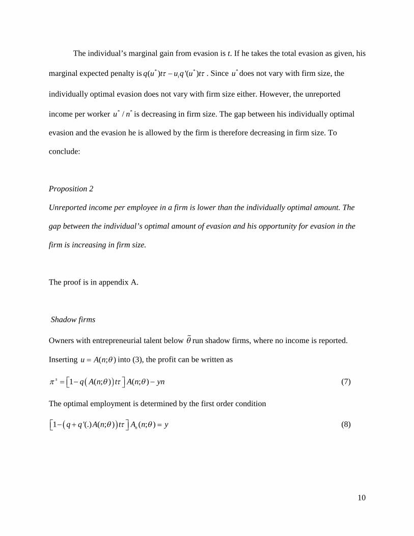
The individual’s marginal gain from evasion is t. If he takes the total evasion as given, his

marginal expected penalty is * *( ) '( )iq u t u q u t . Since *u does not vary with firm size, the

individually optimal evasion does not vary with firm size either. However, the unreported

income per worker * */u n is decreasing in firm size. The gap between his individually optimal

evasion and the evasion he is allowed by the firm is therefore decreasing in firm size. To

conclude:

Proposition 2

Unreported income per employee in a firm is lower than the individually optimal amount. The

gap between the individual’s optimal amount of evasion and his opportunity for evasion in the

firm is increasing in firm size.

The proof is in appendix A.

Shadow firms

Owners with entrepreneurial talent below run shadow firms, where no income is reported.

Inserting ( ; )u A n into (3), the profit can be written as

1 ( ; ) ( ; )s q A n t A n yn (7)

The optimal employment is determined by the first order condition

1 '(.) ( ; ) ( ; )nq q A n t A n y (8)

11

From (8), the demand for labour from a shadow firm can be written as ( , ; )s sn n y t , where sn

is decreasing in y, and t.7

The lower the entrepreneurial talent of the owner, the lower is the profit of his firm.

Individuals with entrepreneurial talent below a critical value 0 cannot run a firm with positive

profit and therefore become employees only.8 The talent 0 of the marginal shadow firm owner

is determined by 0s , i.e.

0 01 ( ; ) ( ; ) 0s s s sq A n t A n yn (9)

Since sn is decreasing in y, and t, 0 is increasing in y and t ,

Labour market equilibrium

Total supply of labour is constant and equal to the total number of individuals, N9. The total

demand for labour is the sum of work hours demanded from registered firms and shadow firms.

As shown above, individuals with talent above 0 become firm owners, those with talent

between 0 and run shadow firms, and those with talent of at least run registered firms.

and 0 are given by (6) and (9). Equilibrium between supply of and demand for labour is then

0 ( , )

*

( , , )

( , , ; ) ( ) ( , ; ) ( )s

y t y t

n y t dFN n y t dF

(10)

7We cannot sign the effect of on employment, but total production goes up as goes up.

8 In our set-up, all individuals supply one unit of labour, whether or not they are firm owners and so all individualsuse alternative cost y on their own labour.9 Alternatively, we might define the supply of labour as the total employee hours, i.e. total work hours N minus thenumber of hours the firm owners work for themselves, i.e. in the firm they own. Correspondingly, total demand isthe sum of the owners’ demand for work hours in excess of their own. In this alternative, total supply of labour is

increasing in w. The equilibrium value*y is of course independent of which of the two definitions we use.

12

We show in appendix A that the total demand for labour is decreasing in the net expected labour

income y. The equilibrium condition (10) determines the net labour income y, which in turn

determines the allocation of labour and thereby the number and size of firms. It also determines

the fraction of shadow firms.

3. A labour market explanation for the tax evasion puzzle

Proposition 1 suggest that it is optimal for employers to ration the unreported work in the firm:

Consequently, the marginal gain from evasion seems higher than the marginal cost for an

individual employee. However, we have shown that the rationing solves the problem that each

individual employee disregards the effect his evasion has on the expected penalty of his fellow

workers. Still, one may ask how such rationing of unreported work can be sustained when the

employees have access to shadow work outside the firm: They may work unreported in the

shadow firms or as self-employed. The reason they may not take these opportunities for shadow

work is that the equilibrium net labour income y is independent of the combination of reported

and unreported work. For example, an employee gains nothing from part time work as employee

in a shadow firm rather than full time in a registered firm. An alternative to work unreported in a

shadow firm is to work unreported as self-employed, i.e. to start up a shadow firm. As self-

employed, the individual’s productivity depends on his own entrepreneurial talent, while his

productivity as an employee depends on the entrepreneurial talent of his employer. The

productivity of a worker employed by a talented owner may be higher than if he runs his own

business. In our model, individuals with entrepreneurial talent below 0 earn more from reported

work for a talented owner, than from unreported work as self-employed.

13

Our model predicts that the average income for those who work unreported is higher than

for those who do not. Again, this is not a puzzle, but easily explained once we distinguish

between labour income and rent on entrepreneurial talent: In equilibrium, individuals who earn

more than the labour income y on unreported work as self-employed do so because their

entrepreneurial talent is high. The higher hourly income of the self-employed is the rent on their

entrepreneurial talent, not a sign that there is a gain from arbitrage in the market for shadow

work.

4. Inefficient labour allocation

With inelastic labour supply, taxes do not distort the allocation of labour if there is no tax

evasion. With tax evasion, however, they do. Tax evasion lowers the marginal cost of labour in

shadow firms and leads to entry of new shadow firms, such that the demand for labour from the

shadow labour market goes up. As a result, labour is reallocated from registered firms to shadow

firms. This reallocation lowers total output since the marginal product of labour is lower in the

shadow firms than in the registered firms.10

The negative effects of on labour allocation is stronger the higher the tax rate. A higher

penalty tax works in the opposite direction. A higher penalty tax makes evasion less profitable,

and as a result more firms register. On the margin, this does not affect the demand for labour.

However, a higher penalty tax also lowers the demand for labour in all shadow firms without

changing the demand for labour from the registered firms. As a consequence, the total demand

10 We cannot determine whether the number of firms goes up or down with tax evasion. On the one hand, taxevasion makes the marginal firm more profitable. On the other hand, the higher labour income y reduces the profit.

14

for labour goes down and leads to a lower equilibrium value of y. The reduction in y leads to

higher employment in registered firms and a higher total output11.

Proposition 3

Tax evasion leads to an inefficient allocation of labour and therefore lower total output. Total

output goes up with a higher penalty tax, and down with a higher tax rate.

The proof is in appendix B.

One implication of Proposition 3 is that taxes create inefficiencies even if there are no distortions

from the taxes themselves. The reason is that taxes encourage tax evasion, which lowers the

marginal cost of labour in the least productive firms.

5. Evidence

In this section we investigate empirically two key predictions of our theoretical model:

Proposition 1 predicts a negative relation between unreported work per employee and the size of

the firm. Proposition 2 predicts that the gap between a worker’s optimal amount of unreported

work and the amount permitted by the employer is increasing in firm size.

Data

The data is taken from two of the Surveys on the Hidden Labour Market (SHLM), which are

surveys of a representative sample of the adult population with focus on unreported work. The

surveys are collected as postal interviews by the Market and Media Institute on behalf of the

11 So far, we have ignored audits based on the individual’s reported income. However, most tax agencies auditindividuals with an income that appears too low, given their observable characteristics. In the appendix we considerthis case, and show that our main results are unaltered.

15

Frisch Centre for Economic Research and the Department of Economics at the University of

Oslo. We use the 1980 and 2003 waves of SHLM since in both of these years employed

respondents are asked about the size of the firm of their regular employment. The response rate

was 73 and 58 percent in 1980 and 2003 respectively. We limit our sample to employed

respondents in the age group between 18 and 64 year of age with valid observations on the

variables used in the analysis.

In the questionnaire the individual is asked about his willingness to receive unreported

income and about his actual unreported work the last 12 months. Two dummy variables,

“Willing” and “Unreported”, are given the value 1 12. In table 1 we show the summary statistics

of these two variables. We note that while there has been a considerable decline in both the

willingness to receive unreported income, and the actual performance of unreported work, the

ratio between willingness and actual performance has increased from 3.1 in 1980 to 5.3 in 2002.

The survey contains information on the human capital variables gender, age, and

educational level. Respondents are also asked about their perceived probability of being detected

if they receive unreported income and to what extent they believe that others accept tax evasion.

We also have information about their pay in their regular job. Several of the variables are

reported in brackets (see table 1), for instance hourly pay. These variables (with the exception of

firm size) are transformed into continuous variables using the midpoints of each bracket. Firm

size is reported in brackets in 1980, and as a continuous variable in 2003. We create dummy

variables according to the 1980-intervals for both years. Summary statistics of the key variables

12 There is a problem of comparing the willingness-answers between the two surveys, since “do not know” was anoption in 2003 but not in 1980. In the empirical analysis, we allocated the “don’t know”-group in 2003 randomly towilling/unwilling to increase comparability between the two years. 50/50 allocation is very close to the proportion inthe 2003 sample that did reveal a preference (51/49). As a robustness check, we have run the all the models reportedin Tables 2 and 4 below, excluding the “don’t know” category in 2003 from the analysis. The results below alsohold when we use this limited sample, with the exception of some of the level comparisons between 2003 and 1980which may obviously be affected. We retain the full sample in the analysis in order to make the comparison betweenthe two years as good as possible. Results for the limited sample are available from the authors on request.

16

in the sample are given in table 1, where we also provide a description of the distribution of

respondents on size categories.

[Table 1 in around here]

The surveys contain several measures of individuals’ norms regarding tax financing and

income inequality, which we will use to identify the “willingness-equation”. In 1980 the

respondents were asked if they agree that the present level of taxes is necessary to finance the

welfare state and if it is understandable that people do unreported work. In 2003 the respondents

were asked if they agree that income inequalities should be small and that income inequalities

due to factors outside one’s own control should be removed. These variables are transformed

into dummy variables, taking the value of 0 in the year they were not asked.

The probability of doing unreported work declines with firm size.

We test proposition 1 by analysing the relationship between the probability that an employed

individual has done unreported work during the last 12 months and the size of the firm where he

has his regular employment. In Table 2, we report the estimated coefficients of probit models of

the probability of having done unreported work. To allow for a flexible specification, we use

dummy variables for each of the firm size categories. Model 1 provides the unconditional size

effect. We find that the probability of unreported work is smaller in larger firms. In particular,

the probability is smaller in firms with more than 10 employees and even smaller in firms with

more than 100 employees. There appears to be a drop in the unconditional coefficient for firms

with more than 500 employees. To show that the size effects are economically significant as well

as statistically significant, figure 1 provides the fraction of employees in the different size

17

brackets that have done unreported work during the last 12-months. These fractions correspond

to the coefficients in model 1 of table 2.

Figure 1. Share of employees who has done unreported work last year

Of course, the raw averages presented in model 1 and figure 1 may be a result of factors we have

not accounted for, such as industry, individual characteristics, probability of detection, norms

and wages. Table 2 provides the result from four additional models where we include these

factors. In model 2 we include industry dummies. In model 3 we include individual

characteristics like gender, age, and education. These factors explain a lot of the variation in

unreported work, but accounting for these factors does not lead to a significant change in the

estimated firm size effects.

[Table 2 around here.]

The size effect could simply be a reflection of the individual’s response to a higher

perceived probability of being detected by the tax agency in larger firms. Furthermore, it is

possible that perceptions of other people’s norms are different in large and small firms. We

control for these factors by introducing subjective measures of the probability of detection and of

0

0.05

0.1

0.15

0.2

0.25

0.3

0.35

1-3 4-6 7-10 11-20 21-50 51-100 101-200 201-500 501+

Firm size (# of employees)

18

the perception of other peoples norms towards tax evasion in model 4. Both the perceived

probability of detection and the beliefs about other peoples’ norms have a strong impact on

actual performance of unreported work, and the signs are as expected. However, the firm size

effect remains even stronger after controlling for these subjective factors. This suggests that there

is no significant correlation between the probability of detection and firm size, a result that is

consistent with the theoretical model where the probability of detection turns out to be equal

across firms in equilibrium. In the last model, we ask the question if the size effect is simply a

direct supply response to higher wages in larger firms. We control for human capital variables

and industry, which also reflect individual productivity. The effect of the hourly wage variable

should therefore be interpreted as conditional on human capital. The individual’s perceived

marginal tax rate is also included in the regression. It turns out that hourly wage has no

significant effect. The marginal tax rate shows up with a negative coefficient. Again, firm size

effects prevail.

There appears to be a pattern in the size coefficients, and tests (not shown) reveal that

there is no significant difference between size groups 1 (the reference group) and group 2,

between size group four, five and six, and between the size groups above 100 employees. We

therefore provide a less flexible specification to increase the degrees of freedom in the model. As

shown in table 3, we can distinguish between the probability of unreported work among

employees in the very small firms (1-6 employees), firms with 7-10 employees, firms between

11 and 100 employees, and the larger firms with more than 100 employees.

[Table 3 around here]

As a robustness check we also present two cuts in the sample. One is a public/private

split and the other is according to the year of observation. We find smaller and less significant

19

effects in the public sector than in the private sector, as well as in 2003 versus 1980. In both of

these sub-samples employees have a much lower probability of doing unreported work

(accounted for industry and year dummies in the pooled specifications). Furthermore, the

patterns revealed by the point estimates are quite similar, and the differences between the sub-

samples are not statistically significant for any of the size ranges. For this reason, and because of

the small share of individuals who do unreported work and the fairly small sample sizes, we

continue to use the pooled specifications.

We have now provided specifications that control for the most relevant supply factors

that should affect the individual’s willingness to do unreported work. Perhaps with the exception

of regular wage and marginal tax, all these variables show up with the expected sign. Still, firm

size has a large effect on the probability of doing unreported work. This result strongly suggests

that the employees’ opportunities for unreported work are smaller in larger firms. However, the

empirical model in this section may be thought of as a reduced form model, and we face a

standard identification problem of distinguishing between the employees’ notional supply and

the actual opportunities for unreported work. In the next section, we try to solve this

identification problem, and thereby also to provide an empirical test of proposition 2 in our

model.

The gap between willingness and actual unreported work

Proposition 2 predicts that the gap between the optimal level of unreported work for the

individual worker and his opportunities for unreported work provided by the employer is

increasing in the size of the firm. In the following we test this proposition, but first we spell out

our empirical strategy.

20

The data give us observations of individuals, not firms. Hence, we have to use variables

related to the employment relation of the workers as firm indicators. As in most empirical studies

in economics, the results in table 2 are not based on separate observations of supply behaviour

and of opportunities (demand) for unreported work, but only on the market outcome. This

implies that we have a standard identification problem. Furthermore, we need to deal with issues

of rationing and selection in our empirical framework, since our model predicts a gap between

the individual’s optimal amount of unreported work in the firm and his opportunities for such

work in the firm. We therefore start by presenting a simple index model of latent supply and of

opportunities based on our theoretical model, and then go on to explain how they are related to

the observations in our data.

Worker i’s latent supply of unreported work is given by ui in our theoretical model. This

is the optimal level of unreported work by the individual, conditional on all other workers

following the employer’s optimal level of evasion within the firm: * */u n . We let this latent

supply be represented by: *s s sy x u where subscript i is suppressed for convenience. The

vector xs includes factors that affect the supply of unreported labour like the perceived

probability of being caught, the punishment for tax evasion, norms and so on. The index function

is normalized such that the worker is willing to supply unreported work if ys* > 0 and unwilling

to supply this kind of work if ys* < 0.

Consider next the opportunities for unreported work for worker i. As detailed in

the theoretical section, employers may rationally restrict their employees’ opportunities for

unreported work. The workers’ opportunities are determined by the firm’s optimal level of

unreported work, divided by the number of workers ( * */u n in our model). As a result of the

externality between workers within the firm, the optimal level of unreported work for the firm is

21

lower than what each individual would prefer for themselves, given the level of unreported work

of all the others being determined by the firm. The firm’s optimal level of unreported work per

employee provides us with an opportunity equation: *d d dy a x b u , where the x vector now

includes factors that influence the agreed wage, like the probability that the firm is caught and

the expected punishment. We use industry indicators as proxies for differences in technology and

organizational design affecting the benefits of using unreported labour. Following proposition 1,

the fraction of workers that is given the opportunity to do unreported work is negatively related

to firm size. The opportunity-equation should therefore include firm size. The firm provides

opportunities for unreported work for worker i, if yd* > 0 and does not provide the opportunities

if yd* < 0.

We assume that E(ui|x) = 0 and Var(ui) = 1 for i= d, s and that Cov(ud, us) = ρ. This

means that we allow for a correlation between the error terms in the two equations. Correlation

may arise from several factors. For instance, we do not observe the implicit wage for unreported

work that would have been realized if the parties had reached an agreement. Stochastic

components of this implicit wage would enter positively into the supply equation and negatively

into the opportunity equation. On the other hand, if “willing” individuals are selected into

occupations where there are more opportunities for unreported work than in other occupations,

there will be a positive component in both error terms, and a positive correlation occurs. The sign

of the correlation is entirely an empirical question, and of course also dependent on what factors

are included in the observed x-vectors.

22

Disentangling the factors determining supply and opportunities

We estimate the indexes of latent supply and opportunities using the following two questions

from the surveys13:

1.“If possible, would you be willing to receive income without reporting it to the tax authorities”

Willing = [Yes, No]

2. “Have you, during the last 12 months, performed work where the income is not (or will not

be) reported to the tax authorities?” Unreported Work = [Yes, No]

If an employee answers “yes” to the question about willingness to receive unreported income,

but “no” to the question about actual performance of unreported work last year, we conclude that

the worker has limited opportunities for unreported work in the firm. We use this assumption to

estimate the gap between the employees’ “supply” of unreported work in the firms, and the

employers’ “demand” for such work.

The first question identifies the parameters of the supply index. The second question

identifies parameters of the opportunity equation, conditional on being willing. There are four

possible outcomes of the two latent variables. However, our data are censored, since we cannot

observe the opportunities for unreported work when the worker is not willing to supply such

work. In our data, we can therefore only distinguish between three situations:

[1] ys > 0 & yd > 0. We find willing (Yes) and unreported work (Yes).

[2] ys > 0 & yd < 0. We find willing (Yes) and unreported work (No).

[3] ys < 0. We find willing (No) and unreported work (No).

Our modelling strategy14 is to use the contrast between situations 1 and 2 to estimate the

opportunity function, and to use the contrast between situations [1, 2] and 3 to estimate the

13 See table 1 for descriptive statistics.14 See Osterbeeck (1998) who uses a similar modelling strategy to analyse the market for firm-provided training.

23

supply function. Since the data are censored, and the two latent equations possibly correlated, we

use a bivariate probit model with selection.

Identification issues

In this section we discuss under what assumptions we can identify the demand- and supply-

equation. First, we need that the answer to the “willing”-question can be used as an indicator of

supply. Clearly, the “willing”-question is too general to represent a direct measure of the

individual’s optimal level of unreported labour supply.15 We demonstrate, however, that it is a

good proxy, by showing that the willingness-indicator responds reasonably to important

determinants of supply, such as the perceived probability of detection, education and norms (see

table 5 below). The problem left is then to what extent the measurement error in willingness is

correlated, conditional on the observed exogenous variables, with firm size. Since the observed

exogenous variables include important supply indicators like the probability of detection, others

norms, and the level of human capital, we do not find it likely that this will be a significant

problem for our estimation procedure. Note also that the results with respect to firm size are

practically unaltered if we include the wage and marginal tax in the equations.16

The next issue is to what extent we are able to identify the parameters of the two

equations, when we use the bivariate probit model with selection that arises from equation (11).

Since we want to estimate the correlation coefficient between the two equations, we also rely on

15 Disregarding the issue of discontinuity arising from the dummy-representation of the dependent variable. Thisproblem is of course easily dealt with using a latent variable interpretation of any standard estimation method forlimited dependent variables, such as the probit model.

16 We have chosen specifications in table 5 without the wage and marginal tax, because they may both beconsidered endogenous in our theoretical model; results including these variables are very similar to those of table 5and are available from the authors on request.

24

some exclusion restrictions. We use four variables reflecting individual norms17 in the

willingness-equation only. This means that our model is not identified by functional form only. If

the correlation coefficient is not significantly different from zero, the most efficient procedure is

to estimate the model by separate probit analyses, identifying the parameters of the supply

equation on the full sample and the parameters of the opportunity equation on the sample of

willing workers only. In table 4 below, we report from both bivariate probit with selection as

well as from separate probit analyses on different samples.

The gap is increasing in firm size

Table 4 presents the results of the estimation of both the willing- and the unreported work-

equations. The first model is a bivariate probit model with selection. Consider the unreported

work equation first. This is now effectively estimated on willing workers only. Again we find

that the probability of doing unreported work is strongly declining in firm size. In model 2 we

show the same result using the same size distribution as in table 3. Consider next the willing-

equation. While displaying significant and reasonable results with respect to the human capital

variables, probability of detection and perception of other peoples’ norms, there is no significant

pattern with respect to firm size. Furthermore, a joint test reveals that there is no significant

effect of firm size and industry on the willingness to supply unreported labour. This result

remains in model 2 as well.

However, since the correlation coefficient between the error terms of the two equations is

not significantly different from zero, the bivariate probit with selection model is unnecessarily

restrictive, and we may simply use separate probit models. The results from these models are

17 The questions reflect attitudes towards the financing of the welfare state as well as towards income inequality. Seethe data section for details.

25

displayed in model 3 in table 4. We find that the separate probit models produce very similar

results to the bivariate probit models. This result is reasonable since the correlation coefficient is

small.

Since willingness is independent of firm size while actual unreported work is negatively

correlated with firm size, the difference between willingness and actual performance of

unreported work is increasing in firm size. We thus conclude that the gap between the

willingness to supply unreported labour and the opportunities provided by the firms is increasing

in firm size.

6. Conclusions

In equilibrium, tax evasion is rationally limited by the employer to lower the joint risk of

detection. At the same time, employees that work unreported as self-employed earn more than

those that do not. This may appear to be a tax evasion puzzle, but it is not. Part of the income as

self-employed is return to entrepreneurial talent. The reason why an individual is self-employed

is that his entrepreneurial talent is high enough to give him a higher income than the normal

return to labour. The reason why some individuals do not take the opportunity to work

unreported as self-employed is that their entrepreneurial talent is not high enough to make self-

employment profitable, even when all income is evaded.

Like many other crimes, tax evasion is more vulnerable when organized, since detecting

one participant may help detect the entire evasion scheme. As a consequence, there is a trade-off

between efficient unreported production and low risk of detection. This efficiency-evasion trade-

off creates a mutually positive relation between tax evasion and small-scale production: Tax

evasion per worker is higher in small unproductive firms than in large productive ones. At the

26

same time, tax evasion increases the demand for labour in low-productive shadow firms, causing

an inefficient allocation of labour with too low employment in high-productive firms. A policy

implication is that even taxes that are non-distortive with no tax evasion, create distortions in the

presence of tax evasion.

In the empirical part, we test two key predictions of the theoretical model: First, that

unreported work per employee is decreasing in firm size. Second, that there is a gap between the

employees’ willingness to work unreported and their opportunities for such work in the firm, and

that this gap is increasing in firm size. Using survey data, we find support for both predictions:

First, an employee’s probability of doing unreported work is declining in firm size. Second, there

is a gap between the employees’ willingness to receive unreported income and their actual

performance of unreported work. This gap is increasing in firm size. We take these two results as

evidence that employers limit the opportunities for tax evasion among their employees. They

also offer support to our analysis of market behaviour and the allocation of talent.

References:

Allingham, M.G. and A. Sandmo,(1972). “Income Tax Evasion: A Theoretical Analysis.”

Journal of Public Economics 1, pp.323-338.

Alm, J.,I. Sanchez and A.De Juan (1995), “Economic and noneconomic factors in tax

compliance” KYKLOS, 48. pp3-18.

Boeri, T. and P.Garibaldi (2006), “Shadow sorting”, CEPR Discussion Papers 5487, February

2006.

Dhami,S. and A. al-Nowwaihi (2007), “Why do people pay taxes?”, Prospect theory versus

expected utility theory”, Journal of Economic Behavior and Organization, Vol.64, 171-192.

27

Cowell, F. A.(1981), “Tax evasion with labour income”, Journal of Public Economics, 26,

pp.19-34.

De Paula,A. and J.A.Sheinkman, (2008), “The informal sector”, PIER Working Paper, 08-018.

Fortin,B.,G.Lacroix and M.C.Villeval, (2004),” Tax evasion and social interactions”, Working

paper 04-10, Groupe d’Analyse et de Theorie Economique, Centre National de la Recherche

Scientifique.

Fugazza, M. and J.F. Jacques (2003), “Labour market institutions, taxation and the underground

economy”, Journal of Public Economics 88, pp.395-418.

Goldstein, H.,Hansen,W.G., Ognedal,T., og S.Strøm, S. (2002), ”Svart arbeid fra 1980 til 2001”,

(Unreported work from 1980 to 2001), Frisch-Rapport 3/2002.

Kolm, A.S. and Nielsen, S.B.(2008), “Under-reporting of income and labor market

performance”, Journal of Public Economic Theory, Vol. 10, No. 2, p. 195-217

Murphy, K.M., Shleifer, A.and R.W.Vishny, (1991), “The allocation of talent: Implications for

growth”, The Quarterly Journal of Economics, vol.106, No.2, pp.503-530.

Oosterbeek, H., (1998),”Unravelling the demand and supply for firm provided training”, Oxford

Economic Papers 50, pp. 266-283.

Pestieau, P. and U.M.Possen (1991),”Tax evasion and occupational choice”, Journal of Public

Economics 45, pp.107-125.

Sandmo, A. (1981), “Income tax evasion, labour supply, and the

efficiency-equity tradeoff,” Journal of Public Economics 16, 265-288.

Tonin, M.(2007),” Minimum wage and tax evasion: Theory and evidence”, Hungarian Academy

of Sciences, Institute of Economics, 2007; Working Paper 2007/01

28

Appendix A: Proof of proposition 2

Let iu denote the unreported income of individual i. Using (2), the net expected income of

individual i can be written as

1

(1 ) 1 ( )n

i i jj

I t w u q u t

Leaving one more dollar of his gross income w u unreported, i.e. decreasing w and increasing

u yields

1 (.) '(.)ii

i

dIt q u q

du (A.1)

Rearranging the firm’s first order condition (7) yields

** * * * *

* *

1 11 ( ) '( ) '( ) 0

nq u u q u u q u

n n

(A.2)

Using this to evaluate (A.1) at the optimum * *,u n yields

* **

* *

1'( ) 0i

i

dI u nq u t

du n n

(A.1)΄

The individual employee would benefit from reporting less of his income for taxation. The

reason is that he does not take into account the increased expected penalty that he inflicts on the

1n other employees by leaving more income unreported.

29

Appendix B: Proof of proposition 3

It is immediate from (5), (6) and (7) that higher penalty taxes ( ) reduces tax evasion. Tax

evasion is lower in both registered firms and ghosts and fewer ghosts survive. We prove that this

leads to higher total output. The total output in the economy is

0

*( ; ) ( ) ( ; ) ( )sY A n dF A n dF

(B.1)

Differentiating with respect to yields

0

0 *0 0 0 *( ; ) ( ) ( ) ( )

sg

n n

dY d dn dnA n f A dF A dF

d d d d

(B.2)

where0

0 0y

dy

d

,

ss s

y

dnn n y

d

and

**

y

dnn y

d

.

From (9) we get1 ( )

sn

yA

h

, where ( ) '( ( ; )) ( ; )h qt q A n t A n and

from (6)′ we get *

1n

yA

t

. Since the profit of the marginal firm, a ghost, is zero, we get

0 0 0

0( ; )

1

yA n n

q t

. Inserting for 0 0( ; )A n , s

nA and *nA in (B.2) and rearranging, we can write

(B.2) as

0

0 *0 0

0

1 1( ) ( ) ( )

1 1 1 ( )

sdY y d t t dn dnn f dF dF

d t d q t h d d

(B.2)′

Differentiating (10), the equilibrium condition for the labour market, with respect to yields

0

0 *0 0( ) ( ) ( ) 0

sd dn dnn f dF dF

d d d

(B.3)

30

Since*

* 0y

dn dyn

d d , the last term in (B.3) is positive and the sum of the first two terms must

be negative. Compare with (B.2)′, which is a weighted sum of the three terms in (B.3). Since

both weighs in (B.2)′ are less than one,the two negative terms are given reduced weight

compared to (B.3). This implies that the sum of the three terms in (B.2)′ must be positive, i.e.

0dY

d .

To prove the last part of proposition 3, that higher taxes reduce total output, we

differentiate Y with respect to t. This yield

0

0 *0 0 0 *( ; ) ( ) ( ) ( )

sg

n n

dY d dn dnA n f A dF A dF

dt dt dt dt

(B.4)

Where0

0 0t y t

dy

dt

,

gg g

t y t

dnn n y

dt and

** *

t y t

dnn n y

dt .

Using that1 ( )

sn

yA

h

, *

1n

yA

t

and 0 0 0

0( ; )

1

yA n n

q t

we can rewrite (B.4) as (B.4)′

0

0 *0 0

0

1 1( ) ( ) ( )

1 1 1 ( )

sdY y d t t dn dnn f dF dF

dt t dt q t h dt dt

Equilibrium in the labour market requires that the total demand for labour is unchanged by the

increase in t, which gives us

0

0 *0 0( ) ( ) ( ) 0

sd dn dnn f dF dF

dt dt dt

(B.5)

Comparing (B.4)′ and (B.5), dY/dt is a weighted sum of the three terms in (B.5), where the first

two terms have weights lower than one. To show that dY/dt is negative, we show that dn*/dt<0.

Differentiating (6)′ with respect to t yields

31

* 1

(1 ) 1nn

dn dy y

dt t A dt t

(B.6)

To sign dn*/dt, we need to find the size of dy/dt. Differentiating of the labour equilibrium

condition with respect to t gives us

0

1 2 30

( ' )( ) ( )

1 1 ( ) 1

dy y y q q A ydF dF

dt q t h t

(B.7)

Where0 0 0

1

( ) y

Dy

n f

N

, 2

sy

Dy

n

N and

*

3

y

Dy

n

N . The right hand side is

Dt

Dy

N

N. Since

0

1 2 3( ) ( ) 1dF dF

, it follows that1

dy y

dt t

, which from (B.6) implies that

*

0dn

dt . Since dY/dt is a weighted sum of the three terms in (B.5), where the first two terms

have weights lower than one, it follows that when*

0dn

dt , 0

dY

dt . Q.e.d.

32

Table 1a. Summary statisticsAll 1980 2003

Willingto take unregisteredincome (dummy variable)

0.65 0.72 0.58

Unregstered work last 12months(dummy variable)

0.16 0.23 0.11

Year 1980(dummy variable)

0.44 1 0

Woman(dummy variable)

0.43 0.36 0.47

Probability of detection(midpoints of brackets)

0.37 0.33 0.40

Tax evasion generally acceptedby others(dummy variable)

0.87 0.84 0.89

Experience(years)

22.28 21.16 23.16

High School(dummy variable)

0.30 0.22 0.44

College +(dummy variable)

0.34 0.21 0.36

log hourly wage(midpoints of brackets)

4.90 4.77 5.01

Marginal Tax rate(midpoints of brackets)

44.21 49.39 40.12

N 1107 488 619

33

Table 1b. Size distribution. Employees in 1980 and 2003

Number of employees in firm 1980 20031-3 11.48 10.024-6 6.76 10.827-10 6.76 7.5911-20 11.89 14.7021-50 19.88 19.7151-100 9.63 13.41101-200 10.25 7.92201-500 9.63 7.27501+ 13.73 8.56

34

Table 2. Unreported work last 12 months. Employees.Probit models.

Model1 Model2 Model3 Model4 Model5Year 1980 0.5318*** 0.5874*** 0.4060*** 0.3911*** 0.4968***

(0.0945) (0.1014) (0.1209) (0.1245) (0.1421)size 4-6 -0.1854 -0.2371 -0.2040 -0.2657 -0.2353

(0.1881) (0.1925) (0.2013) (0.2077) (0.2095)size 7-10 -0.4486** -0.4838** -0.4735** -0.5546** -0.4959**

(0.2099) (0.2204) (0.2294) (0.2379) (0.2396)size 11-20 -0.5138*** -0.5539*** -0.5961*** -0.6801*** -0.6371***

(0.1783) (0.1874) (0.1960) (0.2027) (0.2051)size 21-50 -0.5436*** -0.5645*** -0.5876*** -0.6409*** -0.5908***

(0.1626) (0.1737) (0.1807) (0.1852) (0.1876)size 51-100 -0.5316*** -0.5646*** -0.5208** -0.6329*** -0.5731***

(0.1862) (0.1961) (0.2027) (0.2090) (0.2116)size 101-200 -0.7500*** -0.8372*** -0.8063*** -0.9248*** -0.8531***

(0.2102) (0.2222) (0.2302) (0.2380) (0.2400)size 201-500 -0.9681*** -0.9034*** -0.8675*** -0.9708*** -0.9031***

(0.2325) (0.2429) (0.2509) (0.2590) (0.2622)size > 500 -0.5792*** -0.6885*** -0.6487*** -0.7385*** -0.6470***

(0.1879) (0.2027) (0.2108) (0.2177) (0.2214)Woman -0.7002*** -0.6181*** -0.6970***

(0.1242) (0.1286) (0.1348)Age -0.0231*** -0.0188*** -0.0168***

(0.0046) (0.0048) (0.0049)College education -0.3157** -0.4183*** -0.3591**

(0.1583) (0.1612) (0.1732)High-school 0.0244 -0.0619 -0.0227

(0.1331) (0.1366) (0.1387)Prob. of detection -1.0728*** -1.0808***

(0.2642) (0.2657)Generally accepted 0.7290*** 0.7585***

(0.2175) (0.2202)log(hourly wage) -0.0365

(0.1852)Marginal tax rate -0.0098*

(0.0050)Industry dummies N Y Y Y YConstant -0.7829*** -0.6231*** 0.5318* 0.1376 0.5320

(0.1329) (0.1769) (0.2949) (0.3702) (0.8656)N 1107 1107 1107 1107 1107* Standard error in parenthesis. Significance levels (*) 0.10, (**)0.05, and (***) 0.01

35

Table 3. Unreported work last 12-months.Coefficients for size in different samples. Probit models

All Private Public Y1980 Y2003Size 7-10 -0.3948* -0.3412 -0.5383 -0.4478 -0.3488

(0.2217) (0.2496) (0.5621) (0.3358) (0.3130)Size 11-100 -0.4985*** -0.4787*** -0.5761 -0.6347*** -0.4409**

(0.1372) (0.1499) (0.4009) (0.2144) (0.1885)Size > 100 -0.6791*** -0.6728*** -0.6726 -0.9732*** -0.4200*

(0.1608) (0.1810) (0.4196) (0.2386) (0.2353)N 1107 756 308 488 588

Note: Standard error in parenthesis All models also include the samecovariates as in Table 1. Significance levels (*) 0.10, (**) 0.05, and (***)0.01

36

Table 4. Unreported work and the willingness to take unreported income

Dependent Unreported work last 12 monthsSample All Sample of willingMethod Bivariate probit with selection Probitsize 4-6 -0.3693

(0.2323)size 7-10 -0.6209**

(0.2634)size 11-20 -0.7735***

(0.2253)size 21-50 -0.7450***

(0.2122)size 51-100 -0.7401***

(0.2365)size 101-200 -1.0116***

(0.2603)size 201-500 -1.1306***

(0.2867)size > 500 -0.8706***

(0.2445)Size 7-10 -0.4576* -0.4302*

(0.2428) (0.2472)Size 11-100 -0.5837*** -0.5990***

(0.1508) (0.1495)Size > 100 -0.8151*** -0.8316***

(0.1743) (0.1727)Woman -0.5962*** -0.6091*** -0.5842***

(0.1376) (0.1369) (0.1396)Age -0.0173*** -0.0171*** -0.0158***

(0.0052) (0.0051) (0.0051)College education -0.3556* -0.3457* -0.2855

(0.1822) (0.1797) (0.1746)High-school -0.0371 -0.0088 0.0079

(0.1469) (0.1452) (0.1465)Prob. of detection -0.9469*** -0.9429*** -0.7745***

(0.3313) (0.3274) (0.2991)Generally accepted 0.5398* 0.5364* 0.4012

(0.2855) (0.2835) (0.2583)Size&Industry, p-value 0.004 0.0000 0.0000# of censored 393 393 -N 1107 1107 714

ρ(Unrep.,Willing) 0.3388 0.3481 (0.4025) (0.3951)

37

Table 4. continuedDependent Willing to take unreported incomeSample AllMethod Bivariate probit with selection Probitsize 4-6 0.1011

(0.1965)size 7-10 -0.1916

(0.2063)size 11-20 -0.0484

(0.1786)size 21-50 0.1471

(0.1688)size 51-100 0.1631

(0.1851)size 101-200 -0.0773

(0.1962)size 201-500 0.1845

(0.2043)size > 500 0.0959

(0.1962)Size 7-10 -0.2413 -0.2313

(0.1871) (0.1865)Size 11-100 0.0454 0.0517

(0.1232) (0.1228)Size > 100 0.0123 0.0201

(0.1366) (0.1361)Woman -0.3066*** -0.3095*** -0.3078***

(0.0980) (0.0977) (0.0975)Age -0.0141*** -0.0138*** -0.0136***

(0.0039) (0.0039) (0.0039)College education -0.5583*** -0.5363*** -0.5323***

(0.1321) (0.1305) (0.1310)High-school -0.1738 -0.1745 -0.1761

(0.1215) (0.1209) (0.1211)Prob. of detection -1.3032*** -1.3026*** -1.2873***

(0.1934) (0.1927) (0.1914)Generally accepted 0.7328*** 0.7417*** 0.7411***

(0.1310) (0.1303) (0.1304)Norms p-value 0.0000 0.0000 0.0000Size&Industry, p-value 0.5580 0.4850 0.4914N 1107 1107 1107

Note: Standard error in parenthesis. All models include industry dummies.