Environmental noise beside an elevated box girder bridge ...

Wenluo Yu & Jian Kang: Environmental Planning and Management [DOI:10.1080/09640568.2018.1427560]
Environmental Planning and Management , Volume 61, Feb 2018, Pages 1–25 Page1
Resistance of villages to elevated-road traffic noise Wen Luo Yua, Jian Kanga,b,*
a Heilongjiang Cold Region Architectural Science Key Laboratory, School of Architecture, Harbin Institute of
Technology, No.66, Xidazhi Street, Nangang District, Harbin, China;
b School of Architecture, University of Sheffield, Western Bank, Sheffield S10 2TN, United Kingdom
* Corresponding author.
Abstract
The purpose of this study is to evaluate the methods of reducing elevated-road traffic-noise levels in rural residential areas by controlling the relative locations and morphological parameters and to investigate the effect of noise barriers on noise attenuation along elevated roads and building facades in villages. This study selected six morphological parameters and used noise-mapping techniques to estimate the noise attenuation in 60 village sites. The results indicate that ‘quiet areas’ increase by approximately 10% for each additional 100 m increase in the distance between the elevated road and the village. The best strategy for noise reduction is keeping the elevated road 1,000 m away from the village and raising the road height to 20 m. The building façade conditions only affect the traffic noise level attenuation when the buildings are within 100 m of the elevated road. It was found that the cost-effective length of the road noise barrier is 600 m on both sides of the village parallel to the road. The results highlight the importance of using morphology to improve the traffic noise resistance of villages. The landscape shape indices of buildings and roads are the most important parameters that affect the traffic noise attenuation of elevated roads.
Keywords: Elevated road; Village; Morphology; Noise attenuation; Traffic noise
2018 Environmental Planning and Management
Date Received: 17 May 2017 Date Accepted: 11 Dec 2017
Published online: 15 Feb 2018.
1. Introduction
People's health and standard of living are significantly affected by the acoustic
properties of their living environment (Sobotova et al., 2010; Fritschi et al. 2011).
Thus, traffic noise is a public hazard that causes harm to the masses because of its
large area of influence and long action time (Ko et al., 2011). With the acceleration
of urban and rural integration processes in China, traffic systems between rural and
urban areas have improved. Villages are rural residential areas where villagers live
and engage in all types of production activities. Hence, it is important to address the
serious problem of disturbance to villagers due to traffic noise (He and Kang, 2014;
Wenluo Yu & Jian Kang: Environmental Planning and Management [DOI:10.1080/09640568.2018.1427560]
Environmental Planning and Management , Volume 61, Feb 2018, Pages 1–25 Page2
Meng and Kang, 2014; Murthy et al., 2010; Rey Gozalo, BarrigónMorillas, and
Gómez Escobar, 2012; Rey et al., 2013; Xi, et al., 2015; Yari, et al., 2016).
To solve the problems related to traffic, ecology, geology, land resources, etc.,
elevated roads are preferred for inter-city traffic (Li and Yang, 2013; Liu, 2008;
Wang and Kang, 2011; Wu, 1998). However, raising the sound source position will
enlarge the noise diffusion area (Zhang, 2004), which inevitably aggravates the
traffic noise pollution along these elevated roads (Chen et al., 2007; Yang, 2016; Ye ,
Xia and Hu, 2016). To reduce traffic noise and increase the proportion of quiet areas,
various solutions have been suggested: solutions based on road traffic volume,
vehicle speed, and surface materials (Avsar and Gonullu, 2005; Li, Zhu, and Sun,
2007); those based on predictions of noise from elevated roads by using noise map
techniques (Chen and Xiong, 2013; Li, Li and Li., 2012; Sun, Liu, and Wang, 2010;
Zhang, 2014); controlling the propagation of traffic noise from elevated roads by
using sound barriers (Ma and Li, 2009; Mei, Kang and Huang, 2016; Wang and Gai,
2012; Yu, 2008; Yu and Gao, 2013); using urban forms such as the influence of
morphological parameters (Hao et al., 2015; Liu et al., 2014; Salomons and Pont,
2012); and improving the properties of buildings affected by the noise, e.g. through
the design of architectural monomers (Kim and Kim, 2007; Wong et al., 2010; Yang
Kang, and Choi, 2012).
Rural areas are significantly affected by the natural environment. Owing to the lack
of professional guidance, the layout planning of buildings in rural areas is rather
haphazard (Zhang and Yin, 2014). Because of high construction cost, buildings in
rural areas are generally low-rise types, and their numbers have been growing
rapidly (Shao, Jin, and Zhao, 2016; Wang, 2014). As previously mentioned (Chen et
al., 2007; Chen and Xiong, 2013; Li , Li and Li., 2012; Ma and Li, 2009; Mei, Kang,
and Huang, 2016; Sun, Liu and Wang, 2010; Wang and Gai, 2012; Yang, 2016; Ye,
Xia and Hu, 2016; Yu, 2008; Yu and Gao, 2013; Zhang, 2004; Zhang, 2014), the
numerous research results aimed at reducing noise along elevated roads in cities and
towns are not entirely applicable to the village environment owing to economic
constraints; however, there are even fewer studies on the subject of improving the
resistance of villages to elevated-road traffic noise.
Therefore, this study aims to examine the influence of distance between villages and
elevated roads, the height and sound barriers of elevated roads, and the materials of
building facades in villages. It also aims to explore methods of integrating the effects
of urban morphological parameters to improve the traffic noise resistance and create

Wenluo Yu & Jian Kang: Environmental Planning and Management [DOI:10.1080/09640568.2018.1427560]
Environmental Planning and Management , Volume 61, Feb 2018, Pages 1–25 Page3
more quiet environments in rural residential areas in China (Hao and Kang, 2014;
Lam et al., 2013; Wang and Kang, 2011). To analyse these parameters, a sequential
noise mapping was performed for the selected typical villages.
2. Methodology
2.1. Selection of sample village sites
In this study, 60 villages in the Sanjiang and Songnen Plain in Heilongjiang (Fig. 1a)
- the severely cold area and northernmost province of China - were selected because
of their unique geographical location, variety of natural reserves, large
peasant population, and the prominence of the plain area in Heilongjiang as a
major grain-producing area according to the Heilongjiang Statistical Yearbook
(2014). As shown in Fig. 1b, Heilongjiang has a transportation network comprising a
motorway/elevated road and hierarchical traffic roads throughout the province. It has
a plentiful river system: large rivers Heilong Jiang, Songhua Jiang, Wusuli Jiang,
and Suifenhe. Moreover, many small-scale rivers have anastomosing reaches, where
many viaducts are built, most of them for motorways that generate widespread traffic
noise. Sixty research samples were chosen from Sanjiang Plain (Shuangyashan S1 to
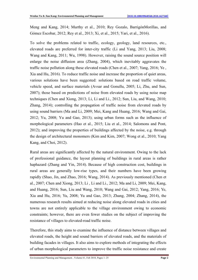
S14 and Kiamusze K1 to K16) and Songnen Plain (Harbin H1 to H30). Fig. 2 shows
the serial numbers of the villages, range of the studied areas of the village, and the
positional relationship between the villages and virtual (designed) elevated road (Yu
and Kang, 2016; Yu and Kang, 2017). The red lines representing the range of the
studied areas of the village indicate the area enclosed by expanding the building zone
of the villages and the outside edge line of the road by 20 m.
(a)

Wenluo Yu & Jian Kang: Environmental Planning and Management [DOI:10.1080/09640568.2018.1427560]
Environmental Planning and Management , Volume 61, Feb 2018, Pages 1–25 Page4
(b)
Figure 1. Locations of the study sites. (a) Contour map of Heilongjiang. (b) Roads and rivers in
Heilongjiang.
2.2 Selection of morphological parameters
This study used previous research as a reference (Burian, Han, and Brown, 2005;
Hao et al, 2015; Oke, 1988; Yu and Kang, 2016; Yu and Kang, 2017) and explored,
developed, and used 12 morphological parameters to describe the characteristics of
village forms in severely cold areas and comprehensively summarised the potential
influencing factors of outdoor sound propagation such as geometric divergence,
ground effects, canyon effect, and barrier effect (Kang, 2007). The building plan
area fraction (BPAF), complete aspect ratio (CAR), landscape shape index of
buildings (LSI_B), and patch density (PD) were mainly related to barrier attenuation,
screening, and reflection. The landscape shape index of roads (LSI_R), road length
fraction (RLF), distance of first-row building from the road (DFBR), and
height-to-width ratio (HWR) were mainly related to geometric divergence, ground
effects, and canyon effect. The edge density (ED), road intersections fraction (RIF),
T-ratio (TR), and cell ratio (CR) were mainly associated with the village planning
forms (Table 1) (Yu and Kang, 2016; Yu and Kang, 2017).
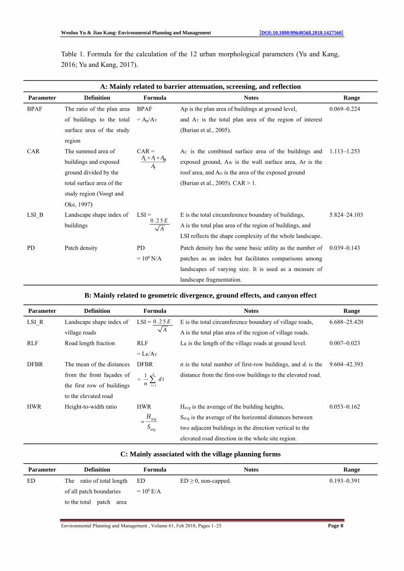
The morphological parameters of the villages failed to satisfy the mutually
independent statistical properties (Table 2) (Yu and Kang, 2016; Yu and Kang,
2017). Therefore, the method of factor analysis with equamax rotation was applied
for screening and reducing the parameters. Four factors were identified which can
explain approximately 88.14% of the variation in the 12 parameters (Table 3). In

Wenluo Yu & Jian Kang: Environmental Planning and Management [DOI:10.1080/09640568.2018.1427560]
Environmental Planning and Management , Volume 61, Feb 2018, Pages 1–25 Page5
Wenluo Yu & Jian Kang: Environmental Planning and Management [DOI:10.1080/09640568.2018.1427560]
Environmental Planning and Management , Volume 61, Feb 2018, Pages 1–25 Page6

Wenluo Yu & Jian Kang: Environmental Planning and Management [DOI:10.1080/09640568.2018.1427560]
Environmental Planning and Management , Volume 61, Feb 2018, Pages 1–25 Page7
Figure 2. CAD image of the village sites based on Google Maps. Scale = 1:1000. S, K, and H are
the abbreviation for city names where the village sites are located. The range of the studied areas
of the village is shown in red lines; Elevated roads are coloured green, buildings are coloured blue,
and roads are coloured black (Yu and Kang, 2016; Yu and Kang, 2017).
addition, an SRC analysis based on nonparametric estimation (He and Zhang, 2009)
was used to examine the sensitivity of various parameters to the influence of
subordinate common factors. Finally, the parameters that have higher absolute
values of sensitivity coefficients are determined and retained from each factor, that is
factor I: CAR and PD, factor II: LSI_B and LSI_R, factor III: RIF, and factor IV:
RLF. The following six representative parameters that could objectively reflect the
form of villages in severely cold areas were selected: CAR, LSI_B, PD, RLF, RIF,
and LSI_R (Yu and Kang, 2016; Yu and Kang, 2017).
Wenluo Yu & Jian Kang: Environmental Planning and Management [DOI:10.1080/09640568.2018.1427560]
Environmental Planning and Management , Volume 61, Feb 2018, Pages 1–25 Page8
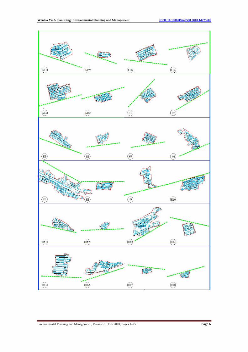
Table 1. Formula for the calculation of the 12 urban morphological parameters (Yu and Kang,
2016; Yu and Kang, 2017).
A: Mainly related to barrier attenuation, screening, and reflection
Parameter Definition Formula Notes Range
BPAF The ratio of the plan area
of buildings to the total
surface area of the study
region
BPAF
= Ap/AT
Ap is the plan area of buildings at ground level,
and AT is the total plan area of the region of interest
(Burian et al., 2005).
0.069–0.224
CAR The summed area of
buildings and exposed
ground divided by the
total surface area of the
study region (Voogt and
Oke, 1997)
CAR =
AC is the combined surface area of the buildings and
exposed ground, AW is the wall surface area, Ar is the
roof area, and AG is the area of the exposed ground
(Burian et al., 2005). CAR > 1.
1.113–1.253
LSI_B Landscape shape index of
buildings
LSI = E is the total circumference boundary of buildings,
A is the total plan area of the region of buildings, and
LSI reflects the shape complexity of the whole landscape.
5.824–24.103
PD Patch density PD
= 106 N/A
Patch density has the same basic utility as the number of
patches as an index but facilitates comparisons among
landscapes of varying size. It is used as a measure of
landscape fragmentation.
0.039–0.143
B: Mainly related to geometric divergence, ground effects, and canyon effect
Parameter Definition Formula Notes Range
LSI_R Landscape shape index of
village roads
LSI = E is the total circumference boundary of village roads,
A is the total plan area of the region of village roads.
6.688–25.420
RLF Road length fraction RLF
= LR/AT
LR is the length of the village roads at ground level. 0.007–0.023
DFBR The mean of the distances
from the front façades of
the first row of buildings
to the elevated road
DFBR n is the total number of first-row buildings, and di is the
distance from the first-row buildings to the elevated road.
9.604–42.393
HWR Height-to-width ratio HWR Havg is the average of the building heights,
Savg is the average of the horizontal distances between
two adjacent buildings in the direction vertical to the
elevated road direction in the whole site region.
0.053–0.162
C: Mainly associated with the village planning forms
Parameter Definition Formula Notes Range
ED The ratio of total length
of all patch boundaries
to the total patch area
ED
= 106 E/A
ED ≥ 0, non-capped.
0.193–0.391
w r G
T
A A A
A
&
0 .2 5 E
A
0 .2 5 E
A
avg
avg
H
S
1
1 n
i
d in
Wenluo Yu & Jian Kang: Environmental Planning and Management [DOI:10.1080/09640568.2018.1427560]
Environmental Planning and Management , Volume 61, Feb 2018, Pages 1–25 Page9
RIF Road intersections
fraction
RIF
= NI/AT
NI is the total number of road intersections,
AT is the total plan area of the region of interest,
0.125–1.506
CR Cell ratio
(Stephen, 2004)
CR NCE is total number of cells and NCU is the total number
of cul-de-sacs.
0.000–1.000
TR T-ratio
(Stephen, 2004)
TR
= NT/NI
NT is the total number of T-junctions and
NI is the total number of intersections.
0.000–1.000
Table 2. Spearman’s rho correlations between urban morphological parameters (2-tailed). Significant correlations
are marked with * (p < 0.05) and ** (p < 0.01) (Yu and Kang, 2016; Yu and Kang, 2017).
BPAF CAR LSI_B PD ED RLF CR TR RIF LSI_R DFBR HWR
BPAF 1
CAR .602** 1
LSI_B 1
PD .323* .840** 1
ED -.709** .299* 1
RLF .337** .323* 1
CR .573** 1
TR .295* -0.066 -.326* -.371** -.276* 1
RIF .309* .804** .599** 1
LSI_R .842** .297* .337** -.403** 1
DFBR -.297* -.388** 1
HWR .622** .768** .601** -.392** -.411** 1
* p < 0.05 (2-tailed)
** p < 0.01 (2-tailed)
Table 3. The results of the factorial analysis.
Factors Parameters Explained
(%) Factor I CAR, BPAF, PD, ED, and DFBR 33.91
Factor II LSI_B, LSI_R, and HWR 28.46
Factor III RIF, CR, and TR 15.75
Factor IV RLF 10.02
2.3 Noise map
To simulate the propagation and attenuation of traffic noise in villages in severely
cold areas, noise maps were calculated with a commonly used noise-mapping
package Cadna/A in this study [DataKustik, 2006]. The speed was taken into
account according to the chosen standard, RLS 90. The measurement speed and
CE
CE CU
N
N N
Wenluo Yu & Jian Kang: Environmental Planning and Management [DOI:10.1080/09640568.2018.1427560]
Environmental Planning and Management , Volume 61, Feb 2018, Pages 1–25 Page10
speed limit were between 40 km/h and 80 km/h for trucks, and 60 km/h and 100
km/h for cars. The design speed was 80 km/h for trucks and 100 km/h for cars. The
calculation was based on the calculation of road traffic noise model for roads, with
values embedded in the software package, Cadna/A. The accuracy of the calculation
was validated using the measurements obtained from villages in severely cold areas,
although calculation errors were relatively higher at few measuring points, which
were far away from the sound source. The average calculation error was less than 2
dBA (Mei, 2014; Meng, 2014). The sound absorption coefficient of the buildings
was set as 0.2, the number of times the propagated sound was reflected was set as 2,
the height of the receiving point was set as 1.5 m, and the grid size of the analogy
computation was set as 10 m × 10 m (Meng and Kang, 2014; Yu and Kang, 2016;
Yu and Kang, 2017).
Through field research, it was found that the majority of buildings in the villages in
Heilongjiang Province are one-story buildings with pitched roofs (Shao, Jin and
Zhao, 2016), indicating a typical, low-rise residential rural morphology. To reduce
the time required for model construction and calculation, pitched roofs were
simplified into flat roofs in the modelling. Therefore, it was necessary to increase the
height of the eaves by 0.7 m and establish a model according to the building height
of 4.5 m (Kang, 2007; Mei and Kang, 2014; Meng and Kang, 2014; Yu and Kang,
2016; Yu and Kang, 2017). Elevated roads comprise a series of bridges that are 6 m
above the ground (net height including the structural height of the bridge). Table 4
shows the scenarios of the study in detail. When studying the reflection of sound
from the building facades on the sound environment, this study compared and
simulated the influence of two types of building facades. One type of building facade
was composed of smooth hard materials (expressed as R3). The other type of
building facade was composed of rough materials with a greening function or a good
sound absorption effect (expressed as R0). The number of reflections for the
simulation analysis of R3 and R0 was set as 3 and 0, respectively, and the sound
absorption coefficient of the building facades was set as 0.1 and 0.9, respectively
(Hao and Kang, 2014; Kang, 2007). The traffic volume per day of the motorway and
rural road conform to the ‘Design Specification for Highway Alignment’ (JTG
D20-2006). In this study, the traffic volume rates of the elevated road were set as
30,000 vehicles per day. If the traffic flow were doubled, the sound pressure level
would increase by 3 dBA (Avsar and Gonullu, 2005). Based on previous research
results (Meng and Kang, 2014; Hao et al., 2015; Yu and Kang, 2016; Yu and Kang,
2017), this study divided the evaluation of sound pressure in outdoor spaces in the
Wenluo Yu & Jian Kang: Environmental Planning and Management [DOI:10.1080/09640568.2018.1427560]
Environmental Planning and Management , Volume 61, Feb 2018, Pages 1–25 Page11
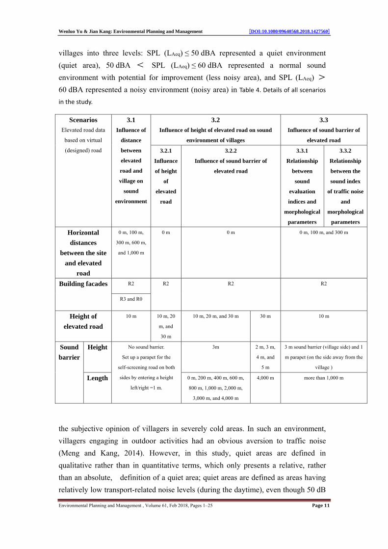
villages into three levels: SPL (LAeq) ≤ 50 dBA represented a quiet environment
(quiet area), 50 dBA < SPL (LAeq) ≤ 60 dBA represented a normal sound
environment with potential for improvement (less noisy area), and SPL (LAeq) >
60 dBA represented a noisy environment (noisy area) in Table 4. Details of all scenarios
in the study.
Scenarios
Elevated road data
based on virtual
(designed) road
3.1
Influence of
distance
between
elevated
road and
village on
sound
environment
3.2
Influence of height of elevated road on sound
environment of villages
3.3
Influence of sound barrier of
elevated road
3.2.1
Influence
of height
of
elevated
road
3.2.2
Influence of sound barrier of
elevated road
3.3.1
Relationship
between
sound
evaluation
indices and
morphological
parameters
3.3.2
Relationship
between the
sound index
of traffic noise
and
morphological
parameters
Horizontal
distances
between the site
and elevated
road
0 m, 100 m,
300 m, 600 m,
and 1,000 m
0 m 0 m 0 m, 100 m, and 300 m
Building facades R2 R2 R2 R2
R3 and R0
Height of
elevated road
10 m 10 m, 20
m, and
30 m
10 m, 20 m, and 30 m 30 m 10 m
Sound
barrier
Height No sound barrier.
Set up a parapet for the
self-screening road on both
sides by entering a height
left/right =1 m.
3m 2 m, 3 m,
4 m, and
5 m
3 m sound barrier (village side) and 1
m parapet (on the side away from the
village )
Length 0 m, 200 m, 400 m, 600 m,
800 m, 1,000 m, 2,000 m,
3,000 m, and 4,000 m
4,000 m more than 1,000 m
the subjective opinion of villagers in severely cold areas. In such an environment,
villagers engaging in outdoor activities had an obvious aversion to traffic noise
(Meng and Kang, 2014). However, in this study, quiet areas are defined in
qualitative rather than in quantitative terms, which only presents a relative, rather
than an absolute, definition of a quiet area; quiet areas are defined as areas having
relatively low transport-related noise levels (during the daytime), even though 50 dB
Wenluo Yu & Jian Kang: Environmental Planning and Management [DOI:10.1080/09640568.2018.1427560]
Environmental Planning and Management , Volume 61, Feb 2018, Pages 1–25 Page12
is still high as compared to the current noise evaluation criteria for night-time noise
levels in the Class 2 standard (Environmental Quality Standard for Noise
GB3096-2008). In addition, Lavg and Lmax were the average and maximum values,
respectively, of the predicted sound pressure levels in the sample research areas. The
statistical sound level Ln (L10–L90) refers to the value in the top n% of the rankings
of the spatial noise level values. Statistical sound levels, including L10, L50, and
L90, are the acoustic parameters generally used to conduct studies and express the
intrusive, median, and background sound levels respectively (Kang, 2007).
3 Results
3.1 Influence of distance between elevated road and village on sound environment
This study summarised the influence of the distance between five types of elevated
roads and a village on the acoustic variable data of 60 sample villages, i.e. 0 m, 100
m, 300 m, 600 m, and 1,000 m (based on the principles of inverse square law of
sound, the greater the distance, the larger the distance interval) in which 100 m is in
line with the rules of Beijing Environmental Protection Agency: Within 100 m from
the red line of the Third Ring Road, it is not allowed to create noise-sensitive
buildings along the road (Zhang and Rao, 2012). This study found that the noise
reduction effects of the various sample villages were evident and showed great
differences with the increase in distance. To show that the noise reduction effects of
the various sample villages have great differences with the increase in distance by a
sensitive index, L10 was selected as it is more sensitive, with a higher variance,
compared to L20–L90. This study considered an elevated road with a height of 10 m
as an example. When the distance increased from 0 m to 100 m, 300 m, 600 m, and
1,000 m, the smallest decrease in L10 was observed for village K9, from among the
60 villages, for which L10 decreased by 2.1 dBA, 5.3 dBA, 8.9 dBA, and 12.9 dBA,
respectively. For the various aforementioned distances, the village that exhibited the
greatest noise reduction varied. When the distance increased from 0 m to 100 m,
K10 showed the greatest reduction in noise of 4.2 dBA. When the distance increased
from 0 m to 300 m and 600 m, H1 showed the greatest noise reduction of 8.9 dBA
and 13.1 dBA, respectively. When the distance increased from 0 m to 1,000 m, H20
showed the greatest noise reduction of 17.9 dBA. The difference in the reduction of
L10 among the villages reached a maximum of 5 dBA with the increase in distance.
On comparing the results obtained using the inverse square law of sound, i.e. the
sound field situation of the line sound source at a height of 10 m in an open space, it
Wenluo Yu & Jian Kang: Environmental Planning and Management [DOI:10.1080/09640568.2018.1427560]
Environmental Planning and Management , Volume 61, Feb 2018, Pages 1–25 Page13
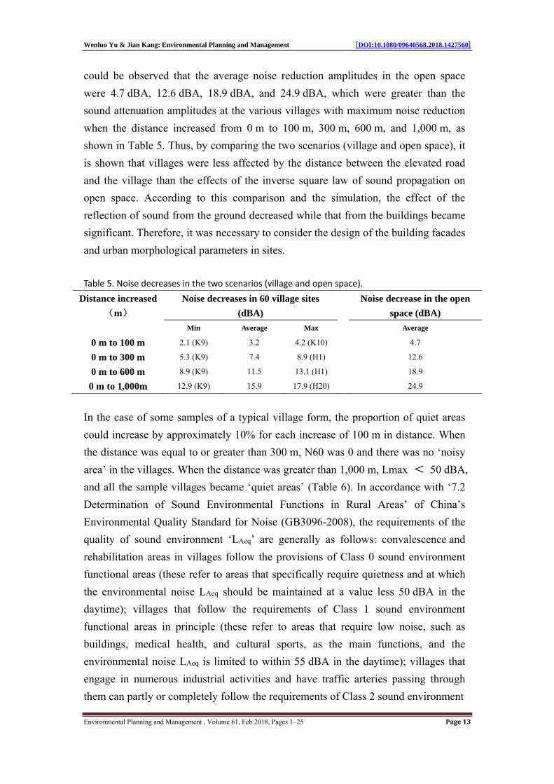
could be observed that the average noise reduction amplitudes in the open space
were 4.7 dBA, 12.6 dBA, 18.9 dBA, and 24.9 dBA, which were greater than the
sound attenuation amplitudes at the various villages with maximum noise reduction
when the distance increased from 0 m to 100 m, 300 m, 600 m, and 1,000 m, as
shown in Table 5. Thus, by comparing the two scenarios (village and open space), it
is shown that villages were less affected by the distance between the elevated road
and the village than the effects of the inverse square law of sound propagation on
open space. According to this comparison and the simulation, the effect of the
reflection of sound from the ground decreased while that from the buildings became
significant. Therefore, it was necessary to consider the design of the building facades
and urban morphological parameters in sites.
Table 5. Noise decreases in the two scenarios (village and open space).
Distance increased
(m)
Noise decreases in 60 village sites
(dBA)
Noise decrease in the open
space (dBA)
Min Average Max Average
0 m to 100 m 2.1 (K9) 3.2 4.2 (K10) 4.7
0 m to 300 m 5.3 (K9) 7.4 8.9 (H1) 12.6
0 m to 600 m 8.9 (K9) 11.5 13.1 (H1) 18.9
0 m to 1,000m 12.9 (K9) 15.9 17.9 (H20) 24.9
In the case of some samples of a typical village form, the proportion of quiet areas
could increase by approximately 10% for each increase of 100 m in distance. When
the distance was equal to or greater than 300 m, N60 was 0 and there was no ‘noisy
area’ in the villages. When the distance was greater than 1,000 m, Lmax < 50 dBA,
and all the sample villages became ‘quiet areas’ (Table 6). In accordance with ‘7.2
Determination of Sound Environmental Functions in Rural Areas’ of China’s
Environmental Quality Standard for Noise (GB3096-2008), the requirements of the
quality of sound environment ‘LAeq’ are generally as follows: convalescence and
rehabilitation areas in villages follow the provisions of Class 0 sound environment
functional areas (these refer to areas that specifically require quietness and at which
the environmental noise LAeq should be maintained at a value less 50 dBA in the
daytime); villages that follow the requirements of Class 1 sound environment
functional areas in principle (these refer to areas that require low noise, such as
buildings, medical health, and cultural sports, as the main functions, and the
environmental noise LAeq is limited to within 55 dBA in the daytime); villages that
engage in numerous industrial activities and have traffic arteries passing through
them can partly or completely follow the requirements of Class 2 sound environment

Wenluo Yu & Jian Kang: Environmental Planning and Management [DOI:10.1080/09640568.2018.1427560]
Environmental Planning and Management , Volume 61, Feb 2018, Pages 1–25 Page14
Table 6. Variances of the mean traffic noise level, noise area categories (%), and spatial noise
level indices Ln (dBA) among the 60 sites with horizontal distances between the site and
elevated roads of 0 m, 100 m, 300 m, 600 m, and 1,000 m.
Distance(m) Noise area categories (%) Spatial noise level indices, dBA
Quiet area Less Noisy Area Noisy Area Lmax L10 L50 L90
0 9.84 68.60 21.56 64.40 61.43 55.64 51.35
100 18.28 77.04 4.68 61.63 58.19 53.21 49.30
300 48.44 51.56 0.00 56.32 54.03 50.05 46.26
600 89.75 10.25 0.00 51.72 49.94 46.53 42.74
1,000 100.00 0.00 0.00 47.02 45.58 42.69 38.93
functional areas (these refer to areas that require maintenance of residential quietness,
that include country fair trade as the main function or single dwelling, commerce,
and industry, and in which the environmental noise LAeq is limited to within 60 dBA
in the daytime). Therefore, in these cases, the standard of Class 2 sound environment
functional areas would be satisfied when the distance between an elevated road and a
site is 300 m; that of Class 1 environment would be satisfied when the distance
between an elevated road and a site is 600 m, and Class 0 standard would be
satisfied when the distance between an elevated road and a site is more than 1,000 m.
For a distance of less than 300 m, this study compared and studied two types of
building facades, namely R3 (very smooth) and R0 (very rough or covered with
greenery). When the distance between the village and elevated road (10 m high) is
0 m, changing the building facades from R3 to R0 could cause a decrease in N60 of
the 60 samples by an average of 11.27%. When the distance is 100 m, N60 could
decrease by 3.17% on average. When the distance is greater than 100 m, the
influence is negligible. Therefore, the effective distance seems to be approximately
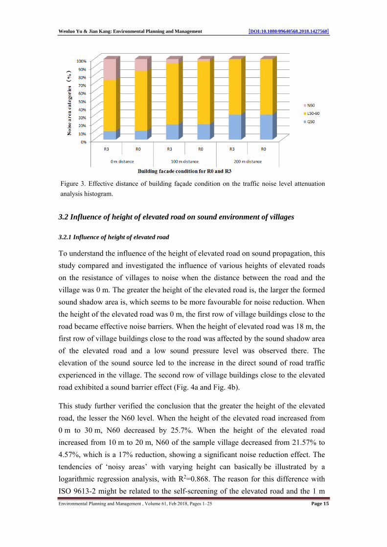
100 m (Fig. 3) for the noise reduction design of building facades. In terms of Q50,
when the distance is 0 m, 100 m, and greater than 100 m, Q50 could only increase by
0.52%, 0.27 %, and 0, which have negligible influence.
Wenluo Yu & Jian Kang: Environmental Planning and Management [DOI:10.1080/09640568.2018.1427560]
Environmental Planning and Management , Volume 61, Feb 2018, Pages 1–25 Page15
Figure 3. Effective distance of building façade condition on the traffic noise level attenuation
analysis histogram.
3.2 Influence of height of elevated road on sound environment of villages
3.2.1 Influence of height of elevated road
To understand the influence of the height of elevated road on sound propagation, this
study compared and investigated the influence of various heights of elevated roads
on the resistance of villages to noise when the distance between the road and the
village was 0 m. The greater the height of the elevated road is, the larger the formed
sound shadow area is, which seems to be more favourable for noise reduction. When
the height of the elevated road was 0 m, the first row of village buildings close to the
road became effective noise barriers. When the height of elevated road was 18 m, the
first row of village buildings close to the road was affected by the sound shadow area
of the elevated road and a low sound pressure level was observed there. The
elevation of the sound source led to the increase in the direct sound of road traffic
experienced in the village. The second row of village buildings close to the elevated
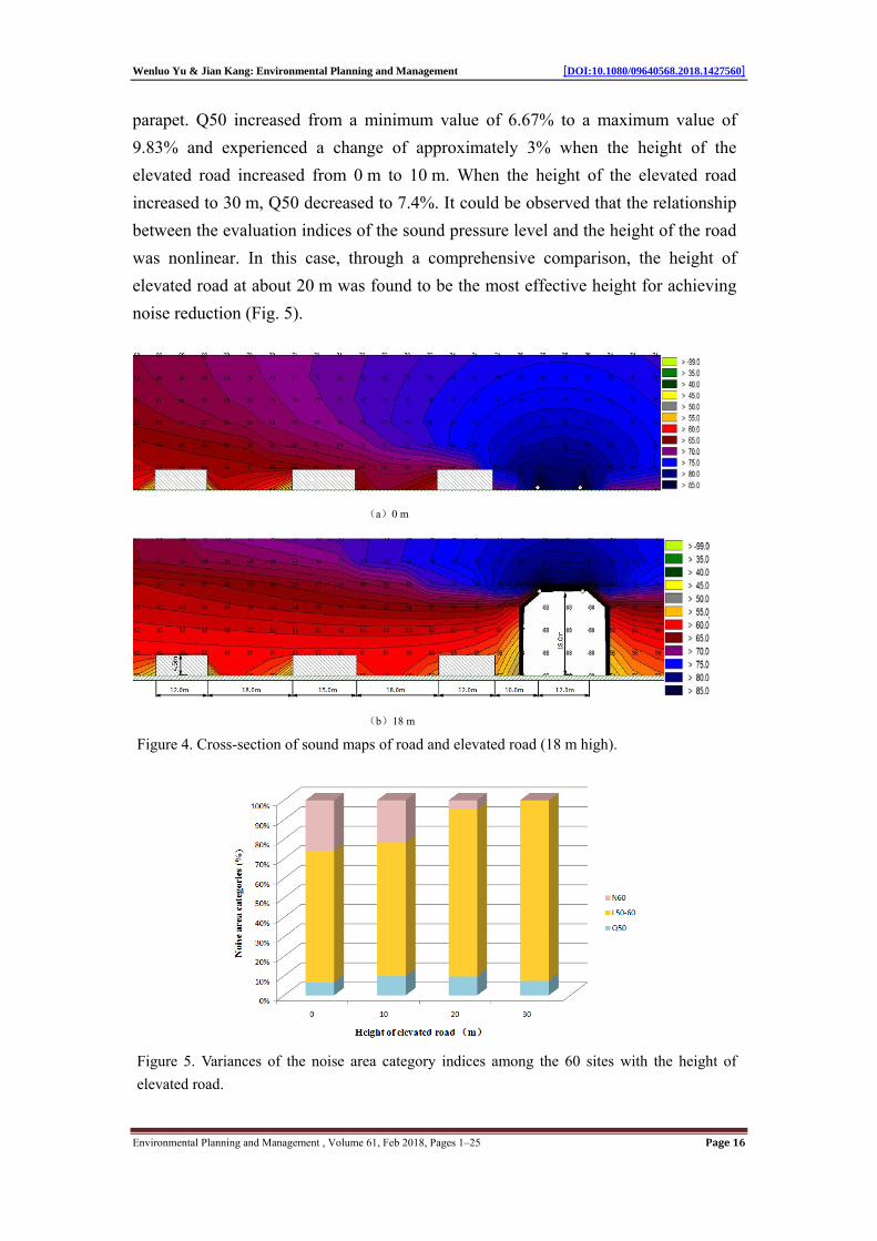
road exhibited a sound barrier effect (Fig. 4a and Fig. 4b).
This study further verified the conclusion that the greater the height of the elevated
road, the lesser the N60 level. When the height of the elevated road increased from
0 m to 30 m, N60 decreased by 25.7%. When the height of the elevated road
increased from 10 m to 20 m, N60 of the sample village decreased from 21.57% to
4.57%, which is a 17% reduction, showing a significant noise reduction effect. The
tendencies of ‘noisy areas’ with varying height can basically be illustrated by a
logarithmic regression analysis, with R2=0.868. The reason for this difference with
ISO 9613-2 might be related to the self-screening of the elevated road and the 1 m
Wenluo Yu & Jian Kang: Environmental Planning and Management [DOI:10.1080/09640568.2018.1427560]
Environmental Planning and Management , Volume 61, Feb 2018, Pages 1–25 Page16
parapet. Q50 increased from a minimum value of 6.67% to a maximum value of
9.83% and experienced a change of approximately 3% when the height of the
elevated road increased from 0 m to 10 m. When the height of the elevated road
increased to 30 m, Q50 decreased to 7.4%. It could be observed that the relationship
between the evaluation indices of the sound pressure level and the height of the road
was nonlinear. In this case, through a comprehensive comparison, the height of
elevated road at about 20 m was found to be the most effective height for achieving
noise reduction (Fig. 5).
(a)0 m
(b)18 m
Figure 4. Cross-section of sound maps of road and elevated road (18 m high).
Figure 5. Variances of the noise area category indices among the 60 sites with the height of
elevated road.
Wenluo Yu & Jian Kang: Environmental Planning and Management [DOI:10.1080/09640568.2018.1427560]
Environmental Planning and Management , Volume 61, Feb 2018, Pages 1–25 Page17
The above observation might have been made because the pavement of the elevated
road and the protection walls could be considered as sound barriers, which means
that the acoustic path difference due to the screening effect was the difference in the
value between the straight-line distance of the noise source of the elevated road to
the village and the indirect distance of the noise source of the road after bypassing
the sound barriers. The screening effect of the sound path difference was found to be
significant when the height of the road was approximately 20 m.
3.2.2 Influence of sound barrier of elevated road
The research area of the villages was a plane area. Therefore, in this study,
considering the maximum, median, and minimum area, and CAR and PD, three
typical villages H13 (50 hectares), K11 (32 hectares), and H20 (11 hectares) were
chosen from the 60 sites for analysis (Fig. 2).
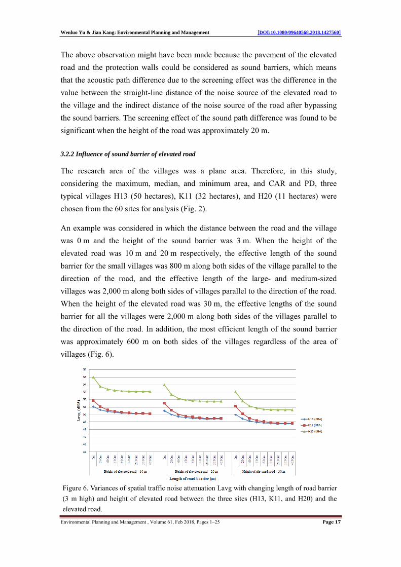
An example was considered in which the distance between the road and the village
was 0 m and the height of the sound barrier was 3 m. When the height of the
elevated road was 10 m and 20 m respectively, the effective length of the sound
barrier for the small villages was 800 m along both sides of the village parallel to the
direction of the road, and the effective length of the large- and medium-sized
villages was 2,000 m along both sides of villages parallel to the direction of the road.
When the height of the elevated road was 30 m, the effective lengths of the sound
barrier for all the villages were 2,000 m along both sides of the villages parallel to
the direction of the road. In addition, the most efficient length of the sound barrier
was approximately 600 m on both sides of the villages regardless of the area of
villages (Fig. 6).
Figure 6. Variances of spatial traffic noise attenuation Lavg with changing length of road barrier
(3 m high) and height of elevated road between the three sites (H13, K11, and H20) and the
elevated road.

Wenluo Yu & Jian Kang: Environmental Planning and Management [DOI:10.1080/09640568.2018.1427560]
Environmental Planning and Management , Volume 61, Feb 2018, Pages 1–25 Page18
The sound barrier of elevated roads is generally 1 m to 5 m. In order to eliminate the
influence of the length of the sound barrier (the length of barrier extended by
4,000 m along both sides of villages), this study considered an elevated road with a
height of 30 m as an example because the variances observed with this consideration
would be greater than those observed for the elevated road heights of 0 m, 10 m, and
20 m. Lavg was reduced by approximately 1.5 dBA on average among three typical
samples for each increase of 1 m in the height of the sound barrier. However, the
increase in the height of the sound barrier did not show a simple linear relationship
with the attenuation of Lavg. It was observed that the influence of the increase in the
height of the road on the sound environment of large- and medium-sized villages
was slightly greater than that on small villages. The noise experienced in large- and
medium-sized villages was reduced by 2 dBA, which was more than that in small
villages, on average (Fig. 7).
Figure 7. Variances of the spatial traffic noise attenuation Lavg with changing height of road
barrier between the three sites (H13, K11, and H20) and the 30 m high elevated road.
3.3 Influence of morphological parameters of villages
3.3.1 Relationship between sound evaluation indices and morphological parameters
Considering that the two noise area categories (area ratio N60 of noisy areas and
area ratio of quiet areas Q50) of villages in severely cold areas were potentially
correlated with the six morphological parameters, SPSS 21.0 was used in this study
to compute the Spearman correlation (the results of the Pearson correlation
coefficients were very close to those of the Spearman correlation analysis; however,
because not all the variables satisfy the normal distribution, it is not appropriate to
use the Pearson correlation analysis) (Du, 2010). When the distance was 0 m, N60

Wenluo Yu & Jian Kang: Environmental Planning and Management [DOI:10.1080/09640568.2018.1427560]
Environmental Planning and Management , Volume 61, Feb 2018, Pages 1–25 Page19
was significantly correlated with LSI_B, PD, and RLF (p < 0.01) as well as with
CAR, RIF, and LSI_R (p < 0.05). When the distance was more than 100 m, N60 was
0. In addition, Q50 was significantly correlated with LSI_B and LSI_R (p < 0.01)
for distances of 0 m, 100 m, and 300 m, as well as with CAR when the distance was
0 m and 100 m (p < 0.05) (Table 7).
Table 7. Spearman’s rho correlations between the noise area category indices Q50 in the villages
and the urban morphological parameters (2-tailed). Significant correlations are marked with *
(p < 0.05) and ** (p < 0.01).
Distance
(m)
Indices
(%) Urban morphological parameters
CAR LSI_B PD RLF RIF LSI_R
0 N60 .300* ‐.416** .346** .358** .257* ‐.297*
0 Q50 ‐.287* .684** ‐.228 ‐.106 ‐.018 .692**
100 Q50 ‐.256* .640** ‐.213 ‐.054 .045 .662**
300 Q50 ‐.099 .403** ‐.097 ‐.107 ‐.046 .402**
** p < 0.01 (2‐tailed)
* p < 0.05 (2‐tailed)
Furthermore, a regression analysis was conducted on the significantly correlated
parameters (p < 0.01). Because the regression analysis results (R2) of N60
(N60-LSI_B inverse regression analysis R2 = 0.269; N60-PD cubic regression
analysis R2 = 0.164; N60-RLF cubic regression analysis R2 = 0.096) were less than
0.3 and the regression effect was poor, a stepwise multiple regression analysis was
performed after considering the other parameters, HWR_V (0.40), LSI_B (−0.35),
and RLF (0.26), that caused a change in N60. The results showed that R2 = 0.436 <
0.5, and the regression effect was still poor.
In this study, a regression analysis was conducted on Q50-LSI_B and Q50-LSI_R,
and the representative distances of 0 m and 100 m were considered as examples.
When the distance was 0 m, two groups of parameters could be related linearly (Fig.
8).
Q50 could be increased by approximately 68% with the increase in LSI_B from
5.824 to 24.103, as can be seen in Fig. 8a. This was probably because increasing the
complexity of the buildings in villages could improve the sound barrier effect of
those buildings. On comparing the village samples with various LSI_B values, it was
found that large villages with multiform buildings or a mixed layout showed a strong
anti-noise performance. As R2 < 0.5, a multiple stepwise regression analysis was
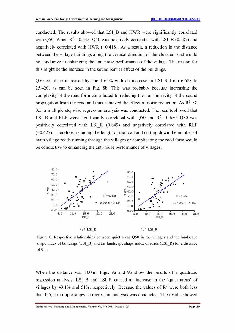
Wenluo Yu & Jian Kang: Environmental Planning and Management [DOI:10.1080/09640568.2018.1427560]
Environmental Planning and Management , Volume 61, Feb 2018, Pages 1–25 Page20
conducted. The results showed that LSI_B and HWR were significantly correlated
with Q50. When R2 = 0.645, Q50 was positively correlated with LSI_B (0.587) and
negatively correlated with HWR (−0.418). As a result, a reduction in the distance
between the village buildings along the vertical direction of the elevated road would
be conducive to enhancing the anti-noise performance of the village. The reason for
this might be the increase in the sound barrier effect of the buildings.
Q50 could be increased by about 65% with an increase in LSI_R from 6.688 to
25.420, as can be seen in Fig. 8b. This was probably because increasing the
complexity of the road form contributed to reducing the transmissivity of the sound
propagation from the road and thus achieved the effect of noise reduction. As R2 <
0.5, a multiple stepwise regression analysis was conducted. The results showed that
LSI_R and RLF were significantly correlated with Q50 and R2 = 0.650. Q50 was
positively correlated with LSI_R (0.849) and negatively correlated with RLF
(−0.427). Therefore, reducing the length of the road and cutting down the number of
main village roads running through the villages or complicating the road form would
be conductive to enhancing the anti-noise performance of villages.
(a)LSI_B (b)LSI_R
Figure 8. Respective relationships between quiet areas Q50 in the villages and the landscape
shape index of buildings (LSI_B) and the landscape shape index of roads (LSI_R) for a distance
of 0 m.
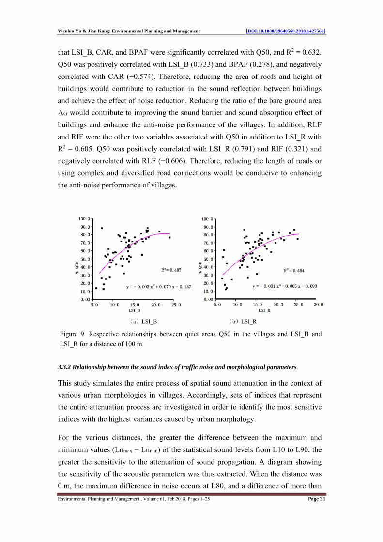
When the distance was 100 m, Figs. 9a and 9b show the results of a quadratic
regression analysis: LSI_B and LSI_R caused an increase in the ‘quiet areas’ of
villages by 49.1% and 51%, respectively. Because the values of R2 were both less
than 0.5, a multiple stepwise regression analysis was conducted. The results showed
Wenluo Yu & Jian Kang: Environmental Planning and Management [DOI:10.1080/09640568.2018.1427560]
Environmental Planning and Management , Volume 61, Feb 2018, Pages 1–25 Page21
that LSI_B, CAR, and BPAF were significantly correlated with Q50, and R2 = 0.632.
Q50 was positively correlated with LSI_B (0.733) and BPAF (0.278), and negatively
correlated with CAR (−0.574). Therefore, reducing the area of roofs and height of
buildings would contribute to reduction in the sound reflection between buildings
and achieve the effect of noise reduction. Reducing the ratio of the bare ground area
AG would contribute to improving the sound barrier and sound absorption effect of
buildings and enhance the anti-noise performance of the villages. In addition, RLF
and RIF were the other two variables associated with Q50 in addition to LSI_R with
R2 = 0.605. Q50 was positively correlated with LSI_R (0.791) and RIF (0.321) and
negatively correlated with RLF (−0.606). Therefore, reducing the length of roads or
using complex and diversified road connections would be conducive to enhancing
the anti-noise performance of villages.
(a)LSI_B (b)LSI_R
Figure 9. Respective relationships between quiet areas Q50 in the villages and LSI_B and
LSI_R for a distance of 100 m.
3.3.2 Relationship between the sound index of traffic noise and morphological parameters
This study simulates the entire process of spatial sound attenuation in the context of
various urban morphologies in villages. Accordingly, sets of indices that represent
the entire attenuation process are investigated in order to identify the most sensitive
indices with the highest variances caused by urban morphology.
For the various distances, the greater the difference between the maximum and
minimum values (Lnmax − Lnmin) of the statistical sound levels from L10 to L90, the
greater the sensitivity to the attenuation of sound propagation. A diagram showing
the sensitivity of the acoustic parameters was thus extracted. When the distance was
0 m, the maximum difference in noise occurs at L80, and a difference of more than

Wenluo Yu & Jian Kang: Environmental Planning and Management [DOI:10.1080/09640568.2018.1427560]
Environmental Planning and Management , Volume 61, Feb 2018, Pages 1–25 Page22
10 dBA was observed with the mean of the difference between the maximum and
minimum values. When the distance was 100 m and 300 m, the value of
Lnmax − Lnmin of L10 was the largest, varying by more than 8 dBA and 6 dBA,
respectively, with the mean of the difference between the maximum and minimum
values (Fig. 10). Therefore, the selection of sound indices of sensitivity is as follows:
L80 for 0 m and L10 for 100 m to 300 m.
Figure 10. Statistical sound level indices of the 60 sites with the mean difference between the
maximum and minimum values shown for each index. The various coloured lines represent
distances of 0 m, 100 m, and 300 m between the site and the elevated road.
This study computed the Spearman correlation between the indices of the sound
pressure levels and morphological parameters. For the various distances, LSI_B and
LSI_R were significantly correlated with the indices of the statistical sound levels
(p < 0.01). RLF and RIF were not correlated with any other acoustic indices (Table
8). Similarly, the distances of 0 m and 100 m were considered as examples. This
study further conducted a regression analysis on the related parameters. When the
distance was 0 m, L80-LSI_B and L80-LSI_R could be predicted using an inverse
function and a quadratic relationship, respectively (Fig. 10).
Table 8. Correlations between spatial traffic noise levels in the villages and urban morphological
parameters (2‐tailed). Significant correlations are marked with * (p < 0.05) and ** (p < 0.01).
Distance
(m)
Indices
(dBA) Urban morphological parameters
CAR LSI_B PD RLF RIF LSI_R
0 L80 .289* -.686** .249 .117 .012 -.690**
100 L10 .259* -.470** .284* .133 .036 -.424**
300 L10 021 -.481** .029 .056 .015 -.490**
** p < 0.01 (2-tailed)
* p < 0.05 (2-tailed)

Wenluo Yu & Jian Kang: Environmental Planning and Management [DOI:10.1080/09640568.2018.1427560]
Environmental Planning and Management , Volume 61, Feb 2018, Pages 1–25 Page23
When LSI_B ≤ 12, L80 sharply decreased by 6.2 dBA with the increase in LSI_B,
and when LSI_B > 12, L80 gradually decreased by 3 dBA (Fig. 11a). This was
probably because increasing the complexity of building form in the villages could
lead to more sound reflection between buildings and thus reduce the sound barrier
effect of the buildings. L80 could decrease by approximately 8.4 dBA with the
increase in LSI_R (Fig. 11b). This was probably because increasing the complexity
of the road form in rural residential areas was conducive to reducing the sound
propagation through the streets along the roads and achieving the effect of noise
reduction.
When the distance was 100 m, there was no specific change rule between the
variables of the scatter diagram of L10-LSI_B and L10-LSI_R. In various instances
in the curve regression, R2 was less than 0.2. In addition, R2 was less than 0.4 in the
multiple regression equations. Therefore, it could be neglected.
(a)LSI_B (b)LSI_R
Figure 11. Respective relationships between the spatial noise level indices L80 in the villages
and LSI_B and LSI_R for a distance of 0 m.
4. Conclusions
The problem of traffic noise from elevated roads is extremely serious in rural
villages. In this study, the methods of improving the anti-noise properties of villages
through a systematic design were investigated, and the following conclusions were
drawn:
1. Increasing the distance between villages and elevated roads could effectively
reduce the influence of traffic noise on villages; however, there would be significant
differences in the noise reduction effect for villages of different forms. Thus, it was
Wenluo Yu & Jian Kang: Environmental Planning and Management [DOI:10.1080/09640568.2018.1427560]
Environmental Planning and Management , Volume 61, Feb 2018, Pages 1–25 Page24
necessary to consider the design of building facades and the noise reduction effect
caused by the village forms. For samples of a typical village form, the proportion of
‘quiet areas’ could increase by approximately 10% for each increase of 100 m in the
distance between the elevated road and the village. When the distance was 300 m,
the proportion of noisy areas was 0, which would satisfy the standard of Class 2
sound environment functional areas according to the ‘Environmental Quality
Standard for Noise’ (GB3096-2008). When the distance was 600 m, the Class 1
living standard could be satisfied. The Class 0 standard could be satisfied when the
distance between the elevated road and the village was more than 1,000 m. The
effective distance in the design for the noise reduction of building facades was
approximately 100 m. When the distance was more than 100 m, there would be no
requirement for considering noise reduction measure such as changing the materials
of the building facades or designing vertical greenery systems.
2. The sound shadow area formed by a higher elevation road would be more
conducive to noise reduction. When the height of the elevated road increased from
0 m to 30 m, N60 decreased by 25.7%. The influence of the height of elevated road
on the occurrence of ‘noisy areas’ was more significant than that of Q50. In
comparison, the sound barrier effect of the sound path difference caused by the
elevated road with a height at about 20 m was the most significant. When the height
of the elevated road was 10 m to 30 m, the sound barrier was 3 m high. Regardless
of the village area, the most economical and efficient length of the sound barrier was
approximately 600 m along both sides of the village parallel to the road. In addition,
the influence of the length of the sound barrier was neglected. For each increase of
1 m in the height of the sound barrier, Lavg of the three typical samples reduced by
approximately 1.5 dBA, on average. The sound environments of large- and
medium-sized villages were affected by the height of the sound barrier to some
extent, and a noise reduction of approximately 0.2 dBA more than Lavg in small
villages was observed.
3. Decreasing the spatial traffic noise levels of an elevated road and enlarging the
quiet areas in villages by controlling the urban morphological parameters of villages
are efficient measures of noise reduction. As shown in the single element and
multiple regression analyses, there are a series of significant relationships between
the spatial traffic noise levels and the urban morphological parameters, with R2 >
0.5. In addition, the morphological parameters affecting the noise attenuation were
different for the various distances. When the distance was 0 m, the ‘quiet areas’ had
a positive relationship with the indices of the buildings, LSI_B and LSI_R, and a
Wenluo Yu & Jian Kang: Environmental Planning and Management [DOI:10.1080/09640568.2018.1427560]
Environmental Planning and Management , Volume 61, Feb 2018, Pages 1–25 Page25
negative relationship with HWR and RLF. When the distance was 100 m, the ‘quiet
areas’ are positively associated with LSI_B, BPAF, LSI_R, and RIF and negatively
associated with CAR and RLF. In terms of the spatial noise level indices, L80 has a
negative relationship with LSI_B and LSI_R. In addition, the ‘noisy areas’ did not
show an obvious relationship with the morphological parameters of the villages
when the distance was 0 m, and L10 did not show an obvious relationship with
LSI_B or LSI_R when the distance was 100 m.
This study examines the methods of reducing elevated-road traffic-noise levels in
rural residential areas. Based on previous research results, it systematically revealed
whether and how relative locations and morphological parameters influence the
spatial noise level attenuation of elevated roads. In addition, the effects of noise
barriers and building facades in villages on noise attenuation were also examined.
Overall, by filling the gaps in previous studies, this study is expected to provide
guidance and data for village and elevated road designers and local authorities,
particularly relating to the village planning system in cold areas in China. However,
the results cannot be applied to other climates and geographical environments, such
as rural villages in severely hot areas (for a larger building density, a larger number
of reflections will be set up) and mountainous regions, whose terrain has a great
influence on the noise prediction results. The influence of topography on the acoustic
environment should be considered in actual elevated composite road projects.
Mountainous regions, being huge acoustic barriers, require consideration of
more influencing factors owing to the complexity of the acoustic environment (form,
layout, scale, and the sound absorption coefficient of the mountain). Research
methods are available for reference on similar issues in other climates and
geographical environment.

Wenluo Yu & Jian Kang: Environmental Planning and Management [DOI:10.1080/09640568.2018.1427560]
Environmental Planning and Management , Volume 61, Feb 2018, Pages 1–25 Page26
References [1] Avsar, Y., and M. T. Gonullu. 2005. “Determination of Safe Distance Between
Roadway and School Buildings to Get Acceptable School Outdoor Noise Level by Using Noise Barriers.” Building and Environment 40 (9): 1255–1260.
[2] Burian, S. J., W. S. Han, and M. J. Brown. 2005. Morphological Analyses Using 3D Building Databases: Oklahoma City, Oklahoma. LA-UR-05-1821. Los Alamos, NM: Los Alamos National Laboratory.
[3] Chen, X. Y., and H. B. Xiong. 2013. “Prediction and Control Techniques Research on Environmental Effect of Noise from Elevated Roads.” MSc Thesis, Harbin Institute of Technology.
[4] Chen, Y. L., Q. Sun, W. Wei, K. B. Liu, and C. M. Liu. 2007. “Investigation on Traffic Noise Pollution Caused by Overhead Road.” Environmental Health : A Global Access Science Source 24 (10): 795–797.
[5] DataKustik GmbH. 2006. Cadna/A for Windows: User Manual. Munich: Kustik. [6] Du, Z. M. 2010. Sample Survey and the Application of SPSS Software. Beijing:
Electronics Industry Publishing. [7] Fritschi L., A. L. Brown, R. Kim, D. H. Schwela, and S. Kephalopoulos, eds.2011.
Burden of Disease from Environmental Noise: Quantification of Healthy Life Years Lost in Europe. Geneva: World Health Organisation, Regional Office for Europe. http://www.euro.who.int/__data/assets/pdf_file/0008/136466/e94888.pdf.
[8] GB 3096-2008, 2008. Environmental Quality Standard for Noise. Beijing: State Environmental Protection Administration of China.
[9] Hao, Y., and J. Kang. 2014. “Influence of Mesoscale Urban Morphology on the Spatial Noise Attenuation of Flyover Aircrafts.” Applied Acoustics 84 (84): 73–82.
[10] Hao, Y., J. Kang, D. Krijnders, and H. Wörtche, 2015. “On the Relationship Between Traffic Noise Resistance and Urban Morphology in Low-Density Residential Areas.” Acustica/acta Acustica-European Journal of Acoustics 101 (3): 510–519 (10).
[11] He, P., and H. R. Zhang. 2009. “Study on Factor Analysis and Selection of Common Landscape Metrics.” Forest Research 22: 470–474.
[12] He, Y., and J. Kang. 2014. “Differences Between Rural and Urban Sound Environment in Northeast of China.” MSc Thesis, Harbin Institute of Technology, 10–19.
[13] Heilongjiang Provincial Bureau of Statistics. 2014. Heilongjiang Statistical Yearbook. Beijing: China Statistics Press.
[14] ISO 9613-2, 1996, Acoustics – Attenuation of Sound During Propagation Outdoors – Part 2: General Method of Calculation. Geneva: International Standards Organization.
[15] JTG D20-2006. 2006. Design Specification for Highway Alignment. Beijing: China’s Ministry of Transport.
[16] Kang, J. 2007. Urban Sound Environment. London: Taylor & Francis. [17] Kim, M. J., and H. G. Kim. 2007. “Field Measurements of Façade Sound
Insulation in Residential Buildings with Balcony Windows.” Building and
Wenluo Yu & Jian Kang: Environmental Planning and Management [DOI:10.1080/09640568.2018.1427560]
Environmental Planning and Management , Volume 61, Feb 2018, Pages 1–25 Page27
Environment 42 (2): 1026–1035. [18] Ko, J. H., S. I. Chang, M. Kim, J. B. Holt, and J. C. Seong. 2011. “Transportation
Noise and Exposed Population of an Urban Area in the Republic of Korea.” Environment International 37 (2): 328–334.
[19] Lam, K. C., W. Ma, P. K. Chan, W. C. Hui, K. L. Chung, Y. T. Chung, C. Y. Wong, and H. Lin. 2013. “Relationship Between Road Traffic Noisescape and Urban Form in Hong Kong.” Environmental Monitoring and Assessment 185 (12): 9683–9695.
[20] Li H., Z. D. Li, and M. Li. 2012. “Application of Cadna/A Software in Prediction and Assessment of Expressway Noise.” Environmental Science and Management 37 (1): 168–172.
[21] Li, X., and S. W. Yang. 2013. “Key Technology for Expressway Land Intensive Economical Use and Comprehensive Evaluation on Its Effect.” PhD Thesis, Chang’ an University.
[22] Li, G. X., J. Y., Zhu, and Y. M. Sun. 2007. “Feasibility Study on Applying Rubber Road Pavement on Urban Viaducts to Reduce Vibration or Noise.” Technology of Highway and Transport 5: 127–129.
[23] Liu, L. Q. 2008. “The Discussion of a New Design Idea: Bridges Instead of Roads and Bridges Instead of Tunnels.” Highway Engineering 33 (2): 114–117.
[24] Liu, J., J. Kang, H. Behm, and T. Luo. 2014. “Effects of Landscape on Soundscape Perception: Soundwalks in City Parks.” Landscape and Urban Planning 123 (1): 30–40.
[25] Ma, X., and S. Li. 2009. “Optimization Design of L-Shaped Road Noise Barrier and Cost-Effectiveness Analysis.” In Proceedings for the 2009 IEEE Intelligent Vehicles Symposium, 998–993. New York: IEEE. doi:10.1109/IVS.2009.5164415
[26] Mei, L., and J. Kang. 2014. “Research on Courtyard Acoustic Environment of Rural Housing in Severe Cold Area of Northeast China.” MSc Thesis, Harbin Institute of Technology.
[27] Mei, L., J. Kang, and M. Huang. 2016. “Acoustic Comfort Evaluation and its Influencing Factors in Courtyards of Cold Rural Regions.” Building Science 32 (2): 43–47.
[28] Meng, X. Q., and J. Kang. 2014. “The Interact Between the Main Road Traffic Noise and the Village Planning of Northeast.” MSc Thesis, Harbin Institute of Technology.
[29] Murthy, V. K., A. K. Majumder, S. N. Khanal, and D. P. Subedi. 2010. “Assessment of Traffic Noise Pollution in Banepa: A Semi Urban Town of Nepal.” Kathmandu University Journal of Science Engineering and Technology 3 (2): 12–20.
[30] Oke, T. R. 1988. “Street Design and Urban Canopy Layer Climate.” Energy and Buildings 11 (1-3):103–113.
[31] Rey Gozalo, G., J. M. BarrigónMorillas, and V. Gómez Escobar. 2012. “Analysis of Noise Exposure in Two Small Towns.” Acta Acustica United with Acustica 98 (6): 884–893.
[32] Rey Gozalo, G., J. M. BarrigónMorillas, V. Gómez Escobar, R. Vílchez-Gómez, J.
Wenluo Yu & Jian Kang: Environmental Planning and Management [DOI:10.1080/09640568.2018.1427560]
Environmental Planning and Management , Volume 61, Feb 2018, Pages 1–25 Page28
A. Méndez Sierra, and F. J. Carmona del Río, et al., 2013. “Study of the Categorisation Method Using Long-Term Measurements.” Archives of Acoustics 38 (3): 397–405.
[33] Salomons, E. M., and M. B. Pont. 2012. “Urban Traffic Noise and the Relation to Urban Density, Form, and Traffic Elasticity.” Landscape and Urban Planning 108 (1): 2–16.
[34] Shao, T., H. Jin, and L. H. Zhao. 2016. “The Existing Situation and Improving Strategies for Rural Housings in the Northeast Severe Cold Regions.” China Sciencepaper 11 (1): 12–16.
[35] Sobotova, L., J. Jurkovicova, Z. Stefanikova, L. Sevcikova, and L. Aghova. 2010. “Community Response to Environmental Noise and the Impact on Cardiovascular Risk Score.” The Science of the Total Environment 408 (6): 1264–1270.
[36] Stephen, M. 2004. Street and Patterns. London: Taylor & Francis. [37] Sun, H. T., P. J. Liu, and H. W. Wang. 2010. “The Noise Prediction of Urban
Elevated Road Based on Cadna /A.” South China Normal University (Natural Science Edition) 1: 58–61.
[38] Voogt, J. A., and T. R. Oke. 1997. “Complete Urban Surface Temperatures.” Applied Meteorology 36 (9): 1117–1132.
[39] Wang, X. J. 2014. “Current Situation and Development Trend of Rural Building.” Nong Min Zhi Fu Zhi You 11: 154–154.
[40] Wang, Y. P., and L. Gai. 2012. “Study on the Distribution of Sound Field in Vertical Plane of Traffic Noise for City Elevated Complex Road.” Noise and Vibration Control 5: 136–140.
[41] Wang, B., and J. Kang. 2011. “Effects of Urban Morphology on the Traffic Noise Distribution Through Noise Mapping: A Comparative Study Between UK and China.” Applied Acoustics 72 (8): 556–568.
[42] Wong, N. H., A. Y. K. Tan, P. Y. Tan, K. Chiang, and N. C. Wong. 2010. “Acoustics Evaluation of Vertical Greenery Systems for Building Walls.” Building and Environment 45 (2): 411–420.
[43] Wu, C. S. 1998. “Properly Replace Railway by Bridge and Economize on Good Farmland: A Great Contribution for People.” Railway Engineering Society 15 (1): 35–38.
[44] Xi, O., Y. M. Zeng, Y. Shen, X. W. Wei, Y. Q. Wang, and M. M. Yuan. 2015. “Discussion on Domestic Rural Noise Pollution Status and its Control Measures.” Noise and Vibration Control 35 (2): 131–136.
[45] Yang, Y. M. 2016. “Effects of Elevated Road on Noise Environment of Neighbouring Street Residential Building.” Environmental Science and Management 41 (9): 60–64.
[46] Yang, H. S., J. Kang, and M. S. Choi. 2012. “Acoustic Effects of Green Roof Systems on a Low-Profiled Structure at Street Level.” Building and Environment 50 (4): 44–55.
[47] Yari, A., B. Dezhdar, A. Koohpaei, A. Ebrahimi, A. Mashkoori, M. J. Mohammadi, and S. A. Jang. 2016. “Evaluation of Traffic Noise Pollution and Control Solutions Offering: A Case Study in Qom, Iran.” Kerman University of

Wenluo Yu & Jian Kang: Environmental Planning and Management [DOI:10.1080/09640568.2018.1427560]
Environmental Planning and Management , Volume 61, Feb 2018, Pages 1–25 Page29
Medical Sciences, 23 (4): 600–607. [48] Ye, J., G. H. Xia, and B. Hu. 2016. “Space Distribution and Control Measures of
Elevated Road Traffic Noise of Wenling City.” Environmental Science and Management, 41 (6): 133–136.
[49] Yu, W. Z. 2008. “Noise Reduction Effect of Sound Barrier of Elevated Road.” Chinese Journal of Environmental Engineering 2 (6): 844–847.
[50] Yu, X. F., and Y. Gao. 2013. “On Sensitivity Analysis of Various Acoustic Barriers on Noises at Viaducts.” Shanxi Architecture 39 (20): 194–196.
[51] Yu, W. L., and J. Kang. 2016. “Analysis of the Integrated Effects of Village Form on Traffic Noise Resistance in Severe Cold Region.” Urbanism and Architecture 28: 109–113.
[52] Yu, W. L., and J. Kang. 2017. “Relationship Between Traffic Noise Resistance and Village Form in China.” Landscape and Urban Planning 163: 44–55.
[53] Zhang, L. J. 2014. “Study on Analysis and Control Technology of Noise Situation Surrounding Viaduct at Changzhou.” MSc Thesis, Harbin Institute of Technology.
[54] Zhang, L., and Y. Rao. 2012. “Research on Simulation of Acoustics Environment and Noise Cancelling Design Strategy of the Residential District Along the Road in Hefei.” MSc Thesis, Hefei University of Technology.
[55] Zhang, X. 2004. “The Characteristics of Elevated Road Traffic Noise and Noise Control.” Paper presented at a conference on Green Buildings and Buildings, Southeast University, Nanjing, China, October 15–17.
[56] Zhang, T. Y., and Q. Yin. 2014. “The Research of Optimization Strategy of the Wind Environment of the Residential Buildings and the Courtyard in the Cold Region of the Northeast of China.” MSc Thesis, Harbin Institute of Technology.