Resistance of rectangular conductors - G3RBJ |...

Payne : The ac Resistance of Rectangular Conductors

1

THE AC RESISTANCE OF RECTANGULAR CONDUCTORS

A simple equation is given here for the ac resistance of rectangular conductors. This is

shown to give good agreement with independent measurements for all shapes of

rectangular conductor from very thin strip to square section.

1. INTRODUCTION

A rigorous treatment of the ac resistance of conductors with a rectangular section leads to formidable

mathematical difficulties, and many authors have tried to overcome these problems over the past 100 years

but without success. Given that there is no useful theory the curves by Haefner (ref 1) are widely published,

and these are shown below. His paper was written in 1937 and so it is surprising that no analytical analysis

has replaced it.

The theoretical approach here is to simplify the problem by assuming that current diffuses from the four

faces independently. This along with experimentally derived factors give a simple equation which is shown

to be surprisingly accurate for all shapes of rectangular conductor from thin strip to square cross-section.

2. HAEFNER’S MEASUREMENTS

2.1. Published graphs

Haefner measured the ac resistance of five copper conductors having width to thickness (w/t) ratios of 1, 2,

5, 10, and 2400, and over a frequency range from 0 to 8 KHz. Each conductor was around 60 ft in length,

folded back on itself with a spacing of about 2ft which he had checked would have negligible proximity

effect. In addition to his own measurements he also used measurements published by other experimenters.

A summary of his findings is given in the graph below, extracted from Terman (ref 2) :

Figure 2.1 Haefner’s results


2

The other experimenters had used different sized conductors to his and measured them at different

frequencies, and so to combine all these measurements he used the principle of ‘similitude’. This had

previously been enunciated by Dwight who found that if measurements of resistance were plotted against

the parameter p = [8π f /(109 Rdc)]

0.5, the plot can be used to predict the resistance under different conditions

to the measurements. For instance measurements made on large conductors at low frequencies are valid for

small conductors at high frequencies and vice versa. The curve for the round wire above provides a good

example of the usefulness of this approach since only one curve is needed for round wire of any diameter,

and at any frequency.

Haefner also expresses p as

p = [8π f A/ ρa ]0.5

2.1.1

In this case the area is in cms2 and the specific resistance ρa is in absohms/cm

3, which for copper ρa =1724.

This is not in a convenient form today because the resistance R is expressed in absohms. It is easier and

more informative to re-write the parameter as :

p = A 0.5

/ (1.26 δ) 2.1.2

where A is the cross-sectional area in mm2

δ is the skin depth = [ρ/(πfµ)]0.5

in mm

It can now be seen that the parameter p is the ratio of two lengths, one related to the size of the conductor

and the other the skin depth. Notice that this equation includes the permeability, which in Haefner’s

equation is assumed to be unity.

The above curves are a combination of experimental and calculated results, with the dotted portions

representing the extrapolation of low frequency measurements to join some theoretical results by Cockroft

(ref 3) at high frequencies. These extrapolations could therefore be valid if Cockroft’s high frequency

theory was correct but this is unproven because he was unable to find any published measurements against

which to verify his theory. These extrapolations must be treated therefore with some caution.

The above graph is widely reproduced but not always with the dotted lines, so that it is then not clear that

much of the graph consists of extrapolations.

Note :

In some versions of the above graph the horizontal axis p is given as (f/Ro)0.5

, where f is in Hz and Ro is in

µΩ/m (for instance the Copper Association ref 4). Multiplying this factor by 1.58 gives p as defined by

Equation 2.1.1 or 2.1.2.

Alternatively p has been given in terms of (f/Ro 1000m)0.5

, where f is in Hz and Ro 1000m is the dc resistance of

1000 meter length. Dividing this equation by 20 gives p as defined by Equation 2.1.1 or 2.1.2.

2.2. Extrapolation of Haefner’s measurements

A large proportion of Haefner’s graph consists of extrapolations from measurements, and so it raises the

question as to how accurate these might be. Also further extrapolation may be necessary if his curves are to

used beyond the values given.

An insight into this extrapolation can be gained by considering the round conductor, because the resistance

of this is well understood and predictable. At very high frequencies the conducting area is a narrow band

around the circumference of the wire and of thickness equal to the skin depth δ. The conducting area is

therefore A= (π d δ). The ratio of the high frequency resistance to the low frequency resistance is thus equal

to the ratio of the conducting areas :

Rac/Rdc ≈ (πd2/4)/ (π d δ) = 0.25 d/δ 2.2.1

From Equation 2.1.2, p = d/ (1.48 δ). Thus the limiting value of the slope of Haefner’s round wire curve at

high frequencies should be by this calculation :

Limiting value of [(Rac/Rdc) / p] = 0.36 2.2.2


3

And indeed this is what it is. However we can anticipate that the curves for the rectangular conductors will

also have this same limiting slope. This will apply as long as the frequency is sufficiently high that ‘the

radius of curvature of the conductor surface is everywhere appreciably greater than the skin depth and does

not vary too rapidly around the periphery’ (Terman ref 2, page 34). Of course this can never be true for a

rectangular conductor with perfectly sharp corners, but a practical conductor will have rounded corners.

Indeed Haefner notes that the samples he measured had ‘… edges slightly rounded, as is the case in the

commercial production of such strip conductors’.

Indications of this limiting slope can be seen in Figure 2.1 where the slopes of the curves for w/t = 4 and

w/t = 8 are increasing towards that of the round conductor as p increases. The curve for w/t =16 also shows

this trend. The curve for w/t = 24 does not, but beyond p=5 it is linearly extrapolated and this may be

wrong. Indeed the theory presented here shows an increasing slope at this value of p (see comparisons

Section 6).

Cockroft’s analysis gives limiting slopes depending on the factor p. For instance for the square cross-

section he gives this as 0.418p for p>3.2, whereas Haefner’s curve is 0.37 p. For w/t = 8 Cockroft gives

0.29, whereas Haefner’s curve is 0.34 at p =10, and the slope is clearly still increasing (see ref 1 for

Cockroft’s data). So it would seem that Cockroft’s limiting values do not agree with experiment.

3. KEY FACTORS

3.1. Introduction

There are two key factors which determine the ac resistance of rectangular conductors : a) the diffusion of

current into the conductor from the four surfaces, and b) current crowding whereby the current concentrates

at the corners and edges. These are considered below.

3.2. Diffusion of current

It is well known that at high frequencies the current in a conductor tends to concentrate in a thin layer

around its surface. For instance a conductor with a circular cross-section carries current in only a thin layer

around its circumference, so that its high frequency resistance is the same as a hollow tube with a thickness

equal to the skin depth. At all points around this circumference this current has the same density.

Skin effect arises because current diffuses into a conductor from the outside. The amplitude of this current

is greatest at the surface and decreases exponentially with depth (ref 5):

Figure 3.2.1 Current density at depth

This exponentially decaying current has the same area as that of a current uniformly distributed down to

depth of δ, and zero at greater depths and this leads to the definition of skin depth :

Skin depth δ = [ρ/(πfµ)]0.5

3.2.1


4

There is some confusion in the literature over whether the skin effect is due to the penetration of

electromagnetic waves into the conductor or whether it is due to diffusion of current from the surface

(diffusion is defined as the movement from a high concentration to a lower concentration). This confusion

arises because the equation describing the attenuation through the conductor is the same (Equation 3.2.1).

While it is probable that EM waves do penetrate into a conductor the magnitude of the resultant current will

be many orders lower than that due to diffusion. Details are given in the author’s paper reference 6

Diffusion is a very very slow process, and for instance in copper at 1MHz it is about 415 metres per second,

or about a millionth of the velocity of EM waves in air (ref 7, p540). A current at 1 MHz has only 0.5 µs to

diffuse into the copper before the excitation reverses direction and in this time the current penetrates into

the copper by only 0.2 mm.

So this raises the question : if diffusion is so slow, how is energy transmitted along a conductor at a

velocity close to the speed of light? This has been answered recently by Edwards & Saha (ref 8) who show

that ‘ Currents are established on the surface of conductors by the propagation of electromagnetic waves in

the insulating material between them’ (my italics). This sets-up an excitation potential which travels along

the wire at the speed of light. ‘If it were not for the displacement current setting up the surface currents in

the first instance ……. energy transmission via copper conductors would be virtually impossible because of

the long diffusion process’.

Here it is assumed that diffusion into the four sides of the conductor are independent of one another and so

each can be treated in isolation.

3.3. Current Crowding

The resistance of a conductor is given by :

R = [ρ ℓ/A] 3.3.1

Where ρ is the resistivity of the conductor

ℓ is the length of the conductor

A is the conducting area

At very low frequencies the conducting area is equal to the cross-section of the conductor A = wt, where w

is the width and t is the thickness.

At very high frequencies, conduction takes place in a thin skin around the periphery of the conductor equal

in thickness to the skin depth δ , so the conducting area is then equal to Ac = 2 (w+t) δ. However this is not

the whole story for a rectangular conductor because in addition the current concentrates at the edges and the

corners. This effect is known as current crowding and is illustrated below :

Figure 3.3.1 Current crowding in a conductor with a rectangular section


5

1.0

1.5

2.0

2.5

3.0

3.5

1 10 100 1000

K

w/t

Current Crowding Factor K

Cockroft K

Haefner

Author's measurements

Figure 3.3.2 Current density in square section conductor

So the high frequency resistance is given by :

Rhf = KC [ ρ ℓ/(2 (w+t) δ] 3.3.2

where ρ is the resistivity of the conductor

ℓ is the length of the conductor

w is the conductor width

t is its thickness

δ is the skin depth

KC is the increase in resistance due to crowding

It is often convenient to express the ac resistance as the ratio to the dc resistance and Equation 3.3.2 then

becomes (ie dividing by Rdc = [ρ ℓ/(wt)]:

Rhf /Rdc = KC w t / [2 (w+t) δ] 3.3.3

The factor KC gives the increase in resistance due to current crowding. Terman (ref 2) gives a graph of KC,

calculated from Cockcroft (ref 3) ‘which will give reasonably accurate results when the thickness is

appreciably greater than twice the skin depth’ ie high frequencies.

This graph can be described by the following equation, plotted below.

KC = 1.06 + 0.22 Ln w/t + 0.28 (t/w)2 3.3.4

Figure 3.3.3 Current crowding factor KC


6

1.0

1.2

1.4

1.6

1.8

2.0

2.2

2.4

0.10 1.00 10.00 100.00

Kc

Haefner's factor P

Current Crowding Factor Kc

w / t =250

w / t =50

w / t =16

w / t =4

w / t =2

w / t =1

Current crowding occurs on all four faces of the conductor, and it is assumed that KC describes the

combined effect of all four.

Also plotted in red are points derived from Haefner’s curves. These are the values of KC required to make

Equation 3.3.3 equal to the values on the curve, when the thickness is appreciably greater than twice the

skin depth. Also plotted in green are the values of KC from the author’s measurements (see Section 6).

3.4. Variation of KC with Frequency

Neither Cockcroft nor Terman give the variation of KC with frequency, but clearly it has a value of unity at

very low frequencies. It is therefore useful to express it as KC = (1+x), where the factor x varies with

frequency and becomes zero at very low frequencies. So KC is conveniently expressed as :

KC = 1 + F(f) [ 0.06 + 0.22 Ln w/t + 0.28 (t/w)2] 3.4.1

The factor F(f) describes the variation with frequency, being unity at very high frequencies and zero at very

low frequencies. It is difficult to determine F(f) theoretically, but we can anticipate that it varies between

these limits exponentially, and the following equation gives a good match to Haefner’s curves and the

author’s measurements :

F(f) = (1- e – 0.048 p

) 3.4.2

where p is given by Equation 2.1.2

NB it was initially thought that the exponent in the above equation would be a function of t/δ ie k t/δ.

However it was then found that k was dependent upon w/t.

Equation 3.4.1 is plotted below :

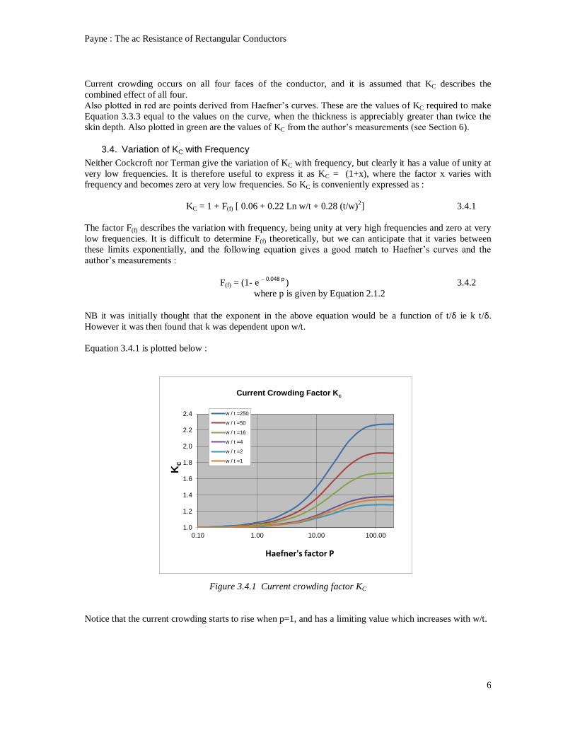
Figure 3.4.1 Current crowding factor KC

Notice that the current crowding starts to rise when p=1, and has a limiting value which increases with w/t.


7

0.0

0.2

0.4

0.6

0.8

1.0

1.2

0.0 0.5 1.0 1.5 2.0 2.5 3.0

t eff / t

δ/t

Effective Thickness t eff of Strip Conductor

t' / t

2δ

4. THEORY

4.1. Increase in R due to Crowding

Initially, assuming total diffusion into the conductor then the only increase in resistance from the dc

resistance will be due to current crowding, and then Equation 3.3.1 becomes (and putting A = wt) :

R = [ρ ℓ/(w t) ] KC 4.1.1

4.2. Diffusion loss

At high frequencies conduction will take place in only a thin band around the periphery, equivalent in depth

to the skin depth. This conduction will have therefore an area AHF =2 δ (w+t). Consider firstly a strip

conductor so the thickness is much smaller than the width and so the area becomes AHF ≈ 2 w δ. So the

effective thickness t’ changes from a value of t at low frequencies to 2δ at high frequencies.

Assuming that this has an exponential relationship gives :

t' = t (1- e

–2δ/t ) 4.2.1

At low frequencies teff is asymptotic to t, and at high frequencies teff is asymptotic to 2δ (the latter because e

x = 1+x +x

2/2! …. ≈ 1+x for small values of x).

Figure 4.2.1 Effective thickness of Strip conductor

In a thicker conductor diffusion will take place from 4 surfaces, and assuming that these four diffusions act

independently then the limiting value is equal to 2 δ/t + 2 δ/w = 2 δ/t (1+t/w). Equation 4.2.1 now becomes

:

t’ = t (1- e –x

) 4.2.2

x = 2 δ/t (1+t/w)

4.3. Overall Equation for all w/t ratios

So the ac resistance of a rectangular conductor is given by :

Rac = [ρ ℓ / (w t )] [ KC / (1- e –x

) ] 4.5.1


8

0.0

1.0

2.0

3.0

4.0

5.0

0.0 2.0 4.0 6.0 8.0 10.0 12.0 14.0

Rac

/Rd

c

Factor p

Rac/ Rdc w/t = 2

Calc Rac /Rdc

Haefner

0.0

1.0

2.0

3.0

4.0

0 2 4 6 8 10 12

Rac

/Rd

c

Factor p

Rac/ Rdc w/t = 1

Calc Rac /Rdc

Haefner

where ρ is the resistivity of the conductor

ℓ is the length of the conductor in metres

KC = 1 + F(f) [ 0.06 + 0.22 Ln w/t + 0.28 (t/w)2]

F(f) = (1- e – 0.048 p

) where p is given by Equation 2.1.2

x= 2(1+t/w) δ/t

δ = [ρ/(πfµ)]0.5

(= 66.6/f 0.5

for copper)

w is the width of the conductor in metres

t is its thickness in metres

ρ is the material resistivity in Ωm (= 1.72 10-8

for copper)

f is the frequency in Hz

It is useful to normalise this ac resistance to the dc resistance Rdc = ρ ℓ / (wt) to give the ratio Rac / Rdc :

Rac / Rdc = KC / (1- e –x

) 4.5.2

5. COMPARISON WITH HAEFNER’S CURVES

5.1. Comparison with theory

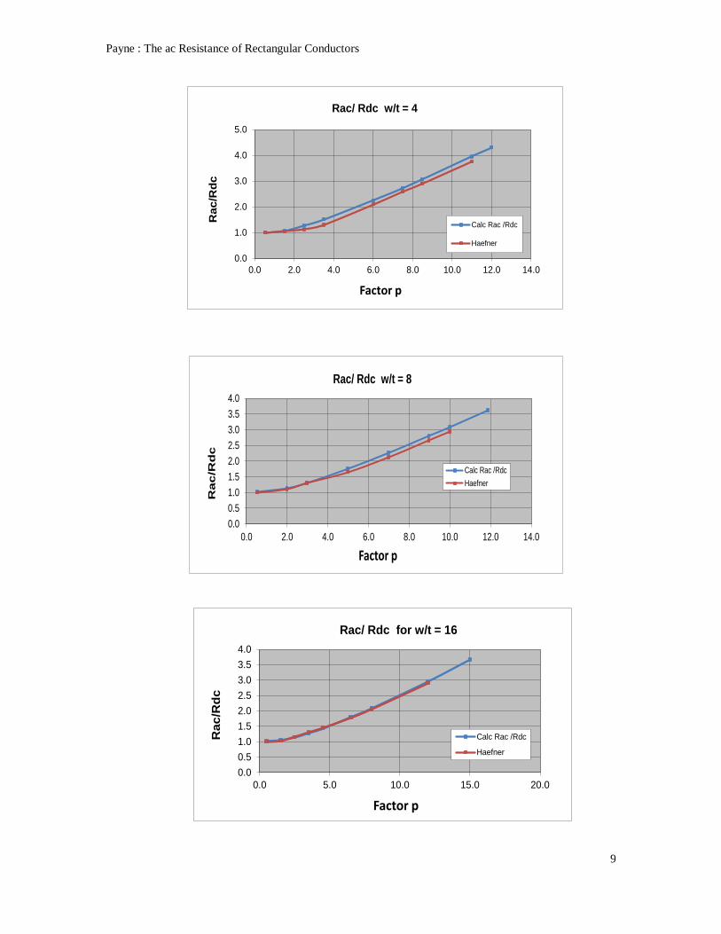
The comparison of Equation 4.5.2 with Haefner’s curves is given below :


9

0.0

1.0

2.0

3.0

4.0

5.0

0.0 2.0 4.0 6.0 8.0 10.0 12.0 14.0

Rac

/Rd

c

Factor p

Rac/ Rdc w/t = 4

Calc Rac /Rdc

Haefner

0.0

0.5

1.0

1.5

2.0

2.5

3.0

3.5

4.0

0.0 2.0 4.0 6.0 8.0 10.0 12.0 14.0

Rac

/Rd

c

Factor p

Rac/ Rdc w/t = 8

Calc Rac /Rdc

Haefner

0.0

0.5

1.0

1.5

2.0

2.5

3.0

3.5

4.0

0.0 5.0 10.0 15.0 20.0

Rac

/Rd

c

Factor p

Rac/ Rdc for w/t = 16

Calc Rac /Rdc

Haefner


10

0.8

1.0

1.2

1.4

1.6

0.0 2.0 4.0 6.0 8.0 10.0

Ra

c/R

dc

Factor p

Rac/ Rdc w/t =2400

Calc Rac /Rdc

Haefner

0.0

0.5

1.0

1.5

2.0

2.5

3.0

0.0 2.0 4.0 6.0 8.0 10.0 12.0 14.0

Ra

c/R

dc

Factor p

Rac/ Rdc w/t =24

Calc Rac /Rdc

Haefner

In the above graph for w/t =24 the slope of Haefner’s curve is less than the theoretical. However Haefner’s

curve is an extrapolation above p =5 and therefore may not be accurate.

The above data for w/t=2400 comes from Haefner’s original paper.


11

0.5

1.0

1.5

2.0

2.5

3.0

0 2 4 6 8 10 12 14 16 18 20 22 24

Resis

tan

ce r

ati

o

Haefner Factor p

Resistance ratio of Copper Strip w/t = 128

Measured Corrected Rac /Rdc

Theoretical Rac/Rdc

0.5

1.0

1.5

2.0

2.5

3.0

0 2 4 6 8 10 12 14 16

Resis

tan

ce r

ati

o

Haefner Factor p

Resistance ratio of Copper Strip w/t = 128

Measured Corrected Rac /Rdc

Theoretical Rac/Rdc

6. COMPARISON WITH AUTHOR’S MEASUREMENTS

6.1. w/t = 128

The ac resistance of a thin copper strip was measured. It was 7 metres long with a width of 5.1 mm, and a

measured thickness of 0.04 mm. This very small thickness is difficult to measure accurately and the

uncertainty was probably ±10%.

The following was measured (blue curve) :

Figure 6.1.1 Author’s measurements on Copper strip with w/t =128

Correlation with the theoretical curve is poor. However measurements of the dc resistance of the copper

strip showed that its resistivity was 2.75 10-8

Ωm compared with that of pure copper of 1.72 10-8

Ωm. This

indicated that it contained impurities and these increased its permeability above unity as a test showed (see

Appendix 3). Nickle is the most likely impurity because it improves the corrosion resistance, and the

percentage needed to explain the raised resistivity was calculated to be 1.07%, raising the permeability to

2.2 (Appendix 4). If the skin depth in Equation 2.1.2 is calculated with this value of permeability the

Haefner factor p changes for each of the measurement frequencies and the correlation with the theoretical

improves to :

Figure 6.1.2 Comparison with µr = 2.2

The good correlation here is probably fortuitous because the measurements are subject to considerable error

because the values were less than 2Ω. However there is definitely a different slope and this is also apparent

in some of the comparisons with Haefner’s curves, so this may indicate a limitation of the theory.


12

0

1

2

3

4

5

0 1 2 3 4 5 6 7 8 9 10 11 12

Ra

c /

Rd

c

Haefner Factor p

Resistance of Copper Strip w/t = 1

Measured Corrected Rac /Rdc w/t = 1

Theoretical Rac/Rdc

Haefner w/t=1

0

1

2

3

4

5

0 2 4 6 8 10 12 14 16

Rac /

Rd

c

Haefner Factor p

Resistance of Thin Flat Bronze Strip w/t = 14

Measured Corrected Rac /Rdc w/t = 14

Theoretical Rac/Rdc

Haefner w/t=16

6.2. w/t =14

Measurements were made of a bronze strip of width 2.46 mm and thickness of 0.18 mm, so having w/t =

14. The resistivity was determined as ρ = 12 10-8

by measuring the dc resistance of a 3 meter length.

Appendix 1 gives the experimental details. The metal was found to be very slightly magnetic (Appendix 3),

and so the skin depth was calculated on the assumption that µr =1.1.

These measurements are compared with Equation 4.5.2 below :

Figure 6.2.1 Comparison between author’s measurement and theory for w/t = 14

The resistance values were very low at less than 2Ω over most of the frequency range from 0.01 to 25 MHz,

and the measurement error is assessed as ±10%.

Self–resonance determined the maximum frequency which could be measured (see Appendix 2) and this

frequency is dependent upon the length of the conductor. So a 6 metre length was used for measurements

between 0.01 and 0.5 MHz, and a 1.5 metre length for 0.5 to 20 MHz.

6.3. w/t = 1

Also measured was a square bronze conductor of sides 0.69 mm, with two lengths of 6 m and 1.5 m. The

resistivity was determined as ρ = 16 10-8

by measuring the dc resistance of a 6 meter length.

These measurements are compared with Equation 4.5.2 below :

Figure 6.3.1 Comparison between author’s measurement and theory for w/t=1


13

Measurement error was somewhat less here because the resistance was higher at between 2 and 8 Ω. The

measurements are seen to lie very close to both the Haefner curve and the theoretical curve, and so the

marker points have been made especially large to make them visible.

7. SUMMARY AND CONCLUSIONS

It is shown that Equation 4.5.1 gives a very good prediction of the resistance of rectangular conductors,

from thin strip to square cross-section and over a frequency range from dc up to high frequencies.


14

Appendix 1 : EXPERIMENTAL DETAILS

All resistance measurements were made with an Array Solutions UHF Vector Network Analyser.

Calibration of this analyser required an open circuit, a short circuit and known resistive load, and these are

shown below.

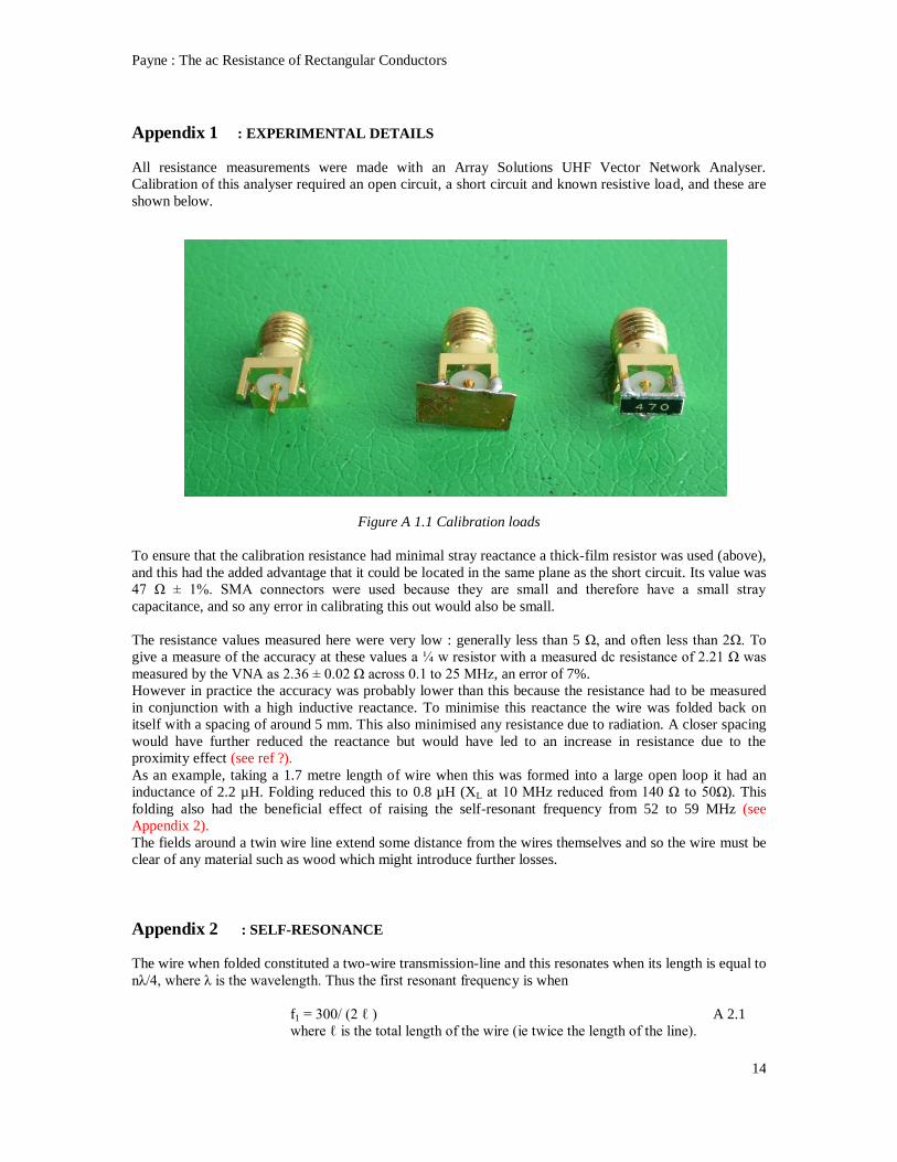
Figure A 1.1 Calibration loads

To ensure that the calibration resistance had minimal stray reactance a thick-film resistor was used (above),

and this had the added advantage that it could be located in the same plane as the short circuit. Its value was

47 Ω ± 1%. SMA connectors were used because they are small and therefore have a small stray

capacitance, and so any error in calibrating this out would also be small.

The resistance values measured here were very low : generally less than 5 Ω, and often less than 2Ω. To

give a measure of the accuracy at these values a ¼ w resistor with a measured dc resistance of 2.21 Ω was

measured by the VNA as 2.36 ± 0.02 Ω across 0.1 to 25 MHz, an error of 7%.

However in practice the accuracy was probably lower than this because the resistance had to be measured

in conjunction with a high inductive reactance. To minimise this reactance the wire was folded back on

itself with a spacing of around 5 mm. This also minimised any resistance due to radiation. A closer spacing

would have further reduced the reactance but would have led to an increase in resistance due to the

proximity effect (see ref ?).

As an example, taking a 1.7 metre length of wire when this was formed into a large open loop it had an

inductance of 2.2 µH. Folding reduced this to 0.8 µH (XL at 10 MHz reduced from 140 Ω to 50Ω). This

folding also had the beneficial effect of raising the self-resonant frequency from 52 to 59 MHz (see

Appendix 2).

The fields around a twin wire line extend some distance from the wires themselves and so the wire must be

clear of any material such as wood which might introduce further losses.

Appendix 2 : SELF-RESONANCE

The wire when folded constituted a two-wire transmission-line and this resonates when its length is equal to

nλ/4, where λ is the wavelength. Thus the first resonant frequency is when

f1 = 300/ (2 ℓ ) A 2.1

where ℓ is the total length of the wire (ie twice the length of the line).


15

As this frequency is approached the measured resistance and the inductance increase above their true value

and Welsby ( ref 5, p 37) has shown that the true value is given by :

L = LM [ 1- (f / fR )2] A2.2

R = RM [ 1- (f / fR )2]2 A2.3

LM and RM are the measured values, and fR is the self-resonant frequency. Welsby developed these

equations for the self-resonance in coils and experience shows that they are applicable to open wire lines if

Equation A 2.1 is modified to :

Open wire fR = 300/ (3 ℓ ) A 2.4

where ℓ is the total length of the wire (ie twice the length of the line).

However these equations become increasingly inaccurate as the resonant frequency is approached and

should not be used above about fR/3 (at which frequency the correction is about 30% for resistance).

Appendix 3 : TEST FOR PERMEABILITY OF COPPER

A short length of the copper strip was placed onto the surface of water contained in a glass cup, supported

by surface tension. A permanent magnet was brought close and the copper strip drifted very slowly towards

it taking around 5 minutes to traverse the diameter of the glass. This showed that the permeability of the

strip was greater than unity but the slow movement suggests that it was probably not much greater than

unity, and indeed the permeability was not so high that conductor would ‘stick’ to a powerful permanent

magnet.

Figure A3.1 Permeability test


16

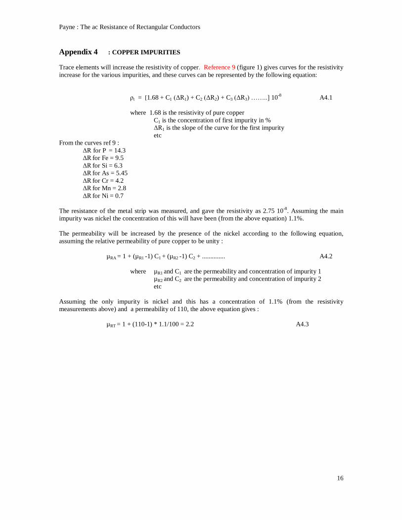
Appendix 4 : COPPER IMPURITIES

Trace elements will increase the resistivity of copper. Reference 9 (figure 1) gives curves for the resistivity

increase for the various impurities, and these curves can be represented by the following equation:

ρt = [1.68 + C1 (ΔR1) + C2 (ΔR2) + C3 (ΔR3) ……..] 10-8

A4.1

where 1.68 is the resistivity of pure copper

C1 is the concentration of first impurity in %

ΔR1 is the slope of the curve for the first impurity

etc

From the curves ref 9 :

ΔR for P = 14.3

ΔR for Fe = 9.5

ΔR for Si = 6.3

ΔR for As = 5.45

ΔR for Cr = 4.2

ΔR for Mn = 2.8

ΔR for Ni = 0.7

The resistance of the metal strip was measured, and gave the resistivity as 2.75 10-8

. Assuming the main

impurity was nickel the concentration of this will have been (from the above equation) 1.1%.

The permeability will be increased by the presence of the nickel according to the following equation,

assuming the relative permeability of pure copper to be unity :

µRA = 1 + (µR1 -1) C1 + (µR2 -1) C2 + .............. A4.2

where µR1 and C1 are the permeability and concentration of impurity 1

µR2 and C2 are the permeability and concentration of impurity 2

etc

Assuming the only impurity is nickel and this has a concentration of 1.1% (from the resistivity

measurements above) and a permeability of 110, the above equation gives :

µRT = 1 + (110-1) * 1.1/100 = 2.2 A4.3


17

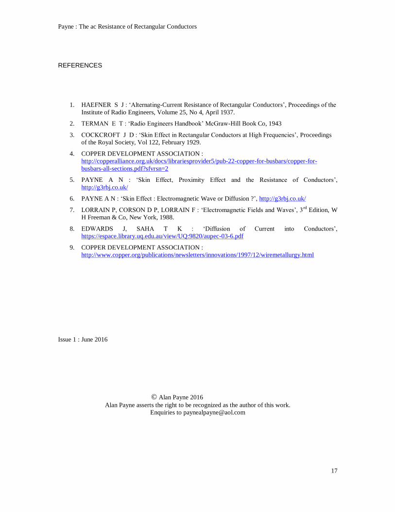
REFERENCES

1. HAEFNER S J : ‘Alternating-Current Resistance of Rectangular Conductors’, Proceedings of the

Institute of Radio Engineers, Volume 25, No 4, April 1937.

2. TERMAN E T : ‘Radio Engineers Handbook’ McGraw-Hill Book Co, 1943

3. COCKCROFT J D : ‘Skin Effect in Rectangular Conductors at High Frequencies’, Proceedings

of the Royal Society, Vol 122, February 1929.

4. COPPER DEVELOPMENT ASSOCIATION :

http://copperalliance.org.uk/docs/librariesprovider5/pub-22-copper-for-busbars/copper-for-

busbars-all-sections.pdf?sfvrsn=2

5. PAYNE A N : ‘Skin Effect, Proximity Effect and the Resistance of Conductors’,

http://g3rbj.co.uk/

6. PAYNE A N : ‘Skin Effect : Electromagnetic Wave or Diffusion ?’, http://g3rbj.co.uk/

7. LORRAIN P, CORSON D P, LORRAIN F : ‘Electromagnetic Fields and Waves’, 3rd

Edition, W

H Freeman & Co, New York, 1988.

8. EDWARDS J, SAHA T K : ‘Diffusion of Current into Conductors’,

https://espace.library.uq.edu.au/view/UQ:9820/aupec-03-6.pdf

9. COPPER DEVELOPMENT ASSOCIATION :

http://www.copper.org/publications/newsletters/innovations/1997/12/wiremetallurgy.html

Issue 1 : June 2016

© Alan Payne 2016

Alan Payne asserts the right to be recognized as the author of this work.

Enquiries to [email protected]

http://copperalliance.org.uk/docs/librariesprovider5/pub-22-copper-for-busbars/copper-for-busbars-all-sections.pdf?sfvrsn=2

http://copperalliance.org.uk/docs/librariesprovider5/pub-22-copper-for-busbars/copper-for-busbars-all-sections.pdf?sfvrsn=2

http://g3rbj.co.uk/

http://g3rbj.co.uk/

https://espace.library.uq.edu.au/view/UQ:9820/aupec-03-6.pdf

http://www.copper.org/publications/newsletters/innovations/1997/12/wiremetallurgy.html

Resistance of rectangular conductors - G3RBJ |...

Documents

Transcript of Resistance of rectangular conductors - G3RBJ |...