Reservoir performance and dynamic managementunder plausible assumptions of future climateover seasons to decades

M. Neil Ward & Casey M. Brown & Kye M. Baroang &

Yasir H. Kaheil

Received: 17 January 2012 /Accepted: 9 October 2012# Springer Science+Business Media Dordrecht 2012

Abstract An analysis procedure is developed to explore the robustness and overall produc-tivity of reservoir management under plausible assumptions about climate fluctuation andchange. Results are presented based on a stylized version of a multi-use reservoir managementmodel adapted from Angat Dam, Philippines. Analysis focuses on October-March, duringwhich climatological inflow declines as the dry season arrives, and reservoir managementbecomes critical and challenging. Inflow is assumed to be impacted by climate fluctuationsrepresenting interannual variation (white noise), decadal to multidecadal variability (MDV, hererepresented by a stochastic autoregressive process) and global change (GC), here representedby a systematic linear trend in seasonal inflow total over the simulation period of 2008–2047.Stochastic (Monte Carlo) simulations are undertaken to explore reservoir performance. In thisway, reservoir reliability and risk of extreme persistent water deficit are assessed in the presenceof different combinations and magnitudes of GC and MDV. The effectiveness of dynamicmanagement is then explored as a possible climate change adaptation practice, focusing onreservoir performance in the presence of a 20 % downward inflow trend. In these dynamicmanagement experiments, the October-March water allocation each year is adjusted based onseasonal forecasts and updated climate normals. The results illustrate how, in the near-term,MDV can be as significant as GC in impact for this kind of climate-related problem. The results

Climatic ChangeDOI 10.1007/s10584-012-0616-0

Electronic supplementary material The online version of this article (doi:10.1007/s10584-012-0616-0)contains supplementary material, which is available to authorized users.

M. N. Ward (*)Independent Scholar, Basking Ridge, NJ 07920, USAe-mail: mneilward@gmail.com

C. M. BrownDepartment of Civil and Environmental Engineering, University of Massachusetts, Amherst, MA 01003,USA

K. M. BaroangEarth Institute at Columbia University, New York, NY 10025, USA

Y. H. KaheilRisk Management Solutions, Newark, CA 94560, USA

also illustrate how dynamic management can mitigate the impacts. Overall, this type of analysiscan deliver guidance on the expected benefits and risks of different management strategies andclimate scenarios.

AbbreviationsAR AutoregressiveDA Dynamic AllocationENSO El Niño Southern OscillationGC Global ChangeJAS July-SeptemberJFM January-MarchMCD Maximum Cumulative DeficitMCM Million Cubic MetersMDV Multidecadal VariabilityOND October-DecemberONDJFM October-MarchSA Static Allocation

1 Introduction

One of the key challenges in the presence of climate change is how to better connect climateimpact knowledge to adaptation actions. This is especially critical for local scale climate-relatedproblems, such as the one addressed in this paper, themanagement of a multi-use reservoir with arelatively modest catchment area, yet serving 11 million urban residents and irrigation for anestimated 40,000 farms. There are a number of approaches being explored to enhance theconnection of impact knowledge with adaptation (e.g., Mastrandrea et al. 2010), with often akey component being stakeholder-science interaction. Partly as a result of such interactions, oneapproach is the development of plausible future climate scenarios, to assess the robustness ofadaptation strategies across a range of possible climate outcomes (Dessai et al. 2009; Groves etal. 2008). Such assessments provide valuable background for decision makers to find the bestcompromise strategies in the absence of detailed quantified climate change predictions (Lempertet al. 2006; Lempert and Collins 2007).

This paper aims to contribute by developing and demonstrating a framework for such ananalysis. The context is a stylized (i.e., simplified for illustration) multi-purpose reservoirmodel, based on the Angat system in the Philippines (Brown et al. 2009). The model focuseson the monthly operations related to water supply; daily flood control and hydroelectricityreleases are not addressed. In addition to the general framework, two particular aspects arehighlighted that have often not been previously emphasized in integrated quantitativesystems such as presented here. Firstly, in addition to a plausible global change (GC)component, we also stochastically introduce natural decadal to multidecadal variability(MDV) into the inflow traces that are used to explore reservoir sensitivity. Early studiesrecognized the potential impact of MDVon water resources (e.g., Lall and Mann 1995). Thenature of MDV varies with geographical region (e.g., Meehl et al. 2009), but in manylocations it is now believed to be large enough to be a significant compounding factor on topof GC for climate risk in reservoir management. This is especially the case for near-termclimate perspectives that many stakeholders seek. Thus, the simulation framework in thispaper assesses the robustness of a reservoir management system, in the presence of GCalone, and in combination with MDV, over a 40-year timeframe into the future.

Climatic Change

Secondly, the simulation framework includes choices about continuous year-on-year man-agement, since this alters the robustness of a reservoir to climate change. One of those choices isthe incorporation of seasonal climate forecasts. The potential of such forecasts in general for theAngat reservoir is discussed in Brown et al. (2009). The focus now is seasonal forecast use andreservoir robustness in the presence of climate trends. A further source of information that maybe drawn upon to adjust management strategy each year is updates of the best estimate of thelow-frequency climate state (i.e., an attempt to track any emerging trends and use this to estimatethe expected climate for the coming year) (e.g., Livezey et al. 2007; Arguez and Vose 2011; andapplication example discussed in Siebert and Ward 2011). We illustrate incorporation of bothseasonal predictions and updated climate normals, as options to potentially increase resilience inthe presence of climate change.

Actions that reduce sensitivity to climate are recognized as a potential component ofadaptation (Mastrandrea et al. 2010). By having in place systems that are flexible and able torespond to real-time monitoring over weeks to months, and/or short-term seasonal forecasts,society can take on actions that, over time, are better able to cope with the new emergingclimate patterns. While such enhanced management of climate variability is now widelyacknowledged to be a contributor to adaptation (e.g., UNDP 2002; Meinke and Stone 2005;Klopper et al. 2006; Ziervogel et al. 2010), the extent of the contribution remains to beproven (Someshwar 2008). There are well-documented constraints to establishing flexiblerisk management systems for climate variability, including in the water sector (Lemos et al.2002; Rayner et al. 2005), but also examples of progress (Pagano and Garen 2006; Feldmanand Ingram 2009). The simulation approach in this paper is intended to partly provide aframework to better explore the potential role of adaptive management, while at the sametime, providing information that better informs stakeholders of the implications of differentchoices under plausible scenarios of climate variability and change, thereby contributing tothe science-stakeholder dialogue.

A special case is the role of climate extremes. Long-term livelihood, macro-economic andbiophysical impact can result from an individual climate extreme or run of extremes (Barrettet al. 2007; Carter et al. 2007; Akhtar 1998; UNEP 2007). The nature of the seasonal storageand re-charge in the reservoir modeled here is such that the level of the reservoir is re-seteach year. Thus there is no long-lasting biophysical finger-print of an extreme drought in thephysical system being modeled. In reality, there are still potential long-lasting economic/livelihood impacts of extreme years or runs of extremes. Therefore, a metric is introduced(cumulative water deficit statistic) to serve as a proxy for monitoring the frequency andmagnitude of high impact situations.

Section 2 introduces the framework and methodology. Section 3.1 illustrates a sensitivityanalysis across different plausible climate scenarios, holding management strategy constantover the simulation period of 2008–2047. Section 3.2 illustrates, for a single case studyrealization, how the sensitivities alter when reservoir management is allowed to respondeach year (over the 2008–2047 period) to climate-based expectations about the comingseasonal inflow. Section 4 provides discussion and conclusions.

2 Data, methodology and preparatory analysis

2.1 Reservoir management

The hydroclimatic setting used follows the actual circumstances found for the Angat reservoirin the Philippines. The drainage basin feeding the reservoir covers 586 km2 and the annual

Climatic Change

average inflow is 1893 million cubic meters (mcm). Inflow is strongly tied to rainfall, with highinflow occurring during October-December (OND), and much lower inflow during January-March (JFM) as the dry season becomes established. For the analysis in this paper, the reservoirmanagement problem is collapsed to a two-user system over the October-March (ONDJFM)period, with a primary user (municipal) and a secondary user (agriculture)1.

The existence of an El Niño Southern Oscillation (ENSO) connection with the region’sclimate in OND (e.g., Lyon and Camargo 2009), leads to a basis for OND reservoir inflowpredictions that can potentially be used to enhance reservoir management. Given this, andthe fact that OND dominates the ONDJFM variability (Online Resource 2), perturbations toinflow (trend, MDV, updated climate normals, seasonal forecasts) are always confined toOND in this study. Where needed by the reservoir model, the historical climatological JFMvalues and their distribution are used in all analyses. The OND and JFM values for 1968–2007 (provided by the Philippines National Power Corporation and plotted in OnlineResource 2), contain no significant trends, and their distribution is not significantly differentfrom normal.

In the reservoir management model, a monthly water allocation (October through March)is made to each user at the beginning of October. There are two reservoir managementapproaches assessed in this analysis: static allocation (SA), where the allocations are thesame each year, and dynamic allocation (DA), where allocation is allowed to vary each yearbased on best-estimate climate expectations for the coming seasonal inflow (e.g., seasonalforecast or updated climate normal). Simulations of reservoir performance are undertaken inthe presence of different climate variability and change scenarios over the period 2008–2047. For all the SA runs reported in Section 3.1, the monthly allocations are held constant,following a set of municipal and agriculture allocations that represent an initial typical targetin the Angat system (Online Resource 3). The SA results (Section 3.1) therefore serve tohighlight the sensitivity of a specific fixed water allocation strategy to different assumptionsabout climate variability and change. In contrast, the DA simulations (Section 3.2) areexamples of dynamic management. The dynamic approach may contribute to making thereservoir more robust in the presence of climate variability and change.

First, we discuss the design of the SA experiments. For each SA experiment year, thesimulation steps through each month from October to March. Inflow to the reservoir eachmonth is specified by the climate scenario, while the reservoir is drawn down each monthaccording to the allocations. Performance assessments here focus on the end of seasonreservoir water volume. The reservoir has a minimum acceptable volume (Vc) at the end ofMarch, based on the amount of water needed to satisfy demand throughout the remainder ofthe dry season. We calculate:

V 0i ¼ Vi � Vc ð1Þ

where Vi is the end of March volume in simulation i and Vc is the lower rule curve volume of348 mcm. The percentage of times that V’ is positive is referred to as the reservoir reliability.When V’ is negative, the outcome implies a water deficit. The average deficit in deficit years isoften referred to as reservoir vulnerability (Hashimoto et al. 1982). The opposite managementproblem of water excess, is summarized through statistics about reservoir spilling. For this, V’ iscompared to the 663 mcm spill threshold (based on the operational spill rule), to assess if andhow much water to consider as being spilled in the given simulation.

1 Further technical details of the reservoir, the management model, and the techniques for generating inflowscenarios, can be found in Online Resource 1 (text) and Online Resource 2 (figures).

Climatic Change

We also wished to introduce and illustrate a performance measure that captures the risk ofan extreme outcome that may have long-lasting impacts, such as a run of consecutive yearswith water deficits. To provide such a measure, conditions during 2038–2047 are focusedupon, when imposed trends will be having maximum expression. For simulation i during2038–2047, runs of consecutive years with V’ negative are identified. For each run of years,the cumulative value of V’ is calculated. The maximum cumulative value is termed themaximum cumulative deficit (MCD) for simulation i.

To give an indication of the risk of large cumulative deficits, the 90th percentile of theMCD is presented (MCD90). This is estimated by ranking the MCD values that arecalculated in each Monte Carlo simulation set, and taking the 90th ranked value. For theselected climate scenario combination (MDV and GC), there is therefore a 10 % risk ofhaving a cumulative deficit equal to or greater than MCD90 during 2038–2047. This type ofmeasure is considered to provide valuable additional information in the assessment ofreservoir performance under alternate climate scenarios.

Next, we discuss the additional aspects needed for the DA simulations. In the DAsimulations, the allocation amounts assigned at the beginning of October are allowed tovary each year according to the expected inflow for the coming ONDJFM period. In thispaper, ENSO-based inflow forecasts and updated climate normals (also referred to asupdated climatology) are explored as tools that can improve water allocations.

For the DA simulations, 90 % reservoir volume reliability (based on Eq. 1) is targeted foreach year. Each year has a unique allocation solution based on the expected inflow (meanand standard deviation). Using a numerical iteration procedure, the total amount of waterallocated is gradually increased until, sampling from the expected distribution of reservoirinflows, the reservoir volume is estimated to have a 10 % chance of being below Vc at theend of March. Once a total allocation amount is identified, it is allocated to the two usersaccording to the priority system: first, the basic municipal demand (722 mcm) is met to theextent possible; then agriculture receives the remaining allocation (if any). Once a seasonalallocation is made, it is sub-divided into months maintaining the same constant proportionaldistribution.

2.2 Inflow for the SA simulations

There are potentially many useful ways to generate plausible inflow scenarios, and thepurpose here is not to promote the details of a particular simulation methodology. Rather, theaim is to choose a set of methods that yield reasonable and transparent inflow scenarios, withwhich to illustrate the types of insights that can be gained from the approach.

All simulations are for the 40-year period 2008–2047, and they are considered a contin-uation of the historical 1968–2007 inflow record. We make assumptions about the character-istics of interannual variability, MDV2 and GC, and assume they are linearly expressed in thefuture inflow series. Interannual variability and MDV are generated using Monte Carlosimulation (100 for each experiment3, i.e. for each combination of MDV and GC that istested), while GC is imposed systematically as a linear trend, corresponding to x% change ininflow over 2008–2047. The intention is to explore sensitivity to trends of magnitudes that

2 Sources of MDV in the climate system include the Atlantic Multidecadal Oscillation and the Pacific DecadalOscillation, e.g., see Meehl et al. 2009 and Online Resource 1.3 The choice of sample size 100 was found to be sufficient to illustrate general tendencies in the illustrativeresults presented. Larger Monte Carlo sample size will give more precise estimates and should be consideredwhen seeking to draw definitive conclusions about any given system.

Climatic Change

are plausible given the GC processes that are underway (Solomon et al. 2007). Forillustration in this study, the range of inflow changes explored is +/− 20 %.

For scenarios with trend and interannual variability, a smooth trend of specified magni-tude has superimposed upon it, interannual variability sampled from a normal distributionthat has mean and standard deviation equal to that found in the historical OND inflowrecord. For scenarios with MDV, the MDV is assumed to follow a first order autoregressive(AR) process, tuned such that the mean and variance of the process is consistent with thehistorical inflow values for Angat. The lag 1 autocorrelation (r1) in the AR model defines theextent of MDV present in the simulated series, which here always have one value per year,hence lag is for a 1-year time step. Setting r100.6 (so persistence of inflow from 1 year to thenext will explain 36 % of the variance of the inflow series), Siebert and Ward (2011) discusshow simulations resemble quite well the type of variations seen in some of the morepersistent climate series, such as for the Sahel region of Africa. It turns out that the Angatbasin is located in a region that has not experienced strong MDV in recent decades (e.g., Lyonand Camargo 2009). Nonetheless, the stylized reservoir management model can be subjected toinflows that contain MDV, to explore and illustrate sensitivities to this type of climatefluctuation.

In reality, water systems will experience both GC and MDV simultaneously, and it istherefore valuable to assess the sensitivity of reservoir management when inflow traces containa representation of both GC andMDV. To achieve such traces, the AR process traces (represent-ingMDV) have a time-series of adjustments added that would correspond to the introduction of asmooth linear trend of specified magnitude. For example, Fig. 1a provides a sample of the rangeof outcomes that are possible over a 40-year period, for a given location where GC processes areassumed to be driving a 20 % downward trend in inflow, and MDV processes are assumed to beoperating at a magnitude leading to r100.6. Once the seasonal inflow totals are simulated (e.g.,the series in Fig. 1a), sub-component monthly inflow values (needed to drive the reservoirmodel) are created by maintaining the climatological month-to-month ratios.

2.3 Inflow for the DA simulations

Since this is a more complex system to construct, the initial illustration here has been confinedto climate trend scenarios of no change and a 20 % downward trend. Furthermore, results arealso confined to a single case study realization of interannual variability. A number of additionalinflow features must be calculated in order to perform the DA experiments. First, to obtainOND inflow values based on seasonal forecasts, a cross-validated (leave-one-out) univariateregression is performed between OND inflow and July-September (JAS) Niño3.4 over 1968–2007. The pairs of forecast-observed values are then scrambled to give a scenario of forecast-observed values for 2008–2047 (Fig. 1b; for more details of all DA inflow series, see OnlineResource 1). Forecast and observed scenarios that contain a 20 % downward trend aregenerated by linearly adjusting the raw values (also plotted in Fig. 1b).

To obtain OND inflow values based on a simple updated climatology, a 30-year runningmean window is applied. The updated climate normal for year i (green line Fig. 1b) is basedonly on information available up to year i−1 (i.e., the average of the previous 30 years). Inestimating the updated climatology, 1968–2007 is assumed to be stationary, so values forthose years always take the 1968–2007 climatological inflow value.

An intermediate assumption for seasonal forecast trend is to assume that the seasonalforecasts could at least be adjusted each year by the updated climate normal estimate. Thisyields a third set of seasonal forecasts (not shown) that have a trend consistent with theupdated climatology.

Climatic Change

For each year in any given DA simulation, we generate 1,000 inflow values4 drawingfrom a distribution defined by the expected inflow and associated standard deviation. Theseinflow values are used with the reservoir model to estimate the water allocation thatcorresponds to 90 % reservoir reliability. Finally, to serve as a base-line for comparison,5,000 inflows were sampled from the climatological ONDJFM distribution, to permit robustestimation of the water allocation corresponding to 90 % reliability using climatologicalinformation (i.e., the static allocation that achieves 90 % reliability over 1968–2007). Thiswas estimated at 920 mcm.

3 Results

3.1 Static allocation (SA experiments)

The evolution of average reliability under a range of GC trends is shown in Fig. 2a (more detailsare in Online Resource 3, including discussion of statistical validity). By 2048, a +20% trend in

4 The choice of sample size 1,000 was found to be sufficient here to reveal general patterns. In other situations,larger sample sizes may be needed depending on desired precision.

Fig. 1 a 40-year simulations of October-December inflow. These are examples of the inflow series used inthe SA experiments. The simulation model assumes a combination of random MDV (AR process r100.6) andsystematic downward trend (20 % over 40 years). A linear trend was fit to each of 100 simulations. The seriesshown were selected to give a representative sample of trend sizes. For the series with trend size ranking 10 %and 90 %, the linear trend line is also plotted (thick black lines). b Creating seasonal forecast-observed inflowscenarios for 2008–2047. These inflow series are drawn on in the DA experiments. Seasonal inflow forecastsare in blue and corresponding observations are in red. The thick solid lines show a random rearrangement ofthe OND seasonal forecast-observed pairs for 1968–2007 (correlation skill r00.55). The thin blue and redlines are the same forecast-observed pairs, but now with a 20 % downward trend. The updated climate normal(i.e., updated climatology of inflow, green line) tracks the emerging downward trend in the thin red line

Climatic Change

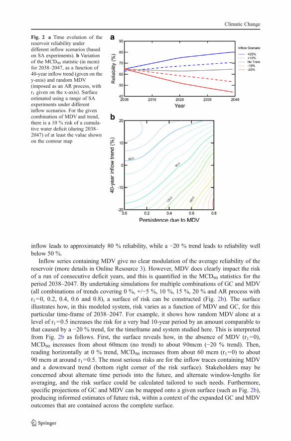
inflow leads to approximately 80 % reliability, while a −20 % trend leads to reliability wellbelow 50 %.

Inflow series containing MDV give no clear modulation of the average reliability of thereservoir (more details in Online Resource 3). However, MDV does clearly impact the riskof a run of consecutive deficit years, and this is quantified in the MCD90 statistics for theperiod 2038–2047. By undertaking simulations for multiple combinations of GC and MDV(all combinations of trends covering 0 %, +/−5 %, 10 %, 15 %, 20 % and AR process withr100, 0.2, 0.4, 0.6 and 0.8), a surface of risk can be constructed (Fig. 2b). The surfaceillustrates how, in this modeled system, risk varies as a function of MDV and GC, for thisparticular time-frame of 2038–2047. For example, it shows how random MDV alone at alevel of r100.5 increases the risk for a very bad 10-year period by an amount comparable tothat caused by a −20 % trend, for the timeframe and system studied here. This is interpretedfrom Fig. 2b as follows. First, the surface reveals how, in the absence of MDV (r100),MCD90 increases from about 60mcm (no trend) to about 90mcm (−20 % trend). Then,reading horizontally at 0 % trend, MCD90 increases from about 60 mcm (r100) to about90 mcm at around r100.5. The most serious risks are for the inflow traces containing MDVand a downward trend (bottom right corner of the risk surface). Stakeholders may beconcerned about alternate time periods into the future, and alternate window-lengths foraveraging, and the risk surface could be calculated tailored to such needs. Furthermore,specific projections of GC and MDV can be mapped onto a given surface (such as Fig. 2b),producing informed estimates of future risk, within a context of the expanded GC and MDVoutcomes that are contained across the complete surface.

Fig. 2 a Time evolution of thereservoir reliability underdifferent inflow scenarios (basedon SA experiments). b Variationof the MCD90 statistic (in mcm)for 2038–2047, as a function of40-year inflow trend (given on they-axis) and random MDV(imposed as an AR process, withr1 given on the x-axis). Surfaceestimated using a range of SAexperiments under differentinflow scenarios. For the givencombination of MDV and trend,there is a 10 % risk of a cumula-tive water deficit (during 2038–2047) of at least the value shownon the contour map

Climatic Change

The approach in this section allows the assessment of a current management system underdifferent climate scenarios, and informs stakeholders of system vulnerabilities. Once such aframework is constructed, modifications can be assessed as possible adaptation strategies,including alternate infrastructure configurations and alternate operational management, suchas water allocation. Usually, the latter assumes the same allocation will be made each year.The next section introduces analysis of a further consideration: the extent to which sensitivitiesto climate might be reduced when allocation is allowed to vary each year, based on expectationsfor the upcoming season’s inflow.

3.2 Dynamic allocation (DA experiments)

Results in this section illustrate vulnerability analyses for the no trend climate scenario andthe 20 % downward trend climate scenario (more detailed results are in Online Resource 4).First, a baseline SA result is produced for comparison with the adaptive management DAapproaches. SA in the presence of a 20 % downward inflow trend results in a gradual declinein V’ (Fig. 3a, blue line). This finds expression in the summary statistics (Online Resource 4)such as deficit frequency (increasing from 5/40 to 7/40) and maximum deficit (increasingfrom 281 mcm to 406 mcm). The following results provide an illustration of the extent towhich adaptive management can alter such sensitivity to climate trends.

In the presence of the downward 20 % inflow trend, water allocation based on updatedclimatology leads to much less downward trend in V’ (Fig. 3a, green line) compared to usingSA (Fig. 3a, blue line). The water allocation process gradually recognizes the downward

Fig. 3 End of March deficit/surplus (V’, negative values aredeficits). a Management usinghistorical climatology information(for observed of no inflow trendand observed of 20 % downwardinflow trend), and managementusing updated climate normals(for observed of 20 % downwardinflow trend), b Managementusing seasonal forecasts in thepresence of a 20 % downwardtrend in the observed inflow. Theseasonal forecasts are constructedto track the observed trend tovarying degrees. Note the red andblue lines in (a) are examples ofresults with SA management (i.e.,fixed allocation), while all otherresults are examples of DA forcomparison. Allocation for theseSA results targets 90 % reliabilityover 1968-2007 (climatologymanagement), whereas the DAresults target 90 % reliability forthe given year

Climatic Change

trend in inflow and therefore learns to manage the reservoir more conservatively (quantifiedand discussed in Online Resource 4). The overall impression in Fig. 3a is that responding toupdated climate normals can substantially contribute toward making the reservoir sustainable inthe presence of an inflow trend of this magnitude (at least in terms of allocations to avoidgrowing deficit problems).

Next, reservoir sensitivity is explored when seasonal forecasts are used to inform waterallocation. First, with no inflow trend, there emerge the known benefits of using seasonalforecasts (e.g., Brown et al. 2009). As shown in Online Resource 4, the reliability of thereservoir is maintained (deficit frequency 4/40) while more water is on average allocated tousers (977 mcmc with seasonal forecasts, 920 mcm based on climatological information),there is a lower average deficit (99 mcm v 122 mcm) and less spill. These results reflectgenerally correctly anticipating the low inflow years, and adjusting allocation to the down-side;and generally correctly anticipating high inflow years, and adjusting allocations substantiallyhigher. The net effect of the adjustments is to allow on averagemore water to be allocated while,nonetheless, keeping the likelihood of a deficit unchanged. A key question arises: to what extentare these positive attributes of reservoir performance compromised in the presence of a 20 %downward inflow trend?

Firstly, the best case scenario is considered, when seasonal forecasts fully track the observedtrend. For this case study, the performance is almost unaltered in terms of V’, deficit and spill(comparison is in Online Resource 4; V’ in the presence of the trend is shown in Fig. 3b redline). The reservoir is able to maintain its productivity and reliability, through a gradualadjustment in the allocation, responding to the downward trend in seasonal forecasts (i.e., theseasonal forecasts in Fig. 1b, thin blue line). The gradual adjustment is small compared to theallocation adjustments that are applied each year to manage the interannual climate variability(e.g., see Fig. 4 and the further discussion of allocation later in this section).

When the seasonal forecasts are not adjusted to track the inflow trend, many of thebenefits from seasonal forecasts do still remain (such as average increase in water allocated,and early warning of many of the drought years through low allocation). Nonetheless, V’ isgradually declining (Fig. 3b blue line; compare to the red line when seasonal forecasts dotrack the inflow trend) and the deficit frequency (8/40) for this case study realization isactually higher than using static allocation (blue line Fig. 3a, deficit frequency is 7/40).However, it is reasonable to assume that in many cases, seasonal forecasts could at leastcontain trend information from an updated climate normals approach. Using such seasonalforecasts to manage the reservoir gives a better performance in terms of deficit frequencyand average deficit (Online Resource 4, and visually apparent in Fig. 3b, green line, where

Fig. 4 Water allocation to user 2(agriculture) in the presence of a20 % downward trend in inflow.Allocations (DA analysis) arebased on seasonal forecasts withno trend (red line), seasonalforecasts combined with updatedclimatology (blue line) andupdated climatology alone(green line). All allocations target90 % reservoir reliability for thegiven year

Climatic Change

the downward trend in V’ is substantially reduced). This suggests that such an approach isquite effective in managing the 20 % downward trend while continuing to extract thebenefits from seasonal forecasts.

An additional aspect in these adaptive management experiments is the resulting changesin allocation characteristics. The nature of such changes would be a key contribution instakeholder dialogues. To illustrate the type of insights that could emerge, we focus on theamount of water allocated to the secondary user (agriculture) in this system. This is the waterdelivery that is most variable and so is most sensitive to management effects. Based onupdated climatology, the amount of water allocated to agriculture is gradually beingsqueezed to a very small amount by the end of the simulation period (Fig. 4, green line).The allocations based on the seasonal forecast have a very different character (Fig. 4, red/blue lines). When seasonal forecasts do not track the inflow trend (Fig. 4, red line), theallocations gradually become over-aggressive (leading to the increase in deficit frequency).When allocations are based on seasonal forecasts combined with updated climatology, theallocations still vary greatly from year-to-year, but now also gradually become moreconservative (Fig. 4, blue line). The net effect is a better performance in terms of deficitstatistics, while nonetheless maintaining a higher average allocation to agriculture: 232 mcm(average of blue line Fig. 4) compared to 154 mcm (average of green line Fig. 4).

However, years with low expected inflow can lead to very low or zero allocation toagriculture. We advocate this kind of result be considered a contribution to stakeholderdialogue, rather than seeking to promote any specific rigid management system. In practice,very low allocation to agriculture may be viewed as an early warning of increased risk ofseriously low inflow levels. This may trigger drought management agricultural practices,and/or flexible strategies able to utilize inflow should it materialize, such as option contractsor reservoir insurance (Brown and Carriquiry 2007). The latter can be an important compo-nent of a dynamic water allocation system. This is because with a target reliability of 90 %,the water available in the reservoir at the end of March will be greater than that allocated on90 % of occasions. Capacity to respond to allocations revised upwards as the season unfoldscan substantially increase system productivity (Sankarasubramanian et al. 2009).

Nonetheless, low allocation based on a seasonal forecast is rooted in probabilistic informa-tion that genuinely indicates increased risk of low inflow. In the simulation, 2038 provides acase study of a very low inflow (more details in Online Resource 4). Figure 3 shows that anaccurate seasonal forecast provides the potential to better manage a year like 2038, avoidingsudden onset of severe water shortage as the extreme season unfolds, carrying with it thepotential for major impact and lasting damage. In this light, the adaptation benefits of seasonalforecasts in the current model system can be considered conservative estimates, since multi-year impacts of extreme droughts are not explicitly modeled. The results have however shownthat system sensitivity to a 20 % downward trend can be influenced substantially throughadaptive management, and contrasting options for flexible adaptation can emerge (e.g., asimplied by the blue and green lines on Fig. 4).

4 Conclusions

A first set of simulations considered a fixed water allocation. The simulation methodologyenables reservoir performance to be assessed across MDV and GC ranges over a future (here40-year) period. Results highlight how MDV and GC impact individually and in combination.Especially for regions with known natural MDVprocesses, the results highlight the importance ofpreparing to manage GC and MDV in combination into the future. Having constructed the

Climatic Change

analysis system, there are two natural next steps that could be taken as part of a stakeholderdialogue. First, sensitivity can easily be explored for different water allocation choices. This canguide stakeholders toward robust management choices (in this case water allocation), acrossplausible ranges of climate variability and change. Secondly, different time-averaging windowsand length of projections into the future can be explored, to gain more insights into therelationship between MDV and GC impacts. For the experiments here, a 40-year length intothe future was presented, with the last 10-years forming a snap-shot window. For longer time-averaging windows, and longer projections into the future, the MDV signal will generally tend tocancel more, while the GC systematic signal will bemore dominant. These projection lengths andwindow-lengths can be informed by stakeholder interest.

The above experiments assume that the management strategy (water allocation) is heldconstant through any given 40-year simulation. A second set of experiments was performed,allowing management to respond to the climate expectations each year (based on seasonalforecasts, updated climate normals, or combination of both). Since this is a more complexsystem to construct, the initial illustration here has been confined to climate scenarios of no changeand a 20 % downward trend, and for a single case study realization of interannual variability.Some general tendencies begin to emerge, although further experiments are needed to see moreclearly the outcome patterns of different management approaches during a climate trend.

The results highlight how updating of climate normals can make an important contributionthrough informing operational adaptation practices for the kind of problem addressed here. Afurther general tendency in the results is that the potential reservoir benefits from using seasonalforecasts (increased use of water, while maintaining reservoir reliability) appear quite robustwhen the forecasts are able to track the observed trend at a rate consistent with updated climatenormals. At the same time, if the seasonal forecasts fail to track the trend at all, then somesensitivities to climate change may actually increase. Therefore research should explore andenhance the ability of seasonal forecasts to track low-frequency variation (e.g., see Ward 1998,Hamlet and Lettenmaier 1999, for such discussion in the context of MDV).

The changes in reservoir water allocation during the 20 % downward inflow trend bring outcontrasting adaptation responses related to the different management strategies. However, it isrecognized that in the example presented here, adjusting water allocation is an intermediarystep, and the way in which users may incorporate the year-to-year and trend variations in waterallocation into their economic and livelihood activities, is a key component in dialogue onadaptation strategies. This also represents a major additional related research area in reservoirmanagement, including the policy framework for allocation. Thus, the technical approaches andinformation enhancements discussed in this paper are just one component within the wide set ofissues involved in changes in societal practice.

There are many aspects of the technical methodologies that may be further explored andimproved, e.g., incorporation of General Circulation Model climate scenarios, tailoring ofupdated climate normals to the problem (including continuing to make best use of informationabout extremes in the longer historical record), adjusting seasonal forecast skill levels into thefuture (Meehl et al. 2006; Sterl et al. 2007) and addressing attribution of GC versus MDVin thehistorical record (Solomon et al. 2011) which will influence the statistical climate scenariomodels and therefore the deduced optimal adaptive management strategies. While climatescenario improvements, and more detailed modeling of reservoir operations, may increaserealism, the maintenance of transparency in the simulations is considered an important com-ponent of this type of analysis at this stage, since a key aim is to gain insights into the sensitivityof systems, under assumptions about future climate that are clear and understandable. Suchanalyses can advance understanding about the relationship between managing variability andchange, and enhance dialogues on strategies for themanagement of climate risks into the future.

Climatic Change

Acknowledgments This work has benefited from comments by Upmanu Lall, Shiv Someshwar, AndrewRobertson, Bradfield Lyon and David Watkins. All four authors are grateful for the experience of working atthe International Research Institute for Climate and Society, Columbia University. We also acknowledge thevaluable insights from water management and climate stakeholder discussions related to the Angat reservoirmanagement in the Philippines, including with the NationalWater Resources Board, National Power Corporation,and PAGASA (the National Weather Service of the Philippines). Funding from the National Oceanic andAtmospheric Administration grant NA050AR4311004 and United States Agency for International Developmentgrant DFD-A-00-03-00005-00 is gratefully acknowledged.

References

Akhtar M (1998) Rainfall variability and desertification. In Servat E, Hughes D, Fritsch J-M, Hulme M (eds)Water resources variability in Africa during the XXth century, IAHS, pp357-366

Arguez A, Vose RS (2011) The definition of the standard WMO climate normal – the key to derivingalternative climate normals. Bull Am Meteororol Soc 92:699–704

Barrett CB et al (2007) Poverty traps and climate risk: limitations and opportunities of index-based riskfinancing. IRI Technical Report 07–02:53

Brown C, Carriquiry M (2007) Managing hydroclimatic risk with option contracts and reservoir indexinsurance. Water Resour Res 43:W11423. doi:10.1029/2007WR006093

Brown C, Conrad E, Sankarasubramanian A, Someshwar S, Elazegui D (2009) The use of seasonal climateforecasts within a shared reservoir system: The case of Angat reservoir, the Philippines. In Ludwig F,Kabat P, van Schaik H, van der Valk M(eds) Climate change adaptation in the water sector. Earthscan,pp249-264

Carter MR, Little PD, Mogues T, Negatu W (2007) Poverty traps and natural disasters in Ethiopia andHonduras. World Dev 35:835–856

Dessai SM, Hulme M, Lempert R, Pielke Jr R (2009) Climate prediction: a limit to adaptation? In: Adger WN,Lorenzoni I, O’Brien KL (eds) Adapting to climate change: thresholds, values, governance. CambridgeUniversity Press, pp64–78

Feldman DL, Ingram HM (2009) Making science useful to decision makers: climate forecasts, watermanagement, and knowledge networks. Weather Clim Soc 1:9–21

Groves DG, Knopman R, Lempert RJ, Berry SH, Wainfan L (2008) Presenting uncertainty about climatechange to water-resource managers. RAND TR-505-NSF, RAND Corporation, Santa Monica

Hamlet AF, Lettenmaier DP (1999) Columbia River streamflow forecasting based on ENSO and PDO climatesignals. Am Soc Civil Eng 25:333–341

Hashimoto T, Loucks DP, Stedinger JR (1982) Reliability, resiliency and vulnerability criteria for waterresources system performance evaluation. Water Resour Res 18:14–20

Klopper E, Vogel CH, Landman WA (2006) Seasonal climate forecasts – potential agricultural-risk manage-ment tools? Clim Chang 76:73–90

Lall U, Mann M (1995) The Great Salt Lake: a barometer of low-frequency climatic variability. Water ResourRes 31:2503–2515

Lemos MC, Finan TJ, Fox RW, Nelson DR, Tucker J (2002) The use of seasonal climate forecasting inpolicymaking: lesson from Northeast Brazil. Clim Chang 55:479–507

Lempert RJ, Collins MT (2007) Managing the risk of uncertain threshold responses: comparison of robust,optimum, and precautionary approaches. Risk Anal 27:1009–1026

Lempert RJ, Groves DG, Popper SW, Bankes SC (2006) A general, analytic method for generating robuststrategies and narrative scenarios. Manag Sci 52:514–528

Livezey RE, Vinnikov KY, Timofeyava MM, Tinker R, van den Dool HM (2007) Estimation and extrapo-lation of climate normals and climatic trends. J Appl Meteorol Clim 46:1759–1776

Lyon B, Camargo SJ (2009) The seasonally-varying influence of ENSO on rainfall and tropical cycloneactivity in the Philippines. Clim Dyn 32:125–141

Mastrandrea MD, Heller NE, Root TL, Schneider SH (2010) Bridging the gap: linking climate–impactsresearch with adaptation planning and management. Clim Change 100:87–101

Meehl GA, Teng H, Branstator G (2006) Future changes of El Niño in two global coupled climate models.Clim Dyn 26:549–566

Meehl GA et al (2009) Decadal prediction: can it be skillful? Bull Am Meteororol Soc 90:1467–1485Meinke H, Stone RC (2005) Seasonal and inter-annual climate forecasting: the new tool for increasing

preparedness to climate variability and change in agricultural planning and operations. Clim Chang 70:221–253

Climatic Change

Pagano TC, Garen DC (2006) Integration of climate information and forecasts into western US water supplyforecasts. In: Garbrecht JD, Piechota TC (eds) Climate Variations, Climate Change, and Water ResourcesEngineering. American Society of Civil Engineers, pp86–103

Rayner S, Lach D, Ingram H (2005) Weather forecasts are for wimps: why water resource managers do not useclimate forecasts. Clim Chang 69:197–227

Sankarasubramanian A, Lall U, Devineni N, Espinueva S (2009) The role of monthly updated climateforecasts in improving intraseasonal water allocation. J Appl Meteorol Clim 48:1464–1482

Siebert A, Ward MN (2011) Future occurrence of threshold-crossing seasonal rainfall totals: methodology andapplication to sites in Africa. J Appl Meteorol Clim 50:560–578

Solomon S et al (2007) Climate change 2007: the physical basis. Cambridge University PressSolomon A et al (2011) Distinguishing the roles of natural and anthropogenically forced decadal climate

variability: implications for prediction. Bull Am Meteororol Soc 92:141–156Someshwar S (2008) Adaptation as climate smart development. Development 51:366–374Sterl A, van Oldenborgh GJ, Hazeleger W, Burgers G (2007) On the robustness of ENSO teleconnections.

Clim Dyn 29:469–485UNDP (2002) A climate risk management approach to disaster reduction and adaptation to climate change.

Report of UNDP Expert Group Meeting: Integrating Disaster Reduction with Adaptation to ClimateChange, Havana

UNEP (2007) Natural disasters and desertification. In: Sudan post-conflict environment assessment. UNEP,Nairobi, Kenya, pp58–69

Ward MN (1998) Diagnosis and short-lead time prediction of Summer rainfall in tropical North Africa atinterannual and multidecadal timescales. J Clim 11:3167–3191

Ziervogel G, Johnston P, Matthew M, Mukheibir P (2010) Using climate information for supporting climatechange in water resource management in South Africa. Clim Chang 103:537–554

Climatic Change