1

Reservoir and reservoir-less pressure effects on arterial waves in the canine aorta

Alessandra BORLOTTIa, Chloe PARKa, Kim H PARKERb and Ashraf W KHIRa

a Brunel Institute for Bioengineering, Brunel University, Middlesex, UK. b Department of Bioengineering, Imperial College London, London, UK. Running head: Wave analysis with and without reservoir pressure Corresponding Author

Ashraf W Khir

Reader in Cardiovascular Mechanics

Brunel Institute for Bioengineering

Brunel University

Uxbridge, Middx.

UB8 3PH

UK

Tel: +44 1895 265857

Fax: +44 1895 274608

Email: ashraf.khir@brunel.ac.uk

word count: 5931 number of tables:3 number of figures:4

2

Abstract

A time domain approach to couple the Windkessel effect and wave propagation has been

recently introduced. The technique assumes that the measured pressure in the aorta (P) is the

sum of a reservoir pressure (Pr), due to the storage of blood, and an excess pressure (Pe), due

to the waves. Since the subtraction of Pr from P results in a smaller component of Pe, we

hypothesised that using the reservoir-wave approach would produce smaller values of wave

speed and intensities. Therefore, the aim of this work is to quantify the differences in wave

speed and intensity using P, wave-only, and Pe, reservoir-wave techniques.

Pressure and flow were measured in the canine aorta in control condition and during

total occlusion at four sites. Wave speed was determined using the PU-loop (c) and PeU-loop

(ce) methods, and WIA was performed using P and separately using Pe; the magnitude and

time of the main waves and the reflection index were calculated.

Both analyses produced similar WIA curves, and no significant differences in the timing of

the waves, except onset of the forward expansion wave, and indicated that distal occlusions

have little effect on hemodynamics in the ascending aorta. We consistently found lower

values of wave speed and intensities when the reservoir-wave model was applied. In

particular, the magnitude of the backward waves was markedly smaller, even during proximal

occlusions. In the absence of other independent techniques or evidence it is not currently

possible to decide which of the two models is more correct.

Keywords: reservoir-wave model, wave speed, wave intensity analysis, reflected waves.

3

Introduction

The cardiovascular hemodynamic has been extensively studied for several centuries

[1,2,3,4]. One of the major representatives in the field at the end of the nineteenth century

was Otto Frank who contributed to arterial mechanics with the mathematical formulation of

the Windkessel effect [5]. The Windkessel model shows the importance of aortic compliance

in turning the pulsatile cardiac output into a more steady flow in the microcirculation; about

half of the stroke volume is stored during systole in the compliant arteries which recoil during

diastole forwarding it through the microcirculation much more steadily [6]. The model

consists of a resistance to flow through the microcirculation (R) that depends on the

peripheral vessels and a compliance (C) determined mainly by the elasticity of the large

arteries. The model predicts that the arterial pressure will decay exponentially during diastole

with a time constant RC. The Windkessel model, as originally presented, describes the

diastolic part of the pressure waveform very well, but is not accurate for systole because it

does not take into account the contribution of waves [7]. The addition of the characteristic

impedance to the two-element Windkessel was proposed to link the lumped model and the

wave propagation in the arterial system [8,9].

Another technique for studying arterial waves is wave intensity analysis (WIA),

which is a time-domain technique based on the classical one-dimensional flow equations in

flexible tubes, and was introduced as an alternative to the frequency-domain techniques

[10,11]. Both WIA and impedance methods can be used for the separation of pressure and

flow waveforms into their forward and backward components; producing results that are

almost identical [12]. WIA, however, has the advantage that it does not rely upon the

assumption of periodicity that is essential for Fourier analysis techniques [13]. WIA has been

extensively used in the human aorta [14], in the radial vessels [15] and more recently

4

noninvasively in the carotid artery [16]. Whilst WIA seems to describe the pattern of waves

and their intensities very well, the aortic “reservoir effect” is not taken into account.

There are some anomalies in the separation of arterial pressure into its forward and

backward components using either impedance or wave intensity analysis [12]. This is

particularly noticeable during diastole when inflow into the proximal aorta is nearly zero, but

pressure decays exponentially. Thus, any linear separation technique, such as WIA or

impedance analysis will result in forward and backward pressure with nearly equal

magnitudes in this period. This could be realised by standing waves in the aorta, but other

evidence, such as the extended exponential pressure decay during extended diastole due to

ectopic or missing heart beats, mitigates against them (Figure 6, in [17]).

The first time-domain approach to couple the reservoir effect and the wave

propagation theory at the aortic root was proposed by Wang et al. [17]. The reservoir-wave

model was extended to the venous system [18] and was further developed for any arbitrary

location in the arterial system [19]. This model is based on the heuristic assumption that the

measured pressure in the aorta (P) is the sum of a reservoir pressure (Pr), due to the storage of

blood in the compliant aorta during systole and its discharge in diastole, and an excess

pressure (Pe), due to the waves. This new approach resolves the self-cancelling waves that

appear in the separation of the flow waveforms using the measured pressure [20,21]. The

subtraction of the reservoir pressure, which accounts for the potential energy stored in the

aorta, allows the study of wave propagation employing WIA using Pe instead of P. Since the

Windkessel function seems to improve left ventricle relaxation [22] and coronary blood flow

[23], the study of the buffering function of the aorta in terms of Pr could be a useful tool to

better understand the mechanics of the heart and the coronary circulation. The reservoir-wave

model has been applied to human [24], animal [18] and numerical data [19].

6

Material and Methods

A. Reservoir-wave model

Wang et al. [17] proposed that the measured ascending aorta pressure can be considered as

the sum of a reservoir pressure (Pr) and an excess pressure (Pe), where Pr accounts for the

Windkessel effect and Pe accounts for wave effect.

),()(),( txPtPtxP er (1)

Following recent work [28], we define P(x,t) = Pr(t – τ(x)) + Pe(x,t) where τ(x) is the

time of wave propagation from the aortic root (x=0) to the location x in the arterial system.

Since τ=0 at the aortic root, this definition is consistent with previous work [17] analysing

flow in the aortic root, but extends the concept to other parts of the arterial system in a way

that overcomes the obvious objection that the reservoir pressure cannot be uniform

throughout the arterial system (as assumed in the simple Windkessel model) because arterial

wave speeds are finite.

Conservation of mass requires

outinr QQ

dt

dV (2)

where Vr is the reservoir volume, Qin is the aortic inflow and Qout is the outflow. We assume

that the aortic reservoir has a constant compliance, C, and that the flow out of the arteries can

be described by a simple resistance relationship

R

PtPtQ r

out

)(

)( (3)

where P∞ is the asymptotic pressure of the diastolic exponential decay. This may be the

venous pressure or may be determined by the interstitial pressure due to the waterfall effect.

The mass conservation equation can then be written in terms of Pr

C

tQ

RC

PtP

dt

tdP inrr )()()(

(4)

7

This has the general solution

''

0

'

0

)()()( dteC

tQeePPPtP RC

tt

t

inRCt

RCt

r

(5)

where t0 and P0 are time and pressure at the beginning of the ejection. Qin is zero during

diastole by definition and so the reservoir pressure during diastole will simply fall

exponentially. 1

The alternative arterial wave propagation theory (wave-only model) is derived from the one-

dimensional conservation of mass and momentum equations which can be solved by the

method of characteristics [10]. This solution states that any disturbance in the vessel will

generate wavefronts that travel in the forward and backward direction with speed U±c.

Changes in pressure (dP) and velocity (dU) in these waves are related through the water

hammer equation

cdUdP (6)

where ρ is the fluid density, c the wave speed and “±” refers to the wave direction. The wave

intensity, dI=dPdU, was introduced by Parker and Jones [10] as a measure of the energy flux

carried by the waves.

Khir et al. [28] introduced the PU-loop method for the determination of c based on equation

6. If the wave speed (or equivalently the characteristic impedance) is known, it is possible to

separate the measured pressure and velocity waveforms into their forward and backward

components. This can be done either using impedance [30] or wave intensity analysis [10].

Using the water-hammer equation (equation 6) with the assumption that the forward and

backward waves are additive, it can be shown that

;)()(21)( tcdUtdPtdP

)()(

00 tdPPtP

t

t

(7)

where P0 is the integration constant chosen arbitrarily as diastolic pressure in the (+) and zero

in the (-) directions respectively. Also,

8

))(1)((21)( tdP

ctdUtdU

; )()(0

0 tdUUtUt

(8)

where U0 is the integration constant taken as zero in both the (+) and (-) directions.

It follows that the forward and backward wave intensity are

24

1cdUdP

cdI

(9)

Note that the separation technique depends upon the knowledge of the wave speed c.

B. Experimental protocol

Experiments were performed in 11 anaesthetised mongrel dogs (average weight 22 ±

3 kg, 7 males). The experimental protocol is described in Khir et al. [14]. The dogs were

anaesthetised with sodium pentobarbital, 30 mg/kg-body weight intravenously and a steady

dose of 75 mg/h was given throughout the experiment. The dogs were endotracheally

intubated and mechanically ventilated using a constant-volume ventilator (Model 607,

Harvard Apparatus Company, Millis, MA, USA).

To measure flow rate an ultrasonic flow probe (Flow meter model T201, Transonic Systems

Inc., Ithaca, NY, USA) was fitted around the ascending aorta approximately 1 cm distal to the

aortic valve leaflets. Pressure at the aortic root, just downstream of the flow probe, was

measured with a high-fidelity pressure catheter (Millar Instruments Inc., Houston, Texas,

USA) inserted from the right or left brachial artery. Snares were placed at four different sites:

the upper descending thoracic aorta at the level of the aortic valve (thoracic); the lower

thoracic aorta at the level of the diaphragm (diaphragm); the abdominal aorta between the

renal arteries (abdominal) and the left iliac artery, 2 cm downstream from the aorta iliac

bifurcation (iliac). The right iliac artery was occluded throughout each experiment to allow

for the insertion of a transducer-tipped pressure catheter used for measuring the pressure

upstream each occlusion. Data were collected for 30 s before the occlusion (control) and

during the occlusion; 3 min after the snare was applied. An interval of 10–15 min was

9

allowed between each occlusion in order to return to control conditions [31]. The sequence of

the four occlusions was varied between dogs using a 4X4 Latin-square to remove possible

time effects. The circumference of the ascending aorta was measured post-mortem to derive

the diameter required to convert the measured flow rate into velocity. All data were recorded

at a sampling rate of 200 Hz and stored digitally. The relative time delay between P and U

signals due to the phase differences of the transducers and to the small displacement between

their locations was eliminated by the appropriate shifting of the velocity signal [32].

C. Analysis

The reservoir pressure was calculated using an algorithm similar to that described by

Aguado-Sierra et al. [19]. Briefly, the start of diastole is defined as the time of the first point

of inflection in the measured pressure after the systolic peak. The diastolic pressure is fitted

to the model P(t) – P∞ = (P0 – P∞) e-t/RC, where P0 is the pressure at the start of diastole, to

find the time constant RC and the asymptotic pressure P∞. The method is based on the two

assumptions that (i) the arteries are well-matched for forward waves and (ii) the volume flow

rate into the aorta is proportional to the excess pressure Pe(t). The value of this constant of

proportionality is determined iteratively by minimising the mean square error between the

model and the measured pressure during the whole cardiac period. Given this constant, Pr(t)

and Pe(t) can be calculated directly. In Table 1, the averaged values of measured pulse

pressure (ΔP), reservoir pulse pressure (ΔPr) and excess pulse pressure (ΔPe) are reported

together with the averaged value of diastolic pressure (Pd).

Wave speed in the ascending aorta, was determined from the slope of the linear part of the

PU-loop (c) and PeU-loop (ce), before and during total occlusion. The net wave intensity was

calculated using P (dI) and Pe (dIe) in all of the experimental conditions and then was

separated in forward (dI+, dIe+) and backward (dI-, dIe-) wave intensity. In all cases the forward

wave intensity displayed a positive peak at the start of systole indicating a forward

10

compression wave (FCW) and another at the end of systole indicating a forward expansion

wave (FEW). In some conditions a negative peak in the backward wave intensity was

discernible during mid-systole indicating a backward compression wave (BCW). The

magnitude of the forward peaks (dIFCW, dIeFCW and dIFEW, dIeFEW) and backward peaks

(dIBCW, dIeBCW) and the Reflection Indices (RI and RIe), calculated as dIBCW/dIFCW and

dIeBCW/ dIeFCW, were determined. Also, the time of the peaks (tFCW, teFCW, tBCW, teBCW, tFEW,

teFEW) and the onset time of the backward compression (tBCWonset, teBCWonset) and forward

expansion waves (tFEWonset, teFEWonset) were determined using the two models and the results

were compared. Wave speed and intensity calculated with P and Pe before and during the

total occlusion are the average of all cardiac beats over the 30 s period of measurement. Four

control recordings were sampled in each dog; one before each occlusion. Since there were no

significant differences between these four control measurements, they were pooled for each

dog and considered the control state. Data are presented in the text and tables as mean values

± SD (mean was calculated by averaging the mean values of all dogs). Paired two-sided t-

tests were used to assess differences between parameters calculated using P and Pe. Paired t-

tests were also used to assess differences between parameters calculated during control and

occlusion conditions. The relationship between ΔPr and stroke volume (Vin, calculated by

integrating the area of under the flow waveform during systole) was assessed using bivariate

correlation. Values of p<0.05 were considered statistically significant. Statistical analyses

were performed using SPSS 17.0 (SPSS Inc., Chicago, Illinois, USA).

11

Results

A. Wave speed

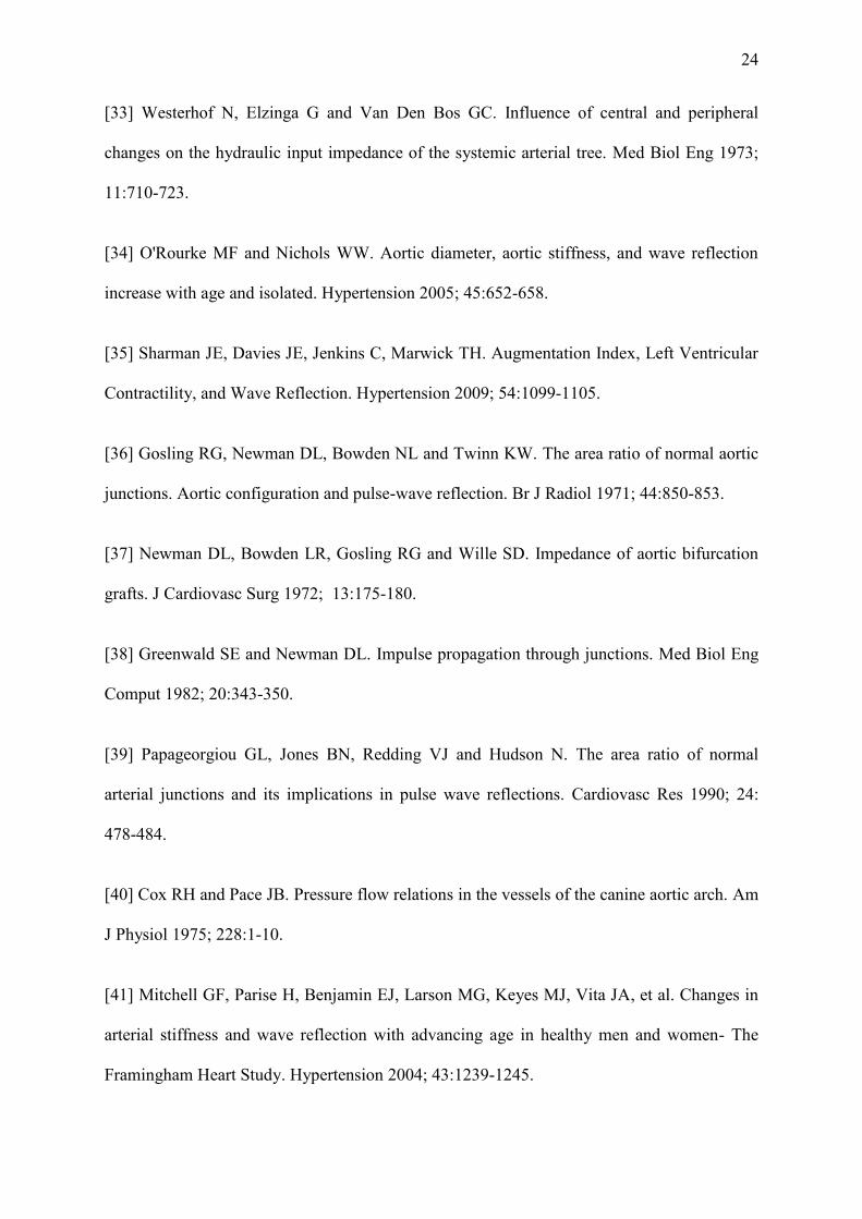
There is a significant difference in the morphology of the PU and PeU loops in all cases.

The PU-loop is a distinct loop with large hysteresis between the systolic and diastolic

portions of the curve. The PeU-loop exhibits much less hysteresis and in many cases, such as

the control conditions shown in Figure 1, the loop collapsed almost completely to a single

curve. In all cases, the early systolic portion of the loop was linear enabling a measurement of

the wave speed from the slope. In every condition the wave speed determined from the PU-

loop, c, was greater than the wave speed determined from the PeU-loop, ce, and all of the

differences were statistically significant. The values of c and ce and their ratio are reported for

all conditions in Table 2. We see that c during the thoracic occlusion is significantly higher

than control conditions (9.9±2.5 m/s vs. 6.0±2.6 m/s, p<0.05). ce calculated during the

thoracic occlusion was not statistically different from control. There were no significant

differences between either c or ce during any of the other occlusions compared to control

conditions.

B. Wave intensity and reflection index

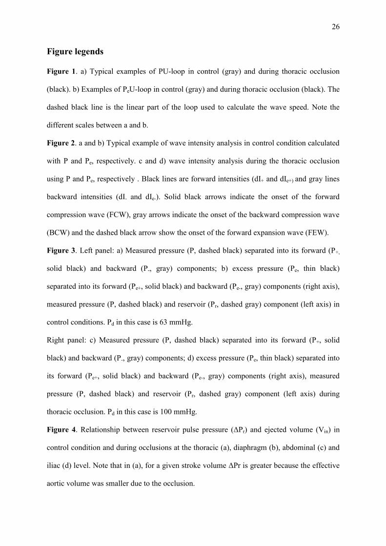
As seen in Figure 2, there were both similarities and differences between the wave

intensity calculated with P, dI = dPdU, and with Pe, dIe = dPedU. In all cases, the forward

wave intensities, dI+ and dIe+, were similar in shape with large peaks at the start (FCW) and

end (FEW) of systole. As discussed below, the morphology of these peaks was unchanged,

but there were differences in their magnitudes. However, the backward wave intensities, dI-

and dIe-, showed large differences with the no peaks discernible in the dIe- waveforms for

many of the cases. The magnitude of the three main wave intensity peaks, dIFCW, dIFEW,

dIBCW, dIeFCW, dIeFEW and dIeBCW and their ratios are reported in Table 2. For both of the

forward waves, FCW and FEW, dI > dIe and the difference is statistically significant in all

12

cases except for the thoracic and diaphragm occlusions for the FEW wave. The results for the

BCW are qualitatively different from the results for the forward waves. In all cases dIe << dI

with the differences being highly significant statistically. The reflection index, which is

related to the effective reflection coefficient, shows a similar pattern. For control conditions

the difference between RI and RIe is large and statistically significant, as reported in Table 2.

The times of the forward and backward peak intensities and the times of the onset of

the BCW and FEW when calculated using the wave-only and the reservoir-wave models are

reported in Table 3. As can be seen from the table, there is no significant difference in timing

between the two analyses in all conditions apart from the time of the onset of the FEW that

comes earlier when the analysis is performed with Pe, both in control and during the four

occlusions.

A comparison of wave intensities and reflection indices between occlusion and

control conditions yielded a broadly similar pattern. For both the FCW and the FEW there is

a slight but statistically significant decrease in the peak values of dI when the occlusion is in

the thoracic and diaphragm position and no significant differences when the occlusion is in

the more distal locations. This is true for the wave intensity calculated using the measured

pressure dI or the excess pressure dIe. For the BCW there is a large and highly significant

increase in the dI for the thoracic occlusion, an even larger increase for the diaphragm

occlusion and no significant difference for the abdominal and iliac occlusions. Although dIe

is significantly smaller than dI for all of the cases, this pattern persists for dIe; a significant

increase for the thoracic occlusion, an even larger increase for the diaphragm occlusion and

no differences for the two more distal occlusions.

The reflection index shows this pattern more clearly. For the reflection index

calculated using P, RI is more than double for the thoracic occlusion, more than triple for the

diaphragm occlusion and is not significantly different from control conditions for the

13

abdominal and iliac occlusions (Table 2). The reflection index calculated using the Pe, RIe, is

significantly smaller than the correspondent RI, but follows the same pattern; a large increase

for the thoracic occlusion, an even larger increase for the diaphragm occlusion and no

significant difference from control conditions for the two more distal occlusions.

C. Reservoir and excess pressure

P, Pr and Pe in the ascending aorta for a typical case are shown in Figure 3. As seen in

the figure, the aortic pressure increased significantly when the occlusion was in the thoracic

aorta. The averaged values of measured, reservoir and excess pulse pressures (ΔP, ΔPr and

ΔPe, respectively) and diastolic pressure Pd for all conditions are reported in Table 1. As can

be seen from the table, ΔP and ΔPr are significantly higher during thoracic occlusion

compared to the control, while ΔPe does not change significantly compared to the control

state for all the other occlusion conditions.

Figure 4 shows the relationship between the reservoir pulse pressure (ΔPr) and the

stroke volume (Vin) in control condition and during the occlusions for each dog. The Pearson

correlation factors between these two parameters were 0.70, 0.83, 0.87, 0.70, 0.72 in control

and during thoracic, diaphragm, abdominal and iliac occlusion (p<0.05 in all conditions). The

slope of the linear regression is higher for the thoracic occlusion than control, even higher for

the diaphragm occlusion but not significantly different from control for the abdominal and

iliac occlusions. A similar relationship is also found between pulse pressure and stroke

volume (correlation factors were 0.76, 0.85, 0.87, 0.78, 0.74 for control and occlusions,

p<0.05 in all conditions).

16

Another finding, common to the two methods, is that the averaged values of RI during

diaphragm occlusions are slightly higher than during the thoracic occlusion (Table 2) and in

some dogs reflections due to the diaphragm occlusion are bigger than these due to the

thoracic occlusion. A possible explanation of our result is that during this proximal occlusion

the aortic arch branches (subclavian and brachiocephalic arteries) play a greater role than

during the diaphragm occlusion. Westerhof et al. [33] previously suggested that the behaviour

of the aorta clamped at the diaphragm level is more similar to a uniform tube with a closed

end compared to the aorta occluded at a more proximal location, such as the thoracic level.

The authors explained this finding by considering the uniform tube when clamped proximally

as “short-circuited” because of the considerable role of the cephalic vessels and collaterals in

this condition.

The reflected waves have been used clinically/physiologically as a marker of arterial

stiffness [34] , thought to play a major role in the shape of the pressure waveform and in the

determination of the augmentation index (AIx); a correlate of mortality. However, recent

studies questioned the size and role of reflected waves. Sharman et al., [35] found a disparity

between the traditional explanation for the shape of the pressure waveform, due to reflected

waves, and the reservoir-wave approach. The authors suggested the role of the reflected

waves in the determination of AIx may have previously overstated. Davies et al., [24]

demonstrated that arterial reservoir increases with age and it is a major determinant of aortic

AIx, which they found not to be predominantly a measure of wave reflection. The authors

concluded that aortic pressure waveform is more related to the reservoir function than wave

reflection. Tyberg et al., reported the magnitude of the peak reflected pressure wave when

using the reservoir-wave model is ~ 6% of total pressure, where it would be ~30% of total

pressure using the wave-only model [21]. Our results agree with the above studies, and the

decrease of the backward compression wave intensity calculated using Pe is one of the most

17

significant results of this study. Similar results about the reduction of backward compression

waves using the reservoir-wave model compared to the wave-only model have been recently

reported by Mynard et al., [25]. The authors performed WIA in computational and animal

data and found lower values of backward compression waves and reflection coefficient when

the reservoir-wave system was applied compared to the traditional WIA. These results are in

line with our findings. However, they also found bigger backward expansion waves using the

reservoir-wave approach that were not present in our work.

Despite the reduction in the magnitude, dIeBCW and dIBCW showed a similar pattern

with significant reflections during the more proximal and no reflections from the more distal

occlusion. The small magnitude of the backward travelling waves found using the reservoir-

wave model can be explained if we consider that the arterial system is well-matched in the

forward but not in the backward direction [36,37,38,39]. We calculated the reflection

coefficients from the trifurcation of the aortic arch in forward direction as

3210

3210

YYYY

YYYYR

(10)

and for the backward direction as

3210

0213

YYYY

YYYYR

(11)

where Y0, Y1, Y2, Y3, are the characteristic admittances (Y=1/Z=A/ρc) for the ascending

aorta, brachiocefalic artery, left subclavian artery, and descending aorta, respectively. These

values were calculated using the characteristic impedances for the different vessels reported

by Cox and Pace [40] in anesthetized dogs in control condition, in which values of vascular

impedance have been calculated by averaging between 8 and 15 Hz. We found that the

reflection coefficient is 0.02 in the forward direction and -0.48 in the backward direction.

This means that approximately half of the energy carried by a backward wave in the thoracic

aorta will be reflected at the aortic arch. This may be the main reason for the observation of

18

small backward waves at the aortic root, even during the occlusion, using the reservoir-wave

model.

The pulse of the reservoir pressure is strongly related to the stroke volume as shown

in Figure 4. In particular, a different linear relationship can be observed during occlusion of

the aorta at the thoracic and diaphragm level compared to the control for Pr and Pe, caused by

the different pulse pressure in these conditions.

Davies et al. [24] studied the contribution of Pr and Pe in humans in relation with age.

They found that the contribution of the reservoir pressure to the increase of AIx with age is

larger than that of the reflected wave contribution as previously thought [41,42]; the increase

is largely due to the decrease of the aorta compliance and other elastic vessels. Our results are

related to their findings since the increase of pulse pressure due to the thoracic occlusion can

be compared to the increase of pressure due to age or to cardiovascular diseases such as

hypertension. Our findings confirm that the reservoir pressure makes a larger contribution to

the pressure waveform than the excess pressure, shown in Table 1, as previously reported by

other authors [24,43].

Conclusion

The reservoir-wave and the wave-only models produce similar WIA curves, although the

magnitudes are strikingly different. Both models lead to the conclusion that aortic occlusions

downstream the diaphragm level have little or no effect on hemodynamics in the ascending

aorta. The models yield different values of wave speed and different wave magnitudes,

despite using the same analytical techniques of the pressure-velocity loop and WIA. The

reservoir-wave model always yields lower values for all hemodynamic parameters studied.

The small magnitude of BCW in the aortic root during occlusions, using the reservoir-wave

model, could be explained by considering the geometry of the aortic arch which has different

magnitude of reflection coefficients in the forward and backward directions, although this

19

requires a larger study to confirm this observation. The differences found between the results

of wave speed and WIA based on the measured pressure and the reservoir/excess pressures

do not mean that the values based on excess pressure are erroneous. In the absence of other

independent techniques or evidence it is not currently possible to decide which of the two

models compared in this work is more correct.

20

References

[1] Parker KH. A brief history of arterial wave mechanics. Med Biol Eng Comput 2009;

47:111-118.

[2] Hamilton WF and Dow P. An experimental study of the standing waves in the pulse

propagated through the aorta. American Journal of Physiology 1938; 125: 48-59.

[3] Taylor MG. Wave Transmission through an Assembly of Randomly Branching Elastic

Tubes. Biophysical Journal 1966; 6: 697-716.

[4] Nichols WW and McDonald DA. Wave-velocity in the proximal aorta. Med & biol.

Engng 1972; 10: 327-335.

[5] Sagawa K, Lie RK and Schaefer J. Translation of Otto frank's paper “Die Grundform des

arteriellen Pulses” zeitschrift für biologie 37: 483–526 (1899). J.Mol.Cell.Cardiol 1990; 22:

253-254.

[6] Belz GG. Elastic properties and Windkessel function of the human aorta.

Cardiovasc.Drugs Ther 1995; 9:73-83.

[7] Westerhof N, Lankhaar J and Westerhof BE. The arterial windkessel. Med Biol Eng

Comput 2009; 47:131-141.

[8] Westerhof N, Bosman F, De Vries CJ and Noordergraaf A. Analog studies of the human

systemic arterial tree. J Biomech 1969; 2:121-134,IN1,135-136,IN3,137-138,IN5,139-143.

[9] Westerhof N, Elzinga G and Sipkema P. An artificial arterial system for pumping hearts.

J.Appl.Physiol 1971; 31:776-781.

21

[10] Parker KH, Jones CJH, Dawson JR and Gibson DG. What stops the flow of blood from

the heart? Heart Vessels 1988; 4: 241-245.

[11] Parker KH and Jones CJH. Forward and backward running waves in the arteries:

Analysis using the method of characteristics. J Biomech Eng 1990; 112:322-326.

[12] Hughes AD and Parker KH. Forward and backward waves in the arterial system:

impedance or wave intensity analysis? Med Biol Eng Comput 2009; 47:207-210.

[13] Avolio A, Westerhof BE, Siebes M and Tyberg JV. Arterial hemodynamics and wave

analysis in the frequency and time domains: an evaluation of the paradigms. Med Biol Eng

Comput 2009; 47:107-110.

[14] Khir AW and Parker KH. Wave intensity in the ascending aorta: Effects of arterial

occlusion. J Biomech 2005; 38:647-655.

[15] Zambanini A, Cunningham SL, Parker KH, Khir AW, Thom SAM and Hughes AD.

Wave-energy patterns in carotid, brachial, and radial arteries: A noninvasive approach using

wave-intensity analysis. Am J Physiol Heart Circ Physiol 2005; 289: H270-H276.

[16] Borlotti A, Khir AW, Rietzschel ER, De Buyzere ML, Vermeersch S, and Segers P.

Non-invasive determination of local pulse wave velocity and wave intensity: changes with

age and gender in the carotid and femoral arteries of healthy human. J Appl Physiol 2012;

113:727-735.

[17] Wang JJ, O'Brien AB, Shrive NG, Parker KH and Tyberg JV. Time-domain

representation of ventricular-arterial coupling as a windkessel and wave system. Am J

Physiol Heart Circ Physiol 2003; 284:H1358-H1368.

22

[18] Wang JJ, Flewitt JA, Shrive NG, Parker KH and Tyberg JV. Systemic venous

circulation. Waves propagating on a windkessel: Relation of arterial and venous windkessels

to systemic vascular resistance. Am J Physiol Heart Circ Physiol 2006; 290:H154-H162.

[19] Aguado-Sierra J, Alastruey J, Wang JJ, Hadjiloizou N, Davies J and Parker KH.

Separation of the reservoir and wave pressure and velocity from measurements at an arbitrary

location in arteries. Proc Inst Mech Eng Part H J Eng Med 2008; 222:403-416.

[20] Davies JE, Hadjiloizou N, Leibovich D, Malaweera A, Alastruey-Arimon J, Whinnett

ZI, et al. Importance of the aortic reservoir in determining the shape of the arterial pressure

waveform - The forgotten lessons of Frank. Artery Res 2007; 1:40-45.

[21] Tyberg JV, Davies JE, Wang Z, Whitelaw WA, Flewitt JA, Shrive NG, et al. Wave

intensity analysis and the development of the reservoir-wave approach. Med Biol Eng

Comput 2009; 47:221-232.

[22] Ochi H, Shimada T, Ikuma I, Morioka S and Moriyama K. Effect of a decrease in aortic

compliance on the isovolumic relaxation period of the left ventricle in man. Am J

Noninvasive Cardiol 1991; 5:149-154.

[23] Watanabe H, Ohtsuka S, Kakihana M and Sugishita Y. Coronary circulation in dogs

with an experimental decrease in aortic compliance. J Am Coll Cardiol 1993; 21:1497-1506.

[24] Davies JE, Baksi J, Francis DP, Hadjiloizou N, Whinnett ZI, Manisty CH, et al. The

arterial reservoir pressure increases with aging and is the major determinant of the aortic

augmentation index. Am J Physiol Heart Circ Physiol 2010; 298:H580-H586.

23

[25] Mynard JP, Penny DJ, Davidson MR and Smolich JJ. The reservoir-wave paradigm

introduces error into arterial wave analysis: a computer modelling and in-vivo study. J

Hypertens 2012; 30:734-743.

[26] Segers P, Swillens A, Vermeersch S. Reservations on the reservoir. J Hypertens 2012;

30:676-678.

[27] Wang JJ, Shrive NG, Parker KH, Hughes, AD and Tyberg JV. Wave propagation and

reflection in the canine aorta: analysis using a reservoir–wave approach. Can J Cardiol 2011;

27:389.e1-389.e10.

[28] Parker KH, Alastruey J and Stan G. Arterial reservoir-excess pressure and ventricular

work. Med Biol Eng Comput 2012; 50:419-424.

[29] Khir AW, O'Brien A, Gibbs JSR and Parker KH. Determination of wave speed and wave

separation in the arteries. J Biomech 2001; 34:1145-1155.

[30] Westerhof N, Sipkema P , Van Den Bos GC, and Elzinga G. Forward and backward

waves in the arterial system. Cardiovasc Res 1972; 6648-656.

[31] Van Den Bos GC, Westerhof N, Elzinga G and Sipkema P. Reflection in the systemic

arterial system: effects of aortic and carotid occlusion. Cardiovasc Res 1976; 10:565-573.

[32] Swalen MJP and Khir AW. Resolving the time lag between pressure and flow for the

determination of local wave speed in elastic tubes and arteries. J Biomech 2009; 42: 1574-

1577.

24

[33] Westerhof N, Elzinga G and Van Den Bos GC. Influence of central and peripheral

changes on the hydraulic input impedance of the systemic arterial tree. Med Biol Eng 1973;

11:710-723.

[34] O'Rourke MF and Nichols WW. Aortic diameter, aortic stiffness, and wave reflection

increase with age and isolated. Hypertension 2005; 45:652-658.

[35] Sharman JE, Davies JE, Jenkins C, Marwick TH. Augmentation Index, Left Ventricular

Contractility, and Wave Reflection. Hypertension 2009; 54:1099-1105.

[36] Gosling RG, Newman DL, Bowden NL and Twinn KW. The area ratio of normal aortic

junctions. Aortic configuration and pulse-wave reflection. Br J Radiol 1971; 44:850-853.

[37] Newman DL, Bowden LR, Gosling RG and Wille SD. Impedance of aortic bifurcation

grafts. J Cardiovasc Surg 1972; 13:175-180.

[38] Greenwald SE and Newman DL. Impulse propagation through junctions. Med Biol Eng

Comput 1982; 20:343-350.

[39] Papageorgiou GL, Jones BN, Redding VJ and Hudson N. The area ratio of normal

arterial junctions and its implications in pulse wave reflections. Cardiovasc Res 1990; 24:

478-484.

[40] Cox RH and Pace JB. Pressure flow relations in the vessels of the canine aortic arch. Am

J Physiol 1975; 228:1-10.

[41] Mitchell GF, Parise H, Benjamin EJ, Larson MG, Keyes MJ, Vita JA, et al. Changes in

arterial stiffness and wave reflection with advancing age in healthy men and women- The

Framingham Heart Study. Hypertension 2004; 43:1239-1245.

25

[42] Weber T, Auer J, O’Rourke MF, Kvas E, Lassnig E, Berent R, et al. Arterial stiffness,

wave reflections, and the risk of coronary artery disease. Circulation 2004; 109:184-189.

[43] Vermeersch SJ, Rietzschel ER, De Buyzere ML, Van Bortel LM, Gillibert TC, Verdonk

PR and Segers P. The reservoir pressure concept: the 3-element windkessel model revisited?

Application to the Asklepios population study. J Eng Math 2009; 64:417-428.

26

Figure legends

Figure 1. a) Typical examples of PU-loop in control (gray) and during thoracic occlusion

(black). b) Examples of PeU-loop in control (gray) and during thoracic occlusion (black). The

dashed black line is the linear part of the loop used to calculate the wave speed. Note the

different scales between a and b.

Figure 2. a and b) Typical example of wave intensity analysis in control condition calculated

with P and Pe, respectively. c and d) wave intensity analysis during the thoracic occlusion

using P and Pe, respectively . Black lines are forward intensities (dI+ and dIe+) and gray lines

backward intensities (dI- and dIe-). Solid black arrows indicate the onset of the forward

compression wave (FCW), gray arrows indicate the onset of the backward compression wave

(BCW) and the dashed black arrow show the onset of the forward expansion wave (FEW).

Figure 3. Left panel: a) Measured pressure (P, dashed black) separated into its forward (P+,

solid black) and backward (P-, gray) components; b) excess pressure (Pe, thin black)

separated into its forward (Pe+, solid black) and backward (Pe-, gray) components (right axis),

measured pressure (P, dashed black) and reservoir (Pr, dashed gray) component (left axis) in

control conditions. Pd in this case is 63 mmHg.

Right panel: c) Measured pressure (P, dashed black) separated into its forward (P+, solid

black) and backward (P-, gray) components; d) excess pressure (Pe, thin black) separated into

its forward (Pe+, solid black) and backward (Pe-, gray) components (right axis), measured

pressure (P, dashed black) and reservoir (Pr, dashed gray) component (left axis) during

thoracic occlusion. Pd in this case is 100 mmHg.

Figure 4. Relationship between reservoir pulse pressure (ΔPr) and ejected volume (Vin) in

control condition and during occlusions at the thoracic (a), diaphragm (b), abdominal (c) and

iliac (d) level. Note that in (a), for a given stroke volume ΔPr is greater because the effective

aortic volume was smaller due to the occlusion.

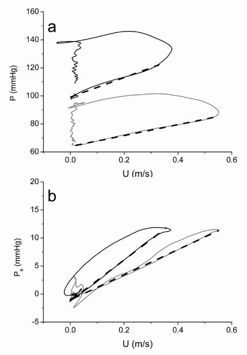
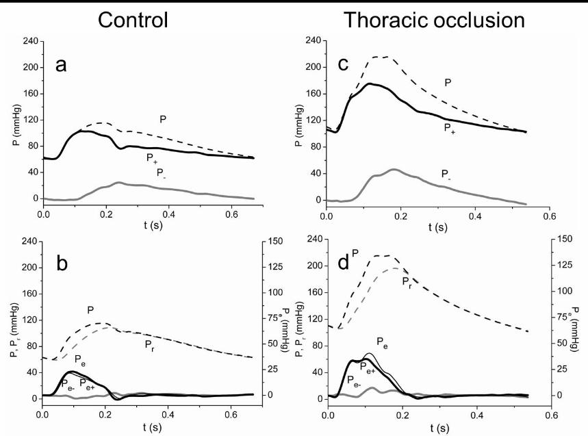
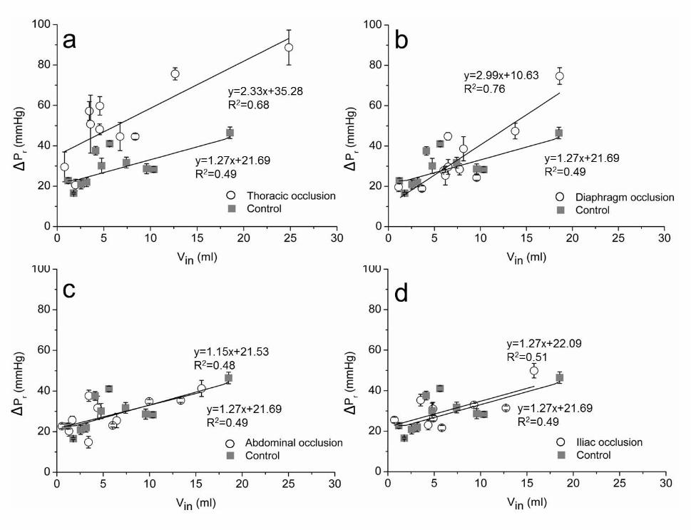
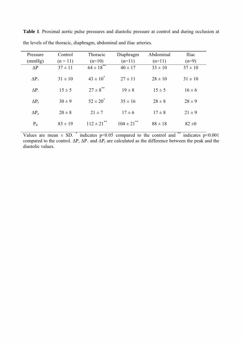
Table 1. Proximal aortic pulse pressures and diastolic pressure at control and during occlusion at

the levels of the thoracic, diaphragm, abdominal and iliac arteries.

Pressure (mmHg)

Control (n = 11)

Thoracic (n=10)

Diaphragm (n=11)

Abdominal (n=11)

Iliac (n=9)

ΔP 37 ± 11 64 ± 18** 40 ± 17 33 ± 10 37 ± 10

ΔP+ 31 ± 10 43 ± 10* 27 ± 11 28 ± 10 31 ± 10

ΔP- 15 ± 5 27 ± 8** 19 ± 8 15 ± 5 16 ± 6

ΔPr 30 ± 9 52 ± 20* 35 ± 16 28 ± 8 28 ± 9

ΔPe 20 ± 8 21 ± 7 17 ± 6 17 ± 8 21 ± 9

Pd 83 ± 19 112 ± 21** 104 ± 21** 88 ± 18 82 ±0

Values are mean ± SD. * indicates p<0.05 compared to the control and ** indicates p<0.001 compared to the control. ΔP, ΔP+ and ΔPr are calculated as the difference between the peak and the diastolic values.

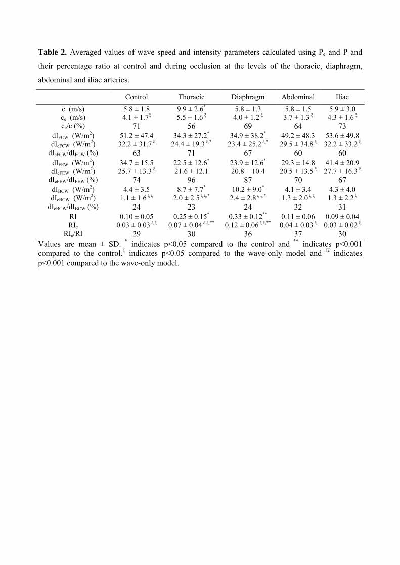
Table 2. Averaged values of wave speed and intensity parameters calculated using Pe and P and

their percentage ratio at control and during occlusion at the levels of the thoracic, diaphragm,

abdominal and iliac arteries.

Control Thoracic Diaphragm Abdominal Iliac

c (m/s) ce (m/s) ce/c (%)

5.8 ± 1.8 4.1 ± 1.7ξ

71

9.9 ± 2.6*

5.5 ± 1.6 ξ 56

5.8 ± 1.34.0 ± 1.2 ξ

69

5.8 ± 1.5 3.7 ± 1.3 ξ

64

5.9 ± 3.04.3 ± 1.6 ξ

73 dIFCW (W/m2) dIeFCW (W/m2)

dIeFCW/dIFCW (%)

51.2 ± 47.4

32.2 ± 31.7 ξ 63

34.3 ± 27.2*

24.4 ± 19.3 ξ,* 71

34.9 ± 38.2*

23.4 ± 25.2 ξ,* 67

49.2 ± 48.3 29.5 ± 34.8 ξ

60

53.6 ± 49.832.2 ± 33.2 ξ

60 dIFEW (W/m2) dIeFEW (W/m2)

dIeFEW/dIFEW (%)

34.7 ± 15.5 25.7 ± 13.3 ξ

74

22.5 ± 12.6*

21.6 ± 12.1 96

23.9 ± 12.6*

20.8 ± 10.4 87

29.3 ± 14.8 20.5 ± 13.5 ξ

70

41.4 ± 20.927.7 ± 16.3 ξ

67 dIBCW (W/m2) dIeBCW (W/m2)

dIeBCW/dIBCW (%)

4.4 ± 3.5 1.1 ± 1.6 ξ ξ

24

8.7 ± 7.7*

2.0 ± 2.5 ξ ξ,* 23

10.2 ± 9.0*

2.4 ± 2.8 ξ ξ,* 24

4.1 ± 3.4 1.3 ± 2.0 ξ ξ

32

4.3 ± 4.01.3 ± 2.2 ξ

31 RI RIe

RIe/RI

0.10 ± 0.05 0.03 ± 0.03 ξ ξ

29

0.25 ± 0.15*

0.07 ± 0.04 ξ ξ,** 30

0.33 ± 0.12**

0.12 ± 0.06 ξ ξ,** 36

0.11 ± 0.06 0.04 ± 0.03 ξ

37

0.09 ± 0.040.03 ± 0.02 ξ

30 Values are mean ± SD. * indicates p<0.05 compared to the control and ** indicates p<0.001 compared to the control.ξ indicates p<0.05 compared to the wave-only model and ξξ indicates p<0.001 compared to the wave-only model.

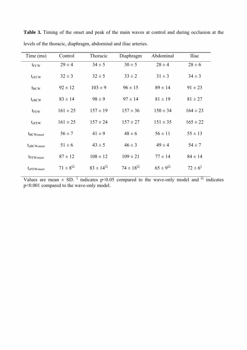
Table 3. Timing of the onset and peak of the main waves at control and during occlusion at the

levels of the thoracic, diaphragm, abdominal and iliac arteries.

Time (ms) Control Thoracic Diaphragm Abdominal Iliac

tFCW 29 ± 4 34 ± 5 30 ± 5 28 ± 4 28 ± 6

teFCW 32 ± 3 32 ± 5 33 ± 2 31 ± 3 34 ± 3

tBCW 92 ± 12 103 ± 9 96 ± 15 89 ± 14 91 ± 23

teBCW 83 ± 14 98 ± 9 97 ± 14 81 ± 19 81 ± 27

tFEW 161 ± 25 157 ± 19 157 ± 36 150 ± 34 164 ± 23

teFEW 161 ± 25 157 ± 24 157 ± 27 151 ± 35 165 ± 22

tBCWonset 56 ± 7 41 ± 9 48 ± 6 56 ± 11 55 ± 13

teBCWonset 51 ± 6 43 ± 5 46 ± 3 49 ± 4 54 ± 7

tFEWonset 87 ± 12 108 ± 12 109 ± 21 77 ± 14 84 ± 14

teFEWonset 71 ± 8ξξ 83 ± 14ξξ 74 ± 18ξξ 65 ± 9ξξ 72 ± 6ξ

Values are mean ± SD. ξ indicates p<0.05 compared to the wave-only model and ξξ indicates p<0.001 compared to the wave-only model.