Researcher 2018;10(5) ...

Researcher 2018;10(5) http://www.sciencepub.net/researcher

89

Beta-Binomial Mixture Models: Its Consistent And Efficient Performance Over Binomial Model.

1*Akomol Afe. A. A., 1maradesa. A. And 2yussuf T. O

1 Department Of Statistics, Federal University Of Technology, Akure, Nigeria Corresponding [email protected], [email protected]

2national Institute For Educational Planning And Administration, Ondo [email protected]

Abstract: Beta binomial Model is a standard choice for modeling multiple sequences of binary responses. This research was carried out based on the efficiency and consistency of Beta-binomial Model (BBM) in tracking and forecasting purchasing pattern of consumers of Soft drink using secondary data collected from whole sales outlet of a standard bottling Company, The model (BBM) as compared to binomial model (BM) was fitted to the data.

Akaike Criterion, Bayesian Criterion and goodness of fit were used to establish the efficiency and flexibility of BBM over BM in predicting the customers’ purchasing pattern. The analysis shows that Beta-Binomial Model fitted better coupled with it low standard error in predicting future purchasing when compared with Binomial Model. We can therefore say that the predictive efficiency of this model is high. The usefulness of BBM as illustrated using real data depicts that it can be relied on for consistent planning and decision making. [ Akomol Afe. A. A., maradesa. A. And yussuf T. O. Beta-Binomial Mixture Models: Its Consistent And Efficient Performance Over Binomial Model. Researcher 2018;10(5):89-97]. ISSN 1553-9865 (print); ISSN 2163-8950 (online). http://www.sciencepub.net/researcher. 12. doi:10.7537/marsrsj100518.12. Key words: Beta-binomial model, Predictive Beta-binomial Model, Akaike Information Criteria (AIC), Bayesian Information Criteria (BIC), Coefficient of variation

1 Introduction

Generating accurate, valid and reliable consumer behavioral pattern is very crucial to the producers of economics products. In fact, many renowned economics had studied how consumers react to increase in price of a certain commodity; this has laid a solid foundation for the law of demand and supply which state that the higher the price the lower the quantity demanded and vice versa. To study the consumer buying behavior, it therefore becomes imperative to the producers and the economy planner to track their behavior as regards their product, for future planning, and optimum profitability. This can be modeled using a beta-binomial distribution, if the probability of success parameter, p, of a Binomial distribution has a beta distribution with shape parameters α > 0 and β > 0, the resulting distribution is known as a beta binomial distribution. For a binomial distribution, p is assumed to be fixed for successive trials or periods. For the beta-binomial distribution, the value of p changes for each trial or period and it is said to be random variable having a beta-binomial distribution. Many researchers have contributed to the theory of beta binomial distribution and its applications in various fields, among them are Akomolafe et al (2009), Pearson (1925), Skellam (1948), Lord (1965), Greene (1970), Massy et. al. (1970), Griffiths (1973), Williams (1975), Huynh (1979), Wilcox (1979), Smith (1983), Lee and Sabavala (1987), Hughes and Madden (1993), and

Shuckers (2003), are notable. Since study consumer behavior is very important to the business men and entrepreneurs around the world, because it determines to a great extents the going concern of their company, capacity of production and their net and capital investment as well as their total profit, then this project discusses the efficiency of the beta-binomial model as compared to the traditional binomial model in forecasting the consumer buying behavioral pattern; a case study of Seven up Bottling Company Plc (Ibadan Depot), and its application in predicting the future consumers of beverages. Beta-Binomial Model is being employed in this study because of its capability of capturing buying behavior pattern of consumers. The computed predictions are also compared for the four products under investigation so as to determine the efficiency of beta-binomial model compared to the conventional binomial model at different proposed production volume. The coefficient of variation at different sales volume showed the efficiency with respect to the lower relative standard deviation. It is hoped that the finding of this paper will be useful for practitioners in various fields, most especially the researchers and various economics planner such as market researchers, and business administrators. 1.1 Source Of The Data

The result reported in this research work is based on secondary data available from wholesales standard outlets of beverages outfit for two years. These reports


90

have been generated with the help of sales record (purchase data), precisely Seven up Bottling Company Plc, available in the outlet which showcases the identity of customers as they patronize the outlets and eventually buy the products in large quantity. 2 Derivation Of Mean, Variance And Posterior Predictive Mean

The binomial model is P (x) = nCxPnqn – x

For O≤ P≤ 1, where x is a random variable. Now, suppose p of binomial distribution varies

from trial to trial and follow beta distribution. It is in this case, we can say beta distribution is a conjugate distribution of binomial distribution. Then this can be modeled using beta binomial model.

= Let P be represented by θ, then the beta distribution can be re-written as;

= (1) The mean and variance of this BBD can be therefore be obtained by the following expectation procedures. The

equation (1) above represent the beta-distribution when P of binomial varies from period to period.

=

Since ,

then= (2)

= (3)

= (4)

= (5)

E ( = (6) The mean of beta distribution is given in (2) above Since P = x/n, it can be written as

= x/n; x = n Taking the expectation of both sides

E (x)=E (n

E (x)=nE ( Mean: E (x)= n α/(α + β) (7) The mean of BBM is represented by equation (3) above Now, for the variance, we follow the same approach

Var =E 2 –[ (E )]2

= α – 1 (1 – θ) β – 1 dθ -

= α – 1 (1 – θ) β – 1 dθ - (8)

= α – 1 (1 – θ) β – 1 dθ - (9)

= (10)

= (11)

= (12)

= (13)


91

= (14)

= (15)

= (16)

= (17) The variance of beta distribution is represented by (17) above. To prove the variance of conditional

distribution, it follows that,

= (18)

Where x is a binomial variable and follows beta distribution

(19)

= (20)

= (21)

= (22)

Since =1, then we can say

= (23)

= (24)

= (25)

= (26)

= (27) Now,

= (28)

= = (30) Therefore, variance of beta binomial is given by (30) above, the posterior predictive mean can be obtained as

follows:

E ( ; x, n, α, β) = P ( ; x, n, α, β) d (31)

. (32)

= (33)

= (34)

= (35)


92

= (36)

= . (37)

= (38)

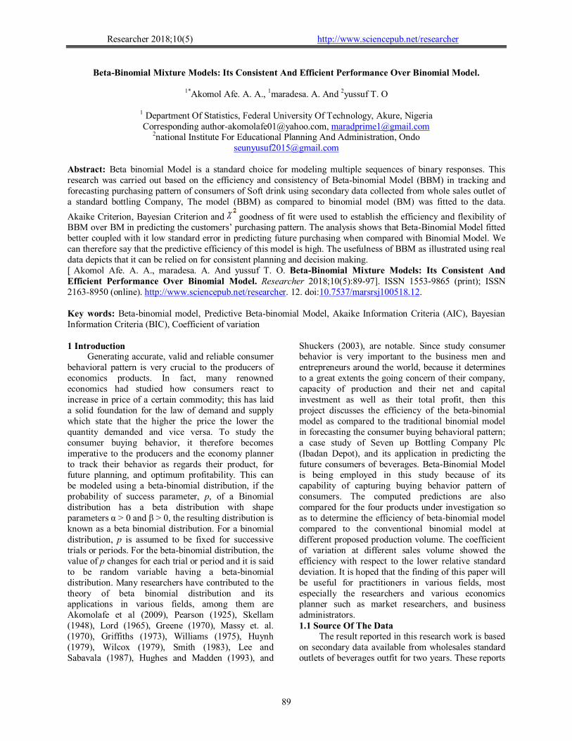
= + (39) The (39) above is the posterior predictive mean

of BBM To mix binomial distribution with beta

distribution: it is assumed that the data collected on purchased data from 7up Bottling Company follows binomial distribution and P denotes the probability that a purchase will be made and (1-P) when no purchase is made. When purchase of any of Pepsi, 7up, Teem and Mirinda is made, there arise a binomial with unvarying P. but if the probability that a purchase is made is changing from period to period, this can be modeled by an Hybrid Model called Beta-binomial Hybrid Distribution. The efficiency of this model in

tracking the pattern of purchase of consumers which result to determination of psychology of consumer’s behavior can thereafter be detected by getting the main behavioral pattern and attitude towards consuming the 7up, Pepsi, Teem and Mirinda. The implementation of the BBM was done by written simple r codes, and the parameter estimation based on principle of both method of moment and maximum likelihood with the developed codes. The necessary goodness of fit test was also done by the AIC and BIC generated through the method of maximum likelihood in the GAMLSS and VGAM R-library.

The beta distribution is given as and B (α, β)=

is a beta function Since θ = P is probability that purchase will be made and it varies from period to period, therefore the set of P

form random sample which follows beta distribution.

= (40)

= (41)

= (42)

From beta function: B (α, β)= , we can conclude that the BBD is expressed as shown below:

= (43) The equation (43) above is the beta-binomial model

3 Numerical Results And Discussion 3.1 Fitting BBM to Pepsi Flavor Table 1: Comparision Criteria for Binomial and Predictive Betabinomial Model Binomial (BM) Betabinomial (BBM) AIC 40.82 -61.13645 BIC 0.001 -70.1628

From the table1 above, it can be deduced that the

Predictive Beta-Binomial Model fits the Pepsi

purchase data reasonably well. AIC and BIC showed that Beta-binomial is better than Binomial Model in modeling the consumers’ preference for soft drinks. Therefore, BBM provides good fit regarding the prediction of future sales of the Pepsi and the model is efficient to describe the behavior of consumers. Since 2 calculated (25986.63)> 2 tabulated (12.592), we thereby have utmost statistical reason not to accept Ho,

and conclude that the goodness of fit is significant for BBM, and it therefore modeled the Pepsi data accurately and reasonably well.


93

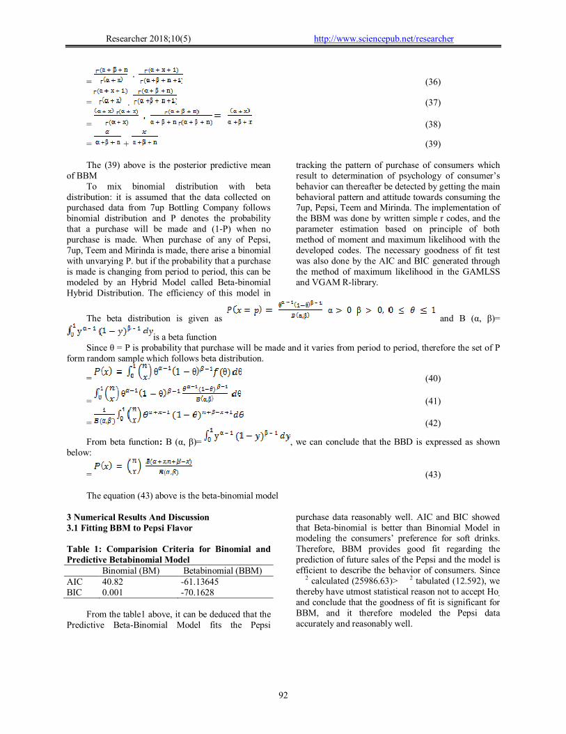
Table 2: Estimation of Parameters Parameter Binomial Model (BM) Betabinomial Model (BBM) P 0.5092 α 0.8144925 β 0.7850609

The parameter and determine the shape of the distribution. With these two parameters greater than zero, we have beta binomial distribution. Since probability of success, p =0.5092, of a Binomial

distribution has a beta distribution with shape

parameters > 0 and > 0, with this, the resulting distribution is known as a beta binomial distribution.

Table 3: Efficiency of BBM at Different Proposed Sales Volume of Pepsi Flavor Future sales (‘0000’)

Mean of BM

Mean of BBM

Standard Error of BM

Standard Error of BBM

CV (%) of BM

CV (%) of BBM

30 4.305429 15.276 1.453652 0.4255340 33.76324 2.7856377 40 4.823770 20.368 1.538670 0.4228329 31.89767 2.0759667 50 5.673684 25.460 1.668725 0.4212039 29.41167 1.6543752 60 6.674332 30.552 1.809907 0.4201144 27.11742 1.3750799 70 7.847269 35.644 1.962509 0.419334 25.00881 1.1764518 80 9.302026 40.736 2.136688 0.4187485 22.97013 0.9879570 90 11.362336 45.828 2.361490 0.4182922 20.78349 0.912739 100 15.655153 50.920 2.771922 0.4179269 17.70613 0.8207520

From the table 3 above, we can conclude that

coefficient of variation of BBM decreases with increasing in the sales volume (purchase). Although, the CV of BM is significantly larger than that of BBM, the BBM produces best estimate for predicting the probability of getting the future targeted sales for Pepsi. At volume 900,000crates, the CV is 0.9280664% and shows a decrease of 0.0935987% at volume 1,000,000 crates. The decrease in the CV of BBM is as a result that the model fitted the future sales the most as compared to its binomial counterpart, so

BBM is efficient at different future sale and it is very efficient at significantly higher sales. The average sale of Pepsi increase with increasing production volume, and at sales 1million crates the coefficient of variation for BM and BBM are 17.70613% and 0.8207520% respectively which reflect that the CV of BBM is significantly reduced at sales one million. The BBM stands to be the best model for Pepsi due to its lower coefficient of variation. 3.2 Fitting BBM for 7up flavor

Table 4: Estimation of model’s parameter Parameter Binomial Betabinomial P 0.4975977 α 0.8659094 β 0.8742703 2=41308.5

The parameter and determine the shape of the distribution. With these two parameters greater than zero, the resulting distribution is BBM. Since probability of success, p=0.5092, of a Binomial distribution has a beta distribution with shape

parameters > 0 and > 0, with this, the resulting distribution is known as a beta binomial distribution. 3.2.1 Comparison criteria for binomial and Predictive BBM

Since 2 calculated (41308.5) > 2 tabulated (12.592), we thereby have utmost statistical reason not

to accept Ho, and conclude that the goodness of fit is significant for BBM. BBM therefore modeled the 7up data reasonably well. The result obtained in BM cannot be totally relied upon in decision making as regarding consumers’ altitude to 7up Flavor. Also the AIC of -81.075 and 41.269 for BBM and BM respectively revealed that BBM provides consistent numerical evidence for predicting consumers’ habit regarding 7up.


94

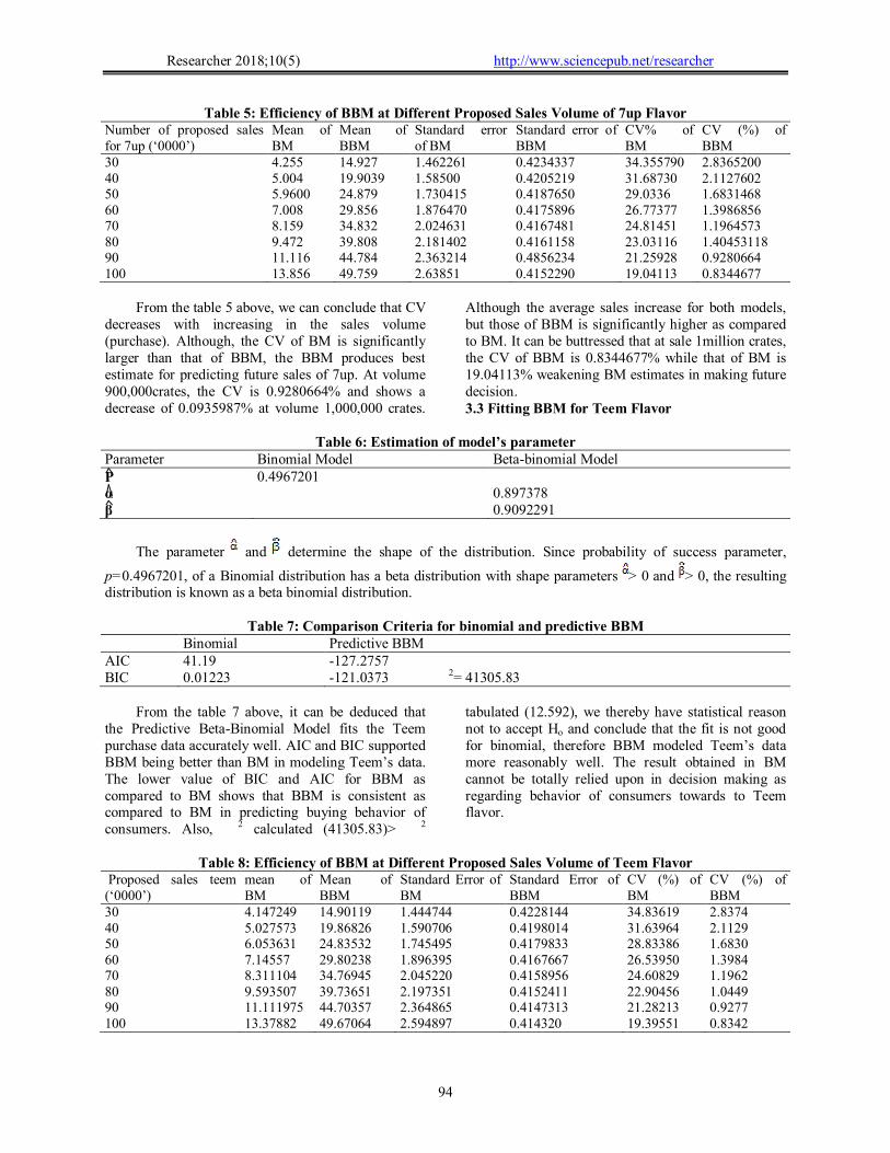
Table 5: Efficiency of BBM at Different Proposed Sales Volume of 7up Flavor Number of proposed sales for 7up (‘0000’)

Mean of BM

Mean of BBM

Standard error of BM

Standard error of BBM

CV% of BM

CV (%) of BBM

30 4.255 14.927 1.462261 0.4234337 34.355790 2.8365200 40 5.004 19.9039 1.58500 0.4205219 31.68730 2.1127602 50 5.9600 24.879 1.730415 0.4187650 29.0336 1.6831468 60 7.008 29.856 1.876470 0.4175896 26.77377 1.3986856 70 8.159 34.832 2.024631 0.4167481 24.81451 1.1964573 80 9.472 39.808 2.181402 0.4161158 23.03116 1.40453118 90 11.116 44.784 2.363214 0.4856234 21.25928 0.9280664 100 13.856 49.759 2.63851 0.4152290 19.04113 0.8344677

From the table 5 above, we can conclude that CV

decreases with increasing in the sales volume (purchase). Although, the CV of BM is significantly larger than that of BBM, the BBM produces best estimate for predicting future sales of 7up. At volume 900,000crates, the CV is 0.9280664% and shows a decrease of 0.0935987% at volume 1,000,000 crates.

Although the average sales increase for both models, but those of BBM is significantly higher as compared to BM. It can be buttressed that at sale 1million crates, the CV of BBM is 0.8344677% while that of BM is 19.04113% weakening BM estimates in making future decision. 3.3 Fitting BBM for Teem Flavor

Table 6: Estimation of model’s parameter

Parameter Binomial Model Beta-binomial Model P 0.4967201 α 0.897378 β 0.9092291

The parameter and determine the shape of the distribution. Since probability of success parameter,

p=0.4967201, of a Binomial distribution has a beta distribution with shape parameters > 0 and > 0, the resulting distribution is known as a beta binomial distribution.

Table 7: Comparison Criteria for binomial and predictive BBM

Binomial Predictive BBM AIC 41.19 -127.2757 BIC 0.01223 -121.0373 2= 41305.83

From the table 7 above, it can be deduced that

the Predictive Beta-Binomial Model fits the Teem purchase data accurately well. AIC and BIC supported BBM being better than BM in modeling Teem’s data. The lower value of BIC and AIC for BBM as compared to BM shows that BBM is consistent as compared to BM in predicting buying behavior of consumers. Also, 2 calculated (41305.83)> 2

tabulated (12.592), we thereby have statistical reason not to accept Ho and conclude that the fit is not good for binomial, therefore BBM modeled Teem’s data more reasonably well. The result obtained in BM cannot be totally relied upon in decision making as regarding behavior of consumers towards to Teem flavor.

Table 8: Efficiency of BBM at Different Proposed Sales Volume of Teem Flavor

Proposed sales teem (‘0000’)

mean of BM

Mean of BBM



CV (%) of BM

CV (%) of BBM

30 4.147249 14.90119 1.444744 0.4228144 34.83619 2.8374 40 5.027573 19.86826 1.590706 0.4198014 31.63964 2.1129 50 6.053631 24.83532 1.745495 0.4179833 28.83386 1.6830 60 7.14557 29.80238 1.896395 0.4167667 26.53950 1.3984 70 8.311104 34.76945 2.045220 0.4158956 24.60829 1.1962 80 9.593507 39.73651 2.197351 0.4152411 22.90456 1.0449 90 11.111975 44.70357 2.364865 0.4147313 21.28213 0.9277 100 13.37882 49.67064 2.594897 0.414320 19.39551 0.8342


95

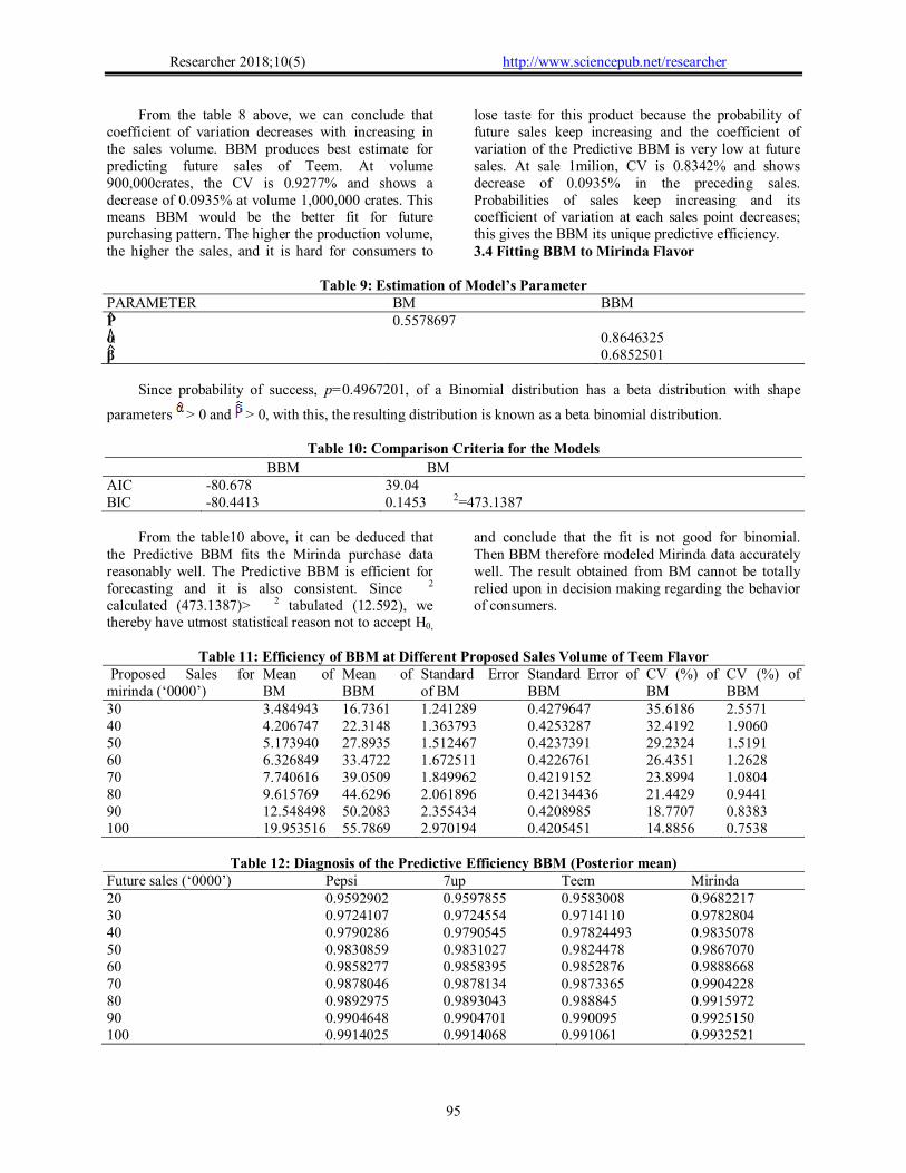
From the table 8 above, we can conclude that coefficient of variation decreases with increasing in the sales volume. BBM produces best estimate for predicting future sales of Teem. At volume 900,000crates, the CV is 0.9277% and shows a decrease of 0.0935% at volume 1,000,000 crates. This means BBM would be the better fit for future purchasing pattern. The higher the production volume, the higher the sales, and it is hard for consumers to

lose taste for this product because the probability of future sales keep increasing and the coefficient of variation of the Predictive BBM is very low at future sales. At sale 1milion, CV is 0.8342% and shows decrease of 0.0935% in the preceding sales. Probabilities of sales keep increasing and its coefficient of variation at each sales point decreases; this gives the BBM its unique predictive efficiency. 3.4 Fitting BBM to Mirinda Flavor

Table 9: Estimation of Model’s Parameter

PARAMETER BM BBM P 0.5578697 α 0.8646325 β 0.6852501

Since probability of success, p=0.4967201, of a Binomial distribution has a beta distribution with shape

parameters > 0 and > 0, with this, the resulting distribution is known as a beta binomial distribution.

Table 10: Comparison Criteria for the Models

BBM BM AIC -80.678 39.04 BIC -80.4413 0.1453 2=473.1387

From the table10 above, it can be deduced that

the Predictive BBM fits the Mirinda purchase data reasonably well. The Predictive BBM is efficient for forecasting and it is also consistent. Since 2 calculated (473.1387)> 2 tabulated (12.592), we thereby have utmost statistical reason not to accept H0,

and conclude that the fit is not good for binomial. Then BBM therefore modeled Mirinda data accurately well. The result obtained from BM cannot be totally relied upon in decision making regarding the behavior of consumers.

Table 11: Efficiency of BBM at Different Proposed Sales Volume of Teem Flavor

Proposed Sales for mirinda (‘0000’)

Mean of BM

Mean of BBM



CV (%) of BM

CV (%) of BBM

30 3.484943 16.7361 1.241289 0.4279647 35.6186 2.5571 40 4.206747 22.3148 1.363793 0.4253287 32.4192 1.9060 50 5.173940 27.8935 1.512467 0.4237391 29.2324 1.5191 60 6.326849 33.4722 1.672511 0.4226761 26.4351 1.2628 70 7.740616 39.0509 1.849962 0.4219152 23.8994 1.0804 80 9.615769 44.6296 2.061896 0.42134436 21.4429 0.9441 90 12.548498 50.2083 2.355434 0.4208985 18.7707 0.8383 100 19.953516 55.7869 2.970194 0.4205451 14.8856 0.7538

Table 12: Diagnosis of the Predictive Efficiency BBM (Posterior mean)

Future sales (‘0000’) Pepsi 7up Teem Mirinda 20 0.9592902 0.9597855 0.9583008 0.9682217 30 0.9724107 0.9724554 0.9714110 0.9782804 40 0.9790286 0.9790545 0.97824493 0.9835078 50 0.9830859 0.9831027 0.9824478 0.9867070 60 0.9858277 0.9858395 0.9852876 0.9888668 70 0.9878046 0.9878134 0.9873365 0.9904228 80 0.9892975 0.9893043 0.988845 0.9915972 90 0.9904648 0.9904701 0.990095 0.9925150 100 0.9914025 0.9914068 0.991061 0.9932521


96

From table 11 above, we can conclude that CV decreases with increasing in sales volume. Although, CV of BMl is significantly larger than of BBM, BBM produces best result for predicting future sales of Mirinda. At volume 900,000crates, the CV is 0.8383% and shows a decrease of 0.0845% at volume 1million-crates. It means BBM produces better estimate as compared to BM.

In general, BBM provides good fit for all the four flavors under investigation and its predictive efficiency can be relied upon in prospective planning. For this reason, it provides excellent evidence regarding the prediction made about the four flavors. It can be concluded BBM performed exceedingly better for Pepsi and Mirinda because the CV% of both Pepsi and Mirinda are lower than that of other two flavors.

The table 12 above shows that the probability of purchases increases as the production volume increases. For instances, if the production volume is 1million crate, then the probability that all the produced 1million-crates will be purchased can be modeled by the above predictive probabilities. It can then be deduced from the table above that out of one million-crates produced, the probability that all the 1million crates will be purchased are 0.9914025, 0.9914068, 0.991061 and 0.9932521 for pepsi,7up, Teem and Mirinda respectively. We now have statistical reason to say, as the production volume increases, the probability of purchase is tending to unity. The purchasing power of the consumer for the four flavors at production volume one million is 96.752417%. The populace is having good taste for the flavors and they are ready to buy all the produced flavors at any given period. That is, when production volume is sufficiently large say (N), so also the probability of purchasing all the products will be extremely large. From the predictive probabilities above, one can conclude that the probabilities of purchasing Mirinda product are higher as compared to other three products. Since there are no significant differences between all the predicted probabilities for all the flavors, then we can conclude that the four flavors, rolling out of 7up Bottling Company Plc, will continue to gain public acceptance of the populace of Ibadan because the products had met their taste and have been satisfying their refreshing taste for long period of time. Conclusion

The BBM provides a good basis for relying on the predicted values for adequate and consistent decision making and planning based on the study; BBM predicted that the probability of purchase increases with increase in the number of future sales. In general, BBM has stood the test of Akaike and Bayesian Information Criteria, for this reason, it

provides efficient, consistence and reliable evidence based on the prediction obtained from the analytical expressions about the four flavors. References 1. Akomolafe A. A and Amahia G. N, (2009).

Customer Behaviour Transaction Data Analysis, international journal of management. Volume 1 (1) p (32-37).

2. Akomolafe A. A, Awogbemi C. A, Alagbe S. A (2012). Counting Dropout Rate of consumers; A case study of durable goods, mathematical theory and modeling vol 2 p (6-11).

3. Akomolafe A. A. (2011). Analysis of consumers depth of Repeat purchasing pattern: An exploratory study of beverages Buying behavior data, journal of business and organizational development Vol 3, p (5-8).

4. Chandrabose M., Pushpa, W. and Roshan, D. (2013). The McDonald Generalized Beta-Binomial Distribution: A New Binomial Mixture Distribution and Simulation Based Comparison with Its Nested Distributions in Handling Over-dispersion. International Journal of Statistics and Probability, Vol2, p ( 213-223).

5. Nthiwa M. J, Ali I, Orawo L. (2014). Estimating Equation for estimation of Mc Donald Generalized Beta-binomial Parameter, Department of mathematics, Egerton University, Njoro, Kenya.

6. Brooks, R. J (1984). Approximate likelihood ratio tests in the Analysis of Beta Binomial data, Appl. Statist, Vol 33 p (285-289).

7. Alexandre D. and Maxim P. (2008). Performance of Binomial and Beta-binomial Models of demand forecasting for multiple slow-moving inventory items. Centre for industrial Engineering and Computer Sciences ( Ecole Nationale Superieure des mines de Saint-Etienne 158, Cours Fauriel, 42023 saint Etienne, France).

8. Chambers JM, Hastie TJ (eds.) (1992). Statistical Models in S. Chapman & Hall, London.

9. Cribari-Neto F, Lima LB (2007). “A Misspecification Test for Beta Regressions.” Technical report.

10. Cribari-Neto F, Zeileis A (2010). “Beta Regression in R.” Journal of Statistical Software, 34(2), 1–24. URL http://www.jstatsoft.org/v34/i02/.

11. Fader, P. S. and D. C. Schmittlein. (1993). Excess behavioral loyalty for high-share brands: Deviations from the Dirichlet model for repeat purchasing. J. Marketing Res. 30(4), 478-493.

12. Manohar U.K. and Alvin J.S. (1981). On the reliability and predictive validity of purchase intention measure pp (45-81).


97

13. Fernado A.O. and Wing K.T. (1996). Bayesian Estimation of Betabinomial Models by Simulating Posterior Densities, vol 13 p (43-56).

14. Paul S.R. (1884). Three parameters generalization of binomial distribution, Department of mathematics University of Windsor, Antario, Canada.

15. Hilbe, J.M and Robinson A.P. (2012). COUNT package, CRAN.

16. Hilbe, J.M. and Robinson A.P. (2013) msme package, CRAN.

17. Ram C.T, Ramesh C.G and John G. (1994).estimation of parameters in beta-binomial model v 46 p (317-331), the university of Texas San Antonio, TX 78249, USA.

18. Hill, R.M., (1999). Bayesian decision-making in inventory modeling. IMA Journal of Mathematics Applied in Business and Industry, vol10 p (165-176).

19. Berry. D, (1996). A Bayesian Perspective, Duxbury Press, New York.

20. Williams. D (1975), "The analysis of binary responses from toxicological experiments involving reproduction and teratogenicity", Biometrics 31, p (949-952).

21. Aaker, D.A. (1991), Managing Brand Equity. Capitalizing on the Value of Brand Name, the Free Press, and New York, NY.

22. Anderson, E.W., Fornell, C. and Lehmann, D. (1994), “Customer satisfaction, market share, and profitability: findings from Sweden”, Journal of Marketing, Vol. 58, July, p (53-66).

23. Skellam, I.G (1948). A probability distribution derived from the binomial distribution by regarding the probability of success as a variable between sets of trials, J. Roy statists’ p (257-261).

24. Mikis D.S., Robert R.A., (2007). Generalized Additive Models for Location Scale and Shape (Gamlss in R). Journal of statistical software v23 p (5-23).

5/25/2018

Researcher 2018;10(5) ...

Documents

Transcript of Researcher 2018;10(5) ...