RESEARCH REPORT ICAR –504-1
174
Sensitivity Analysis of Flexible Pavement Response and AASHTO 2002 Design Guide to Properties of Unbound Layers RESEARCH REPORT ICAR –504-1 Sponsored by the Aggregates Foundation for Technology, Research and Education
Transcript of RESEARCH REPORT ICAR –504-1

Sensitivity Analysis of Flexible Pavement Response and AASHTO 2002 Design Guide to Properties of Unbound Layers
RESEARCH REPORT ICAR –504-1
Sponsored by the Aggregates Foundation
for Technology, Research and Education

Technical Report Documentation Page
Form DOT F 1700.7 (8-72) Reproduction of completed page authorized
1. Report No. ICAR 504-1
2. Government Accession No.
3. Recipient's Catalog No. 5. Report Date May 2004
4. Title and Subtitle Sensitivity Analysis of Flexible Pavement Response and AASHTO 2002 Design Guide to Properties of Unbound Layers
6. Performing Organization Code
7. Author(s) Sanaa Ahmad Masad and Dallas N. Little
8. Performing Organization Report No. ICAR 504-1 10. Work Unit No. (TRAIS)
9. Performing Organization Name and Address International Center for Aggregates Research 4030 W Braker Lane, Bldg 200, Ste 252 Austin, Texas 78759-5329
11. Contract or Grant No. Project No. ICAR-504 13. Type of Report and Period Covered Research Report September 2002 – August 2004
12. Sponsoring Agency Name and Address Aggregates Foundation for Technology, Research, and Education Washington, D.C. 20007
14. Sponsoring Agency Code
15. Supplementary Notes
16. Abstract
Unbound granular materials are generally used in road pavements as base and subbase layers. The granular materials provide load distribution
through aggregate contacts to a level that can help the subgrade to withstand the applied loads.
Several research studies have shown that unbound pavement layers exhibit anisotropic properties. Anisotropy is caused by the preferred orientation
of aggregates and compaction forces. The result is unbound pavement layers that have higher stiffness in the vertical direction than in the horizontal direction.
This behavior is not accounted for in the design and analysis procedures included in the proposed AASHTO 2002 design guide.
One of the objectives of this study is to conduct a comparative analysis of flexible pavement response using different models for unbound pavement
layers: linear isotropic, nonlinear isotropic, linear anisotropic and nonlinear anisotropic. Pavement response is computed using a finite element program. The
computations from nonlinear isotropic and anisotropic models of unbound layers are compared to the AASHO field experimental measurements.
The second objective is to analyze the influence of using isotropic and anisotropic properties for the pavement layers on the performance of flexible
pavements calculated using the AASHTO 2002 Models.
Finally, a comprehensive sensitivity analysis of the proposed AASHTO 2002 performance models to the properties of the unbound pavement layers
is conducted. The sensitivity analysis includes different types of base materials, base layer thicknesses, hot-mix asphalt type and thickness, environmental
conditions, and subgrade materials.
17. Key Words Unbound pavement layers, linear isotropic, nonlinear isotropic, linear anisotropic and nonlinear anisotropic, flexible pavements, AASHTO 2002 Models, base materials, base layer thickness, hot-mix asphalt, subgrade materials
18. Distribution Statement No restrictions.
19. Security Classif.(of this report) Unclassified
20. Security Classif.(of this page) Unclassified
21. No. of Pages
22. Price

SENSITIVITY ANALYSIS OF FLEXIBLE PAVEMENT RESPONSE AND AASHTO 2002 DESIGN GUIDE TO
PROPERTIES OF UNBOUND LAYERS
by
Sanaa Ahmad Masad Texas A& M University
and
Dr. Dallas N. Little
Texas A&M University
ICAR Report 504-1 ICAR 504 : Evaluation of the Impact of the AASHTO 2002 Design Guide
on the Industry
Sponsored by Aggregates Foundation for Technology, Research, and Education
International Center for Aggregates Research The University of Texas at Austin
May 2004

iii
ABSTRACT
Unbound granular materials are generally used in road pavements as base and
subbase layers. The granular materials provide load distribution through aggregate
contacts to a level that can help the subgrade to withstand the applied loads.
Several research studies have shown that unbound pavement layers exhibit
anisotropic properties. Anisotropy is caused by the preferred orientation of aggregates
and compaction forces. The result is unbound pavement layers that have higher stiffness
in the vertical direction than in the horizontal direction. This behavior is not accounted
for in the design and analysis procedures included in the proposed AASHTO 2002
design guide.
One of the objectives of this study is to conduct a comparative analysis of
flexible pavement response using different models for unbound pavement layers: linear
isotropic, nonlinear isotropic, linear anisotropic and nonlinear anisotropic. Pavement
response is computed using a finite element program. The computations from nonlinear
isotropic and anisotropic models of unbound layers are compared to the AASHO field
experimental measurements.
The second objective is to analyze the influence of using isotropic and
anisotropic properties for the pavement layers on the performance of flexible pavements
calculated using the AASHTO 2002 Models.
Finally, a comprehensive sensitivity analysis of the proposed AASHTO 2002
performance models to the properties of the unbound pavement layers is conducted. The
sensitivity analysis includes different types of base materials, base layer thicknesses, hot-
mix asphalt type and thickness, environmental conditions, and subgrade materials.
iv
ACKNOWLEDGMENTS
I would like to take this opportunity to thank Dr. Dallas Little for his invaluable
guidance, support and encouragement throughout this study. I am grateful for him to
allow me to work on this topic. I would like also to thank Drs. Lytton and Dr, Masad for
fruitful discussions on the topic of this study. Special thanks are to Drs. Epps and Cline
for serving as committee members and for their input on the thesis.
Special thanks to Ms. Lois Peters from the Department of Civil Engineering at
Texas A&M University, and for Ms. Cathy Bryan and Ms. Pam Kopf from the Texas
Transportation Institute for their help on many administrative matters.
I appreciate all the support I received from my family in Jordan, my family in
College Station (Lina, Ahmad, Danna and Amr), and my friends. This support was
essential for me to keep motivated and to achieve this goal.

v
TABLE OF CONTENTS Page
ABSTRACT ..................................................................................................................... iii ACKNOWLEDGMENTS.................................................................................................iv LIST OF TABLES ...........................................................................................................vii LIST OF FIGURES............................................................................................................x CHAPTER 1 — INTRODUCTION 1.1 Problem Statement ....................................................................................................1 1.2 Thesis Organization...................................................................................................2 1.3 Objectives..................................................................................................................2 CHAPTER 2 — LITERATURE REVIEW 2.1 Introduction ...............................................................................................................5 2.2 Factors Effecting the Resilient Response of Unbound Layers..................................5 2.3 Triaxial Testing of Resilient Properties ....................................................................6 2.4 Models for Resilient Behavior of Unbound Granular Material ................................7 2.5 Models for Permanent Deformation of Unbound Granular Material......................13 CHAPTER 3 — SENSITIVITY ANALYSIS OF PAVEMENT RESPONSE USING DIFFERENT STRUCTURAL MODELS AND COMPARISON WITH AASHO ROAD MEASUREMENTS 3.1 Introduction .............................................................................................................19 3.2 AASHO Road Test..................................................................................................19
3.2.1 Background of the AASHO Road Test .......................................................19 3.2.2 Field Deflection Measurements and Material Properties ............................21
3.3 Pavement Analysis ..................................................................................................25 3.4 Comparison between the FEM Calculations and Measurements............................28 3.5 Summary of Findings ..............................................................................................40 CHAPTER 4 — ANALYSIS OF FLEXIBLE PAVEMENT RUTTING AND FATIGUE CRACKING USING ISOTROPIC AND ANISOTROPIC RESPONSE MODELS 4.1 Introduction .............................................................................................................41 4.2 Fatigue Cracking Models in the AASHTO 2002 Guide .........................................41 4.3 Analysis of Fatigue Cracking Using Isotropic and Anisotropic Models ................45 4.4 Permanent Deformation Models in the AASHTO 2002 Guide ..............................52 4.5 Analysis of Permanent Deformation Using Isotropic and Anisotropic
Models .....................................................................................................................58 4.6 Summary of Findings ..............................................................................................67

vi
CHAPTER 5 — SENSITIVITY ANALYSIS OF THE AASHTO 2002
DESIGN GUIDE 5.1 Introduction .............................................................................................................69 5.2 Background on the AASHTO 2002 Design Guide .................................................69 5.3 Input for the Sensitivity Analysis............................................................................70 5.4 Analysis and Results ...............................................................................................72
5.4.1 Roughness ...................................................................................................83 5.4.2 Surface-Down Fatigue Cracking (Longitudinal Cracking) .........................85 5.4.3 Bottom-Up Fatigue Cracking ......................................................................90 5.4.4 Permanent Deformation ..............................................................................95
5.5 Summary of Findings ..............................................................................................99 CHAPTER 6 — CONCLUSIONS.................................................................................100 REFRENCES .................................................................................................................102 APPENDIX A ................................................................................................................106 APPENDIX B ................................................................................................................133 APPENDIX C ...............................................................................................................143

vii
LIST OF TABLES Page TABLE 3.1 Description of Materials Used in the Major Loops of the AASHO
Road Test................................................................................................... 20 TABLE 3.2 Materials and Loads Used in the AASHO Test ........................................ 21 TABLE 3.3 Loads Used in Deflection Studies ............................................................ 23 TABLE 3.4 Elastic Moduli of AASHO Road Test Materials....................................... 24 TABLE 3.5 Poisson’s Ratio of AASHO Road Test Material ....................................... 24 TABLE 3.6 A Summary Of The Input Data Used In The Fem Program (Lis:
Linear Isotropic; Nis: Nonlinear Isotropic; Nan: Nonlinear Anisotropic; Nis: Nonlinear Isotropic)...................................................... 30
TABLE 4.1 Pavement Material Properties ................................................................... 46 TABLE 5.1 Values for All the Variables Used in the Sensitivity Analysis ................ 71 TABLE 5.2 Asphalt Mix Properties.............................................................................. 72 TABLE 5.3 Unbound Layer Properties ........................................................................ 72 TABLE 5.4 Percent Change in Different Types of Distresses by Changing the
Thickness of the Base Layer Using A-2-5 Subgrade (28 ksi) and PG58-28 Binder in the HMA .................................................................... 73
TABLE 5.5 Percent Change in Different Types of Distresses by Changing the Thickness of the Base Layer Using A-6 Subgrade (18 ksi) and PG58-28 Binder in the HMA .................................................................... 74
TABLE 5.6 Percent Change in Different Types of Distresses by Changing the Thickness of the Base Layer Using A-7-6 Subgrade (8 ksi) and PG58-28 Binder in the HMA .................................................................... 75
TABLE 5.7 Percent Change in Different Types of Distresses by Changing the Type of the Base Layer Using A-2-5 Subgrade (28 ksi) and PG58-28 Binder in the HMA............................................................................... 76
TABLE 5.8 Percent Change in Different Types of Distresses by Changing the Type of the Base Layer Using A-6 Subgrade (18 ksi) and PG58-28 Binder in the HMA.................................................................................... 77
TABLE 5.9 Percent Change in Different Types of Distresses by Changing the Type of the Base Layer Using A-7-6 Subgrade (8 ksi) and PG58-28 Binder in the HMA............................................................................... 78
TABLE 5.10 Percent Change in Different Types of Distresses by Changing the Thickness of the Base Layer Using A-2-5 Subgrade (28 ksi) and PG76-22 Binder in the HMA .................................................................... 79
TABLE 5.11 Percent Change in Different Types of Distresses by Changing the Thickness of the Base Layer Using A-6 Subgrade (18 ksi) and PG76-22 Binder in the HMA .................................................................... 79
TABLE 5.12 Percent Change in Different Types of Distresses by Changing the Thickness of the Base Layer Using A-7-6 Subgrade (8 ksi) and PG76-22 Binder in the HMA .................................................................... 80

viii
LIST OF TABLES (cont.) Page TABLE 5.13 Percent Change in Different Types of Distresses by Changing the
Type of the Base Layer Using A-2-5 Subgrade (28 ksi) and PG76-22 Binder in the HMA............................................................................... 81
TABLE 5.14 Percent Change in Different Types of Distresses by Changing the Type of the Base Layer Using A-6 Subgrade (18 ksi) and PG76-22 Binder in the HMA.................................................................................... 81
TABLE 5.15 Percent Change in Different Types of Distresses by Changing the Type of the Base Layer Using A-7-6 Subgrade (8 ksi) and PG76-22 Binder in the HMA............................................................................... 82
TABLE C1 The Analysis Results of Asphalt Pavement with Binder Grade of PG58-28, Base Layer with Modulus of 42.0 ksi in Houston Under AADT of 3000 ........................................................................................ 143
TABLE C2 The Analysis Results of Asphalt Pavement with Binder Grade of PG58-28, Base Layer with Modulus of 38.0 ksi in Houston Under AADT of 3000 ........................................................................................ 144
TABLE C3 The Analysis Results of Asphalt Pavement with Binder Grade of PG58-28, Base Layer with Modulus of 35.0 ksi in Houston Under AADT of 3000 ........................................................................................ 145
TABLE C4 The Analysis Results of Asphalt Pavement with Binder Grade of PG58-28, Base Layer with Modulus of 31.5 ksi in Houston Under AADT of 3000 ........................................................................................ 146
TABLE C5 The Analysis Results of Asphalt Pavement with Binder Grade of PG58-28, Base Layer with Modulus of 28.0 ksi in Houston Under AADT of 3000 ........................................................................................ 147
TABLE C6 The Analysis Results of Asphalt Pavement with Binder Grade of PG76-22, Base Layer with Modulus of 42.0 ksi in Houston Under AADT of 3000 ........................................................................................ 148
TABLE C7 The Analysis Results of Asphalt Pavement with Binder Grade of PG76-22, Base Layer with Modulus of 38.0 ksi in Houston Under AADT of 3000 ........................................................................................ 148
TABLE C8 The Analysis Results of Asphalt Pavement with Binder Grade of PG76-22, Base Layer with Modulus of 35.0 ksi in Houston Under AADT of 3000 ........................................................................................ 149
TABLE C9 The Analysis Results of Asphalt Pavement with Binder Grade of PG76-22, Base Layer with Modulus of 31.5 ksi in Houston Under AADT of 3000 ........................................................................................ 149

ix
LIST OF TABLES (cont.) Page TABLE C10 The Analysis Results of Asphalt Pavement with Binder Grade of
PG76-22, Base Layer with Modulus of 28.0 ksi in Houston Under AADT of 3000 ........................................................................................ 150
TABLE C11 The Analysis Results of Asphalt Pavement with Binder Grade of PG76-22 in New York City Under AADT of 3000 ................................ 151
TABLE C12 The Analysis Results of Asphalt Pavement with Binder Grade of PG58-28 in New York City Under AADT of 3000 ................................ 152
TABLE C13 The Analysis Results of Asphalt Pavement with Binder Grade of PG76-22 in Washington State Under AADT of 3000............................. 152
TABLE C14 The Analysis Results of Asphalt Pavement with Binder Grade of PG58-28 in Washington State Under AADT of 3000............................. 153
TABLE C15 The Analysis Results of Asphalt Pavement with Binder Grade of PG76-22 in Houston City Under AADT of 1500 ................................... 154
TABLE C16 The Analysis Results of Asphalt Pavement with Binder Grade of PG76-22 in Houston City Under AADT of 5000 ................................... 154

x
LIST OF FIGURES
Page FIGURE 2.1 Variation of principal strain ratios with principal stress ratios for
the HD1 material. ...................................................................................... 17 FIGURE 3.1 A Schematic of the Benkelman Beam....................................................... 22 FIGURE 3.2 Finite element mesh for pavement analysis. ............................................. 28 FIGURE 3.3 Measured versus calculated deflections for the fall season using
isotropic properties. ................................................................................... 29 FIGURE 3.4 Measured versus calculated deflections for the fall season using
anisotropic properties with n = 0.5............................................................ 31 FIGURE 3.5 Measured versus calculated deflections for the fall season using
anisotropic properties with n = 0.4............................................................ 31 FIGURE 3.6 Measured versus calculated deflections for the fall season using
anisotropic properties with n = 0.3............................................................ 32 FIGURE 3.7 Measured versus calculated deflections for the spring season using
isotropic properties. ................................................................................... 32 FIGURE 3.8 Measured versus calculated deflections for the spring season using
anisotropic properties with n = 0.5............................................................ 33 FIGURE 3.9 Measured versus calculated deflections for the spring season using
anisotropic properties with n = 0.4............................................................ 33 FIGURE 3.10 Measured versus calculated deflections for the spring season using
anisotropic properties with n = 0.3............................................................ 34 FIGURE 3.11 Measured versus calculated deflections for the spring and fall
seasons using isotropic properties. ............................................................ 34 FIGURE 3.12 Measured versus calculated deflections for the spring and fall
season using anisotropic properties with n = 0.5. ..................................... 35 FIGURE 3.13 Measured versus calculated deflections for the spring and fall
season using anisotropic properties with n = 0.4. ..................................... 35 FIGURE 3.14 Measured versus calculated deflections for the spring and fall
season using anisotropic properties with n = 0.3. ..................................... 36 FIGURE 3.15 Percentage error for isotropic and anisotropic (n=0.3) predictions
for the fall season. ..................................................................................... 37 FIGURE 3.16 Percentage error for isotropic and anisotropic (n=0.3) predictions
for the spring season.................................................................................. 37 FIGURE 3.17 Percentage error for isotropic and anisotropic (n=0.3) predictions
for the fall and spring seasons. .................................................................. 38 FIGURE 3.18 Number of points within a certain range of percent of error for the
spring season. ............................................................................................ 38 FIGURE 3.19 Number of points within a certain range of percent of error for the
spring and fall seasons............................................................................... 39 FIGURE 3.20 Number of points within a certain range of percent of error for the
fall season. ................................................................................................. 39

xi
LIST OF FIGURES (cont.)
Page FIGURE 4.1 The sections used in the analysis............................................................... 47 FIGURE 4.2 Comparison between linear isotropic and linear anisotropic models
of the allowable number of load repetitions using the Shell method. ....... 48 FIGURE 4.3 Comparison between non-linear isotropic and non-linear
anisotropic models of the allowable number of load repetitions using the Shell Method.............................................................................. 49
FIGURE 4.4 The tensile strain profiles in the asphalt and base layers of Section C using linear isotropic and anisotropic properties. .................................. 50
FIGURE 4.5 The tensile strain profiles in the asphalt and base layers of Section A using nonlinear isotropic and anisotropic properties............................. 50
FIGURE 4.6 Comparison between linear isotropic and linear anisotropic models of the allowable number of load repetitions using the Asphalt Institute Method. ....................................................................................... 51
FIGURE 4.7 Comparison between nonlinear isotropic and nonlinear anisotropic models of the allowable number of load repetitions using the Asphalt Institute Method. .......................................................................... 52
FIGURE 4.8 HMA permanent deformation in Section C using Tseng and Lytton Model. ....................................................................................................... 59
FIGURE 4.9 The compressive strain profiles in the asphalt layer of Section C using non-linear isotropic and anisotropic properties. .............................. 59
FIGURE 4.10 The deviatoric stress profiles in the asphalt layer of Section C using non-linear isotropic and anisotropic properties. .............................. 60
FIGURE 4.11 Permanent deformation in the base of Section C using Tseng and Lytton Model............................................................................................. 61
FIGURE 4.12 Compressive strain profiles in the base layer of Section C using non-linear isotropic and anisotropic properties. ........................................ 61
FIGURE 4.13 The bulk stress profiles in the base layer of Section C using non-linear isotropic and anisotropic properties. ........................................ 62
FIGURE 4.14 The deviatoric stress profiles in the base layer of Section C using non-linear isotropic and anisotropic properties. ........................................ 62
FIGURE 4.15 Subgrade permanent deformation in Section C using Tseng and Lytton Model............................................................................................. 63
FIGURE 4.16 Total permanent deformation in Section C using Tseng and Lytton Model. ....................................................................................................... 64
FIGURE 4.17 HMA permanent deformation in Section C using AASHTO 2002 Model. ....................................................................................................... 65
FIGURE 4.18 Base permanent deformation in Section C using AASHTO 2002 Model. ....................................................................................................... 66
FIGURE 4.19 Subgrade permanent deformation in Section C using AASHTO 2002 Model. .............................................................................................. 66

xii
LIST OF FIGURES (cont.)
Page FIGURE 4.20 Total permanent deformation in Section C using AASHTO 2002
Model. ....................................................................................................... 67 FIGURE 5.1 Percent change in IRI for different thicknesses of the base layer at
8in HMA and 8 ksi subgrade..................................................................... 83 FIGURE 5.2 Percent change in IRI at two different thicknesses of HMA and at
two types of subgrade by changing the base modulus. ............................. 84 FIGURE 5.3 Percent change in IRI at two different thicknesses of HMA and at
two types of subgrade by changing the base thickness. ............................ 84 FIGURE 5.4 Percent change in longitudinal cracking for different thickness of
the base layer at 4in HMA and 8 ksi subgrade.......................................... 86 FIGURE 5.5 Percent change in longitudinal cracking for different thickness of
the base layer at 8 in. HMA and 8 ksi subgrade........................................ 86 FIGURE 5.6 Percent change in longitudinal cracking for different thickness of
the base layer at 4 in. HMA and 18 ksi subgrade...................................... 87 FIGURE 5.7 Percent change in longitudinal cracking for different thickness of
the base layer at 8 in. HMA and 18 ksi subgrade...................................... 87 FIGURE 5.8 Percent change in longitudinal cracking for different thickness of
the base layer at 8 in. HMA and 28 ksi subgrade...................................... 88 FIGURE 5.9 Percent change in longitudinal cracking for different types of the
base layer at 4 in. HMA and 8 ksi subgrade.............................................. 88 FIGURE 5.10 Percent change in longitudinal cracking at different types of the
base layer for 8 in. HMA and 8 ksi subgrade............................................ 89 FIGURE 5.11 Percent change in longitudinal cracking for different type of the
base layer at 4 in. HMA and 18 ksi subgrade............................................ 89 FIGURE 5.12 Percent change in longitudinal cracking for different types of the
base layer at 8 in. HMA and 18 ksi subgrade............................................ 90 FIGURE 5.13 Percent change in alligator cracking for different thicknesses of the
base layer at 4 in. HMA and 8 ksi subgrade.............................................. 91 FIGURE 5.14 Percent change in alligator cracking for different thicknesses of the
base layer at 8 in. HMA and 8 ksi subgrade.............................................. 92 FIGURE 5.15 Percent change in alligator cracking for different thicknesses of the
base layer at 4 in. HMA and 18 ksi subgrade............................................ 92 FIGURE 5.16 Percent change in alligator cracking for different thicknesses of the
base layer at 8 in. HMA and 18 ksi subgrade............................................ 93 FIGURE 5.17 Percent change in alligator cracking for different types of the base
layer at 4 in HMA and 8 ksi subgrade....................................................... 93 FIGURE 5.18 Percent change in alligator cracking for different types of the base
layer at 8 in. HMA and 8 ksi subgrade...................................................... 94 FIGURE 5.19 Percent change in alligator cracking for different types of the base
layer at 4 in. HMA and 18 ksi subgrade.................................................... 94

xiii
LIST OF FIGURES (cont.)
Page FIGURE 5.20 Percent change in alligator cracking for different types of the base
layer at 8 in. HMA and 18 ksi subgrade.................................................... 95 FIGURE 5.21 Percent change in rutting for different thicknesses of the base layer
at 4 in. HMA and 8 ksi subgrade............................................................... 96 FIGURE 5.22 Percent change on rutting for different thicknesses of the base layer
at 8 in. HMA and 8ksi subgrade................................................................ 97 FIGURE 5.23 Percent change on rutting for different thicknesses of the base layer
at 4 in. HMA and 18 ksi subgrade............................................................. 97 FIGURE 5.24 Percent change on rutting for different types of the base layer at 4
in. HMA and 8 ksi subgrade...................................................................... 98 FIGURE 5.25 Percent change on rutting for different types of the base layer at 8
in. HMA and 8 ksi subgrade...................................................................... 98 FIGURE 5.26 Percent change on rutting for different types of the base layer at 4
in. HMA and 18ksi subgrade..................................................................... 99 FIGURE A1 HMA permanent deformation in Section A using Tseng and
Lytton Model........................................................................................... 106 FIGURE A2 Permanent deformation in the base of Section A using Tseng and
Lytton Model........................................................................................... 106 FIGURE A3 Permanent deformation in the subgrade of Section A using Tseng
and Lytton Model. ................................................................................... 107 FIGURE A4 Total Permanent deformation in Section A using Tseng and Lytton
Model. ..................................................................................................... 107 FIGURE A5 Bulk stress profiles in the base layer of Section A using non-linear
isotropic and anisotropic properties. ....................................................... 108 FIGURE A6 Deviatoric stress profiles in the base layer of Section A using non-
linear isotropic and anisotropic properties. ............................................. 108 FIGURE A7 Compressive strain profiles in the base layer of Section A using
non-linear isotropic and anisotropic properties. ...................................... 109 FIGURE A8 Compressive strain profiles in the asphalt layer of Section A using
non-linear isotropic and anisotropic properties. ...................................... 109 FIGURE A9 Deviatoric stress profiles in the asphalt layer of Section A using
non-linear isotropic and anisotropic properties. ...................................... 110 FIGURE A10 Bulk stress profiles in the base layer of Section A using linear
isotropic and anisotropic properties. ....................................................... 110 FIGURE A11 Deviatoric stress profiles in the base layer of Section A using
linear isotropic and anisotropic properties. ............................................. 111 FIGURE A12 Compressive strain profiles in the base layer of Section A using
linear isotropic and anisotropic properties. ............................................. 111 FIGURE A13 Compressive strain profiles in the asphalt layer of Section A using
linear isotropic and anisotropic properties. ............................................. 112
xiv
LIST OF FIGURES (cont.)
Page FIGURE A14 Deviatoric stress profiles in the asphalt layer of Section A using
linear isotropic and anisotropic properties. ............................................. 112 FIGURE A15 Tensile strain profiles in the asphalt and base layers of Section A
using nonlinear isotropic and anisotropic properties............................... 113 FIGURE A16 HMA permanent deformation in Section B using Tseng and Lytton
Model. ..................................................................................................... 113 FIGURE A17 Permanent deformation in the base of Section B using Tseng and
Lytton Model........................................................................................... 114 FIGURE A18 Permanent deformation in the subgrade of Section B using Tseng
and Lytton Model .................................................................................... 114 FIGURE A19 Total permanent deformation in Section B using Tseng and Lytton
Model. ..................................................................................................... 115 FIGURE A20 Bulk stress profiles in the base layer of Section B using linear
isotropic and anisotropic properties. ....................................................... 115 FIGURE A21 Deviatoric stress profiles in the base layer of Section B using linear
isotropic and anisotropic properties. ....................................................... 116 FIGURE A22 Compressive strain profiles in the base layer of Section B using
linear isotropic and anisotropic properties. ............................................. 116 FIGURE A23 Compressive strain profiles in the asphalt layer of Section B using
linear isotropic and anisotropic properties. ............................................. 117 FIGURE A24 Deviatoric stress profiles in the asphalt layer of Section B using
linear isotropic and anisotropic properties. ............................................. 117 FIGURE A25 Bulk stress profiles in the base layer of Section B using non-linear
isotropic and anisotropic properties. ....................................................... 118 FIGURE A26 Deviatoric stress profiles in the base layer of Section B using non-
linear isotropic and anisotropic properties. ............................................. 118 FIGURE A27 Compressive strain profiles in the base layer of Section B using
non-linear isotropic and anisotropic properties. ...................................... 119 FIGURE A28 Compressive strain profiles in the asphalt layer of Section B using
non-linear isotropic and anisotropic properties. ...................................... 119 FIGURE A29 Deviatoric stress profiles in the asphalt layer of Section B using
non-linear isotropic and anisotropic properties. ...................................... 120 FIGURE A30 Tensile strain profiles in the asphalt and base layers of Section C
using linear isotropic and anisotropic properties..................................... 120 FIGURE A31 HMA Permanent deformation in Section D using Tseng and
Lytton Model........................................................................................... 121 FIGURE A32 Permanent deformation in the base of Section D using Tseng and
Lytton Model........................................................................................... 121 FIGURE A33 Permanent deformation in the sugrade of Section D using Tseng
and Lytton Model. ................................................................................... 122

xv
LIST OF FIGURES (cont.)
Page FIGURE A34 Total permanent deformation in Section D using Tseng and Lytton
Model. ..................................................................................................... 122 FIGURE A35 The bulk stress profiles in the base layer of Section D using linear
isotropic and anisotropic properties. ....................................................... 123 FIGURE A36 Deviatoric stress profiles in the base layer of Section D using linear
isotropic and anisotropic properties. ....................................................... 123 FIGURE A37 Compressive strain profiles in the base layer of Section D using
linear isotropic and anisotropic properties. ............................................. 124 FIGURE A38 Compressive strain profiles in the asphalt layer of Section D using
linear isotropic and anisotropic properties. ............................................. 124 FIGURE A39 Deviatoric stress profiles in the asphalt layer of Section D using
linear isotropic and anisotropic properties. ............................................. 125 FIGURE A40 Bulk stress profiles in the base layer of Section D using non-linear
isotropic and anisotropic properties ........................................................ 125 FIGURE A41 Deviatoric stress profiles in the base layer of Section D using non-
linear isotropic and anisotropic properties. ............................................. 126 FIGURE A42 Compressive strain profiles in the base layer of Section D using
non-linear isotropic and anisotropic properties. ...................................... 126 FIGURE A43 Compressive strain profiles in the asphalt layer of Section D using
non-linear isotropic and anisotropic properties. ...................................... 127 FIGURE A44 Deviatoric stress profiles in the asphalt layer of Section D using
non-linear isotropic and anisotropic properties. ...................................... 127 FIGURE A45 Tensile strain profiles in the asphalt and base layers of Section D
using nonlinear isotropic and anisotropic properties............................... 128 FIGURE A46 HMA permanent deformation in Section E using Tseng and Lytton
Model. ..................................................................................................... 128 FIGURE A47 Permanent deformation in the base of Section E using Tseng and
Lytton Model........................................................................................... 129 FIGURE A48 Permanent deformation in the subgrade of Section E using Tseng
and Lytton Model .................................................................................... 129 FIGURE A49 Total permanent deformation in Section E using Tseng and Lytton
Model. ..................................................................................................... 130 FIGURE A50 HMA permanent deformation in Section F using Tseng and Lytton
Model. ..................................................................................................... 130 FIGURE A51 Permanent deformation in the base of Section F using Tseng and
Lytton Model........................................................................................... 131 FIGURE A52 Permanent deformation in the subgrade of Section F using Tseng
and Lytton Model. ................................................................................... 131 FIGURE A53 Total permanent deformation n Section F using Tseng and Lytton
Model. ..................................................................................................... 132

xvi
LIST OF FIGURES (cont.)
Page FIGURE A54 Tensile strain profiles in the asphalt and base layers of Section D
using linear isotropic and anisotropic properties..................................... 132 FIGURE B1 HMA permanent deformation in Section A using AASHTO 2002
Model. ..................................................................................................... 133 FIGURE B2 Base permanent deformation in Section A using AASHTO 2002
Model. ..................................................................................................... 133 FIGURE B3 Subgrade permanent deformation in Section A using AASHTO
2002 Model. ............................................................................................ 134 FIGURE B4 Total permanent deformation in Section A using AASHTO 2002
Model. ..................................................................................................... 134 FIGURE B5 HMA permanent deformation in Section B using AASHTO 2002
Model. ..................................................................................................... 135 FIGURE B6 Base permanent deformation in Section B using AASHTO 2002
Model. ..................................................................................................... 135 FIGURE B7 Subgrade permanent deformation in Section B using AASHTO
2002 Model. ............................................................................................ 136 FIGURE B8 Total permanent deformation in Section B using AASHTO 2002
Model. ..................................................................................................... 136 FIGURE B9 HMA permanent deformation in Section D using AASHTO 2002
Model. ..................................................................................................... 137 FIGURE B10 Base permanent deformation in Section D using AASHTO 2002
Model. ..................................................................................................... 137 FIGURE B11 Subgrade permanent deformation in Section D using AASHTO
2002 Model. ............................................................................................ 138 FIGURE B12 Total permanent deformation in Section D using AASHTO 2002
Model. ..................................................................................................... 138 FIGURE B13 HMA permanent deformation in Section E using AASHTO 2002
Model. ..................................................................................................... 139 FIGURE B14 Base permanent deformation in Section E using AASHTO 2002
Model. ..................................................................................................... 139 FIGURE B15 Subgrade permanent deformation in Section E using AASHTO
2002 Model. ............................................................................................ 140 FIGURE B16 Total permanent deformation in Section E using AASHTO 2002
Model. ..................................................................................................... 140 FIGURE B17 HMA permanent deformation in Section F using AASHTO 2002
Model. ..................................................................................................... 141FIGURE B18 Base permanent deformation in Section F using AASHTO
2002 Model..........................................................................................................................141 FIGURE B19 Subgrade permanent deformation in Section F using AASHTO
2002 Model. ....................................................................................................................... 142 FIGURE B20 Total permanent deformation in Section F using AASHTO 2002
Model. ..................................................................................................... ............................142

xvii

1
CHAPTER 1 — INTRODUCTION
1.1 Problem Statement Unbound granular materials are generally used in road pavements as base and
subbase layers. The granular materials provide load distribution through aggregate
contacts to a level that can be sustained by the subgrade. In pavement design and
analysis, the base and subbase layers are often described using the resilient modulus
which is the ratio of the dynamic resilient stress to the dynamic resilient strain.
The resilient modulus is often described as a power function of the sum of the
principal stresses (1). However, it was found that this model has serious limitations as it
neglects the effect of shear strain and it can only be used at low strain values in the
characterization of granular materials (2). May and Witczak (2) noted that deviatoric
stress should be included in the evaluation of the resilient modulus. Uzan (3) developed
a model that relates the resilient modulus to the summation of principal stresses and the
octahedral stress.
Recent studies have shown that the unbound granular layers exhibit cross-
anisotropic properties that are not accounted for in the models used in the practice, and
they are not part of the proposed AASHTO 2002 Design Guide (4, 5, and 6).
The behavior is caused by the preferred orientation of aggregates in the unbound
layers and the compaction forces. The result is base and subbase layers that are stiffer in
the vertical direction than in the horizontal direction. The main advantages of using the
directional dependency of stiffness are to describe the dilative behavior of unbound
layers and also to reduce/eliminate the unrealistic significant tensile stresses predicted in
the granular bases using isotropic models (7). There is a need to further investigate the
influence of using different response models (isotropic vs. anisotropic and linear vs.
nonlinear) on the performance predictions of asphalt pavements. In addition, there is an
urgent need to evaluate the sensitivity of the proposed AASHTO 2002 guide to the
properties of unbound layers prior to the use of this guide in the practice.

2
1.2 Thesis Organization The thesis is organized in six chapters. Chapter 2 includes the literature review
related to the resilient properties of unbound aggregate bases with emphasis on the
anisotropic properties.
In Chapter 3, a finite element program capable of isotropic and anisotropic as
well as linear and nonlinear analyses of unbound layers is used to calculate the
deflections of test sections resembling those used in the AASHO Road Test. The
computations from nonlinear isotropic and anisotropic models of unbound layers are
compared to the AASHO experimental measurements. A total of 246 sections with
different layer thicknesses were analyzed. The applied loads varied from 6000 to 30000
psi (single axle load). The material properties for all layers were obtained from a study
by Finn et al, (8).
Chapter 4 documents the calculations of the permanent deformation and fatigue
cracking in typical cross sections of asphalt pavements using the mechanistic-empirical
models in the AASHTO 2002. However, the pavements responses that are used in these
performance models are calculated using isotropic and anisotropic properties for the
unbound layers.
Chapter 5 presents the sensitivity analysis of the AASHTO 2002 Design Guide to
the characteristics of various base materials. The analysis is conducted for different layer
thicknesses, asphalt layer properties, subgrade properties, traffic levels, and
environmental conditions. Chapter 6 presents the conclusions and recommendations of
this research.
1.3 Objectives The objectives of this study are to:
Conduct comparative analysis of flexible pavement response using different
models for unbound pavement layers: nonlinear isotropic and nonlinear anisotropic. The
results from the different models will be compared with the experimental measurements
from the AASHO Road Test.

3
Evaluate the permanent deformation and fatigue cracking calculated using the
performance models in the proposed AASHTO 2002 design guide. These distresses are
calculated using pavement responses computed from linear isotropic, nonlinear isotropic,
linear anisotropic and nonlinear anisotropic models for the unbound aggregate layers.
Conduct sensitivity analysis of the proposed AASHTO 2002 guide to the
properties of the unbound pavement layers.

4

5
CHAPTER 2 — LITERATURE REVIEW
2.1 Introduction Literature review was conducted through information search using electronic
databases and documented publications. The information gathered including resilient
properties, triaxial testing, resilient models, and permanent deformation models of
unbound materials was summarized and documented. This information is discussed in
this chapter.
Granular materials are commonly used in the unbound bases and subbases of
flexible pavements in order to distribute loads, through aggregate contacts and
interlocking, such that the subgrade can withstand the applied loads.
The deformation response of granular layers under traffic loading is
characterized by recoverable (resilient) deformation and a residual (permanent)
deformation. Granular materials are not elastic but the non-recoverable deformation is
much smaller than the recoverable deformation. As the number of load repetitions
increases the plastic strain due to each load repetition decreases. Therefore, the unbound
layers are often described using resilient properties.
The deformation of the granular materials is the result of three mechanisms:
The consolidation mechanism: The change in the shape and compressibility of
particle assemblies,
Distortion mechanism: characterized by bending, sliding, and rolling of the
particles, and
The crushing and the breaking of the particles occur when the applied load
exceeds the strength of the particles.
2.2 Factors Effecting the Resilient Response of Unbound Layers It is known that the granular materials and the subgrade soils are nonlinear with
an elastic modulus varying with the level of stresses. The resilient response of granular

6
materials is defined by resilient modulus and Poisson’s ratio. The factors that influence
the behavior of unbound layers are discussed in these sections (9).
Many studies have shown that the resilient modulus is affected by the confining
pressure or the sum of principle stresses and the deviatoric stress. The resilient modulus
increases with an increase in the confining pressure and decreases with an increase in the
deviatoric stress.
In general, the resilient modulus of unbound materials increases with an increase
in density.
Aggregate gradation influences the resilient modulus. Some researchers have
shown that the resilient modulus decreases with an increase in the amount of fine
materials. It was also shown that the resilient modulus increases with an increase in
maximum particle size given that the amount of fines and shape of aggregates remain the
same.
Stiffness tends to increase with an increase in moisture content below the
optimum moisture content. However, beyond the optimum moisture content when the
material becomes more saturated and excess pore water pressure is developed the
stiffness starts to decline. The effect of moisture change increases as the fine content
increases. The resilient modulus tends to increase as aggregate particles become more
angular and rougher.
2.3 Triaxial Testing of Resilient Properties The repeated load triaxial test is the method typically used to study the
mechanical properties of unbound granular materials. In this test, a deviatoric stress is
axially cycled while a constant confining stress is applied. The general relation used to
determine the resilient modulus for the unbound granular materials is as follows:
( )r
d
rrM
,1,1
21
εσ
εσσ
=−∆
= (2.1)
7
r
r
,1
,3
εε
ν −= (2.2)
where:
σ1 = major principal stress,
σ2 = minor principal stress,
σd = deviatoric stress,
ε1,r = resilient strain in the direction of the major principal stress (axial stress),
ε3,r = deviatoric strain in the direction of the minor principal stress.
If the repeated load triaxial test is applied with variable confining stresses, the
resilient modulus and Poisson’s ratio are defined as follows:
( ) ( )( ) 3,331,1
3131
22
σεσσεσσσσ∆−+∆
+∆−∆=
rrrM (2.3)
( )31,1,33
,13,31
2 σσεεσεσεσ
ν+∆−∆
∆−∆=
rr
rr (2.4)
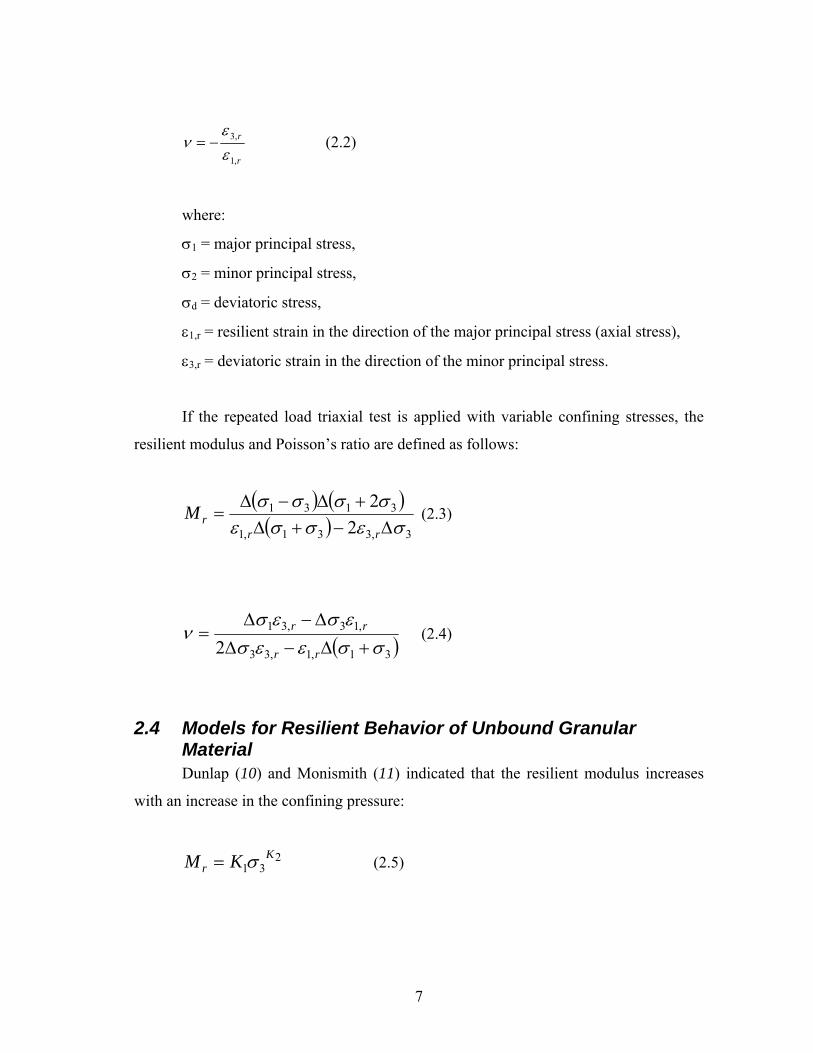
2.4 Models for Resilient Behavior of Unbound Granular Material Dunlap (10) and Monismith (11) indicated that the resilient modulus increases
with an increase in the confining pressure:
231
Kr KM σ= (2.5)

8
where
K1 and K2 = regression constants,
σ3 = the minor principal stress.
Seed (12), Brown and Pell (13) and Hicks (14) found that it is necessary to
include the applied axial stress in the analysis so they suggested the following model
which is commonly known as K-θ model:
21
Kr KM θ= (2.6)
where
θ = sum of principal stresses.
The K-θ model is simple and has been widely used for analysis of stress
dependence of material stiffness. However, the model neglects the effect of the shear
stress and is therefore applicable only in the range of low strain values. Uzan (3) noticed
that the resilient modulus is a function not only of bulk stress but also of the shear stress.
Uzan (3) included deviatoric stress and expressed the resilient modulus as follows:
321
1
K
a
octK
aar PP
IPKM ⎟⎟
⎠
⎞⎜⎜⎝
⎛⎟⎟⎠
⎞⎜⎜⎝
⎛=
τ (2.7)
where
τoct = octahedral shear stress,
I1 = sum of principal stress (θ),
Pa = atmospheric pressure,
K1, K2, and K3 = regression coefficients that depend on material properties.

9
Elliot and Lourdesnathan (15) noticed that the Uzan model fits the data very well
for pre failure stresses but when the stresses exceeded the static failure the predictions
were poor. So they suggested adding the failure term for the previous model:
1
2
1 10 A
K
r kM θ= (2.8)
where
A = failure term.
Several models have been proposed for the resilient behavior based on
decomposing both stresses and strains into volumetric and shear components. Boyce
(16) assumed the material to be nonlinear isotropic and proposed the following equations
for the volumetric (εv) and shear (εs) strains:
⎥⎥⎦
⎤
⎢⎢⎣
⎡−= 2
2
11pK
p dAv
σβε (2.9)
⎟⎟⎠
⎞⎜⎜⎝
⎛=
pGp dA
sσ
ε31 (2.10)
where
p = hydrostatic stress,
G = shear modulus,
K = bulk modulus.

10
Brown and Pappin (17) proposed the following relationships for the volumetric
and shear strains:
⎥⎥⎦
⎤
⎢⎢⎣
⎡
⎟⎟
⎠
⎞
⎜⎜
⎝
⎛⎟⎟⎠
⎞⎜⎜⎝
⎛−⎟
⎠⎞
⎜⎝⎛=
2
1p
CAp d
B
vσ
δε (2.11)
F
m
drds p
PEP
D⎥⎥⎦
⎤
⎢⎢⎣
⎡ +⎥⎦
⎤⎢⎣
⎡+
=22 σσ
δε (2.12)
where:
vε = recoverable volumetric strain,
sε = shear strain,
P = mean normal stress,
dσ = deviatoric Stress.
Several studies [Tutumluer, (4); Tutumluer and Thompson, (18), Hornych et al.
(19)] suggested that the use of anisotropic models better represent the behavior of
granular materials.
The Boyce model was modified by Hornych (19) in order to account for the
effect of anisotropy. The mathematical expressions of the anisotropic model are as
follows:
( )⎥⎥⎦
⎤
⎢⎢⎣
⎡⎟⎟⎠
⎞⎜⎜⎝
⎛−+⎟⎟
⎠
⎞⎜⎜⎝
⎛+
−+
+=
− *
*
1
2
*
*
111
0
*
312
181
32
pq
Gpq
GA
KPP
A
A
vγγγε (2.13)

11
( )⎥⎥⎦
⎤
⎢⎢⎣
⎡⎟⎟⎠
⎞⎜⎜⎝
⎛++⎟⎟
⎠
⎞⎜⎜⎝
⎛−
−+
−=
− *
*
1
2
*
*
111
0
*
6121
181
31
32
pq
Gpq
GA
KPP
A
A
sγγγε (2.14)
Triaxial testing was conducted using a machine capable of applying dynamic
loads in the axial and radial directions (18). The results obtained from this test showed
definite directional dependency (anisotropy) of aggregate moduli. The resilient moduli in
the vertical and radial directions varied with the applied stress states. It was noticed that
the vertical modulus in the vertical direction is more than that for horizontal direction for
unbound materials. However, this relationship was reversed in the case of sandy gravel
with high fines content and if the specimen was compacted at the wet side of optimum.
Five cross-anisotropic material properties are needed to define an anisotropic
material under conditions of axial symmetry: the horizontal resilient modulus ( HRM ),
the vertical dynamic modulus )( vRM , the shear modulus )( RG , the horizontal
Poisson’s ratio )( Hv , and the vertical Poisson’s ratio )( Vv . These properties are
defined as follows:
vertical
dVRM
εσ
= (2.15)
horizontal
HRM
εσ3= (2.16)
( )horizontalvertical
dRG
εεσ−
=2
(2.17)

12
1_
2_
horizontal
horizontalH ε
εν −= (2.18)
vertical
horizontalV ε
εν −= (2.19)
εhorizontal_1 is the applied horizontal strain, and εhorizontal_2 is the measured
horizontal strain 90o from the applied horizontal strain.
32
11
K
a
dK
aa
VR PP
IPKM ⎟⎟
⎠
⎞⎜⎜⎝
⎛⎟⎟⎠
⎞⎜⎜⎝
⎛=
σ (2.20)
651
4
K
a
dK
aa
HR PP
IPKM ⎟⎟⎠
⎞⎜⎜⎝
⎛⎟⎟⎠
⎞⎜⎜⎝
⎛=
σ (2.21)
981
7
K
a
dK
aaR PP
IPKG ⎟⎟⎠
⎞⎜⎜⎝
⎛⎟⎟⎠
⎞⎜⎜⎝
⎛=
σ (2.22)
As it was mentioned before the advantage of modeling granular materials using
cross anisotropic nonlinear elasticity is to predict the dilative granular material behavior
(20). Figure 2.1 shows the variation of principal strain ratios with increasing major to
minor principal stress ratios. Any value less than two for the stress ratio corresponds to
the case of elastic dilation. The nonlinear anisotropic model matches very well the
experimental values. On the other hand, under the assumption of linear isotropy,
modeling of the dilative behavior could be achieved when the Poisson’s ratio is more
than 0.5.

13
2.5 Models for Permanent Deformation of Unbound Granular Material The deformational response of the granular materials can be defined under
repeated, traffic-type loading by a resilient response which is important for load carrying
ability and permanent strain response which characterizes the long-term performance of
the pavement and rutting phenomenon. Few studies have been conducted to model the
permanent deformation of granular materials.
Several factors affect the plastic behavior in the unbound granular materials;
these factors include, stress, principal stress reorientation, number of load applications,
moisture content, stress history, density and fine contents, grading and aggregate type
(21).
There are several models used to characterize the permanent deformation
properties and to predict the permanent strain in unbound granular materials.
Barksdale (22) found that by using the repeated load triaxial tests with 105 load
applications, the accumulation of permanent axial stain was proportional to the
logarithm of the number of load cycles and expressed as follows:
( )NbaP log,1 +=ε (2.23)
where
N = number of load repetitions,
εl,P = permanent strain,
a and b = regression parameters.
Bonaquist and Witczak (23) developed a model based on the flow theory of
plasticity. This model defines the magnitude of the permanent strain occurring during the
first cycle of loading. Under repeated loading the permanent strain at any load cycle can
be expressed as a power function of permanent strain during the first load cycle. The
total permanent strain will be the sum of the permanent strain in each cycle.

14
ihNP Nεεε ∑∑ ==
1,1 (2.24)
where:
εi = permanent strain in the first load cycle,
εN = permanent strain for load cycle N.
The Hyperbolic Model developed by Duncan and Chang (24) is used to predict
the plastic strain by using static triaxial tests. The results from this test are then used to
relate the permanent axial strain to the ratio of repeated deviator stress and constant
confining pressure. The model is expressed as:
( ) ( )( ) ⎥
⎦
⎤⎢⎣
⎡−
+−
=
φφσφ
σσε
sin1sincos2/
1
/3
3,1 CR
afq
bd
p (2.25)
where:
εp = the axial plastic strain,
C = cohesion,
φ = angle of internal friction,
R = the ratio of measured strength to ultimate hyperbolic strength.
Models developed by Tseng and Lytton (25) are used to estimate the permanent
deformation of asphalt, base and subgrade materials. The basic relationship is:
( ) heN vN
ra ε
εε
δβρ
⎟⎠⎞
⎜⎝⎛−
⎟⎟⎠
⎞⎜⎜⎝
⎛= 0 (2.26)

15
where:
aδ = permanent deformation for layer/sublayer,
vε = average vertical resilient strain in the layer/sublayer as obtained from the
primary response model,
h = thickness of layer/sublayer,
rε = resilient strain imposed in laboratory test to obtain material
properties βρε and,0 .
The ratiorε
ε 0 , β and ρ are estimated according to the type of materials
investigated. For granular base, the ratio can be estimated using the following form:
rCr
EW 000003.003077.06626.80978.log 0 +−−=⎟⎟⎠
⎞⎜⎜⎝
⎛θσ
εε
(2.27)
rC EW 0000015.001806.03105.919.log −++−= θσβ (2.28)
rCC EWW 0000105.002074.003784.45062.178667.1log 22 −−++−= θθ σσρ
(2.29)
For subgrade, the model parameters can be estimated using the following
relationships:
rdCr
EW log91219.11921.09121.69867.1log 0 +−+−=⎟⎟⎠
⎞⎜⎜⎝
⎛σ
εε
(2.30)
θσσσβ 22 00000338.017165.0000278.973.log Cddc WW −+−−=
(2.31)

16
θσσσρ 22 00000545.4026.0000681.009.11log Cddc WW +−+=
(2.32)
The above equations are modified from the ones published by Tseng and Lytton.
It was found, based on discussion with Dr. Lytton that signs errors where in the paper by
Tseng and Lytton.
Some researchers developed computational procedures for pavement analysis
based on the Shakedown Theory (26). According to the Shakedown Theory, if the
applied load exceeds a limiting value called a shakedown load the pavement will show a
progressive accumulation of plastic strains under repeated loading. On the other hand if
the applied loads are lower that the shakedown limit, the pavement will be able to adapt
the loads. So the response for the pavement will be totally resilient under the load
applications.
The Vesys computer program is used to predict the rut depth based on the
assumption that the permanent strain is proportional to the resilient strain by
( ) αεµε −= NNp (2.33)

17
where
( )Npε = permanent or plastic strain due to a single load application at Nth
application,
ε = elastic or resilient strain at the 200th repetition,
N = load application number,
µ = permanent deformation representing the constant of proportionality between
permanent and elastic strain,
α = the permanent deformation indicating the rate of decrease in permanent
strain with number of load applications.
FIGURE 2.1 Variation of principal strain ratios with principal stress ratios for the HD1 material.

18

19
CHAPTER 3 — SENSITIVITY ANALYSIS OF PAVEMENT RESPONSE USING DIFFERENT STRUCTURAL MODELS
AND COMPARISON WITH AASHO ROAD MEASUREMENTS
3.1 Introduction This chapter includes a comparison between the pavement deflections calculated
using isotropic and anisotropic nonlinear models for the unbound layers and the field
deflection measurements in the AASHO Road Test. The comparison is conducted based
on deflection measurements rather than the measured performance in order to the
comparison not to be affected by the assumptions made in the empirical transfer
functions typically used in performance predictions.
The asphalt layer is assumed to be linear isotropic while the base and subbase
layer are modeled using nonlinear isotropic and nonlinear anisotropic properties. The
subgrade is modeled using nonlinear isotropic properties. The analysis includes a total of
246 sections with different layer thicknesses. The applied loads in the AASHO test
varied from 6000 to 30000psi (single axle load). The material properties for all layers are
obtained from the experimental measurements by Finn et al. (8).
3.2 AASHO Road Test 3.2.1 Background of the AASHO Road Test The AASHO Road Test near Ottawa, Illinois, was performed over a two-year
period to develop a design methodology for asphalt and concrete pavements (27, 28).
The test facilities consisted of four major loops numbered from 3 through 6 and two
smaller loops. All vehicles had the same axle arrangements-axle load combinations to
any one traffic lane of Loops 2 through 6. The same materials were used in all the major
loops as listed in Table 3.1.

20
TABLE 3.1 DESCRIPTION OF MATERIALS USED IN THE MAJOR LOOPS OF THE AASHO ROAD TEST
Layer Material
Hot Mix Asphalt
• Crushed limestone coarse aggregate
• Natural siliceous coarse sand
• Mineral filler which was limestone dust
• Penetration Grade asphalt cement (85-100
pen)
Base Crushed Dolomitic Limestone
Subbase Sand-Gravel mixture
Subgrade A-6
The loops were subjected to traffic for more than two years. The traffic was
operated at 35 mph on the test sections over 18 hrs with periods of 40 minutes each day
for 6 days a week. The traffic was extended to 7 days a week during the first 6 months of
1960.
The major loops included a total of 468 sections. Each test section was 12-ft
wide, and most of them were 100 or 160-ft long. Each loop included pavement sections
with three different thicknesses of asphalt concrete surfacing, three different thicknesses
of crushed limestone base, and three different thicknesses of sand-gravel subbase.
The applied axle load over the test sections ranged from a 2,000 lb single axle
load in one lane and a 6000 lb single axle load in the other lane in Loop 2. Loop 6 was
subjected to a 30,000 lb single axle load in one lane and a 48,000 lb tandem axle load in
the other. Table 3.2 summarizes the variables in the major sections.

21
TABLE 3.2 MATERIALS AND LOADS USED IN THE AASHO TEST Loop
Item 1 2 3 4 5 6
No traffic 2,000 S 12,000 S 18,000 S 22,400 S 30,000 S Test axle loading (Ib)
6,000 S 24,000 T 32,000 T 40,000 T 48,000 T
Factorial test sections 48 44 60 60 60 60
Special study sections 16 24 24 24 24 24
Asphalt Concrete Surfacing Thicknesses (in)
1,3,5 0,1,2,3 2,3,4 3,4,5 3,4,5 4,5,6
Base thicknesses (in) 0,6 0,3,6 0,3,6 0,3,6 3,6,9 3,6,9
Subbase thicknesses (in) 0,8,16 0,4 0,4,8 4,8,12 4,8,12 8,12,16
3.2.2 Field Deflection Measurements and Material Properties
3.2.2.1 Field Deflection Measurements Deflection measurements of the pavement surface are important for the
evaluation of the performance of a flexible pavement structure and rigid pavement load
transfer. The surface deflection is a function of many factors used in the design of the
pavement such as traffic (type and volume), pavement structural section, temperature,
and moisture. Thus, many characteristics of a flexible pavement can be determined by
measuring its deflection in response to load. The advantage of using deflection to
compare with analytical solutions is that no empirical transfer functions are used in this
comparison as is the case in performance predictions.
Surface deflection is measured as a pavement surface's vertical deflected
distance as a result of an applied (either static or dynamic) load. In the AASHO test, the
deflection of a pavement surface was measured using the Benkelman beam under
vehicle wheels moving at creep speeds (approximately 2 mph). The Benkelman Beam

22
consists of a simple lever arm supported by 3 legs (Figure 3.1). The Benkelman Beam
was used with a loaded truck - typically 80 kN (18,000 lb) on a single axle with dual
tires inflated to 480 to 550 kPa (70 to 80 psi). The tip of measuring arm was placed
between the dual tires of a truck. As the truck moved at the creep speed, the device
recorded the rebound deflection of the pavement surface. The measured deflection for
each test consisted of the mean of four measurements; two in the inner and two in the
outer wheel path.
FIGURE 3.1 A Schematic of the Benkelman Beam.
Two series of deflection measurements were conducted in the AASHO Road
Test. The first series included the deflections in the fall of 1958, while the second series
included the deflections in the spring of 1959. The fall period was selected because the
highway was completed and opened to traffic at that time. The spring period was
selected because there was a big chance of distress occurrence that time due to the higher
moisture contents of the base and subbase that existed in the spring. Table 3.3 shows the
loads used in the deflection measurements.

23
TABLE 3.3 LOADS USED IN DEFLECTION STUDIES
Loop Lane Single Axle Load (Kips)
1 - 2 2 6 1 12 3 2 12 1 12,18 4 2 12 1 12, 22.4 5 2 12 1 12,30 6 2 12
3.2.2.2 Seasonal Material Characterization Since the performance of the pavements varies from season to season, it was
necessary to analyze the AASHO Road Test pavement in different seasons (29). Finn et
al. (8) characterized the properties of the materials used in the AASHO Road Test
including the asphalt surfacing, base, subbase and subgrade. The evaluation of the
seasonal material properties was conducted using laboratory triaxial testing. The resilient
moduli for the base and subbase materials were expressed as function of the first stress
invariant, while the subgrade materials were modeled as a function of the deviatoric
stress.
The modulus of the asphalt concrete was measured at the average temperature of
the AASHO Road Test location during the traffic testing. The resilient moduli of the
base materials were measured at density values representing the construction values, and
using three different water contents to take into account the seasonal variation (water
content = 4.2%, 5.6%, and 1.5%).
The subbase material modulus was measured at the optimum water content
(3.8%) and at the saturation water content (6.4%). The subgrade modulus was
determined using a trial and error procedure such that the calculated surface deflections
using a linear elastic program had the best match with field measurements. The material

24
moduli are shown in Table 3.4. The Poisson’s ratio was assumed constant for each
material, and the values in Table 3.5 were assigned for the different layers.
TABLE 3.4 ELASTIC MODULI OF AASHO ROAD TEST MATERIALS
Material Moduli
Asphalt
concrete
Base Subbase Subgrade Seasons
psi (kPa) psi (kPa) psi (kPa) psi (kPa)
Spring 0.71×10⁶
(4.9×10⁶)
3200 6.0θ
(6900 6.0θ )
4600 6.0θ
(10000 6.0θ )
8000 06.1−dσ
(427000 06.1−dσ )
Fall 0.45×10⁶
(3.1×10⁶)
4000 6.0θ
(8700 6.0θ )
5400 6.0θ
(11700 6.0θ )
27000 06.1−dσ
(1440000 06.1−dσ )
Summer 0.23×10⁶
(1.6×10⁶)
3600 6.0θ
(7800 6.0θ )
5000 6.0θ
(10800 6.0θ )
18000 06.1−dσ
(960000 06.1−dσ )
Winter 1.7×10⁶
(11.7×10⁶)
50000
(34500)
50000
(345000)
50000
(345000)
TABLE 3.5 POISSON’S RATIO OF AASHO ROAD TEST MATERIAL
Material Poisson’s ratio
Asphalt 0.3
Granular base 0.4
Granular subbase 0.4
Fine grained subgrade 0.45

25
3.3 Pavement Analysis A finite element program was used to calculate the deflections at the surface of
the pavement by using the materials properties given in Tables 3.4 and 3.5. Two models
were used in the finite element program to describe the base and subbase layers:
nonlinear isotropic and nonlinear anisotropic. The results were compared with the
experimental deflection measurements.
The finite element program allows the computation of the resilient response of
flexible pavement, such as stress, strain and deformation at any location in the pavement.
The program accounts for nonlinear and anisotropic elastic properties of all pavement
layers. The program uses a typical axisymmetric finite element mesh as shown in Figure
3.2. The mesh used in this analysis has a 50-in. width with 9 columns while the length is
100 in with 16 rows. The total number of elements is 144. Each element has 8 nodes.
The applied pressure is 75 psi which is equivalent to the pressure used in the Benkelman
device in the AASHO Road Test to measure the surface deflection. The loading radius
depends on the applied load which was different for the different loops.
It is known that the modulus of the unbound granular materials is stress sensitive
and changes through the layer so that the modulus of the untreated materials at any point
in the layer is a function of stress. The properties are the same in all directions
(isotropic). The resilient modulus is calculated as:
32
11
K
a
oct
K
aar PP
IPKM ⎟⎟
⎠
⎞⎜⎜⎝
⎛⎟⎟⎠
⎞⎜⎜⎝
⎛=
τ (3.1)
where
I1 = first stress invariant (sum of principal stresses),
octτ = octahedral shear stress,
Pa = atmospheric pressure.

26
K1, K2 and K3 used in the finite element model are calculated based on the
measured material properties given in Table 3.4 for the spring and fall seasons.
In the anisotropic model, equations similar to Eq. 3.1 are used to express the
vertical modulus, horizontal modulus, and shear modulus. The moduli are modeled from
the triaxial stress states using the following equations:
32
11
K
a
dK
aa
VR PP
IPKM ⎟⎟
⎠
⎞⎜⎜⎝
⎛⎟⎟⎠
⎞⎜⎜⎝
⎛=
σ (3.2)
65
14
K
a
d
K
aa
HR PP
IPKM ⎟⎟⎠
⎞⎜⎜⎝
⎛⎟⎟⎠
⎞⎜⎜⎝
⎛=
σ (3.3)
981
7
K
a
dK
aaR PP
IPKG ⎟⎟
⎠
⎞⎜⎜⎝
⎛⎟⎟⎠
⎞⎜⎜⎝
⎛=
σ (3.4)
The finite element program requires the K1, K2, K3 , n, m and µ parameters:
VR
HR
MMn = (3.5)
VR
xy
MG
m = (3.6)
xy
xx
νν
µ = (3.7)
vxx is the horizontal Poisson’s ratio, and vxy is the vertical Poisson’s ratio.

27
In this study, the base and subbase layer are assumed to be either nonlinear
isotropic or nonlinear anisotropic. In the isotropic approach, the modular ratios (n and
µ ) are set to 1. In the anisotropic analysis, the n value is taken to be 0.5, 0.4 and 0.3,
while µ is set to 1.5. These values are selected to represent experimental measurements
for a wide range of aggregates at the Texas Transportation Institute (5, 30). By assuming
the Poisson’s ratio in the base and subbase layer to be equal 0.4, the m value can be
determined by using the following equation.
( )xy
mν+
=12
1 (3.8)
The asphalt layer is modeled as linear isotropic, and the materials properties K2
and K3 are set to zero. The subgrade is modeled by nonlinear properties. Table 3.6 shows
a summary of the input data used in the FEM.

28
FIGURE 3.2 Finite element mesh for pavement analysis.
3.4 Comparison between the FEM Calculations and Measurements A comparative analysis was conducted between the finite element predictions
and the measured deflections in the AASHO road sections. The finite element program
was used to calculate the deflections at the surface of 246 different pavement sections.
The material properties for 134 sections represented the fall season, while the remaining
112 sections represented the spring season. These predicted deflections were then
compared with the deflections measured in the AASHO Road Test. The sections used
100in
HMA
Subbase
Subgrade
Base
Rq=75psi
100in

29
for this study were from Loop 2 through Loop 6 with single axle loads that ranged from
6 - 30 kip.
Figures 3.3 to 3.6 show the relationships between the field measurements in the
fall season and the finite element results using either isotropic or anisotropic material
properties. The comparisons with the measurements from the spring season are shown in
Figures 3.7 to 3.10, and the results combined for both seasons are shown in Figures 3.11
to 3.14. Deflections calculated using isotropic material properties tend to be smaller than
the experimental measurements. As the anisotropy increases (n value decreases) the
calculated deflections become closer to the measurements and the accuracy of the
prediction increases. In general, the finite element predictions are closer to
measurements in the fall season than in the spring season.
FIGURE 3.3 Measured versus calculated deflections for the fall season using isotropic properties.
n = 1.0 µ = 1.0
0
10
20
30
40
50
60
70
80
0.00
10.00
20.00
30.00
40.00
50.00
60.00
70.00
80.00
Calculated Deflection, 0.001 inch
Isotropic Equality Line
Measured Deflection, 0.001 in

30
TABLE 3.6 A SUMMARY OF THE INPUT DATA USED IN THE FEM PROGRAM (LIS: LINEAR ISOTROPIC; NIS: NONLINEAR ISOTROPIC; NAN: NONLINEAR ANISOTROPIC; NIS: NONLINEAR ISOTROPIC)
FEM Parameters Season Layer
AASHO Road
Modulus Model K1 K2 K3 n m µ vxy
Spring 0.71×10⁶ 48965.5 0 0 1 0.38 1 0.3
Fall
HMA
0.45×10⁶
LIS
31034.5 0 0 1 0.38 1 0.3
NIS 1098 0.6 0 1 0.36 1 0.4
Spring 3200θ0.6
NAN 1098 0.6 0 0.5 0.4 0.3
0.36 1.5 0.4
NIS 1372.5 0.6 0 1 0.36 1 0.4
Fall
Base
4000θ0.6
NAN 1372.5 0.6 0 0.5 0.4 0.3
0.36 1.5 0.4
NIS 1578.4 0.6 0 1 0.36 1 0.4
Spring 4600θ0.6
NAN 1578.4 0.6 0 0.5 0.4 0.3
0.36 1.5 0.4
NIS 1852.9 0.6 0 1 0.36 1 0.4
Fall
Subbase
5400θ0.6
NAN 1852.9 0.6 0 0.5 0.4 0.3
0.36 1.5 0.4
Spring 3000σd
-1.06 32.41 0 1.06 1 0.34 1
0.45
Fall Subgrade 2700σd
-1.06 NIS 109.4 0 1.06 1 0.34 1
0.45

31
n = 0.5 µ = 1.5
0
10
20
30
40
50
60
70
80
0.00 10.00 20.00 30.00 40.00 50.00 60.00 70.00 80.00
Calculated Deflection, 0.001 inch
Mea
sure
d D
efle
ctio
n, 0
.001
in
AnisotropicEquality Line
FIGURE 3.4 Measured versus calculated deflections for the fall season
using anisotropic properties with n = 0.5.
n = 0.4 µ = 1.5
0
10
20
30
40
50
60
70
80
0.00 10.00 20.00 30.00 40.00 50.00 60.00 70.00 80.00
Calculated Deflection, 0.001 inch
Mea
sure
d D
efle
ctio
n, 0
.001
in
AnisotropicEquality Line
FIGURE 3.5 Measured versus calculated deflections for the fall season
using anisotropic properties with n = 0.4.

32
n = 0.3 µ = 1.5
y = 0.9074x + 3.6903R2 = 0.6221
0
10
20
30
40
50
60
70
80
0.00 10.00 20.00 30.00 40.00 50.00 60.00 70.00 80.00
Calculated Deflection, 0.001 inch
Mea
sure
d D
efle
ctio
n, 0
.001
in
AnisotropicEquality LineLinear (Anisotropic)
FIGURE 3.6 Measured versus calculated deflections for the fall season
using anisotropic properties with n = 0.3.
n = 1.0 µ = 1.0
0
10
20
30
40
50
60
70
80
0.0 10.0 20.0 30.0 40.0 50.0 60.0 70.0 80.0
Calculated Deflection, 0.001 inch
Mea
sure
d D
efle
ctio
n, 0
.001
in
IsotropicEquality Line
FIGURE 3.7 Measured versus calculated deflections for the spring season
using isotropic properties.

33
n = 0.5 µ = 1.5
0
10
20
30
40
50
60
70
80
0.0 10.0 20.0 30.0 40.0 50.0 60.0 70.0 80.0
Calculated Deflection, 0.001 inch
Mea
sure
d D
efle
ctio
n, 0
.001
in
AnisotropicEquality Line
FIGURE 3.8 Measured versus calculated deflections for the spring season using
anisotropic properties with n = 0.5.
n = 0.4 µ = 1.5
0
10
20
30
40
50
60
70
80
0.0 10.0 20.0 30.0 40.0 50.0 60.0 70.0 80.0
Calculated Deflection, 0.001 inch
Mea
sure
d D
efle
ctio
n, 0
.001
in
AnisotropicEquality Line
FIGURE 3.9 Measured versus calculated deflections for the spring season using
anisotropic properties with n = 0.4.

34
n = 0.3 µ = 1.5
y = 1.1118x + 3.8117R2 = 0.6179
0
10
20
30
40
50
60
70
80
0.0 10.0 20.0 30.0 40.0 50.0 60.0 70.0 80.0
Calculated Deflection, 0.001 inch
Mea
sure
d D
efle
ctio
n, 0
.001
in
Anisotropic
Equality Line
Linear(Anisotropic)
FIGURE 3.10 Measured versus calculated deflections for the spring season using
anisotropic properties with n = 0.3.
n = 1.0, µ = 1.0
0
10
20
30
40
50
60
70
80
0.00 10.00 20.00 30.00 40.00 50.00 60.00 70.00 80.00
Calculated Deflection, 0.001 inch
Mea
sure
d D
efle
ctio
n, 0
.001
in
IsotropicEquality Line
FIGURE 3.11 Measured versus calculated deflections for the spring and fall seasons
using isotropic properties.

35
n = 0.5, µ = 1.5
0
10
20
30
40
50
60
70
80
0.00 10.00 20.00 30.00 40.00 50.00 60.00 70.00 80.00
Calculated Deflection, 0.001 inch
Mea
sure
d D
efle
ctio
n, 0
.001
in
Anisotropic Equality Line
FIGURE 3.12 Measured versus calculated deflections for the spring and fall season
using anisotropic properties with n = 0.5.
n = 0.4, µ = 1.5
0
10
20
30
40
50
60
70
80
0.00 10.00 20.00 30.00 40.00 50.00 60.00 70.00 80.00
Calculated Deflection, 0.001 inch
Mea
sure
d D
efle
ctio
n, 0
.001
in
AnisotropicEquality Line
FIGURE 3.13 Measured versus calculated deflections for the spring and fall season
using anisotropic properties with n = 0.4.

36
FIGURE 3.14 Measured versus calculated deflections for the spring and fall season using anisotropic properties with n = 0.3.
The accuracy of the calculations in predicting the measurements was studied by
calculating the percentage of error which is the absolute difference between the
calculated and measured values divided by the measured value. The cumulative
distribution function of errors is shown in Figures 3.15 to 3.17. The y axis represents the
percentage of data points with an error equal to or less than the corresponding value on
the x axis. The results clearly show that the anisotropic model reduces the percentage of
errors. This point can also be shown in Figures 3.18 to 3.20, which show the number of
data points that belong to different error levels. Again, it can be seen that the number of
data points shift from high error ranges to small error ranges as anisotropy increases.
n = 0.3, µ = 1.0
y = 1.0978x + 0.7322 R2 = 0.6333
0
10
20
30
40
50
60
70
80
0.00 10.00 20.00 30.00 40.00 50.00 60.00 70.00 80.00 Calculated Deflection, 0.001 inch
Measured Deflection, 0.001 in
Anisotropic
Equality Line
Linear(Anisotropic)

37
0
10
20
30
40
50
60
70
80
90
100
0 10 20 30 40 50 60
Percent Error, %
Cum
ulat
ive
Dist
ribut
ion
Func
tion
Isotropic n=0.3
FIGURE 3.15 Percentage error for isotropic and anisotropic (n=0.3) predictions
for the fall season.
0
10
20
30
40
50
60
70
80
90
100
0 10 20 30 40 50 60Percent Error, %
Cum
ulat
ive
Dis
tribu
tion
Func
tion
Isotropic n=0.3
FIGURE 3.16 Percentage error for isotropic and anisotropic (n=0.3) predictions
for the spring season.

38
0
10
20
30
40
50
60
70
80
90
100
0 10 20 30 40 50 60 70
Percent Error, %
Cum
ulat
ive
Dist
ribut
ion
Func
tion
Isotropic n=0.3
FIGURE 3.17 Percentage error for isotropic and anisotropic (n=0.3) predictions for the
fall and spring seasons.
0
5
10
15
20
25
0 5 10 15 20 25 30 35 40 45 50 55 60 65
Percentage of Error
Num
ber o
f Dat
a Po
ints
n = 1.0 n = 0.3
FIGURE 3.18 Number of points within a certain range of percent of error for the spring
season.

39
0
10
20
30
40
50
60
0 5 10 15 20 25 30 35 45 50 55 60 65 70
Percentage of Error
Num
ber o
f Dat
a Po
ints
n = 1.0 n = 0.3
FIGURE 3.19 Number of points within a certain range of percent of error for the spring and fall seasons.
0
5
10
15
20
25
30
0 5 10 15 20 25 30 35 45 50 55 60 65 70 75 80
Percentage of Error
Num
ber o
f Poi
nts
n = 1.0 n = 0.3
FIGURE 3.20 Number of points within a certain range of percent of error
for the fall season.

40
3.5 Summary of Findings In this chapter, a finite element program was used to calculate deflections of
sections resembling the AASHO Road Test. These calculations were compared to the
field experimental measurements. The following points summarize the findings:
Anisotropy was modeled by the ratio of the horizontal modulus to vertical
modulus. The percentage of error between predictions and measurements decreased as
the anisotropy increased.
The FEM predictions correlated the best with the experimental measurements
when the horizontal modulus was about 30% of the vertical modulus.
The predictions matched the AASHO measurements in the fall season better than
the measurements in the spring season. As reported in the AASHO experiment,
distresses were detected in the spring season that might have caused the response to
deviate from the elastic solutions used in the FEM.
41
CHAPTER 4 — ANALYSIS OF FLEXIBLE PAVEMENT RUTTING AND FATIGUE CRACKING USING ISOTROPIC
AND ANISOTROPIC RESPONSE MODELS
4.1 Introduction This chapter presents predictions of permanent deformation and fatigue cracking
based on the mechanistic-empirical models used in the AASHTO 2002. These models
utilize elastic stress and strain values, which are calculated in this chapter using a finite
element program with the base course represented by linear isotropic, nonlinear
isotropic, linear cross-anisotropic or nonlinear cross-anisotropic properties. Comparisons
between the performance predictions of rutting and fatigue cracking using these different
models are reported in this chapter.
4.2 Fatigue Cracking Models in the AASHTO 2002 Guide Fatigue cracking is one of the most important distresses occurring in flexible
pavements. The repeated traffic induces tensile and shear stresses in the bound layer.
The repeated load initiates cracks at the point of critical tensile stress. The location of the
critical tensile stress depends on the stiffness of the layer.
It is typically assumed that the fatigue cracking normally occurs at the bottom of
the asphalt layer and propagates to the surface. In order to predict the allowable number
of load repetitions for fatigue cracking to occur in the flexible pavement, the tensile
strain at the bottom of the HMA layer is considered as the critical strain. This type of
cracking (bottom-up cracking) is actually due the bending action of the pavement layer.
However most recent studies show that fatigue cracking may initiate from the top and
propagate down (top-down). The top-down cracking is caused by large contact pressures
at the tire edge-pavement interface where the top layer of the pavement has been
oxidized (6). In this case, the critical point for the tensile strain will be at the surface of
the layer or at 0.5 in. from the top (6). The different versions of the AASHTO 2002

42
released until the point of the preparation of this thesis included two models for fatigue
which are discussed herein.
The model used to find the allowable number of load repetition has the following
form:
32 111
kk
tf E
CkN ⎟⎠⎞
⎜⎝⎛
⎟⎟⎠
⎞⎜⎜⎝
⎛=
ε (4.1)
( ) ( ) 32 *1
Kkt ECk −−= ε (4.2)
where:
fN = number of repetitions to fatigue cracking,
tε = tensile strain at the critical location,
E = stiffness of the material,
321 ,, kkk = laboratory calibration parameters,
C = laboratory to field adjustment factor.
The fatigue model in the AASHTO 2002 Design Guide released in December
2002 is based on the Shell Oil Fatigue Model. The most important terms in this model
are the stiffness of the asphalt layer and the tensile strain at the point of critical location.
The critical location may be at the top of the layer for the top-down cracking or at the
bottom for the bottom-up cracking.
Two types of controlled loading are used in the laboratory for fatigue cracking
the constant stress and constant stain. Constant stress loading is considered applicable
when the thickness of the layer is more than 8 inches, while constant strain is applicable
for thin layers less than two inches. Shell Oil has developed equations to predict fatigue
cracking for these two cases. These equations are summarized below:

43
Constant Strain: ( )[ ] 8.155
112.00454.00085.017.0 −−−+−= EVVPIPIAN tbff ε
(4.3)
Constant Stress: ( )[ ] 4.1550167.000673.000126.0252.0 −−−+−= EVVPIPIAN tbbff ε
(4.4)
where
PI = penetration index,
Vb = volume of bitumen.
Since the thickness for the asphalt layer could be between 2 and 8 inches which
is not included in these equations, a new equation is developed in the AASHTO 2002
Design Guide to take into account the intermediate thickness (between 2 and 8 inches)
based on equations 4.3 and 4.4. The generalized Shell Oil fatigue equation is as follows:
( ) ( )( )4.1
*5
408.5354.1
4.0 110167.000673.000126.00252.0exp1
1139091−
−
−
⎟⎠⎞
⎜⎝⎛
⎟⎟⎠
⎞⎜⎜⎝
⎛−+−⎟⎟
⎠
⎞⎜⎜⎝
⎛
+−
+=E
VVPIPIECNt
bbhfac ε
(4.5)
( )408.5354.1
4.0''
exp11139091 −
−
+−
+=ach
EF (4.6)
( )[ ]51 0167.000673.000126.00252.0 −+−= bb VVPIPIK α (4.7)

44
where
C = laboratory to field adjustment factor; with a default value of 1.0,
hac = thickness of the asphalt layer,
tε = tensile strain,
E = stiffness of the material,
PI = penetration index,
Vb = volume of bitumen.
The fatigue model used in the AASHTO 2002 Design Guide released in
November 2003 was based on the Asphalt Institute Method. However, the equations
were modified using calibration factors based on data collected from 82 LTPP sections
located in 24 states, and to accommodate pavements with different thicknesses. The
model has the form in Equations 4.8 – 4.12:
( ) ( ) 33*2211
kfkftff EkN
ββεβ−−= (4.8)
281.19492.3'1
11**00432.0 ⎟⎠⎞
⎜⎝⎛
⎟⎟⎠
⎞⎜⎜⎝
⎛=
ECkN
tf ε
(4.9)
MC 10= (4.10)
⎟⎟⎠
⎞⎜⎜⎝
⎛−
+= 69.084.4
ba
b
VVV
M (4.11)

45
( )ache
k
*49.302.11
'1
1003602.0000398.0
1
−++
= (4.12)
where:
321 ,, fff βββ = calibration parameters,
Va = percent air voids,
Vb = effective binder content,
hac = total thickness of the asphalt layer, '1k = correction for different asphalt layer thickness effects.
4.3 Analysis of Fatigue Cracking Using Isotropic and Anisotropic Models The base layer and the asphalt mix are modeled using linear isotropic, nonlinear
isotropic, linear cross-anisotropic or nonlinear cross anisotropic properties. The
parameters K1, K2, K3, n, m and µ in Eqs. 3.2 to 3.8 for the different pavement layers is
shown in Table 4.1. vxx is the horizontal Poisson’s ratio, and vxy is the vertical Poisson’s
ratio. The linear isotropic properties are determined by taking K2 and K3 to be zero,
while n and m are assigned to unity. Six sections are used in the analysis. Sketches of
these sections are shown in Figure 4.1.

46
TABLE 4.1 PAVEMENT MATERIAL PROPERTIES
HMA Layer (2, 4, 6 in.)
LIS NIS LAN NAN
K1 = 28000 K2=0
K3= 0 n=1.0
m=0.38 µ=1.0
υxy=0.35
K1 = 28000 K2=0.1
K3= 0 n=1.0
m=0.38 µ=1.0
υxy=0.35
K1 = 28000 K2=0
K3= 0 n=0.5
m=0.38 µ=1.5
υxy=0.35
K1 = 28000 K2=0.1 K3= 0 n=0.5
m=0.38 µ=1.5
υxy=0.35
Base Layer (12, 18 in.)
LIS NIS LAN NAN
K1 = 2069 K2=0
K3= 0 n=1.0 m=0.38 µ=1.0
υxy=0.35
K1 = 2069 K2=0.455
K3= 0.295 n=1.0
m=0.38 µ=1.0
υxy=0.35
K1 = 2069 K2=0
K3= 0 n=0.5
m=0.38 µ=1.5
υxy=0.35
K1 = 2069 K2=0.455 K3= 0.295 n=0.5
m=0.38 µ=1.5
υxy=0.35
Subgrade
LIS NIS
K1 = 345 K2=0 K3=0
n=1.0 m=0.38 µ=1.0 n=1.0
υxy=0.4
K1 = 345 K2=0 K3=-0.3
m=0.38 µ=1.0
υxy=0.4

47
Section (A) Section (B) Section (C)
Section (D) Section (E) Section (F)
FIGURE 4.1 The sections used in the analysis.
The fatigue analysis is conducted using the Shell Model and Asphalt Institute
Model calibrated in the AASHTO 2002 design guide. The tensile strain at the bottom of
the HMA layer was considered as the critical strain for bottom-top cracking.
400,000psi
υ=0.35 2in 4in 6in 30000PSI υ=0.35
18in
18in18in
5000psi υ=0.4
400,000psi
υ=0.35 2in 4in 6in 30,000psi υ=0.35
12in
12in12in
5000psi υ=0.4

48
The Shell equation was used with typical values for the penetration index (0.934)
and volume of bitumen (11%). Figures 4.2 and 4.3, show the fatigue life using the
isotropic and anisotropic material properties.
1.97E+051.89E+05
1.56E+05
1.69E+05
1.13E+05
1.49E+05
2.13E+05
1.90E+052.01E+05
1.92E+05
1.50E+05
1.76E+05
0.0E+00
5.0E+04
1.0E+05
1.5E+05
2.0E+05
2.5E+05
Nf
Fatigue Cracking
LIS LAN
FIGURE 4.2 Comparison between linear isotropic and linear anisotropic models of the
allowable number of load repetitions using the Shell method.
Section (A) Section (B) Section (C) Section (D) Section (F) Section (E)

49
5.80E+04
1.05E+05
3.60E+04
4.69E+04
3.18E+04
3.75E+04
4.41E+04
1.06E+05
3.72E+04
4.79E+04
3.40E+043.80E+04
0.0E+00
2.0E+04
4.0E+04
6.0E+04
8.0E+04
1.0E+05
1.2E+05
Nf
Fatigue Cracking
NIS NAN
FIGURE 4.3 Comparison between non-linear isotropic and non-linear anisotropic
models of the allowable number of load repetitions using the Shell Method.
It can be seen form Figure 4.2 that the anisotropic model starts to give higher
number of load repetitions than the isotropic models when the thickness of the HMA
layer increases in the linear analysis. In the case of nonlinear analysis, it can be seen that
the anisotropic model gives longer fatigue life than the isotropic model. These results
can explain part of the shift factor between the laboratory fatigue life and the field
fatigue life. It is clear that using anisotropic properties predicts longer fatigue life and
less shift factor.
Figure 4.4 shows a comparison between the linear isotropic and linear
anisotropic models based on the tensile strain distribution across the depth of the asphalt
and base layer. It can be seen from this figure that the tensile strain at the bottom of
HMA for the isotropic model is more than that for the anisotropic model. Appendix A
includes the strain profiles for the sections in Figure 4.1 calculated using the different
models in Table 4.1.
Section (A) Section (B) Section (C) Section (D) Section (F) Section (E)

50
Tensile Strain VS Depth ,Section C
3
6
9
12
15
18
1.4E-04 1.6E-04 1.8E-04 2.0E-04 2.2E-04 2.4E-04 2.6E-04 2.8E-04
Tensile Strain
Dep
th (i
n)
lis lan
FIGURE 4.4 The tensile strain profiles in the asphalt and base layers of Section C using linear isotropic and anisotropic properties.
Tensile Strain VS Depth ,Section A
0
2
4
6
8
10
12
14
16
3.0E-04 4.0E-04 5.0E-04 6.0E-04 7.0E-04 8.0E-04 9.0E-04
Tensile Strain
Dep
th (i
n)
nis nan
FIGURE 4.5 The tensile strain profiles in the asphalt and base layers of Section A using nonlinear isotropic and anisotropic properties.

51
The Asphalt Institute Equation (Eq. 4.9) was also used to determine the fatigue
life using a volume of bitumen of 11% and percentage air voids in the asphalt mix equal
to about 7.5%. Figures 4.6 and 4.7 show comparisons in fatigue life using isotropic and
anisotropic material properties. The results are in accordance with those from the Shell
Method. More specifically, the nonlinear anisotropic analysis predicts longer fatigue life
than the nonlinear isotropic analysis.
6.98E+066.74E+06
1.14E+06 1.21E+06
3.86E+06
4.78E+06
7.42E+06
6.78E+06
1.39E+06 1.34E+06
4.81E+06
5.45E+06
0.0E+00
1.0E+06
2.0E+06
3.0E+06
4.0E+06
5.0E+06
6.0E+06
7.0E+06
8.0E+06
Nf
Fatigue Cracking
LIS LAN
FIGURE 4.6 Comparison between linear isotropic and linear anisotropic models of the
allowable number of load repetitions using the Asphalt Institute Method.
Section (A) Section (B) Section (C) Section (D) Section (F) Section (E)

52
2.6E+06
4.3E+06
3.51E+05 4.34E+05
1.39E+061.59E+06
2.10E+06
4.18E+06
3.60E+05 4.40E+05
1.47E+061.61E+06
0.0E+00
5.0E+05
1.0E+06
1.5E+06
2.0E+06
2.5E+06
3.0E+06
3.5E+06
4.0E+06
4.5E+06
Nf
Fatigue Cracking
NIS NAN
FIGURE 4.7 Comparison between nonlinear isotropic and nonlinear anisotropic models
of the allowable number of load repetitions using the Asphalt Institute Method.
The fatigue life predicted by the Asphalt Institute Model is much longer than that
predicted by the Shell Model. This discrepancy is attributed to the fact that the Asphalt
Institute method was calibrated with field data, while the Shell Method was not. It is
interesting to note that the results show that thin pavements can have longer fatigue life
than the thick pavements. This observation is consistent with the findings by the
AASHTO 2002 team that it is not necessary that the magnitude of tensile strain increases
proportionally to a decrease in HMA thickness.
4.4 Permanent Deformation Models in the AASHTO 2002 Guide Permanent deformation is one of the most important distresses occurring in the
flexible pavement. It is associated with rutting in the wheel path and develops gradually
as the number of load repetitions increase. For many years it was assumed that the
permanent deformation is related to the vertical compressive strain at the top of subgrade
so that the rutting can be reduced by limiting the vertical compressive strain at the top of
Section (A) Section (B) Section (C) Section (D) Section (F) Section (E)
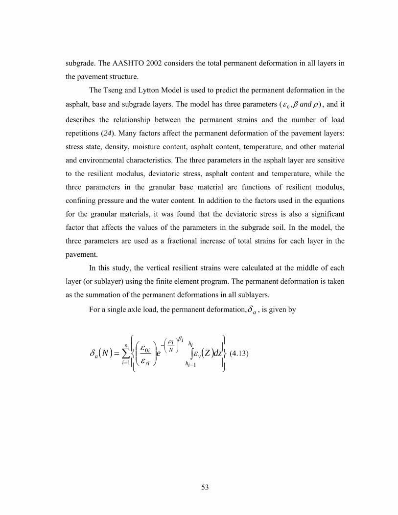
53
subgrade. The AASHTO 2002 considers the total permanent deformation in all layers in
the pavement structure.
The Tseng and Lytton Model is used to predict the permanent deformation in the
asphalt, base and subgrade layers. The model has three parameters ( ),0 ρβε and , and it
describes the relationship between the permanent strains and the number of load
repetitions (24). Many factors affect the permanent deformation of the pavement layers:
stress state, density, moisture content, asphalt content, temperature, and other material
and environmental characteristics. The three parameters in the asphalt layer are sensitive
to the resilient modulus, deviatoric stress, asphalt content and temperature, while the
three parameters in the granular base material are functions of resilient modulus,
confining pressure and the water content. In addition to the factors used in the equations
for the granular materials, it was found that the deviatoric stress is also a significant
factor that affects the values of the parameters in the subgrade soil. In the model, the
three parameters are used as a fractional increase of total strains for each layer in the
pavement.
In this study, the vertical resilient strains were calculated at the middle of each
layer (or sublayer) using the finite element program. The permanent deformation is taken
as the summation of the permanent deformations in all sublayers.
For a single axle load, the permanent deformation, aδ , is given by
( ) ( )∑ ∫= −
⎟⎟⎠
⎞⎜⎜⎝
⎛−
⎪⎭
⎪⎬⎫
⎪⎩
⎪⎨⎧
⎟⎟⎠
⎞⎜⎜⎝
⎛=
n
i
ih
ihv
i
Ni
ri
ia dzZeN
1 1
0 εεεδ
βρ
(4.13)

54
where
aδ = permanent deformation for layer/sublayer,
vε = average vertical resilient strain in the layer/sublayer as obtained from the
primary response model,
h = thickness of the layer/sublayer,
rε = resilient strain imposed in laboratory test to obtain material properties
βρε and,0 ,
=ρβε and,0 material properties.
The equations of the three parameters are (some of the signs in these equations
are modified here based on discussion with Dr. Lytton):
Asphalt Layer
rdcc ETAA log12228.1log203249.001127.0011045.001812.004349.5log 2 +−+++−= σβ (4.14)
rdcc ETAA 0000002.0log16597.000214.005282.060816.051475.2log 2 −+−−+−= σβ (4.15)
rdcc ETAA 000005.001487.003865.054159.0241965.4105675.8log 2 +−++−= σρ (4.16)
Granular Material
rCr
EW 000003.0003077.006626.080978.0log 0 ++−=⎟⎟⎠
⎞⎜⎜⎝
⎛θσ
εε
(4.17)
rC EW 0000015.0001806.003105.0919.0log −++−= θσβ (4.18)

55
rCC EWW 0000105.0002074.0003784.045062.178667.1log 22 −−++−= θθ σσρ (4.19)
Subgrade
rdCr
EW log91219.011921.009121.069867.1log 0 +−+−=⎟⎟⎠
⎞⎜⎜⎝
⎛σ
εε
(4.20)
θσσσβ 22 00000338.0017165.00000278.0973.0log Cddc WW −+−−=
(4.21)
θσσσρ 22 00000545.04026.00000681.0009.11log Cddc WW +−+=
(4.22)
where
=CW water content(%),
dσ = deviatoric stress (psi),
=θσ bulk stress (psi),
=rE resilient modulus of the layer/sublayer(psi).
The form of the Tseng and Lytton Model was modified in the AASHTO 2002 to
include a calibration factor:
( ) heN vN
ra ε
εε
βδβρ
⎟⎠⎞
⎜⎝⎛−
⎟⎟⎠
⎞⎜⎜⎝
⎛= 0
1 (4.23)

56
where:
1β = calibration factor for the unbound granular and subgrade materials; equal
to 2.2 for the base layer while it is equal to 8.0 for the subgrade soil.
The equations used to get the three parameters ρβε and,,0 in the base and
subgrade layers in the AASHTO 2002 are different than the ones proposed by Tseng and
Lytton. The stress term is eliminated from the equations in the AASHTO 2002. The
relationships for the base and subgrade are as follows:
cW017638.061119.0log −−=β (4.24)
( )( )2
**
log
77
17
101
0⎟⎟
⎠
⎞
⎜⎜
⎝
⎛+
=⎟⎟⎠
⎞⎜⎜⎝
⎛
⎟⎠⎞⎜
⎝⎛
br
br
r
EaeEaeβρ
βρ
εε (4.25)
( )⎥⎦
⎤⎢⎣
⎡=
77
11
0 ln br
br
EaEaC (4.26)
( )( )β
βρ
1
7
07
10110
⎥⎥⎦
⎤
⎢⎢⎣
⎡
−=
C (4.27)
1192.0*3586.0
64.01
2555712.51
GWT
rc
EW
−
⎥⎥⎥
⎦
⎤
⎢⎢⎢
⎣
⎡⎟⎠⎞
⎜⎝⎛= (4.28)

57
where:
Wc = water content (%),
Er = resilient modulus of the layer/sublayer (psi),
GWT = ground water table depth (ft),
a1 = 1.0942e-18,
b1 = 3.520049,
a7 = 0.03162278,
b7 = 0.5.
The relationship used in the AASHTO 2002 to predict the permanent
deformation in the asphalt layer is based on the statistical analysis of laboratory repeated
load permanent deformation tests.
The final equation conducted by Leahy, Ayers and Kaloush to predict the
permanent deformation is as follows:
5606..1479244.0.51108.31 10* TNK
r
p −=εε
(4.29)
342.17*4868.2*1039.0 21 −+−= acac HHC (4.30)
428.27*7331.1*0172.0 22 +−= acac HHC (4.31)
where
rε = the vertical resilient strain at any depth (obtained from the primary
response model),
N = allowable number of load repetitions,
T = temperature (F),
pε = plastic strain,

58
k1 = function of total asphalt layer thickness and depth to computational point, to
correct for the confining pressure at different depths.
The rut depth for each sublayer in the AC layer can be found from
ipidi hR ∆=∆ .ε (4.32)
The summation for all incremental dR∆ , the total layer rut depth can be obtained
from
∑=
∆=1i
did RR (4.33)
4.5 Analysis of Permanent Deformation Using Isotropic and Anisotropic Models It was found that the permanent strain calculated using anisotropic properties is
higher than using isotropic properties in the asphalt layer. An example of the results is
shown in Figure 4.8. This difference is attributed to the higher compressive strain in the
anisotropic model compared with the isotropic model, although the deviatoric stress is
less for the anisotropic model. Examples of the results are shown in Figures 4.9 and
4.10. The results for the other sections are given in Appendix A.

59
Rutting (HMA), Section C
0.04
0.05
0.06
0.07
0.08
0.09
0.1
0.11
0.12
0.13
0.14
0.0E+00 5.0E+06 1.0E+07 1.5E+07 2.0E+07 2.5E+07
Number of load repetitions
Per
man
ent D
efor
mat
ion
(in)
lan nan lis nis
FIGURE 4.8 HMA permanent deformation in Section C using Tseng and Lytton Model.
0
1
2
3
4
5
6
-2.0E-04 -1.0E-04 0.0E+00 1.0E-04 2.0E-04 3.0E-04 4.0E-04 5.0E-04 6.0E-04
Compressive Strain, Section C
Dep
th (i
n)
NIS NAN
FIGURE 4.9 The compressive strain profiles in the asphalt layer of Section C using non-
linear isotropic and anisotropic properties.
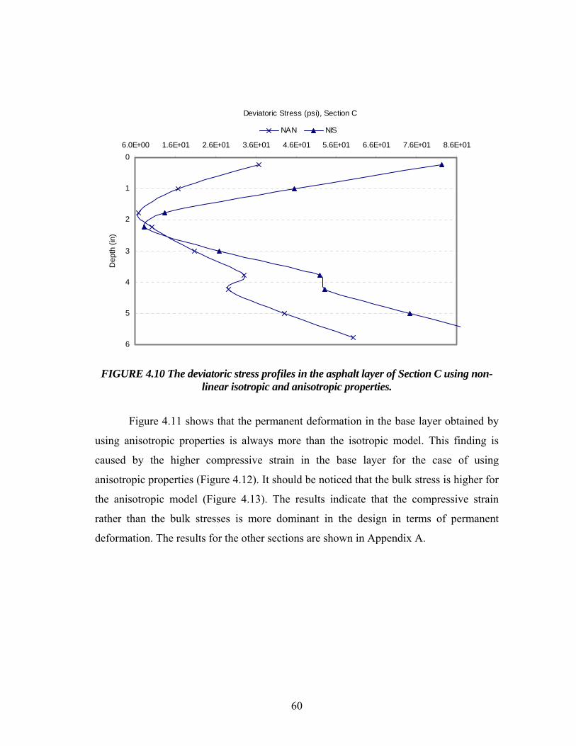
60
0
1
2
3
4
5
6
6.0E+00 1.6E+01 2.6E+01 3.6E+01 4.6E+01 5.6E+01 6.6E+01 7.6E+01 8.6E+01
Deviatoric Stress (psi), Section CD
epth
(in)
NAN NIS
FIGURE 4.10 The deviatoric stress profiles in the asphalt layer of Section C using non-
linear isotropic and anisotropic properties.
Figure 4.11 shows that the permanent deformation in the base layer obtained by
using anisotropic properties is always more than the isotropic model. This finding is
caused by the higher compressive strain in the base layer for the case of using
anisotropic properties (Figure 4.12). It should be noticed that the bulk stress is higher for
the anisotropic model (Figure 4.13). The results indicate that the compressive strain
rather than the bulk stresses is more dominant in the design in terms of permanent
deformation. The results for the other sections are shown in Appendix A.

61
Rutting (Base), Section C
0.03
0.05
0.07
0.09
0.11
0.13
0.15
0.0E+00 5.0E+06 1.0E+07 1.5E+07 2.0E+07 2.5E+07
Number of load repetitions
Per
man
ent D
efor
mat
ion
(in)
lan nan lis nis
FIGURE 4.11 Permanent deformation in the base of Section C using Tseng
and Lytton Model.
0
6
12
18
24
2.0E-04 4.0E-04 6.0E-04 8.0E-04 1.0E-03 1.2E-03 1.4E-03 1.6E-03 1.8E-03
Compressive Strain, Section C
Dep
th (i
n)
NIS NAN
FIGURE 4.12 Compressive strain profiles in the base layer of Section C using non-linear
isotropic and anisotropic properties.

62
0
6
12
18
24
-4.0E+01 -3.0E+01 -2.0E+01 -1.0E+01 0.0E+00
Bulk stress (psi), Section CD
epth
(in)
NIS NAN
FIGURE 4.13 The bulk stress profiles in the base layer of Section C using non-linear
isotropic and anisotropic properties.
0
6
12
18
24
1.0E+00 2.0E+00 3.0E+00 4.0E+00 5.0E+00 6.0E+00 7.0E+00 8.0E+00
Deviatoric Stress (psi), Section C
Dep
th (i
n)
NAN NIS
FIGURE 4.14 The deviatoric stress profiles in the base layer of Section C using
non-linear isotropic and anisotropic properties.

63
The permanent deformation in the subgrade obtained using the isotropic model is
more than that for the anisotropic model. The bulk stress at the top of subgrade is higher
for the anisotropic model as can be seen in Figure 4.13. The deviatoric stress and the
vertical compressive strain for the anisotropic model can be higher or lower than those
of the isotropic. However, the resultant of the effects of the bulk stress, deviatoric stress
and the vertical strain give less permanent deformation using the anisotropic properties.
Figure 4.16 shows the total rutting in section C. The results show that the
permanent deformation for the nonlinear isotropic model is more than that for the
nonlinear anisotropic model.
Rutting (Subgrade), Section C
0.3
0.4
0.5
0.6
0.7
0.8
0.9
1
0.0E+00 5.0E+06 1.0E+07 1.5E+07 2.0E+07 2.5E+07
Number of load repetitions
Per
man
ent D
efor
mat
ion
(in)
lan nan lis nis
FIGURE 4.15 Subgrade permanent deformation in Section C using Tseng
and Lytton Model.

64
Rutting (Total), Section C
0.4
0.5
0.6
0.7
0.8
0.9
1
1.1
1.2
0.0E+00 5.0E+06 1.0E+07 1.5E+07 2.0E+07 2.5E+07
Number of load repetitions
Perm
anen
t Def
orm
atio
n (in
)
lan nan lis nis
FIGURE 4.16 Total permanent deformation in Section C using Tseng and Lytton Model.
The permanent deformation was also calculated in the pavement layers using the
regression equations implemented in the AASHTO 2002 guide. The permanent
deformation for the anisotropic model is more than that for the isotropic model (Figure
4.17).

65
Rutting (HMA), Section C
0.2
0.3
0.4
0.5
0.6
0.7
0.8
0.9
1
0.0E+00 5.0E+06 1.0E+07 1.5E+07 2.0E+07 2.5E+07
Number of load repetitions
Per
man
ent D
efor
mat
ion
(in)
lan nan lis nis
FIGURE 4.17 HMA permanent deformation in Section C using AASHTO 2002 Model.
It can be seen in Figure 4.18 that the permanent deformation in the base layer
obtained using the anisotropic model is always more than the isotropic model. For the
subgrade, the permanent deformation obtained by using isotropic model can be more or
less than that calculated using the anisotropic model depending on the Section And the
material properties. An example of the subgrade permanent deformation is in Figure
4.19. Figure 4.20 shows that the total rutting for the anisotropic model is always more
than that for isotropic model.

66
Rutting (Base), Section C
0.04
0.06
0.08
0.1
0.12
0.14
0.0E+00 5.0E+06 1.0E+07 1.5E+07 2.0E+07 2.5E+07
Number of load repetitions
Per
man
ent D
efor
mat
ion
(in)
lan nan lis nis
FIGURE 4.18 Base permanent deformation in Section C using AASHTO 2002 Model.
Rutting (Subgrade), Section C
0.06
0.08
0.1
0.12
0.14
0.16
0.18
0.2
0.22
0.24
0.0E+00 5.0E+06 1.0E+07 1.5E+07 2.0E+07 2.5E+07
Number of load repetitions
Per
man
ent D
efor
mat
ion
(in)
lan nan lis nis
FIGURE 4.19 Subgrade permanent deformation in Section C
using AASHTO 2002 Model.

67
Rutting (Total), Section C
0.2
0.4
0.6
0.8
1
1.2
1.4
0.0E+00 5.0E+06 1.0E+07 1.5E+07 2.0E+07 2.5E+07
Number of load repetitions
Per
man
ent D
efor
mat
ion
(in)
lan nan lis nis
FIGURE 4.20 Total permanent deformation in Section C using AASHTO 2002 Model.
4.6 Summary of Findings In this chapter the permanent deformation and fatigue cracking were calculated
based on the mechanistic-empirical models used in AASHTO 2002 with isotropic and
anisotropic material properties. The following points summarize the results:
For the base and asphalt layer, the permanent deformation obtained using the
anisotropic model is always more than that with the isotropic model.
The permanent deformation in the subgrade obtained using the isotropic model is
more than that for the anisotropic model when the regression equations from Tseng and
Lytton are used. However, the permanent deformation using the isotropic model can be
more or less than that calculated using the anisotropic model when the regression
equations used in the AASHTO 2002 are used.
The total permanent deformation using the isotropic model can be more or less
than that for anisotropic model when the regression equations from Tseng and Lytton are

68
used. However, the total permanent deformation using the anisotropic model is more
than that calculated using the isotropic model when the AASHTO 2002 equations are
used.
The fatigue life predicted using the nonlinear anisotropic approach is higher than
the life predicted using the nonlinear isotropic approach. This can explain part of the
high shift factor typically found between the laboratory fatigue life calculated using the
isotropic analysis, and field fatigue life. This shift factor is reduced when anisotropic
properties are used.

69
CHAPTER 5 — SENSITIVITY ANALYSIS OF THE AASHTO 2002 DESIGN GUIDE
5.1 Introduction This chapter documents the results of the sensitivity analysis of the AASHTO
2002 Design Guide to the characteristics of the materials used in the unbound pavement
layers. The sensitivity analysis includes two asphalt binder grades, two asphalt layer
thicknesses, three thicknesses for the base layer, five stiffness moduli for the base layer,
three stiffness moduli for the subgrade layer, and three geographic locations representing
different environmental conditions.
5.2 Background on the AASHTO 2002 Design Guide The previous AASHTO guide for the design of pavement for both flexible and
rigid pavement was developed based on the AASHO Road Test experiment about 35
years ago. There are several limitations of this design procedure such as (6):
Pavement rehabilitation design procedures did not exist at the AASHO Road
Test.
The AASHTO road test did not take into accounts the effects of differences in
the climate.
One type of subgrade was used.
There is a big difference between the traffic used in 1950 and the traffic in
modern pavements.
Aging was not addressed because the duration of the road test was just 2 years.
The 2002 design guide is developed based on the mechanistic-empirical design
approach that accounts for climate, aging, and modern vehicle loading. Analysis of the
sensitivity of the AASHTO 2002 flexible pavement design procedure design to the base
properties is presented in this chapter. The material properties used in the analysis are
discussed in the following sections.

70
5.3 Input for the Sensitivity Analysis Three traffic levels are used in the analysis based on the default values in the
AASHTO 2002 guide. The traffic parameters are as follows:
• Two-way average annual daily truck traffic = 1500, 3000, 5000
• Number of lanes in the design direction = 2
• Percent of trucks in design direction = 50%
• Percent of trucks in design lane = 95%
• Optional speed limit = 55 mph
• Design life = 10 years
Traffic growth = 4%
The environmental conditions have a significant effect on the performance of the
flexible pavement. There are two methods to generate the climatic data in the AASHTO
2002 software. The first method uses the data available in the software since the design
guide software includes a database for over 400 cities in the U.S. The next method
provides the following inputs: pavement location latitude and longitude and the elevation
besides the water table depth. Then the climatic data are interpolated to the actual project
location. In this analysis, three locations were selected to represent different climatic
regions: Houston, Texas; Pullman, Washington State; and New York City. The results
presented in this chapter are from the analysis of the Texas site. The results from the
other two sites followed the same trends and, their results are included in Appendix C.
Different pavement sections were analyzed to represent a wide spectrum of
structural designs. The material properties used for the different layers are shown in
Tables 5.2 and 5.3.
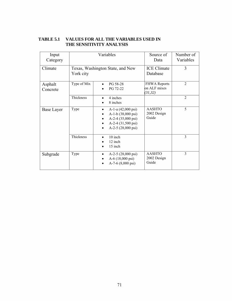
71
TABLE 5.1 VALUES FOR ALL THE VARIABLES USED IN THE SENSITIVITY ANALYSIS
Input Category
Variables Source of Data
Number of Variables
Climate Texas, Washington State, and New York city
ICE Climate Database
3
Type of Mix • PG 58-28 • PG 72-22
FHWA Reports on ALF mixes (31,32)
2 Asphalt Concrete
Thickness • 4 inches • 8 inches
2
Type • A-1-a (42,000 psi) • A-1-b (38,000 psi) • A-2-4 (35,000 psi) • A-2-4 (31,500 psi) • A-2-5 (28,000 psi)
AASHTO 2002 Design Guide
5 Base Layer
Thickness • 10 inch • 12 inch • 15 inch
3
Subgrade Type • A-2-5 (28,000 psi) • A-6 (18,000 psi) • A-7-6 (8,000 psi)
AASHTO 2002 Design Guide
3

72
TABLE 5.2 ASPHALT MIX PROPERTIES Asphalt Mix Property Value
Average Tensile Strength
1600 psi.
Void in Mineral Aggregate 15%
Percent Air Voids 8.5%
Poisson’s ratio 0.35
Thermal conductivity 0.67 BTU/(hr. ft. oF)
Heat capacity asphalt 0.23 BTU/(Ib. oF)
Effective Binder Content 4.8%
TABLE 5.3 UNBOUND LAYER PROPERTIES Modulus (psi) Gradation 42,000 38,000
35,000
31,500 28,000 18000 8,000
PI 1 1 2 2 2 25 40 P200 3 3 20 20 20 80 90 P4 20 40 80 80 80 95 99 D60 8 2 0.1 0.1 0.1 0.01 0.01
5.4 Analysis and Results The sensitivity analysis was conducted based on the main distresses which may
occur in the pavement. The main distresses include roughness, rutting, and fatigue
cracking (top-down and bottom-up cracking). All figures are presented as the percent
change in a certain distress as a function of change in the base material type and
thickness with respect to reference values. The results are shown in Tables 5.4 to 5.15.

73
TABLE 5.4 PERCENT CHANGE IN DIFFERENT TYPES OF DISTRESSES BY CHANGING THE THICKNESS OF THE BASE LAYER USING A-2-5 SUBGRADE (28 KSI) AND PG58-28 BINDER IN THE HMA
Thickness (in)
% Change on Longitudinal Cracking
HMA Base
Base Type
% Change on Rutting Surface Depth=0.5in
% Change on Alligator Cracking
% Change on IRI
4 15 A-1-a(42ksi) 0.000 0.000 0.000 0.000 0.000 4 12 A-1-a -5.198 12.621 20.698 0.000 -1.765 4 10 A-1-a 4.733 13.592 19.535 0.346 1.506 8 15 A-1-a 0.000 0.000 0.000 0.000 0.000 8 12 A-1-a -7.337 -0.121 0.277 -6.218 -4.403 8 10 A-1-a -16.932 1.568 2.774 0.518 0.116 4 15 A-1-b(38ksi) 0.000 0.000 0.000 0.000 0.000 4 12 A-1-b 19.738 5.128 7.283 0.227 0.490 4 10 A-1-b 5.127 9.402 13.386 0.227 0.833 8 15 A-1-b 0.000 0.000 0.000 0.000 0.000 8 12 A-1-b -14.679 -0.932 -0.921 -12.174 -4.363 8 10 A-1-b -32.025 -0.350 -0.132 -11.739 -4.248 4 15 A-2-4(35ksi) 0.000 0.000 0.000 0.000 0.000 4 12 A-2-4 8.181 2.128 4.831 -0.439 -3.941 4 10 A-2-4 4.853 4.255 6.602 0.000 -0.205 8 15 A-2-4 0.000 0.000 0.000 0.000 0.000 8 12 A-2-4 -6.908 -0.568 -0.631 -6.557 -4.530 8 10 A-2-4 -16.665 0.341 0.631 -0.410 0.000 4 15 A-2-4(31.5) 0.000 0.000 0.000 0.000 0.000 4 12 A-2-4 19.695 0.610 1.202 -0.108 -0.454 4 10 A-2-4 5.086 1.220 2.003 -0.108 -0.984 8 15 A-2-4 0.000 0.000 0.000 0.000 0.000 8 12 A-2-4 -14.472 -1.544 -2.169 -14.915 -5.222 8 10 A-2-4 -31.952 -1.544 -2.048 -14.915 -5.222 4 15 A-2-5(28ksi) 0.000 0.000 0.000 0.000 0.000 4 12 A-2-5 19.655 -1.036 -1.106 -0.106 -1.022 4 10 A-2-5 5.026 -2.073 -2.434 -0.213 -2.142 8 15 A-2-5 0.000 0.000 0.000 0.000 0.000 8 12 A-2-5 -14.340 -1.728 -2.448 -15.455 -5.773 8 10 A-2-5 -32.048 -1.836 -2.564 -16.061 -5.773

74
TABLE 5.5 PERCENT CHANGE IN DIFFERENT TYPES OF DISTRESSES BY CHANGING THE THICKNESS OF THE BASE LAYER USING A-6 SUBGRADE (18 KSI) AND PG58-28 BINDER IN THE HMA
Thickness (in)
% Change on Longitudinal Cracking
HMA Base Base Type % Change
on Rutting Surface Depth=0.5in
% Change on Alligator Cracking
% Change on IRI
4 15 A-1-a(42ksi) 0.000 0.000 0.000 0.000 0.000 4 12 A-1-a 3.787 21.359 28.217 0.897 4.281 4 10 A-1-a 5.915 45.631 60.948 1.794 9.400 8 15 A-1-a 0.000 0.000 0.000 0.000 0.000 8 12 A-1-a -9.674 1.548 2.950 0.851 -3.469 8 10 A-1-a 2.316 5.806 9.783 11.489 1.189 4 15 A-1-b(38ksi) 0.000 0.000 0.000 0.000 0.000 4 12 A-1-b 3.885 18.852 25.421 0.768 4.921 4 10 A-1-b 5.994 39.344 52.523 1.427 9.802 8 15 A-1-b 0.000 0.000 0.000 0.000 0.000 8 12 A-1-b 1.652 2.128 3.693 5.645 0.715 8 10 A-1-b 2.806 4.255 7.238 10.887 1.226 4 15 A-2-4(35ksi) 0.000 0.000 0.000 0.000 0.000 4 12 A-2-4 3.810 16.197 20.912 0.541 4.328 4 10 A-2-4 5.873 33.099 43.396 1.081 8.834 8 15 A-2-4 0.000 0.000 0.000 0.000 0.000 8 12 A-2-4 -9.541 0.359 0.826 -1.384 -3.582 8 10 A-2-4 2.373 3.349 5.785 8.304 1.162 4 15 A-2-4(31.5) 0.000 0.000 0.000 0.000 0.000 4 12 A-2-4 3.796 13.095 17.013 0.426 4.111 4 10 A-2-4 5.797 26.190 35.065 0.745 8.571 8 15 A-2-4 0.000 0.000 0.000 0.000 0.000 8 12 A-2-4 1.711 1.174 1.867 4.348 0.598 8 10 A-2-4 2.852 2.230 3.867 7.692 1.097 4 15 A-2-5(28ksi) 0.000 0.000 0.000 0.000 0.000 4 12 A-2-5 3.763 10.553 13.709 0.210 3.999 4 10 A-2-5 5.715 20.603 26.461 0.526 7.336 8 15 A-2-5 0.000 0.000 0.000 0.000 0.000 8 12 A-2-5 -9.402 -0.451 -0.625 -3.390 -3.936 8 10 A-2-5 2.450 1.691 2.875 5.650 1.031

75
TABLE 5.6 PERCENT CHANGE IN DIFFERENT TYPES OF DISTRESSES BY CHANGING THE THICKNESS OF THE BASE LAYER USING A-7-6 SUBGRADE (8 KSI) AND PG58-28 BINDER IN THE HMA
Thickness
(in)
% Change on Longitudinal Cracking
HMA Base
Base Type % Change on Rutting
Surface Depth=0.5in
% Change on Alligator Cracking
% Change on IRI
4 15 A-1-a(42ksi) 0.000 0.000 0.000 0.000 0.000 4 12 A-1-a 4.267 46.829 62.771 1.435 8.488 4 10 A-1-a 6.942 111.382 154.545 2.649 18.557 8 15 A-1-a 0.000 0.000 0.000 0.000 0.000 8 12 A-1-a 1.408 9.600 17.974 11.808 1.326 8 10 A-1-a 2.362 21.600 40.523 22.878 2.653 4 15 A-1-b(38ksi) 0.000 0.000 0.000 0.000 0.000 4 12 A-1-b 4.372 42.674 56.623 1.190 9.303 4 10 A-1-b 7.052 96.658 134.106 2.165 19.361 8 15 A-1-b 0.000 0.000 0.000 0.000 0.000 8 12 A-1-b 1.409 7.394 14.096 10.891 1.483 8 10 A-1-b 2.380 16.197 30.319 20.462 2.880 4 15 A-2-4(35ksi) 0.000 0.000 0.000 0.000 0.000 4 12 A-2-4 4.360 36.601 49.608 0.961 8.762 4 10 A-2-4 6.999 82.482 114.621 1.708 19.118 8 15 A-2-4 0.000 0.000 0.000 0.000 0.000 8 12 A-2-4 1.411 5.591 10.431 9.281 1.463 8 10 A-2-4 2.368 11.981 22.449 17.665 2.926 4 15 A-2-4(31.5) 0.000 0.000 0.000 0.000 0.000 4 12 A-2-4 4.384 31.667 43.232 0.632 9.057 4 10 A-2-4 7.013 70.000 102.020 1.263 18.755 8 15 A-2-4 0.000 0.000 0.000 0.000 0.000 8 12 A-2-4 1.429 4.094 7.632 8.401 1.609 8 10 A-2-4 2.419 8.918 16.438 15.447 3.133 4 15 A-2-5(28ksi) 0.000 0.000 0.000 0.000 0.000 4 12 A-2-5 4.376 27.152 36.476 0.521 8.901 4 10 A-2-5 6.989 57.616 79.289 0.938 18.905 8 15 A-2-5 0.000 0.000 0.000 0.000 0.000 8 12 A-2-5 1.432 2.842 5.326 7.108 1.658 8 10 A-2-5 2.408 6.225 11.684 12.990 3.151

76
TABLE 5.7 PERCENT CHANGE IN DIFFERENT TYPES OF DISTRESSES BY CHANGING THE TYPE OF THE BASE LAYER USING A-2-5 SUBGRADE (28 KSI) AND PG58-28 BINDER IN THE HMA
Thickness (in)
% Change on Longitudinal Cracking
HMA Base Base Type % Change
on Rutting Surface Depth=0.5in
% Change on Alligator Cracking
% Change on IRI
4 10 A-1-a(42ksi) 0.000 0.000 0.000 0.000 0.000 4 10 A-1-b(38ksi) -9.004 9.402 12.062 1.724 5.320 4 10 A-2-4(35ksi) 1.179 25.641 28.794 4.713 24.348 4 10 A-2-4(31.5) -7.591 41.880 48.638 6.092 33.811 4 10 A-2-5(28ksi) -6.773 61.538 71.595 7.701 51.867 8 10 A-1-a 0.000 0.000 0.000 0.000 0.000 8 10 A-1-b -11.152 1.544 2.429 4.639 -3.472 8 10 A-2-4 -0.676 4.869 7.557 25.258 2.199 8 10 A-2-4 -11.736 6.057 9.717 29.381 -1.273 8 10 A-2-5 -11.997 7.957 12.821 42.784 0.116 4 12 A-1-a 0.000 0.000 0.000 0.000 0.000 4 12 A-1-b 14.501 6.034 5.010 2.076 8.457 4 12 A-2-4 15.327 24.138 25.434 4.614 23.679 4 12 A-2-4 16.282 42.241 46.050 6.459 39.006 4 12 A-2-5 17.340 64.655 72.254 8.189 58.721 8 12 A-1-a 0.000 0.000 0.000 0.000 0.000 8 12 A-1-b -0.028 2.657 4.149 11.602 0.970 8 12 A-2-4 -0.537 5.676 8.852 25.967 2.182 8 12 A-2-4 -0.551 7.850 12.310 38.674 3.394 8 12 A-2-5 -0.551 9.903 15.768 54.144 4.848 4 15 A-1-a 0.000 0.000 0.000 0.000 0.000 4 15 A-1-b -9.344 13.592 18.140 1.845 6.023 4 15 A-2-4 1.064 36.893 44.419 5.075 26.480 4 15 A-2-4 -7.901 59.223 74.186 6.574 37.175 4 15 A-2-5 -7.033 87.379 110.233 8.304 57.529 8 15 A-1-a 0.000 0.000 0.000 0.000 0.000 8 15 A-1-b 8.575 3.498 5.409 19.171 0.927 8 15 A-2-4 -0.995 6.152 9.847 26.425 2.317 8 15 A-2-4 7.745 9.409 15.118 52.850 4.287 8 15 A-2-5 7.579 11.701 19.001 70.984 6.373

77
TABLE 5.8 PERCENT CHANGE IN DIFFERENT TYPES OF DISTRESSES BY CHANGING THE TYPE OF THE BASE LAYER USING A-6 SUBGRADE (18 KSI) AND PG58-28 BINDER IN THE HMA
Thickness (in)
% Change on Longitudinal Cracking
HMA Base Base Type % Change
on Rutting Surface Depth=0.5in
% Change on Alligator Cracking
% Change on IRI
4 10 A-1-a(42ksi) 0.000 0.000 0.000 0.000 0.000 4 10 A-1-b(38ksi) 0.998 13.333 14.446 1.762 11.618 4 10 A-2-4(35ksi) 1.820 26.000 27.910 2.974 22.751 4 10 A-2-4(31.5) 2.843 41.333 45.863 4.185 38.483 4 10 A-2-5(28ksi) 4.018 60.000 66.900 5.286 56.999 8 10 A-1-a 0.000 0.000 0.000 0.000 0.000 8 10 A-1-b -10.856 1.585 2.687 4.962 -2.938 8 10 A-2-4 -0.370 5.366 8.628 19.466 2.351 8 10 A-2-4 -11.133 6.220 10.184 22.901 -0.686 8 10 A-2-5 -0.832 10.000 16.407 42.748 5.583 4 12 A-1-a 0.000 0.000 0.000 0.000 0.000 4 12 A-1-b 1.019 16.000 18.134 2.000 11.892 4 12 A-2-4 1.883 32.000 35.387 3.333 23.445 4 12 A-2-4 2.966 52.000 58.627 4.778 39.314 4 12 A-2-5 4.191 76.000 88.380 5.889 59.585 8 12 A-1-a 0.000 0.000 0.000 0.000 0.000 8 12 A-1-b -0.157 3.685 5.882 10.549 1.232 8 12 A-2-4 -0.279 6.607 10.407 20.253 2.259 8 12 A-2-4 -0.454 9.530 15.234 31.646 3.593 8 12 A-2-5 -0.663 12.198 19.910 44.304 5.236 4 15 A-1-a 0.000 0.000 0.000 0.000 0.000 4 15 A-1-b 0.923 18.447 20.767 2.130 11.209 4 15 A-2-4 1.860 37.864 43.567 3.700 23.389 4 15 A-2-4 2.958 63.107 73.815 5.269 39.541 4 15 A-2-5 4.216 93.204 112.415 6.614 60.018 8 15 A-1-a 0.000 0.000 0.000 0.000 0.000 8 15 A-1-b -11.281 3.097 5.124 5.532 -2.973 8 15 A-2-4 -0.425 7.871 12.733 22.979 2.379 8 15 A-2-4 -11.596 9.935 16.460 27.234 -0.595 8 15 A-2-5 -0.961 14.452 24.224 50.638 5.748

78
TABLE 5.9 PERCENT CHANGE IN DIFFERENT TYPES OF DISTRESSES BY CHANGING THE TYPE OF THE BASE LAYER USING A-7-6 SUBGRADE (8 KSI) AND PG58-28 BINDER IN THE HMA
Thickness (in)
% Change on Longitudinal Cracking
HMA Base Base Type % Change
on Rutting Surface Depth=0.5in
% Change on Alligator Cracking
% Change on IRI
4 10 A-1-a(42ksi) 0.000 0.000 0.000 0.000 0.000 4 10 A-1-b(38ksi) 1.234 17.692 20.238 1.505 13.147 4 10 A-2-4(35ksi) 2.290 34.615 39.796 2.473 26.521 4 10 A-2-4(31.5) 3.635 56.923 70.068 3.441 44.647 4 10 A-2-5(28ksi) 5.157 83.077 97.279 4.194 68.240 8 10 A-1-a 0.000 0.000 0.000 0.000 0.000 8 10 A-1-b -0.107 8.553 13.953 9.610 1.550 8 10 A-2-4 -0.260 15.296 25.581 18.018 3.015 8 10 A-2-4 -0.382 22.533 38.372 27.928 4.910 8 10 A-2-5 -0.565 29.112 51.163 38.438 7.149 4 12 A-1-a 0.000 0.000 0.000 0.000 0.000 4 12 A-1-b 1.231 22.924 25.798 1.741 13.229 4 12 A-2-4 2.326 45.072 52.394 2.938 26.245 4 12 A-2-4 3.682 74.972 88.564 4.026 45.164 4 12 A-2-5 5.221 112.625 134.840 5.005 68.385 8 12 A-1-a 0.000 0.000 0.000 0.000 0.000 8 12 A-1-b -0.123 11.314 18.837 10.891 1.483 8 12 A-2-4 -0.262 20.620 34.903 20.462 2.880 8 12 A-2-4 -0.416 29.927 52.355 32.013 4.712 8 12 A-2-5 -0.586 38.686 69.806 44.224 6.981 4 15 A-1-a 0.000 0.000 0.000 0.000 0.000 4 15 A-1-b 1.129 26.504 30.736 1.987 12.384 4 15 A-2-4 2.235 55.935 65.801 3.422 25.926 4 15 A-2-4 3.566 95.122 114.286 4.857 44.406 4 15 A-2-5 5.111 145.528 180.087 5.960 67.747 8 15 A-1-a 0.000 0.000 0.000 0.000 0.000 8 15 A-1-b -0.125 13.600 22.876 11.808 1.326 8 15 A-2-4 -0.266 25.200 44.118 23.247 2.741 8 15 A-2-4 -0.438 36.800 66.993 36.162 4.421 8 15 A-2-5 -0.610 47.800 90.196 50.554 6.631

79
TABLE 5.10 PERCENT CHANGE IN DIFFERENT TYPES OF DISTRESSES BY CHANGING THE THICKNESS OF THE BASE LAYER USING A-2-5 SUBGRADE (28 KSI) AND PG76-22 BINDER IN THE HMA
Thickness (in)
% Change on Longitudinal Cracking
HMA Base Base Type % Change
on Rutting Surface Depth=0.5in
% Change on Alligator Cracking
% Change on IRI
4 15 A-1-a(42ksi) 0.000 0.000 0.000 0.000 0.000 4 10 A-1-a 6.034 13.497 17.587 0.324 2.641 8 15 A-1-a 0.000 0.000 0.000 0.000 0.000 8 10 A-1-a -22.506 0.921 1.536 1.587 0.117 4 15 A-2-4(35) 0.000 0.000 0.000 0.000 0.000 4 10 A-2-4 5.953 4.545 5.455 0.000 0.000 8 15 A-2-4 0.000 0.000 0.000 0.000 0.000 8 10 A-2-4 -22.194 0.221 0.361 0.338 0.000 4 15 A-2-5(28ksi) 0.000 0.000 0.000 0.000 0.000 4 10 A-2-5 5.740 -1.718 -1.961 -0.104 -2.161 8 15 A-2-5 0.000 0.000 0.000 0.000 0.000 8 10 A-2-5 -22.734 -0.108 -0.345 -1.729 -0.333
TABLE 5.11 PERCENT CHANGE IN DIFFERENT TYPES OF DISTRESSES BY CHANGING THE THICKNESS OF THE BASE LAYER USING A-6 SUBGRADE (18 KSI) AND PG76-22 BINDER IN THE HMA
Thickness (in)
% Change on Longitudinal Cracking
HMA Base Base Type % Change
on Rutting Surface Depth=0.5in
% Change on Alligator Cracking
% Change on IRI
4 15 A-2-4(35) 0.000 0.000 0.000 0.000 0.000 4 10 A-2-4 7.032 27.111 35.714 0.521 10.486 8 15 A-2-4 0.000 0.000 0.000 0.000 0.000 8 10 A-2-4 3.440 1.769 3.075 7.649 1.552 4 15 A-2-5(28ksi) 0.000 0.000 0.000 0.000 0.000 4 10 A-2-5 6.801 16.225 22.013 0.309 8.531 8 15 A-2-5 0.000 0.000 0.000 0.000 0.000 8 10 A-2-5 3.447 0.904 1.498 5.172 1.317 4 15 A-1-a(42ksi) 0.000 0.000 0.000 0.000 0.000 4 10 A-1-a 7.243 39.053 50.498 1.060 11.601 8 15 A-1-a 0.000 0.000 0.000 0.000 0.000 8 10 A-1-a 3.503 2.981 5.225 10.458 1.690

80
TABLE 5.12 PERCENT CHANGE IN DIFFERENT TYPES OF DISTRESSES BY CHANGING THE THICKNESS OF THE BASE LAYER USING A-7-6 SUBGRADE (8 KSI) AND PG76-22 BINDER IN THE HMA
Thickness (in)
% Change on Longitudinal Cracking
HMA Base Base Type % Change
on Rutting Surface Depth=0.5in
% Change on Alligator Cracking
% Change on IRI
4 15 A-1-a(42ksi) 0.000 0.000 0.000 0.000 0.000 4 12 A-1-a 5.803 38.532 51.770 0.735 11.117 4 10 A-1-a 9.417 86.239 121.239 1.364 24.099 8 15 A-1-a 0.000 0.000 0.000 0.000 0.000 8 12 A-1-a 2.024 3.711 7.365 9.896 2.101 8 10 A-1-a 3.388 10.575 19.830 18.490 4.202 4 15 A-2-4(35ksi) 0.000 0.000 0.000 0.000 0.000 4 12 A-2-4 5.710 29.630 39.082 0.517 11.138 4 10 A-2-4 9.244 62.963 87.761 0.826 23.715 8 15 A-2-4 0.000 0.000 0.000 0.000 0.000 8 12 A-2-4 1.985 1.875 3.863 7.675 2.195 8 10 A-2-4 3.349 5.625 10.730 14.221 4.309 4 15 A-2-5(28ksi) 0.000 0.000 0.000 0.000 0.000 4 12 A-2-5 5.591 20.921 28.696 0.306 10.525 4 10 A-2-5 8.974 43.096 60.870 0.511 21.769 8 15 A-2-5 0.000 0.000 0.000 0.000 0.000 8 12 A-2-5 1.966 0.822 1.730 5.709 2.260 8 10 A-2-5 3.312 2.740 5.363 10.236 4.287 4 15 A-1-b(38ksi) 0.000 0.000 0.000 0.000 0.000 4 12 A-1-b 5.830 35.075 46.287 0.624 12.033 4 10 A-1-b 9.426 75.373 103.800 1.145 24.610 8 15 A-1-b 0.000 0.000 0.000 0.000 0.000 8 12 A-1-b 2.005 2.862 5.825 8.916 2.231 8 10 A-1-b 3.368 7.912 14.806 16.386 4.298
4 15 A-2-4(31.5ksi) 0.000 0.000 0.000 0.000 0.000
4 12 A-2-4 5.670 24.873 34.361 0.308 11.402 4 10 A-2-4 9.138 52.284 74.009 0.616 22.804 8 15 A-2-4 0.000 0.000 0.000 0.000 0.000 8 12 A-2-4 1.986 1.312 2.682 6.526 2.231 8 10 A-2-4 3.331 4.082 7.854 12.211 4.303

81
TABLE 5.13 PERCENT CHANGE IN DIFFERENT TYPES OF DISTRESSES BY CHANGING THE TYPE OF THE BASE LAYER USING A-2-5 SUBGRADE (28 KSI) AND PG76-22 BINDER IN THE HMA
Thickness (in)
% Change on Longitudinal Cracking
HMA Base Base Type % Change
on Rutting Surface Depth=0.5in
% Change on Alligator Cracking
% Change on IRI
4 10 A-1-a(42ksi) 0.000 0.000 0.000 0.000 0.000 4 10 A-2-4(35) 1.284 24.324 26.638 2.153 24.175 4 10 A-2-5(28ksi) 3.075 54.595 63.755 3.767 57.521 8 10 A-1-a 0.000 0.000 0.000 0.000 0.000
8 10 A-2-4 -0.572 3.307 5.170 16.016 2.222
8 10 A-2-5 -0.990 5.929 9.206 33.203 4.912 4 15 A-1-a 0.000 0.000 0.000 0.000 0.000 4 15 A-2-4 1.361 34.969 41.207 2.484 27.455 4 15 A-2-5 3.361 78.528 96.406 4.212 65.253 8 15 A-1-a 0.000 0.000 0.000 0.000 0.000 8 15 A-2-4 -0.972 4.028 6.402 17.460 2.342 8 15 A-2-5 -0.699 7.020 11.268 37.698 5.386
TABLE 5.14 PERCENT CHANGE IN DIFFERENT TYPES OF DISTRESSES BY CHANGING THE TYPE OF THE BASE LAYER USING A-6 SUBGRADE (18 KSI) AND PG76-22 BINDER IN THE HMA
Thickness (in)
% Change on Longitudinal Cracking
HMA Base Base Type % Change
on Rutting Surface Depth=0.5in
% Change on Alligator Cracking
% Change on IRI
4 10 A-1-a(42ksi) 0.000 0.000 0.000 0.000 0.000 4 10 A-2-4(35) 1.862 21.702 25.620 1.259 23.395 4 10 A-2-5(28ksi) 4.123 49.362 60.331 2.308 57.185 8 10 A-1-a 0.000 0.000 0.000 0.000 0.000 8 10 A-2-4 -0.198 4.101 6.345 12.426 2.346 8 10 A-2-5 -0.396 7.720 12.138 26.331 5.279 4 15 A-1-a 0.000 0.000 0.000 0.000 0.000 4 15 A-2-4 2.062 33.136 39.303 1.803 24.640 4 15 A-2-5 4.554 78.698 97.761 3.075 61.631 8 15 A-1-a 0.000 0.000 0.000 0.000 0.000 8 15 A-2-4 -0.136 5.342 8.563 15.359 2.485 8 15 A-2-5 -0.341 9.938 16.255 32.680 5.666

82
TABLE 5.15 PERCENT CHANGE IN DIFFERENT TYPES OF DISTRESSES BY CHANGING THE TYPE OF THE BASE LAYER USING A-7-6 SUBGRADE (8 KSI) AND PG76-22 BINDER IN THE HMA
Thickness (in) % Change on Longitudinal Cracking
HMA Base Base Type % Change
on Rutting Surface Depth=0.5in
% Change on Alligator Cracking
% Change on IRI
4 10 A-1-a(42ksi) 0.000 0.000 0.000 0.000 0.000 4 10 A-1-b(38ksi) 1.343 15.764 18.000 0.621 13.447
4 10 A-2-4 (35.0ksi) 2.522 30.049 35.000 1.035 27.409
4 10 A-2-4(31.5 ksi) 3.933 47.783 58.000 1.449 44.831
4 10 A-2-5(28ksi) 5.509 68.473 85.000 1.863 67.257 8 10 A-1-a 0.000 0.000 0.000 0.000 0.000 8 10 A-1-b -0.060 7.550 11.820 6.154 1.774 8 10 A-2-4 -0.120 13.423 21.986 11.209 3.468 8 10 A-2-4 -0.200 19.799 33.097 17.143 5.565 8 10 A-2-5 -0.280 25.839 43.972 23.077 7.903 4 12 A-1-a 0.000 0.000 0.000 0.000 0.000 4 12 A-1-b 1.361 19.868 23.469 0.729 13.914 4 12 A-2-4 2.594 39.073 45.773 1.354 27.829 4 12 A-2-4 4.067 62.914 77.843 1.771 61.753 4 12 A-2-5 5.726 91.391 115.743 2.292 69.549 8 12 A-1-a 0.000 0.000 0.000 0.000 0.000 8 12 A-1-b -0.061 9.302 15.040 7.109 1.811 8 12 A-2-4 -0.121 16.637 27.704 13.033 3.457 8 12 A-2-4 -0.182 24.329 41.425 19.905 5.597 8 12 A-2-5 -0.263 31.664 55.145 27.251 7.984 4 15 A-1-a 0.000 0.000 0.000 0.000 0.000 4 15 A-1-b 1.335 22.936 28.097 0.839 12.982 4 15 A-2-4 2.684 48.624 59.071 1.574 27.805 4 15 A-2-4 4.199 80.734 100.885 2.204 46.358 4 15 A-2-5 5.938 119.266 154.425 2.728 70.457 8 15 A-1-a 0.000 0.000 0.000 0.000 0.000 8 15 A-1-b -0.041 10.204 16.714 8.073 1.681 8 15 A-2-4 -0.083 18.738 32.011 15.365 3.361 8 15 A-2-4 -0.145 27.273 47.875 23.698 5.462 8 15 A-2-5 -0.207 35.436 63.739 32.292 7.815

83
5.4.1 Roughness Smoothness can be defined as “the variation in surface elevation that induces
vibrations in traversing vehicles” (6). Rough roads not only lead to user discomfort but
also to increased travel times and higher vehicle operating costs. The IRI is one of the
ways to measure the smoothness. The designer has to choose the terminal IRI values that
should not be exceeded at the design level of reliability. Typical values range from 63 to
1260 in/mi (6). Figure 5.1 shows the change in the IRI as the base modulus changes
from 42,000 psi to 28,000 psi for different thicknesses for the base layer. The y axis
represents the percentage change in the IRI as the base modulus changes from 42,000 psi
to another value where the data point is plotted. It can be seen that the IRI value
increases as the base modulus gets smaller irrespective of the base thickness. As can be
seen in Figure 5.2, the effect of the change in the base modulus on IRI becomes smaller
as the HMA thickness becomes larger. The influence of base thickness on IRI increases
as the HMA thickness decreases and as the subgrade stiffness decreases, (Figure 5.3).
These results are almost the same for PG 58-22 and PG 72-22 mixes.
PG58-28 , 8in HMASubgrade Modulus = 8,000psi
0
1
2
3
4
5
6
7
8
2.6E+04 3.0E+04 3.4E+04 3.8E+04 4.2E+04
Base Modulus (psi)
% C
hang
e on
IRI
10 in 12 in 15 in
FIGURE 5.1 Percent change in IRI for different thicknesses of the base layer at 8in
HMA and 8 ksi subgrade.

84
PG58-28, 12 in UAB
0
10
20
30
40
50
60
70
80
2.6E+04 3.0E+04 3.4E+04 3.8E+04 4.2E+04
Base Modulus (Psi)
% C
hang
e on
IRI
4in HMA,8Ksi Subgrade 4in HMA,18Ksi Subgrade 8in HMA,8Ksi Subgrade
FIGURE 5.2 Percent change in IRI at two different thicknesses of HMA and at two types
of subgrade by changing the base modulus. PG58-28 , A-1-b (38Ksi)
0
4
8
12
16
20
9 10 11 12 13 14 15 16
Base Thickness (in)
% C
hang
e on
IRI
4in HMA, 18Ksi Subgrade 8in HMA, 8Ksi Subgrade8in HMA, 18Ksi Subgrade 4in HMA, 8Ksi Subgrade
FIGURE 5.3 Percent change in IRI at two different thicknesses of HMA and at two types
of subgrade by changing the base thickness.

85
5.4.2 Surface-Down Fatigue Cracking (Longitudinal Cracking) Surface-down fatigue cracking is defined as longitudinal cracking at the edge of
the wheel paths. Surface-down cracking can cause loss of smoothness and permits water
infiltration into the underlying pavement layers which can be a reason for structural
failure of the pavement. The performance criterion for Surface-down fatigue cracking is
defined as the maximum allowable length of longitudinal cracking per mile of pavement
that is permitted to occur at the end of the design life. Typical values of allowable
Surface-down fatigue cracking are on the order of 500 to 2000 ft/mi of pavement (6).
The longitudinal cracking is calculated by considering the critical tensile stress at the
surface and at 0.5 inch below the surface.
The base type has significant influence on longitudinal cracking as shown in
Figure 5.4. Longitudinal cracking increases up to 190% when the base modulus
decreases from 42,000 psi to 28,000 psi in a pavement with PG 58-28 binder, 8000 psi
subgrade, and 15 in. base thickness. The influence of base modulus on longitudinal
cracking decreases as the base thickness decreases (Figure 5.4), and as the HMA
thickness increases (Figure 5.4 and 5.5). Also, comparing Figures 5.4 and 5.5 with
Figures 5.6 and 5.7 reveals that the influence of the base modulus on fatigue cracking
decreases as the subgrade modulus increases. Figures 5.9 to 5.11 show clearly that the
longitudinal cracking increases as the base thickness decreases. The relationship between
base thickness and longitudinal cracking is sensitive to subgrade stiffness and HMA
thickness as shown in Figures 5.9 to 5.12.

86
PG58-28 , 4in HMASubgrade Modulus = 8,000psi`
0
20
40
60
80
100
120
140
160
180
200
2.6E+04 3.0E+04 3.4E+04 3.8E+04 4.2E+04
Base Modulus (psi)
% C
hang
e on
Lon
gitu
dina
l Cra
ckin
g
10in (Surface) 12in (Surface) 15in (Surface)
10in (Depth) 12in (Depth) 15in (Depth)
FIGURE 5.4 Percent change in longitudinal cracking for different thickness of the base
layer at 4in HMA and 8 ksi subgrade. PG58-28 , 8in HMA
Subgrade Modulus = 8,000psi
0
10
20
30
40
50
60
70
80
90
100
2.6E+04 3.0E+04 3.4E+04 3.8E+04 4.2E+04
Base Modulus (psi)
% C
hang
e on
Lon
gitu
dina
l Cra
ckin
g
10in (Surface) 12in (Surface) 15in (Surface)10in (Depth=0.5in) 12in (Depth=0.5in) 15in (Depth=0.5in)
FIGURE 5.5 Percent change in longitudinal cracking for different thickness of the base
layer at 8 in. HMA and 8 ksi subgrade.

87
PG58-28 , 4in HMASubgrade Modulus = 18,000psi
0
20
40
60
80
100
120
2.6E+04 3.0E+04 3.4E+04 3.8E+04 4.2E+04
Base Modulus (psi)
% C
hang
e on
Lon
gitu
dina
l Cra
ckin
g
10in (Surface) 12in (Surface) 15in (Surface)
10in (Depth=0.5in) 12in (Depth=0.5in) 15in (Depth=0.5in)
FIGURE 5.6 Percent change in longitudinal cracking for different thickness of the base
layer at 4 in. HMA and 18 ksi subgrade.
PG58-28 , 8in HMASubgrade Modulus = 18,000psi
0
5
10
15
20
25
30
2.6E+04 3.0E+04 3.4E+04 3.8E+04 4.2E+04
Base Modulus (psi)
% C
hang
e on
Lon
gitu
dina
l Cra
ckin
g
10in (Surface) 12in (Surface) 15in (Surface)
10in (Depth=0.5in) 12in (Depth=0.5in) 15in (Depth=0.5in)
FIGURE 5.7 Percent change in longitudinal cracking for different thickness of the base
layer at 8 in. HMA and 18 ksi subgrade.

88
PG58-28 , 8in HMA
Subgrade Modulus = 28,000psi
0
2
4
6
8
10
12
14
16
18
20
2.6E+04 3.0E+04 3.4E+04 3.8E+04 4.2E+04
Base Modulus (psi)
% C
hang
e on
Lon
gitu
dina
l Cra
ckin
g10in (Surface) 12in (Surface) 15in (Surface)
10in (Depth=0.5in) 12in (Depth=0.5in) 15in (Depth=0.5in)
FIGURE 5.8 Percent change in longitudinal cracking for different thickness of the base
layer at 8 in. HMA and 28 ksi subgrade. PG58-28 , 4in HMA
Subgrade Modulus = 8,000psi`
0
40
80
120
160
9 10 11 12 13 14 15 16
Base Thickness (in)
% C
hang
e on
Long
itudi
nal C
rack
ing
A-1-a (42Ksi) Surface A-2-4 (35Ksi) Surface A-2-5 (28Ksi) Surface
A-1-a (42Ksi) Depth A-2-4 (35Ksi) Depth A-2-5 (28Ksi) Depth
FIGURE 5.9 Percent change in longitudinal cracking for different types of the base layer
at 4 in. HMA and 8 ksi subgrade.
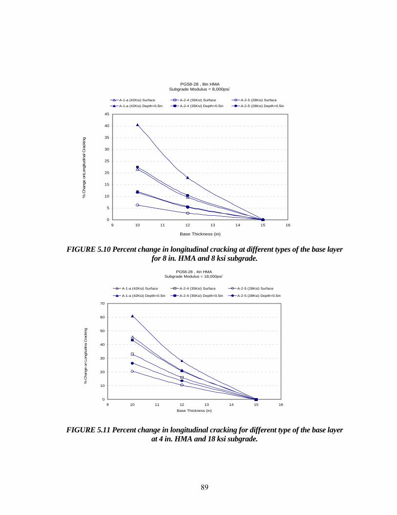
89
PG58-28 , 8in HMASubgrade Modulus = 8,000psi`
0
5
10
15
20
25
30
35
40
45
9 10 11 12 13 14 15 16
Base Thickness (in)
% C
hang
e on
Long
itudi
nal C
rack
ing
A-1-a (42Ksi) Surface A-2-4 (35Ksi) Surface A-2-5 (28Ksi) Surface
A-1-a (42Ksi) Depth=0.5in A-2-4 (35Ksi) Depth=0.5in A-2-5 (28Ksi) Depth=0.5in
FIGURE 5.10 Percent change in longitudinal cracking at different types of the base layer
for 8 in. HMA and 8 ksi subgrade. PG58-28 , 4in HMA
Subgrade Modulus = 18,000psi`
0
10
20
30
40
50
60
70
9 10 11 12 13 14 15 16
Base Thickness (in)
% C
hang
e on
Lon
gitu
dina
Cra
ckin
g
A-1-a (42Ksi) Surface A-2-4 (35Ksi) Surface A-2-5 (28Ksi) Surface
A-1-a (42Ksi) Depth=0.5in A-2-4 (35Ksi) Depth=0.5in A-2-5 (28Ksi) Depth=0.5in
FIGURE 5.11 Percent change in longitudinal cracking for different type of the base layer
at 4 in. HMA and 18 ksi subgrade.

90
PG58-28 , 8in HMASubgrade Modulus = 18,000psi`
-1
1
3
5
7
9
9 10 11 12 13 14 15 16
Base Thickness (in)
% C
hang
e on
Lon
gitu
dina
Cra
ckin
g
A-1-a (42Ksi) Surface A-2-4 (35Ksi) Surface A-2-5 (28Ksi) Surface
A-1-a (42Ksi) Depth=0.5in A-2-4 (35Ksi) Depth=0.5in A-2-5 (28Ksi) Depth=0.5in
FIGURE 5.12 Percent change in longitudinal cracking for different types of the base
layer at 8 in. HMA and 18 ksi subgrade.
5.4.3 Bottom-Up Fatigue Cracking This type of cracking starts from the bottom of the layer and propagates to the
top so the critical fatigue depth location is at the bottom of the asphalt layer. Bottom-up
fatigue cracking appears as alligator cracking within the wheel paths (6). Bottom-up
cracking has an effect on the smoothness which can cause loss of smoothness and can
permit water infiltration into the underlying pavement layers that can cause structural
failure of the pavement. The performance criterion for bottom-up fatigue cracking is
defined as the percentage of the cracking per total lane area that may occur over the
design period. Typical values of allowable Surface-down fatigue cracking are on the
order of 25 to 100% of pavement (6). The alligator cracking is calculated by considering
the critical tensile stress at the bottom of the pavement.
The base type has significant influence on alligator cracking as shown in Figure
5.14. Alligator cracking increases by about 50% when the base modulus decreases from

91
42,000 psi to 28,000 psi in a pavement with PG 58-28 binder, 8000 psi subgrade, and
15 in. base thickness. The influence of base modulus on alligator cracking decreases as
the base thickness decreases (Figure 5.14) and as the HMA thickness decreases (Figures
5.13 and 5.14). Also, comparing Figures 5.13 and 5.14 with Figures 5.15 and 5.16
indicates that the influence of the base modulus on fatigue cracking is the same
irrespective of the subgrade type. Figures 5.18 and 5.20 show clearly that the base
thickness has significant influence on alligator cracking. The relationship between base
thickness and alligator cracking depends on subgrade stiffness and HMA thickness as
shown in Figures 5.17 to 5.20.
PG58-28 , 4in HMASubgrade Modulus = 8,000psi
0
1
2
3
4
5
6
7
2.6E+04 3.0E+04 3.4E+04 3.8E+04 4.2E+04
Base Modulus (psi)
% C
hang
e on
Alli
gato
r Cra
ckin
g
10in 12in 15in
FIGURE 5.13 Percent change in alligator cracking for different thicknesses of the base
layer at 4 in. HMA and 8 ksi subgrade.
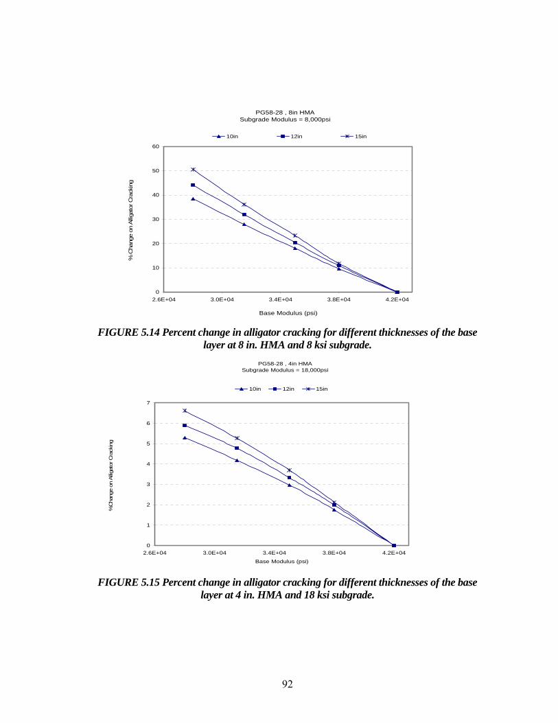
92
PG58-28 , 8in HMASubgrade Modulus = 8,000psi
0
10
20
30
40
50
60
2.6E+04 3.0E+04 3.4E+04 3.8E+04 4.2E+04
Base Modulus (psi)
% C
hang
e on
Alli
gato
r Cra
ckin
g10in 12in 15in
FIGURE 5.14 Percent change in alligator cracking for different thicknesses of the base
layer at 8 in. HMA and 8 ksi subgrade. PG58-28 , 4in HMA
Subgrade Modulus = 18,000psi
0
1
2
3
4
5
6
7
2.6E+04 3.0E+04 3.4E+04 3.8E+04 4.2E+04
Base Modulus (psi)
%C
hang
e on
Allig
ator
Cra
ckin
g
10in 12in 15in
FIGURE 5.15 Percent change in alligator cracking for different thicknesses of the base
layer at 4 in. HMA and 18 ksi subgrade.

93
PG58-28 , 8in HMA
Subgrade Modulus = 18,000psi
0
10
20
30
40
50
60
2.6E+04 3.0E+04 3.4E+04 3.8E+04 4.2E+04
Base Modulus (psi)
% C
hang
e on
Alli
gato
r Cra
ckin
g
10in 12in 15in
FIGURE 5.16 Percent change in alligator cracking for different thicknesses of the base
layer at 8 in. HMA and 18 ksi subgrade. PG58-28 , 4in HMA
Subgrade Modulus = 8,000psi`
0
0.5
1
1.5
2
2.5
3
9 10 11 12 13 14 15 16
Base Thickness (in)
% C
hang
e A
lliga
tor C
rack
ing
A-1-a (42Ksi) A-1-b (38Ksi) A-2-4 (35Ksi)A-2-4 (31.5Ksi) A-2-5 (28Ksi)
FIGURE 5.17 Percent change in alligator cracking for different types of the base layer at
4 in HMA and 8 ksi subgrade.

94
PG58-28 , 8in HMA
Subgrade Modulus = 8,000psi`
0
5
10
15
20
25
9 10 11 12 13 14 15 16
Base Thickness (in)
% C
hang
e A
lligat
or C
rack
ing
A-1-a (42Ksi) A-1-b (38Ksi) A-2-4 (35Ksi) A-2-4 (31.5Ksi) A-2-5 (28Ksi)
FIGURE 5.18 Percent change in alligator cracking for different types of the base layer at
8 in. HMA and 8 ksi subgrade. PG58-28 , 4in HMA
Subgrade Modulus = 18,000psi`
0
0.2
0.4
0.6
0.8
1
1.2
1.4
1.6
1.8
2
9 10 11 12 13 14 15 16
Base Thickness (in)
% C
hang
e A
lliga
tor C
rack
ing
A-1-a (42Ksi) A-1-b (38Ksi) A-2-4 (35Ksi) A-2-4 (31.5Ksi) A-2-5 (28Ksi)
FIGURE 5.19 Percent change in alligator cracking for different types of the base layer at
4 in. HMA and 18 ksi subgrade.

95
PG58-28 , 8in HMASubgrade Modulus = 18,000psi`
-4
-2
0
2
4
6
8
10
12
9 10 11 12 13 14 15 16
Base Thickness (in)
% C
hang
e A
lligat
or C
rack
ing
A-1-a (42Ksi) A-1-b (38Ksi) A-2-4 (35Ksi) A-2-4 (31.5Ksi) A-2-5 (28Ksi)
FIGURE 5.20 Percent change in alligator cracking for different types of the base layer at
8 in. HMA and 18 ksi subgrade.
5.4.4 Permanent Deformation Permanent deformation is one of the most important types of distresses in
flexible pavements. Water can accumulate in traffic lanes and reduce skid resistance of
the surface and cause unsafe traffic conditions. In AASHTO 2002 design guide, the
permanent deformation is calculated at the mid-depth of each sublayer within the
pavement so that the overall permanent deformation is the summation of the permanent
deformation for all the layers. The performance criterion for total permanent
deformation is defined in terms of the maximum rut depth in the wheel path. A typical
maximum rut depth for total permanent deformation is about 3 in (6).

96
All the results from the permanent deformation analysis show that the base
properties have almost no influence on permanent deformation (Figures 5.21 to 5.26).
This is a surprising result given that the main function of the base layer is the
distribution of applied loads to reduce permanent deformation. The analysis in Chapter 4
of this thesis showed that the permanent deformation models are sensitive to the base
properties. This finding indicates that the implementation of these models in the
AASHTO 2002 should be carefully reviewed.
PG58-28 , 4in HMASubgrade Modulus = 8,000psi
0
1
2
3
4
5
6
2.60E+04 3.00E+04 3.40E+04 3.80E+04 4.20E+04
Base Modulus (psi)
% C
hang
e on
Rut
ting
10in 12in 15in
FIGURE 5.21 Percent change in rutting for different thicknesses of the base layer at 4 in.
HMA and 8 ksi subgrade.

97
PG58-28 , 8in HMASubgrade Modulus = 8,000psi
-0.7
-0.6
-0.5
-0.4
-0.3
-0.2
-0.1
0
2.6E+04 3.0E+04 3.4E+04 3.8E+04 4.2E+04
Base modulus (psi)
% C
hang
e on
Rut
ting
10in 12in 15in
FIGURE 5.22 Percent change on rutting for different thicknesses of the base layer at 8 in.
HMA and 8ksi subgrade. PG58-28 , 4in HMA
Subgrade Modulus = 18,000psi
0
0.5
1
1.5
2
2.5
3
3.5
4
4.5
2.6E+04 3.0E+04 3.4E+04 3.8E+04 4.2E+04
Base Modulus (psi)
% C
hang
e on
Rut
ting
10in 12in 15in
FIGURE 5.23 Percent change on rutting for different thicknesses of the base layer at 4 in.
HMA and 18 ksi subgrade.

98
PG58-28 , 4in HMASubgrade Modulus = 8,000psi`
0
1
2
3
4
5
6
7
8
9 10 11 12 13 14 15 16
Base Thickness (in)
% C
hang
e on
Rut
ting
A-1-a (42Ksi) A-1-b (38Ksi) A-2-4 (35Ksi) A-2-4 (31.5Ksi) A-2-5 (28Ksi)
FIGURE 5.24 Percent change on rutting for different types of the base layer at 4 in.
HMA and 8 ksi subgrade.
PG58-28 , 8in HMASubgrade Modulus = 8,000psi`
0
0.5
1
1.5
2
2.5
9 10 11 12 13 14 15 16
Base Thickness (in)
% C
hang
e on
Rut
ting
A-1-a (42Ksi) A-1-b (38Ksi) A-2-4 (35Ksi) A-2-4 (31.5Ksi) A-2-5 (28Ksi)
FIGURE 5.25 Percent change on rutting for different types of the base layer at 8 in.
HMA and 8 ksi subgrade.

99
PG58-28 , 4in HMA
Subgrade Modulus = 18,000psi`
0
1
2
3
4
5
6
7
9 10 11 12 13 14 15 16
Base Thickness(in)
% C
hang
e on
Rut
ting
A-1-a (42Ksi) A-1-b (38Ksi) A-2-4 (35Ksi) A-2-4 (31.5Ksi) A-2-5 (28Ksi)
FIGURE 5.26 Percent change on rutting for different types of the base layer at 4 in.
HMA and 18ksi subgrade.
5.5 Summary of Findings The sensitivity analysis results show that the base modulus and thickness have
significant influence on the international roughness index and the longitudinal cracking.
The influence of base properties on alligator cracking is about half of the influence of
base properties on longitudinal cracking. All the results show that the base properties
have almost no influence on permanent deformation. These findings are applicable to the
three climatic zones, the two asphalt binder grades, and three traffic levels used in this
study.
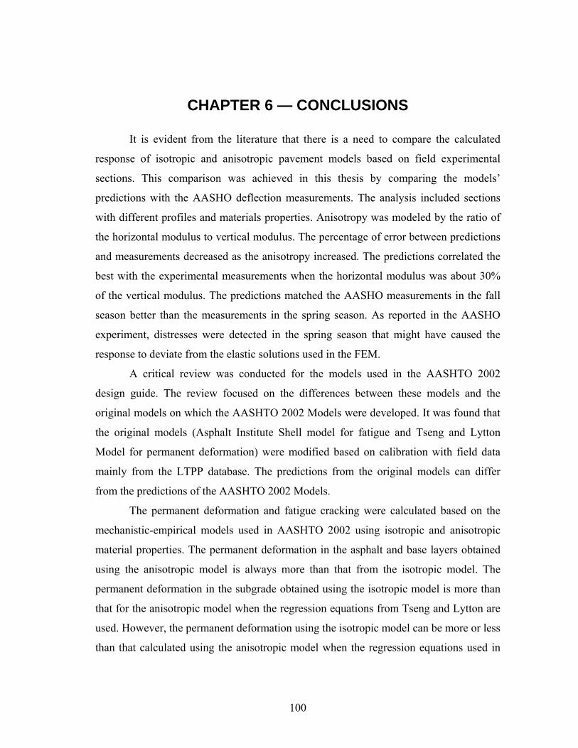
100
CHAPTER 6 — CONCLUSIONS
It is evident from the literature that there is a need to compare the calculated
response of isotropic and anisotropic pavement models based on field experimental
sections. This comparison was achieved in this thesis by comparing the models’
predictions with the AASHO deflection measurements. The analysis included sections
with different profiles and materials properties. Anisotropy was modeled by the ratio of
the horizontal modulus to vertical modulus. The percentage of error between predictions
and measurements decreased as the anisotropy increased. The predictions correlated the
best with the experimental measurements when the horizontal modulus was about 30%
of the vertical modulus. The predictions matched the AASHO measurements in the fall
season better than the measurements in the spring season. As reported in the AASHO
experiment, distresses were detected in the spring season that might have caused the
response to deviate from the elastic solutions used in the FEM.
A critical review was conducted for the models used in the AASHTO 2002
design guide. The review focused on the differences between these models and the
original models on which the AASHTO 2002 Models were developed. It was found that
the original models (Asphalt Institute Shell model for fatigue and Tseng and Lytton
Model for permanent deformation) were modified based on calibration with field data
mainly from the LTPP database. The predictions from the original models can differ
from the predictions of the AASHTO 2002 Models.
The permanent deformation and fatigue cracking were calculated based on the
mechanistic-empirical models used in AASHTO 2002 using isotropic and anisotropic
material properties. The permanent deformation in the asphalt and base layers obtained
using the anisotropic model is always more than that from the isotropic model. The
permanent deformation in the subgrade obtained using the isotropic model is more than
that for the anisotropic model when the regression equations from Tseng and Lytton are
used. However, the permanent deformation using the isotropic model can be more or less
than that calculated using the anisotropic model when the regression equations used in

101
the AASHTO 2002 are used. The total permanent deformation using the isotropic model
can be more or less than that for the anisotropic model when the regression equations
from Tseng and Lytton are used. However, the total permanent deformation using the
anisotropic model is more than that calculated using the isotropic model when the
AASHTO 2002 equations are used.
The fatigue life predicted using the nonlinear anisotropic approach is higher than
the life predicted using the nonlinear isotropic approach. This discrepancy can explain
the high shift factor typically found between the laboratory fatigue life calculated using
the isotropic analysis, and the field fatigue life. This shift factor can be reduced when
anisotropic properties are used.
The sensitivity analysis of the AASHTO 2002 Model shows that the base
modulus and thickness have significant influence on the international roughness index
and the longitudinal cracking. The influence of base properties on alligator cracking is
about half of the influence of base properties on longitudinal cracking. Surprisingly, all
the results show that the base properties have almost no influence on permanent
deformation. These findings are applicable to all the material properties, pavement
profiles, and environmental conditions used in this study. The implementation of the
AASHTO 2002 guide to the permanent deformation model should be carefully reviewed
to address this discrepancy.

102
REFRENCES
1. Hicks, R.G., and C. L. Monismith. Factors influencing the resilient properties of granular materials. In Transportation Research Record 345, Transportation Research Board, National Research Council, Washington D.C., 1971, pp. 15-31.
2. May, R. W., and M.W. Witczak. Effective granular modulus to model pavement responses. Transportation Research Record 810, Transportation Research Board, Washington, D.C., 1981, pp. 1-9.
3. Uzan, J. Characterization of Granular Material. Transportation Research Record 1022, Transportation Research Board, National Research Council, Washington D.C., 1985, pp. 52-59.
4. Tutumluer, E. Predicting Behavior of Flexible Pavements with Granular Bases. Ph.D. Thesis, Georgia Institute of Technology, GA, 1995.
5. Adu-Osei. Characterization of unbound granular layers in flexible pavements. Ph.D. Dissertation. Department of Civil Engineering. Texas A&M University, College Station, 2000.
6. ERES. 2002 Design Guide, Design of New and Rehabilitated Pavement Structures, Draft Final Report. National Cooperative Highway Research Program. Washington D.C., 2002.
7. Tutumluer, E. Anisotropic Behavior of Unbound Aggregate Bases - State of the Art Summary, Invited Paper, In proceedings of the 6th Annual Symposium of the International Center for Aggregate Research (ICAR), St. Louis, Missouri. 1998.
8. Finn, F., C. Saraf, R. Kulkarni, K. Nair, W. Smith, and A. Abdullah. The Use of Distress Prediction Subsystems for the Design of Pavement Structures. 4rthInternational Conference on Structural Design of Asphalt Pavements, Univ. of Michigan, Ann Arbor. 1977.
9. Lekarp, F., U. Isaacson, and A. Dawson. State of the Art. II: Resilient Response of Unbound Aggregate. Journal of Transportation Engineering, ASCE, Vol.126, No.1, 2000, pp. 66-75.
10. Dunlap, W. A. A Report on Mathematical Model Describing the Deformation Characteristics of Granular Materials. Tech.Rep.No.1, Pro.2-8-62-27, Texas Transportation. Inst., Texas A&M University, College Station, Tex, 1963.

103
11. Monismith, C. L., H.B. Seed, H.B., F.G. Mitry, and C.K. Chan. Prediction of Pavement Deflection from Laboratory Tests. Proc., 2nd int. Con. Struct. Des. of Asphalt Pavements, 1967, pp. 109-140.
12. Seed, H. B., F.G. Mitry, C.L. Monismith, and C.K. Chan. Prediction of Flexible Pavement Deflections from Laboratory Repeated Load Tests. NCHRP Rep.No.35, National Cooperative Highway Research Program, 1967.
13. Brown, S. F., and P.S. Pell. An experimental Investigation of the Stresses, Strain and Deflections in a Layered Pavement Structure Subjected to Dynamic Loads. Proc., 2nd Int. Conf. Struct. Des. of Asphalt Pavements, 1967, pp. 487-504.
14. Hicks, R.G. Factors Influencing the Resilient properties of Granular Materials. Ph.D. dissertation, University of California, Berkeley, CA, 1970.
15. Elliot, R. P., and D. Lourdesnathan. Improved Characterization Model for Granular Bases. Transportation Research Record 1227, Transportation Research Board, Washington, D.C., 1989, pp. 128-133.
16. Boyce, H. R. A Non-linear Model for the Elastic Behavior of Granular Materials under Repeated Loading. Proc., Int. Symp. On Soils under Cyclic and Transient Loading, 1980, pp. 285-294.
17. Brown, S. F., and J.W. Pappin. Modeling o Granular Materials in Pavements. Transportation Research Record 1022, Transportation Research Board, Washington, D.C., 1985, pp. 45-51.
18. Tutumluer, E. and M.R. Thompson. Anisotropic Modeling of Granular Bases In Flexible Pavements, In Transportation Research Record 1577, Transportation Research Board, National Research Council, Washington, D.C., 1997.
19. Hornych, P., A. Kazai, and J.M. Piau. Study of the Resilient Behavior of Unbound Granular Materials. Proc., 5th Int. Conf. on the Bearing Capacity of Roads and Airfields, R.S. Nordal and G. Rafsdal, eds., Vol.3, 1998, pp. 1277-1287.
20. Tutumluer, E. Nonlinear Anisotropic Modeling of Dilative Granular Material Behavior, In Proceedings of the Ninth International Conference of the Association for Computer Methods and Advances in Geomechanics, IACMAG 97, Wuhan, China, 1997.

104
21. Lekarp, F., U. Isaacson, and A. Dawson. State of the Art. II: Permanent Strain Response of Unbound Aggregate. Journal of Transportation Engineering, ASCE, Vol. 126, No. 1, 2000, pp. 76-83.
22. Barksdale, R.D. Laboratory evaluation of rutting in basecourse materials. Proc., 3rd Int. Conf. on Struct. Des. of Asphalt Pavements, 1972, pp. 161-174.
23. Bonaquist, R. F., and M.W. Witczak. A Comprehensive Constitutive Model for Granular Materials in Flexible Pavement Structures. Proc., 8th Int. Conf. on Asphalt Pavements, Vol. 1, 1997, pp. 783-802.
24. Duncan, J. M., and C.Y. Chang. Nonlinear Analysis of Stress and Strain in Soils. J. Soil Mech. And Found. Div., ASCE, 96(5), 1970, pp. 1629-1653.
25. Tseng, K.-H. and R.L. Lytton. Prediction of Permanent Deformation in Flexible Pavements Materials, Implication of Aggregates in The Design, Construction, and Performance of Flexible Pavements, ASTM STP 1016,H.G.Schreuders and C.R. Marek, Eds., American Society for Testing and Materials, Philadelphia 1989, pp.154-172.
26. Lekarp, F., and A. Dawson. Modeling Permanent Deformation Behavior of Unbound Granular Materials. Constr. and Build. Mat., 12(1), 1998, pp. 9-18.
27. The AASHO Road Test: Report 5, Pavement Research. Highway Research Board, Special Report 61E, 1962.
28. The AASHO Road Test: Report 7, Summary Report. Highway Research Board, Special Report 61G, 1962.
29. David R. Luhr and B. Frank McCullough. Structural analysis of AASHO Road Test Flexible Pavements for Performance Evaluation, Transportation Research Record 888, Transportation Research Board, National Academy of Science, Washington D.C, 1982.
30. Adu-Osei, A., D.N. Little, and R.L. Lytton. Cross-anisotropic Characterization of Unbound Granular Materials. Transportation Research Record 1757, Transportation Research Board, Washington, D.C., 2001, pp. 82-91.
31. Witczak, M, E., and T. K. Pellinen. Superpave Support and Performance Models Management, Task C-Simple Performance Test FHWA ALF Experimental Site, Team Report SPT-ALF-2(J-K), National Cooperative Highway Research Program Report 9-19. National Research Council, Washington, D.C, May 2000.

105
32. Witczak, M, E., and R. Bonaquist. Superpave Support and Performance Models Management, Binder Characterization, Team Report BC-4, National Cooperative Highway Research Program Report 9-19, National Research Council, Washington, D.C, May 2000.

106
APPENDIX A Rutting (HMA ), Section A
0.015
0.02
0.025
0.03
0.035
0.04
0.045
0.05
0.0E+00 1.0E+06 2.0E+06 3.0E+06 4.0E+06 5.0E+06 6.0E+06 7.0E+06
Number of load repetitions
Perm
anen
t Def
orm
atio
n (in
)
LAN NAN LIS NIS
FIGURE A1. HMA permanent deformation in Section A using Tseng and Lytton Model.
Rutting (Base), Section A
0
0.05
0.1
0.15
0.2
0.25
0.3
0.0E+00 1.0E+06 2.0E+06 3.0E+06 4.0E+06 5.0E+06 6.0E+06 7.0E+06
Number of load repetitions
Perm
anen
t Def
orm
atio
n (in
)
LAN NAN LIS NIS
FIGURE A2. Permanent deformation in the base of Section A using Tseng
and Lytton Model.
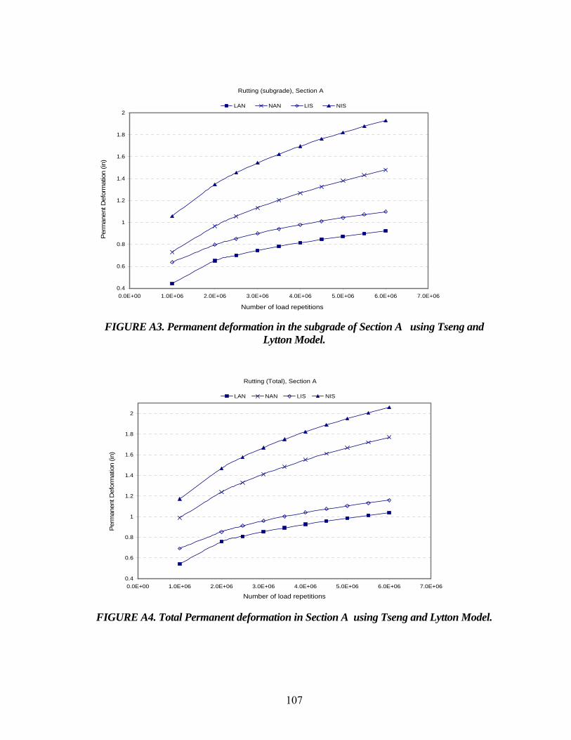
107
Rutting (subgrade), Section A
0.4
0.6
0.8
1
1.2
1.4
1.6
1.8
2
0.0E+00 1.0E+06 2.0E+06 3.0E+06 4.0E+06 5.0E+06 6.0E+06 7.0E+06
Number of load repetitions
Per
man
ent D
efor
mat
ion
(in)
LAN NAN LIS NIS
FIGURE A3. Permanent deformation in the subgrade of Section A using Tseng and
Lytton Model.
Rutting (Total), Section A
0.4
0.6
0.8
1
1.2
1.4
1.6
1.8
2
0.0E+00 1.0E+06 2.0E+06 3.0E+06 4.0E+06 5.0E+06 6.0E+06 7.0E+06
Number of load repetitions
Per
man
ent D
efor
mat
ion
(in)
LAN NAN LIS NIS
FIGURE A4. Total Permanent deformation in Section A using Tseng and Lytton Model.

108
0
3.5
7
10.5
14
17.5
21
-2.0E+02 -1.5E+02 -1.0E+02 -5.0E+01 0.0E+00
Bulk stress (psi), Section A
Dep
th (i
n)
nis nan
FIGURE A5. Bulk stress profiles in the base layer of Section A using non-linear isotropic
and anisotropic properties.
0
3.5
7
10.5
14
17.5
21
0.0E+00 5.0E+00 1.0E+01 1.5E+01 2.0E+01 2.5E+01 3.0E+01 3.5E+01
Deviatoric Stress (psi), Section A
Dep
th(in
)
nis nan
FIGURE A6. Deviatoric stress profiles in the base layer of Section A using non-linear
isotropic and anisotropic properties.

109
0
3.5
7
10.5
14
17.5
21
5.0E-04 1.0E-03 1.5E-03 2.0E-03 2.5E-03 3.0E-03 3.5E-03
Compressive Strain, Section AD
epth
(in)
nis nan
FIGURE A7 Compressive strain profiles in the base layer of Section A using non-linear
isotropic and anisotropic properties.
0
1
2
-6.0E-04 -4.0E-04 -2.0E-04 0.0E+00 2.0E-04 4.0E-04 6.0E-04 8.0E-04 1.0E-03
Compressive Strain, Section A
Dep
th (i
n)
nis nan
FIGURE A8 Compressive strain profiles in the asphalt layer of Section A using non-
linear isotropic and anisotropic properties.

110
0
1
2
0.0E+00 2.0E+01 4.0E+01 6.0E+01 8.0E+01 1.0E+02 1.2E+02 1.4E+02 1.6E+02 1.8E+02
Deviatoric Stress (psi), Section AD
epth
(in)
nis nan
FIGURE A9 Deviatoric stress profiles in the asphalt layer of Section A using non-linear
isotropic and anisotropic properties.
0
3.5
7
10.5
14
17.5
21
-1.5E+02 -1.0E+02 -5.0E+01 0.0E+00 5.0E+01
Bulk stress (psi), Section A
Dep
th
LIS LAN
FIGURE A10 Bulk stress profiles in the base layer of Section A using linear isotropic and
anisotropic properties.

111
0
3.5
7
10.5
14
17.5
21
0.0E+00 5.0E+00 1.0E+01 1.5E+01 2.0E+01 2.5E+01 3.0E+01
Deviatoric Stress (psi), Section AD
epth
LIS LAN
FIGURE A11 Deviatoric stress profiles in the base layer of Section A using linear
isotropic and anisotropic properties.
0
3.5
7
10.5
14
17.5
21
0.0E+00 5.0E-04 1.0E-03 1.5E-03 2.0E-03 2.5E-03 3.0E-03 3.5E-03 4.0E-03
Compressive Strain, Section A
Dep
th
LIS LAN
FIGURE A12 Compressive strain profiles in the base layer of Section A using linear
isotropic and anisotropic properties.

112
0
1
2
-6.0E-04 -4.0E-04 -2.0E-04 0.0E+00 2.0E-04 4.0E-04 6.0E-04 8.0E-04
Compressive Strain, Section AD
epth
(in)
LIS LAN
FIGURE A13 Compressive strain profiles in the asphalt layer of Section A using linear
isotropic and anisotropic properties.
0
1
2
0.0E+00 2.0E+01 4.0E+01 6.0E+01 8.0E+01 1.0E+02 1.2E+02 1.4E+02
Deviatoric Stress (psi), Section A
Dep
th (i
n)
LIS LAN
FIGURE A14 Deviatoric stress profiles in the asphalt layer of Section A using linear
isotropic and anisotropic properties.

113
Tensile Strain VS Depth ,Section A
0
2
4
6
8
10
12
14
16
3.0E-04 4.0E-04 5.0E-04 6.0E-04 7.0E-04 8.0E-04 9.0E-04
Tensile Strain
Dep
th (i
n)
nis nan
FIGURE A15 Tensile strain profiles in the asphalt and base layers of Section A using nonlinear isotropic and anisotropic properties.
Rutting (HMA), Section B
0.02
0.03
0.04
0.05
0.06
0.07
0.08
0.09
0.1
0.0E+00 1.0E+06 2.0E+06 3.0E+06 4.0E+06 5.0E+06 6.0E+06 7.0E+06
Number of load repetitions
Per
man
ent D
efor
mat
ion
(in)
lan nan lis nis
FIGURE A16 HMA permanent deformation in Section B using Tseng and Lytton Model.

114
Rutting (Base), Section B
0.01
0.02
0.03
0.04
0.05
0.06
0.07
0.08
0.09
0.0E+00 1.0E+06 2.0E+06 3.0E+06 4.0E+06 5.0E+06 6.0E+06 7.0E+06
Number of load repetitions
Per
man
ent D
efor
mat
ion
(in)
lan nan lis nis
FIGURE A17 Permanent deformation in the base of Section B using Tseng and Lytton
Model. Rutting (Subgrade), Section B
0.4
0.5
0.6
0.7
0.8
0.9
1
1.1
1.2
1.3
1.4
0.0E+00 1.0E+06 2.0E+06 3.0E+06 4.0E+06 5.0E+06 6.0E+06 7.0E+06
Number of load repetitions
Perm
anen
t Def
orm
atio
n (in
)
lan nan lis nis
FIGURE A18 Permanent deformation in the subgrade of Section B using
Tseng and Lytton Model

115
. Rutting (Total), Section B
0.4
0.6
0.8
1
1.2
1.4
1.6
0.0E+00 1.0E+06 2.0E+06 3.0E+06 4.0E+06 5.0E+06 6.0E+06 7.0E+06
Number of load repetitions
Perm
anen
t Def
orm
atio
n (in
)
lan nan lis nis
FIGURE A19 Total permanent deformation in Section B using Tseng and Lytton Model.
0
4
8
12
16
20
24
28
-8.0E+01 -6.0E+01 -4.0E+01 -2.0E+01 0.0E+00 2.0E+01
Bulk stress (psi), Section B
Dep
th (i
n)
LAN LIS
FIGURE A20 Bulk stress profiles in the base layer of Section B using linear isotropic and
anisotropic properties.

116
0
4
8
12
16
20
24
28
0.0E+00 5.0E+00 1.0E+01 1.5E+01 2.0E+01
Deviatoric Stress (psi) ,Section BD
epth
(in)
LAN LIS
FIGURE A21 Deviatoric stress profiles in the base layer of Section B using linear
isotropic and anisotropic properties.
0
4
8
12
16
20
24
0.0E+00 5.0E-04 1.0E-03 1.5E-03 2.0E-03
Compressive Strain, Section B
Dep
th (i
n)
LAN LIS
Figure A22 Compressive strain profiles in the base layer of Section B using linear
isotropic and anisotropic properties.

117
0
1
2
3
4
-3.0E-04 -2.0E-04 -1.0E-04 0.0E+00 1.0E-04 2.0E-04 3.0E-04 4.0E-04 5.0E-04 6.0E-04
Compressive Strain, Section BD
epth
(in)
LAN LIS
FIGURE A23 Compressive strain profiles in the asphalt layer of Section B using linear
isotropic and anisotropic properties.
0
1
2
3
4
-1.0E+01 1.0E+01 3.0E+01 5.0E+01 7.0E+01 9.0E+01 1.1E+02 1.3E+02
Deviatoric Stress (psi) ,Section B
Dep
th (i
n)
LAN LIS
FIGURE A24 Deviatoric stress profiles in the asphalt layer of Section B using linear
isotropic and anisotropic properties.

118
0
4
8
12
16
20
24
-7.0E+01 -6.0E+01 -5.0E+01 -4.0E+01 -3.0E+01 -2.0E+01 -1.0E+01 0.0E+00
Bulk stress (psi), Section B
Dep
th (i
n)
nis nan
FIGURE A25 Bulk stress profiles in the base layer of Section B using non-linear isotropic
and anisotropic properties.
0
4
8
12
16
20
24
2.0E+00 4.0E+00 6.0E+00 8.0E+00 1.0E+01 1.2E+01 1.4E+01
Deviatoric Stress (psi), Section B
Dep
th (i
n)
nis nan
FIGURE A26 Deviatoric stress profiles in the base layer of Section B using non-linear
isotropic and anisotropic properties.

119
0
4
8
12
16
20
24
5.0E-04 1.0E-03 1.5E-03 2.0E-03 2.5E-03 3.0E-03
Compressive Strain, Section BD
epth
(in)
nis nan
FIGURE A27 Compressive strain profiles in the base layer of Section B using non-linear
isotropic and anisotropic properties.
0
1
2
3
4
-5.0E-04 -3.0E-04 -1.0E-04 1.0E-04 3.0E-04 5.0E-04 7.0E-04 9.0E-04
Compressive Strain, Section B
Dep
th (i
n)
nis nan
FIGURE A28 Compressive strain profiles in the asphalt layer of Section B using non-
linear isotropic and anisotropic properties.

120
0
1
2
3
4
2.0E+00 2.2E+01 4.2E+01 6.2E+01 8.2E+01 1.0E+02 1.2E+02 1.4E+02
Deviatoric Stress (psi), Section BD
epth
(in)
nis nan
FIGURE A29 Deviatoric stress profiles in the asphalt layer of Section B using non-linear
isotropic and anisotropic properties.
Tensile Strain VS Depth ,Section C
3
6
9
12
15
18
1.4E-04 1.6E-04 1.8E-04 2.0E-04 2.2E-04 2.4E-04 2.6E-04 2.8E-04
Tensile Strain
Dep
th (i
n)
lis lan
FIGURE A30 Tensile strain profiles in the asphalt and base layers of Section C using linear isotropic and anisotropic properties.

121
Rutting (HMA), Section D
0.01
0.015
0.02
0.025
0.03
0.035
0.04
0.045
0.05
0.0E+00 1.0E+06 2.0E+06 3.0E+06 4.0E+06 5.0E+06 6.0E+06 7.0E+06
Number of load repetitions
Per
man
ent D
efor
mat
ion
(in)
NAN NIS LIS lan
FIGURE A31 HMA Permanent deformation in Section D using Tseng and Lytton Model.
Rutting (Base), Section D
0
0.05
0.1
0.15
0.2
0.25
0.3
0.35
0.0E+00 1.0E+06 2.0E+06 3.0E+06 4.0E+06 5.0E+06 6.0E+06 7.0E+06
Number of load repetitions
Perm
anen
t Def
orm
atio
n (in
)
NAN NIS LIS lan
FIGURE A32 Permanent deformation in the base of Section D using
Tseng and Lytton Model.
122
Rutting (Subgrade), Section D
0.3
0.5
0.7
0.9
1.1
1.3
1.5
0.0E+00 1.0E+06 2.0E+06 3.0E+06 4.0E+06 5.0E+06 6.0E+06 7.0E+06
Number of load repetitions
Per
man
ent D
efor
mat
ion
(in)
NAN NIS LIS lan
FIGURE A33 Permanent deformation in the sugrade of Section D using
Tseng and Lytton Model.
Rutting (Total), Section D
0.4
0.6
0.8
1
1.2
1.4
1.6
0.00E+00 1.00E+06 2.00E+06 3.00E+06 4.00E+06 5.00E+06 6.00E+06 7.00E+06
Number of load repetitions
Perm
anen
t Def
orm
atio
n (in
)
NAN NIS LIS lan
FIGURE A34 Total permanent deformation in Section D using Tseng and Lytton Model.

123
0
4
8
12
16
20
24
28
-1.5E+02 -1.3E+02 -1.1E+02 -9.0E+01 -7.0E+01 -5.0E+01 -3.0E+01 -1.0E+01 1.0E+01
Bulk stress (psi), Section D
Dep
th (i
n)
LAN LIS
FIGURE A.35 The bulk stress profiles in the base layer of Section D using linear
isotropic and anisotropic properties.
0
4
8
12
16
20
24
28
0.0E+00 5.0E+00 1.0E+01 1.5E+01 2.0E+01 2.5E+01 3.0E+01
Deviatoric stress (psi), Section D
Dep
th (i
n)
LAN LIS
FIGURE A.36 Deviatoric stress profiles in the base layer of Section D using linear
isotropic and anisotropic properties.

124
0
4
8
12
16
20
24
28
0.0E+00 5.0E-04 1.0E-03 1.5E-03 2.0E-03 2.5E-03 3.0E-03 3.5E-03 4.0E-03
Compressive Strain, Section DD
epth
(in)
LAN LIS
FIGURE A.37 Compressive strain profiles in the base layer of Section D using linear
isotropic and anisotropic properties.
0
1
2
-6.0E-04 -4.0E-04 -2.0E-04 0.0E+00 2.0E-04 4.0E-04 6.0E-04 8.0E-04
Compressive Strain, Section D
Dep
th (i
n)
LAN LIS
FIGURE A38 Compressive strain profiles in the asphalt layer of Section D using linear
isotropic and anisotropic properties.

125
0
1
2
0.0E+00 2.0E+01 4.0E+01 6.0E+01 8.0E+01 1.0E+02 1.2E+02 1.4E+02
Deviatoric stress (psi), Section DD
epth
(in)
LAN LIS
FIGURE A39 Deviatoric stress profiles in the asphalt layer of Section D using linear
isotropic and anisotropic properties.
0
4
8
12
16
20
24
28
-2.0E+02 -1.5E+02 -1.0E+02 -5.0E+01 0.0E+00
Bulk stress (psi), Section D
Dep
th (i
n)
NAN NIS
FIGURE A40 Bulk stress profiles in the base layer of Section D using non-linear
isotropic and anisotropic properties

126
0
4
8
12
16
20
24
28
0.0E+00 5.0E+00 1.0E+01 1.5E+01 2.0E+01 2.5E+01 3.0E+01
Deviatoric stress (psi), Section DD
epth
(in)
NAN NIS
FIGURE A41 Deviatoric stress profiles in the base layer of Section D using non-linear
isotropic and anisotropic properties.
0
4
8
12
16
20
24
28
0.0E+00 5.0E-04 1.0E-03 1.5E-03 2.0E-03 2.5E-03 3.0E-03 3.5E-03 4.0E-03
Compressive Strain, Section D
Dep
th (i
n)
NAN NIS
FIGURE A42 Compressive strain profiles in the base layer of Section D using non-linear
isotropic and anisotropic properties.

127
0
1
2
-6.0E-04 -4.0E-04 -2.0E-04 0.0E+00 2.0E-04 4.0E-04 6.0E-04 8.0E-04 1.0E-03
Compressive Strain, Section DD
epth
(in)
NAN NIS
FIGURE A43 Compressive strain profiles in the asphalt layer of Section D using non-
linear isotropic and anisotropic properties.
0
1
2
0.0E+00 2.0E+01 4.0E+01 6.0E+01 8.0E+01 1.0E+02 1.2E+02 1.4E+02 1.6E+02 1.8E+02 2.0E+02
Deviatoric stress (psi), Section D
Dep
th (i
n)
NAN NIS
FIGURE A44 Deviatoric stress profiles in the asphalt layer of Section D using non-linear
isotropic and anisotropic properties.

128
Tensile Strain VS Depth ,Section D
0
2
4
6
8
10
12
14
16
18
20
22
3.0E-04 4.0E-04 5.0E-04 6.0E-04 7.0E-04 8.0E-04 9.0E-04
Tensile Strain
Dep
th (i
n)
NIS NAN
FIGURE A45 Tensile strain profiles in the asphalt and base layers of Section D using
nonlinear isotropic and anisotropic properties. Rutting (HMA), Section E
0.03
0.04
0.05
0.06
0.07
0.08
0.09
0.1
0.0E+00 1.0E+06 2.0E+06 3.0E+06 4.0E+06 5.0E+06 6.0E+06 7.0E+06
Number of load repetitions
Perm
anen
t Def
orm
atio
n (in
)
LIS LAN NIS NAN
FIGURE A46 HMA permanent deformation in Section E using Tseng and Lytton Model.

129
Rutting (Base), Section E
0.02
0.03
0.04
0.05
0.06
0.07
0.08
0.09
0.1
0.11
0.0E+00 1.0E+06 2.0E+06 3.0E+06 4.0E+06 5.0E+06 6.0E+06 7.0E+06
Number of load repetitions
Per
man
ent D
efor
mat
ion
(in)
LIS LAN NIS NAN
FIGURE A47 Permanent deformation in the base of Section E using Tseng and Lytton
Model. Rutting (Subgrade), Section E
0.3
0.4
0.5
0.6
0.7
0.8
0.9
1
1.1
0.0E+00 1.0E+06 2.0E+06 3.0E+06 4.0E+06 5.0E+06 6.0E+06 7.0E+06
Number of load repetitions
Per
man
ent D
efor
mat
ion
(in)
LIS LAN NIS NAN
FIGURE A48 Permanent deformation in the subgrade of Section E using Tseng and
Lytton Model

130
. Rutting (Total), Section E
0.4
0.5
0.6
0.7
0.8
0.9
1
1.1
1.2
0.0E+00 1.0E+06 2.0E+06 3.0E+06 4.0E+06 5.0E+06 6.0E+06 7.0E+06
Number of load repetitions
Per
man
ent D
efor
mat
ion
(in)
LIS LAN NIS NAN
FIGURE A49 Total permanent deformation in Section E using Tseng and Lytton Model.
Rutting (HMA), Section F
0.04
0.05
0.06
0.07
0.08
0.09
0.1
0.11
0.12
0.13
0.14
0.0E+00 1.0E+06 2.0E+06 3.0E+06 4.0E+06 5.0E+06 6.0E+06 7.0E+06
Number of load repetitions
Perm
anen
t Def
orm
atio
n (in
)
LIS LAN NIS NAN
FIGURE A50 HMA permanent deformation in Section F using Tseng and Lytton Model.

131
Rutting (Base), Section F
0.01
0.015
0.02
0.025
0.03
0.035
0.04
0.045
0.0E+00 1.0E+06 2.0E+06 3.0E+06 4.0E+06 5.0E+06 6.0E+06 7.0E+06
Number of load repetitions
Perm
anen
t Def
orm
atio
n (in
)
LIS LAN NIS NAN
FIGURE A51 Permanent deformation in the base of Section F using Tseng and Lytton
Model.
Rutting (Subgrade), Section F
0.2
0.3
0.4
0.5
0.6
0.7
0.8
0.0E+00 1.0E+06 2.0E+06 3.0E+06 4.0E+06 5.0E+06 6.0E+06 7.0E+06
Number of load repetitions
Per
man
ent D
efor
mat
ion
(in)
LIS LAN NIS NAN
FIGURE A52 Permanent deformation in the subgrade of Section F using Tseng and
Lytton Model.

132
Rutting (Total), Section F
0.3
0.4
0.5
0.6
0.7
0.8
0.9
0.0E+00 1.0E+06 2.0E+06 3.0E+06 4.0E+06 5.0E+06 6.0E+06 7.0E+06
Number of load repetitions
Perm
anen
t Def
orm
atio
n (in
)
LIS LAN NIS NAN
FIGURE A53 Total permanent deformation n Section F using Tseng and Lytton Model.
Tensile Strain VS Depth ,Section F
3
6
9
12
15
18
21
24
7.0E-05 9.0E-05 1.1E-04 1.3E-04 1.5E-04 1.7E-04 1.9E-04 2.1E-04 2.3E-04 2.5E-04
Tensile Strain
Dep
th (i
n)
lis lan
FIGURE A54 Tensile strain profiles in the asphalt and base layers of Section D using linear isotropic and anisotropic properties.

133
APPENDIX B
Rutting (HMA ), Section A
0.1
0.2
0.3
0.4
0.5
0.6
0.7
0.0E+00 1.0E+06 2.0E+06 3.0E+06 4.0E+06 5.0E+06 6.0E+06 7.0E+06
Number of load repetitions
Per
man
ent D
efor
mat
ion
(in)
LAN NAN LIS NIS
FIGURE B1 HMA permanent deformation in Section A using AASHTO 2002 Model.
Rutting (Base), Section A
0.05
0.15
0.25
0.35
0.45
0.55
0.0E+00 1.0E+06 2.0E+06 3.0E+06 4.0E+06 5.0E+06 6.0E+06 7.0E+06
Number of load repetitions
Per
man
ent D
efor
mat
ion
(in)
LAN NAN LIS NIS
FIGURE B2 Base permanent deformation in Section A using AASHTO 2002 Model.

134
Rutting (subgrade), Section A
0.1
0.15
0.2
0.25
0.3
0.35
0.4
0.45
0.5
0.0E+00 1.0E+06 2.0E+06 3.0E+06 4.0E+06 5.0E+06 6.0E+06 7.0E+06
Number of load repetitions
Per
man
ent D
efor
mat
ion
(in)
LAN NAN LIS NIS
FIGURE B3 Subgrade permanent deformation in Section A using AASHTO 2002 Model.
Rutting (Total), Section A
0.3
0.5
0.7
0.9
1.1
1.3
1.5
1.7
0.0E+00 1.0E+06 2.0E+06 3.0E+06 4.0E+06 5.0E+06 6.0E+06 7.0E+06
Number of load repetitions
Per
man
ent D
efor
mat
ion
(in)
LAN NAN LIS NIS
FIGURE B4 Total permanent deformation in Section A using AASHTO 2002 Model.

135
Rutting (HMA), Section B
0.15
0.35
0.55
0.75
0.95
1.15
1.35
1.55
0.0E+00 1.0E+06 2.0E+06 3.0E+06 4.0E+06 5.0E+06 6.0E+06 7.0E+06
Number of load repetitions
Per
man
ent D
efor
mat
ion
(in)
lan nan lis nis
FIGURE B5 HMA permanent deformation in Section B using AASHTO 2002 Model.
Rutting (Base), Section B
0.05
0.1
0.15
0.2
0.25
0.3
0.0E+00 1.0E+06 2.0E+06 3.0E+06 4.0E+06 5.0E+06 6.0E+06 7.0E+06
Number of load repetitions
Per
man
ent D
efor
mat
ion
(in)
lan nan lis nis
FIGURE B6 Base permanent deformation in Section B using AASHTO 2002 Model.

136
Rutting (Subgrade), Section B
0.05
0.1
0.15
0.2
0.25
0.3
0.35
0.0E+00 1.0E+06 2.0E+06 3.0E+06 4.0E+06 5.0E+06 6.0E+06 7.0E+06
Number of load repetitions
Per
man
ent D
efor
mat
ion
(in)
lan nan lis nis
FIGURE B7 Subgrade permanent deformation in Section B using AASHTO 2002 Model.
Rutting (Total), Section B
0.3
0.5
0.7
0.9
1.1
1.3
1.5
1.7
1.9
2.1
0.0E+00 1.0E+06 2.0E+06 3.0E+06 4.0E+06 5.0E+06 6.0E+06 7.0E+06
Number of load repetitions
Per
man
ent D
efor
mat
ion
(in)
lan nan lis nis
FIGURE B8 Total permanent deformation in Section B using AASHTO 2002 Model.

137
Rutting (HMA), Section D
0.05
0.15
0.25
0.35
0.45
0.55
0.65
0.75
0.0E+00 1.0E+06 2.0E+06 3.0E+06 4.0E+06 5.0E+06 6.0E+06 7.0E+06
Number of load repetitions
Perm
anen
t Def
orm
atio
n (in
)
NAN NIS LIS lan
FIGURE B9 HMA permanent deformation in Section D using AASHTO 2002 Model.
Rutting (Base), Section D
0.1
0.2
0.3
0.4
0.5
0.6
0.7
0.8
0.0E+00 1.0E+06 2.0E+06 3.0E+06 4.0E+06 5.0E+06 6.0E+06 7.0E+06
Number of load repetitions
Perm
anen
t Def
orm
atio
n (in
)
NAN NIS LIS lan
FIGURE B10 Base permanent deformation in Section D using AASHTO 2002 Model.

138
Rutting (Subgrade), Section D
0
0.05
0.1
0.15
0.2
0.25
0.3
0.35
0.0E+00 1.0E+06 2.0E+06 3.0E+06 4.0E+06 5.0E+06 6.0E+06 7.0E+06
Number of load repetitions
Per
man
ent D
efor
mat
ion
(in)
NAN NIS LIS lan
FIGURE B11 Subgrade permanent deformation in Section D using AASHTO 2002
Model.
Rutting (Total), Section D
0.2
0.4
0.6
0.8
1
1.2
1.4
1.6
1.8
0.0E+00 1.0E+06 2.0E+06 3.0E+06 4.0E+06 5.0E+06 6.0E+06 7.0E+06
Number of load repetitions
Perm
anen
t Def
orm
atio
n (in
)
NAN NIS LIS lan
FIGURE B12 Total permanent deformation in Section D using AASHTO 2002 Model.

139
Rutting (HMA), Section E
0.15
0.35
0.55
0.75
0.95
1.15
1.35
1.55
0.0E+00 1.0E+06 2.0E+06 3.0E+06 4.0E+06 5.0E+06 6.0E+06 7.0E+06
Number of load repetitions
Per
man
ent D
efor
mat
ion
(in)
LIS LAN NIS NAN
FIGURE B13 HMA permanent deformation in Section E using AASHTO 2002 Model.
Rutting (Base), Section E
0.07
0.12
0.17
0.22
0.27
0.32
0.37
0.0E+00 1.0E+06 2.0E+06 3.0E+06 4.0E+06 5.0E+06 6.0E+06 7.0E+06
Number of load repetitions
Per
man
ent D
efor
mat
ion
(in)
LIS LAN NIS NAN
FIGURE B14 Base permanent deformation in Section E using AASHTO 2002 Model.
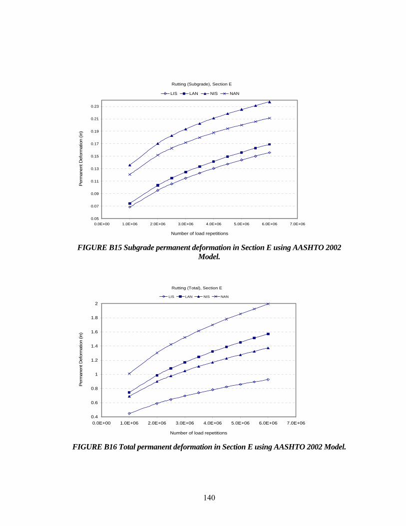
140
Rutting (Subgrade), Section E
0.05
0.07
0.09
0.11
0.13
0.15
0.17
0.19
0.21
0.23
0.0E+00 1.0E+06 2.0E+06 3.0E+06 4.0E+06 5.0E+06 6.0E+06 7.0E+06
Number of load repetitions
Per
man
ent D
efor
mat
ion
(in)
LIS LAN NIS NAN
FIGURE B15 Subgrade permanent deformation in Section E using AASHTO 2002
Model.
Rutting (Total), Section E
0.4
0.6
0.8
1
1.2
1.4
1.6
1.8
2
0.0E+00 1.0E+06 2.0E+06 3.0E+06 4.0E+06 5.0E+06 6.0E+06 7.0E+06
Number of load repetitions
Per
man
ent D
efor
mat
ion
(in)
LIS LAN NIS NAN
FIGURE B16 Total permanent deformation in Section E using AASHTO 2002 Model.

141
Rutting (HMA), Section F
0.2
0.3
0.4
0.5
0.6
0.7
0.8
0.9
1
0.0E+00 1.0E+06 2.0E+06 3.0E+06 4.0E+06 5.0E+06 6.0E+06 7.0E+06
Number of load repetitions
Per
man
ent D
efor
mat
ion
(in)
LIS LAN NIS NAN
FIGURE B17 HMA permanent deformation in Section F using AASHTO 2002 Model.
Rutting (Base), Section F
0.05
0.07
0.09
0.11
0.13
0.15
0.17
0.19
0.21
0.0E+00 1.0E+06 2.0E+06 3.0E+06 4.0E+06 5.0E+06 6.0E+06 7.0E+06
Number of load repetitions
Per
man
ent D
efor
mat
ion
(in)
LIS LAN NIS NAN
FIGURE B18 Base permanent deformation in Section F using AASHTO 2002 Model.

142
Rutting (Subgrade), Section F
0.04
0.06
0.08
0.1
0.12
0.14
0.16
0.18
0.0E+00 1.0E+06 2.0E+06 3.0E+06 4.0E+06 5.0E+06 6.0E+06 7.0E+06
Number of load repetitions
Per
man
ent D
efor
mat
ion
(in)
LIS LAN NIS NAN
FIGURE B19 Subgrade permanent deformation in Section F using
AASHTO 2002 Model.
Rutting (Total), Section F
0.2
0.4
0.6
0.8
1
1.2
1.4
0.0E+00 1.0E+06 2.0E+06 3.0E+06 4.0E+06 5.0E+06 6.0E+06 7.0E+06
Number of load repetitions
Per
man
ent D
efor
mat
ion
(in)
LIS LAN NIS NAN
FIGURE B20 Total permanent deformation in Section F using AASHTO 2002 Model.

143
APPENDIX C
TABLE C1 THE ANALYSIS RESULTS OF ASPHALT PAVEMENT WITH BINDER GRADE OF PG58-28, BASE LAYER WITH MODULUS OF 42.0 KSI IN HOUSTON UNDER AADT OF 3000
Thickness (in) Material Rutting (in) Longitudinal Cracking(ft/mi)
Alligator Cracking (%)
HMA Base Subgrade HMA Base Subgrade Total Surface Depth=0.5 Bottom-up cracking
IRI(in/mi)
4 10 A-2-5 (28 ksi) 0.4896 0.0541 0.3126 0.8563 1170 514 87 195.5
8 10 A-2-5 0.3812 0.0287 0.2411 0.651 8420 7410 19.4 86.4
4 12 A-2-5 0.4112 0.0526 0.3113 0.7751 1160 519 86.7 189.2
8 12 A-2-5 0.3138 0.0309 0.3815 0.7262 8280 7230 18.1 82.5
4 15 A-2-5 0.4875 0.0679 0.2622 0.8176 1030 430 86.7 192.6
8 15 A-2-5 0.3829 0.0369 0.3639 0.7837 8290 7210 19.3 86.3
4 10 A-6 (18 ksi) 0.406 0.052 0.3334 0.7914 1500 713 90.8 247.9
8 10 A-6 0.366 0.0283 0.2551 0.6494 8200 7070 26.2 102.1
4 12 A-6 0.4065 0.0575 0.3115 0.7755 1250 568 90 236.3
8 12 A-6 0.3021 0.0304 0.2408 0.5733 7870 6630 23.7 97.4
4 15 A-6 0.4057 0.0653 0.2762 0.7472 1030 443 89.2 226.6
8 15 A-6 0.3735 0.0365 0.2247 0.6347 7750 6440 23.5 100.9
4 10 A-7-6 (8 ksi) 0.4749 0.0556 0.3692 0.8997 1300 588 93 307.3
8 10 A-7-6 0.3531 0.03 0.2714 0.6545 6080 4300 33.3 116.1
4 12 A-7-6 0.4758 0.0608 0.3406 0.8772 903 376 91.9 281.2
8 12 A-7-6 0.3593 0.0335 0.2556 0.6484 5480 3610 30.3 114.6
4 15 A-7-6 0.4766 0.0685 0.2962 0.8413 615 231 90.6 259.2
8 15 A-7-6 0.3672 0.0384 0.2338 0.6394 5000 3060 27.1 113.1

144
TABLE C2 THE ANALYSIS RESULTS OF ASPHALT PAVEMENT WITH BINDER GRADE OF PG58-28, BASE LAYER WITH MODULUS OF 38.0 KSI IN HOUSTON UNDER AADT OF 3000
Thickness (in) Material Rutting (in) Longitudinal
Cracking(ft/mi) Alligator
Cracking (%)
HMA Base Subgrade HMA Base Subgrade Total Surface Depth=0.5 Bottom-up cracking
IRI(in/mi)
4 10 A-2-5 (28 ksi) 0.4137 0.0524 0.3131 0.7792 1280 576 88.5 205.9
8 10 A-2-5 0.3107 0.0271 0.2406 0.5784 8550 7590 20.3 83.4
4 12 A-2-5 0.4143 0.0583 0.4149 0.8875 1230 545 88.5 205.2
8 12 A-2-5 0.3114 0.0304 0.3842 0.726 8500 7530 20.2 83.3
4 15 A-2-5 0.4122 0.0661 0.2629 0.7412 1170 508 88.3 204.2
8 15 A-2-5 0.4468 0.0378 0.3663 0.8509 8580 7600 23 87.1
4 10 A-6 (18 ksi) 0.4106 0.0515 0.3372 0.7993 1700 816 92.4 276.7
8 10 A-6 0.2971 0.0265 0.2553 0.5789 8330 7260 27.5 99.1
4 12 A-6 0.4108 0.0571 0.3155 0.7834 1450 671 91.8 264.4
8 12 A-6 0.2997 0.0298 0.2429 0.5724 8160 7020 26.2 98.6
4 15 A-6 0.4092 0.065 0.2799 0.7541 1220 535 91.1 252
8 15 A-6 0.3028 0.0345 0.2258 0.5631 7990 6770 24.8 97.9
4 10 A-7-6 (8 ksi) 0.4816 0.0549 0.3743 0.9108 1530 707 94.4 347.7
8 10 A-7-6 0.3505 0.0293 0.274 0.6538 6600 4900 36.5 117.9
4 12 A-7-6 0.4818 0.0602 0.346 0.888 1110 473 93.5 318.4
8 12 A-7-6 0.3563 0.0327 0.2586 0.6476 6100 4290 33.6 116.3
4 15 A-7-6 0.4814 0.068 0.3014 0.8508 778 302 92.4 291.3
8 15 A-7-6 0.3639 0.0376 0.2371 0.6386 5680 3760 30.3 114.6

145
TABLE C3 THE ANALYSIS RESULTS OF ASPHALT PAVEMENT WITH BINDER GRADE OF PG58-28, BASE LAYER WITH MODULUS OF 35.0 KSI IN HOUSTON UNDER AADT OF 3000
Thickness (in) Material Rutting (in) Longitudinal
Cracking(ft/mi) Alligator
Cracking (%)
HMA Base Subgrade HMA Base Subgrade Total Surface Depth=0.5 Bottom-up cracking
IRI(in/mi)
4 10 A-2-5 (28 ksi) 0.4962 0.0538 0.3164 0.8664 1470 662 91.1 243.1
TABLE C3 CONTINUED
8 10 A-2-5 0.3759 0.0279 0.2428 0.6466 8830 7970 24.3 88.3
4 12 A-2-5 0.4182 0.0583 0.4174 0.8939 1440 651 90.7 234
8 12 A-2-5 0.3088 0.0301 0.3834 0.7223 8750 7870 22.8 84.3
4 15 A-2-5 0.493 0.0682 0.2651 0.8263 1410 621 91.1 243.6
8 15 A-2-5 0.3766 0.0362 0.3631 0.7759 8800 7920 24.4 88.3
4 10 A-6 (18 ksi) 0.4145 0.0513 0.34 0.8058 1890 912 93.5 304.3
8 10 A-6 0.3611 0.0273 0.2586 0.647 8640 7680 31.3 104.5
4 12 A-6 0.4146 0.057 0.3185 0.7901 1650 769 93 291.7
8 12 A-6 0.2976 0.0294 0.2447 0.5717 8390 7320 28.5 99.6
4 15 A-6 0.4128 0.0651 0.2832 0.7611 1420 636 92.5 279.6
8 15 A-6 0.3673 0.0356 0.2291 0.632 8360 7260 28.9 103.3
4 10 A-7-6 (8 ksi) 0.4872 0.0545 0.3786 0.9203 1750 822 95.3 388.8
8 10 A-7-6 0.348 0.0286 0.2762 0.6528 7010 5400 39.3 119.6
4 12 A-7-6 0.487 0.0599 0.3507 0.8976 1310 573 94.6 355
8 12 A-7-6 0.3535 0.0321 0.2611 0.6467 6610 4870 36.5 117.9
4 15 A-7-6 0.4859 0.0679 0.3063 0.8601 959 383 93.7 326.4
8 15 A-7-6 0.3606 0.0371 0.24 0.6377 6260 4410 33.4 116.2

146
TABLE C4 THE ANALYSIS RESULTS OF ASPHALT PAVEMENT WITH BINDER GRADE OF PG58-28, BASE LAYER WITH MODULUS OF 31.5 KSI IN HOUSTON UNDER AADT OF 3000
Thickness (in) Material Rutting (in) Longitudinal
Cracking(ft/mi) Alligator
Cracking (%)
HMA Base Subgrade HMA Base Subgrade Total Surface Depth=0.5 Bottom-up cracking
IRI(in/mi)
4 10 A-2-5 (28 ksi) 0.4213 0.0519 0.3181 0.7913 1660 764 92.3 261.6
8 10 A-2-5 0.3061 0.0261 0.2424 0.5746 8930 8130 25.1 85.3
4 12 A-2-5 0.4216 0.0581 0.4216 0.9013 1650 758 92.3 263
8 12 A-2-5 0.3061 0.0295 0.3866 0.7222 8930 8120 25.1 85.3
TABLE C4 CONTINUED
4 15 A-2-5 0.4194 0.0662 0.2674 0.753 1640 749 92.4 264.2
8 15 A-2-5 0.4382 0.037 0.3692 0.8444 9070 8300 29.5 90
4 10 A-6 (18 ksi) 0.4195 0.0507 0.3437 0.8139 2120 1040 94.6 343.3
8 10 A-6 0.2931 0.0254 0.2586 0.5771 8710 7790 32.2 101.4
4 12 A-6 0.4195 0.0566 0.3224 0.7985 1900 901 94.3 329.2
8 12 A-6 0.2951 0.0288 0.2468 0.5707 8620 7640 31.2 100.9
4 15 A-6 0.4173 0.0647 0.2873 0.7693 1680 770 93.9 316.2
8 15 A-6 0.2974 0.0334 0.2303 0.5611 8520 7500 29.9 100.3
4 10 A-7-6 (8 ksi) 0.4949 0.0537 0.3838 0.9324 2040 1000 96.2 444.5
8 10 A-7-6 0.3453 0.0278 0.2789 0.652 7450 5950 42.6 121.8
4 12 A-7-6 0.4941 0.0592 0.3562 0.9095 1580 709 95.6 408.2
8 12 A-7-6 0.3504 0.0312 0.2641 0.6457 7120 5500 40 120
4 15 A-7-6 0.4921 0.0673 0.3119 0.8713 1200 495 95 374.3
8 15 A-7-6 0.357 0.0362 0.2434 0.6366 6840 5110 36.9 118.1

147
TABLE C5 THE ANALYSIS RESULTS OF ASPHALT PAVEMENT WITH BINDER GRADE OF PG58-28, BASE LAYER WITH MODULUS OF 28.0 KSI IN HOUSTON UNDER AADT OF 3000
TABLE C5 CONTINUED
Thickness (in) Material Rutting (in) Longitudinal
Cracking(ft/mi) Alligator
Cracking (%)
HMA Base Subgrade HMA Base Subgrade Total Surface Depth=0.5 Bottom-up cracking
IRI(in/mi)
4 10 A-2-5 (28 ksi) 0.4254 0.0515 0.3214 0.7983 1890 882 93.7 296.9
8 10 A-2-5 0.3034 0.0256 0.2439 0.5729 9090 8360 27.7 86.5
4 12 A-2-5 0.4257 0.0577 0.4261 0.9095 1910 894 93.8 300.3
8 12 A-2-5 0.3032 0.029 0.39 0.7222 9100 8370 27.9 86.5
4 15 A-2-5 0.4234 0.0659 0.2708 0.7601 1930 904 93.9 303.4
8 15 A-2-5 0.4334 0.0364 0.3733 0.8431 9260 8580 33 91.8
4 10 A-6 (18 ksi) 0.4254 0.0501 0.3477 0.8232 2400 1190 95.6 389.2
8 10 A-6 0.3554 0.026 0.2626 0.644 9020 8230 37.4 107.8
4 12 A-6 0.4252 0.0561 0.3267 0.808 2200 1070 95.3 377.1
8 12 A-6 0.2923 0.0281 0.2491 0.5695 8830 7950 34.2 102.5
4 15 A-6 0.4227 0.0642 0.2918 0.7787 1990 941 95.1 362.6
8 15 A-6 0.36 0.0342 0.2344 0.6286 8870 8000 35.4 106.7
4 10 A-7-6 (8 ksi) 0.5039 0.0528 0.3894 0.9461 2380 1160 96.9 517
8 10 A-7-6 0.3422 0.0269 0.2817 0.6508 7850 6500 46.1 124.4
4 12 A-7-6 0.5024 0.0584 0.3622 0.923 1920 883 96.5 473.5
8 12 A-7-6 0.3469 0.0303 0.2674 0.6446 7600 6130 43.7 122.6
4 15 A-7-6 0.4995 0.0666 0.3182 0.8843 1510 647 96 434.8
8 15 A-7-6 0.3531 0.0352 0.2472 0.6355 7390 5820 40.8 120.6

148
TABLE C6 THE ANALYSIS RESULTS OF ASPHALT PAVEMENT WITH BINDER GRADE OF PG76-22, BASE LAYER WITH MODULUS OF 42.0 KSI IN HOUSTON UNDER AADT OF 3000
Thickness (in) Material Rutting (in) Longitudinal
Cracking(ft/mi) Alligator
Cracking (%)
HMA Base Subgrade HMA Base Subgrade Total Surface Depth=0.5 Bottom-up cracking
IRI(in/mi)
4 10 A-2-5 (28ksi) 0.2758 0.0479 0.3072 0.6309 1850 916 92.9 275.9 8 10 A-2-5 0.1988 0.0234 0.2323 0.4545 8770 7930 25.6 85.5 4 15 A-2-5 0.2752 0.061 0.2588 0.595 1630 779 92.6 268.8 8 15 A-2-5 0.1999 0.0307 0.3559 0.5865 8690 7810 25.2 85.4 4 10 A-6 (18ksi) 0.2733 0.0473 0.3294 0.65 2350 1210 95.3 372.3 8 10 A-6 0.1858 0.023 0.2462 0.455 8290 7250 33.8 102.3 4 15 A-6 0.2724 0.0601 0.2736 0.6061 1690 804 94.3 333.6 8 15 A-6 0.1907 0.0303 0.2186 0.4396 8050 6890 30.6 100.6 4 10 A-7-6 (8ksi) 0.3142 0.0507 0.3648 0.7297 2030 1000 96.6 485.6 8 10 A-7-6 0.2113 0.0257 0.2635 0.5005 5960 4230 45.5 124 4 12 A-7-6 0.3128 0.0558 0.337 0.7056 1510 686 96 434.8 8 12 A-7-6 0.216 0.0289 0.249 0.4939 5590 3790 42.2 121.5 4 15 A-7-6 0.3104 0.0632 0.2933 0.6669 1090 452 95.3 391.3
TABLE C7 THE ANALYSIS RESULTS OF ASPHALT PAVEMENT WITH BINDER GRADE OF PG76-22, BASE LAYER WITH MODULUS OF 38.0 KSI IN HOUSTON UNDER AADT OF 3000
Thickness (in) Material Rutting (in) Longitudinal
Cracking(ft/mi) Alligator
Cracking (%)
HMA Base Subgrade HMA Base Subgrade Total Surface Depth=0.5 Bottom-up cracking
IRI(in/mi)
4 10 A-7-6 (8ksi) 0.3199 0.0499 0.3697 0.7395 2350 1180 97.2 550.9
8 10 A-7-6 0.2095 0.0249 0.2658 0.5002 6410 4730 48.3 126.2
4 12 A-7-6 0.318 0.055 0.3422 0.7152 1810 847 96.7 495.3
8 12 A-7-6 0.2138 0.0281 0.2517 0.4936 6110 4360 45.2 123.7
4 15 A-7-6 0.3148 0.0625 0.2985 0.6758 1340 579 96.1 442.1
8 15 A-7-6 0.2195 0.0326 0.2318 0.4839 5940 4120 41.5 121

149
TABLE C8 THE ANALYSIS RESULTS OF ASPHALT PAVEMENT WITH BINDER GRADE OF PG76-22, BASE LAYER WITH MODULUS OF 35.0 KSI IN HOUSTON UNDER AADT OF 3000
Thickness (in) Material Rutting (in) Longitudinal
Cracking(ft/mi) Alligator Cracking
(%)
HMA Base Subgrade HMA Base Subgrade Total Surface Depth=0.5 Bottom-up cracking
IRI(in/mi)
4 10 A-2-5 (28ksi) 0.2812 0.0474 0.3104 0.639 2300 1160 94.9 342.6
8 10 A-2-5 0.1958 0.0226 0.2335 0.4519 9060 8340 29.7 87.4
4 15 A-2-5 0.2808 0.0609 0.2614 0.6031 2200 1100 94.9 342.6
8 15 A-2-5 0.1963 0.0298 0.3547 0.5808 9040 8310 29.6 87.4
4 10 A-6 (18ksi) 0.2802 0.0464 0.3355 0.6621 2860 1520 96.5 459.4
8 10 A-6 0.183 0.022 0.2491 0.4541 8630 7710 38 104.7
4 15 A-6 0.2785 0.0596 0.2805 0.6186 2250 1120 96 415.8
8 15 A-6 0.187 0.0293 0.2227 0.439 8480 7480 35.3 103.1
4 10 A-7-6 (8ksi) 0.3249 0.0493 0.3739 0.7481 2640 1350 97.6 618.7
8 10 A-7-6 0.2078 0.0243 0.2678 0.4999 6760 5160 50.6 128.3
4 12 A-7-6 0.3225 0.0546 0.3468 0.7239 2100 1000 97.3 555.8
8 12 A-7-6 0.2118 0.0275 0.254 0.4933 6520 4840 47.7 125.7
TABLE C9 THE ANALYSIS RESULTS OF ASPHALT PAVEMENT WITH BINDER GRADE OF PG76-22, BASE LAYER WITH MODULUS OF 31.5 KSI IN HOUSTON UNDER AADT OF 3000
Thickness (in) Material Rutting (in) Longitudinal
Cracking(ft/mi) Alligator Cracking
(%)
HMA Base Subgrade HMA Base Subgrade Total Surface Depth=0.5 Bottom-up cracking
IRI(in/mi)
4 10 A-7-6 (8ksi) 0.3312 0.0484 0.3788 0.7584 3000 1580 98 703.3
8 10 A-7-6 0.2059 0.0235 0.2701 0.4995 7140 5630 53.3 703.3
4 12 A-7-6 0.3285 0.0537 0.3521 0.7343 2460 1220 97.7 703.3
8 12 A-7-6 0.2096 0.0266 0.2568 0.493 6950 5360 50.6 128.3
4 15 A-7-6 0.3246 0.0615 0.3088 0.6949 1970 908 97.4 572.7
8 15 A-7-6 0.2145 0.0312 0.2377 0.4834 6860 5220 47.5 125.5

150
TABLE C10 THE ANALYSIS RESULTS OF ASPHALT PAVEMENT WITH BINDER GRADE OF PG76-22, BASE LAYER WITH MODULUS OF 28.0 KSI IN HOUSTON UNDER AADT OF 3000
Thickness (in) Material Rutting (in) Longitudinal
Cracking(ft/mi) Alligator Cracking
(%)
HMA Base Subgrade HMA Base Subgrade Total Surface Depth=0.5 Bottom-up cracking
IRI(in/mi)
4 10 A-7-6 (8ksi) 0.3384 0.0474 0.3841 0.7699 3420 1850 98.4 812.2
8 10 A-7-6 0.2039 0.0226 0.2726 0.4991 7500 6090 56 133.8
4 12 A-7-6 0.3353 0.0528 0.3579 0.746 2890 1480 98.2 737.2
8 12 A-7-6 0.2073 0.0257 0.2596 0.4926 7360 5880 53.7 131.2
4 15 A-7-6 0.331 0.0606 0.3149 0.7065 2390 1150 97.9 667
8 15 A-7-6 0.2118 0.0302 0.2411 0.4831 7300 5780 50.8 128.3
4 10 A-2-5 0.2876 0.0466 0.3161 0.6503 2860 1500 96.4 434.6
8 10 A-2-5 0.1923 0.0216 0.2361 0.45 9290 8660 34.1 89.7
4 15 A-2-5 0.2873 0.0601 0.2676 0.615 2910 1530 96.5 444.2
8 15 A-2-5 0.1919 0.0287 0.3618 0.5824 9300 8690 34.7 90
4 10 A-6 (18ksi) 0.289 0.0451 0.3427 0.6768 3510 1940 97.5 585.2
8 10 A-6 0.1799 0.0208 0.2525 0.4532 8930 8130 42.7 107.7
4 15 A-6 0.2865 0.0585 0.2887 0.6337 3020 1590 97.2 539.2

151
TABLE C11 THE ANALYSIS RESULTS OF ASPHALT PAVEMENT WITH BINDER GRADE OF PG76-22 IN NEW YORK CITY UNDER AADT OF 3000
Thickness (in) Material Rutting (in) Longitudinal
Cracking(ft/mi) Alligator
Cracking (%)
HMA Base Base Subgrade HMA Base Subgrade Total Surface Depth=0.5 Bottom-up cracking IRI(in/mi)
4 10 A-1-a (42ksi) A-7-6 0.135 0.0506 0.3116 0.4972 568 249 82.5 210.8
4 10 A-1-a A-7-6 0.135 0.0506 0.3116 0.4972 568 249 82.5 210.8
8 10 A-1-a A-7-6 0.097 0.0266 0.2276 0.3512 1340 589 17.3 129.7
4 15 A-1-a A-7-6 0.1353 0.0622 0.2508 0.4483 231 86 75 183.7
4 15 A-1-a A-6 0.1396 0.059 0.2405 0.4391 544 240 73.1 165.4
4 15 A-1-a A-7-6 0.1353 0.0622 0.2508 0.4483 231 86 75 183.7
4 10 A-1-b (38ksi) A-7-6 0.1396 0.0493 0.3243 0.5132 771 347 86.8 237.9
8 10 A-1-b A-7-6 0.0963 0.0251 0.2337 0.3551 2000 1000 21.1 131.1
4 10 A-2-4 (35.0ksi) A-7-6 0.1548 0.0462 0.3439 0.5449 1430 683 92.9 323.3
4 10 A-2-4 A-7-6 0.1548 0.0462 0.3439 0.5449 1430 683 92.9 323.3
8 10 A-2-4 A-7-6 0.0945 0.0221 0.2409 0.3575 3210 1870 27.4 133.8
4 15 A-2-4 A-7-6 0.1523 0.0566 0.2782 0.4871 850 366 90.2 273.5
4 15 A-2-4 A-6 0.1522 0.0545 0.2612 0.4679 1410 684 88.5 240.2
4 15 A-2-4 A-7-6 0.1523 0.0566 0.2782 0.4871 850 366 90.2 273.5
4 10 A-2-4(31.5 ksi) A-7-6 0.1582 0.0452 0.3485 0.5519 1670 816 94 355.7
8 10 A-2-4 A-7-6 0.0935 0.0213 0.2429 0.3577 3630 2220 29.5 134.8
4 10 A-2-5 (28ksi) A-7-6 0.1621 0.044 0.3535 0.5596 1960 1000 95 397.3
4 10 A-2-5 A-7-6 0.1621 0.044 0.3535 0.5596 1960 1000 95 397.3
8 10 A-2-5 A-7-6 0.0924 0.0204 0.2451 0.3579 4080 2610 31.8 135.9
4 15 A-2-5 A-7-6 0.1585 0.0548 0.2894 0.5027 1300 588 93.3 334.9
4 15 A-2-5 A-6 0.1567 0.0531 0.2693 0.4791 1930 1000 92 289
4 15 A-2-5 A-7-6 0.1585 0.0548 0.2894 0.5027 1300 588 93.3 334.9
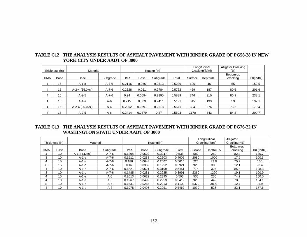
152
TABLE C12 THE ANALYSIS RESULTS OF ASPHALT PAVEMENT WITH BINDER GRADE OF PG58-28 IN NEW YORK CITY UNDER AADT OF 3000
Thickness (in) Material Rutting (in) Longitudinal
Cracking(ft/mi) Alligator Cracking
(%)
HMA Base Base Subgrade HMA Base Subgrade Total Surface Depth=0.5 Bottom-up cracking IRI(in/mi)
4 15 A-1-a A-7-6 0.2116 0.066 0.2513 0.5289 126 46 55 152.5
4 15 A-2-4 (35.0ksi) A-7-6 0.2328 0.061 0.2784 0.5722 469 187 80.5 201.6
4 15 A-2-5 A-7-6 0.24 0.0594 0.2895 0.5889 746 310 86.9 238.1
4 15 A-1-a A-6 0.215 0.063 0.2411 0.5191 315 133 53 137.1
4 15 A-2-4 (35.0ksi) A-6 0.2362 0.0591 0.2618 0.5571 834 376 78.2 179.4
4 15 A-2-5 A-6 0.2414 0.0579 0.27 0.5693 1170 543 84.8 209.7
TABLE C13 THE ANALYSIS RESULTS OF ASPHALT PAVEMENT WITH BINDER GRADE OF PG76-22 IN WASHINGTON STATE UNDER AADT OF 3000
Thickness (in) Material Rutting(in) Longitudinal
Cracking(ft/mi) Alligator Cracking (%)
HMA Base Base Subgrade HMA Base Subgrade Total Surface Depth=0.5 Bottom-up cracking IRI (in/mi)
4 10 A-1-a (42ksi) A-7-6 0.1804 0.0529 0.3047 0.538 582 259 82.4 180.7 8 10 A-1-a A-7-6 0.1511 0.0288 0.2203 0.4002 2080 1000 17.5 100.3 4 15 A-1-a A-7-6 0.186 0.0648 0.2507 0.5015 225 83.8 75.2 155 8 15 A-1-a A-7-6 0.16 0.0369 0.1952 0.3921 926 305 12.1 98.4 4 10 A-1-b A-7-6 0.1821 0.0521 0.3109 0.5451 714 324 85.4 198.3 8 10 A-1-b A-7-6 0.1485 0.0281 0.2225 0.3991 2360 1220 19.1 100.9 4 15 A-1-a A-6 0.2013 0.0622 0.2395 0.503 536 236 74.2 150.5 4 10 A-1-a A-6 0.1967 0.0499 0.2953 0.5419 928 449 78.8 164.1 8 10 A-1-a A-6 0.1631 0.0265 0.2213 0.4109 5320 3890 12.4 96.9 4 10 A-1-b A-6 0.1978 0.0493 0.2991 0.5462 1070 523 82.1 177.6

153
TABLE C13 CONTINUED
4 10 A-2-4 (35.0ksi) A-7-6 0.2021 0.0497 0.3447 0.5965 1390 674 93.1 299.9 8 10 A-2-4 A-7-6 0.1476 0.0248 0.2412 0.4136 4260 2750 29.3 105.3 4 15 A-2-4 A-7-6 0.2028 0.0605 0.2784 0.5417 811 349 90.5 252
4 15 A-2-4 A-6 0.2123 0.0587 0.2616 0.5326 1370 659 89.3 231.8 4 10 A-2-4 A-6 0.2106 0.0473 0.3139 0.5718 1860 957 91 255.5
4 10 A-2-4(31.5 ksi) A-7-6 0.2053 0.0488 0.3494 0.6035 1630 805 94.3 335.7 8 10 A-2-4 A-7-6 0.1458 0.0239 0.2433 0.413 4810 3270 31.9 106.5
4 10 A-2-5 (28ksi) A-7-6 0.2091 0.0477 0.3544 0.6112 1920 1000 95.3 382.4 8 10 A-2-5 A-7-6 0.1438 0.0229 0.2456 0.4123 5380 3840 34.7 108 4 15 A-2-5 A-7-6 0.2077 0.0588 0.2895 0.556 1230 558 93.7 316.1
4 15 A-2-5 A-6 0.2155 0.0575 0.2697 0.5427 1860 933 92.8 289.1 4 10 A-2-5 A-6 0.2149 0.0459 0.321 0.5818 2330 1230 93.7 315.5
8 10 A-2-5 A-6 0.1557 0.0216 0.2344 0.4117 7890 6830 26 102.1
TABLE C14 THE ANALYSIS RESULTS OF ASPHALT PAVEMENT WITH BINDER GRADE OF PG58-28 IN WASHINGTON STATE UNDER AADT OF 3000
Thickness (in) Material Rutting(in) Longitudinal
Cracking(ft/mi) Alligator Cracking(%)
HMA Base Base Subgrade HMA Base Subgrade Total Surface Depth=0.5 Bottom-up cracking IRI(in/mi)
4 15 A-2-5 A-7-6 0.342 0.0642 0.2898 0.696 691 285 87 209.2
4 15 A-1-a A-7-6 0.3154 0.069 0.2515 0.6359 122 43.8 53.6 121.9
4 15 A-2-4 A-7-6 0.3382 0.0656 0.2787 0.6825 437 174 80.1 170.5
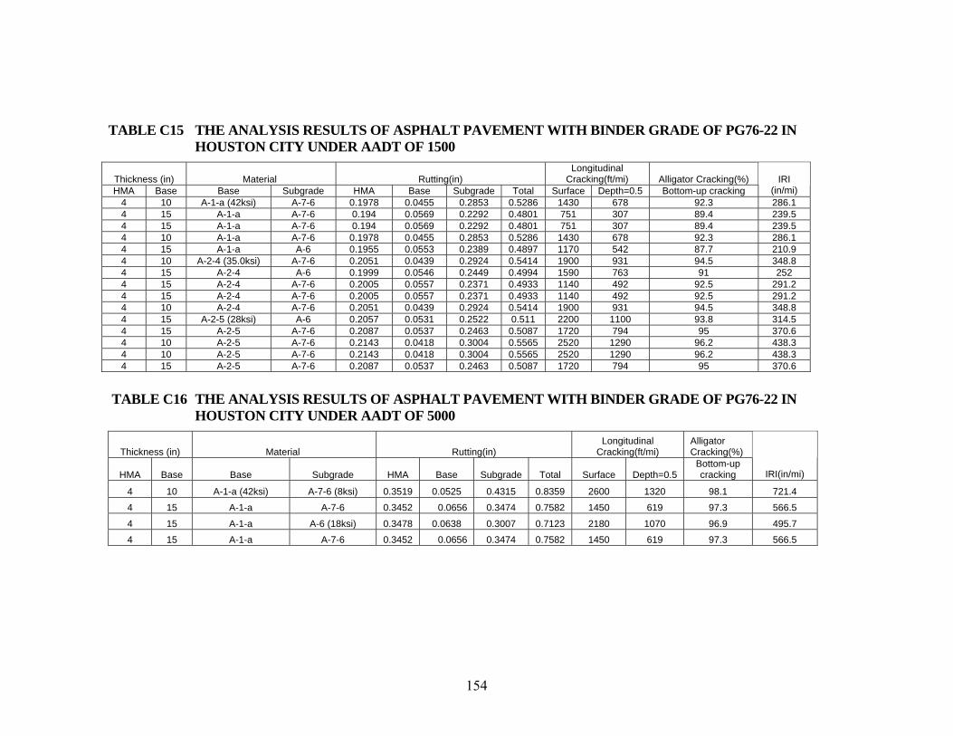
154
TABLE C15 THE ANALYSIS RESULTS OF ASPHALT PAVEMENT WITH BINDER GRADE OF PG76-22 IN HOUSTON CITY UNDER AADT OF 1500
Thickness (in) Material Rutting(in) Longitudinal
Cracking(ft/mi) Alligator Cracking(%) HMA Base Base Subgrade HMA Base Subgrade Total Surface Depth=0.5 Bottom-up cracking
IRI (in/mi)
4 10 A-1-a (42ksi) A-7-6 0.1978 0.0455 0.2853 0.5286 1430 678 92.3 286.1 4 15 A-1-a A-7-6 0.194 0.0569 0.2292 0.4801 751 307 89.4 239.5 4 15 A-1-a A-7-6 0.194 0.0569 0.2292 0.4801 751 307 89.4 239.5 4 10 A-1-a A-7-6 0.1978 0.0455 0.2853 0.5286 1430 678 92.3 286.1 4 15 A-1-a A-6 0.1955 0.0553 0.2389 0.4897 1170 542 87.7 210.9 4 10 A-2-4 (35.0ksi) A-7-6 0.2051 0.0439 0.2924 0.5414 1900 931 94.5 348.8 4 15 A-2-4 A-6 0.1999 0.0546 0.2449 0.4994 1590 763 91 252 4 15 A-2-4 A-7-6 0.2005 0.0557 0.2371 0.4933 1140 492 92.5 291.2 4 15 A-2-4 A-7-6 0.2005 0.0557 0.2371 0.4933 1140 492 92.5 291.2 4 10 A-2-4 A-7-6 0.2051 0.0439 0.2924 0.5414 1900 931 94.5 348.8 4 15 A-2-5 (28ksi) A-6 0.2057 0.0531 0.2522 0.511 2200 1100 93.8 314.5 4 15 A-2-5 A-7-6 0.2087 0.0537 0.2463 0.5087 1720 794 95 370.6 4 10 A-2-5 A-7-6 0.2143 0.0418 0.3004 0.5565 2520 1290 96.2 438.3 4 10 A-2-5 A-7-6 0.2143 0.0418 0.3004 0.5565 2520 1290 96.2 438.3 4 15 A-2-5 A-7-6 0.2087 0.0537 0.2463 0.5087 1720 794 95 370.6
TABLE C16 THE ANALYSIS RESULTS OF ASPHALT PAVEMENT WITH BINDER GRADE OF PG76-22 IN HOUSTON CITY UNDER AADT OF 5000
Thickness (in) Material Rutting(in) Longitudinal
Cracking(ft/mi) Alligator Cracking(%)
HMA Base Base Subgrade HMA Base Subgrade Total Surface Depth=0.5 Bottom-up cracking IRI(in/mi)
4 10 A-1-a (42ksi) A-7-6 (8ksi) 0.3519 0.0525 0.4315 0.8359 2600 1320 98.1 721.4
4 15 A-1-a A-7-6 0.3452 0.0656 0.3474 0.7582 1450 619 97.3 566.5
4 15 A-1-a A-6 (18ksi) 0.3478 0.0638 0.3007 0.7123 2180 1070 96.9 495.7 4 15 A-1-a A-7-6 0.3452 0.0656 0.3474 0.7582 1450 619 97.3 566.5

155
TABLE C16 CONTINUED
8 10 A-1-a A-7-6 0.2249 0.0262 0.3116 0.5627 6300 4530 57.7 132
4 10 A-1-a A-7-6 0.3519 0.0525 0.4315 0.8359 2600 1320 98.1 721.4 4 10 A-1-b (38ksi) A-7-6 0.3589 0.0517 0.4373 0.8479 2970 1550 98.5 827.8 4 10 A-2-4 (35.0ksi) A-7-6 0.3649 0.0511 0.4422 0.8582 3310 1770 98.7 929.4 8 10 A-2-4 A-7-6 0.2212 0.0249 0.3166 0.5627 7050 5440 62.4 138.6 4 15 A-2-4 A-7-6 0.3567 0.0648 0.3592 0.7807 2120 1000 98.2 738.3
4 15 A-2-4 A-6 0.3556 0.0635 0.3082 0.7273 2850 1470 97.8 631.1
4 15 A-2-4 A-7-6 0.3567 0.0648 0.3592 0.7807 2120 1000 98.2 738.3 4 10 A-2-4 A-7-6 0.3649 0.0511 0.4422 0.8582 3310 1770 98.7 929.4 4 10 A-2-4(31.5 ksi) A-7-6 0.3726 0.0503 0.4479 0.8708 3720 2040 98.9 1064.9 4 10 A-2-5 (28ksi) A-7-6 0.3812 0.0493 0.4541 0.8846 4170 2370 100 1231.8 8 10 A-2-5 A-7-6 0.2171 0.0232 0.3222 0.5625 7720 6320 67.1 146.6 4 15 A-2-5 A-7-6 0.3712 0.0634 0.3729 0.8075 3040 1530 98.8 999.6
4 15 A-2-5 A-6 0.3659 0.0626 0.3173 0.7458 3730 2060 98.5 839.2 4 15 A-2-5 A-7-6 0.3712 0.0634 0.3729 0.8075 3040 1530 98.8 999.6 4 10 A-2-5 A-7-6 0.3812 0.0493 0.4541 0.8846 4170 2370 100 1231.8

156