Research Paper: Provisions for Adverse Deviations in Going ... · This study is published by the...

1

March 2017

Document 217035

Ce document est disponible en français Caveat and Disclaimer

This study is published by the Canadian Institute of Actuaries (CIA) and the Society of Actuaries (SOA) and contains information from a

variety of sources. It may or may not reflect the circumstances of any individual or employee group. The study is for informational purposes

only and should not be construed as professional or financial advice. The CIA and SOA do not recommend or endorse any particular use

of the information provided in this study. The CIA and SOA make no warranty, express or implied, or representation whatsoever and

assume no liability in connection with the use or misuse of this study.

Research reports do not necessarily represent the views of the Canadian Institute of Actuaries. Members should be familiar with research

reports. Research reports do not constitute standards of practice and therefore are not binding. Research reports may or may not be in

compliance with standards of practice. Responsibility for the manner of application of standards of practice in specific circumstances

remains that of the members.

©2017 All rights reserved by the Canadian Institute of Actuaries and the Society of Actuaries.

Doug Chandler Canadian Retirement Research Actuary Society of Actuaries

Research Paper

Provisions for Adverse Deviations in Going Concern Actuarial Valuations

Provisions for Adverse Deviations in Going Concern Valuations March 2017

2

Table of Contents Introduction ................................................................................................................................ 3 Scope ........................................................................................................................................... 4 Evolution of Funded Position ...................................................................................................... 5

Classification of Reasons for Changes in Funded Position ...................................................... 7 Economic Scenario Generator and Best Estimate Assumptions ................................................ 9

Expected Model Outcomes ..................................................................................................... 9 Dealing with Expected Trends ............................................................................................... 11

Changes in Best Estimate Going Concern Assumptions ........................................................... 12 Inflation Rate ......................................................................................................................... 14 Discount Rate ........................................................................................................................ 15

Solvency Basis ........................................................................................................................... 16 Asset Mix ................................................................................................................................... 16

Investment Gains and Losses ................................................................................................ 16 Typical Pension Plan Characteristics ......................................................................................... 17 Results ....................................................................................................................................... 18

Average Plan .......................................................................................................................... 18 Mature Plan ........................................................................................................................... 20 Public Sector Plan .................................................................................................................. 22 Observations .......................................................................................................................... 24

Areas for Further Research ....................................................................................................... 27 Appendix A: Alternative Approaches to Asset Class Expected Returns ....................................... 28

Long-Term Bonds ...................................................................................................................... 28 Universe Bonds and Cash .......................................................................................................... 29 Equities ...................................................................................................................................... 30 Real Estate and Infrastructure .................................................................................................. 33

Appendix B: Solvency .................................................................................................................... 34 Annuity Guidance ...................................................................................................................... 34 Commuted-Value Basis ............................................................................................................. 37

Appendix C: Detailed Results ........................................................................................................ 38 Appendix D: Acknowledgments .................................................................................................... 42

Reviewers .................................................................................................................................. 42 Modelling Oversight Group ...................................................................................................... 42 About The Society of Actuaries ................................................................................................. 43 About the Canadian Institute of Actuaries ............................................................................... 44


3

Introduction In January 2013, a Canadian Institute of Actuaries’ task force published a paper on Provisions for Adverse Deviations in Going Concern Actuarial Valuations of Defined Benefit Pension Plans. The purpose of that research paper was to provide background for the actuary when developing (or assisting plan sponsors and administrators in developing) a provision for adverse deviations (PfAD) in a going concern pension plan valuation. It was directed at pension actuaries, and its main objective was to assist them in answering the following type of question: “With a PfAD of x percent in a fully funded plan, what is the probability that the plan will still be fully funded at some future date?” It focused on multi-employer pension plans (MEPPs) and target benefit plans where a PfAD under the going concern valuation would be expected to play a greater role in benefit security than it would for a single-employer pension plan subject to minimum solvency funding.

This research paper expands on the 2013 results by including information on variations in hypothetical wind-up funding levels and by examining differences in required PfADs attributable to differences in plan design.

Table 1: Comparison of Approaches Consideration 2013 Task Force Report1 Current Approach Projection of liabilities

Seriatim with new entrants Adjust projected position based on financial characteristics

Going concern discount rate

Two options: tied to long bonds or fixed

Initially tied to median returns, with changes tied to long bonds

Asset allocation Four options: 20%, 40%, 60%, or 80% equity; balance in bonds

Equity, bonds, real estate and cash: see table 5

Equity allocation 50% Canadian, 25% U.S., 25% Europe, Australasia, and Far East (EAFE)

30% Canadian, 35% U.S., 30% EAFE, 5% emerging markets

Bond allocation Two options: universe or long; universe mix of Canadian corporate and government bonds

Same

Maturity Four options: 0%, 25%, 50%, 75% pensioner

Three options: old, young, or frozen

Time horizon 3, 5, 10, or 15 years Three years (for the initial phase) Expenses 0.80% of plan assets (all types) Included in net cash flows Plan design Flat benefit with 2/3 retiring at 60 Four options: Flat benefit, career average,

best average, or indexed Amortization of surplus/deficit

None – no starting surplus PfAD but no surplus in projected position

Normal cost contribution

Excludes PfAD Included in net cash flow; implicitly includes PfAD

Provision for demographic risks

None None

Funding level Excludes PfAD Includes PfAD Target for PfAD Two options: 75% or 90% chance of full

funding at end of time horizon Three options: 75%, 85%, or 95% chance of full funding at end of three years

1 Canadian Institute of Actuaries, Research Paper: Provisions for Adverse Deviations in Going Concern Actuarial Valuations of Defined Benefit Pension Plans, January 21, 2013, accession number 213002. http://www.cia-ica.ca/docs/default-source/2013/213002e.pdf.

http://www.cia-ica.ca/docs/default-source/2013/213002e.pdf


4

Unlike the 2013 research, results do not reflect seriatim active and pensioner member data. Instead, key financial characteristics of actuarial liabilities were determined by reference to inflation and discount rate sensitivity statistics. The focus is on the potential size of gains and losses attributable to economic factors.

Scope A funding regime for a pension plan consists of several interrelated elements, and must address several competing objectives. The Canadian Association of Pension Supervisory Authorities (CAPSA) Pension Plan Funding Policy Guideline2 incorporates nine different purposes for a funding policy and 11 distinct elements of a funding policy.

Regulators and pension plan sponsors strive to strike a balance amongst the following:

• Contributions that are too high (leading to intergenerational inequity, unintended benefits from surplus, and excessive tax deferral);

• Contributions that are too low (leading to reductions in promised benefits following bankruptcy of the plan sponsor, loss of the confidence of plan members, and intergenerational inequity); and

• Contributions that are too volatile (volatile contributions can impair the plan sponsor’s cash management and undermine the confidence of owners).

The contribution requirements in Canadian pension legislation can be grouped into three categories:

1. A funding target: the level of assets required to avoid special contributions and permit contribution holidays. This might be defined on a solvency or going concern basis, and it might include a buffer that does not require special contributions but must be maintained to permit contribution holidays.

2. Measures to dampen the immediate effects of surpluses and deficits on contribution requirements, including amortization requirements, asset smoothing, and assumption smoothing.

3. Measures addressing the frequency and speed of adjustments to contribution levels, such as the frequency of valuations, intervaluation monitoring and the time period between the valuation date, the filing date, and the due date of changes in contributions.

Inclusion of a PfAD in the funding target reduces the likelihood that a pension plan will become underfunded. It does not prevent adverse experience, and it does not stabilize contributions. On the contrary, the inclusion of a PfAD that is expressed as a fixed percentage of liabilities and normal contributions can magnify fluctuations in contribution requirements arising from

2 “Guideline No. 7 Pension Plan Funding Policy Guideline,” Canadian Association of Pension Supervisory Authorities, November 15, 2011, http://www.capsa-acor.org/en/init/prudence/Pension_Plan_Funding_Policy_Guideline.pdf.

http://www.capsa-acor.org/en/init/prudence/Pension_Plan_Funding_Policy_Guideline.pdf


5

fluctuations in the going concern discount rate3. Stability of contributions is achieved through amortization of changes in the funded status.

This research paper considers the going concern funding target in isolation. It does not address the question of whether an overall funding regime will effectively balance competing objectives. This research paper quantifies economic risks in terms of a PfAD that might be exhausted by three-year economic losses alone. This allows us to assess the relationship between the need for a PfAD and such factors as initial market conditions and plan design. It is not intended to suggest that the reported PfADs are adequate, or that they could be combined with other elements of a funding regime to strike an appropriate balance between competing funding objectives.

A longer-term perspective on the dynamics of defined benefit pension plans is presented in a series of 2012 monographs published by the Society of Actuaries.4 5 One conclusion from this perspective is that contribution risk is at its greatest when a plan is slightly overfunded. This suggests that it may be appropriate to concentrate our consideration of the need for a PfAD on situations where the PfAD is expected to be fully funded at the next valuation date, with no net cash flows required to achieve this target.

Evolution of Funded Position A going concern valuation establishes a target level for pension fund assets and contributions in respect of benefits that accrue in the years after the valuation date.

Table 2: Components of a Going Concern Valuation Balance Sheet Investments

• Equities xxx • Fixed Income xxx • Real Property xxx

Letters of Credit xxx Present Value of Special Contributions xxx Total Funding Target xxx

Actuarial Liabilities • Active Members xxx • Pensioners xxx • Other Members xxx

Outstanding Payments xxx Provision for Adverse Deviations xxx Total Funding Target xxx

Some regulatory frameworks permit investments to be held at an “actuarial value” different from the fair market value. The purpose of such an adjustment is to delay the impact of investment gains and losses on contributions. The actuarial values may be shown on the valuation balance sheet in place of the fair values, or the deferred gains and losses may be shown as a separate adjustment to the funding target. Since the adjustment to asset values 3 For example, if the funding target is set at 120% of the best estimate, then corrections to the funding target will also be 20% larger. Current contributions are typically a small percentage of the total funding target, and so swings in the funding target can be quite large relative to the current contributions. 4 McCrory, Robert T., “Modeling Defined-Benefit Pension Plans: Basic Dynamics,” Society of Actuaries, 2012, https://www.soa.org/Library/Monographs/Retirement-Systems/Volatility-Management/2012/mono-2012-vol-man-mccrory-dynamics.pdf. 5 McCrory, Robert T., “Modeling Defined-Benefit Pension Plans: Basic Metrics,” Society of Actuaries, 2012, https://www.soa.org/Library/Monographs/Retirement-Systems/Volatility-Management/2012/mono-2012-vol-man-mccrory-metrics.pdf.

https://www.soa.org/Library/Monographs/Retirement-Systems/Volatility-Management/2012/mono-2012-vol-man-mccrory-dynamics.pdf

https://www.soa.org/Library/Monographs/Retirement-Systems/Volatility-Management/2012/mono-2012-vol-man-mccrory-dynamics.pdf

https://www.soa.org/Library/Monographs/Retirement-Systems/Volatility-Management/2012/mono-2012-vol-man-mccrory-metrics.pdf

https://www.soa.org/Library/Monographs/Retirement-Systems/Volatility-Management/2012/mono-2012-vol-man-mccrory-metrics.pdf


6

ought to trend towards zero in the absence of gains or losses, the adjustment is considered part of the amortization formula rather than part of the funding target for the purposes of this research. Rather than deficits being amortized over 10 or 15 years, it might take 15 or 20 years for investment losses to work their way into the actuarial value of assets and then into special contributions. The convergence of actuarial value to market value cannot be regarded as a surprise.

A letter of credit is a commitment by a bank to make a contribution to the pension plan if the employer defaults and the contribution is required to pay wind-up benefits. Employers have been able to use letters of credit as an alternative to cash contributions towards a solvency deficiency in most Canadian jurisdictions for several years. This option has recently been proposed for contributions towards a going concern PfAD. This option might be attractive if minimum contributions towards the PfAD would otherwise be likely to produce an unmanageably large surplus or if division of pension assets on sale of a business is imminent. Within the framework of economic gains and losses, a letter of credit can be considered a plan asset that does not fluctuate in nominal value, similar to cash.

The going concern actuarial surplus or deficiency is usually defined as the excess (or shortfall) of the total value of investments relative to the total funding target. Special contributions are redetermined at each valuation date to restore the balance. For the purposes of this research, the schedule of special payments can be considered a plan asset that will return the going concern discount rate until the next valuation date, with a capital gain (or loss) due to the decrease (or increase) in the valuation discount rate to reflect market conditions at the next valuation date. After each valuation, the required special contributions will change because of gains and losses and other unanticipated intervaluation events.

Although not addressed in this research, the disposition of a going concern actuarial surplus would also be addressed in each valuation. Depending on the circumstances, the surplus might be applied as a reduction in contributions, retained as an additional provision for adverse deviations, or made available for benefit improvements or contribution refunds.


7

Classification of Reasons for Changes in Funded Position Table 3: Effects of Intervaluation Events on the Going Concern Actuarial Valuation Balance Sheet Assets &

Scheduled Contributions

Liabilities & PfAD Difference

Opening Position + + Nil Benefit payments Expected expenses Transfers under reciprocal agreements and asset transfers

- - +/-

- - -/+

Nil Nil Nil

Expected interest + + Nil • Scheduled going concern special contributions • Required contributions towards accruing benefits • Normal cost for accruing benefits • PfAD for accruing benefits

Nil + n/a n/a

n/a n/a + +

Nil

}Nil

Expected Going Concern Position

_______ +

_______ +

_______ Nil

Deliberate Changes in Going Concern Position • Solvency and other contributions • Contribution holidays • Surplus withdrawals • Interest on unanticipated contributions

+ - - +/-

n/a n/a n/a n/a

+ - - +/-

• Plan improvements Nil + - Actual Events Different from Assumptions

• Investment return more(less) than discount rate • Actual CPI more(less) than inflation rate • Residual component of inflation-related benefit changes • Expenses more(less) than allowance • Decrements from active service • Pensioner death rate higher(lower) than mortality tables • Cost of accruing benefits (e.g., new entrants, transfers in)

greater(less) than normal cost rate • Miscellaneous

+/- n/a n/a -/+ n/a n/a n/a n/a

n/a +/- +/- n/a +/- -/+ +/- +/-

+/- -/+ -/+ -/+ -/+ +/- -/+ -/+

Increases (decreases) in Actuarial Assumptions • Discount rate • Inflation rate • Proportion of inflation covered by indexation • Pay and average wage increases in excess of inflation • Demographic assumptions • Expense allowance

-/+ n/a n/a n/a n/a n/a

-/+ +/- +/- +/- +/- +/-

+/- -/+ -/+ -/+ -/+ -/+

Adjustment to PfAD greater (less) than valuation interest n/a +/- -/+ Increase (decrease) in Scheduled Special Payments to Reflect Valuation Results

+/- n/a +/-

This presentation of the reconciliation of funded position is slightly different from common practice in Canada:


8

• The present value of special payments is included as an asset of the pension plan, and the effect of changes in the discount rate includes the change in the present value of existing special payments.

• Inflation-related changes in expected benefits (salary-related accruals, pensioner indexation, social security, and income tax limits) are separated into an inflation component (due to economic factors) and a residual component (due to individual and employer-specific factors).

In this framework for presentation, intervaluation events that generate an unexpected change in the difference between assets and liabilities are offset by an increase or decrease in scheduled special payments at the conclusion of the next valuation.

The gains and losses attributable to economic factors that are considered in this research paper include the following:

• Investment returns different from the best estimate assumption; • Inflation different from the best estimate assumption; and • Changes in the best estimate assumptions for future investment returns and inflation.

These gains and losses are the primary source of risk for most ongoing pension plans. Other gains and losses are attributable to the following:

• Plan-specific events that are, at least in part, under the control of the plan sponsor or a consequence of events in the sponsor’s business, such as pay increases different from inflation, layoffs, and changes in average voluntary retirement and turnover rates;

• Systemic events affecting the entire population, such as unexpected improvements in longevity;

• Statistical fluctuations—events in the lives of individual plan members that affect the cost of their pensions, but can be expected to average out in a large enough group; and

• Refinements to data, programming, or best estimate demographic assumptions. Not all of these other gains and losses are unrelated to economic events. For some businesses, a recession will lead to layoffs at the same time as a decline in asset values. Whether a layoff produces a gain or a loss in a pension plan depends upon the plan design and the age and service distribution of the affected pension plan members. While these correlations may be important to a funding regime that seeks to protect plan members in the event of the default of the sponsor, they are best dealt with in the context of the sponsor’s enterprise risk management. They are not part of the current analysis of the PfAD required to address going concern funding levels.

Plan size is not addressed in this research paper. It does not directly affect the size of economic risks, since a change in the market value of current investments or the market yield on future investments affects all plans proportionately, large or small. Size affects expected pension plan costs directly through expenses that are not proportional to plan size. Size affects both expected costs and the relative volatility of costs indirectly through the range of investment and administration system options that can be practically considered. Most importantly, plan size affects the relative volatility of benefit costs and expenses through statistical fluctuations.


9

Statistical fluctuations are an important source of risk in small pension plans, but can be all but disregarded in larger plans. For pensioners, the most adverse statistical aberration occurs if no one dies in the intervaluation period. The likelihood of this is readily quantified and, taking account of joint pensions, bridge benefits, and a reasonable distribution of pensioner ages, is typically less than 2% of pensioner liability per year. For active employees, the potential for adverse deviations depends upon the plan’s early retirement provisions and demographic assumptions. In some instances, early retirement is twice as expensive as retirement at normal retirement age or termination of employment prior to early retirement. For individual pension plans and small executive pension plans, an appropriate PfAD might be determined by assuming retirement at the most expensive age, rather than the most likely age or a probability-weighted average of retirement ages. For larger pension plans, a business event that causes a significant one-time deviation from best estimate rates of utilization of early retirement benefits would be akin to a plan wind-up and would not be contemplated in a going concern valuation.

Statistical fluctuations related to demographic contingencies such as longevity and retirement age are not usually considered to be correlated with economic risks. These uncorrelated risks may warrant a minimum PfAD or an addition to a PfAD that has been determined by reference to economic factors.

In addition to statistical fluctuations (random deviations from expected rates caused by individual members’ choices or life events), the expected rates can change over time. Average retirement ages might increase due to improving health and fitness of older workers. The pace of longevity improvement in the population as a whole might accelerate or slow down. These sorts of unanticipated future events could very well be tied to economic events, but there is no practical way to quantify or plan for the correlation. They are best addressed through amendments to plan provisions, rather than provisions for adverse deviations in the funding regime.

Economic Scenario Generator and Best Estimate Assumptions We seek to establish the relationship amongst the following:

• The funding target (including the PfAD); • The best estimate of the level of assets required to pay accrued benefits (excluding the

PfAD); and • A specified likelihood of a successful outcome.

Expected Model Outcomes For this purpose, we use economic scenarios generated by Moody’s Analytics. Each stochastic scenario includes future annual rates of return for various asset classes, bond yields, rates of inflation, and interest and other financial variables. Two separate scenario sets were considered:

• A market calibration, with initial conditions aligned to real-world market conditions as at December 31, 2013; and

• An equilibrium calibration, with initial conditions aligned to the long-term averages, to minimize fluctuations in averages from year to year.


10

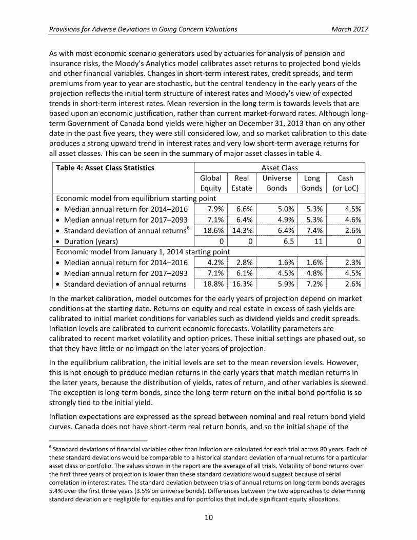
As with most economic scenario generators used by actuaries for analysis of pension and insurance risks, the Moody’s Analytics model calibrates asset returns to projected bond yields and other financial variables. Changes in short-term interest rates, credit spreads, and term premiums from year to year are stochastic, but the central tendency in the early years of the projection reflects the initial term structure of interest rates and Moody’s view of expected trends in short-term interest rates. Mean reversion in the long term is towards levels that are based upon an economic justification, rather than current market-forward rates. Although long-term Government of Canada bond yields were higher on December 31, 2013 than on any other date in the past five years, they were still considered low, and so market calibration to this date produces a strong upward trend in interest rates and very low short-term average returns for all asset classes. This can be seen in the summary of major asset classes in table 4.

Table 4: Asset Class Statistics Asset Class Global Equity

Real Estate

Universe Bonds

Long Bonds

Cash (or LoC)

Economic model from equilibrium starting point • Median annual return for 2014–2016 7.9% 6.6% 5.0% 5.3% 4.5% • Median annual return for 2017–2093 7.1% 6.4% 4.9% 5.3% 4.6% • Standard deviation of annual returns6 18.6% 14.3% 6.4% 7.4% 2.6% • Duration (years) 0 0 6.5 11 0 Economic model from January 1, 2014 starting point • Median annual return for 2014–2016 4.2% 2.8% 1.6% 1.6% 2.3% • Median annual return for 2017–2093 7.1% 6.1% 4.5% 4.8% 4.5% • Standard deviation of annual returns 18.8% 16.3% 5.9% 7.2% 2.6%

In the market calibration, model outcomes for the early years of projection depend on market conditions at the starting date. Returns on equity and real estate in excess of cash yields are calibrated to initial market conditions for variables such as dividend yields and credit spreads. Inflation levels are calibrated to current economic forecasts. Volatility parameters are calibrated to recent market volatility and option prices. These initial settings are phased out, so that they have little or no impact on the later years of projection.

In the equilibrium calibration, the initial levels are set to the mean reversion levels. However, this is not enough to produce median returns in the early years that match median returns in the later years, because the distribution of yields, rates of return, and other variables is skewed. The exception is long-term bonds, since the long-term return on the initial bond portfolio is so strongly tied to the initial yield.

Inflation expectations are expressed as the spread between nominal and real return bond yield curves. Canada does not have short-term real return bonds, and so the initial shape of the

6 Standard deviations of financial variables other than inflation are calculated for each trial across 80 years. Each of these standard deviations would be comparable to a historical standard deviation of annual returns for a particular asset class or portfolio. The values shown in the report are the average of all trials. Volatility of bond returns over the first three years of projection is lower than these standard deviations would suggest because of serial correlation in interest rates. The standard deviation between trials of annual returns on long-term bonds averages 5.4% over the first three years (3.5% on universe bonds). Differences between the two approaches to determining standard deviation are negligible for equities and for portfolios that include significant equity allocations.


11

inflation expectation curve in the market calibration reflects economic forecasts for short-term inflation and the spread between Canadian nominal and real return bond yields for long-term inflation. The mean reversion level for the inflation expectation curve is the same for all countries. Rates of inflation in the model include an independent stochastic component, in addition to fluctuations directly linked to the inflation expectation curve. The median inflation rate for the first three years of projection is 1.3% per year for the market calibration and 2.5% per year for the equilibrium calibration. The average standard deviation of annual inflation during the first three years is 1.5% for both scenario sets.

The distribution of one-year returns for an asset class does not follow the normal distribution and is not independent of returns for other asset classes or other years. Consequently, the usual statistical relationships amongst economic variables might hold approximately, but not precisely. For example, simulated multi-year returns for a portfolio that includes both equity and bonds will have a mean and variance different from the weighted average of the means and variances of the component asset classes, multiplied by the number of years. These differences due to dependencies and assumptions about the distribution of results are key to the effectiveness of an economic model.

Dealing with Expected Trends If the going concern discount rate is set by reference to equilibrium conditions or by reference to long-term expectations even when bond yields are expected to rise, then most stochastic trials will have intervaluation investment returns lower than the discount rate. For example, if going concern liabilities are determined using a 6% discount rate because this is the equilibrium rate of return on a balanced portfolio but the economic scenario generator produces median investment returns for the first three years of 2.5% per year, then the median result will be a 10.6% investment loss after three years (i.e., 1.063/1.0253-1).

The problem with using fixed long-term expectations to establish funding targets for pension plans is even more pronounced when we consider provisions for adverse deviations. Figure 1 shows the outcome of 10,000 trials from the economic scenario generator, with a traditional asset mix of 60% equities and 40% bonds.

Figure 1: Frequency Distribution of Portfolio Returns


12

In the equilibrium trials, the median annual rate of return is 6.80%, and 90% of the trials produce a three-year average rate of return greater than -1.85%. This would suggest that a margin of 29% (i.e., (1+6.80%

1−1.85%)3 − 1) would have a 90% chance of overcoming any investment

losses. But if this 29% margin were applied to the market trials, then it would give only an 80% chance of overcoming losses. The risk of investment losses greater than the margin would be twice as big as intended. If higher confidence is required (for example the 97.5% confidence level required for New Brunswick target benefit plans), then bias in the going concern discount rate can shift the tail of the distribution even more dramatically7.

Since we are attempting to determine a PfAD that achieves a given likelihood of full funding, rather than the likelihood of full funding given a predetermined PfAD, the effect of bias in the best estimate assumptions will not seem as dramatic as this. Rather than shifting the outcome further into the tail of the distribution, bias will simply be added to the required PfAD. If a 6.8% discount rate is used based on equilibrium conditions when the market expectation is a median 2.8% return, then a provision for expected adverse deviations of 12% will be required to achieve the target, over and above the provision for unexpected adverse deviations.

To circumvent the problem of short-term expectations that differ from long-term expectations and focus our attention on unexpected adverse deviations, we establish expected returns and liabilities at the next valuation date by reference to the median of the economic scenario generator, rather than by reference to a long-term expected rate of return. An equivalent way of thinking about this approach is to say we set a select and ultimate going concern discount rate, with a discount rate for the first three years reflecting the expected returns for that period and a discount rate applicable thereafter reflecting the expected returns during the fourth and subsequent years.

This approach is critical to the conclusion that PfADs do not need to be adjusted as market expectations for interest rates change. Best estimate assumptions must be unbiased as of the effective date of the valuation. Otherwise, a provision for unexpected adverse deviations will fail to address the expected short-term deviations from assumptions.

Changes in Best Estimate Going Concern Assumptions In practice, actuaries do not use select and ultimate going concern discount rates. If they use a single level discount rate that gives the same funding target at the current valuation date as the select and ultimate discount rates derived from an economic scenario generator and adjust the discount rate at each valuation, then the expected reduction in liabilities from rising interest rates will offset the expected loss on investments. These two intervaluation events would appear as separate entries in a reconciliation of the change in funded position, but they are two sides of the same coin.

In order to determine the PfAD that will meet a given target, we compare percentiles of the distribution of the combined investment, inflation, and economic assumption gain or loss, rather than considering these factors separately. We have found that, with this approach, the PfADs derived from the market calibration are remarkably similar to the PfADs from the

7 Frisen, J., “The ups and downs of stochastic modelling,” Benefits Canada, January 19, 2016, http://www.benefitscanada.com/uncategorized/the-ups-and-downs-of-stochastic-modelling-75708.

http://www.benefitscanada.com/uncategorized/the-ups-and-downs-of-stochastic-modelling-75708


13

equilibrium calibration. For example, figure 2 shows three-year economic gains and losses for a plan with a traditional balanced investment portfolio (60% equity, 40% bonds). The additional volatility that arises from adjusting the discount rate by 100% of the change in long bond yields is negligible. With a heavier allocation to bonds and a better match between bond duration and pension duration (so-called “liability-driven investing”), figure 3 shows the effect of adjusting discount rates for changes in market bond yields can largely offset the investment gains and losses. In the absence of assumption changes, the distribution of changes in funded status is the same as the distribution of investment returns, plus or minus any short-term bias in the going concern discount rate.

Figure 2: Distribution of Economic Gains (and Losses) with Traditional Asset Mix

Figure 3: Distribution of Economic Gains (and Losses) with Liability-Driven Asset Mix


14

The best estimate actuarial assumptions considered in this research paper are the expected return on assets (the discount rate) and the rate of inflation. Both are determined by reference to the median of trials from the economic scenario generator, as at the next (not the current) valuation date. This can be illustrated using the average rates of return on long-term bonds shown in table 4 above. When using the January 1, 2014 market calibration, the funding target for January 1, 2017 reflects a best estimate return on long-term bonds of 4.8%, rather than the equilibrium level of 5.3% or a lower average expectation as of January 1, 2014 that takes account of the short-term expected return of 1.6%. Adjustments to liabilities as at January 1, 2017 for each trial reflect differences in long-term bond yields and long-term inflation expectations between the median and the individual trials.

The approach we have used to adjust the best estimate actuarial assumptions in each individual trial reflects the simulated outcomes available in the model, accepted actuarial practice for setting discount rates, and the objective of assessing the adequacy of PfADs. In a narrow sense, we are attempting to anticipate the change to a best estimate going concern discount rate and inflation rate that an actuary would make if he or she were using this asset model and the model were recalibrated according to rules consistent with the model’s internal logic. To do otherwise would introduce bias into the results.

In reality, decisions about best estimate economic assumptions and about calibration of an economic scenario generator are not automatically linked to market events. A great deal of judgment is involved in deciding how a change in market conditions will affect future returns, especially for equities. Moreover, an economic scenario generator that has been designed for a different purpose such as guiding asset mix or setting reserves for non-indexed insurance products might not perform well as a predictor of median real pension fund returns.

Inflation Rate The actuarial assumption for the rate of inflation is taken to be the average of differences between real and nominal bond spot rates over the years after January 1, 20178. Or, more precisely, there is an unexpected adjustment to liability due to a change in this statistic different from the median.

While short-term inflation forecasts are a key factor in the calibration of short-term real and nominal bond yields, longer bond yields are calibrated to the actual yields on long-term bonds. Pension actuaries would consider these same factors in their selection of an inflation rate.

The role of the inflation rate relative to the rate of return on investments depends upon the plan design.

• In a flat benefit plan with no post-retirement indexation and no anticipation of improvements to the flat benefit rate, inflation plays no role in the calculations. Only the nominal rate of return matters.

• At the other extreme, in a final earnings pension plan with full indexation of pensions, plan benefits increase more or less in lockstep with the Consumer Price Index. Only the real rate of return matters.

8 We use a simple average of the spot rate differences for the years 2017 through 2036, to capture the part of the curve that is most relevant to final average earnings and post-retirement indexation without placing undue weight on the long or short end of the curve.


15

• For plans that provide partial inflation protection prior to retirement through a final or career average earnings formula but do not provide inflation protection after termination of employment, both the nominal rate of return and the inflation rate are important. Discount Rate

The Canadian Institute of Actuaries provides guidance to pension actuaries on the factors to consider when setting going concern discount rates9. With the building block approach, the best estimate expected return will be a blend of the expected returns for each asset class, plus adjustments for diversification, investment management fees, and active management. If the term of the liabilities is longer than the term of the bonds in the portfolio, then there will be an additional adjustment for reinvestment in new fixed income securities.

If a frozen pension plan has been invested in a portfolio of bonds that replicates the expected benefit cash flows, then the discount rate used to determine expected return on assets should track the yield on the bond portfolio precisely. Even in the absence of absolute matching, the guidance for actuaries permits the selection of a going concern discount rate based on bond yields on the valuation date. This market-based approach is akin to the solvency valuation basis discussed below, and serves as a useful benchmark for evaluating other approaches to adjusting going concern discount rates.

The PfAD calculations presented in this report reflect adjustments to going concern discount rates according to the asset mix.

• The expected return on fixed income investments (including universe bonds, long-term bonds, and cash) varies according to the average yield on long-term bonds.

• The expected return on other investments (including global equity and real estate) varies according to the change in the inflation assumption. That is, the expected real rate of return is assumed to remain constant.

For example, if 60% of the assets are invested in equities and real estate, with the remaining 40% invested in bonds and cash, the increase (or decrease) in the going concern discount rate at January 1, 2017 for a specific trial would be the following:

• 60% of the increase (or decrease) in the assumed inflation rate; plus • 40% of the excess (or shortfall) of the long-term bond yield for the specific trial over the

median of all trials. Some of the asset mixes involve negative allocations to cash (overlay strategies). These negative allocations are deducted from the allocation to equity and real estate for the purpose of adjusting discount rates.

We did not consider changes in the adjustment for diversification that would arise in the economic scenario generator as a result of changes in the volatility of returns (dynamic increases in volatility would produce a larger rebalancing premium).

The rationale and alternatives to these choices are discussed in appendix A. 9 Canadian Institute of Actuaries, “Revised Educational Note – Determination of Best Estimate Discount Rates for Going Concern Funding Valuations,” December 7, 2015, accession number 215106, http://www.cia-ica.ca/publications/publication-details/215106.

http://www.cia-ica.ca/publications/publication-details/215106


16

Solvency Basis Information on the cost of settling benefits in a hypothetical wind-up is included alongside the assessment of going concern PfADs to illustrate how a going concern PfAD might enhance security of benefits in a plan wind-up situation. Details of the basis for determining the solvency position are included in appendix B.

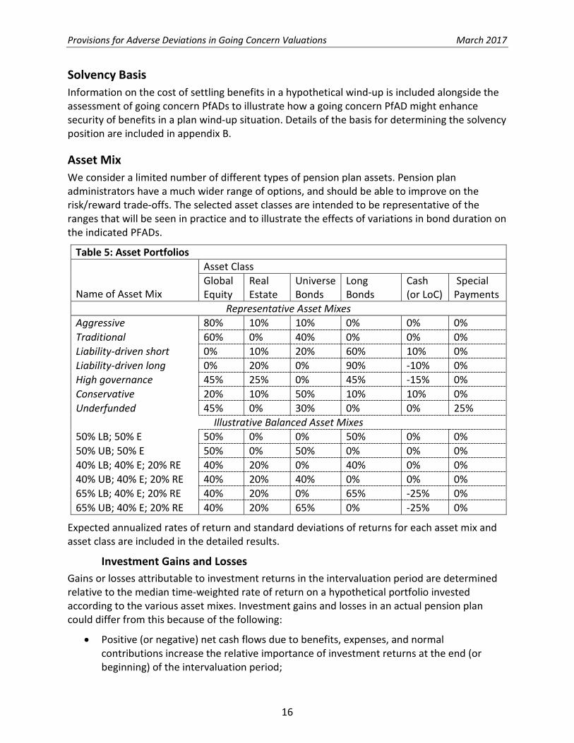
Asset Mix We consider a limited number of different types of pension plan assets. Pension plan administrators have a much wider range of options, and should be able to improve on the risk/reward trade-offs. The selected asset classes are intended to be representative of the ranges that will be seen in practice and to illustrate the effects of variations in bond duration on the indicated PFADs.

Table 5: Asset Portfolios Name of Asset Mix

Asset Class Global Equity

Real Estate

Universe Bonds

Long Bonds

Cash (or LoC)

Special Payments

Representative Asset Mixes Aggressive 80% 10% 10% 0% 0% 0% Traditional 60% 0% 40% 0% 0% 0% Liability-driven short 0% 10% 20% 60% 10% 0% Liability-driven long 0% 20% 0% 90% -10% 0% High governance 45% 25% 0% 45% -15% 0% Conservative 20% 10% 50% 10% 10% 0% Underfunded 45% 0% 30% 0% 0% 25%

Illustrative Balanced Asset Mixes 50% LB; 50% E 50% 0% 0% 50% 0% 0% 50% UB; 50% E 50% 0% 50% 0% 0% 0% 40% LB; 40% E; 20% RE 40% 20% 0% 40% 0% 0% 40% UB; 40% E; 20% RE 40% 20% 40% 0% 0% 0% 65% LB; 40% E; 20% RE 40% 20% 0% 65% -25% 0% 65% UB; 40% E; 20% RE 40% 20% 65% 0% -25% 0%

Expected annualized rates of return and standard deviations of returns for each asset mix and asset class are included in the detailed results.

Investment Gains and Losses Gains or losses attributable to investment returns in the intervaluation period are determined relative to the median time-weighted rate of return on a hypothetical portfolio invested according to the various asset mixes. Investment gains and losses in an actual pension plan could differ from this because of the following:

• Positive (or negative) net cash flows due to benefits, expenses, and normal contributions increase the relative importance of investment returns at the end (or beginning) of the intervaluation period;


17

• The present value of established special payments will decline over the intervaluation period, reducing interest rate risk and increasing investment risks (except to the extent that special contributions are invested in fixed income investments with a similar term); and

• Rebalancing of the portfolio could occur more or less frequently than annually. These differences are not material to the results. In an extreme case, if a very mature plan were to pay out 10% of the plan assets each year, investment gains and losses and indicated PfADs would be about 15% bigger when expressed as a percentage of the best estimate liabilities at the next valuation date10. If the PfAD were expressed as a percentage of the best estimate liabilities at the current valuation date, the PfAD would be about 15% smaller. That is, the PfAD should be expressed as a percentage of the average intervaluation liabilities, rather than the starting or ending liabilities, when intervaluation net cash flows are significant.

Disregarding net cash flows and special payments over the three-year time horizon also simplifies the manner in which required PfADs are calculated and funded. The distribution of the ratio of the plan’s assets (including the expected present value of remaining special payments) to the plan’s actuarial liabilities (including the PfAD) is the same regardless of the level of the PfAD. The PfAD required to achieve a given confidence level can be calculated by determining the asset and liability gains and losses in percentage terms and using the combined percentage to determine the PfAD.

Typical Pension Plan Characteristics Pensioner liability as a percentage of total liability varies widely between pension plans. For a new pension plan or a pension plan that has always purchased annuities for retiring employees, this percentage could be as low as zero, while for a pension plan that has been closed for an extended period, it could approach 100%.

While there are differences in active liability duration attributable to the benefit accrual formula (flat benefit or earnings-related), availability and utilization of survivor pensions, bridge benefits, and the history of demographic growth and plan changes, none of these are large and none is as important as the mix of pensioners and other membership categories (including active members). Plan design (aside from indexation) does not determine the interest rate sensitivity of pensioner liabilities. The presence of inflation protection, especially after retirement, is a key distinguishing plan design feature to be considered in the establishment of PfADs.

Based on analysis of pension plan statistics and variations in plan characteristics, four cases representative of the full range of diversity of pension plans were considered. These are shown in table 6.

10 The assets exposed to risk during the first year would be 125% of projected assets, declining to 115% in the second year and 105% in the third year. The three-year investment gain or loss would be

(i1 - i)*125% * (1 + i2) * (1 + i3 ) + (i2 – i)*115% * (1 + i3 ) + (i3 - i) * 105% The extra weight on earlier years does not significantly alter the distribution of gains and losses.


18

Table 6: Specimen Pension Plan Designs

Average Mature Young Public Sector

Plan features Open career

average

Closed flat benefit, bridge

Open non-indexed final average

Open indexed

final average

Members other than pensioners • Duration11 • Effect of 1% inflation surprise • Effect of 1% increase in

expected future inflation

17.4 0.4%

2%

17.2 Nil

Nil

22.2 0.9%

8%

19.712 0.9%

20%

Pensioners • As a percentage of total • Duration • Effect of 1% increase in

expected future inflation

50% 8.6

Nil

80% 8.0

Nil

20% 8.6

Nil

50% 9.4

10%

Overall duration 13.1 9.9 19.6 14.6

Results Provisions for adverse deviations indicated by various asset mixes, plan characteristics, and target confidence levels are presented in tabular form in appendix A. An explanation of the values shown in the appendix is provided here.

Average Plan For example, the PfAD value shown in appendix A for the following situation is 21.2%:

• The specimen average plan (open career average, 50% pensioners, non-indexed); • A traditional asset mix (60% equities, 40% bonds); • An 85% confidence level; and • Equilibrium calibration of the model.

This is illustrated in figure 4. Each of the thousand points represents the outcome of one stochastic trial; 850 of the points fall above the green line and 150 fall below this line. The orange full funding line (assets = best estimate liabilities) lies 21.2% above the green line. This means that if funding is in place so that assets are expected to equal 121.2% of liabilities at the 11 Duration is presented here as D(5.25%), the duration at 5.25%. It measures the effect of a 1% reduction in the discount rate from 5.75% to 4.75%. The unexpected change in liability when the initial best estimate expected return on assets i is different from 5.75% or the unexpected decrease Δi is different from 1% is e Δi ∙D(i- Δi /2)-1, where

D(i- Δi /2) = D(5.25%)∙ [1+7∙(5.25%-(i- Δi/2))] The logarithmic convexity factor of 7 is applied to liabilities for pensioners and other members separately. For a fuller discussion, refer to Research paper on discount rate sensitivities in pension plans. 12 The duration statistics for indexed pensions are about 0.2 years lower when the economic scenario generator is calibrated to January 1, 2014 market conditions, because of lower expected inflation.



19

end of a three-year period (with 50% of the trials producing a better outcome and 50% producing a worse outcome), then 85% of the trials will produce assets greater than 100% of liabilities.

Figure 4: Equilibrium Model Outcomes for Average Plan with Traditional Asset Mix

Similarly, 500 of the points fall above the orange line, 750 of the points fall above the grey line, and 950 of the points fall above the dark blue line.

The range of asset gains and losses reflects a standard deviation for the traditional asset mix of 11.2%. Since the standard deviation of equity returns shown in table 4 is 18.6%, most of the investment risk can be attributed to the 60% allocation to equities. (As noted on table 4, standard deviations are calculated across 80 years for each trial, and the statistics shown are the averages of standard deviations for all trials).

In this situation, solvency (hypothetical wind-up) liabilities are, on average, 110.4% of going concern liabilities, because the discount rates used to measure solvency are lower than the best estimate expected rate of return on assets. Results of individual trials vary because of variations in the shape of the yield curve, credit spreads, and expected inflation. Before adding a PfAD to the assets, the ratio of solvency assets to liabilities lies in a range of 67% to 119% in 900 out of 1,000 stochastic trials. That is, with a funding target set to 100% of going concern liabilities, there is a 5% chance that assets would be less than 67% of the solvency liabilities and a 5% chance they would be more than 119%.


20

If a PfAD were in place to provide assets equal to 121.2% of projected going concern liabilities and an 85% likelihood of full funding on a going concern basis, then

• The range of solvency ratios shifts upwards: 900 out of 1,000 trials would have a solvency ratio between 81% and 145%; and

• The solvency ratio is at least 100% in 70.4% of the trials.

Thus, although a PfAD that targets an 85% likelihood of full going concern funding improves the likelihood of full solvency funding, it does not guarantee solvency or even provide an 85% likelihood of full funding on a solvency basis. Figure 5 illustrates the relationship between the going concern funded ratio and the solvency funded ratio, before addition of a PfAD to the assets. Points above the red line represent the 704 out of 1,000 stochastic trials in which the 21.2% PfAD would be enough to make the plan solvent.

Figure 5: Funding Ratios for Average Plan with Traditional Asset Mix

Mature Plan

Once a plan has been closed to new entrants and the benefits for existing members have been frozen, the liability for pensioners will become an increasing proportion of the total. The opportunity to reduce risk through liability-driven investing will become more realistic. With this situation and the equilibrium model calibration, the PfAD required for an 85% confidence level is reduced to 3.0%. This is mostly because of the strong correlation between assets and liabilities, as illustrated in figure 6.

Outcomes below this line would have solvency ratios less than 100%, even with a going concern PfAD set at the 85% confidence level.


21

Figure 6: Equilibrium Model Outcomes for Mature Plan with Liability-Driven Asset Mix

The heavy allocation to bonds means that the expected return on assets will move closely in tandem with the cost of purchasing annuities, and so the likelihood of a large solvency deficit emerging is also reduced. The correlation coefficient between asset returns and liability adjustments due to discount rate changes is 94%. This is illustrated in figure 7.


22

Figure 7: Funding Ratios for Mature Plan with Liability-Driven Asset Mix

If funding were in place to provide assets equal to best estimate going concern actuarial liabilities plus a 3.0% PfAD, then the solvency ratio in the mature plan would fall between 93% and 105% in 90% of the trials (as compared to the range from 81% to 145% for the average plan with a 21.2% PfAD). Note that the lowest solvency ratios in the graph are much higher than the solvency ratios shown above for the average situation, but this is offset by a much smaller going concern PfAD. The 3% PfAD is only sufficient to provide full funding on a solvency basis in 32.3% of the trials.

Public Sector Plan Membership in defined benefit pension plans in Canada is dominated by a small number of very large public sector pension plans. These plans provide benefits that are linked to inflation (through earnings adjustments prior to retirement and pension adjustments after retirement). Typically, investment strategies are more sophisticated than can be adopted by smaller, private sector defined benefit pension plans, including derivative strategies and private infrastructure investments. With this situation and the equilibrium model calibration, the PfAD indicated for an 85% confidence level is 21.7%. Although inflation protection adds to the risk when a conservative or (non-indexed) liability-driven investment strategy is used, the results with the traditional asset mix or a high governance asset mix are similar to those shown above for the average non-indexed plan.


23

Figure 8: Equilibrium Model Outcomes for Public Sector Plan with High Governance Asset Mix

Because of the inflation risk premium embedded in indexed annuity prices, the range of solvency funding ratios is lower than for other plan designs, as illustrated in figure 9.

Figure 9: Funding Ratios for Public Sector Plan with High Governance Asset Mix


24

Observations 1. Comparison to Other Sources

The 2013 CIA task force report shows required PfADs with a 75% or 90% likelihood of full funding, a three-year time horizon, and a range of asset mixes and plan maturity levels. We understand the target reserve levels prescribed under Québec pension funding regulations13 reflect an 85% likelihood of full funding, a three-year time horizon, and a range of bond maturity levels. As compared to the results from our model with comparable parameters, some of the results from these sources are lower and others are higher. The PfADs reported here for asset mixes that have a significant allocation to equities are substantially higher. While we do not have enough detailed information on model inputs to conduct a complete reconciliation of the differences, it would appear that

• Lower equity risk in the 2013 report is in part due to a conservative best estimate assumption for return on equities;

• The Québec factors reflect adjustments to discount rates equal to 100% of the change in long-term bond yields and negligible inflation risk; and

• Other differences could be explained by lower interest rate volatility, higher equity volatility, or a smaller duration mismatch (the difference between the duration of the bond universe and the duration of specimen pension plan liabilities) in the current model.

Economic scenario generators are constructed to achieve specific objectives, such as optimizing risk/return trade-offs in investment policies or establishing a fair market price for embedded options in financial contracts. Judgment is required to decide on the extent of future investment volatility and linkages between factors. Differences in outcomes are not unexpected, and are entirely within the range of reasonability. The results shown in the 2013 task force report and this report serve to highlight the relationship between the need for a PfAD and such factors as initial market conditions and plan design. Comparison of results from different reports and different economic scenario generators will give an indication of the range of results that could arise from a reasonable range of model parameters.

2. Importance of Model Parameters Different results can be attributable to variations in the application of an economic scenario generator as well as variations in the way the model is constructed. We found we would arrive at materially larger PfADs if the equity allocation is handled differently. The 2013 task force report derived equity returns as a blend of 50% Canadian equity (shares in companies with their primary listing on the Toronto Stock Exchange), 25% U.S. equity (shares in companies with their primary listing on a New York stock exchange) and 25% EAFE equity (shares in companies with their primary listing in a developed market in Europe or the Far East). As shown in table 1, our hypothetical equity investments have a smaller allocation to the Toronto Stock Exchange and include an allocation to emerging markets.

By assuming broad geographical diversification and annual rebalancing to the original allocation percentages, our application of the economic scenario generator produces lower volatility and 13 The target level for the so-called “stabilization provision” under section 125 of the Québec Supplemental Pensions Act can be found in section 60.6 of the regulation respecting supplemental pension plans (chapter R-15.1, r.6). http://www.rrq.gouv.qc.ca/en/services/publications/rcr/loi_reglements/Pages/loi_reglement.aspx

http://www.rrq.gouv.qc.ca/en/services/publications/rcr/loi_reglements/Pages/loi_reglement.aspx


25

higher returns than would result from allocation to a single geography or to a global equity portfolio without rebalancing by geography. If we had simply assumed a 50% allocation to U.S. equities and a 50% allocation to non-U.S. equities, the standard deviation of equities would have been 21.0% instead of 18.6% as shown in table 4, and the PfAD required for an 85% likelihood of full funding for an average plan and a traditional asset mix would have been 23.9% rather than 21.2%. Simply changing the way currency and geographical risk is managed within the equity component of the economic scenario generator can increase the indicated PfAD by 13%.

In general, it will be important to use the same parameters and the same economic scenario generator or other process to determine a PfAD and to determine the expected return on assets and expected rate of inflation. A larger PfAD might be required if the expected return on assets is determined without regard to current market conditions at the valuation date or there is no intention to adjust actuarial assumptions from one valuation to the next. On the other hand, if the benefits of active rebalancing or currency hedging are not fully anticipated, the PfAD might be overstated.

Liability-driven investing (using bonds that match the payment characteristics of the benefits) can be an extremely effective way to reduce pension risk relative to the risks in traditional investment strategies. These strategies are straightforward when plans are non-indexed and mature. The approach to reducing the need for PfADs in benefits for active employees or benefits that are indexed to inflation is not as obvious. When liability-driven investing is used to reduce funding volatility, matching the duration of bonds to the duration of liabilities can further reduce the risk. This is reflected in the target reserve levels prescribed under Québec pension funding regulations. Québec targets are increased by 0.08% for every 1% reduction in the match between liability duration and the duration of fixed income assets. For example, the target “stabilization reserve” with 50% of assets allocated to fixed income is 11% when the duration of fixed income assets is 75% of liability duration and increases to 15% when the duration of fixed income assets is 25% of liability duration. Our model produces similar results when the allocation to fixed income is high and the benefits are non-indexed. However, when these conditions are not met, the effect of duration matching is much smaller or non-existent. It would appear, at least in the economic scenario generator we are using, that the only way to dampen the effect of the worst equity returns is through asset classes that are not correlated with equities, and long-term bonds suffer from correlation with equities.

3. Funding Levels The effect of underfunding is to reduce the required PfAD in proportion to the funding ratio. All else being equal, the PfAD for a non-indexed plan that is expected to be 75% funded at the next triennial valuation will be slightly less than 75% of the PfAD for the same plan with the same mix of investments and total investments expected to equal 100% of the expected liabilities at the next triennial valuation. This is because the value of scheduled special payments varies with the discount rate. A similar result could presumably be obtained for indexed plans if the scheduled special payments were also indexed. The effect of a funding target that is different from full funding with a PfAD is similar to underfunding. In particular, if the PfAD were excluded from the target level of assets, then


26

investment gains and losses attributable to the PfAD would be eliminated, and the indicated PfAD would be smaller, by roughly the reduction in the PfAD. In the example of an average plan with a traditional asset mix, the indicated PfAD cited above is 21.2%. If no funding were required for the PfAD, then elimination of the PfAD on the PfAD would reduce the indicated PfAD to about 17%.

4. Investment Strategy Investment strategies with greater expected returns generally (but not always) bear extra risk. When the indicated PfAD is expressed as a margin in the discount rate, rather than as a percentage of best estimate liabilities, it often comes very close to wiping out the difference in expected returns between aggressive and conservative investment strategies. This is illustrated in table 7. Table 7: Discount Rate with Expected Rate of Return Adjusted for PfAD over 13-Year Duration

Expected Confidence Level

Return 75% 85% 95%

Asset Mix Conservative 5.82% 5.6% 5.4% 5.2%

Traditional 6.60% 6.0% 5.6% 5.0% Underfunded 6.60% 6.1% 5.9% 5.4% Aggressive 7.08% 6.2% 5.7% 4.7% LDI short 5.37% 5.2% 5.2% 5.0% LDI long 5.71% 5.6% 5.5% 5.3% High governance 6.93% 6.3% 6.0% 5.4%

Three somewhat related sources of unanticipated changes in funded position are considered in this report:

• Equity risk due to investment in assets with higher expected returns; • Interest rate risk due to a mismatch between the timing of payment of liabilities and the

timing of anticipated cash flows from investments; and • Inflation risk.

As noted above, liability-driven strategies can be effective in producing very low levels of risk for non-indexed, mature plans. In other situations, strategies involving equity risk are less unattractive:

• For indexed plans, a higher level of risk is almost inevitable due to the challenges of hedging inflation risk, and equity investing might not add significantly to risk levels.

• For less mature plans, interest rate risk cannot be adequately addressed through matching fixed income instruments because the term of the liability is too long and the timing of future retirements is uncertain. 5. Effectiveness in Assuring Solvency

A best estimate going concern discount rate anticipates excess returns due to risky investments. The funding target is reduced before the risks have been taken and before the excess returns are earned. Thus, in the absence of a PfAD, a going concern funding target will


27

be smaller than the price of settling a pension plan’s liabilities. As illustrated in table 7, a PfAD can largely eliminate the gap due to this anticipated risk premium. A going concern funding target including a PfAD can do a good job of maintaining solvency in an equilibrium environment and for plans with a significant element of future salary growth in total going concern liabilities, but does a poor job for other types of plans and in a low interest rate environment. When the spread between current interest rates and long-term expected returns is larger than normal, solvency liabilities will be much larger than going concern liabilities. Although the market calibration of the model anticipated some narrowing of the gap during the first three years after January 1, 2014, a significant gap still remained in most of the trials, and so results on that basis show much poorer solvency performance.

Areas for Further Research This research paper considers funding risk over a single, relatively short, time horizon. The true test of a funding regime is its ability to sustain a pension plan over the lifetime of the plan members. With all the complexities of amortization periods, valuation frequency, and changing membership, it is not practical to assess all of the variables in a single study. Possible extensions of this research that would shed light on the choices faced by regulators and plan sponsors include the following:

• Analysis of a dynamic allocation strategy that automatically adjusts risk as funding levels change;

• Quantification of risks due to statistical fluctuations in small pension plans, including o Pensioner mortality, o Late-career bonuses or pay increases in best average earnings pension plans, and o Representative plan-specific risks due to utilization of early retirement subsidies;

• Analysis of longer time horizons, within the context of one set (or a small number of sets) of rules for determining contributions and investment strategy;

• Estimation of indicated going concern PfADs for all existing single-employer pension plans based on Actuarial Information Summary data;

• Analysis of the gradual wind-down of the entire single-employer defined benefit pension system (including the risk of sponsor bankruptcy), to determine if plan members might be better served by going concern funding with moderate investment risk, rather than solvency funding with liability-driven investing; and

• Investigation of differences in results due to different economic scenario generators used by Canadian pension actuaries.


28

Appendix A: Alternative Approaches to Asset Class Expected Returns

Long-Term Bonds For a frozen, non-indexed plan, a portfolio of long-term bonds can provide cash flows that closely match the expected benefit payments. In the absence of defaults, this portfolio will produce an average return that matches the initial yield. While credit spreads do vary, the variation in credit spreads would significantly overstate variations in expected credit defaults for investment-grade, long-term bonds.

The average duration of a specific portfolio of bonds will decline with the passage of time, as bonds mature and are not replaced. For an open pension plan or a plan with a duration of liabilities longer than the duration of a long bond portfolio, this approach will not provide a close match to projected benefit payments. A portfolio that tracks an index (with new bonds added as they are issued and existing bonds removed when the term to maturity falls below 10 years) will have a more stable duration. This approach is more typical when long-term bonds are one asset class within a balanced portfolio. The expected return on this kind of bond portfolio will not necessarily track the initial yield. The return on bonds that are added to the portfolio over time will depend upon market yields at the time they are purchased.

Nonetheless, long-term bond yields are more stable than short-term yields and can be a better indicator of future returns than alternatives. Figure A1 shows 1,000 trials from the Moody’s economic scenario generator, calibrated to January 1, 2014 market conditions. Each point on the graph represents the outcome of one trial. This graph highlights the relationship between long-term bond yields at January 1, 2017 and average returns on long-term bonds for the 20 years from January 1, 2017 through December 31, 2036.

Figure A1: Distribution of Long Bond Returns


29

Universe Bonds and Cash Although yields on short-term fixed income investments do not always move in the same direction as longer term yields, they often do. The difference in yield between short-term and long-term government bonds can be thought of as a combination of the following:

• A term premium (an extra yield on longer term bonds to compensate for the extra uncertainty as to their liquidation value in the years prior to maturity); and

• A market forecast of future yields. To the extent fluctuations in long-term bond yields are due to fluctuations in expected future yields, it is appropriate to reflect these fluctuations in the expected return on shorter-term bonds and cash. Figure A2 illustrates that there has been a very close relationship between the yield on long-term bonds and the average return on bonds held by pension funds14.

Figure A2: Long Bond Yields and Lagged Bond Returns

This relationship is also present in the Moody’s economic scenario generator, as illustrated in Figure A3. In fact, long-term bond yields appear to be a better predictor of universe bond returns than universe bond yields.

14 Long-term government bond yields are reported by the Bank of Canada at http://www.bankofcanada.ca/wp-content/uploads/2010/09/selected_historical_v122487.pdf. The average return on bonds was calculated from reports by the Canadian Institute of Actuaries in its annual Report on Canadian Economic Statistics 1924–2015.

http://www.bankofcanada.ca/wp-content/uploads/2010/09/selected_historical_v122487.pdf

http://www.bankofcanada.ca/wp-content/uploads/2010/09/selected_historical_v122487.pdf

http://www.cia-ica.ca/docs/default-source/members/216066e.pdf?sfvrsn=0


30

Figure A3: Distribution of Universe Bond Returns

Equities We considered a variety of model statistics to indicate the change in expected return on equities. None is a particularly good indicator of equity returns. The high degree of volatility in equity returns overwhelms the predictive value of any particular statistic.

• Since the price of a stock is often expressed as the present value of future corporate earnings or dividends, it would seem reasonable to expect stock prices to reflect long-term interest rates. Unfortunately, this theoretical argument is not supported by positive historical correlation between bond returns and equity returns and is seldom reflected in the construction of economic scenario generators.

• The regular and increasing dividend payments from an equity portfolio could make equities suitable for securing the projected benefit payments from a pension plan. From this perspective, fluctuations in the market value are unimportant if the underlying dividend-paying capacity is unchanged. Thus, fluctuations in the dividend yield (or total cash yield, including share buy-backs and other cash distributions) could be a suitable indicator of appropriate adjustments to the expected return on equities. Unfortunately, like bond yields, this theoretical argument is not strongly supported by history or the output from the economic scenario generator.

• The specifications for the Moody’s economic scenario generator define equity returns relative to the return on cash. Stock traders buy or sell stocks on margin: they need to outperform the return on cash just to break even, and the “equity risk premium” is often defined relative to cash returns. Varying the expected return on equities according to the yield on short-term fixed income investments would be akin to assuming this equity risk premium does not vary over time.


31

• After a significant stock market decline, there is often an expectation of recovery. This belief in mean reversion is widely held, but not supported by evidence15. On the contrary, the Moody’s economic scenario generator includes a small element of momentum—positive serial correlation of equity returns.

• Corporate bond yields are expressed as the yield on a government bond with a similar term or duration plus a credit spread to reflect the reduced liquidity and increased risk of default attributable to the particular issuer and debt covenant. Credit spreads can increase significantly during a downturn in equity markets, but this does not translate into overall correlation or predictive power.

• There is some evidence that price-to-earnings (P/E) ratios have predictive power for future stock market returns16, but this statistic was not available in our economic scenario generator data.

The effect of alternative approaches to adjusting going concern discount rates depends on the asset mix and the inflation sensitivity of the plan’s benefits. Using a metric aligned with solvency will produce going concern experience adjustments very similar to the solvency adjustments. Figure A4 and figure A5 illustrate the relationship between the going concern funded ratio and the solvency (hypothetical wind-up) funded ratio for a mature plan (flat benefit, non-indexed pension, 80% pensioners, overall duration 9.9 years) with a traditional asset mix (60% global equities, 40% Canadian universe bonds). The graph on the left shows the effect of adjusting the going concern discount rate by 100% of the changes in the long bond yield, while the graph on the right shows the effect of adjusting the going concern discount rate by 40% of the changes in the long bond yield (i.e., adjusting the expected return on bonds but not the expected return on equities).

Figure A4: 100% of Changes in Long Yield Figure A5: 40% of Changes in Long Yield

Notice the following:

15 Office of the Superintendent of Financial Institutions Canada, “Evidence for Mean Reversion in Equity Prices,”, March 2012,. http://www.osfi-bsif.gc.ca/Eng/Docs/mnrv.pdf. 16 The Vanguard Group Inc., “Forecasting stock returns: What signals matter, and what do they say now?,” October 2012. https://personal.vanguard.com/pdf/s338.pdf.

http://www.osfi-bsif.gc.ca/Eng/Docs/mnrv.pdf

https://personal.vanguard.com/pdf/s338.pdf


32

1. The average going concern funded ratio is 100%, since no PfAD has been included. The effect of a PfAD would be to shift all the points on the graph upwards and to the right by the same amount.

2. The relationship between the going concern funded ratio and the solvency funded ratio is not perfect, even when the going concern discount rate is adjusted by 100% of the change in long-term bond yields. This is because the mixture of bonds used to establish the yield on long-term bonds has a slightly different pattern of payments and credit risks than the spot rates used to establish the solvency liabilities.

3. A fixed expected return on equities leads to a greater divergence of going concern and solvency results.

Although it is not obvious from the graphs, the required PfADs are not very different. Appendix A (adjusting the going concern discount rate by 40% of the changes in the long bond yield and 60% of the change in expected inflation) shows that a 12.8% PfAD provides a 75% chance of full funding, a 21.5% PfAD provides an 85% chance of full funding and a 38.0% PfAD provides a 95% chance of full funding. The corresponding PfADs are

• 12.1%, 19.7%, and 35.0% when adjusting the going concern discount rate by 100% of the changes in the long bond yield; and

• 12.7%, 20.5%, and 37.0% when adjusting the going concern discount rate by 40% of the changes in the long bond yield.

Other approaches to adjusting the expected return on equities (including using the yield on universe bonds, the inflation rate, or the dividend yield) also produce similar PfADs and a relationship between solvency and going concern similar to the graph on the right (with no adjustment to the expected return on equities).

A liability-driven investing strategy produces a much smaller dispersion of simulated results, as illustrated in figure A6 and figure A7. As in figures A4 and A5, the two graphs have identical dispersion of solvency results, but the going concern results differ because the graph on the left uses 100% sensitivity of discount rates to long-term bond yields, while the graph on the right uses a fixed going concern discount rate.

Figure A6: 100% of Changes in Long Yield Figure A7: Fixed Discount Rate

For plans with benefits linked to inflation, fixing the real expected return on equities rather than the nominal expected return produces less volatility and smaller PfADs. Figure A8 and


33

figure A9 illustrate the relationship between the going concern funded ratio and the solvency (hypothetical wind-up) funded ratio for the specimen public sector pension plan (best average earnings, fully indexed pensions, 50% pensioner liability, overall duration 14.6 years) with a high governance asset mix (45% global equities, 45% Canadian long-term bonds, 25% real estate offset by 25% short-term debt). The graph on the left shows the effect of adjusting the going concern discount rate by 45% of the changes in the long bond yield, while the graph on the right shows the effect of adjusting the going concern discount rate by 45% of the changes in the long bond yield and 55% of the changes in the inflation assumption (i.e., holding the expected return on equities constant in real terms rather than nominal terms).

Figure A8: 45% Long Yield Figure A9: 45% Long Yield + 55% Inflation

Although the correlation of equity returns and inflation is modest, both in historical records and in economic scenario generators, in the absence of a clear justification for varying expected equity returns, it is reasonable to hold expected equity returns constant. For pension plans with benefits fully linked to inflation, this would be expressed in real terms. For pension plans without inflation protection, the choice is unimportant.

Real Estate and Infrastructure Alternative investments, including direct investment in real estate and infrastructure projects, are often cited as appropriate investments for pension plans because they provide stable income over a long term. They do not trade in an active market, and so their appraised value is used in pension fund financial statements. This appraised value relies on a capitalization rate that evolves over time somewhat independently of bond yields.

In economic scenario generators, inclusion of real estate in a pension plan asset mix provides improved expected returns relative to bonds with diversification of risk relative to equities.


34

Appendix B: Solvency

Since 1986, most Canadian jurisdictions have required funding on the basis of both a going concern valuation and a hypothetical wind-up (HWU) valuation. The HWU liability for a pension plan is the cost of settling vested benefits, typically through a group annuity purchase and payment of commuted values. The assets used in a HWU valuation are measured at their liquidation value. This metric of funded status is a mark-to-market measure and is more volatile than the funded status on a going concern basis unless the asset mix is chosen with settlement costs in mind.

Regulatory standards have often modified the hypothetical wind-up basis to permit smoothing or to include or exclude certain benefits. The regulatory basis is usually called a solvency valuation. As interest rates have declined and pension plans have matured, solvency valuations have grown into the primary determinant of pension plan contributions.

Many commentators view the ability to pay all benefits when a plan actually winds up to be the only measure of funding that really matters. While a pension plan is ongoing, pre-funding helps to align cash costs with the accrual pattern of benefits, but the absolute level of invested assets does not affect the benefits. The addition of solvency valuations to minimum contribution requirements was intended to improve confidence that members would receive all their benefits after a plan winds up. In fact, solvency funding has not guaranteed this outcome. Amortization and smoothing of solvency deficits, along with inter-valuation market fluctuations have continued to lead to underfunding in wound up pension plans since 1986.

Typically when a pension plan is wound up, active plan members not yet eligible for an immediate pension are offered a choice between a commuted value and a deferred annuity. Pensioners are not offered the commuted value option. Active members eligible for an immediate pension at the time of the wind-up and deferred pensioners may or may not be offered commuted values, depending on plan provisions and regulatory requirements. For the purpose of a HWU valuation of an ongoing pension plan, actuaries will make an assumption about the proportion of active plan members who will elect commuted values. A common simplifying assumption is that 100% of active plan members not eligible for an immediate pension would elect lump sums and all other plan members would receive their HWU benefits through a group annuity purchase. Since the members eligible for an immediate pension are older and have longer service, they typically represent a large proportion of the total active liability. The split of active HWU liabilities between commuted values and group annuities is typically not reported in valuations or government filings.

Annuity Guidance The Canadian Institute of Actuaries provides guidance to pension actuaries on the cost of group annuities, based on a quarterly survey of insurance companies17. This is commonly called the annuity proxy because it is used as a proxy for actual annuity quotations in solvency and HWU

17 Quarterly guidance is posted at http://www.cia-ica.ca/publications/guidance. Final guidance for the first quarter of 2014 can be found in Assumptions for Hypothetical Wind-up and Solvency Valuations with Effective Dates Between December 31, 2013 and December 31, 2014, document 214039, Committee on Pension Plan Financial Reporting, April 2014.

http://www.cia-ica.ca/publications/guidance



35

valuations. During 2014 and 2015, the guidance was expressed in terms of the yield spread over Government of Canada long-term bonds (CANSIM v39062), together with the UP94G mortality table. The spread varies according to the duration of the pension liabilities. For example, for HWU valuations with a valuation date during the first quarter of 2014, the guidance for non-indexed annuities was as follows:

Table B1: Solvency Guidance Effective December 31, 2013

Illustrative block Duration based on

3.83% discount rate Spread above unadjusted

CANSIM V39062 Low duration 7.6 +50 bps Medium Duration 9.9 +70 bps High Duration 12.1 +80 bps

The committee responsible for the annuity proxy guidance expects most pension plans will have a duration within the range shown. They believe “that groups with durations higher than 12.1 would likely include a large proportion of deferred vested members”. Pricing for deferred vested pensions is not as favourable as for pensions in pay, presumably because of reinvestment risks, longevity risks, and the additional administrative costs and risks associated with administration of optional forms of payment and early retirement. Thus, the spread was capped at 80 bps, even if the duration of the block of annuities is longer.

At the end of 2013, the average yield on long-term government bonds was 3.1% and so the price of a group annuity for a block of pensioners with an average duration of 9.9 years could be estimated using a discount rate of 3.8%. This is not to say that an insurance company would have used a discount rate of 3.8% as of December 31, 2013 or that they would vary their prices after that date according to yields on government bonds. Insurers would typically set group annuity quotations according to their capacity and investment opportunities at the time of the quotation. Insurers’ investment opportunities include publicly traded provincial and corporate bonds as well as private placement bonds and mortgages, and will vary from time to time. Insurance companies would also use a more conservative mortality table and make allowances for administration expenses and risk charges by means other than a simple adjustment to the discount rate.

As of September 30, 2015, the mortality basis for the annuity proxy was updated to the CPM-2014 mortality and the CPM-B improvement scale. This resulted in an increase in the spread of 50 to 80 bps, depending on the duration and indexation provisions. While the annuity proxy is relevant, it cannot be applied directly to a model of HWU liabilities, because changes in credit spreads and the shape of the yield curve are reflected only in the quarterly updates to the guidance. Adjusting solvency liabilities for changes in the average yield on long-term government bonds would not adequately reflect the volatility of solvency funding levels.

Fiera Capital publishes an accounting discount curve using a methodology developed by the Canadian Institute of Actuaries18. An examination of the variations in accounting discount rates

18 Fiera Capital Corporation, Fiera Capital’s CIA Method Accounting Discount Rate Curve, retrieved from http://www.fieracapital.com/institutional_markets/cia_rate_curve/.

http://www.fieracapital.com/institutional_markets/cia_rate_curve/


36

for December 31, 2013 attributable to variations of duration in stylized pensioner cash flows shows differences in accounting discount rates between low-duration and high-duration pension plans about twice as big as differences in the annuity proxy guidance. This may be because insurers use lower reinvestment yields to determine the price of payments due beyond the term of available fixed income investments, or because of other factors such as administration costs and investments with different credit quality.

The Mercer Global Pension Buyout Index19 also compares group annuity prices to accounting liabilities based on a corporate bond yield curve. Since first published as of December 2009, the ratio for Canada has fluctuated between 103% and 115%. The fluctuations could reflect the steepness of the yield curve, credit spreads, liquidity, seasonal fluctuations in insurance market capacity, or other less obvious factors. Fluctuations in the buyout index are relatively small compared to differences between individual insurance companies’ prices at any particular point in time.

For fully indexed annuities, the annuity pricing guidance is expressed as a spread relative to CANSIM v39057, the average yield on long-term real-return Government of Canada bonds. The spread has typically been 150 to 190 basis points smaller than the spread for non-indexed annuities. For example, for HWU valuations with a valuation date in the first quarter of 2014, the guidance for indexed annuities called for a spread of -110 basis points, or 180 basis points less than the guidance for medium-duration non-indexed annuities of +70 basis points. This differential represents an inflation risk premium, due to the unavailability of inflation-linked fixed income investments comparable to the securities used by insurance companies to defease their obligations for non-indexed annuities.

We model market adjustments to pensioner liabilities separately from liabilities for other members. Since we model variations in expected inflation using the same statistic for both solvency and going concern valuations, the only important difference between going concern liabilities and solvency liabilities is the discount rate. For each stochastic trial, we

• Begin with a hypothetical set of non-indexed pensioner cash flows with a duration of nine years;

• Adjust the projected cash flows for inflation (if the plan is indexed); and • Measure the difference between the value of the hypothetical pensioner cash flows

calculated using the initial corporate yield curve and the value using the corporate yield curve at the end of the three-year projection period.

For members other than pensioners, we assume a portion of the liability would be for members eligible for an immediate pension with hypothetical wind-up liabilities determined on the basis of annuity prices. We follow the same approach as for pensioners, using cash flows that reflect representative new pensions. The duration of these new retiree cash flows is 11 years, before indexation. The other half of the HWU liability for members other than pensioners is determined on a commuted-value basis.

19 For periods prior to 2015, refer to http://www.mercer.ca/en/insights/point/2015/mercer-canada-pension-buyout-index.html. For more recent information, refer to http://www.mercer.ca/en/our-thinking/global-pension-buyout-index.html.

http://www.mercer.ca/en/insights/point/2015/mercer-canada-pension-buyout-index.html



http://www.mercer.ca/en/our-thinking/global-pension-buyout-index.html

http://www.mercer.ca/en/our-thinking/global-pension-buyout-index.html


37

Commuted-Value Basis The basis for determining the commuted value of a defined benefit pension from a registered pension plan is found in section 3500 of the actuarial standards of practice for pensions20. For non-indexed pensions, the discount rate applicable for the first 10 years is the annualized yield on the seven-year benchmark Government of Canada bond plus 0.9%. The forward rate applicable beyond 10 years is derived from the seven-year and long-term benchmark bond yields (150% of the annualized long bond yield minus 50% of the annualized seven-year bond yield, plus 0.9%). For indexed and partially indexed pensions, the assumed rate of inflation is the long-term break-even inflation rate. This is adjusted for the first 10 years and subsequent years by assuming the shape of the real return bond yield curve is the same as the shape of the nominal bond curve. While the 0.9% is intended to reflect the illiquid nature of pensions, it has been adjusted only twice in the past 30 years, and so it does not reflect emerging credit spreads.

We measure changes in commuted value liabilities due to changing market conditions as 10 times the change in the seven-year bond yield plus a multiple of the long bond yield that reflects the overall duration of active liabilities. For career average and flat benefit plans, the duration of solvency liabilities for plan members other than pensioners is assumed to be the same as the duration of going concern liabilities. For final or best average pension plans, it is assumed to be three years shorter.

For example, for the specimen young plan described above, the duration is 22 years. We assume 40% of the active liabilities are for immediate pensions with a duration of 11 years, and so the duration of the liabilities for deferred pensions must be 30 years in order to produce an overall duration of 22 years (note that these durations are adjusted in each trial to reflect market yields and convexity). The multiple of the long bond yield used in measuring changes to commuted value liabilities is 20 years (30 years overall minus 10 years attributed to the seven-year bond yield). For the other plan types, the average age of active members is older, and so the overall duration of active liabilities is lower and we assume two-thirds of the active liabilities are for immediate pensions.

The expected solvency ratio will depend upon the following:

• The difference between the model returns on the selected asset mix and the yields used to measure annuity prices and commuted values (as described above);

• The difference between annuity pricing and the yields used to measure annuity prices for pensioners, (assumed to be a fixed difference of 10% for non-indexed pensions and 30% for indexed pensions); and

• Differences between going concern and vested wind-up benefits for members other than pensioners, primarily due to early retirement eligibility but offset by going concern provisions for future pay increases (with a net effect assumed to range from solvency liabilities 17% less than going concern liabilities for a three-year final average plan to nil for a flat benefit plan).

20 Actuarial Standards Board, Standards of Practice, June 2015, http://www.cia-ica.ca/docs/default-source/standards/sc060915e.pdf

http://www.cia-ica.ca/docs/default-source/standards/sc060915e.pdf


38

Appendix C: Detailed Results Refer to the Results section of the report for an explanation of the values shown.

Equilibrium Model Results

Conservative Traditional Underfunded Aggressive LDI short LDI long High GovMedian annual return, 1st 3 yrs 5.89% 6.80% 6.80% 7.63% 5.34% 5.66% 7.17%Median annual return after 3 yrs 5.82% 6.60% 6.60% 7.08% 5.37% 5.71% 6.93%Standard deviation 6.58% 11.23% 11.23% 14.49% 6.15% 7.84% 11.35%

Young Duration at 5.75%: 19.6 PfAD Confidence Level PfAD as a Percentage of Best Estimate Liabilities

75% 5.8% 12.3% 9.2% 18.7% 5.5% 5.0% 11.6%85% 8.9% 20.6% 14.8% 31.7% 8.7% 7.8% 18.8%95% 14.7% 37.0% 25.8% 59.4% 14.3% 12.7% 33.1%

Solvency/GC ratio 94.2% 106.0% 106.1% 113.2% 87.7% 92.5% 111.4%Pr(solvent with 85% PfAD) 86.5% 73.2% 67.0% 70.2% 98.4% 94.8% 63.0%

Average Duration at 5.75%: 13.1 PfAD Confidence Level PfAD as a Percentage of Best Estimate Liabilities

75% 5.4% 12.7% 9.6% 18.8% 2.7% 3.2% 12.1%85% 8.4% 21.2% 15.6% 31.8% 4.1% 4.9% 19.6%95% 13.9% 37.9% 26.7% 59.7% 6.4% 7.6% 35.5%


Duration at 5.75%: 9.9 Mature PfAD Confidence Level PfAD as a Percentage of Best Estimate Liabilities

75% 5.1% 12.8% 9.4% 18.7% 1.9% 3.4% 12.3%85% 8.2% 21.5% 15.5% 31.4% 3.0% 5.2% 20.0%95% 13.8% 38.0% 26.5% 58.8% 4.7% 8.4% 36.0%


Duration at 5.75%: 14.6 Public Sector PfAD Confidence Level PfAD as a Percentage of Best Estimate Liabilities

75% 8.3% 13.9% 10.5% 18.6% 9.3% 10.0% 13.2%85% 13.2% 22.2% 16.9% 30.8% 14.6% 15.9% 21.7%95% 22.3% 39.2% 29.0% 57.9% 24.5% 26.8% 38.5%



39

Equilibrium Model Results

50% LB; 50% EQ

50% UB; 50% EQ

40% LB; 40% E;

20% RE

40% UB; 40% E;

20% RE

65% LB; 40% E;

20% RE

65% UB; 40% E;

20% REMedian annual return, 1st 3 yrs 6.78% 6.53% 6.89% 6.74% 6.98% 6.74%Median annual return after 3 yrs 6.57% 6.40% 6.69% 6.55% 6.81% 6.58%Standard deviation 10.43% 9.92% 9.87% 9.48% 11.13% 10.46%


75% 10.1% 10.0% 10.0% 10.1% 9.8% 9.6%85% 16.7% 16.4% 16.6% 16.5% 16.1% 15.8%95% 29.7% 28.8% 28.9% 28.5% 27.6% 26.4%

Solvency/GC ratio 105.6% 102.8% 107.5% 105.3% 109.7% 106.0%Pr(solvent with 85% PfAD) 70.7% 74.9% 67.2% 70.7% 63.5% 69.9%

Average Duration at 5.75%: 13.1PfAD Confidence Level PfAD as a Percentage of Best Estimate Liabilities

75% 10.7% 10.3% 10.6% 10.3% 10.3% 10.0%85% 17.6% 17.1% 17.3% 17.0% 16.6% 16.2%95% 31.2% 30.2% 30.8% 30.0% 29.6% 28.2%


Duration at 5.75%: 9.9Mature PfAD Confidence Level PfAD as a Percentage of Best Estimate Liabilities

75% 10.9% 10.5% 10.6% 10.4% 10.7% 10.2%85% 18.0% 17.5% 17.4% 16.8% 17.4% 16.2%95% 31.6% 30.6% 30.7% 29.9% 30.6% 28.8%


Duration at 5.75%: 14.6Public Sector PfAD Confidence Level PfAD as a Percentage of Best Estimate Liabilities

75% 12.1% 11.9% 11.4% 11.1% 13.0% 12.5%85% 20.0% 19.2% 18.5% 17.9% 21.1% 20.1%95% 34.9% 33.5% 32.1% 30.9% 37.1% 35.3%



40

Market Model Results

Conservative Traditional Underfunded Aggressive LDI short LDI long High GovMedian annual return, 1st 3 yrs 2.52% 3.32% 3.32% 4.09% 1.92% 1.95% 3.40%Median annual return after 3 yrs 5.57% 6.46% 6.46% 7.05% 4.99% 5.30% 6.74%Standard deviation 6.35% 11.11% 11.11% 14.59% 5.98% 7.75% 11.31%


75% 6.6% 12.9% 9.8% 19.4% 5.9% 5.7% 12.2%85% 10.3% 20.9% 15.5% 32.3% 9.3% 9.0% 19.5%95% 17.0% 37.0% 26.5% 58.6% 15.3% 14.6% 34.5%



75% 5.7% 13.3% 9.9% 19.5% 3.0% 3.8% 12.7%85% 9.2% 21.8% 16.0% 32.2% 4.6% 5.8% 20.3%95% 15.4% 38.4% 27.0% 59.1% 7.1% 9.2% 35.7%


Mature Duration at 5.75%: 9.9 PfAD Confidence Level PfAD as a Percentage of Best Estimate Liabilities

75% 5.6% 13.3% 9.9% 19.2% 2.3% 3.8% 12.7%85% 8.9% 21.5% 15.7% 31.8% 3.5% 6.0% 20.4%95% 15.0% 38.4% 26.9% 59.0% 5.5% 9.6% 36.3%


Public Sector Duration at 5.75%: 14.6 PfAD Confidence Level PfAD as a Percentage of Best Estimate Liabilities

75% 8.5% 13.5% 10.6% 18.6% 9.4% 9.8% 12.9%85% 13.4% 21.4% 16.3% 30.5% 14.7% 15.3% 21.2%95% 22.1% 38.4% 28.4% 57.0% 24.2% 25.4% 37.4%



41

Market Model Results

50% LB; 50% EQ

50% UB; 50% EQ

40% LB; 40% E;

20% RE

40% UB; 40% E;

20% RE

65% LB; 40% E;

20% RE

65% UB; 40% E;

20% REMedian annual return, 1st 3 yrs 3.12% 3.08% 3.31% 3.26% 3.08% 3.04%Median annual return after 3 yrs 6.38% 6.22% 6.52% 6.38% 6.55% 6.33%Standard Deviation of return , 1st 3 yrs 10.15% 9.73% 9.82% 9.52% 10.89% 10.32%


75% 10.5% 10.7% 10.6% 10.8% 10.3% 10.4%85% 17.0% 17.2% 17.1% 17.4% 16.6% 16.9%95% 29.7% 30.0% 29.9% 30.2% 28.8% 28.9%



75% 11.1% 10.8% 11.0% 11.1% 10.7% 10.6%85% 17.8% 17.5% 17.8% 17.9% 17.1% 17.0%95% 31.1% 30.6% 31.3% 31.1% 30.2% 29.6%


Mature Duration at 5.75%: 9.9 PfAD Confidence Level PfAD as a Percentage of Best Estimate Liabilities

75% 11.2% 11.0% 11.1% 11.0% 10.9% 10.6%85% 17.8% 17.7% 17.7% 17.6% 17.4% 17.0%95% 31.5% 30.8% 31.1% 30.8% 30.8% 29.9%


Public Sector Duration at 5.75%: 14.6 PfAD Confidence Level PfAD as a Percentage of Best Estimate Liabilities

75% 12.1% 11.9% 11.2% 10.8% 11.3% 10.8%85% 19.4% 18.5% 18.2% 17.4% 18.3% 17.4%95% 34.2% 32.8% 31.7% 30.3% 32.2% 30.3%



42

Appendix D: Acknowledgments Development of the pension model used in this research was completed by Patrick Weise, ASA, Lead Modeling Researcher, Society of Actuaries. Economic scenarios were generated by Moody’s Analytics Advisory Services team for North America.

The author extends thanks to the individuals who volunteered their time and expertise to support the preparation of this paper, including the actuaries recognized below. This paper does not necessarily reflect their views, nor the views of their employers. Any errors are the author’s, not theirs.

Reviewers The following actuaries generously volunteered their time and expertise to review and comment on this paper prior to its publication. The author, the Society of Actuaries, and the Canadian Institute of Actuaries value their feedback tremendously and thank them for their service.

Michel St-Germain, FSA, FCIA, MS Mathieu Provost, FSA, FCIA, CFA, MBA Charles Lemieux, FSA, FCIA Stephen Bonnar, FSA, FCIA, CFA, PhD

Modelling Oversight Group The Canadian data-driven in-house retirement modelling oversight group is a collaboration of the Canadian Institute of Actuaries and the Society of Actuaries. It provides insight into the retirement industry’s data-driven actuarial research needs and guidance over priorities. The author, the Society of Actuaries, and the Canadian Institute of Actuaries thank them for their ongoing volunteer service.

Faisal Siddiqi, FSA, FCIA Chun-Ming (George) Ma, FSA, FCIA, PhD Malcolm Hamilton, FSA, FCIA, MSc Minaz Lalani, FSA, FCIA, CERA, FCA Bruce Jones, FSA, FCIA, PhD Michel St-Germain, FSA, FCIA, MS


43

About The Society of Actuaries The Society of Actuaries (SOA), formed in 1949, is one of the largest actuarial professional organizations in the world dedicated to serving 27,000 actuarial members and the public in the United States, Canada, and worldwide. In line with the SOA vision statement, actuaries act as business leaders who develop and use mathematical models to measure and manage risk in support of financial security for individuals, organizations, and the public.

The SOA supports actuaries and advances knowledge through research and education. As part of its work, the SOA seeks to inform public policy development and public understanding through research. The SOA aspires to be a trusted source of objective, data-driven research and analysis with an actuarial perspective for its members, industry, policymakers, and the public. This distinct perspective comes from the SOA as an association of actuaries, who have a rigorous formal education and direct experience as practitioners as they perform applied research. The SOA also welcomes the opportunity to partner with other organizations in our work where appropriate.

The SOA has a history of working with public policymakers and regulators in developing historical experience studies and projection techniques as well as individual reports on health care, retirement, and other topics. The SOA’s research is intended to aid the work of policymakers and regulators and follow certain core principles:

Objectivity: The SOA’s research informs and provides analysis that can be relied upon by other individuals or organizations involved in public policy discussions. The SOA does not take advocacy positions or lobby specific policy proposals.

Quality: The SOA aspires to the highest ethical and quality standards in all of its research and analysis. Our research process is overseen by experienced actuaries and non-actuaries from a range of industry sectors and organizations. A rigorous peer review process ensures the quality and integrity of our work.

Relevance: The SOA provides timely research on public policy issues. Our research advances actuarial knowledge while providing critical insights on key policy issues, and thereby provides value to stakeholders and decision-makers.

Quantification: The SOA leverages the diverse skill sets of actuaries to provide research and findings that are driven by the best available data and methods. Actuaries use detailed modelling to analyze financial risk and provide distinct insight and quantification. Further, actuarial standards require transparency and the disclosure of the assumptions and analytic approach underlying the work.

SOCIETY OF ACTUARIES 475 N. Martingale Road, Suite 600 Schaumburg, Illinois 60173 www.SOA.org


44

About the Canadian Institute of Actuaries The Canadian Institute of Actuaries (CIA) is the national, bilingual organization and voice of the actuarial profession in Canada. Its 5,000+ members are dedicated to providing actuarial services and advice of the highest quality. The Institute puts the public interest ahead of the needs of the profession and those of its members.

Vision

Financial security for Canadians.

Mission

As the trusted bilingual voice of the Canadian actuarial profession, we advance actuarial science and its application for the well-being of society.

Values

Values shape our attitudes and influence our professional conduct. Our values are:

Community

We put the public interest ahead of our own. Our processes are transparent and volunteerism is at the heart of our activities.

Integrity

We are honest and accountable professionals; we uphold strict ethical principles. We use our expertise, rigorous standards, and objectivity to deliver actuarial services and advice of the highest quality.

Advancement

We are committed to demonstrating the value of effective risk management. We use innovation to advance actuarial science and its applications.

Canadian Institute of Actuaries 360 Albert Street, Suite 1740 Ottawa, Ontario KIR 7X7 www.cia-ica.ca

http://www.cia-ica.ca/

Research Paper: Provisions for Adverse Deviations in Going ... · This study is published by the...

Documents

Transcript of Research Paper: Provisions for Adverse Deviations in Going ... · This study is published by the...