Research on Bulbous Bow Optimization Based on the Improved PSO

Algorithm Sheng-Long Zhang1, Bao-Ji Zhang2, Tahsin Tezdogan3, Le-Ping Xu1, Yu-Yang Lai4

(1. Shanghai Maritime University, Merchant Marine College, Shanghai 201306, China; 2. Shanghai Maritime

University, College of Ocean Environment and Engineering, Shanghai 201306, China; 3. University of Strathclyde,

Department of Naval Architecture, Ocean and Marine Engineering, Glasgow G4 0LZ, UK; 4. Beijing Soyotec Co., Ltd.,

Beijing 100062, China)

Abstract: In order to reduce total resistance of hull, an optimization framework for bulbous bow

optimization was presented. The total resistance in calm water was selected as the objective function,

and the overset mesh technique was used for mesh generation. RANS method was used to calculate

the total resistance of the hull. In order to improve the efficiency and smoothness of the geometric

reconstruction, the arbitrary shape deformation (ASD) technique was introduced to change the shape

of the bulbous bow. To improve the global search ability of the particle swarm optimization (PSO)

algorithm, an improved particle swarm optimization (IPSO) algorithm was proposed to set up the

optimization model. After a series of optimization analyses, the optimal hull form was found. It can be

concluded that the simulation based design framework built in this paper is a promising method for

bulbous bow optimization.

Keywords: bulbous bow; overset mesh; RANS method; ASD technique; IPSO algorithm

Introduction In recent years, optimization methods have been widely used in the design of aircraft, ships,

machinery and other engineering structures. From the optimization of design parameters to the

selection of structures, more and more design problems have been solved. Optimization methods can

be divided into three categories: unconstrained optimization, constrained optimization and intelligent

optimization. Intelligent optimization is a heuristic optimization algorithm with high speed and strong

practical applicability. It includes the genetic algorithm (GA), ant colony optimization (ACO)

algorithm, particle swarm optimization (PSO) algorithm and so on. As a genetic algorithm, the PSO

algorithm (Kennedy and Eberhart, 1995) is also an optimization algorithm based on iteration. It is easy

to implement and has few parameters to adjust such that it can be applied to different kinds of

optimization problems. In a new multi-scheme, multi-object group decision-making method proposed

by Hou el al. (2012), the individual evaluation value was adjusted by the PSO algorithm, and the best

ship-type was obtained. Wang el al. (2009) built an evaluation model for collision risk factors and

found the optimal collision rate by PSO algorithm. With the development of the PSO algorithm, a

series of new algorithms have emerged at a historic moment improving optimization efficiency and

the performance of solutions. Hou el al. (2016) used PSO algorithm with changed acceleration

coefficients in ship hull optimization. Liu el al. (2009) introduced the method of dynamically

changing inertia weight in the velocity evolutionary equation and developed a modified PSO

algorithm to study the parameter identification of a creep constitutive model of rock. By changing the

method of initialization, using particle updates and adding variation factors, Luo et al. (2009) used an

improved PSO algorithm in a wind power system. Li (2012) calculated the inertia weight of the PSO

algorithm by self-adaptation, proposed an improved PSO algorithm to evaluate the objective function,

and obtained the best hull form.

Although the PSO algorithm is a relatively mature method, it easily falls into the local extreme.

In the later stages, the convergence rate is slow, and the accuracy is poor (Li, el al. 2014). Therefore,

in order to improve the global search ability and local improvement of the PSO algorithm, an

improved particle swarm optimization (IPSO) algorithm with random weight and the crossbreed

algorithm is proposed. First, the PSO and IPSO algorithms are used to evaluate each of the four

functions in order to verify the applicability of the IPSO algorithm. Second, an overset mesh technique

is used for mesh generation and the Reynolds averaged Navier–Stokes (RANS) method is used to

calculate the total resistance of the hull. The arbitrary shape deformation (ASD) technique is

introduced to modify the bulbous bow, and the optimization mathematical model is built with the

IPSO algorithm. After the completion of the optimization, the best hull form is obtained.

1. Numerical method

1.1 Governing equation

The whole computational domain uses the continuity equation and the RANS equation as the

control equations:

0

i

i

x

U （1）

*ˆiji

j

i

jij

ij

i fuux

U

xx

p

x

UU

t

U

）（ （2）

Where Ui=(U,V,W) is the velocity component in xi=(x,y,z) direction. , p̂ , , ji uu and

*

if are the fluid density, static pressure, fluid viscosity, Reynolds stresses, and body forces per unit

volume, respectively.

1.2 Turbulence model

The RNG k– model is derived by the mathematical method of renormalization with

instantaneous N-S equation. The transport equations can be written as:

Mbk

j

effk

j

YGGx

k

xdt

dk

])[( （3）

Rk

CGCGk

Cxxdt

dbk

j

eff

j

2

231 )(])[(

（4）

Where k is the turbulence kinetic energy, ε is the turbulence dissipation rate. μeff is the effective

dynamic viscosity. Gk is the generation of turbulent kinetic energy by the mean velocity gradients. Gb

is the generation of turbulent kinetic energy by buoyancy. YM represents the contribution of the

fluctuating dilatation in compressible turbulence. C1ε, C3ε and C2ε are empirical constants.

1.3 Volume of fluid method

The free surface is captured by the volume of fluid (VOF) method (Hirt and Nichols, 1981). This

is a surface tracking method fixed under the Euler grid. It simulates the multiphase flow model by

solving the momentum equation and the volume fraction of one or more fluids. Within each control

volume, the sum of the volume fractions of all the phases is 1. As to Phase q, its equation is:

0)()()(

z

wa

y

va

x

ua

t

a qqqq （5）

Where )2,1(12

1

qaq

q, q=1 represents the air phase, q=2 represents the water phase, aq is the

volume fraction of q-th phase, and aq=0.5 is defined as the interface of air and water.

2. Mesh Generation With further research in the field of ships, the motion of the ship must be taken into account in

the calculation of hull resistance. This is rather difficult in simulations of motion with traditional

structured grids or unstructured grids. The overset mesh technique is a new type of mesh generation

method. It can generate high-quality grids and may be more accurate for solving large amplitude

motions of the ship. It has been widely used thus far. In the overset mesh method, grids are divided for

each part of the model and then nested into the background grids. First, the hold points and

interpolated points need to be marked. Second, overlapping units can be removed by digging the hole.

Then, interpolation is carried out to complete data exchange in the interface. Finally, the entire flow

field is calculated. Finally, the entire flow field is calculated. Two acceptor cells are shown using

dashed lines, one in the background mesh and one in the overset mesh (STAR-CCM users guide), as

shown in Fig. 1.

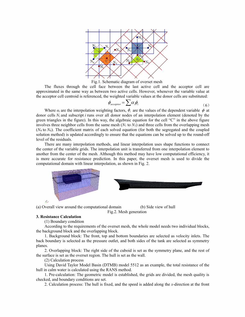
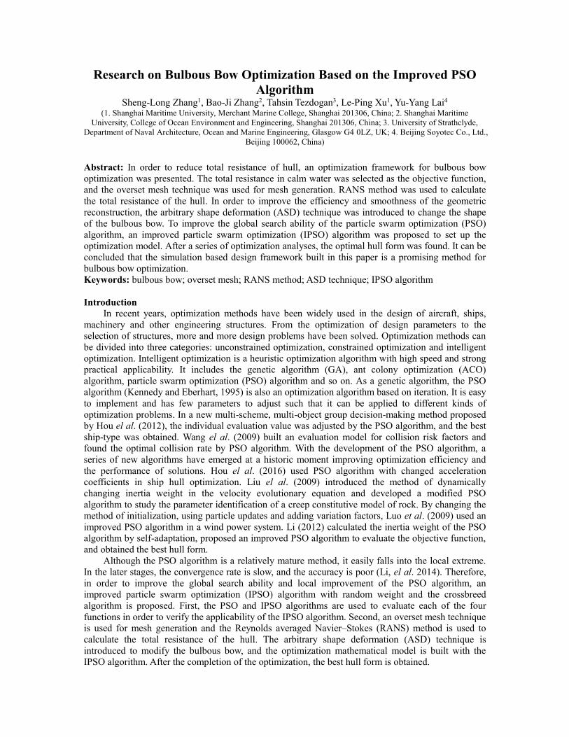
Fig.1. Schematic diagram of overset mesh

The fluxes through the cell face between the last active cell and the acceptor cell are

approximated in the same way as between two active cells. However, whenever the variable value at

the acceptor cell centroid is referenced, the weighted variable values at the donor cells are substituted:

iiacceptor （6）

Where αi are the interpolation weighting factors, are the values of the dependent variable at

donor cells Ni and subscript i runs over all donor nodes of an interpolation element (denoted by the

green triangles in the figure). In this way, the algebraic equation for the cell “C” in the above figure

involves three neighbor cells from the same mesh (N1 to N3) and three cells from the overlapping mesh

(N4 to N6). The coefficient matrix of each solved equation (for both the segregated and the coupled

solution method) is updated accordingly to ensure that the equations can be solved up to the round-off

level of the residuals.

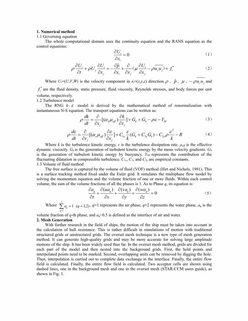
There are many interpolation methods, and linear interpolation uses shape functions to connect

the center of the variable grids. The interpolation unit is transferred from one interpolation element to

another from the center of the mesh. Although this method may have low computational efficiency, it

is more accurate for resistance prediction. In this paper, the overset mesh is used to divide the

computational domain with linear interpolation, as shown in Fig. 2.

(a) Overall view around the computational domain (b) Side view of hull

Fig.2. Mesh generation

3. Resistance Calculation

(1) Boundary condition

According to the requirements of the overset mesh, the whole model needs two individual blocks,

the background block and the overlapping block.

1. Background block: The front, top and bottom boundaries are selected as velocity inlets. The

back boundary is selected as the pressure outlet, and both sides of the tank are selected as symmetry

planes.

2. Overlapping block: The right side of the cuboid is set as the symmetry plane, and the rest of

the surface is set as the overset region. The hull is set as the wall.

(2) Calculation process

Using David Taylor Model Basin (DTMB) model 5512 as an example, the total resistance of the

hull in calm water is calculated using the RANS method.

1. Pre-calculation: The geometric model is established, the grids are divided, the mesh quality is checked, and boundary conditions are set.

2. Calculation process: The hull is fixed, and the speed is added along the x-direction at the front

i

boundary. The continuity equation (1) and the RANS equation (2) are selected as the control equations

of the whole computational domain. The RNG k– model is selected to close the equations. The

VOF method is used to simulate the free surface. The SIMPLE algorithm is selected to solve the

equations, and to start the iteration, ship speed is taken as the initial velocity. The methodology is

illustrated in Fig. 3.

Fig.3. Calculation flow of hull resistance

4. Optimization

4.1 Geometry regeneration

Based on the B-spline technique, the arbitrary shape deformation (ASD) technique is a method to

change the shape of different models using the commercial software (Sculptor). It is necessary for the

ASD volume to be set up outside the body with many control points and connections. When the

control points are moved, the shape of the relevant areas can be changed. A new surface can be created

with movements of the control points, for which third-order continuity can be maintained. This can

insure the smoothness of the new model, even under the conditions of large deformations. This direct

deformation method makes the optimization of a complex geometry possible. The specific steps are as

follows:

1. The ASD volume is built around the CAD model with different control points and connections.

The deformation volume can be finer or coarser, depending on the desired control of shape change.

2. Control points are changed by the movements of the positions and directions.

3. The new model is created according to the model generation algorithm with modified control

points.

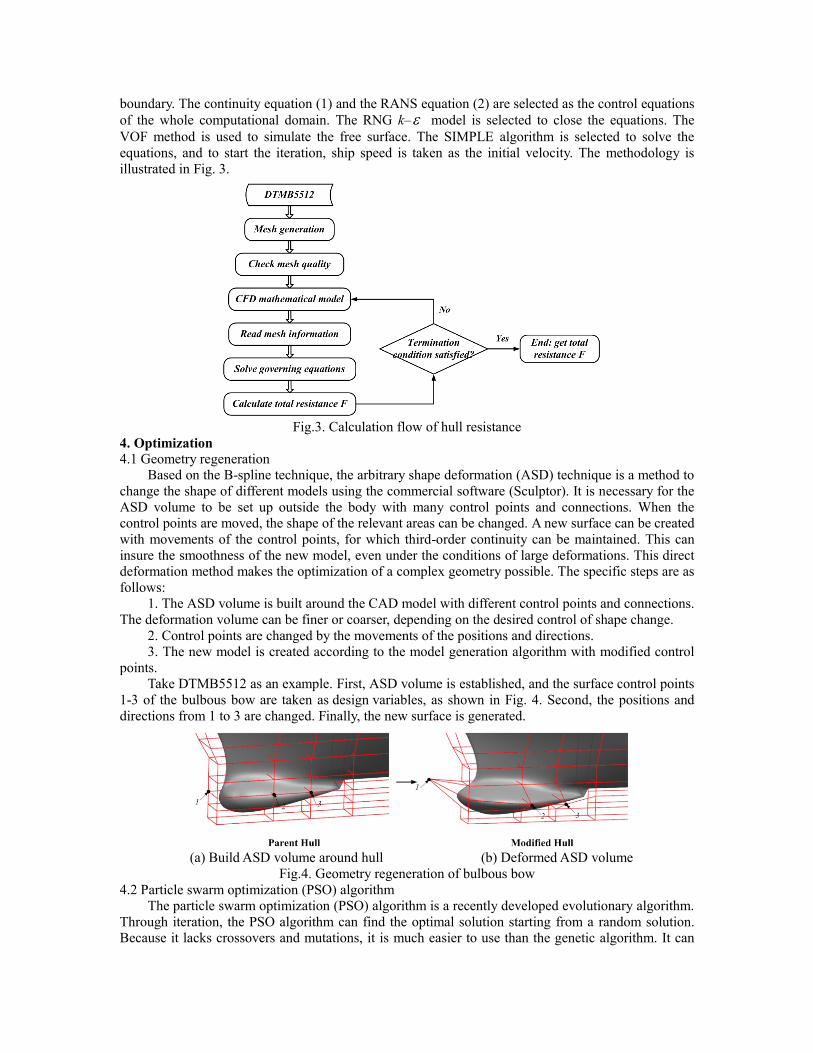
Take DTMB5512 as an example. First, ASD volume is established, and the surface control points

1-3 of the bulbous bow are taken as design variables, as shown in Fig. 4. Second, the positions and

directions from 1 to 3 are changed. Finally, the new surface is generated.

(a) Build ASD volume around hull (b) Deformed ASD volume

Fig.4. Geometry regeneration of bulbous bow

4.2 Particle swarm optimization (PSO) algorithm

The particle swarm optimization (PSO) algorithm is a recently developed evolutionary algorithm.

Through iteration, the PSO algorithm can find the optimal solution starting from a random solution.

Because it lacks crossovers and mutations, it is much easier to use than the genetic algorithm. It can

find the global optimal solution following the optimal value of the current result and evaluate the

quality of the solution by fitness. It also has a strong processing capability and good robustness.

In D-dimensional space, the i-th particle’s velocity and position can be written as Vi=(vi,1 vi,2

vi,3…vi,d) and Xi=(xi,1 xi,2 xi,3…xi,d), respectively. pbest denotes the local best solution, and gbest denotes the global optimal solution. In each iteration, the particle updates itself by tracking pbest and

gbest. After finding these two optimal values, the velocity and position of each particle is updated

according to the following formula:

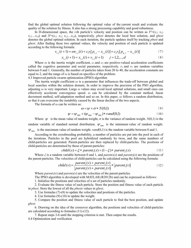
)]([)]([)()1( ,,22,,11,, txprctxprctvtv jijgjijijiji （7）

djtvtxtx jijiji ,...,2,1)1()()1( ,,, （8）

Where ω is the inertia weight coefficient, c1 and c2 are positive-valued acceleration coefficients

called the cognitive parameter and social parameter, respectively. r1 and r2 are random variables

between 0 and 1. Generally, the number of particles takes from 20 to 40, the acceleration constants are

equal to 2, and the range of ω is based on specifics of the problem.

4.3 Improved particle swarm optimization (IPSO) algorithm

The inertia weight coefficient ω is a parameter that influences the trade-off between global and

local searches within the solution domain. In order to improve the precision of the PSO algorithm,

adjusting ω is very important. Large ω values may avoid local optimal solutions, and small ones can

effectively accelerate convergence speed. ω can be calculated by the constant method, linear

decrement method, self-adaptation method and so on. In this paper, ω follows a random distribution,

so that it can overcome the instability caused by the linear decline of the two aspects.

The formula of ω can be written as:

)1,0(N （9）

)1,0()( minmaxmin rand （10）

Where is the mean value of random weight, 𝜎 is the variance of random weight. N(0,1) is the

random variable of standard normal distribution. min is the minimum value of random weight.

max is the maximum value of random weight. rand(0,1) is the random variable between 0 and 1.

According to the crossbreeding probability, a number of particles are put into the pool in each of

the iterations. Particles in the pool are hybridized randomly by twos, and the same numbers of

child-particles are generated. Parent-particles are then replaced by child-particles. The positions of

child-particles are determined by those of parent-particles:

)()1()()( 21 xparentxparentxchild （11）

Where ξ is a random variable between 0 and 1, and parent1(x) and parent2(x) are the positions of

the parent-particles. The velocities of child-particles can be calculated using the following formula:

)()()(

)()()( 1

21

21 vparentvparentvparent

vparentvparentvchild

（12）

Where parent1(v) and parent2(v) are the velocities of the parent-particles.

The IPSO algorithm is developed with MATLAB (R2012b) and can be expressed as follows:

1. Initialize the positions and velocities of a set of particles randomly.

2. Evaluate the fitness value of each particle. Store the position and fitness value of each particle

in pbest. Store the lowest of all the pbests values in gbest.

3. Use formulas (7)-(8) to update the velocities and positions of the particles.

4. Use formulas (9)-(10) to update the weight.

5. Compare the position and fitness value of each particle to find the best position, and update

gbest.

6. Drawing on the idea of the crossover algorithm, the positions and velocities of child-particles

are calculated according to formulas (11)-(12).

7. Repeat steps 3-6 until the stopping criterion is met. Then output the results. 4.4 Optimization and verification

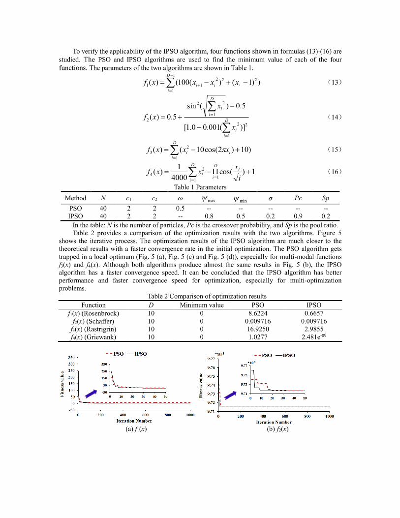
To verify the applicability of the IPSO algorithm, four functions shown in formulas (13)-(16) are

studied. The PSO and IPSO algorithms are used to find the minimum value of each of the four

functions. The parameters of the two algorithms are shown in Table 1.

1

1

222

11 ))1()(100()(D

i

ii ixxxxf （13）

2

1

2

1

22

2

)](001.00.1[

5.0)(sin

5.0)(

D

i

i

D

i

i

x

x

xf （14）

D

i

ii xxxf1

2

3 )10)2cos(10()( （15）

1)cos(4000

1)(

11

2

4

i

xxxf i

D

i

D

i

i （16）

Table 1 Parameters

Method N c1 c2 ω max min 𝜎 Pc Sp

PSO 40 2 2 0.5 -- -- -- -- --

IPSO 40 2 2 -- 0.8 0.5 0.2 0.9 0.2

In the table: N is the number of particles, Pc is the crossover probability, and Sp is the pool ratio.

Table 2 provides a comparison of the optimization results with the two algorithms. Figure 5

shows the iterative process. The optimization results of the IPSO algorithm are much closer to the

theoretical results with a faster convergence rate in the initial optimization. The PSO algorithm gets

trapped in a local optimum (Fig. 5 (a), Fig. 5 (c) and Fig. 5 (d)), especially for multi-modal functions

f3(x) and f4(x). Although both algorithms produce almost the same results in Fig. 5 (b), the IPSO

algorithm has a faster convergence speed. It can be concluded that the IPSO algorithm has better

performance and faster convergence speed for optimization, especially for multi-optimization

problems.

Table 2 Comparison of optimization results

Function D Minimum value PSO IPSO

f1(x) (Rosenbrock) 10 0 8.6224 0.6657

f2(x) (Schaffer) 10 0 0.009716 0.009716

f3(x) (Rastrigrin) 10 0 16.9250 2.9855

f4(x) (Griewank) 10 0 1.0277 2.481e-09

(a) f1(x) (b) f2(x)

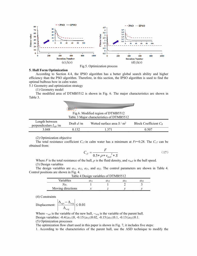
(c) f3(x) (d) f4(x)

Fig.5. Optimization process

5. Hull Form Optimization According to Section 4.4, the IPSO algorithm has a better global search ability and higher

efficiency than the PSO algorithm. Therefore, in this section, the IPSO algorithm is used to find the

optimal bulbous bow in calm water.

5.1 Geometry and optimization strategy

(1) Geometry model

The modified area of DTMB5512 is shown in Fig. 6. The major characteristics are shown in

Table 3.

Fig.6. Modified region of DTMB5512

Table 3 Major characteristics of DTMB5512

Length between

perpendiculars Lpp /m Draft d /m Wetted surface area S / m2 Block Coefficient CB

3.048 0.132 1.371 0.507

(2) Optimization objective

The total resistance coefficient CcT in calm water has a minimum at Fr=0.28. The CcT can be

obtained from:

Sv

FC

hull

cT

2

5.0 （17）

Where F is the total resistance of the hull, ρ is the fluid density, and vhull is the hull speed.

(3) Design variables

The design variables are a11, a12, a21, and a22. The control parameters are shown in Table 4.

Control positions are shown in Fig. 4.

Table 4 Design variables of DTMB5512

Variables a11 a12 a21 a22 No. 1 1 2 3

Moving directions x z y y

(4) Constraints

Displacement: 01.0

org

orgopt

Where --opt is the variable of the new hull, --org is the variable of the parent hull.

Design variables: -0.4≤a11≤0, -0.15≤a12≤0.02, -0.15≤a21≤0.1, -0.13≤a22≤0.1.

(5) Optimization processes

The optimization flow chart used in this paper is shown in Fig. 7, it includes five steps:

1. According to the characteristics of the parent hull, use the ASD technique to modify the

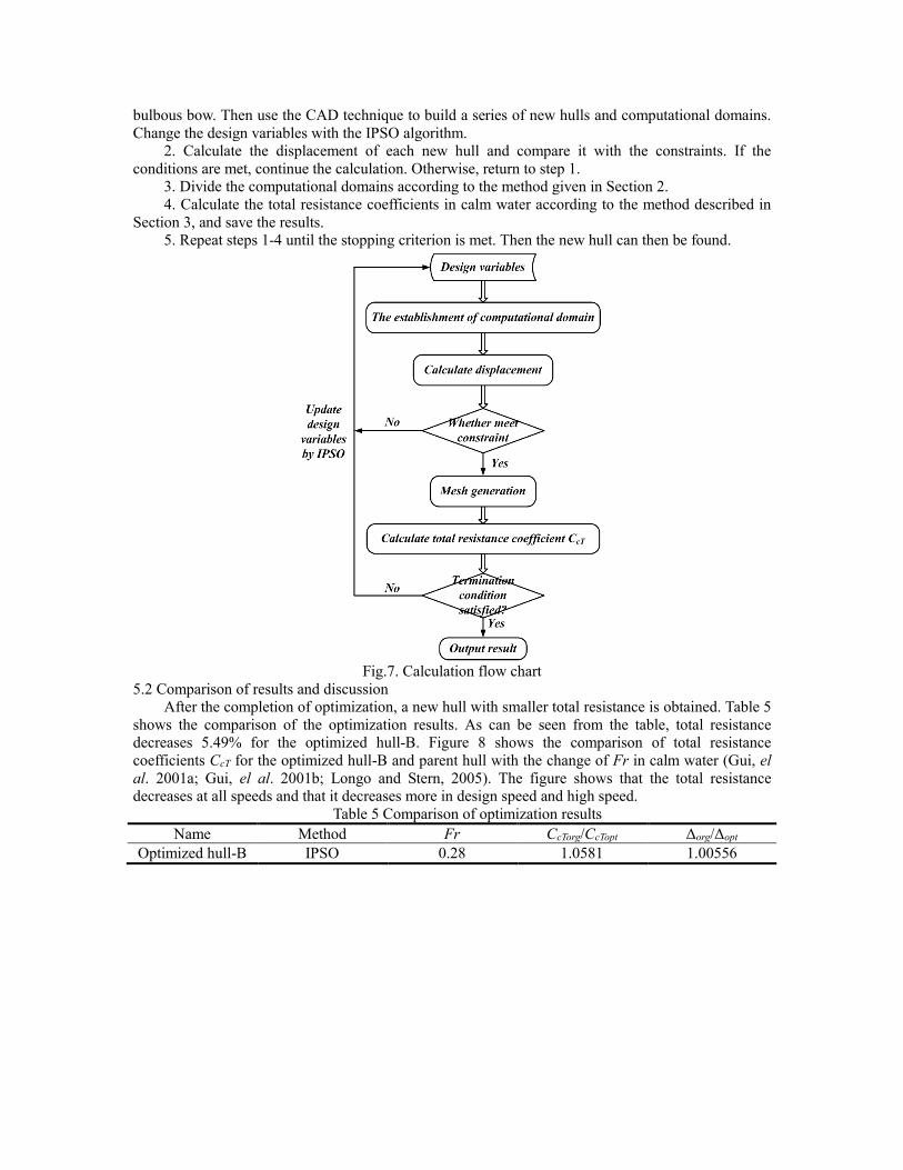
bulbous bow. Then use the CAD technique to build a series of new hulls and computational domains.

Change the design variables with the IPSO algorithm.

2. Calculate the displacement of each new hull and compare it with the constraints. If the

conditions are met, continue the calculation. Otherwise, return to step 1.

3. Divide the computational domains according to the method given in Section 2.

4. Calculate the total resistance coefficients in calm water according to the method described in

Section 3, and save the results.

5. Repeat steps 1-4 until the stopping criterion is met. Then the new hull can then be found.

Fig.7. Calculation flow chart

5.2 Comparison of results and discussion

After the completion of optimization, a new hull with smaller total resistance is obtained. Table 5

shows the comparison of the optimization results. As can be seen from the table, total resistance

decreases 5.49% for the optimized hull-B. Figure 8 shows the comparison of total resistance

coefficients CcT for the optimized hull-B and parent hull with the change of Fr in calm water (Gui, el

al. 2001a; Gui, el al. 2001b; Longo and Stern, 2005). The figure shows that the total resistance

decreases at all speeds and that it decreases more in design speed and high speed.

Table 5 Comparison of optimization results

Name Method Fr CcTorg/CcTopt Δorg/Δopt

Optimized hull-B IPSO 0.28 1.0581 1.00556

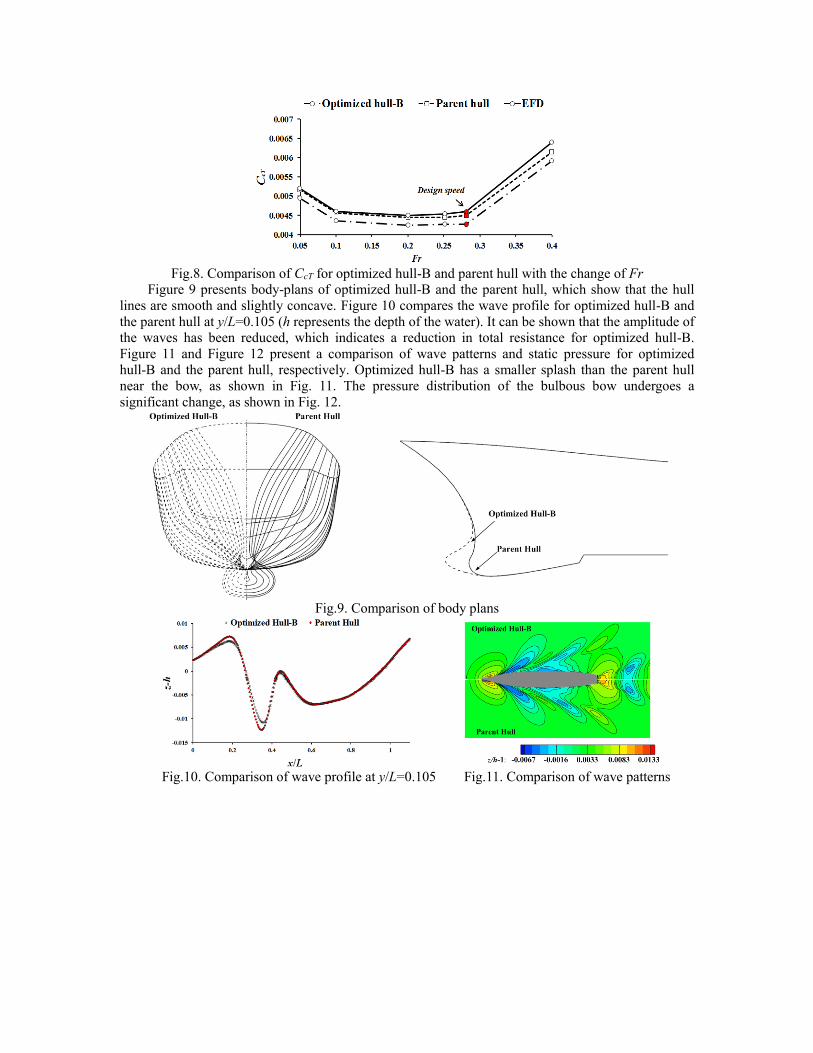
Fig.8. Comparison of CcT for optimized hull-B and parent hull with the change of Fr

Figure 9 presents body-plans of optimized hull-B and the parent hull, which show that the hull

lines are smooth and slightly concave. Figure 10 compares the wave profile for optimized hull-B and

the parent hull at y/L=0.105 (h represents the depth of the water). It can be shown that the amplitude of

the waves has been reduced, which indicates a reduction in total resistance for optimized hull-B.

Figure 11 and Figure 12 present a comparison of wave patterns and static pressure for optimized

hull-B and the parent hull, respectively. Optimized hull-B has a smaller splash than the parent hull

near the bow, as shown in Fig. 11. The pressure distribution of the bulbous bow undergoes a

significant change, as shown in Fig. 12.

Fig.9. Comparison of body plans

Fig.10. Comparison of wave profile at y/L=0.105 Fig.11. Comparison of wave patterns

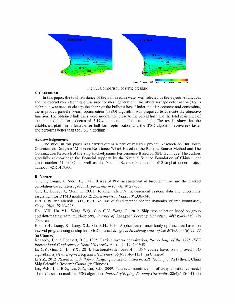
Fig.12. Comparison of static pressure

6. Conclusion

In this paper, the total resistance of the hull in calm water was selected as the objective function,

and the overset mesh technique was used for mesh generation. The arbitrary shape deformation (ASD)

technique was used to change the shape of the bulbous bow. Under the displacement and constraints,

the improved particle swarm optimization (IPSO) algorithm was proposed to evaluate the objective

function. The obtained hull lines were smooth and close to the parent hull, and the total resistance of

the obtained hull form decreased 5.49% compared to the parent hull. The results show that the

established platform is feasible for hull form optimization and the IPSO algorithm converges faster

and performs better than the PSO algorithm.

Acknowledgements

The study in this paper was carried out as a part of research project: Research on Hull Form

Optimization Design of Minimum Resistance Which Based on the Rankine Source Method and The

Optimization Research of the Ship Hydrodynamic Performance Based on SBD technique. The authors

gratefully acknowledge the financial supports by the National Science Foundation of China under

grant number 51009087, as well as the National Science Foundation of Shanghai under project

number 14ZR1419500.

Reference

Gui, L., Longo, J., Stern, F., 2001. Biases of PIV measurement of turbulent flow and the masked

correlation-based interrogation, Experiments in Fluids, 30:27~35.

Gui, L., Longo, J., Stern, F., 2001. Towing tank PIV measurement system, data and uncertainty

assessment for DTMB model 5512, Experiments in Fluids, 31:336~346.

Hirt, C.W. and Nichols, B.D., 1981. Volume of fluid method for the dynamics of free boundaries,

Comp. Phys, 39:20~225.

Hou, Y.H., Hu, Y.L., Wang, W.Q., Guo, C.Y., Wang, C., 2012. Ship type selection based on group

decision-making with multi-objects, Journal of Shanghai Jiaotong University, 46(3):385~389. (in

Chinese)

Hou, Y.H., Liang, X., Jiang, X.J., Shi, X.H., 2016. Application of uncertainty optimization based on

interval programming in ship hull SBD optimal design, J. Huazhong Univ. of Sic.&Tech., 44(6):72~77.

(in Chinese)

Kennedy, J. and Eberhart, R.C., 1995. Particle swarm optimization, Proceedings of the 1995 IEEE

International Conferenceon Neural Networks, Australia, 1942~1948.

Li, G.Y., Guo, C., Li, Y.X., 2014. Fractional-order control of USV course based on improved PSO

algorithm, Systems Engineering and Electronics, 36(6):1146~1151. (in Chinese)

Li S.Z., 2012. Research on hull form design optimization based on SBD technique, Ph.D thesis, China

Ship Scientific Research Center. (in Chinese)

Liu, W.B., Liu, B.G., Liu, Z.Z., Cui, S.D., 2009. Parameter identification of creep constitutive model

of rock based on modified PSO algorithm, Journal of Beijing Jiaotong University, 33(4):140~143. (in

Chinese)

Longo, J. and Stern, F., 2005. Uncertainty assessment for towing tank tests with example for surface

combatant DTMB model 5415, J. Ship Research, 49(1):55~68.

Luo, J., Wu, Z.Q., Leng, G.F., Cui, S.D., 2009. VAR optimization in wind power system based on

improved PSO, Insulating Material, 42(2):67~70. (in Chinese)

STAR-CCM users guide.

Wang, D.Y., Liu, Y., Xia, L.J., 2009. Studies on turning angle to avoid collision between ships with

PSO arithmetic, Computer Engineering and Design, 30(14):3380~3382. (in Chinese)