Research methodology unit6

RESEARCH METHODOLOGY – UNIT 6Data Reduction and Analysis

CONTENTS

Meaning and Importance of Data Reduction

Data Reduction Process

Selected Techniques of Data Analysis

2

Rese

arc

h M

eth

od

olo

gy -

Unit 6

PROCESSING AND ANALYSIS OF DATA

The data, after collection, has to be processed and

analyzed in accordance with the outline laid down for

the purpose at the time of developing the research plan.

This is essential for a scientific study and for ensuring

that we have all relevant data for making contemplated

comparisons and analysis.

Technically speaking, processing implies editing, coding,

classification and tabulation of collected data so that

they are amenable to analysis.

The term analysis refers to the computation of certain

measures along with searching for patterns of

relationship that exist among data groups.3

Rese

arc

h M

eth

od

olo

gy -

Unit 6

PROCESSING AND ANALYSIS OF DATA

Thus, “in the process of analysis, relationships or

differences supporting or conflicting with original or

new hypotheses should be subjected to statistical

tests of significance to determine with what validity

data can be said to indicate and conclusions”.

4

Rese

arc

h M

eth

od

olo

gy -

Unit 6

PROCESSING OPERATIONS

Editing is the process of examining the collected

raw data (especially in surveys) to detect errors and

omissions and to correct these when possible.

Furthermore, it involves a careful scrutiny of the

completed questionnaires and/or schedules.

Editing is done to assure that the data are accurate,

consistent with other facts gathered, uniformly

entered, as complete as possible and have been

well arranged to facilitate coding and tabulation.

5

Rese

arc

h M

eth

od

olo

gy -

Unit 6


Field editing consists in the review of the reporting

forms by the investigator for completing (translating

or rewriting) what the latter has written in

abbreviated and/or illegible form at the time of

recording the respondents’ responses.

Central editing should take place when all forms or

schedules have been completed and returned to

the office. This type of editing implies that all forms

should get a thorough editing by a single editor in a

small study and by a team of editors in case of a

large inquiry.

6

Rese

arc

h M

eth

od

olo

gy -

Unit 6


Coding refers to the process of assigning numeralsor other symbols to answers so that responses canbe put into a limited number of categories orclasses.

Such classes should be appropriate to the researchproblem under consideration and must possess thecharacteristic of exhaustiveness (i.e., there must bea class for every data item) and also that of mutualexclusivity which means that a specific answer canbe placed in one and only cell in a given categoryset.

Another rule to be observed is that ofunidimensionality by which is meant that everyclass is defined in terms of only one concept.

7

Rese

arc

h M

eth

od

olo

gy -

Unit 6


Coding is necessary for efficient analysis and

through it the several replies may be reduced to a

small number of classes which contain the critical

information required for the analysis.

Coding decisions should be usually be taken at the

designing stage of the questionnaire which makes it

possible to precode the questionnaire choices thus

making it faster for computer tabulation later on.

Coding errors should be altogether eliminated or

reduced to the minimum level.

8

Rese

arc

h M

eth

od

olo

gy -

Unit 6


Classification

Most research studies result in a large volume of raw

data which must be reduced into homogeneous groups

if we are to get meaningful relationships.

Classification of data happens to be the process of

arranging data in groups or classes on the basis of

common characteristics.

Can be one of the following two types, depending upon

the nature of the phenomenon involved:

Classification according to attributes

Classification according to class intervals

9

Rese

arc

h M

eth

od

olo

gy -

Unit 6

CLASSIFICATION ACCORDING TO ATTRIBUTES

Data are classified on the basis of common

characteristics which can either be descriptive

(such as literacy, sex, honesty, etc.) or numerical

(such as weight, height, income etc.).

Descriptive characteristics refer to qualitative

phenomenon which cannot be measured

quantitatively; only their presence or absence in an

individual item can be noticed.

Data obtained in this way on the basis of certain

attributes are known as statistics of attributes and

their classification is said to be classification

according to attributes. 10

Rese

arc

h M

eth

od

olo

gy -

Unit 6

CLASSIFICATION ACCORDING TO ATTRIBUTES

Such a classification can be simple classification

or manifold classification.

In simple classification, we consider only one

attribute and divide the universe into two classes –

one class consisting of items possessing the given

attribute and the other class consisting of items

which do not possess the given attribute.

In manifold classification, we consider two or more

attributes simultaneously, and divide the data into a

number of classes. Total number of classes of final

order is given by 2^n, where n = number of

attributes considered.) 11

Rese

arc

h M

eth

od

olo

gy -

Unit 6

CLASSIFICATION ACCORDING TO CLASS-

INTERVALS

Unlike descriptive characteristics, the numerical characteristics refer to quantitative phenomenon which can be measured through some statistical units.

Data relating to income, production, age, weight etc. come under this category.

Such data are known as statistics of variables and are classified on the basis of class intervals.

For instance, persons whose income, say, are within Rs. 201 to Rs. 400 can form one group, those whose incomes are within Rs. 401 to Rs. 600 can form another group and so on.

Each group or class-interval, thus, has an upper limit as well as a lower limit which are known as class limits.

The difference between the two class limits is known as class magnitude.

The number of items which fall in a given class is known as the frequency of the given class.

12

Rese

arc

h M

eth

od

olo

gy -

Unit 6


INTERVALS

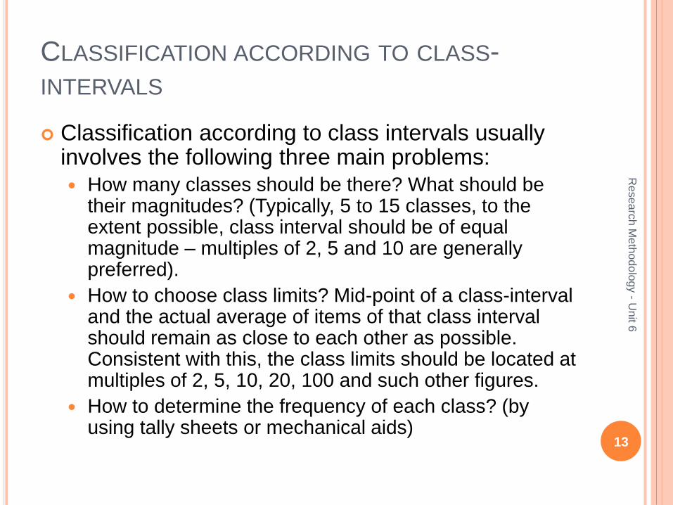
Classification according to class intervals usually involves the following three main problems:

How many classes should be there? What should be their magnitudes? (Typically, 5 to 15 classes, to the extent possible, class interval should be of equal magnitude – multiples of 2, 5 and 10 are generally preferred).

How to choose class limits? Mid-point of a class-interval and the actual average of items of that class interval should remain as close to each other as possible. Consistent with this, the class limits should be located at multiples of 2, 5, 10, 20, 100 and such other figures.

How to determine the frequency of each class? (by using tally sheets or mechanical aids)

13

Rese

arc

h M

eth

od

olo

gy -

Unit 6


INTERVALS

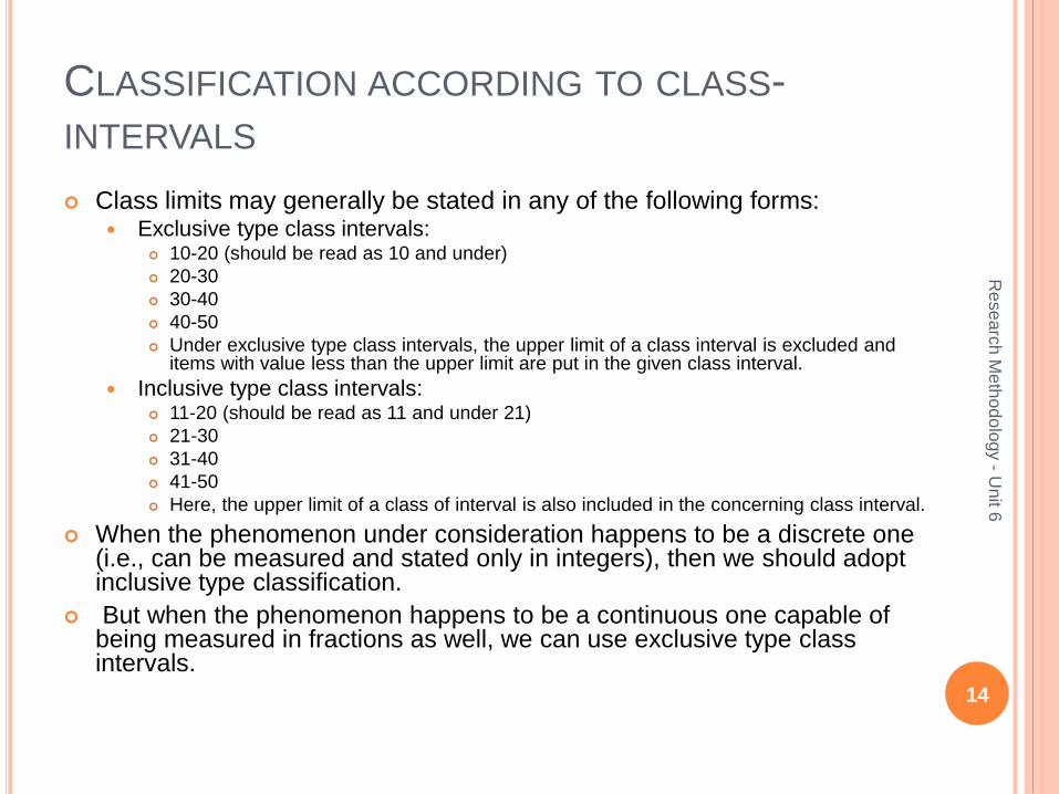
Class limits may generally be stated in any of the following forms: Exclusive type class intervals:

10-20 (should be read as 10 and under)

20-30

30-40

40-50

Under exclusive type class intervals, the upper limit of a class interval is excluded and items with value less than the upper limit are put in the given class interval.

Inclusive type class intervals: 11-20 (should be read as 11 and under 21)

21-30

31-40

41-50

Here, the upper limit of a class of interval is also included in the concerning class interval.

When the phenomenon under consideration happens to be a discrete one (i.e., can be measured and stated only in integers), then we should adopt inclusive type classification.

But when the phenomenon happens to be a continuous one capable of being measured in fractions as well, we can use exclusive type class intervals.

14

Rese

arc

h M

eth

od

olo

gy -

Unit 6

TABULATION

When a mass of data has been assembled, it

becomes necessary for the researcher to arrange

the same in some kind of concise and logical order.

This procedure is known as tabulation.

Thus, tabulation is the process of summarizing raw

data and displaying the same in compact form (i.e.,

in the form of statistical tables) for further analysis.

In a broader sense, tabulation is an orderly

arrangement of data in columns and rows.

15

Rese

arc

h M

eth

od

olo

gy -

Unit 6

TABULATION

Tabulation can be done by hand or by mechanical

or electronic devices.

The choice depends on the size and type of study,

cost considerations, time pressures and the

availability of tabulating machines or computers.

Mechanical or electronic tabulation – in relatively

large queries, hand tabulation in case of small

queries, where the number of questionnaires is

small and they are of relatively short length.

16

Rese

arc

h M

eth

od

olo

gy -

Unit 6

TABULATION

Tabulation may be classified as simple and complex tabulation.

Simple tabulation gives information about one or more groups of independent questions, whereas complex tabulation shows the division of data into two or more categories and as such is designed to give information concerning one or more sets of inter-related questions.

Simple tabulation generally results in one-way tables which supply answers to questions about one characteristic of data only.

Complex tabulation usually results in two-way tables (which give information about two interrelated characteristics of data), three-way tables (giving information about three interrelated characteristics of data) or still higher ordered tables, also known as manifold tables, which supply information about several interrelated characteristics of data.

Two-way, three-way and manifold tables are all examples of what is sometimes described as cross-tabulation.

17

Rese

arc

h M

eth

od

olo

gy -

Unit 6

SOME PROBLEMS IN PROCESSING

The problem concerning “Don’t know” (or DK)

responses.

Use of percentages

18

Rese

arc

h M

eth

od

olo

gy -

Unit 6

ELEMENTS/TYPES OF ANALYSIS

Analysis, particularly in case of survey or experimental data, involves estimating the values of unknown parameters of the population and testing of hypotheses for drawing inferences.

Analysis may, therefore, be categorized as descriptive analysis and inferential analysis.

Descriptive analysis is largely the study of distributions of one variable.

This study provides us with the profiles of companies, work groups, persons and other subjects on any multitude of characteristics such as size, composition, efficiency, preferences etc.

This sort of analysis may be in respect of one variable (unidimensional analysis), or in respect of two variables (bivariate analysis) or in respect of more than two variables (multivariate analysis). 19

Rese

arc

h M

eth

od

olo

gy -

Unit 6


Correlation analysis studies the joint variation of two or more variables for determining the amount of correlation between two or more variables.

Causal analysis is concerned with the study of how one or more variables affect changes in another variable. It is thus a study of functional relationships existing between two or more variables. This analysis can be termed as regression analysis.

Causal analysis is considered relatively more important in experimental researches, whereas in most social and business researches, our interest lies in understanding and controlling relationships between variables then with determining causes per se and as such we consider correlation analysis as relatively more important.

20

Rese

arc

h M

eth

od

olo

gy -

Unit 6


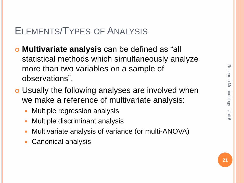
Multivariate analysis can be defined as “all

statistical methods which simultaneously analyze

more than two variables on a sample of

observations”.

Usually the following analyses are involved when

we make a reference of multivariate analysis:

Multiple regression analysis

Multiple discriminant analysis

Multivariate analysis of variance (or multi-ANOVA)

Canonical analysis

21

Rese

arc

h M

eth

od

olo

gy -

Unit 6

MULTIVARIATE ANALYSIS

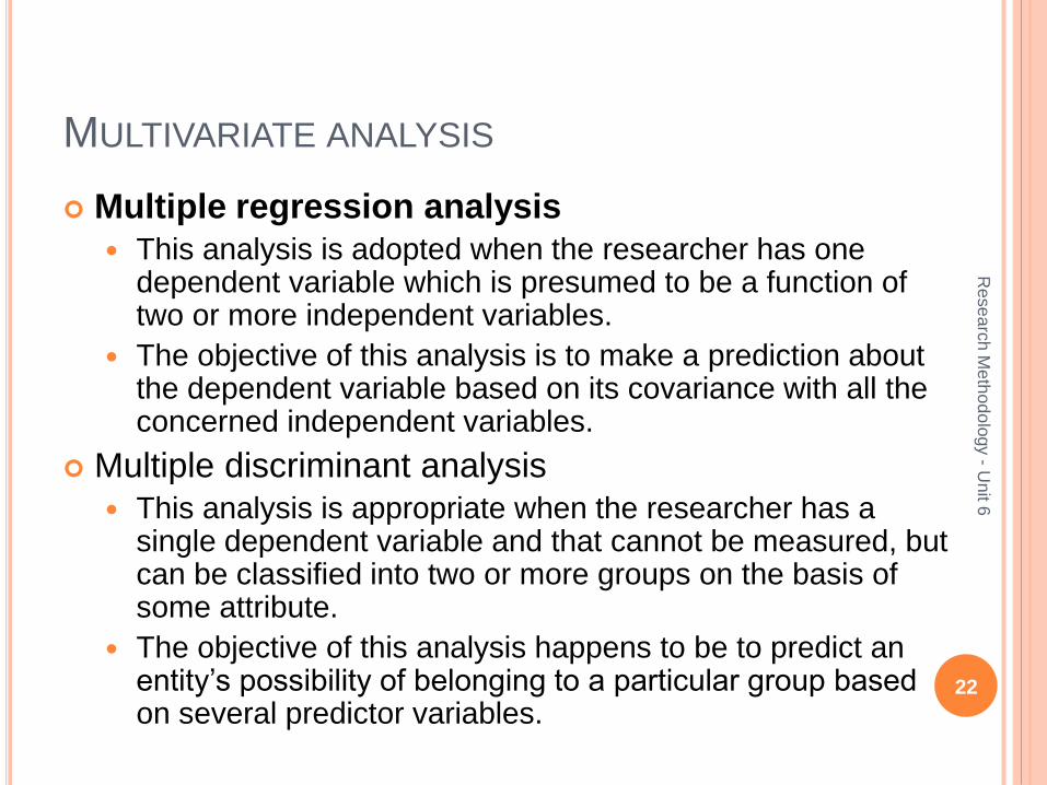
Multiple regression analysis

This analysis is adopted when the researcher has one dependent variable which is presumed to be a function of two or more independent variables.

The objective of this analysis is to make a prediction about the dependent variable based on its covariance with all the concerned independent variables.

Multiple discriminant analysis

This analysis is appropriate when the researcher has a single dependent variable and that cannot be measured, but can be classified into two or more groups on the basis of some attribute.

The objective of this analysis happens to be to predict an entity’s possibility of belonging to a particular group based on several predictor variables.

22

Rese

arc

h M

eth

od

olo

gy -

Unit 6

MULTIVARIATE ANALYSIS

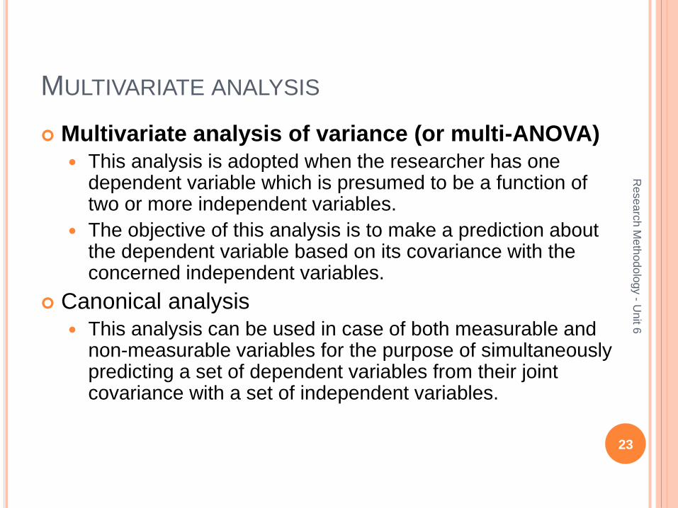
Multivariate analysis of variance (or multi-ANOVA)

This analysis is adopted when the researcher has one dependent variable which is presumed to be a function of two or more independent variables.

The objective of this analysis is to make a prediction about the dependent variable based on its covariance with the concerned independent variables.

Canonical analysis

This analysis can be used in case of both measurable and non-measurable variables for the purpose of simultaneously predicting a set of dependent variables from their joint covariance with a set of independent variables.

23

Rese

arc

h M

eth

od

olo

gy -

Unit 6

INFERENTIAL ANALYSIS

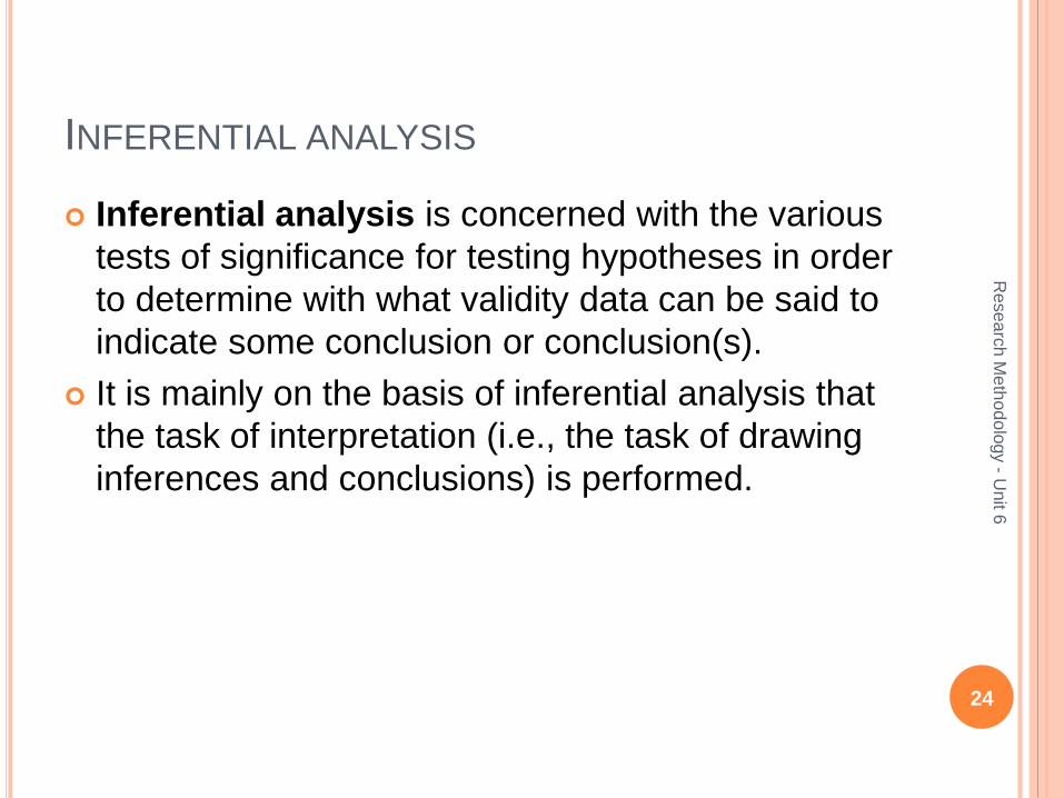
Inferential analysis is concerned with the various

tests of significance for testing hypotheses in order

to determine with what validity data can be said to

indicate some conclusion or conclusion(s).

It is mainly on the basis of inferential analysis that

the task of interpretation (i.e., the task of drawing

inferences and conclusions) is performed.

24

Rese

arc

h M

eth

od

olo

gy -

Unit 6

STATISTICS IN RESEARCH

There are two major areas of statistics viz.,

descriptive statistics and inferential statistics.

Descriptive statistics concern the development of

certain indices from the raw data, whereas inferential

statistics concern with the process of generalization.

Inferential statistics are also known as sampling

statistics and are mainly concerned with two major

type of problems:

the estimation of population parameters

the testing of statistical hypotheses

25

Rese

arc

h M

eth

od

olo

gy -

Unit 6


The important statistical measures that are used to summarize the survey/research data are:

Measures of central tendency or statistical averages arithmetic average or mean, median and mode, geometric mean

and harmonic mean

Measures of dispersion Variance and its square root – the standard deviation, range etc.

For comparison purposes, mostly the coefficient of standard deviation or the coefficient of variation.

Measures of asymmetry (skewness) Measure of skewness and kurtosis are based on mean and mode

or on mean and median.

Other measures of skewness, based on quartiles or on the methods of moments, are also used sometimes. Kurtosis is also used to measure the peakedness of the curve of frequency distribution.

26

Rese

arc

h M

eth

od

olo

gy -

Unit 6


Measures of relationship

Karl Pearson’s coefficient of correlation is the frequently used

measure in case of statistics of variables.

Yule’s coefficient of association is used in case of statistics of

attributes.

Multiple correlation coefficient, partial correlation coefficient,

regression analysis etc., are other important measures.

Other measures

Index numbers, analysis of time series, coefficient of contingency,

etc., are other measures that may as well be used depending

upon the nature of the problem under study.

27

Rese

arc

h M

eth

od

olo

gy -

Unit 6

MEASURES OF CENTRAL TENDENCY

Measures of central tendency (or statistical averages)

tell us the point about which items have a tendency to

cluster.

Such a measure is considered as the most

representative figure for the entire mass of data.

Mean, median and mode are the most popular

averages.

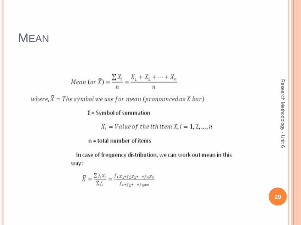
Mean, also known as arithmetic average, is the most

common measure of central tendency and may be

defined as the value which we get dividing the total of

the values of various given items in a series by the

total number of items. 28

Rese

arc

h M

eth

od

olo

gy -

Unit 6

MEAN

29

Rese

arc

h M

eth

od

olo

gy -

Unit 6

MEAN

30

Rese

arc

h M

eth

od

olo

gy -

Unit 6

MEAN

Mean is the simplest measure of central tendency and is a widely used measure.

Its chief use consists in summarizing the essential features of a series and in enabling data to be compared.

It is amenable to algebraic treatment and is used in further statistical calculations.

It is a relatively stable measure of central tendency.

But it suffers from some limitations viz., it is unduly affected by extreme items; it may not coincide with the actual value if an item in series, and it may lead to wrong impressions, particularly when the item values are not given in the average.

However, mean is better than other averages, specially in economic and social studies where direct quantitative measurements are possible.

31

Rese

arc

h M

eth

od

olo

gy -

Unit 6

MEDIAN

Median is the value of the middle item of series when it is arranged in ascending or descending order of magnitude.

It divides the series into two halves: in one half all items are less than the median, whereas in the other half all items have values higher than the median,

If the values of the items arranged in ascending order are: 60, 74, 80, 88, 90, 95, 100, then the value of the 4’th item viz., 88 is the value of the median.

We can also write as: Median(M) = Value of ((n+1)/2)th item. 32

Rese

arc

h M

eth

od

olo

gy -

Unit 6

MEDIAN

Median is a positional average and is used only in

the context of qualitative phenomena, for example,

in estimating intelligence etc., which are often

encountered in sociological fields.

Median is not useful where items need to be

assigned relative importance and weights.

It is not frequently used in sampling statistics.

33

Rese

arc

h M

eth

od

olo

gy -

Unit 6

MODE

Mode is the most commonly or frequently occurring value in the series.

The mode in a distribution is that item around which there is maximum concentration.

In general, mode is the size of the item which has the maximum frequency, but at times such an item may not be mode on account of the effect of the frequencies of the neighboring items.

Like median, mode is a positional average and is not affected by the value of the extreme items.

It is therefore, useful in all situations where we want to eliminate the effect of extreme variations.

Mode is particularly useful in the study of popular sizes, for example, size of the shoe most in demand.

However, mode is not amenable to algebraic treatment and sometimes remains indeterminate when we have two or more model values in a series.

It is considered unsuitable in cases where we want to give relative importance to items under consideration.

34

Rese

arc

h M

eth

od

olo

gy -

Unit 6

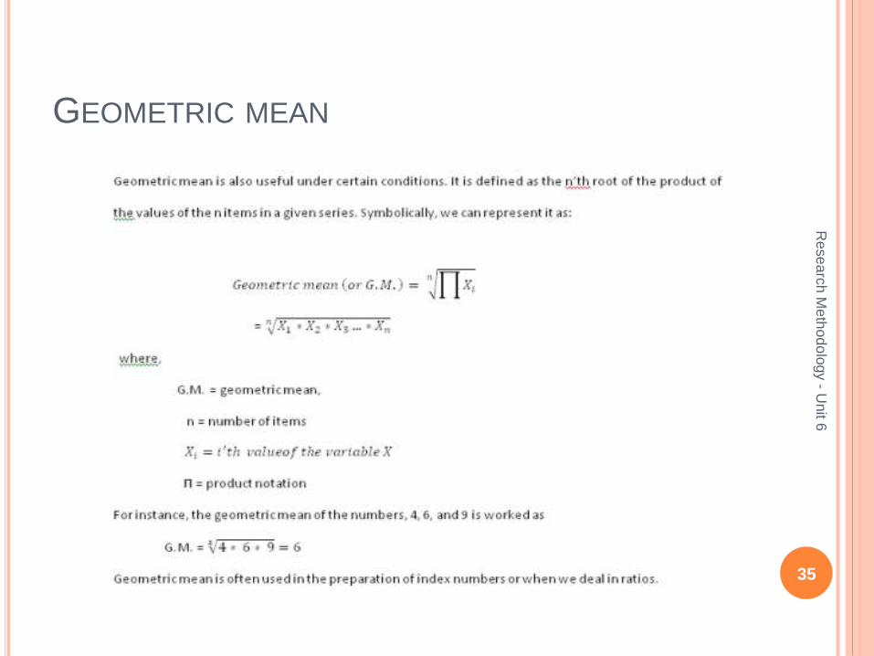
GEOMETRIC MEAN

35

Rese

arc

h M

eth

od

olo

gy -

Unit 6

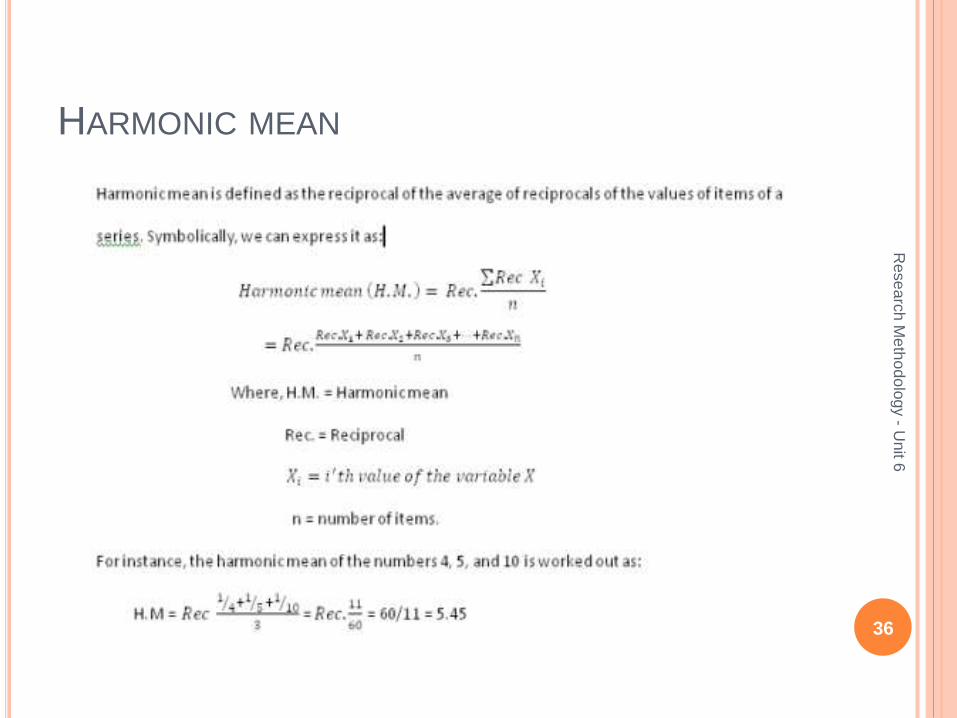
HARMONIC MEAN

36

Rese

arc

h M

eth

od

olo

gy -

Unit 6

HARMONIC MEAN

Harmonic mean is of limited application, particularly

in cases where time and rate are involved.

It gives largest weight to the smallest item and

smallest weight to the largest item.

As such, it is used in cases like time and motion

study where time is a variable and distance a

constant.

37

Rese

arc

h M

eth

od

olo

gy -

Unit 6

MEASURES OF DISPERSION

An average can represent a series only as best as

a single figure can, but it certainly cannot reveal the

entire story of any phenomenon under study.

Specially, it fails to give any idea about the scatter

of the values of items of a variable in the series

around the true value of average.

In order to measure this scatter, statistical devices

called measures of dispersion are calculated.

Important measures of dispersion are : i) range, ii)

mean deviation and iii) standard deviation.

38

Rese

arc

h M

eth

od

olo

gy -

Unit 6


Range is the simplest possible measure of dispersion and is defined as the difference between the values of the extreme items of a series.

Thus, Range = (Highest value of an item in a series) – (Lowest value of

an item in a series)

The utility of range is that it gives an idea of the variability very quickly, but the drawback is that range is affected very greatly by fluctuations of sampling.

Its value is never stable, being based on only two values of a variable.

Hence, it is used as a rough measure of variability and is not considered as an appropriate measure in serious studies. 39

Rese

arc

h M

eth

od

olo

gy -

Unit 6


Mean deviation is the average of differences of

the values of items from some average of the

series.

Such a difference is technically described as

deviation.

In calculating the deviation, we ignore the minus

sign of the deviations, while taking their total for

obtaining the mean deviation.

40

Rese

arc

h M

eth

od

olo

gy -

Unit 6


See the formulae on board.

When mean deviation is divided by the average used in finding out the mean deviation itself, the resulting quantity is described as the coefficient of mean deviation.

Coefficient of mean deviation is a relative measure of dispersion and is comparable to similar measure of other series.

Mean deviation and its coefficient are used in statistical studies for judging the variability, and thereby render the study of central tendency of a series more precise by throwing light on the typicalness of the average.

Better measurement of variability than range as it takes into consideration the values of all items of a series.

However, not a frequently used measure as it is not amenable to algebraic process.

41

Rese

arc

h M

eth

od

olo

gy -

Unit 6


Standard deviation is the most widely used measure of dispersion series and is commonly denoted by the symbol ‘σ’, pronounced as sigma.

It is defined as the square-root of the average of squares of deviation, when such deviations for the values of the individual items in a series are obtained from the arithmetic average.

See the formulae on board.

When we divide the standard deviation by arithmetic average of the series, the resulting quantity is known as coefficient of standard deviation, which happens to be the relative measure and is often used for comparing with similar measure of other series.

When this coefficient of standard deviation is multiplied by 100, the resulting figure is known as coefficient of variation.

Sometimes, the square of the standard deviation, known as variance, is frequently used in the context of analysis of variation.

42

Rese

arc

h M

eth

od

olo

gy -

Unit 6


The standard deviation (along with several other

related measures like variance, coefficient of

variation, etc.) is used mostly in research studies

and is regarded a very satisfactory measure of

dispersion in series.

It is amenable to mathematical manipulation

because the algebraic signs are not ignored in its

calculation.

It is less affected by the fluctuations in sampling.

It is popularly used in the context of estimation and

testing of hypotheses.43

Rese

arc

h M

eth

od

olo

gy -

Unit 6

MEASURES OF ASYMMETRY(SKEWNESS)

When the distribution of items in a series happens to be perfectly symmetrical, we have the following type of curve for the distribution.

See on board.

Such a curve is technically described as a normal curve and the relating distribution as normal distribution.

Such a curve is perfectly bell shaped curve in which case the value of X under bar or M or Z is just the same and skewness is altogether absent.

But if the curve is distorted on the right side, we have positive skewnesss and when the curve is distorted towards the left, we have negative skewness.

Look at the figures on board.44

Rese

arc

h M

eth

od

olo

gy -

Unit 6


Skewness, is, thus, a measure of asymmetry and shows the manner in which the items are clustered around the average.

In a symmetrical distribution, the items show a perfect balance on either side of a mode, but in a skewed distribution, the balance is thrown to one side.

The amount by which the balance exceeds on one side measures the skewness of the series.

The difference between the mean, median and mode provides an easy way expressing skewness in a series.

In case of positive skewness, we have Z< M<X under bar and in case of negative skewness, we have X under bar < M < Z.

Look for the formulae on the board about how the skewness is measured. 45

Rese

arc

h M

eth

od

olo

gy -

Unit 6


The significance of the skewness lies in the fact that through it one can study the formation of a series and can have the idea about the shape of the curve, whether normal or otherwise, when the items of a given series are plotted on a graph.

Kurtosis is the measure of flat-toppedness of a curve.

A bell shaped curve or the normal curve is Mesokurtic because it is kurtic in the centre; but if the curve is relatively more peaked than the normal curve, it is Leptokurtic.

Similarly, if a curve is more flat than the normal curve, it is called Platykurtic.

In brief, kurtosis is the humpedness of the curve and points to the nature of the distribution of items in the middle of a series.

Knowing the shape of the distribution curve is crucial to the use of statistical methods in research analysis since most methods make specific assumptions about the nature of the distribution curve.

46

Rese

arc

h M

eth

od

olo

gy -

Unit 6

MEASURES OF RELATIONSHIP

In case of bivariate and multi-variate populations, we often wish to know the relation of the two and/or more variables in the data to one another.

We may like to know, for example, whether the number of hours students devote for studies is somehow related to their family income, to age, to sex or to similar other factor.

We need to answer the following two types of questions in bivariate and\or multivariate populations: Does there exist association or correlation between the two

(or more) variables? If yes, of what degree?

Is there any cause and effect relationship between the two variables in case of bivariate population or between one variable on one side and two or more variables on the other side in case of multivariate population? If yes, of what degree and in which direction?

47

Rese

arc

h M

eth

od

olo

gy -

Unit 6


The first question is answered by the use of the correlation technique and the second question by the technique of regression.

There are several methods of applying the two techniques, but the important ones are as under: In case of bivariate population:

Correlation can be studied through a) cross tabulation, b) Charles Spearman’s coefficient of correlation, c) Karl Pearson’s coefficient correlation.

Cause and effect relationship can be studied through simple regression equations.

In case of multivariate population:

Correlation can be studied through a) coefficient of multiple correlation, b) coefficient of partial correlation.

Cause and effect relationship can be studied through multiple regression equations. 48

Rese

arc

h M

eth

od

olo

gy -

Unit 6


Cross tabulation approach Cross tabulation approach is specially useful when the data are in nominal

form.

Under it, we classify the variables in these sub-categories.

Then, we look for interactions between them which may be symmetrical, reciprocal or asymmetrical.

A symmetrical relationship is one in which the two variables vary together, but we assume that neither variable is due to the other.

A reciprocal relationship exists when the two variables mutually influence or reinforce each other.

A symmetrical relationship is said to exist if one variable (the independent variable) is responsible for another variable (the dependent variable).

The cross classification procedure begins with a two-way table, which indicates whether there is or there is not an interrelationship between the two variables.

This sort of analysis can be further elaborated in which case a third factor is introduced into the association through cross-classifying the variables.

By doing so, we find conditional relationships in which factor X appears to affect factor Y only when factor Z is held constant.

The correlation, if any found through this approach, is not considered a very powerful form of statistical correlation and accordingly we use some other methods when data happen to be either ordinal or interval or ratio data.

49

Rese

arc

h M

eth

od

olo

gy -

Unit 6


Charles Spearman’s coefficient of correlation (or rank correlation) This is the technique of determining the degree of correlation between

two variables in case of ordinal data where ranks are given to the different values of the variables.

The main objective of this coefficient is to determine the extent to which the two sets of ranking are similar or dissimilar.

Look for the formula on the board.

Karl Pearson’s coefficient of correlation (or simple correlation) It is the most widely used method for measuring the degree of

relationship between two variables.

It assumes the following:

That there is a linear relationship between the two variables

That the two variables are causally related which means that one of the variables is independent and the other one is dependent.

A large number of independent causes are operating in both variables so as to produce a normal distribution.

Look at the formula on the board.50

Rese

arc

h M

eth

od

olo

gy -

Unit 6


Karl Pearson’s coefficient of correlation (or simple correlation) Karl Pearson’s coefficient of correlation is also known as the product moment

correlation coefficient.

The value of ‘r’ lies between ± 1.

Positive values of r indicate positive correlation between the two variables (i.e., changes in both the variables take place in the same direction), whereas negative values of ‘r’ indicate the negative correlation i.e., changes in the two variables taking place in the opposite direction.

A zero value of ‘r’ indicates that there is no association between the two variables.

When r =(+)1, it indicates perfect positive correlation and when it is (-) 1, it indicates a perfect negative correlation, meaning thereby that variations in independent variables (X) explain 100% of the variations in the dependent variable (Y).

For a unit change in the independent variable, if there happens to be a constant change in the dependent variable in the same direction, then the correlation will be termed as perfect positive.

But if such change occurs in the opposite direction, the correlation will be termed as perfect negative.

The value of ‘r’ nearer to + 1 or -1 indicates higher degree of correlation between the two variables.

51

Rese

arc

h M

eth

od

olo

gy -

Unit 6

SIMPLE REGRESSION ANALYSIS

Regression is the determination of a statistical

relationship between two or more variables.

In simple regression, we have only two variables,

one variable (defined as independent) is the cause

of the behavior of another one (defined as

dependent variable).

Regression can only interpret what exists

physically, i.e., there must be a physical way in

which independent variable X can affect dependent

variable Y.

Look on the board for further explanation and

formula. 52

Rese

arc

h M

eth

od

olo

gy -

Unit 6

MULTIPLE CORRELATION AND REGRESSION

When there are two or more than two independent

variables, the analysis concerning relationship is

known as multiple correlation and the equation

describing such a relationship as the multiple

regression equation.

Look at the board for the formula

In multiple regression analysis, the regression

coefficients become less reliable as the degree of

correlation between the independent variables

increases.

53

Rese

arc

h M

eth

od

olo

gy -

Unit 6

PARTIAL CORRELATION

Partial correlation measures separately the

relationship between two variables in such a way

that the effects of the other related variables are

eliminated.

We aim at measuring the relation between a

dependent variable and a particular independent

variable by holding all other variables constant.

Thus each partial coefficient of correlation

measures the effect of its independent variable on

the dependent variable.

For further explanation and formula, look on the

board. 54

Rese

arc

h M

eth

od

olo

gy -

Unit 6

ASSOCIATION IN CASE OF ATTRIBUTES

When data is collected on the basis of some attribute or attributes, we have statistics commonly termed as statistic of attributes.

When objects possess not only one attribute, rather that they possess more than one attribute, our interest may remain in knowing whether the attributes are associated with each other or not.

For example, among a group of people, we may find that some of them are inoculated against small-pox and among the inoculated, we may observe that some of them again suffered from small-pox after inoculation.

In the above example, we may be interested in knowing whether inoculation and immunity from small-pox are associated.

Technically, we say that the two attributes are associated if they appear together in a greater number of cases than is to be expected if they are independent. 55

Rese

arc

h M

eth

od

olo

gy -

Unit 6


The association may be positive or negative (negative

association is also known as disassociation).

If class frequency of AB, symbolically written as (AB), is

greater than the expectation of AB being together if they

are independent, then we say that the two attributes are

positively associated.

But if the class frequency of AB is less than this

expectation, the two attributes are said to be negatively

associated.

In case, the class frequency of AB is equal to the

expectation, the two attributes are considered as

independent, i.e., are said to have no association.

For further details and explanation, look at the board.56

Rese

arc

h M

eth

od

olo

gy -

Unit 6


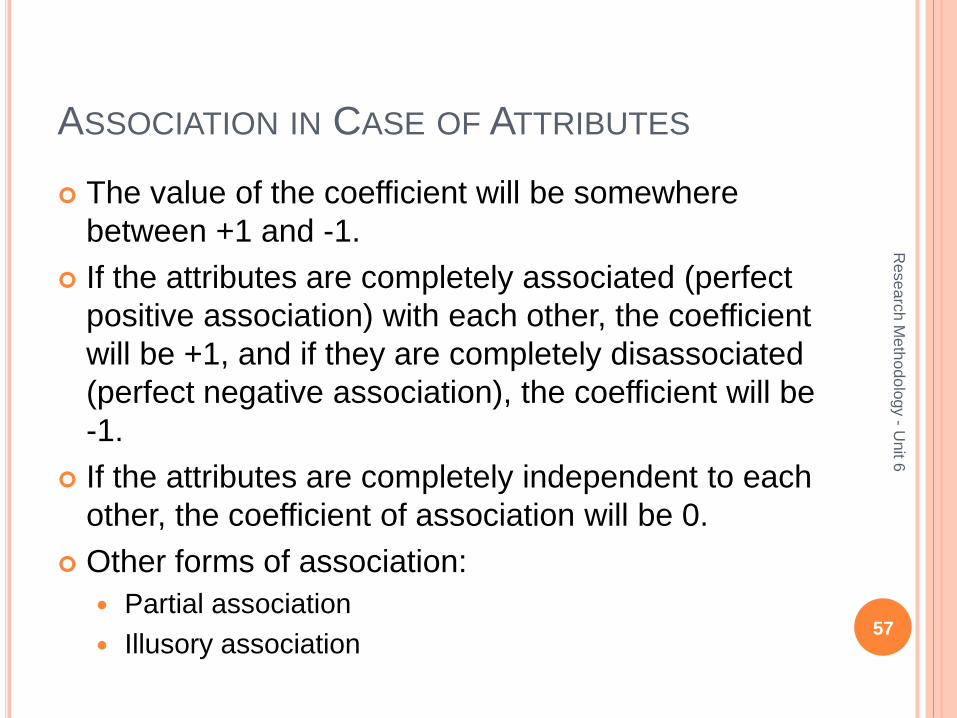
The value of the coefficient will be somewhere

between +1 and -1.

If the attributes are completely associated (perfect

positive association) with each other, the coefficient

will be +1, and if they are completely disassociated

(perfect negative association), the coefficient will be

-1.

If the attributes are completely independent to each

other, the coefficient of association will be 0.

Other forms of association:

Partial association

Illusory association 57

Rese

arc

h M

eth

od

olo

gy -

Unit 6

THE NULL HYPOTHESIS

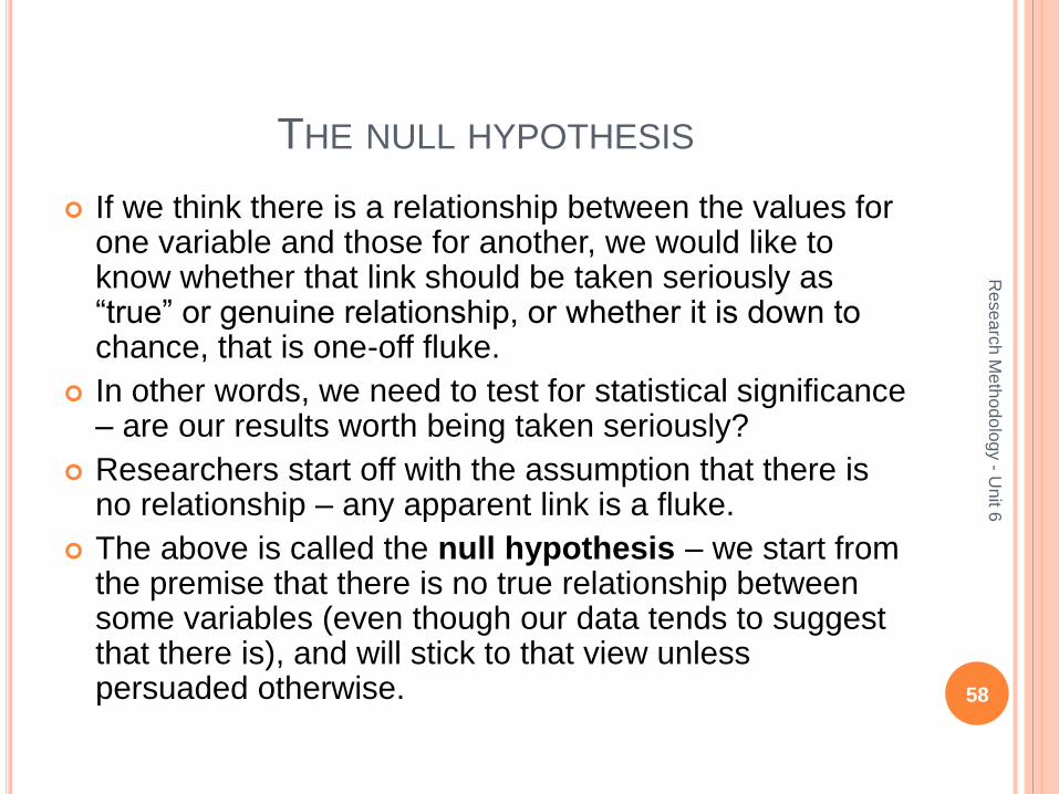
If we think there is a relationship between the values for one variable and those for another, we would like to know whether that link should be taken seriously as “true” or genuine relationship, or whether it is down to chance, that is one-off fluke.

In other words, we need to test for statistical significance – are our results worth being taken seriously?

Researchers start off with the assumption that there is no relationship – any apparent link is a fluke.

The above is called the null hypothesis – we start from the premise that there is no true relationship between some variables (even though our data tends to suggest that there is), and will stick to that view unless persuaded otherwise. 58

Rese

arc

h M

eth

od

olo

gy -

Unit 6

TESTS OF SIGNIFICANCE

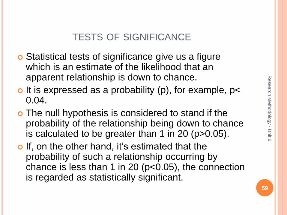
Statistical tests of significance give us a figure which is an estimate of the likelihood that an apparent relationship is down to chance.

It is expressed as a probability (p), for example, p< 0.04.

The null hypothesis is considered to stand if the probability of the relationship being down to chance is calculated to be greater than 1 in 20 (p>0.05).

If, on the other hand, it’s estimated that the probability of such a relationship occurring by chance is less than 1 in 20 (p<0.05), the connection is regarded as statistically significant.

59

Rese

arc

h M

eth

od

olo

gy -

Unit 6

CHI-SQUARE TEST

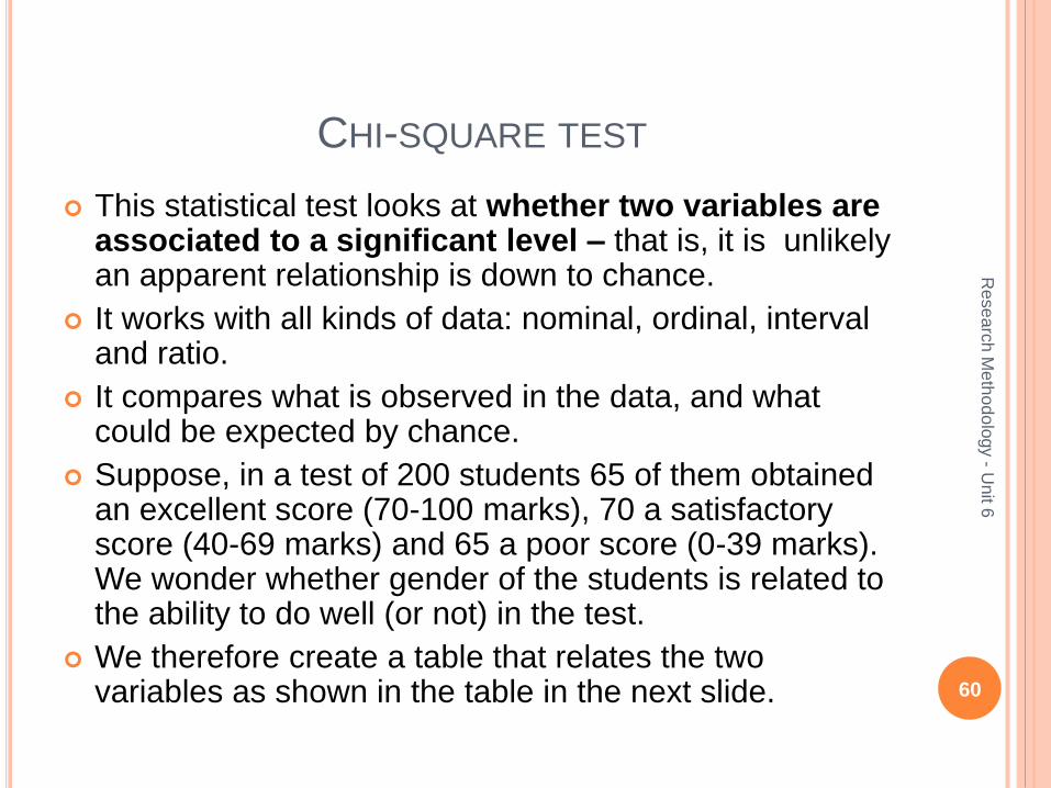
This statistical test looks at whether two variables are associated to a significant level – that is, it is unlikely an apparent relationship is down to chance.

It works with all kinds of data: nominal, ordinal, interval and ratio.

It compares what is observed in the data, and what could be expected by chance.

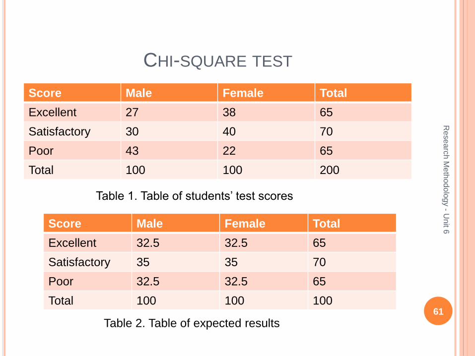
Suppose, in a test of 200 students 65 of them obtained an excellent score (70-100 marks), 70 a satisfactory score (40-69 marks) and 65 a poor score (0-39 marks). We wonder whether gender of the students is related to the ability to do well (or not) in the test.

We therefore create a table that relates the two variables as shown in the table in the next slide. 60

Rese

arc

h M

eth

od

olo

gy -

Unit 6

CHI-SQUARE TEST

Score Male Female Total

Excellent 27 38 65

Satisfactory 30 40 70

Poor 43 22 65

Total 100 100 200

61

Rese

arc

h M

eth

od

olo

gy -

Unit 6

Table 1. Table of students’ test scores

Score Male Female Total

Excellent 32.5 32.5 65

Satisfactory 35 35 70

Poor 32.5 32.5 65

Total 100 100 100

Table 2. Table of expected results

CHI-SQUARE TEST

In our sample of 200 students, we can see that, on

average, males performed worse than females.

Can we draw the conclusion that the same is true

for the broader student population from which our

sample was drawn?

Or did we just happen to get an unrepresentative

sample of students?

How likely is it that we used an untypical sample of

students drawn, by chance, from a student

population where there is no relationship between

gender and performance?62

Rese

arc

h M

eth

od

olo

gy -

Unit 6

CHI-SQUARE TEST

The chi-square test can be used to find out the

likelihood of us having an unrepresentative sample

by chance.

If there was no association between gender and

performance in the test, we would expect the table

to look like as shown in Table2.

The chi-square test performs a set of calculations

using the difference between the expected values

as shown in Table 2 and the actual values as

shown in Table 1.

For our example, a computer program would

calculate chi-square as 10.07. 63

Rese

arc

h M

eth

od

olo

gy -

Unit 6

CHI-SQUARE TEST

Degrees of freedom

Significa

nce

level

1 2 3 4 5 6 7 8

p < 0.1 2.71 4.00 6.25 7.78 9.24 10.64 12.02 13.36

p < 0.05 3.84 5.99 7.81 9.49 11.07 12.59 14.07 15.51

p < 0.01 6.63 9.21 11.34 13.28 15.09 16.81 18.48 20.09

p <

0.001

10.83 13.82 16.27 18.47 20.52 22.46 24.32 26.12

64

Rese

arc

h M

eth

od

olo

gy -

Unit 6

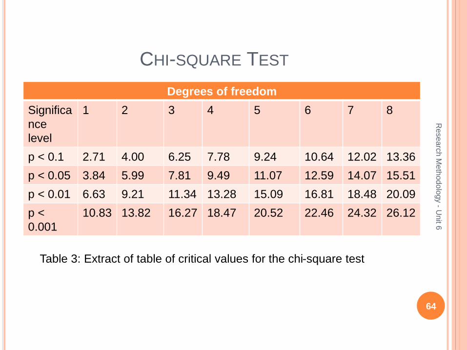
Table 3: Extract of table of critical values for the chi-square test

CHI-SQUARE TEST

For using the value from the table of critical values for chi-square, and find out whether we have confidence that the observed relationship in the sample is not due to chance, we also need to know the characteristics of the table used, based on the number of columns and rows that had data values in them (don’t include the ‘total’ row and column, as these are just a check, not data).

This is known as table’s degrees of freedom.

The degree of freedom is (R-1) x (C-1) where R is the number of rows and C the number of columns, which is (3-1)x (2-1)=2 degrees of freedom.

65

Rese

arc

h M

eth

od

olo

gy -

Unit 6

CHI-SQUARE TEST

Tables of critical values for chi-squared typically shows degrees of freedom against probability.

Table 3 gives an extract of such a table.

Look for the chi-squared value in the table for 2 degrees of freedom.

We see that for significance at the 0.05 level, chi-squared would have to be at least 5.99 and for significance at the 0.01 level, it would have to be at least 9.21.

So, we can assert that the probability of getting by chance a sample with the association we’ve found between gender and performance is less that 1 in 100 (p<0.01).

As we normally look for at least p<0.05, the connection is regarded as statistically significant.

The chi-square test can be only used where there is sufficiently large data set ( at least 30 in the sample), and a minimum value of in each table cell.

66

Rese

arc

h M

eth

od

olo

gy -

Unit 6

OTHER TESTS FOR SIGNIFICANCE

T-test

67

Rese

arc

h M

eth

od

olo

gy -

Unit 6

End of Unit 6

68

Rese

arc

h M

eth

od

olo

gy -

Unit 6

Research methodology unit6

Education

Transcript of Research methodology unit6