research-information.bristol.ac.ukresearch-information.bristol.ac.uk/files/69264440/BuiKeatingSmith... ·...

Bui, H. M., Keating, J. P., & Smith, D. J. (2016). On the variance of sums ofarithmetic functions over primes in short intervals and pair correlation for L-functions in the Selberg class. Journal of the London Mathematical Society,94(1), 161-185. DOI: 10.1112/jlms/jdw030

Peer reviewed version

Link to published version (if available):10.1112/jlms/jdw030

Link to publication record in Explore Bristol ResearchPDF-document

This is the accepted author manuscript (AAM). The final published version (version of record) is available onlinevia London Mathematical Society at DOI: 10.1112/jlms/jdw030. Please refer to any applicable terms of use ofthe publisher.

University of Bristol - Explore Bristol ResearchGeneral rights

This document is made available in accordance with publisher policies. Please cite only the publishedversion using the reference above. Full terms of use are available:http://www.bristol.ac.uk/pure/about/ebr-terms

https://doi.org/10.1112/jlms/jdw030

https://research-information.bristol.ac.uk/en/publications/on-the-variance-of-sums-of-arithmetic-functions-over-primes-in-short-intervals-and-pair-correlation-for-lfunctions-in-the-selberg-class(1da8c3ea-07ad-4923-8a3e-077358781c55).html

https://research-information.bristol.ac.uk/en/publications/on-the-variance-of-sums-of-arithmetic-functions-over-primes-in-short-intervals-and-pair-correlation-for-lfunctions-in-the-selberg-class(1da8c3ea-07ad-4923-8a3e-077358781c55).html

Take down policy

Explore Bristol Research is a digital archive and the intention is that deposited content should not beremoved. However, if you believe that this version of the work breaches copyright law please [email protected] and include the following information in your message:

• Your contact details• Bibliographic details for the item, including a URL• An outline of the nature of the complaint

On receipt of your message the Open Access Team will immediately investigate your claim, make aninitial judgement of the validity of the claim and, where appropriate, withdraw the item in questionfrom public view.

Submitted exclusively to the London Mathematical Societydoi:10.1112/0000/000000

On the variance of sums of arithmetic functions over primes inshort intervals and pair correlation for L-functions in the Selberg

class

H. M. Bui, J. P. Keating and D. J. Smith

Abstract

We establish the equivalence of conjectures concerning the pair correlation of zeros of L-functionsin the Selberg class and the variances of sums of a related class of arithmetic functions over primesin short intervals. This extends the results of Goldston & Montgomery [6] and Montgomery &Soundararajan [10] for the Riemann zeta-function to other L-functions in the Selberg class. Ourapproach is based on the statistics of the zeros because the analogue of the Hardy-Littlewoodconjecture for the auto-correlation of the arithmetic functions we consider is not available ingeneral. One of our main findings is that the variances of sums of these arithmetic functions overprimes in short intervals have a different form when the degree of the associated L-functions is 2or higher to that which holds when the degree is 1 (e.g. the Riemann zeta-function). Specifically,when the degree is 2 or higher there are two regimes in which the variances take qualitativelydifferent forms, whilst in the degree-1 case there is a single regime.

1. Introduction

Let Λ(n) denote the von Mangoldt function, defined by

Λ(n) =

{log p if n = pk for some prime p and integer k ≥ 1,

0 otherwise.

The prime number theorem implies that

ψ(x) :=∑n≤x

Λ(n) = x+ o(x)

as x→∞, and so determines the average of Λ(n) over long intervals. In many problems oneneeds to understand sums over shorter intervals. This is more difficult, because the fluctuationsin their values can be large. To this end Goldston and Montgomery [6] initiated the study ofthe variances

V (X, δ) :=

∫X1

(ψ(x+ δx)− ψ(x)− δx

)2dx (1.1)

and

V (X,h) :=

∫X1

(ψ(x+ h)− ψ(x)− h

)2dx. (1.2)

For example, they put forward the following conjecture [6]:

2000 Mathematics Subject Classification 11N05, 11M41, 11M26.

We gratefully acknowledge supports from the Leverhulme Trust and the EPSRC Programme GrantEP/K034383/1 LMF: L-Functions and Modular Forms. The second author is also funded by a Royal SocietyWolfson Research Merit Award and a Royal Society Leverhulme Senior Research Fellowship.

of 25 H. M. BUI, J. P. KEATING AND D. J. SMITH

Conjecture 1 (Variance of primes in short intervals). For any fixed ε > 0

V (X,h) ∼ hX(

logX − log h)

uniformly for 1 ≤ h ≤ X1−ε.

This conjecture remains open, but its analogue in the function field setting has recently beenproved in the limit of large field size [7].

It is natural to try to compute the variances (1.1) and (1.2) using the Hardy-LittlewoodConjecture for the auto-correlation of Λ(n):∑

n≤X

Λ(n)Λ(n+ k) ∼ S(k)X (1.3)

as X →∞, where S(k) is the singular series

S(k) =

2∏p>2

(1− 1

(p−1)2

)∏p>2p|k

p−1p−2 if k is even,

0 if k is odd.

Averaging over k up to h in (1.3), subject to an assumption concerning the implicit error term,Montgomery and Soundararajan [10] established a more precise asymptotic for the varianceV (X,h) when logX ≤ h ≤ X1/2:

V (X,h) = hX(

logX − log h− γ0 − log 2π)

+Oε

(h15/16X(logX)17/16 + h2X1/2+ε

), (1.4)

where γ0 is the Euler-Mascheroni constant.An alternative approach to computing the variances (1.1) and (1.2) is based on the connection

with the Riemann zeta-function ζ(s) via

ζ ′(s)

ζ(s)= −

∞∑n=1

Λ(n)

ns.

This links statistical properties of Λ(n) to those of the zeros of the Riemann zeta-function.Specifically, Goldston and Montgomery [6] proved that Conjecture 1 is equivalent to thefollowing conjecture, due to Montgomery [9], concerning the pair correlation of the non-trivialzeros 1

2 + iγ of the Riemann zeta-function (in writing the zeros in this form one is assumingthe Riemann Hypothesis):

Conjecture 2 (Pair Correlation Conjecture). Let

F(X,T ) =∑

0<γ,γ′≤T

Xi(γ−γ′)w(γ − γ′),

where w(u) = 44+u2 . Then for any fixed A ≥ 1 we have

F(X,T ) ∼ T log T

2π

uniformly for T ≤ X ≤ TA.

The equivalence between Conjecture 1 and Conjecture 2 has been investigated further in [3,8] to include the lower order terms.

We have two main goals in this paper. The first is to show how the more precise formula(1.4) follows from a more accurate expression for the pair correlation of the Riemann zerosproposed by Bogomolny and Keating [2] (see also [1]):

SUMS OF ARITHMETIC FUNCTIONS OVER SHORT INTERVALS Page 3 of 25

Conjecture 3. For h a suitable even test function∑0<γ,γ′≤T

h(γ − γ′) =h(0)

2π

∫T0

logt

2πdt+

1

(2π)2

∫T0

∫T−T

h(η)

[(log

t

2π

)2

+2

((ζ ′

ζ

)′(1 + iη) +

(t

2π

)−iηA(iη)ζ(1− iη)ζ(1 + iη)−B(iη)

)]dηdt+Oε(T

1/2+ε),

where

A(r) =∏p

(1− 1p1+r )(1− 2

p + 1p1+r )

(1− 1p )2

and

B(r) =∑p

(log p

p1+r − 1

)2

.

Here the integral is to be regarded as a principal value near η = 0.

This formula was originally obtained in [2] from the Hardy-Littlewood Conjecture (1.3).Importantly for us here, it was shown by Conrey and Snaith [5] to follow from the ratiosconjecture for the Riemann zeta-function [4], and in the above formulation we use theirnotation. It follows from our general results, set out below, that (1.4) may be obtained froman analysis based on Conjecture 3.

The second goal of this paper, and in fact our principal goal, is to extend the approach basedon formulae like that in Conjecture 3 to a wider class of sums in which the von Mangoldtfunction is multiplied by arithmetic functions associated with other L-functions in the Selbergclass [14]. This essentially corresponds to studying the variances of these functions whensummed over prime arguments in short intervals.

Let S denote the Selberg class L-functions. For F ∈ S primitive,

F (s) =

∞∑n=1

aF (n)

ns,

let mF ≥ 0 be the order of the pole at s = 1,

F ′

F(s) = −

∞∑n=1

ΛF (n)

nsand F (s)−1 =

∞∑n=1

µF (n)

ns(Re(s) > 1).

The function F (s) has an Euler product

F (s) =∏p

exp

( ∞∑l=1

bF (pl)

pls

)(1.5)

and satisfies a functional equation

Φ(s) = εFΦ(1− s),

where

Φ(s) = Qs( r∏j=1

Γ(λjs+ µj)

)F (s),

with some Q > 0, λj > 0, Re(µj) ≥ 0 and |εF | = 1. Here Φ(s) = Φ(s). We will also write thefunctional equation in the form

F (s) = X(s)F (1− s),


where

X(s) = εFQ1−2s

r∏j=1

Γ(λj(1− s) + µj

)Γ(λjs+ µj)

.

The two important invariants of F (s) are the degree dF and the conductor qF ,

dF = 2

r∑j=1

λj and qF = (2π)dFQ2r∏j=1

λ2λj

j .

For F ∈ S, it is expected that a generalised prime number theorem of the form

ψF (x) :=∑n≤x

ΛF (n) = mFx+ o(x)

holds. In analogy with (1.1) and (1.2) we shall consider

VF (X, δ) :=

∫X1

∣∣∣ψF (x+ δx)− ψF (x)−mF δx∣∣∣2dx

and

VF (X,h) :=

∫X1

∣∣∣ψF (x+ h)− ψF (x)−mFh∣∣∣2dx.

So, for example, when F represents an L-function associated with an elliptic curve, VF (X, δ)and VF (X,h) represent the variances of sums over short intervals involving the Fouriercoefficients of the associated modular form evaluated at primes and prime powers; and in thecase of Ramanujan’s L-function, they represent the corresponding variances for sums involvingthe Ramanujan τ -function.

It is important to note that for most F ∈ S one does not expect an analogue of the Hardy-Littlewood Conjecture (1.3); that is, for most F ∈ S it is expected that∑

n≤X

ΛF (n)ΛF (n+ k) = o(X).

This might lead one to anticipate that VF (X, δ) and VF (X,h) typically exhibit differentasymptotic behaviour than in the case when F is the Riemann zeta-function, because (1.3)plays a central role in our understanding of the variances in that case. Somewhat surprisinglyfrom this perspective, our results suggest that VF (X, δ) and VF (X,h) have the same generalform for all F ∈ S. The reason is that they all look essentially the same from the perspectiveof the statistical distribution of their zeros. It would be interesting to understand this from theHardy-Littlewood point of view. In the average over k up to h it appears that the terms thatare o(x) fail to contribute for small h, however for sufficiently large h there is a regime changedue to errors in the singular series conspiring in the long average, giving a transition. Drawingattention to this is one of our principal motivations.

The pair correlation of zeros of F (s) is defined in analogy with the expression in Conjecture2 as

FF (X,T ) =∑

−T≤γF ,γ′F≤T

Xi(γF−γ′F )w(γF − γ′F ),

where, assuming the Generalized Riemann Hypothesis (GRH), the non-trivial zeros of F (s)are denoted 1

2 + iγF . Murty and Perelli [11] conjectured that

FF (X,T ) ∼ T logX

π

uniformly for TA1 ≤ X ≤ TA2 for any fixed 0 < A1 ≤ A2 ≤ dF , and

FF (X,T ) ∼ dFT log T

π


uniformly for TA1 ≤ X ≤ TA2 for any fixed dF ≤ A1 ≤ A2 <∞.Our approach to studying the variances VF (X, δ) and VF (X,h) is based on the pair

correlation of zeros. Specifically, our main results are as stated below. We set out these resultsin pairs, because, unlike the case of the Riemann zeta-function and other degree-1 L-functions,when dF ≥ 2 there are two cases to consider: either T ≤ X ≤ T dF or T dF ≤ X. In both of thesecases, our results then correspond to examining the implication of the pair correlation of zerosfor VF (X, δ) (Theorems labelled A), the implications in the reverse direction (B), implicationsof VF (X, δ) for VF (X,h) (C), and in the reverse direction (D).

Theorem A1. Assume GRH. If dF < A1 < A2 <∞ and

FF (X,T ) =T

π

(dF log

T

2π+ log qF − dF

)+O

(T 1−c) (1.6)

uniformly for TA1 � X � TA2 for some c > 0, then for any fixed 1/A2 < B1 ≤ B2 < 1/A1 wehave

VF (X, δ) =1

2δX2

(dF log

1

δ+ log qF + (1− γ0 − log 2π)dF

)+O

(δ1+c/2X2

)+Oε

(δ1−εX2(δX1/A2)1/2

)+Oε

(δ1−εX2(δX1/A1)−2A1/(4A1+1)

)uniformly for X−B2 � δ � X−B1 .

Theorem A2. Assume GRH. If 1 < A1 < A2 < dF and

FF (X,T ) =T logX

π+O

(T 1−c)

uniformly for TA1 � X � TA2 for some c > 0, then for any fixed 1/A2 < B1 ≤ B2 < 1/A1 wehave

VF (X, δ) =1

6δX2

(3 logX − 4 log 2

)+O

(δ1+c/2X2

)+Oε

(δ1−εX2(δX1/A2)1/2

)+Oε

(δ1−εX2(δX1/A1)−2A1/(4A1+1)

)uniformly for X−B2 � δ � X−B1 .

Theorem B1. Assume GRH. If 0 < B1 < B2 < 1/dF and

VF (X, δ) =1

2δX2

(dF log

1


)+O

(δ1+cX2

)(1.7)

uniformly for X−B2 � δ � X−B1 for some c > 0, then for any fixed 1/B2 < A1 ≤ A2 < 1/B1

we have

FF (X,T ) =T

π

(dF log

T

2π+ log qF − dF

)+Oε

(T 3/(3+c)+ε

)+Oε

(T 1+ε

(T/XB2

)2)+Oε

(T 1+ε

(T/XB1

)−1/4)uniformly for TA1 � X � TA2 .

Theorem B2. Assume GRH. If 1/dF < B1 < B2 < 1 and

VF (X, δ) =1

6δX2

(3 logX − 4 log 2

)+O

(δ1+cX2

)


uniformly for X−B2 � δ � X−B1 for some c > 0, then for any fixed 1/B2 < A1 ≤ A2 < 1/B1

we have

FF (X,T ) =T logX

π+Oε

(T 3/(3+c)+ε

)+Oε

(T 1+ε

(T/XB2

)2)+Oε

(T 1+ε

(T/XB1

)−1/4)uniformly for TA1 � X � TA2 .

Theorem C1. Assume GRH. If 0 < B1 < B2 ≤ B3 < 1/dF and

VF (X, δ) =1

2δX2

(dF log

1


)+O

(δ1+cX2

)(1.8)

uniformly for X−B3 � δ � X−B1 for some c > 0, then we have

VF (X,h) = hX(dF log

X

h+ log qF − (γ0 + log 2π)dF

)+Oε

(hX1+ε(h/X)c/3

)+Oε

(hX1+ε

(hX−(1−B1)

)1/3(1−B1))

(1.9)

uniformly for X1−B3 � h� X1−B2 .

Theorem C2. Assume GRH. If 1/dF < B1 < B2 ≤ B3 < 1 and

VF (X, δ) =1

6δX2

(3 logX − 4 log 2

)+O

(δ1+cX2

)uniformly for X−B3 � δ � X−B1 for some c > 0, then we have

VF (X,h) =1

6hX(

6 logX −(3 + 8 log 2

))+Oε

(hX1+ε(h/X)c/3

)+Oε

(hX1+ε

(hX−(1−B1)

)1/3(1−B1))

uniformly for X1−B3 � h� X1−B2 .

Theorem D1. Assume GRH. If 0 < B1 ≤ B2 < B3 < 1/dF and

VF (X,h) = hX(dF log

X

h+ log qF − (γ0 + log 2π)dF

)+O

(hX1−c)

uniformly for X1−B3 � h� X1−B1 for some c > 0, then we have

VF (X, δ) =1

2δX2

(dF log

1


)+Oε

(δ1−εX2−c/3)+Oε

(δ1−εX2

(δXB3

)−2/3B3)

uniformly for X−B2 � δ � X−B1 .

Theorem D2. Assume GRH. If 1/dF < B1 ≤ B2 < B3 < 1 and

VF (X,h) =1

6hX(

6 logX −(3 + 8 log 2

))+O

(hX1−c)

uniformly for X1−B3 � h� X1−B1 for some c > 0, then we have

VF (X, δ) =1

6δX2

(3 logX − 4 log 2

)+Oε

(δ1−εX2−c/3)+Oε

(δ1−εX2

(δXB3

)−2/3B3)

uniformly for X−B2 � δ � X−B1 .


Remark 1. The main motivation for proving these theorems comes from the fact, shownin Sections 3 and 4, that the Selberg Orthogonality Conjecture and the ratios conjecture [4,5] for F ∈ S imply that

FF (Tα, T ) =

{T logXπ +Oε(T

α/dF+ε) +Oε(T1/2+ε) if α < dF ,

Tπ log qFT

dF

(2π)dF− dFT

π +Oε(T1/2+ε) if α > dF ,

for a smoothed form of the pair correlation FF (X,T ) defined by

FF (X,T ) =∑


Xi(γF−γ′F )e−(γF−γ′F )2 .

We expect that FF (X,T ) and FF (X,T ) satisfy the same estimates, at least up to somepower saving error term, and these are the forms that appear in the theorems quoted above.Alternatively, if we were to replace FF (X,T ) by FF (X,T ) in the statements of the abovetheorems, we would obtain correspondingly smoothed forms of the variances VF (X, δ) andVF (X,h) instead; that is, variances involving averages with weight-functions whose mass isconcentrated on (1, X). We establish the form of the ratios conjecture we need in Section 3and from this obtain the above formulae for FF (X,T ) in Section 4.

Figure 1. VF (X,h)/(hX) plotted against log h when F is the Riemann zeta-function andX = 15000000 (•). The line is given by y = −x+ log 15000000− γ0 − log 2π, which

corresponds to dF = 1 and qF = 1.

Remark 2. We draw attention in particular to the fact that when dF = 1 our theoremsdescribe only one regime, but when dF ≥ 2 a new regime (described, for example, by TheoremA2) comes into play; the variances when dF ≥ 2 are therefore qualitatively different to whendF = 1. We illustrate this in two figures, which show data from numerical computations. Inboth cases we plot VF (X,h)/(hX) against log h, for a fixed value of X as h varies and overlaythe straight lines coming from the formulae for the variances described in the above theorems.


In the first case, shown in Figure 1 above, F is the Riemann zeta-function (so ΛF is just thevon Mangoldt function) and X = 15000000. This is, of course, an example with dF = 1 and soone sees a single regime that is well described by (1.4).

By way of contrast, we plot in Figure 2 data for two L-functions with dF = 2. In theseexamples X = 1000000. The lines correspond to the formulae for the two regimes described byTheorems C1 and C2.

Figure 2. VF (X,h)/(hX) plotted against log h when F is associated with the Ramanujanτ -function (•) and with an elliptic curve of conductor 37 (N). Here X = 1000000. The

horizontal line is given by y = log 1000000− (3+8 log 2)6 . The slanted lines are given by

y = −2x+ 2(log 1000000− γ0 − log 2π), which corresponds to the case dF = 2 and qF = 1 forthe Ramanujan τ -function, and y = −2x+ 2(log 1000000− γ0 − log 2π) + log 37, which

corresponds to the case dF = 2 and qF = 37 for the elliptic curve.

Remark 3. The analogues of Theorems A1, B1, C1 and D1 in the case when F is theRiemann zeta-function were obtained by Chan [3]. Note that, unlike the case of the Riemannzeta-function [6, 3], the A Theorems above are not exactly the converse of the B Theorems,and the C Theorems are not exactly the converse of the D Theorems. They are close to beingthe converse of each other, but with the power saving errors we have here, the intervals ofuniformity do not match precisely.

The proofs of the theorems within each pair are essentially identical, so we only give theproofs of Theorems A1, B1 and C1. Likewise, the proofs of Theorems D1 and D2 are similarto the proofs of C1 and C2, so we omit them too.


2. Auxiliary lemmas

Lemma 2.1. Suppose f is a non-negative function with f(t)�ε |t|ε. If∫T−T

f(t)dt = T(

log T +A)

+O(T 1−c)

uniformly for κ−(1−c1) ≤ T ≤ κ−(1+c2) for some A ∈ R and 0 < c, c1, c2 < 1, then

I(κ) :=

∫∞−∞

(sinκu

u

)2

f(u)du =π

2κ(

log1

κ+B

)+O

(κ1+c

)+Oε

(κ1+c1−ε

)+Oε

(κ1+c2−ε

)as κ→ 0+, with B = A+ 2− γ0 − log 2.

Proof. As in the proof of Lemma 2 of Goldston and Montgomery [6], we write

I(κ) =

( ∫U1

−U1

)+

( ∫−U1

−U2

+

∫U2

U1

)+

( ∫−U2

−∞+

∫∞U2

)= I1(κ) + I2(κ) + I3(κ),

say, where

U1 = κ−(1−c1) and U2 = κ−(1+c2).

Since f(t)�ε |t|ε, we have

I1(κ)�ε

∫U1

−U1

κ2|u|εdu�ε κ2U1+ε

1 �ε κ1+c1−ε. (2.1)

Similarly,

I3(κ)�ε

∫∞U2

u−2+εdu�ε U−1+ε2 �ε κ

1+c2−ε. (2.2)

To treat I2(κ) we let

r(t) = f(t) + f(−t)−(

log t+A+ 1)

and

R(u) =

∫u0

r(t)dt =

∫u0

(f(t) + f(−t)

)dt− u

(log u+A

).

Then R(u)� u1−c uniformly for U1 ≤ u ≤ U2, and

I2(κ) =

∫U2

U1

(sinκu

u

)2(f(u) + f(−u)

)du

=

∫U2

U1

(sinκu

u

)2(log u+A+ 1

)du+

∫U2

U1

(sinκu

u

)2

dR(u).

Integrating by parts, the second integral is

� κ2R(U1) + U−22 R(U2) +

∫U2

U1

∣∣R(u)∣∣(∣∣∣∣κ sin 2κu

u2

∣∣∣∣+

∣∣∣∣ (sinκu)2

u3

∣∣∣∣)du� κ1+c.

For the first integral, we extend the range of integration to [0,∞). As in the treatment forI1(κ) and I3(κ), this introduces an error term of size �ε κ

1+c1−ε + κ1+c2−ε. Hence

I2(κ) =

∫∞0

(sinκu

u

)2(log u+A+ 1

)du+O

(κ1+c

)+Oε

(κ1+c1−ε

)+Oε

(κ1+c2−ε

). (2.3)


In view of (2.1)–(2.3) we are left to estimate the main term, which is

κ

∫∞0

(sinu

u

)2(log u+ log

1

κ+A+ 1

)du

=π

2

(1− γ0 − log 2

)κ+

π

2κ(

log1

κ+A+ 1

)=π

2κ(

log1

κ+A+ 2− γ0 − log 2

),

and the lemma follows.

Lemma 2.2. Suppose f, g are non-negative functions with f(t)�ε |t|ε. If

I(κ) :=

∫∞−∞

(sinκu

u

)2

f(u)du =π

2κ(

log1

κ+B

)+O

(κ1+cg(T )

)uniformly for T−(1+c1) ≤ κ ≤ T−(1−c2) for some B ∈ R and 0 < c, c1, c2 < 1, then∫T

−Tf(t)dt = T

(log T +A

)+Oε

((T 3g(T )

)1/(3+c)+ε)+Oε

(T 1−2c1+ε

)+Oε

(T 1−c2/4+ε

)as T →∞, with A = B − 2 + γ0 + log 2.

Proof. Let

r(u) = f(u) + f(−u)−(

log u+B − 1 + γ0 + log 2),

and

R(κ) =

∫∞0

(sinκu

u

)2

r(u)du.

Then we have

R(κ) = I(κ)−∫∞0

(sinκu

u

)2(log u+B − 1 + γ0 + log 2

)du

= I(κ)− π

2κ(

log1

κ+B

)� κ1+cg(T ) (2.4)

uniformly for T−(1+c1) ≤ κ ≤ T−(1−c2). Also, since f(t)�ε |t|ε, we get

R(κ)�ε

∫∞0

min{κ2, u−2

}|u|εdu�ε κ

1−ε (2.5)

for all κ ≥ 0.Let

Kη(x) =sin 2πx+ sin 2π(1 + η)x

2πx(1− 4η2x2)

for η > 0. Then

Kη(t) =

1 if |t| ≤ 1,

cos2(π(|t|−1)

2η

)if 1 ≤ |t| ≤ 1 + η,

0 if |t| ≥ 1 + η.

The kernel Kη is even and satisfies the following properties: Kη(x), K ′η(x)→ 0 as x→∞, and[3]

K ′′η (x)� min{

1, η−3|x|−3}. (2.6)


Integrating by parts twice, we have

Kη(t) =

∫∞0

K ′′η (x)

(sinπtx

πt

)2

dx.

This implies that∫∞0

r(t)Kη

( tT

)dt = π−2T 2

∫∞0

K ′′η (x)R(πxT

)dx

= π−2T 2

( ∫T1

0

K ′′ηR+

∫T2

T1

K ′′ηR+

∫∞T2

K ′′ηR

),

where T1 = T−c1 and T2 = T c2 . From (2.5) and (2.6) we have∫T1

0

K ′′ηR�ε

∫T1

0

(x/T )1−εdx�ε T−(1+2c1)+ε

and ∫∞T2

K ′′ηR�ε

∫∞T2

η−3x−3(x/T )1−εdx�ε η−3T−(1+c2)+ε.

Furthermore, (2.4) and (2.6) lead to∫T2

T1

K ′′ηR�∫T2

T1

min{

1, η−3x−3}

(x/T )1+cg(T )dx� η−(2+c)T−(1+c)g(T ).

So ∫∞0

r(t)Kη

( tT

)dt�ε T

1−2c1+ε + η−3T 1−c2+ε + η−(2+c)T 1−cg(T ).

Hence∫∞−∞

f(t)Kη

( tT

)dt =

∫∞0

(log t+B − 1 + γ0 + log 2

)Kη

( tT

)dt

+Oε(T 1−2c1+ε

)+Oε

(η−3T 1−c2+ε) +O

(η−(2+c)T 1−cg(T )

)=

∫T0

(log t+B − 1 + γ0 + log 2

)dt+O

( ∫ (1+η)TT

log tdt

)+Oε

(T 1−2c1+ε

)+Oε

(η−3T 1−c2+ε) +O

(η−(2+c)T 1−cg(T )

)= T (log T +B − 2 + γ0 + log 2) +Oε

(ηT 1+ε

)+Oε

(T 1−2c1+ε

)+Oε

(η−3T 1−c2+ε) +O

(η−(2+c)T 1−cg(T )

),

and we obtain the lemma.

Lemma 2.3. Suppose f is a non-negative function. If∫∞−∞

f(T + y)e−2|y|dy = 1 +O(e−cY

)for Y ≤ T ≤ Y + log 2 for some c > 0, then∫ log 2

0

f(Y + y)e2ydy =3

2+O

(e−cY/2

).

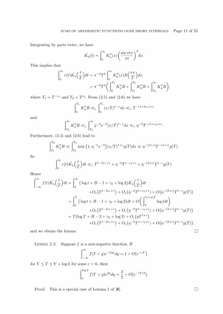
Proof. This is a special case of Lemma 1 of [8].


Lemma 2.4. Assume GRH. We have∫X1

∣∣∣ψF (x+ δx)− ψF (x)−mF δx∣∣∣2dx� δX2

(log

2

δ

)2(2.7)

for 0 < δ ≤ 1, and ∫X1

∣∣∣ψF (x+ h)− ψF (x)−mFh∣∣∣2dx� hX

(log

2X

h

)2(2.8)

for 0 < h ≤ X.

Proof. The argument is identical to that of Saffari and Vaughan in [13].

3. Ratios conjecture for L-functions in the Selberg class

This section and the following one concerning the pair correlation of zeros of L-functions inthe Selberg class are deeply heuristic in that they make essential use of the ratios conjecturefor L-functions. Interested readers unfamiliar with the “recipe” that leads to this conjectureare referred to, for example, [5; Sections 2 and 4] for details.

We would like to study

RF (α, β, γ, δ) =

∫T−T

F (s+ α)F (1− s+ β)

F (s+ γ)F (1− s+ δ)dt,

where s = 1/2 + it, using the recipe in [4, 5]. The shifts are constrained as follows:∣∣Re(α)∣∣, ∣∣Re(β)

∣∣ < 1

4,

(log T )−1 � Re(γ),Re(δ) <1

4(3.1)

Im(α), Im(β), Im(γ), Im(δ)�ε T1−ε.

We use the approximate functional equation for the L-functions in the numerator,

F (s) =∑n

aF (n)

ns+X(s)

∑n

aF (n)

n1−s,

and the normal Dirichlet series expansion for those in the denominator,

F (s)−1 =∑n

µF (n)

ns.

As we integrate term-by-term, only the pieces with the same number of X(s) as X(1− s)contribute to the main terms.

The terms from the first part of each approximate functional equation yield

2T∑

hm=kn

aF (m)aF (n)µF (h)µF (k)

m1/2+αn1/2+βh1/2+γk1/2+δ

= 2T∏p

( ∑h+m=k+n

aF (pm)aF (pn)µF (ph)µF (pk)

p(1/2+α)m+(1/2+β)n+(1/2+γ)h+(1/2+δ)k

).

We note that the functions aF (n), µF (n) are multiplicative because of the existence of theEuler product (1.5), and

bF (p) = aF (p) = −µF (p).


Hence the above expression is

2TAF (α, β, γ, δ)(F ⊗ F )(1 + α+ β)(F ⊗ F )(1 + γ + δ)

(F ⊗ F )(1 + α+ δ)(F ⊗ F )(1 + β + γ),

where AF (α, β, γ, δ) is an arithmetical factor given by some Euler product that is absolutelyand uniformly convergent in some product of fixed half-planes containing the origin,

AF (α, β, γ, δ) =∏p

( ∑h+m=k+n


p(1/2+α)m+(1/2+β)n+(1/2+γ)h+(1/2+δ)k

)(3.2)

exp

( ∞∑l=1

l∣∣bF (pl)

∣∣2( 1

pl(1+α+δ)+

1

pl(1+β+γ)− 1

pl(1+α+β)− 1

pl(1+γ+δ)

)).

Here for any F,G ∈ S, we define the tensor product F ⊗G as in [12]

(F ⊗G)(s) =∏p

exp

( ∞∑l=1

lbF (pl)bG(pl)

pls

).

The contribution of the terms coming from the second part of each approximate functionalequation is similar to the first piece except that α is replaced by −β, and β is replaced by −α.Also, because of the factor X(s), we have an extra factor of

X(s+ α)X(1− s+ β) =(qF (|t|+ 2)dF

(2π)dF

)−(α+β)(1 +O

( 1

|t|+ 2

)).

Thus the recipe leads to the following ratios conjecture:

Conjecture 4. With α, β, γ and δ satisfying (3.1) we have

RF (α, β, γ, δ) =

∫T−T

(AF (α, β, γ, δ)

(F ⊗ F )(1 + α+ β)(F ⊗ F )(1 + γ + δ)

(F ⊗ F )(1 + α+ δ)(F ⊗ F )(1 + β + γ)

+(qF (|t|+ 2)dF

(2π)dF

)−(α+β)AF (−β,−α, γ, δ) (F ⊗ F )(1− α− β)(F ⊗ F )(1 + γ + δ)

(F ⊗ F )(1− α+ γ)(F ⊗ F )(1− β + δ)

)dt

+Oε(T1/2+ε),

where AF (α, β, γ, δ) is defined as in (3.2).

We next investigate the analytic properties of (F ⊗ F )(s) at s = 1. We have

(F ⊗ F )′

(F ⊗ F )(s) = −

∑p

∞∑l=1

l2|bF (pl)|2(log p)

pls= −

∑p

|bF (p)|2(log p)

ps+O(1)

= −∑p

|aF (p)|2(log p)

ps+O(1), (3.3)

provided that Re(s) > 12 . Let

S(x) =∑p≤x

|aF (p)|2

p.

The Selberg Orthogonality Conjecture says that

S(x) = log log x+O(1).


So for σ0 > 0 and |σ − σ0| ≤ σ0/2 (σ ∈ C), partial summation gives∑p≤x

|aF (p)|2

p1+σ= O

(log log x

xRe(σ)

)+ σ

∫x1

S(t)

tσ+1dt = O

(log log x

xRe(σ)

)+O(1) + σ

∫x1

log log t

tσ+1dt.

Taking x→∞ we obtain∑p

|aF (p)|2

p1+σ= O(1) + σ

∫∞1

log log t

tσ+1dt = O(1)− (γ0 + log σ) = O(1)− log σ.

Hence using Cauchy’s theorem we get∑p

|aF (p)|2(log p)

p1+σ0=

1

σ0+O(1).

It follows from (3.3) that (F ⊗ F )(s) has a simple pole at s = 1.Note that for a function f(u, v) analytic at (u, v) = (α, α), a simple calculation shows that

d

dα

f(α, γ)

(F ⊗ F )(1− α+ γ)

∣∣∣∣γ=α

=f(α, α)

rF⊗F,

where rF⊗F is the residue of (F ⊗ F ) at s = 1. It is also easy to verify that AF (α, β, α, β) = 1.So taking the derivatives of the expressions in Conjecture 4 with respect to α, β and settingγ = α, δ = β we have

Conjecture 5. With α and β satisfying (3.1) we have∫T−T

F ′

F(s+ α)

F′

F(1− s+ β)dt =

∫T−T

(((F ⊗ F )′

(F ⊗ F )

)′(1 + α+ β)

+1

r2F⊗F

(qF (|t|+ 2)dF

(2π)dF

)−(α+β)AF (−β,−α, α, β)(F ⊗ F )(1− α− β)(F ⊗ F )(1 + α+ β)

+∂2

dαdβAF (α, β, γ, δ)

∣∣∣∣γ=α,δ=β

)dt+Oε(T

1/2+ε),

where AF (α, β, γ, δ) is defined as in (3.2).

4. Pair correlation of zeros of L-functions in the Selberg class

4.1. The pair correlation function

Let F ∈ S. We want to evaluate the sum

S(F ) =∑


h(γF − γ′F ).

We follow the approach in [5] and compute this using contour integrals. Let 1/2 < a < 1and C be the positively oriented rectangle with vertices at 1− a− iT , a− iT , a+ iT and1− a+ iT . Then

S(F ) =1

(2πi)2

∫C

∫C

F ′

F(u)

F ′

F(v)h

(− i(u− v)

)dudv.

The horizontal contributions are small and can be ignored. We denote

S(F ) = I1 + I2 + 2I3 +Oε(Tε),


where I1 has vertical parts a and a, I2 has vertical parts 1− a and 1− a, and I3 has verticalparts a and 1− a.

Using GRH and moving the contours to the right of 1 we have I1 = Oε(Tε).

For I2 we use the functional equation

F ′

F(s) =

X ′

X(s)− F

′

F(1− s). (4.1)

Here

X ′

X(s) = −2 logQ−

r∑j=1

λj

(Γ′

Γ

(λjs+ µj

)+

Γ′

Γ

(λj(1− s) + µj

))= − log

qF (|t|+ 2)dF

(2π)dF+O

(1

|t|+ 2

).

We apply (4.1) to both F ′/F (u) and F ′/F (v). For the terms involving F′/F (1− u) or F

′/F (1−

v), we move the corresponding contour to the right of 1, and as in the treatment for I1, we getOε(T

ε). For the term with X ′/X(u) and X ′/X(v), we move both contours to Re(u) = Re(v) =12 . Again that introduces an error term of size Oε(T

ε). Hence

I2 =1

(2π)2

∫T−T

∫T−T

X ′

X( 12 + iu)

X ′

X( 12 + iv)h(u− v)dudv +Oε(T

ε)

=1

(2π)2

∫T−T

∫T−T

logqF (|u|+ 2)dF

(2π)dFlog

qF (|v|+ 2)dF

(2π)dFh(u− v)dudv +Oε(T

ε)

=2

(2π)2

∫T−T

∫Tv

logqF (|u|+ 2)dF

(2π)dFlog

qF (|v|+ 2)dF

(2π)dFh(u− v)dudv +Oε(T

ε),

as h is even. Changing the variables t = v and η = u− v we get

I2 =2

(2π)2

∫2T0

h(η)

∫T−η−T

logqF (|t+ η|+ 2)dF

(2π)dFlog

qF (|t|+ 2)dF

(2π)dFdtdη +Oε(T

ε).

We can extend the inner integral to t = T introducing an error term of size �(log T )2

∫2T0ηh(η)dη � (log T )3. The same argument shows that the term log qF (|t+η|+2)dF

(2π)dF

can be replaced by log qF (|t|+2)dF

(2π)dFwith the same error term. So

I2 =2

(2π)2

∫2T0

h(η)

∫T−T

(log

qF (|t|+ 2)dF

(2π)dF

)2

dtdη +Oε(Tε)

=1

(2π)2

∫T−T

∫2T−2T

h(η)

(log

qF (|t|+ 2)dF

(2π)dF

)2

dηdt+Oε(Tε).

We next consider

I3 = − 1

(2πi)2

∫a+iTa−iT

∫1−a+iT1−a−iT

F ′

F(u)

F ′

F(v)h

(− i(u− v)

)dudv.

Letting u− v = iη we get

I3 = − 1

(2π)2i

∫2T−i(1−2a)−2T−i(1−2a)

h(η)

∫a+iT2

a−iT1

F ′

F(v)

F ′

F(v + iη)dvdη,

where

T1 = min{T, T + Re(η)

}and T2 = min

{T, T − Re(η)

}.


We now use the functional equation (4.1) for F ′/F (v + iη). The term with X ′/X(v + iη) isOε(T

ε) by moving the v-contour to the right of 1. Thus,

I3 =1

(2π)2i

∫2T−i(1−2a)−2T−i(1−2a)

h(η)

∫a+iT2

a−iT1

F ′

F(v)

F′

F(1− v − iη)dvdη +Oε(T

ε)

=1

(2π)2

∫2T−i(1−2a)−2T−i(1−2a)

h(η)

∫T2

−T1

F ′

F

(s+ (a− 1

2 ))F ′F

(1− s+ ( 1

2 − a− iη))dtdη +Oε(T

ε),

where s = 1/2 + it.In view of Conjecture 5, we have

I3 =1

(2π)2

∫2T−i(1−2a)−2T−i(1−2a)

h(η)

∫T2

−T1

g(−η, t)dtdη +Oε(T1/2+ε), (4.2)

where

g(η, t) =

((F ⊗ F )′

(F ⊗ F )

)′(1 + iη) +

1

r2F⊗F

(qF (|t|+ 2)dF

(2π)dF

)−iηAF(− 1

2 + a− iη,−a+ 12 , a−

12 ,

12 − a+ iη

)(F ⊗ F )(1− iη)(F ⊗ F )(1 + iη) +

∂2


∣∣∣∣γ=α=a− 1

2 ,δ=β=12−a+iη

.

A simple calculation shows that

AF(− 1

2 + a− iη,−a+ 12 , a−

12 ,

12 − a+ iη

)= AF (iη),

where

AF (r) =∏p

( ∑h+m=k+n


p−rm+n+(1+r)k

)

exp

( ∞∑l=1

l∣∣bF (pl)

∣∣2( 2

pl− 1

pl(1−r)− 1

pl(1+r)

)), (4.3)

and

∂2


∣∣∣∣γ=α=a− 1

2 ,δ=β=12−a+iη

= −BF (iη),

where

BF (r) =∑p

(log p)2(−

∑h+m=k+n

aF (pm)aF (pn)µF (ph)µF (pk)mn

p(n+k)(1+r)+

∞∑l=1

l3∣∣bF (pl)

∣∣2pl(1+r)

). (4.4)

So

g(η, t) =

((F ⊗ F )′

(F ⊗ F )

)′(1 + iη) +

1

r2F⊗F

(qF (|t|+ 2)dF

(2π)dF

)−iηAF (iη)

(F ⊗ F )(1− iη)(F ⊗ F )(1 + iη)−BF (iη).

As before, we can extend the range of the inner integral in (4.2) to [−T, T ] producing an errorterm of size Oε(T

ε). Hence

I3 =1

(2π)2

∫T−T

∫2T−i(1−2a)−2T−i(1−2a)

h(η)g(−η, t)dηdt+Oε(T1/2+ε).


Next we move the path of integration of the inner integral to the real axis from −2T to 2Twith a principal value as we pass though 0. Note that A′F (0) = 0, so near η = 0 we have

g(η, t) = − iη

logqF (|t|+ 2)dF

(2π)dF+O(1).

Thus

I3 =h(0)

4π

∫T−T

logqF (|t|+ 2)dF

(2π)dFdt+

1

(2π)2

∫T−T

∫2T−2T

h(η)g(η, t)dηdt+Oε(T1/2+ε),

after changing the variable η to −η. Summing up we have

Conjecture 6. For h a suitable even test function we have∑−T≤γF ,γ′F≤T

h(γF − γ′F ) =h(0)

2π

∫T−T

logqF (|t|+ 2)dF

(2π)dFdt+

1

(2π)2

∫T−T

∫2T−2T

h(η)

[(log

qF (|t|+ 2)dF

(2π)dF

)2

+ 2

(((F ⊗ F )′

(F ⊗ F )

)′(1 + iη) +

1

r2F⊗F

(qF (|t|+ 2)dF

(2π)dF

)−iηAF (iη)(F ⊗ F )(1− iη)(F ⊗ F )(1 + iη)−BF (iη)

)]dηdt+Oε(T

1/2+ε),

where AF (r) and BF (r) are defined as in (4.3) and (4.4).

4.2. The form factor

Throughout this section, we shall denote

X = Tα, ` = logqF (|t|+ 2)dF

(2π)dFand L = log

qFTdF

(2π)dF.

We recall that

FF (X,T ) =∑


Xi(γF−γ′F )e−(γF−γ′F )2

=∑


cos((γF − γ′F ) logX

)e−(γF−γ

′F )2 .

The function FF (X,T ) is in a suitable form to apply Conjecture 6 with

h(η) = cos(η logX)e−η2

,

and using that we shall write

FF (X,T ) =∑


h(γF − γ′F ) = J1 + J2 +Oε(T1/2+ε).

Since h is even, we have ∫2T−2T

η2k−1h(η)dη = 0,

and ∫2T−2T

η2kh(η)dη =

∞∑j=0

(−1)j(logX)2j

(2j)!

∫2T−2T

η2(k+j)e−η2

dη

=√π

∞∑j=0

(−1)j(2k + 2j)!

22k+2j(2j)!(k + j)!(logX)2j +O

((2T )2k−1 exp

(2(logX)T − 4T 2

))


for any k ∈ Z. In particular,∫2T−2T

η2kh(η)dη �(

logX/2)2k

exp(− (logX)2/4

)+ (2T )2k−1 exp

(2(logX)T − 4T 2

)for any k ≥ 0.

Moreover ∫2T−2T

η2k−1 cos(η`)h(η)dη = 0,

and ∫2T−2T

η2k cos(η`)h(η)dη =

∞∑i,j=0

(−1)i+j`2i(logX)2j

(2i)!(2j)!

( ∫2T−2T

η2(k+i+j)e−η2

dη

)

=√π

∞∑i,j=0

(−1)i+j(2k + 2i+ 2j)!

22k+2i+2j(2i)!(2j)!(k + i+ j)!`2i(logX)2j

+O(

(2T )2k−1 exp(2(logX + L)T − 4T 2

))for any k ∈ Z. In particular,∫2T

−2Tη2k cos(η`)h(η)dη �

((logX + `)/2

)2kexp

(− (logX − `)2/4

)+(2T )2k−1 exp

(2(logX + L)T − 4T 2

)for any k ≥ 0, and hence∫T−T

∫2T−2T

η2k cos(η`)h(η)dηdt

�ε

{Tα/dF+εL2k + (2T )2k exp

(2(logX + L)T − 4T 2

)if α < dF ,

T (logX)2k exp(− c(logX)2

)+ (2T )2k exp

(2(logX + L)T − 4T 2

)if α > dF

with some absolute constant c > 0, for any k ≥ 0.Similarly, ∫2T

−2Tη2k sin(η`)h(η)dη = 0,

and∫T−T

∫2T−2T

η2k+1 sin(η`)h(η)dηdt

�ε

{Tα/dF+εL2k+1 + (2T )2k+1 exp

(2(logX + L)T − 4T 2

)if α < dF ,

T (logX)2k+1 exp(− c(logX)2

)+ (2T )2k+1 exp

(2(logX + L)T − 4T 2

)if α > dF

with some absolute constant c > 0, for any k ≥ 0.Expanding various terms in Conjecture 6 we have(

(F ⊗ F )′

(F ⊗ F )

)′(1 + iη) = − 1

η2+O(1),

(F ⊗ F )(1− iη)(F ⊗ F )(1 + iη) =r2F⊗Fη2

+O(1),

AF (iη) = 1 +O(η2),

BF (ir) = O(1).


So

J2 =1

(2π)2

∫T−T

∫2T−2T

(`2 − 2η−2 + 2η−2 cos(η`)

)h(η)dηdt+ E

=2

π√π

∫T−T

∞∑i=2

∞∑j=0

(−1)i+j(2i+ 2j − 2)!

22i+2j(2i)!(2j)!(i+ j − 1)!`2i(logX)2jdt+ E,

where

E �ε,A

{Tα/dF+ε if α < dF ,T−A if α > dF

for every A > 0. The double sum in the integral equals

−√π

8

(∣∣ logX − `∣∣Erf

( | logX − `|2

)+(

logX + `)Erf( logX + `

2

))+

√π

4(logX)Erf

( logX

2

)+O

(exp

(− (logX − `)2/4

))+O

(L2 exp

(− (logX)2/4

))= −√π

4

(max

{logX, `

}− logX

)+O

(L2 exp

(− (logX − `)2/4

)+ L2 exp

(− (logX)2/4

)).

Hence

J2 = − 1

2π

∫T−T

(max

{logX, `

}− logX

)dt+ E.

On the other hand,

J1 =1

2π

∫T−T

`dt.

Thus

FF (X,T ) =

{T logXπ +Oε(T

α/dF+ε) +Oε(T1/2+ε) if α < dF ,

TLπ −

dFTπ +Oε(T

1/2+ε) if α > dF .

Conjecture 7. We have

FF (X,T ) =T logX

π+Oε(X

1/dF+ε) +Oε(T1/2+ε)

uniformly for TA1 ≤ X ≤ TA2 for any fixed 0 < A1 ≤ A2 < dF , and

FF (X,T ) =T

π

(dF log

T

2π+ log qF − dF

)+Oε(T

1/2+ε)

uniformly for TA1 ≤ X ≤ TA2 for any fixed dF < A1 ≤ A2 <∞.

5. Proofs of main theorems

5.1. Proof of Theorem A1

We begin by considering

I(X,T ) =

∫T−T

∣∣∣∣ ∑|γF |≤Z

XiγF

1 + (t− γF )2

∣∣∣∣2dt=

∑−Z≤γF ,γ′F≤Z

Xi(γF−γ′F )

∫T−T

dt(1 + (t− γF )2

)(1 + (t− γ′F )2

) ,


with X,Z ≥ T . Using the fact that NF (t+ 1)−NF (t)� log(|t|+ 2), we can restrict thesummation over the zeros to −T ≤ γF , γ′F ≤ T with an error term of size� (log T )2. Similarly,the range of the integration can be extended to (−∞,∞) introducing an error term of size� (log T )3. So

I(X,T ) =∑


Xi(γF−γ′F )

∫∞−∞

dt(1 + (t− γF )2

)(1 + (t− γ′F )2

) +O((log T )3

)=π

2FF (X,T ) +O

((log T )3

),

and hence from (1.6) we have

I(X,T ) =T

2

(dF log

T

2π+ log qF − dF

)+O

(T 1−c)

uniformly for X1/A2 � T � X1/A1 .Let

a(s) =(1 + δ)s − 1

s.

Then ∣∣a(it)∣∣2 = 4

(sinκt

t

)2

,

where κ = log(1+δ)2 . So by Lemma 2.1 we deduce that∫∞

−∞

∣∣a(it)∣∣2∣∣∣∣ ∑|γF |≤Z

XiγF

1 + (t− γF )2

∣∣∣∣2dt= πκ

(dF log

1

κ+ log qF + (1− γ0 − log 4π)dF

)+O

(κ1+c

)+Oε

(κ1+c1−ε

)+Oε

(κ1+c2−ε

)=π

2δ(dF log

1


)+O

(δ1+c

)+Oε

(δ1+c1−ε

)+Oε

(δ1+c2−ε

).

The values of T for which we have used Lemma 2.1 lie in the range

δ−(1−c1) � T � δ−(1+c2)

for some 0 < c1, c2 < 1.Let J be the above integral and K be the same integral with a(it) being replaced by a( 1

2 +iγF ). We write J =

∫|A|2 and K =

∫|B|2. Direct calculation shows that

a(s)� min{δ, 1/|s|

}and a′(s)� min

{δ2, δ/|s|

}for |σ| ≤ 1. Hence, since NF (t+ 1)−NF (t)� log(|t|+ 2),

A,B � min{δ, 1/|t|

}log(|t|+ 2)

and

a(it)− a(12 + iγF

)�(1 + |t− γF |

)min

{δ2, δ/|t|

}.

Thus

A−B � min{δ2, δ/|t|

}(log(|t|+ 2)

)2,

and hence

|A|2 − |B|2 � min{δ3, δ/|t|2

}(log(|t|+ 2)

)3,

so that

J −K � δ2(

log1

δ

)3

.


It follows that∫∞−∞

∣∣∣∣ ∑|γF |≤Z

a(ρF )XiγF

1 + (t− γF )2

∣∣∣∣2dt =π

2δ(dF log

1


)(5.1)

+O(δ1+c

)+Oε

(δ1+c1−ε

)+Oε

(δ1+c2−ε

).

Let S(t) be the above sum over the zeros. Its Fourier transform is

S(u) =

∫∞−∞

S(t)e(−tu)dt = π∑|γF |≤Z

a(ρF )XiγF e(−γFu)e−2π|u|.

By Plancherel’s formula the integral in (5.1) equals

π

2

∫∞−∞

∣∣∣∣ ∑|γF |≤Z

a(ρF )eiγF (Y+y)

∣∣∣∣2e−2|y|dy,after the change of variables Y = logX, y = −2πu. Hence∫∞−∞

∣∣∣∣ ∑|γF |≤Z

a(ρF )eiγF (Y+y)

∣∣∣∣2e−2|y|dy = δ(dF log

1


)+O(δ1+c

)+Oε

(δ1+c1−ε

)+Oε

(δ1+c2−ε

).

Lemma 2.3 leads to∫2XX

∣∣∣∣ ∑|γF |≤Z

a(ρF )xρF∣∣∣∣2dx =

3

2δX2

(dF log

1


)(5.2)

+O(δ1+c/2X2

)+Oε

(δ1+c1/2−εX2

)+Oε

(δ1+c2/2−εX2

),

after the change of variable x = eY+y, provided that

X1/A2 � δ−(1−c1) < δ−(1+c2) � X1/A1 . (5.3)

Next we use the explicit formula for ψF (x) and get

ψF (x+ δx)− ψF (x)−mF δx = −∑|γF |≤Z

a(ρF )xρF +O

((log x) min

{1,

x

Z||x||

})(5.4)

+O

((log x) min

{1,

x

Z||x+ δx||

})+O

(xZ−1(log xZ)2

),

where ||x|| = minn |x− n| is the distance from x to the nearest integer. Choosing Z = X2 andusing (5.2) we have∫2X

X

∣∣∣ψF (x+ δx)− ψF (x)−mF δx∣∣∣2dx =

3

2δX2

(dF log

1


)+O(δ1+c/2X2

)+Oε

(δ1+c1/2−εX2

)+Oε

(δ1+c2/2−εX2

).

Summing over the dyadic intervals [2−kX, 2−k+1X], 1 ≤ k ≤ K, with

2K = δ(1+c2)A1X (5.5)

(so that (5.3) still holds with X being replaced by 2−KX) we obtain∫X2−KX

∣∣∣ψF (x+ δx)− ψF (x)−mF δx∣∣∣2dx

=(1− 4−K)

2δX2

(dF log

1


)+O(δ1+c/2X2

)+Oε

(δ1+c1/2−εX2

)+Oε

(δ1+c2/2−εX2

).


For the integration in the range [1, 2−KX] we use the first estimate of Lemma 2.4. Hence

VF (X, δ) =1

2δX2

(dF log

1


)+O

(δ1+c/2X2

)+Oε

(δ1+c1/2−εX2

)+Oε

(δ1+c2/2−εX2

)+Oε

(δ1−εX24−K

),

and then the theorem follows from (5.3) and (5.5).

5.2. Proof of Theorem B1

Integrating (1.7) by parts we have∫X1

X

∣∣∣ψF (x+ δx)− ψF (x)−mF δx∣∣∣2x−4dx =

1

2δX−2

(dF log

1


)+O(δ1+cX−2

)+Oε

(δ1−εX−21

)uniformly for δ−1/B2 � X,X1 � δ−1/B1 . Similarly, the bound (2.7) leads to∫∞

X1

∣∣∣ψF (x+ δx)− ψF (x)−mF δx∣∣∣2x−4dx�ε δ

1−εX−21 .

Combining these estimates and (1.7), and letting X1 = δ−1/B1 we get∫∞0

min{x2/X2, X2/x2

}∣∣∣ψF (x+ δx)− ψF (x)−mF δx∣∣∣2x−2dx

= δ(dF log

1


)+O

(δ1+c

)+Oε

(δ1+2/B1−εX2

).

We now use the explicit formula (5.4) with Z = X2. Writing Y = logX and x = eY+y weobtain∫∞

−∞

∣∣∣∣ ∑|γF |≤Z

a(ρF )eiγF (Y+y)

∣∣∣∣2e−2|y|dy = δ(dF log

1


)+O(δ1+c

)+Oε

(δ1+2/B1−εX2

).

Retracing our steps as in the previous subsection leads to∫∞−∞

(sinκt

t

)2∣∣∣∣ ∑|γF |≤Z

XiγF

1 + (t− γF )2

∣∣∣∣2dt=π

4κ(dF log

1

κ+ log qF + (1− γ0 − log 4π)dF

)+O

(κ1+c

)+Oε

(κ1+2/B1−εX2

).

Lemma 2.2 then implies that∫T−T

∣∣∣∣ ∑|γF |≤Z

XiγF

1 + (t− γF )2

∣∣∣∣2dt=T

2

(dF log T + log qF − (1 + log 2π)dF

)+Oε

(T 3/(3+c)+ε

)+Oε

(T 1−2c1+ε

)+Oε

(T 1−c2/4+ε

)+Oε

((T 3X2

)B1/(3B1+2)+ε),

provided that T−(1+c1) � X−B2 < X−B1 � T−(1−c2). Moreover, we can restrict the summa-tion over the zeros to −T ≤ γF , γ′F ≤ T and extend the range of the integration to (−∞,∞)with an error term of size � (log T )3. Finally we choose c1 and c2 such that T−(1+c1) = X−B2

and T−(1−c2) = X−B1 , and hence obtain the theorem.


5.3. Proof of Theorem C1

Consider the double integral ∫2XX

∫H2

H1

∣∣f(x, h)∣∣2dhdx,

where f(x, y) = ψF (x+ y)− ψF (x)−mF y and H1 < H2 < 2H1. Here H1 � H2 � H andX1−B3 � H � X1−B1 . Replacing h by δ = h/x and changing the order of integration, thisis equal to ∫H2/2X

H1/2X

∫2XH1/δ

∣∣f(x, δx)∣∣2xdxdδ +

∫H1/X

H2/2X

∫H2/δ

H1/δ

∣∣f(x, δx)∣∣2xdxdδ

+

∫H2/X

H1/X

∫H2/δ

X

∣∣f(x, δx)∣∣2xdxdδ.

By integration by parts, (1.8) implies that∫X2

X1

∣∣f(x, δx)∣∣2xdx =

1

3δ(X3

2 −X31

)(dF log

1


)+O

(δ1+cX3

),

provided that X1 � X2 � X. Hence∫2XX

∫H2

H1

∣∣f(x, h)∣∣2dhdx =

dF2X

(H2

2 logX

H2−H2

1 logX

H1

)(5.6)

+1

4

(2 log qF +

(1− 2γ0 − 2 log 2π + 4 log 2

)dF

)X(H2

2 −H21

)+O

(H2X(H/X)c

)uniformly for

X1−B3 � H � X1−B1 . (5.7)

We now consider X1−B3 � H � X1−B2 . Summing (5.6) over the dyadic intervals[2−kX, 2−k+1X], 1 ≤ k ≤ K, with

K � (1−B1) logX − logH

(1−B1) log 2

(so that (5.7) still holds with X being replaced by 2−KX) we obtain∫X2−KX

∫H2

H1

∣∣f(x, h)∣∣2dhdx =

(1− 2−K)dF2

X

(H2

2 logX

H2−H2

1 logX

H1

)+

(1− 2−K)

4

(2 log qF +

(1− 2γ0 − 2 log 2π + 4 log 2

)dF

)X(H2

2 −H21

)−(2− 2−K(K + 2)

)(log 2)dF

2X(H2

2 −H21

)+O

(H2X(H/X)c

).

Adding up the integration on [1, 2−KX] using the second estimate of Lemma 2.4 we get∫H2

H1

∫X1

∣∣f(x, h)∣∣2dxdh =

dF2X

(H2

2 logX

H2−H2

1 logX

H1

)(5.8)

+1

4

(2 log qF +

(1− 2γ0 − 2 log 2π

)dF

)X(H2

2 −H21

)+O(H2X(H/X)c

)+Oε

(H2+1/(1−B1)+ε

).

We now deduce (1.9) from (5.8). In view of (5.8) we have∫ (1+η)HH

∫X1

∣∣f(x, h)∣∣2dxdh = ηH2X

(dF log

X

H+ log qF − (γ0 + log 2π)dF

)


+O

(η2H2X log

X

H

)+O

(H2X(H/X)c

)+Oε

(H2+1/(1−B1)+ε

).

Let g(x, h) = f(x,H). Since∣∣f ∣∣2 − ∣∣g∣∣2 = 2∣∣f ∣∣(∣∣f ∣∣− ∣∣g∣∣)− (∣∣f ∣∣− ∣∣g∣∣)2 � ∣∣f ∣∣∣∣f − g∣∣+

∣∣f − g∣∣2,by Cauchy-Schwartz’s inequality we get∫ ∫ (∣∣f ∣∣2 − ∣∣g∣∣2)� ( ∫ ∫ ∣∣f ∣∣2)1/2( ∫ ∫ ∣∣f − g∣∣2)1/2

+

∫ ∫ ∣∣f − g∣∣2.As f(x, h)− g(x, h) = f(x+H,h−H), using Lemma 2.4 we derive that∫ ∫ ∣∣f − g∣∣2 =

∫ (1+η)HH

∫X1

∣∣f(x+H,h−H)∣∣2dxdh

=

∫ηH0

∫X+H

1+H

∣∣f(x, h)∣∣2dxdh

� η2H2X(

logX

H

)2.

Hence

ηH

∫X1

∣∣∣ψF (x+H)− ψF (x)−mFH∣∣∣2dx =

∫ (1+η)HH

∫X1

∣∣g(x, h)∣∣2dxdh

= ηH2X

(dF log

X

H+ log qF − (γ0 + log 2π)dF

)+O

(η3/2H2X

(log

X

H

)3/2)+O

(H2X(H/X)c

)+Oε

(H2+1/(1−B1)+ε

),

and the theorem follows by choosing

η = max{

(H/X)2c/3,(HX−(1−B1)

)2/3(1−B1)}.

Acknowledgements. We thank Professors Brian Conrey and Zeev Rudnick for helpfulcomments.

References

1. M. V. Berry & J. P. Keating, The Riemann zeros and eigenvalue asymptotics, SIAM Rev. 41 (1999),236–266.

2. E. B. Bogomolny & J. P. Keating, Gutzwiller’s trace formula and spectral statistics: beyond the diagonalapproximation, Phys. Rev. Lett. 77 (1996), 1472–1475.

3. T. H. Chan, More precise pair correlation of zeros and primes in short intervals, J. London Math. Soc. 68(2003), 579–598.

4. J. B. Conrey, D. W. Farmer & M. R. Zirnbauer, Autocorrelation of ratios of L-functions, Commun. NumberTheory Phys. 2 (2008), 593–636.

5. J. B. Conrey & N. C. Snaith, Applications of the L-functions ratios conjectures, Proc. Lond. Math. Soc.94 (2007), 594–646.

6. D. A. Goldston & H. L. Montgomery, Pair correlation of zeros and primes in short intervals, Analyticnumber theory and Diophantine problems (Stillwater, 1984), Progr. Math. 70 (1987), 183–203.

7. J. P. Keating & Z. Rudnick, The variance of the number of prime polynomials in short intervals and inresidue classes, Int. Math. Res. Not. 25 (2014), 259–288.

8. A. Languasco, A. Perreli & A. Zaccagnini, Explicit relations between pair correlation of zeros and primesin short intervals, J. Math. Anal. Appl. 394 (2012), 761–771.

9. H. L. Montgomery, The pair correlation of zeros of the Riemann zeta-function, Proc. Symp. Pure Math.24 (1973), 181–193.

10. H. L. Montgomery & K. Soundararajan, Primes in short intervals, Commun. Math. Phys. 252 (2004),589–617.


11. M. R. Murty & A. Perelli, The pair correlation of zeros of functions in the Selberg class, Int. Math. Res.Not. 10 (1999), 531–545.

12. S. Narayanan, On the non-vanishing of a certain class of Dirichlet series, Canad. Math. Bull. 40 (1997),364–369.

13. B. Saffari & R. C. Vaughan, On the fractional parts of{x/n

}and related sequences. II, Ann. Inst. Fourier

27 (1977), 1–30.14. A. Selberg, Old and new conjectures and results about a class of Dirichlet series, Proceedings of the Amalfi

Conference on Analytic Number Theory (Maiori, 1989) (1992), 367–385; Collected Papers, Vol. II, SpringerVerlag (1991), 47–63.

H. M. BuiSchool of Mathematics,University of Bristol,Bristol BS8 1TW UK

[email protected]

J. P. Keating and D. J. SmithSchool of Mathematics,University of Bristol,Bristol BS8 1TW UK

[email protected]@bristol.ac.uk

Current address: School of Mathematics,University of Manchester,Manchester M13 9PL UK

[email protected]

research-information.bristol.ac.ukresearch-information.bristol.ac.uk/files/69264440/BuiKeatingSmith... ·...

Documents

Transcript of research-information.bristol.ac.ukresearch-information.bristol.ac.uk/files/69264440/BuiKeatingSmith... ·...