RESEARCH DIVISION · 2019-01-02 · Institutions Do Not Rule: Reassessing the Driving Forces of...

Institutions Do Not Rule: Reassessing the Driving Forces ofEconomic Development

FEDERAL RESERVE BANK OF ST. LOUISResearch Division

P.O. Box 442St. Louis, MO 63166

RESEARCH DIVISIONWorking Paper Series

Jinfeng Luoand

Yi Wen

Working Paper 2015-001B https://doi.org/10.20955/wp.2015.001

July 2017

The views expressed are those of the individual authors and do not necessarily reflect official positions of the FederalReserve Bank of St. Louis, the Federal Reserve System, or the Board of Governors.

Federal Reserve Bank of St. Louis Working Papers are preliminary materials circulated to stimulate discussion andcritical comment. References in publications to Federal Reserve Bank of St. Louis Working Papers (other than anacknowledgment that the writer has had access to unpublished material) should be cleared with the author or authors.

1

Institutions Do Not Rule:

Reassessing the Driving Forces of Economic Development1

Jinfeng Luo

University of Pennsylvania

Yi Wen

Federal Reserve Bank of St. Louis

& Tsinghua University

(First version: January 2015; this version: June 2017)

Abstract: The pursuit to uncover the driving forces behind cross-country income gaps

has divided economists into two major camps: One emphasizes institutions, while the

other stresses non-institutional forces such as geography. Each school of thought has

its own theoretical foundation and empirical support, but they share an implicit

hypothesis—the forces driving economic development remain the same regardless of

a country’s stage of development. Such hypothesis implies a theory that the process of

development in human history is a continuous improvement in income levels, driven

by the same forces, and that structural changes do not dictate the influences of

geography and institutions on national income. This paper tests this theory and found

it not supported by the data. Specifically, non-institutional factors predominantly

explain the cross-country income variations among agrarian countries, while

institutional factors largely account for the income differences across industrialized

economies. In addition, we find evidence of developmental trap in which non-

institutional forces explain a country’s lack of industrialization, while institutions do

not. The finding that institutions cannot account for the absence/presence of

industrialization lends support to views held by many prominent historians who have

cast serious doubts on the notion that institutional changes caused the British

Industrial Revolution.

Keywords: Development, Disease, Geography, Industrialization, Income Gaps,

Institutions.

JEL Code: O11, P16, P51.

1 We thank two anonymous referees and Ann Harrison, Alan Martina, seminar participants at the

Federal Reserve Bank of St. Louis and the “17th NBER-CCER Conference on China and The World Economy” for helpful comments, and Judy Ahlers for editorial assistance. We also thank Jeffrey Sachs and Anthony Kiszewski for sharing data with us. The views expressed are those of the individual authors and do not necessarily reflect official positions of the Federal Reserve Bank of St. Louis, the Federal Reserve System, or the Board of Governors. Jinfeng Luo, Department of Economics, University of Pennsylvania, Philadelphia, PA 19104, United States. Email: [email protected]. Yi Wen, Federal Reserve Bank of St. Louis, P.O. Box 442, St. Louis, MO 63166; PBC School of Finance, and School of Economics and Management, Tsinghua University, Beijing, China. Office: (314) 444-8559. Fax: (314) 444-8731. Email: [email protected]; [email protected].

2

1. Introduction

Why are some countries so rich and others so poor? 2 This may be the single most important

question in economics since Adam Smith (1776), but economists today still sharply divide in

their answers. An old school of thought maintains that long-term economic development

depends, in a most fundamental way, on the geographic conditions or humans’ natural living

environment (see Bodin, 1533; Montesquieu, 1748; Myrdal, 1968). This ancient concept is

reincarnated in Diamond’s (1997) famous book, Guns, Germs and Steel: The Fates of Human

Societies. Diamond uses new evidences from anthropology, biology, and geography to argue

that continental terrain and uneven distribution of domesticated plants and animals led to

differences in grain production and its spread/transmission across human settlements, which

ultimately explains the huge difference in economic, political, and military powers across

continents. Simply put, geographic factors determine a region’s economic performance in the

very long run.

However, the institutional school disagrees. This school of thought insists that (i) institutions,

especially property rights and the rule of law, are the only fundamental cause and determinant

of long-term economic performance and (ii) geographic factors work (if at all) only through

the channel of institutions (see, e.g., North, 1981; North and Thomas, 1973; and Acemoglu,

Johnson and Robinson, 2001).

In the meantime, researchers from the geographic school are not convinced by the arguments

and empirical evidences presented by the institutional school. They argue that both

institutional and non-institutional factors matter, but non-institutional forces such as

geography have played a critical and far more profound role in economic development (see,

e.g., Gallup and Sachs, 2001; McCord and Sachs, 2013). Scholars in this camp also insist on

multidimensional factors in determining long-term economic performance instead of a single-

factor framework. For example, in addition to institutions and geography, factors such as

culture, economic policy, human capital, and specific historical events are also important (see,

e.g., Glaeser et al., 2004; Becker and Woessmann, 2009; Tabellini, 2010; Jedwab and Moradi,

2012).

Nonetheless, these schools of thought share one implicit assumption: The driving forces of

long-term economic performance remain the same throughout history regardless of a

country’s developmental stage.

The first goal of this paper is to test this key hypothesis. We find it not supported by the data.

Our analysis suggests instead that the fundamental determinant of a nation’s income level

differs by developmental stage. More specifically, we find that non-institutional forces such

as geography-shaped diseases (ecological environment) are the most powerful and significant

factor in explaining income differences across agrarian economies, whereas institutions

appear prominent only in accounting for the income variations among the already

industrialized economies.

2 The difference in income levels across countries is astonishing. For example, the per capita income

gap between Monaco and the Democratic Republic of Congo was almost 700-fold in 2010.

3

Specifically, we divide the full country sample widely used in cross-country income studies

into two subsamples—agrarian countries and industrial countries—based on rule-of-thumb

measures such as each country’s share of agriculture value added (AVA) in gross domestic

product (GDP) (the AVA-to-GDP ratio) or rural population share. This approach decomposes

the global income differences into three dimensions: (i) the income variation across agrarian

countries, (ii) the income variation across industrial countries, and (iii) the income gap

between agrarian countries and industrial countries.3

We find that institutions do not explain income differences among agrarian countries. Instead,

environmental factors (ecological germs in particular) are crucial in explaining income

differences among agrarian countries, while institutions are significant only in explaining

income variations across industrial countries.

The intuition behind this finding is straightforward: In agrarian societies, commerce, trade,

and the productivity of land and labor are inevitably dependent on geography and vulnerable

to water, soil, disease, and climate conditions. Organic production is labor and land intensive

and extremely weather (Mother Nature) sensitive. In the absence of modern infrastructure,

medical technologies, and irrigation systems, the productivity of labor and land hinge heavily

on disease, drought, and other environmental and geographic conditions. Earthquake, flood,

malaria and so on can be devastating to agrarian societies, but not so to industrialized

economies. Hence, geographic and environmental forces must matter a great deal in

determining income variations among agrarian countries. However, after industrialization

(due to whatever reasons), even tropical and resource-poor economies such as Singapore and

Hong Kong can became immune to the “geographic curse”. 4

This finding provides a plausible resolution to the long-standing controversy between the

geographic and institutional schools of thought. Namely, it explains why the more recent

literature tends to find that both institutional and geographic factors are important when

mixing the two country groups into a single sample (see, e.g., Auer, 2013; McCord and Sachs,

3 This is a simple framework we think appropriate to start with. We provide robustness analysis on this framework in section 4. The industrialization process is of course endogenous (see discussion in section 5) but it would not lead to bias for the question we explore here: namely, whether the driving force of development changes overtime across different developmental stages, regardless how such stages are shaped. We also show that the results are robust to different sample-splitting criteria (see section 4). However, investigating the relationship among industrialization, institutions, geography, and economic performance through a full-fledged structural model is beyond the scope of this paper. 4 Indeed, Adam Smith point out that the wealth of nations depends on the division of labor, which in turn depends critically on geographic conditions that influence the size of the market and the costs of trade: “[S]o it is upon the sea-coast, and along the banks of navigable rivers, that industry of every kind

naturally begins to subdivide and improve itself, and it is frequently not till a long time after that those

improvements extend themselves to the inland parts of the country…. Since such, therefore, are the advantages of water-carriage, it is natural that the first improvements of art and industry should be

made where this conveniency opens the whole world for a market to the produce of every sort of

labour, and that they should always be much later in extending themselves into the inland parts of the

country…. The extent of the market, therefore, must for a long time be in proportion to the riches and

populousness of that country, and consequently their improvement must always be posterior to the

improvement of that country.” (Adam Smith, The Wealth of Nations, 1776, Chapter III)

4

2013). The result is also consistent with some newly-documented facts such as the lack of

robust negative relationship between constitutional rights and the poverty level (Minkler and

Prakash, 2015).

The second goal of this paper is to investigate the following questions that naturally emerge

from our analytical framework: What causes industrialization? What triggers economic

transformation from an agrarian economy to an industrial economy? What determines the

income gap between countries at different developmental stages? What forces have

prevented agrarian societies from industrialization?

To answer these intriguing and more fundamental questions, we take a preliminary step by

constructing proxies of developmental stages and rerun our regression analyses based on the

full sample and full set of instrumental variables. Surprisingly, we find that institutions do not

explain a country’s developmental stage or lack of industrialization. Instead, non-institutional

factors (i.e., germs and, in some cases, geography-determined easiness to trade and natural

resources) are significant in predicting a country’s developmental stage or lack of

industrialization. In other words, once controlled for human’s basic ecological and geographic

living conditions, institutions do not appear to be the ticket to industrialization.

This finding may explain why so many agrarian countries that intended to copy Western

institutions to kick-start industrialization often failed to industrialize. It also lends support to

the argument of many prominent historians that Europe’s 19th-century great divergence from

the old agrarian equilibrium owes much to non-institutional factors rather than to formal

institutions (see e.g., Pomeranz, 2000; Allen, 2009; and McCloskey, 2010). In addition, our

finding also suggests that institutions may be endogenous to economic development. This is

consistent with the view of income traps, which suggests that it is important to examine the

role of industrial policies and state capacity in shaping institutions and the industrialization

process (see Lin, 2012; and Wen, 2016).

Of course, using the AVA-to-GDP ratio (or the rural population share) to index/proxy

industrialization (developmental stages) may seem dubious since such variables are highly

correlated with per capita GDP. However, what matters here is that institutions are found

irrelevant in explaining the AVA-to-GDP ratio (or rural population ratio), although they do

appear important in explaining per capita GDP for industrialized nations. This suggests that

the AVA-to-GDP ratio captures information about a nation’s developmental stage and the

corresponding industrial structure while per capita GDP does not—note that per capita GDP

can vary dramatically among nations with the same developmental stage.5

The second finding that institutions cannot explain developmental stage (or the

absence/presence of industrialization) is nonetheless not entirely new. Many prominent

5 In our benchmark analysis, countries with a high AVA-to-GDP ratio (above 10%) are classified as agrarian and those with an AVA-to-GDP ratio equal or below the cutoff are classified as industrial. The 10% cutoff is our rule-of-thumb but nonetheless arbitrary, so we also conduct sensitivity analyses for other cutoff values in Section 4. We show that altering the cutoff value within a reasonable range does not affect our results. In addition, we also construct a dummy variable based on the original AVA-to-GDP ratio as a measure of industrialization. Our conclusion remains the same: namely, institutions do not explain the absence/presence of industrialization (see our online Appendix for details).

5

economic historians have cast serious doubts on the notion that improved institutions in

Europe (such as property rights and the rule of law) caused the Industrial Revolution and the

Great Divergence between Europe and China (see, e.g., Allen, 2009; Clark, 2012; McCloskey,

2010; MccLeod, 1988; Mokyr, 2008; and Pomeranz, 2000; among others).

Are bad geographic conditions the destiny for poor nations? Probably not. For one thing, all

industrialized nations were in the same Malthusian trap before the Industrial Revolution, as

are today’s agrarian societies. In addition, some geographically disadvantaged economies in

tropical regions (such as Hong Kong and Singapore) have achieved industrialization after

World-War II. Thus, we interpret the significance of our results not necessarily so much as a

base to advocate the “geographic determinism”, but rather as a rebuttal to the institutional

school in explaining economic development and the poverty trap.

The remainder of the paper is organized as follows. Section 2 briefly reviews the related

literature for the geography versus institutions debate. Section 3 provides descriptions of the

data and our empirical models and analytical framework. Section 4 presents the results and

robustness tests. Sections 5 discusses the causal relationship between institutions and

industrialization. Section 6 concludes with remarks for further research.

2. Related Literature

The institutional school emphasizes the importance of inclusive political systems and legal

institutions, such as property right and the rule of law on long-term growth. The fundamental

theory behind this view is that secure property rights are beneficial and conducive to

investment in both physical and human capital, technology innovations, and efficient resource

allocations through markets, thus enabling faster productivity growth and a higher level of

income (North, 1981). A limited set of empirical evidence appears to favor this view. For

example, cross-country studies confirm a positive “causal” relationship between property

right protection and economic performance (see, e.g., Rodrik, 1999; Acemoglu and Johnson,

2005; Acemoglu et al., 2001, 2002, 2005a). Micro data also show that good institutions tend

to boost investment and output at the regional and firm levels (Johnson et al, 2002; Iyer and

Banerjee, 2005).

Especially, based on Curtin’s (1989) historical record on European settlement mortality rate

in the colonies, Acemoglu, Johnson and Robinson (2001, hereafter AJR) propose to use the

settlement mortality rate in the colonial period as an instrumental variable for modern

institutions (which are correlated with national income). They argue that for countries with

lower settlement mortality rates, it is more likely and worthwhile for the settlers to replicate

Western institutions.6

6 This hypothesis is quite controversial. It is equally plausible that for countries with lower settlement mortality rates, it is more likely and worthwhile for the settlers to survive and replicate Western production technologies in manufacturing and to undertake longer-term physical and human capital investment, instead of simply extracting local natural resources, thus leading to more growth. AJR’s argument is that only institutions are long lasting (thus having impact on today’s economic performance), while production technologies, physical and human capital as well as industrial policies are not. However, many researches cast doubt on this argument (see Glaeser et al. 2004; and Gennaioli

6

Since institutions tend to persist into the future, argued by AJR, the importance and causal

effects of institutions on long-run development can be established by regressing modern

economic performances of the postcolonial countries on measures of modern institutions

instrumented by the settlement mortality rates in the early colonial period. Based on this

approach, AJR report a significant and positive effect of institutions on long-term economic

performance.

This particular instrumental variable has since been widely adopted in many related studies to

test the “institution hypothesis” and the “geography hypothesis.” This follow-up literature

shows that when institutions are controlled for, all other factors (such as geography and trade)

seem to lose significance in explaining cross-country income differences, thus supporting

AJR’s theory that institutions are the only important factor in determining long-term

economic performance (see, e.g., Easterly and Levine, 2003; Rodrik et al., 2004).7

A competing view argues that geographic factors matter fundamentally to long-term

development. This geography hypothesis has a long history that can be traced back at least to

Bodin (1533), Montesquieu (1748), and Myrdal (1968). There has been a recent revival of

this theory since the publication of Diamond’s (1997) best-selling and provocative book. In

general, this strand of the literature maintains that geography determines a nation’s future

income level and path of development. Institutions may also matter, but they are ultimately

shaped by geography.

Geography can affect development in many ways. In addition to determining transport costs

of trade and the availability of natural resources for nutrition and production, geography also

affects human health, work effort, and technologies. For instance, Myrdal (1968), Diamond

(1997), and Sachs (2001) emphasize that the geographic environment constrains technologies

available to a society, especially in agriculture. While Montesquieu (1748) and Marshall

(1890) believe climate is important for work effort and labor productivity. Recently, a

burgeoning literature seeks to test the “geography hypothesis” using newly available

subnational data. For instance, Dell et al. (2012) and Barrios et al. (2010) report, respectively,

a significant negative effect of high temperature and lack of rainfall on economic growth in

poor countries.

The long-run economic effects of ecological diseases induced by geography have also

generated much attention. Gallup, Sachs and Mellinger (1999) provide a good review on

related theoretical works. On the empirical side, Sachs and Malaney (2002), Sachs (2003),

and McCord and Sachs (2013) provide evidence indicating that ecological diseases pose a

heavy burden on human health and impede economic growth. Based on a standard cross-

country database, Sachs and his coauthors report that geography-induced diseases are

important both statistically and economically in explaining income spread across countries

et al. 2013). We will nonetheless take their arguments for granted in this article and yet still show that AJR’s conclusions are rejected by data. 7 Since a potential drawback of using the settlement mortality rate as a valid instrumental variable for institutions is that it inevitably contains information on geography (e.g., epidemic), this paper also adopts legal origins as an additional instrument for institutions to mitigate this problem. See Section 3 for further discussion.

7

even when institutional quality is controlled.8 Bloom et al. (2014) discuss the possibility that

initial health condition can have a persistent effect on subsequent growth. Subnational data

also reveal some new patterns on this issue. For instance, using high-resolution satellite data,

Cervellati (2017) found malaria risk contributes significantly to the degree of civil violence in

Africa. In another study, Andersen et al. (2016) found a tight link between intensity of UV

radiation and economic performance both across and within countries. It is proposed and

tested that this pattern is due to the impact of disease ecology on the timing of the take-off to

growth.

Within this strand of the literature, the work most closely related to ours is that of Batten and

Martina (2006). These authors find that institutions generally lose their significance in

explaining the Human Development Index (HDI), while geography and diseases (such as

malaria) remain significant. They also report that institutions are important only for countries

with healthy populations.

More recently, Minkler and Prakash (2015) provide empirical measures of constitutional

rights and use them to study whether constitutional rights or constitutional provisions are

significant in explaining poverty levels or reducing poverty in developing countries. The

conjecture is that stronger constitutional rights (—such as enforceable law with respect to

human rights, and the right to an adequate standard of living, to health/medical care, to

adequate housing, to primary education, to work, to public employment, just and favorable

remuneration, and to social security in the event of unemployment and disability sickness—)

would result in lower poverty levels, according to the institutional theory. But, Minkler and

Prakash cannot not find any robust negative relationship between constitutional rights and

poverty levels. This is consistent with our findings in this paper.

Our paper also relates to the literature on the Industrial Revolution. Acemoglu et al. (2005b)

and Acemoglu and Robinson (2012), following the seminal work of North (1981), argue that

property rights and inclusive political system paved the way for the Industrial Revolution in

late 18th-century England and 19th-century Europe and the United States. The lack of such

institutions can explain the dismal failures of development for many developing countries in

the 20th century. Economic historians, however, cast doubt on this view. For example, through

a detailed comparison of the market structures of England and China (the Yangtze River delta

region) on the eve of the Industrial Revolution, Shiue and Keller (2007) report that the role of

institutions in the Industrial Revolution was ambiguous. Pomeranz (2000) argues that

Europe’s 19th-century escape from the Malthusian trap (in sharp contrast to China’s inability to industrialize despite similar market-friendly environments and private property rights)

owes much to the fortunate location of coal and Atlantic trade rather than to institutions. This

is so because easy access to coal as a substitute for timber allowed Europe to grow along a

resource-intensive, labor-saving path. Boldrin and Levine (2008) note that intellectual

property rights did not afford great wealth to English and European inventors at the time of

the Industrial Revolution, so the force for institutions to incentivize technology innovation

and industrialization is weak. Allen (2009) argues that the unique geographic condition of

8 Datta and Reimer (2013) point out that higher income may also allow for increased prevention and

treatment of malaria, and therefore contribute to the negative correlation between diseases and economic development.

8

easily accessible cheap coal in England, in conjunction with its exceptional high wages, rather

than institutions, determined that the Industrial Revolution first took place in England instead

of other European or Asian countries.

3. Data

There are three sets of data used in this paper as explanatory variables for income levels and

economic development: proxy for geography (non-institutional variables), proxy for

institutions, and their instrument variables. Since our main purpose in this paper is to rebut the

institutional theory of economic development, instead of defending the geographic school per

se, we do not intend to capture every aspect of geography. In this paper, we are able to

identify one particular aspect of geography, i.e. the malaria disease ecology, for its

importance in the economic development process. In addition, this variable is widely used in

the existing literature, thus facilitating the comparison of our work with this literature.

Proxy for geography. In light of Diamond (1997), one possible geographic channel that

affects development is ecological or localized disease. For example, malaria risk presents a

particular epidemical burden on humans because it affects labor productivity and population

growth. In general, studies show a significant negative correlation between ecological

diseases and per capita income (McCarthy et al., 2000; Gallup and Sachs, 2001; Sachs and

Malaney, 2002; Datta and Reimer, 2013). Hence, following Sachs (2003) and Carstensen and

Gundlach (2006), we use malaria risk, or the risk of malaria transmission, as a proxy for

geography or non-institutional forces.

Malaria risk is a relevant geographic factor because it is closely related to local exogenous

ecological conditions—specifically the type of mosquito vectors and the climate conditions

(Kiszewski et al., 2004)—and it directly affects health and labor productivity.9 Our measure

of malaria risk is from Sachs (2003), who calculates the population ratio in areas with malaria

transmission risk based on the World Health Organization’s (WHO) global malaria map

published in 1994.

Another closely related geographic or ecological factor used in our study is fatal malaria risk.

This data is constructed by multiplying the Malarial Risk index by an estimate of the

proportion of national malaria cases that involve the fatal mosquito species—Plasmodium

falciparum—as opposed to the three largely nonfatal species of the malaria pathogen.10 Thus,

the critical difference of this variable from malarial risk is that it is fatal to human population,

thus potentially leading to different estimates for the impact of geography on per capita

income levels. These variables are also widely used in papers of the institutional school to

control for the effects of geography when analyzing the role of institutions (see Acemoglu,

Johnson and Robinson, 2001; Rodrik et al, 2004).

9 Malaria is closely associated with climate region, especially in tropical areas, suggesting that it is a geography-related disease by nature. Malaria is intrinsically a disease limited to warm environments because a key part of the life cycle of the parasite (sporogony) depends on a high ambient temperature. 10 Only 4 species of Plasmodium can infect human beings: Plasmodium vivax, P. malariae, P. ovale

and P. falciparum. Among these, P. falciparum is the most fatal species.

9

The rationale for using malaria risk as the proxy for geography is as follows. First, as our

results show, malaria risk is an important geographical factor in economic development,

especially for agrarian countries. Second, we are able to explore factors that directly lead to

higher malaria risk but can hardly be affected by human economic activity (such as

temperature and vector specificity), and then make casual inference according to the

instrumental variable approach. Third, the instrumental variables for malaria risk are not

limited to early European settlement countries and cover more than twice as many countries

as those used by AJR. As argued by AJR, although malaria could affect the settlers’ mortality rate, it should not have any direct influence on current income performance of the former

colonies other than through institutions. Hence, once institutions are controlled for, including

malaria risk in the analysis should not diminish (or cause rejection of) the conclusions

reached by AJR if their theory is correct. We can then directly test the validity of AJR’s claim.

Proxy for institutions. We choose various measures of property rights, institutional

restrictions on government power, and the rule of law to proxy institutions. In particular, we

adopt three measures as proxy for institutional qualities: (i) the strength of protection against

expropriation risk published by the Political Risk Services Group, (ii) the Institutional Index

proposed by Kaufmann et al. (2004), and (iii) a measure of the rule of law contained in the

institutional index measure. All are widely used in the literature as proxies for institutions (see

AJR, 2001; Easterly and Levine, 2003; Rodrik et al., 2004).

Specifically, the strength of protection against expropriation risk published by the Political

Risk Services Group measures the differences in institutions originating from different types

of states and state policies (this index ranges from 1 to 10: a higher value indicates less

expropriation risk). The Institution Index proposed by Kaufmann et al. (2004) is a composite

indicator of several elements that capture the strength of property rights protection,

government effectiveness, political stability, and so on. The rule of law index is one indicator

in the institution index: It measures the protection of people and property against violence or

theft, the independence and effectiveness of judges and contract enforcement. Both the

institution index and the rule of law variables assume values between -2.5 and 2.5, with

higher scores indicating better institutional quality.

Instrument Variables. Since these geographic and institutional proxies are all subject to

endogeneity problems, proper identification strategies to establish a causal relationship with

economic development are crucial. For example, there is a strong probability of reverse

causality from economic development to disease controls. Although malaria is geo- and

region specific, a country with more advanced technology and higher productivity could

control disease transmission channels more efficiently, thus lowering malaria risk (Acemoglu

and Johnson, 2007; Bleakley, 2010). Similarly, since establishing and enforcing property

rights and the rule of law are very costly, sound institutions may emerge only when their

benefits outweigh their costs (North, 1981). As a result, the more developed economies are

more inclined to establish better and more sophisticated institutions.

Hence, we rely on instrumental variables widely used in the existing literature to handle the

endogeneity problem (especially for the possibility of reversed causality from income to

diseases and institutions).

10

First, we rely on two widely accepted instrumental variables to mitigate the endogeneity

problem of institutions: the settlement mortality rate constructed by AJR and the legal origin

series constructed by La Porta et al. (1998). As mentioned before, the underlying logic for the

settlement mortality rate to serve as a valid instrument for institutions is that the feasibility of

settlements determines the colonizers’ settlement strategies. In places where the disease

environment was not favorable to European settlers, the cards were stacked against the

creation of neo-Europes and the formation of the extractive state was more likely. Assuming

that institutions, once established, tend to persist through history and that the settlement

mortality rate can affect development only through this channel, it is thus a reasonable

instrument for institutions and hence earned its popularity in the existing literature.11

However, as mentioned previously (see footnotes 6 and 11), using settlement mortality rate as

an instrument variable for institutions is not perfect. To mitigate this shortcoming (for the

sake of argument), we also adopt the legal origin series as an additional instrument for

institutions. Roughly speaking, there are two main legal systems in the world: common law

and civil law. There is consensus that common law, which originated in England, affords

stronger protection over property rights (La Porta et al., 2008). The legal origin index

classifies countries based on the origin of their legal system. An additional benefit of this

alternative instrument variable is that for many countries, the legal system was imposed by

the colonizers and thus is reasonably exogenous.

Second, to mitigate the endogeneity problem for malaria risks, we need a source of variations

that contributes to malaria transmission but does not contribute to economic development

other than through malaria itself. We know that malaria is transmitted through mosquitoes,

but most mosquitoes are immune to the Plasmodium parasite and only some species of

mosquitoes of the genus Anopheles transmit malaria. In addition, some Anopheles species,

especially those in sub-Saharan Africa, show a high preference for blood meals from humans

(anthropophagy) as opposed to animals such as cattle (Sachs, 2003). Based on these facts,

Kiszewski et al. (2004) constructed ecology-based variable, called malaria ecology (ME),

which can predict malaria risk. This instrumental variable includes information on the vector

type, species abundance, and temperature that are exogenous to public health interventions

and economic conditions.

In addition, another instrument for malaria risk—the share of a country’s population in

temperate eco-zones—is also adopted, as proposed by Sachs (2003). Results on statistical

tests of the validity of these instruments are available in our online Appendix or upon request.

To summarize, for our benchmark model we have three measures of institutional qualities: (i)

protection against expropriation risk (avexpr), (ii) the institution index (kk), and (iii) the rule

of law (rule). We also have two measures of geographic conditions: (i) malaria risk (mal94p)

and (ii) fatal malaria risk (malfal94). In addition, we have two instrumental variables for

institutions: (i) the settlement mortality rate (logmort) and (ii) the legal origin (leg_bri), and

11 As noted earlier, what the European settlers cared the most may not only include formal political institutions but also the creation of public goods such as market and infrastructures to reduce transaction costs in commerce and trade, which were essential for their survival and long-term prosperity.

11

two instrumental variables for germs: (i) malaria ecology (ME) and (ii) population share of

ecozones (kgptemp). All together, we have 3 measures of institutions, 2 measures of

geography, and 4 instrumental variables. This implies that we can form six possible

institution-geography pairs as explanatory variables for income levels (or developmental

stage) in each regression analysis, and these six possible combinations provide a first-order

robustness check on our results.

The Dependent Variables. Our first goal in this paper is to reassess the dominant theories of

cross-country income variations. In line with the existing literature, we proxy a country’s income level by purchasing power parity (PPP)-adjusted per capita GDP. As a benchmark

case we split our sample into two subsamples based on the 10% AVA-to-GDP ratio threshold.

We call countries with AVA-to-GDP ratio less than or equal to 10% agrarian countries and

above 10% industrial countries.

As shown in Table 1, the discrepancy of income across countries is conspicuous. In 2010, the

average per capita income of the world is about $5,000. For agrarian countries and industrial

countries, however, the mean is approximately $1,700 and $20,000, respectively, so the

average gap is more than 10-fold. Moreover, the standard deviations of income levels across

countries are large. In terms of log income, the standard deviation is 1.0 for agrarian nations,

0.8 for industrial nations, and 1.5 for the full country sample. Our first objective is to

investigate the explanatory powers of institutions and geography on such large income gaps

and variations across countries.

Our second goal in this paper is to investigate the causes of industrialization. Namely, what

explains a country’s developmental stage, or its absence/presence of industrialization? The

proxy for industrialization is the AVA-to-GDP ratio and we use the full sample in our

analysis. We also use the rural population share as an alternative proxy for industrialization

(or the degree of industrialization), as a robustness analysis.

Table 1 provides summary statistics for the main variables used in our analyses, such as the

number of observations for each variable, the mean, and the standard deviation (SD). Column

(1) pertains to the full sample, column (2) to the agrarian country sample, and column (3) to

the industrial country sample. Notice that missing values for some variables (especially the

settlement mortality rate) cause the changes in the number of observations across these data

samples.

[Insert Table 1 here]

4. Analytical Framework and Main Results

4.1. Model Specification

We specify our benchmark model for explaining income variations across countries (both the

full sample and the subsamples) as follows: log �� = � + INS� + GEO� + X� + ��, (1)

12

where �� is income (PPP measured GDP per capita) of country � ; INS� and GEO� are

measurements of institutions and geography, respectively; X� contains control variables; and �� is a random disturbance term. Naturally, and are the coefficients of interest. We adopt

a standard two-stage least squares (2SLS) regression with instrumental variables to estimate

the above model.

To study the causes of industrialization or the factors determining the presence/absence of

industrialization, we simply replace the dependent variable in equation (1) with the proxy of

industrialization (e.g., the AVA-to-GDP ratio, or the rural population share, or the

industrialization dummy which takes the value 1 for agrarian countries and 0 otherwise). That

is, �� = � + INS� + GEO� + X� + ��, (2) where �� is the proxy for industrialization. The explanatory variables on the right-hand side of

equation (2) are identical to those in equation (1).

Simple OLS Regression. Before presenting the detailed results, it is useful to gain some

intuition to anticipate our results by exploring the bivariate relationship between institutions

(or diseases) and income. Figure 1 plots institution (and disease) against log income. The top

panels pertain to the two different institutional measures: the rule of law (rule) and protection

against expropriation risk (avexpr). The bottom panels pertain to the two different disease

measures: malaria risk (mal94) and fatal malaria risk (malfal94). All panels correspond to the

full sample. All plots show a clearly positive (negative) correlation between institutions

(disease) and income. Thus, both institutions and diseases have the potential to serve as

explanatory variables for the cross-country income variations.

[Figure 1 here]

Figures 2 and 3 plot the same relationships for the subsamples. The right panel in Figure 2

confirms a strong positive relationship between institutions (e.g., rule of law) and income for

the industrial countries, but the left panel indicates a much weaker relationship for the

agrarian countries between income and rule of law. The same pattern holds true for the other

alternative measures of institutions.

[Figure 2 here]

In contrast, the left panel in Figure 3 shows a strong negative relationship between malaria

risk and income for the agrarian countries, while the right panel shows that this correlation is

much weaker for the industrial countries.

[Figure 3 here]

The above patterns are confirmed further by simple OLS regressions of equation (1) with both

the full sample and the subsamples, without using the instrumental variables. In Table 2,

columns (1) to (3) correspond to the full sample regression, columns (4) to (6) correspond to

the industrialized countries sample, and columns (7) to (9) correspond to the agrarian

13

countries sample.12 The full sample regression shows that institutions and geography are both

significantly correlated with income levels, respectively, confirming results in the existing

literature.

However, the subsample regressions show that institutions are significant (at 1% significance

level) only for industrial countries, while disease is clearly significant for agrarian countries

but the significance of institutions is ambiguous. For example, the coefficient of rule of law

(rule) is around 0.9 in both the full sample and the industrial countries sample and highly

significant, but it shrinks to 0.36 in the agrarian countries sample and the standard deviation

nearly doubled. More importantly, the coefficient of expropriation risk (avexpr) (used by AJR

and in many of their influential analyses) completely loses its significance in the agrarian

countries sample.

[Table 2 about here]

Two-Stage Least Squares (2SLS). To establish causal relationships, we need to use 2SLS to

estimate our models. The identification involves using (i) settlement mortality rate and legal

origin as instruments for institutional quality and (ii) malaria ecology and climate zone as

instruments for malaria risk. In the first-stage regression, the proxies for institutional quality

and geography are each regressed on all 4 exogenous (instrument) variables: INS� = � + �� + ��I S, (3) GEO� = � + �� + ��GE , (4)

where �� is a vector of the 4 exogenous instrumental variables (2 for institutions and 2 for

disease). The predicted values of INS� and GEO� from equations (3) and (4) are then used as

the independent variables in equations (1) and (2) in the second-stage OLS regressions.

Since we have 3 proxies for institutions and 2 for ecological diseases, in principle we can

have 6 different combinations of institutions and diseases (or 6 possible institution-geography

pairs) to conduct our analysis, given the 4 instrumental variables. However, one of the most

important instrumental variables for institutions, the settlement mortality risk, has a short

sample size (only about half of the sample size of the instruments for diseases); therefore, we

also report results in our online appendix for the cases where institutions are not instrumented

but only the geographic variables are instrumented. Our main results remain robust even in

such cases.

The hypotheses to be test are listed below:

Hypothesis I: For agrarian countries, only geography is important in explaining the

cross-country income variations. Namely, in the agrarian subsample 2SLS regression

of model (1), is not significant while is negative and significant.

12 Note that we report only a subset of our results due to limited space. Please refer to our online appendix for more details.

14

Hypothesis II: For industrial countries, only institutions are important in explaining

the cross-country income variations. Thus, in the industrial subsample 2SLS

regression of model (1), is positive and significant while is not significant.

Hypothesis III: Institutions do not explain a nation’s developmental stage (presence/absence of industrialization). Namely, in the full-sample 2SLS regression

of model (2), is not significant while is positive and significant.

4.2. Determinants of Income Differences

4.2.1. Full Sample Analysis

To facilitate comparison with the existing literature, we first run our model (1) with the full

sample without distinguishing between agrarian and industrial economies.

Table 3 shows results for 6 different specifications of the independent variables for the full

sample. For columns (1)-(3), the proxy for geography (independent variable) is malarial risk

(mal94p), while the proxy for institutions differs across the three columns: changing from

protection against expropriation risk (avexpr) in column (1) to the rule of law (rule) in column

(2) and to the institutional index (kk) in column (3).

These three columns in Table 3 show that, consistent with the results of Sachs (2003), all

specifications indicate that disease is highly significant in explaining global income

differences even after controlling for institutional quality.


Columns (4) to (6) in Table 3 check the robustness of the results reported in columns (1) to (3)

by replacing malaria risk (mal94p) with fatal malaria risk (malfal94). They show that the

previous results reported in columns (1)-(3) are robust. However, there is a slight reduction in

the coefficient of disease and a slight increase in that of institutions. A plausible explanation

is that a fatal disease tends to reduce the size of the population in addition to decreasing labor

productivity, thus weakening the effect of fatal malaria risk on per capita income. Even so,

the effect of fatal malaria risk on economic performance remains highly significant.

We can compare our results with those of AJR. In their baseline model with expropriation

risk as the proxy for institutions (instrumented by the settlement mortality rate), the

coefficient of institution is 0.94 and the R-squared is 0.27 (see column (1) of Table 4 of their

paper). In contrast, when geography (malaria risk) is controlled for, the coefficient of

expropriation risk is reduced sharply to around 0.43 and the R-squared is increased sharply to

0.73 (see column (1)).

To interpret these values, consider two typical countries in the sample, Nigeria and Chile.

Based on AJR, institutions account for 206 log points, or more than 80% of the log income

difference between Nigeria and Chile when expropriation risk serves as the proxy for

institutions (in their data, the log income difference between the two countries is 253 log

points for the income year of 1995, slightly larger than our income year of 2010). However,

based on our results in column (1) of Table 3, institutions now account for only 94 log points,

15

or 43% of the log income differences (in our data, the log income difference between these

two countries is 218 log points in 2010). Disease, on the other hand, accounts for 192 log

points or 88% of the income difference between Nigeria and Chile, making geography more

important than institutions in explaining this income gap. Also notice that the coefficient of

geography (malaria risk) increases further in columns (2) and (3) when the rule of law (rule)

or the institutional index (kk) is used instead as the proxy for institutions, compared with

column (1).

The conclusion reached from Table 3 is thus clear: If the influences of non-institutional

factors on income are ignored, the explanatory power of institutions in accounting for the

cross-country income differences would be greatly over-emphasized. This omitted variable

bias is a general shortcoming of the existing literature that argues for the importance of

institutions in long-run economic growth and development. This is consistent with the

findings of Gallup and Sachs (2001) and McCord and Sachs (2013), among others.

However, before proceeding further to conduct our sub-sample analyses, we discuss why so

many prominent researchers found that only institutions matter (or institutions matter the

most) in their empirical analyses based on data similar to ours (see, e.g., Rodrik et al., 2004).

In our view, the conflicts arise from several sources. The first source of conflict relates to the

choices of the proxies for geography. For instance, the often-cited paper of Rodrik et al. (2004)

uses latitude as the proxy for geography in their benchmark model. Latitude is an important

aspect of geography but certainly not first-order important for explaining long-term economic

performances in light of Diamond’s (1997) theory. Thus, using only latitude as the proxy for

geography misses Diamond’s key point and thus creates measurement errors and omitted

variable bias. This problem is also captured by the R-squared values. The R-squared values

for all of our specifications presented in Table 3 are much larger than those in the preferred-

model specifications of Rodrik et al. (2004), indicating that diseases (such as malaria risk) are

a better proxy for geography or non-institutional factors than latitude and thus can enhance

the explanatory power of our empirical model significantly.

Second, results are sensitive to estimation strategies. For instance, Easterly and Levine (2003)

proxy geography by the settlement mortality rate, latitude, natural resources, and a landlocked

dummy, and use these variables as instruments for institutions in first-stage regressions.

However, they do not incorporate geographic variables in the second-stage regression, thus

putting geography at disadvantage or unfair position compared with institutions. Hence, their

claim that geography explains income only through institutions is invalid, as our results

shown above.

The third source of conflict relates to differences in interpretations and subjective priors when

facing the same empirical results. For example, in discussing the robustness of their results,

Rodrik et al (2004, p.151) admitted that “malaria appears to have a strong, statistically significant, and negative effect on income.” Yet they still decided to “attach somewhat less importance to these results” and gave three reasons for doing so: (i) Malaria is debilitating

rather than fatal, so its effect should be weak. (ii) The use of ME as an instrument for

geography is questionable because “the original source of the index…has no discussion of

exogeneity at all.” And (iii), malaria is especially severe in Africa, so it is difficult to separate

16

the effect of malaria from that of a regional dummy. These arguments are not convincing.

First, fatal diseases, such as the Black Death, do reduce population, so diseases may

contribute positively to per capita income (Acemoglu and Johnson, 2007). Malaria is

debilitating but not fatal; thus, it lowers labor productivity without killing the population, so

its adverse effect on per capita income should be stronger (more negative) than the effect of

fatal diseases. Second, the authors who constructed the ME index directly stated that “the new

index will be useful in measuring the extent of causation running from malaria to poverty

because the index can be used as an instrumental variable in regressions of economic growth

and income levels on malaria endemicity” (Kiszewski et al., 2004). Third, in Section 4.3 we

also test the third argument of Rodrik et al. (2004) regarding the invalidity of malaria as a

good proxy for geography, because of its similarity to a regional dummy. We will show

therein that this argument is not correct after including a regional dummy for Africa.

4.2.2. Subsample Analysis

We now consider the subsample analyses, a main focus of this paper. Table 4 reports the

results for the agrarian countries sample under various specifications similar to those in Table

3. Specifically, in columns (1) to (3) the proxy for geography is malaria risk (mal94p), but the

proxy for institutions differs in each column, with expropriation risk (avexpr) in column (1),

the rule of law (rule) in column (2), and institutional index (kk) in column (3). Columns (4) to

(6) repeat the same exercises in columns (1) to (3) after replacing malaria risk with fatal

malaria risk as the proxy for geography.


Columns (1) to (3) in Table 4 show that geography (disease) is the only significant variable in

explaining cross-country income differences. The coefficient of malaria risk under the three

specifications is -1.692, -1.702 and -1.809, respectively; all are significant at 1% level. In

sharp contrast, the coefficient of institutions, regardless how they are measured, is

insignificant and sometimes even with the wrong sign.

In columns (4) to (6) of Table 4, malaria risk is replaced by fatal malaria risk (malfal94) and

we see similar results. The coefficient of fatal malaria risk is around -1.4 (with high

significance at the 1% level), which is slightly smaller in magnitude compared with malaria

risk. The reason for this slightly reduced magnitude of coefficient, as discussed earlier, may

be that a more severe strain of malaria could cause more immediate deaths and offset the

decline in per capita income. However, despite such an adverse effect on per capita income,

the coefficient remains strongly significant while that of institutions remains insignificant,

and the R-squared values remain roughly unchanged.

To summarize, across all specifications with various proxies for geography and institutions,

non-institutional forces (diseases) are the only significant factor in explaining income

variations in the agrarian countries subsample. Institutions do not matter for agrarian

economies.

Also, the coefficients of disease are remarkably stable not only across various specifications

but also across the two samples (full and subsample). As we move from the full sample

17

analysis in Table 3 to the subsample analysis in Table 4, the coefficient of malaria risk

(mal94p) lies constantly in the range of [-1.7, -2.0] in all specifications, indicating a robust

prediction: At the margin a 1 percentage point increase in malaria risk would translate into a

1.7 to 2 percent decrease in per capita income—a huge effect. Imagine two countries, one

without malaria risk and one with a 100% malaria risk. According to our estimates, there

would be roughly five- to sevenfold differences in income levels between these two countries,

purely caused by the presence/absence of the malaria risk.13 For the case of fatal malaria risk,

the income difference is four- to fivefold.

Table 5 reports the results for the industrial countries. Compared with Table 4, the results are

completely reversed. For example, column (1) in Table 5 shows that the coefficient of

institutions (with expropriation risk as the proxy) is about 0.52 and is highly significant at the

1% level. The coefficient of malaria risk, however, is insignificant. This pattern holds across

all specifications across all columns in Table 5. Namely, institutions are the only significant

factor in explaining income difference across industrial countries regardless how institutions

are measured. Geography, on the other hand, have no explanatory power at all regardless how

it is measured.


The stability of the coefficient of institutions is also remarkable as we move from the full

sample analysis in Table 3 to the subsample analysis in Table 5. In the full sample analysis

the coefficient of institutions falls in the range of [0.67, 1.12], and in the industrial sample

analysis the range is [0.81, 1.17].14 Thus, in both the full sample and the industrial countries

sample, a one unit improvement in institutional quality can generally lead to about a 0.7 to 1.2

units difference in log income, or two- to threefold differences in income levels. Nonetheless,

even though geography is insignificant in the industrial countries sample, it reduces the

effects of institutions by as much as 50% in terms of the magnitude of the institutional

coefficient (compared with AJR’s results).

To conclude, the results presented in Tables 4 and 5 clearly show that the determinants of

income are fundamentally different for countries at different developmental stages

(Hypotheses I and II). In agrarian societies, geographic factors such as ecological diseases

matter, maybe because labor productivity in autarkic agrarian economies depends in a

fundamental way on geographic and environmental conditions, such as the quality of land,

climate, water resources, and most importantly, diseases, rather than on institutional qualities.

Institutions may affect how labor is organized and incentivized through the division and

specialization of labor in societies, but such effects are not important when the basic form of

labor organization is the autarkic family instead of highly specialized large-scale factories and

financial companies.

13 The index value of malaria risk is between 0 and 1. Thus for countries without malaria risk and with

100% malaria risk, the income gap is �� = ��, which corresponds to a value between 5 and 7.

14 The coefficient of “protection against expropriation risk” is scaled upward to make it comparable

with the unit of measurement for the other variables.

18

Once industrialized, however, geographic forces no longer constrain labor productivity

because of advanced capital-intensive technologies and medical knowledges. Large-scale

manufacturing and modern services depend on capital rather than on land, on electricity rather

than on seasonal rainfalls, on machineries rather than on animals, and on collective

knowledge rather than on individual health.

4.3. Robustness Analysis

This section discusses a series of robustness analyses to strengthen our results. These

robustness analyses include the following: (i) alternative cutoff values for the AVA-to-GDP

ratio in splitting the full sample, (ii) alternative proxy to classify agrarian and industrial

economies, (iii) regional specific effects as a double check for the role of malarial risk, (iv)

additional control variables such as trade, religion, human capital and so on to test alternative

theories of development, and (v) the validity of our instrument variables.

4.3.1. Alternative Cutoffs (Criteria) in Splitting the Full Sample

The first and perhaps the most important concern with our results is the cutoff (partition

criterion) of agrarian and industrial countries. Previously we used the 10% AVA-to-GDP ratio

as a rule of thumb, namely, countries with AVA-to-GDP ratio above 10% are classified as

agrarian while below are classified as industrial countries. The 10% cutoff value is sensible

but somehow arbitrary.15 Here we exam other cutoff values to check the robustness of our

results.

Specifically, we increase the cutoff value in the AVA-to-GDP ratio from 10% to 15% and

20%, respectively, and compare the results with the benchmark (10% cutoff). The results are

reported in columns (2) and (3) in Table 6, where column (1) is the same as before under the

10% cutoff value. To conserve space we only present results pertaining to malaria risk and

rule of law (the results are similar when alternative proxy for geography and institutions are

used). Table 6 shows that as we increase the cutoff value, although more and more countries

are classified as industrial countries, the pattern reported in the previous section does not

change: namely, institutions are significant in explaining cross-country income differences

only for industrial countries, while geography is significant in explaining cross-country

income differences only for agrarian countries.

4.3.2. Rural Population Ratio as an Alternative Classification for Development

Suppose we classify a country’s development status by its rural population ratio. We try a

range of rural population ratios from 25% to 40% as the cutoff values.16 Agrarian countries

15 For example, consider some borderline countries. In 2013, agriculture’s share in GDP was about 14% for India and Indonesia; 12% for Thailand; 11% for Sri Lanka; 10% for China; Ecuador Malaysia and Ukraine; 9% for Georgia and Turkey; 7% for Argentina; and 6% for Brazil and Romania. 16 We omit results under the 35% cutoff value because it produces the same sample split as the 30% cutoff value. We can consider the same group of countries as in the previous footnote. In 2013, the rural population share was 68% for India; 48% for Indonesia; 52% for Thailand; 82% for Sri Lanka; 47% for China; 37% for Ecuador; 27% for Malaysia; 31% for Ukraine; 47% for Georgia; 28% for Turkey; 9% for Argentina; 15% for Brazil; and 46% for Romania. See http://data.worldbank.org/indicator/SP.RUR.TOTL.ZS.

19

are those with rural population ratio above these cutoffs. Columns (4)-(6) in Table 6 confirm

our previous findings: Namely, institutions matter for cross-country income variations only

for industrialized countries, while geography matters only for agrarian economies.


4.3.3. Africa-Specific Effect?

Another concern is that when disease (malaria risk) is used to proxy for geography, it is

difficult to distinguish the pure effect of malaria from other nongeographic effects specific to

Africa. This is a reasonable concern because malaria is a disease of warm climates and thus

especially severe in Africa. We control this possible region-specific effect by adding an

African continent dummy to the regression analysis for the agrarian country sample. Table 7

shows that adding the African dummy has little effect on the original results: The coefficient

on diseases remains highly significant and stable across all specifications, while institutions

remain insignificant in all cases. In addition, the African dummy shows no significance, once

institutions and malaria risk are taken into account.


4.3.4. Additional Controls and Alternative Theories of Development

So far we have relied on widely used proxies for institutions/geography and their instrumental

variables to establish causal relations between institutions/geography and income levels.

These proxies and their instrumental variables, however, may suffer from the omitted-

variable-bias problem. Because of potential omitted variable biases, the effects of other

factors on income may have been incorrectly attributed to geography and institutions.

For example, a potentially important omitted variable is international trade or the openness to

trade. Sachs and Warner (1995) and Dollar and Kraay (2004) suggest that international trade

can be the major source of growth for poor countries. A second omitted variable might be the

identity of the main colonial countries, which is emphasized as an important factor for long-

term prosperity by La Porta et al. (1999) and Landes (1998). A third possible omitted variable

is natural resources such as oil. We know that some countries are rich simply because of their

natural endowment in oil resources. Yet another possible omitted variable is human capital.

To address these concerns about omitted variable bias, we add 7 additional control variables

(one at a time) to our model to check the robustness of our previous results. Specifically, we

choose control variables that are potentially correlated with both economic performances (e.g.,

income per capita) and institutional quality (or geographic conditions) into the baseline model

reported in Tables 3 to 5.

Table 8 shows the results based on the seven additional control variables. To streamline the

presentation, Table 8 reports only the specifications where the rule of law (rule) is the proxy

for institutions and malaria risk (mal94p) is the proxy for disease, both variables are

instrumented by the full set of instrumental variables specified in equations (3) and (4). The

20

results based on alternative proxies of institutions/geography are broadly similar and are

available from the authors upon request.

Table 8 has four panels (or sub-tables). Panel A pertains to the full sample and is analogous to

Table 3, Panel B pertains to the agrarian countries sample and is analogous to Table 4, and

Panel C pertains to the industrial countries sample and is analogous to Table 5 (we defer

discussions of Panel D to a later section). Overall, across all panels (samples) and

specifications in each panel, our previous results remain remarkably robust. Namely, non-

institutional forces determine income levels of agrarian countries and institutions determine

income levels of industrial countries. However, some of the additional control variables do

exhibit additional explanatory power on income levels in certain cases. Since each additional

control also adds a story of its own, we discuss each of these cases with additional control

variables (case by case) below.

Columns (1) to (3) of Table 8 (across all panels A, B and C) pertain to different measures of a

country’s openness to trade as the additional control. Specifically, column (1) uses trade share

(lcopen, the ratio of total trade volume to nominal GDP, all measured in U.S. dollars) as the

proxy for openness. This variable is significant (at the 5% level) in explaining income

discrepancy in agrarian countries (see Panel B), but does not diminish the explanatory power

of malarial risk, and it is not significant in explaining income discrepancy for the industrial

countries sample (see Panel C) and the full sample (see Panel A). However, since trade share

may be endogenous to economic development, in column (2) we instrument the trade share by

the “predicted trade shares” from the bilateral trade equation in Frankel and Romer (1999) to deal with the potential endogeneity problem. Column (2) shows that once instrumented, trade

share loses significance.

Column (3) in Table 8 replaces a country’s trade share with the fraction of the country’s total

population living within 100 km of the coast. Shaped by geography, coastal countries usually

have more advantages in international trade than landlocked countries, so coastal population

share (pop100km) may be viewed as an exogenous proxy for openness to trade. Column (3)

shows that this proxy is insignificant in the full sample (Panel A) and for the industrial

countries sample (Panel C), but is marginally significant at the 5% level for the agrarian

countries sample (see Panel B). However, malarial risk remains highly significant at the 1%

level and remarkably stable with a magnitude in the range of [-2.13, -1.96], very similar to

those reported in Table 3.

Columns (4) and (5) of Table 8 add controls for the identity of the main colonized countries.

Specifically, in column (4) we add a dummy variable for British colonies (coluk) and in

column (5) both the British colony dummy and the French colony dummy (colfr) are

controlled. The addition of colony dummies has little effect on our previous results. In all

panels from A to C, the coefficient of colonial origin is insignificantly different from zero.

Column (6) in Table 8 controls for natural resources, where we added a dummy variable for

major oil producers (oil) to control for the effect of natural resources on development. “Major

oil producer” is defined as the top 15 net oil exporters in the world. Oil producing countries

tend to have higher per capita income and lower AVA-to-GDP ratios. However, column (6)

21

shows that our previous results remain intact. Namely, (i) the coefficients of both institutions

and geography appear significant in the full sample, (ii) only geography is significant for the

agrarian countries sample, and (iii) only institutions are significant for the industrial countries

sample. However, the coefficient of oil is significant at the 5% level in the full country

sample, but the coefficients of institutions/geography remain intact and remarkably stable

across all specifications.

Column 7 in Table 8 considers human capital. Human capital may be important for explaining

economic development. For example, countries with lower settler mortality rates may induce

a higher human capital stock for European settlers and their descendants, which could

influence the colony’s long-run economic performance (Glaeser et al., 2004). Omitting

human capital thus could lead to a biased conclusion supporting the institutional/geographic

theory. To address this issue, in column (7) we add the average years of schooling (tyr60) as a

control variable to control for the channel of human capital on development. Specifically, in

line with Glaeser et al. (2004), we proxy human capital by average years of schooling for the

population aged 25 or older, averaging every 5 years from 1960 to 2000 from Barro and Lee

(2000).

Column (7) shows some very interesting results that are worth discussing. First, institutions

completely lose its significance after controlling for human capital. In the full sample, the

coefficient of institutions shrinks to about one-third of its original value and becomes

insignificant (see Panel A). In the industrial countries sample, the magnitude of the

institutional coefficient remains high but the standard deviation is 7 times larger, which

renders institutions insignificant in explaining the income differences across industrial

countries (see Panel C). Second, controlling for human capital has no effect on the

explanatory power of diseases on economic development either in the full sample or in the

agrarian countries subsample.

These new results suggest that institutions and human capital are deeply entangled (see

Gennaioli et al., 2013, and Acemoglu et al., 2014, for recent discussions on this issue).

Therefore, it appears that the European settlement mortality rate in the 17th-18th centuries

influence the colonial countries’ future income levels not through institutions, but rather through technology diffusion and transmission of knowledge through the human capital of the

settlers. Yet, such a mechanism has no effect on the importance of ecological diseases on

poverty levels, suggesting that lack of human capital is not the explanation for why agrarian

countries are poor.

Third and most importantly, despite these new results, our previous finding that countries at

different developmental stages have different forces driving long-run growth remains robust.

Another potential omitted variable is the influence of religion on economic development.

European settlers and colonizers brought their religion to the New World before and after the

Industrial Revolution. For example, Max Weber held that Protestant work ethic is a key

determinant for economic growth. Column (8) in Table 8 controls this effect by adding the

fraction of Protestants in a country’s population (prot). Clearly, this variable has no effect on

our previous results and the influence of religion on economic development is zero.

22

[Table 8 is about here]

In addition, we have done three more robustness analyses to support our conclusions. Namely,

(i) we conducted statistical test to show that our instrumental variables for malarial risk are

valid, (ii) we included interaction terms between institutions/geography and the AVA-to-GDP

ratio in the regressions and we found our results robust, and (iii) we control for spatial

spillover effects of income across countries using the spatial autocorrelation regression

approach. These results are available in our online Appendix. All of these exercises confirm

the robustness of our main results.

To summarize, the results presented in this section show that our previous conclusion—that

economies at different developmental stages have different determinants of per capita

income—is robust. In particular, at the agrarian stage where primitive land-cultivating

technology and raw labor are the most important foundation for survival and organizing

societies, Mother Nature (such as ecological diseases) is the dominant force in determining

income levels. However, once industrialized with mass-production equipment and medical

technologies, either institutions or human capital then become the dominant factor in

explaining income variations. Other factors, such as international trade, natural resources,

colony experience, religion, and so on, are either unimportant or they work through the

channels of geography and institutions to impact per capita incomes. An important exception

is that human capital appears to be more critical than institutions in explaining the income

variations among the industrial nations. Therefore, consistent with the analyses of Gennaioli

et al. (2013) and Gallego et al. (2014), early European settlement mortality rate may influence

the future income levels of the colonies through human capital and education policy the

settlers brought with them, rather than through the political and legal institutions of their

mother land. This point notwithstanding, our hypothesis that the forces determining income

levels differ at different developmental stages is valid and robust.

5. What Explains Absence/Presence of Industrialization?

Our previous analysis leads ultimately to the following most fundamental questions: What

determines a country’s developmental stage? Or what causes industrialization? In other words,

if the driving forces of development are so different before and after industrialization, what

then determines the onset (absence or presence) of industrialization? Despite the tremendous

income gains from industrialization, why have only a handful of countries successfully

industrialized since the English Industrial Revolution 200 years ago?

These questions are most fundamental not only for understanding the mechanism of economic

development in general, but also for solving the puzzle of the Industrial Revolution itself.

Clark coined it the “ultimate and elusive puzzle” in economic history that “has inspired generations of scholars to lifetimes of fruitless pursuit” (Clark, 2012, p.85): What caused the

Industrial Revolution, and why did it happen first in late 18th-century England rather than in

17th or 18th-century China or India?

Notice that these questions are not identical to the question of what determines a country’s per

capita income. National or per capita income can differ significantly even among

23

industrialized countries, such as between Spain and the United States or between Greece and

Germany. However, the Industrial Revolution is what really set the world apart, not merely by

income levels but by the mode of production and social-economic structure. Non-

industrialized countries remain in the Malthusian equilibrium where Mother Nature and

germs dictate harvest and labor productivity; industrialized countries can withstand natural

forces and can do so with the possibility of permanent technological growth. Hence,

explaining the success and failure of industrialization is far more critical and fundamental to

development than merely accounting for cross-country difference in per capita income levels.

For example, countries can raise per capita income through selling more natural resources to

other countries without undergoing industrialization.

To address the aforementioned questions fully is beyond the scope of this paper. In the

remainder of this paper, we take a preliminary step in addressing one particular aspect of

them: Namely, to what extent can institutions and geography explain a country’s developmental stage or the level (degree) of industrialization? We use the framework

proposed in equation (2) where the dependent variable is a measure of the degree of

industrialization or developmental stage, which is proxied by the AVA-to-GDP ratio or the

rural population share.

[Insert Table 9 Here]

Before investigating causal linkages between industrialization and its potential driving forces,

we start first by showing in Table 9 its correlation with institutions and geography based on

OLS regressions. In Panel A of Table 9 the dependent variable is AVA-to-GDP ratio, in Panel

B the dependent variable is rural population ratio. As before, the proxies for geography are

malaria risk and fatal malaria risk while those for institutions are the expropriation index, the

rule of law index and the institutions index. Thus, we continue to have six possible

geography-institution pairs, as in Tables 3, 4 and 5. Table 9 indicates that industrialization is

significantly correlated with both geography and institutions, except for the specifications in

column (3) and column (6) in Panel A, where institutions are insignificant only marginally

significant.

Next, we investigate whether the correlation between developmental stage and

geography/institutions are causal, based on instrument variables and 2SLS regression analysis.

The instrument variables are the same as specified in equations (3) and (4).

Table 10 reports the results. In Panel A the dependent variable is AVA-to-GDP ratio while in

Panel B the dependent variable is rural population ratio. Strikingly, Panel A shows that

institutions in general are not statistically significant in explaining the extent/degree of

industrialization (except for the specification in column (5) where the rule of law occasionally

shows marginal significance). However, geography (either malaria risk or fatal malaria risk)

is always highly significant at the 1% level. This is in sharp contrast to the results in Table 3,

where both geography and institutions are significant in explaining per capita GDP in the full

sample. This result suggests that the AVA-to-GDP ratio (or rural population share) capture

important information about a country’s developmental stage or degree of industrialization

which is not captured by per capita income.

24

Moreover, across various specifications from column (1) to column (6), the coefficient of

geography is remarkably stable and consistent whereas the coefficient of institutions is

unstable and even tends to have the wrong sign. Specifically, protection against expropriation

risk (avexpr, the variable widely used in the existing literature as a proxy for institutions, as in

AJR, 2001) and the institutional index (kk) are not only insignificant across all specifications,

but also show the wrong sign in columns (1) and (3) of Panel A.

The results are broadly similar when we replace the AVA-to-GDP ratio by rural population

share in Panel B. Specifically, the significant and stable effect of geography on developmental

stage or industrialization remain unchanged. Institutions, on the other hand, show significance

only in the case with fatal malaria risk (malfal94), but remain generally insignificant in

regressions with malaria risk (mal94p).

According to the estimates reported in Panel A, 1 percentage point decrease in malaria risk

can reduce AVA-to-GDP ratio by 0.2-0.3 percentage point. So eliminating malaria risk for a

country with 100% malaria risk can, on average, reduce AVA-to-GDP ratio by 20%-30%.

Recall that in 2013 the AVA-to-GDP ratio was about 14% for India and Indonesia; 12% for

Thailand; 11% for Sri Lanka; 10% for China, Ecuador, Malaysia, and Ukraine; 9% for

Georgia and Turkey; 7% for Argentina; and 6% for Brazil and Romania. Hence, such a large

magnitude of 20-30 percentage points in the AVA-to-GDP ratio caused by the

presence/absence of malaria risk means that poor ecological and geographic conditions can

exert a powerful force on an agrarian society to keep it in a Malthusian poverty trap and deny

its chance of industrialization, regardless of its institutions.


Further Robustness Analyses. To rule out potential omitted variable bias, we also add

additional control variables to equation (2) as in the previous analysis in Section 4.3. Panel D

of Table 8 shows that across all specifications with different control variables, geography

(disease) remains the only significant variable (at the 1% significance level) in explaining the

developmental stages or degrees of industrialization. Institutions, colony identities, natural

resources, religion, and human capital all matter very little once geography is taken into

account. Openness to trade (lcopen) appears to be significant at the 5% level (column 1 in

Panel D). However, this control variable does not diminish the dominant effect of disease on

industrialization and it loses significance once instrumented by the Frankel-Romer-type

instrument variable (column 2 in Panel D).

The result that institutions do not matter for industrialization is surprising, especially given

that the AVA-to-GDP ratio is highly correlated with per capita GDP (the correlation is -0.84)

and that institutions are significant in explaining per capita income in the full sample. Recall

that we showed in Section 4 (Table 3) that both institutions and geography matter (in the full

sample) in explaining cross-country income gaps, except when human capital is included as

an additional control variable, in which case institutions are no longer significant but

geography and human capital are both significant (see Panel A of Table 8).

This result suggests that the AVA-to-GDP ratio contains information about a country’s stage

of economic development or its industrial structure while per capita income does not. It tells

25

us that institutions cannot explain a country’s developmental stage or degree/extent of

industrialization, even though they may affect a country’s per capita income, especially after

it is industrialized.

Since industrialization can be viewed as a discontinuous structural change, we also construct

a dummy variable to indicate the developmental stage of a country by assigning a value of 0

to agrarian countries and a value of 1 to industrial countries, and re-estimate equation (2) with

the dummy as the dependent variable. In constructing this dummy variable, we define

countries with an AVA-to-GDP ratio less than a specific cutoff value (such as 10%) as

industrial countries and those with a ratio above this value as agrarian countries. We then vary

the cutoff values for robustness analysis. Since the independent variable is a dummy, we use

the probit-IV method to estimate equation (2).

We reach the same conclusion as before; namely, institutions do not explain industrialization.

Instead, non-institutional forces such as ecological diseases are the explanations (obstacles)

for the absence/presence of industrialization.

Specifically, if we choose the full sample mean as our reference point (i.e. we focus on the

average country), the estimated coefficient implies that a 1-percentage-point increase in

malaria risk would lead to a 0.8-percentage-point decrease in the probability of

industrialization. This effect is enormous. After all, the malarial risk is 50 percentage points

larger in some areas of Africa than in Western Europe (where such risk is nearly 0). This

large difference in malarial risk (50%) can translate into a 40 percent higher/lower probability

of industrialization if the effect is extrapolated linearly. For the case of fatal malaria risk, the

estimated coefficient implies that a 1-percentage-point increase in fatal malaria risk can lead

to roughly 0.6 percentage-point decrease in the probability of industrialization for a typical

country (evaluated at the sample mean), only slightly smaller than the previous case. Thus,

compared with Western Europe, a fatal malarial risk of 50% implies a 30% reduction in the

probability of industrialization. To conserve space, the detailed results from dummy variable

regressions are not reported here but available in the online Appendix (also see Luo and Wen,

2016).

6. Conclusion with Discussions for Future Research

The pursuit to uncover the driving forces behind cross-country income gaps and long-term

economic development has divided economists into two major camps: One emphasizes

institutions while the other stresses non-institutional forces such as geography (or a multi-

factor framework). However, they share an implicit hypothesis—the driving forces remain the

same regardless of a country’s stage of economic development.

We test this implicit hypothesis and found it false. In particular, non-institutional forces, such

as ecological diseases, predominantly explain the cross-country income variations among

agrarian countries, while institutions largely account for the income differences across

industrial economies. This result suggests that economies are characterized by their

developmental stages, and countries at different developmental stages have different

determinants for income levels.

26

Such a result is quite intuitive. When economies remain agrarian, their primitive and land-

intensive mode of production are not equipped to withstand bad environmental conditions

such as flood, draught, diseases and natural disasters. Hence, environmental forces and

geography are of first-order importance while institutions are insignificant for determining

peasant productivity and income levels. However, once a country is industrialized, such

natural forces should matter less in determining its economic performance because of

fundamental changes and improvements in production technologies, medical knowledge,

industrial organization and social safety net. In this case, institutions designed to reinforce and

protect the fruits of industrialization should gain importance for affecting income levels.

However, the above analysis only pushed the fundamental question regarding why some

countries are so rich and others so poor one step further, and it raised even a more

fundamental and intriguing question: What causes industrialization in the first place, or what

determines the absence/presence of industrialization?

As a first step toward addressing this question, our preliminary analysis found that “germs” (non-institutional factors), rather than “guns” (institutions), explain the absence/presence of

“steel” (industrialization). This result indicates that environmental and geographic forces are

not only important in determining cross-country income differences in agrarian societies, but

also the curse keeping them trapped in the Malthusian equilibrium.

It is undeniable that “bad” institutions can hinder economic development, such as in the extreme case where commerce and trade are completely forbidden. However, most poor

nations we observe today have had free commerce and market (albeit primitive) economies

for thousands of years, and it is unclear that by adopting the American political institutions

and property right or rule of law, the Inca Empire would have kick-started the Industrial

Revolution a thousand years before Briton did.

Nonetheless, we also do not support geographic determinism. After all, there are geographic

disadvantaged tropical regions (e.g. Singapore and Hong Kong) achieving industrialization

with sustained growth. Below we provide some discussions for future research along this line.

Aside from geography, we conjecture that lack of state capacity to implement correct

industrial policies may be an important cause of underdevelopment, especially for

geographically disadvantaged nations, as evidenced by the reform experiences of Russia in

the early 1990s and China since late 1970s. Russia chose to destroy its old political

institutions and follow the shock therapy and Washington Consensus in conducting its

economic reform. Such policies emphasized small government and comprehensive liberal

institutional changes as the prerequisite for growth and development (consistent with the

institutional school). In sharp contrast, China kept its old authoritarian institutional framework

while adopting a pragmatic and mercantilist developmental strategy that emphasizes

government-led commerce and growth (see Lin, 2012; and Wen, 2016). China’s institutional

changes (such as the introduction of intellectual property rights and court system) are not only

gradual and evolutionary, but also dictated by the stage of economic development itself. As a

result, China transformed from one of the poorest agrarian societies into the most vigorous

manufacturing powerhouse in the world in just 35 years despite its “backward” political and legal institutions.

27

These reform experiences suggest the possibility that institutions might be largely endogenous:

they are the consequence of development. They are built to protect the fruits of development,

rather than as the preconditions of development. For example, speed limits and traffic laws

are meaningful only after highways are built, and their enforceability takes still much longer

time to evolve. They are clearly not the prerequisite for the construction of highways, but

important only for the smooth operations of highways. As a historical fact, the difficulty for a

blacksmith workshop to evolve into a modern factory is not the lack of property rights or the

rule of law in 18th century Italy or China, but rather the lack of access to unified domestic and

global markets to render mass production profitable (Wen, 2016). Yet the market (especially

unified global mass market) is a public good, which can be created only through vigorous

state support and strategic government investment, as the British monarchies did throughout

the 17th to the 19th centuries.

The conjecture that modern political institutions are endogenous to development and are the

consequence of industrialization is consistent with the well-received view among prominent

historians about the Industrial Revolution. For example, private property rights were fully

developed throughout human history during the age of agriculture. Many historians argue that

the quality of 17th- and 18th-century English institutions was not significantly better than

before and was not the cause of the Industrial Revolution (see, e.g., Allen, 2009; Clark, 2007;

McCloskey, 2010; MccLeod, 1988; Mokyr, 2008; and Pomeranz, 2000, among others). In

particular, McCloskey (2010, p.320) notes that “[private] property was very fully developed

especially in land and in personal possessions” in England for centuries before the Industrial Revolution, and that “incentives of a strictly economic sort did not change between 1000 and 1800.” Therefore, changes in property right protection during and after the Glorious

Revolution were minimal at best compared with the private property rights already

established in England long before 1688. Pomeranz (2000) documents that private property

and production factor mobility in 17th- and 18th-century China, especially in its Yangtze

River delta region, were no less protected than those in Europe and England in that period, yet

such institutions did not lead to an industrial revolution in China. Pomeranz thus attributes the

fundamental cause of the Industrial Revolution to the fortunate location and distribution of

coal in England and global trade after the discovery of the New World. 17

17 Consider the following facts. (i) Truly inclusive political institution was not achieved historically in the now-developed countries until the 20th century when most of them had long finished their industrialization: e.g., universal suffrage was attained in Australia in 1962, Belgium in 1948, Canada in 1970, France in 1946, Germany in 1946, Italy in 1946, Japan in 1952, Portugal in 1970, Switzerland in 1971, UK in 1928, and USA in 1965. After achieving democracy, vote buying and electoral fraud were very common in these nations. (ii) Property rights were no better protected in these now-developed countries right before and during their industrialization period than earlier periods, or compared with many late developing countries today. For example, Enclosure in England violated the then existing communal property rights by enclosing common land. The recognition of squatter rights was crucial in developing the American West but violated the rights of existing property owners. In 1868 the Pennsylvanian Supreme Court overrode the existing right of landowners to claim access to clean water in favor of the booming coal industry. Similarly, land reforms in Japan, Korea, and Taiwan after WWII all violated the existing property rights of the landlords. “What matters for economic development is not simply the protection of all property rights regardless of their nature, but which property rights are protected under which conditions.” (Ha-Joon Chang, 2003, p.83) Precisely for this reason, French industrial revolution was delayed for decades because property was too secure in France: “[P]rofitable

28

However, we remain cautious and open about our interpretations of the empirical findings.

Several additional possibilities could explain our empirical results. First, the conventional

instrumental variables for institutions (such as the settlement mortality rate used by AJR,

2001) may be invalid when geographic factors (such as malarial risk) are present. Second, the

conventional definitions and measures of institutions are too simplistic and thus unable to

capture real business incentives and innovative activities stimulated by economic policies and

informal institutions. Third, there may be an omitted third class of variables responsible for

industrialization and economic take-off missing from the analysis. Possible missing variables

include (i) coordinated beliefs and bourgeois spirits (Mokyr, 2009; McClosky, 2010); (ii)

entrepreneurial skills and cultural genes (Clark, 2007); and (iii) good governance and correct

industrial policies (which are arguably key to Japan’s successful industrialization during the Meiji Restoration, South Korea’s rapid growth under Park’s dictatorship regime between 1960 and the late 1970s, and China’s recent 35-year growth miracle despite authoritarian

institutions). These possibilities are on our agenda of future research.18

References

Acemoglu, D., Johnson, S., & Robinson, J.A. (2001). The Colonial Origins of Comparative

Development: An Empirical Investigation. American Economic Review, 91(5), 1369-1401.

Acemoglu, D., Johnson, S., & Robinson, J.A. (2002). Reversal of Fortune: Geography and

Institutions in the Making of the Modern World Income Distribution. Quarterly Journal of

Economics, 117(4), 1231-1294.

Acemoglu, D., & Johnson, S. (2005). Unbundling Institutions. Journal of Political Economy,

113(5), 949-995.

Acemoglu, D., Johnson, S., & Robinson, J.A. (2005a). The Rise of Europe: Atlantic Trade,

Institutional Change, and Economic Growth. American Economic Review, 95(3) 546-579.

Acemoglu, D., Johnson, S., & Robinson, J. A. (2005b). Institutions as a Fundamental Cause

of Long-run Growth. Handbook of Economic Growth, 1, 385-472.

irrigation projects were not undertaken in Provence because France had no counterpart to the private acts of the British parliament that overrode property owners opposed to the enclosure of their land or the construction of cannels or turnpikes across it.” (Robert Allen, 2009, p.5) (iii) The rule of law (such as contract law, company law, bankruptcy law, competition law, inheritance law, tax law, land regulation law, intellectual property law, financial auditing and disclosure, and so on) was either non-existent, or poorly practiced and highly deficient in many of the now-developed countries before and during their industrial revolution. For many of these countries law enforcement was of poor quality well into the early 20th century after or near the end of their respective second industrial revolution. (See Ha-Joon Chang, 2003, p.71-123) (iv) As economic historian Sven Beckert aptly put: “The first industrial nation, Great Britain, was hardly a liberal, lean state with dependable but impartial institutions as it is often portrayed. Instead it was an imperial nation characterized by enormous military expenditures, a nearly constant state of war, a powerful and interventionist bureaucracy, high taxes, skyrocketing government debt, and protectionist tariffs—and it was certainly not democratic.” (Sven Beckert, 2014, p. xv) 18 For a detailed account and explanations of China’s growth miracle, see Wen (2016).

29

Acemoglu, D., & Johnson, S. (2007). Disease and Development: The Effect of Life

Expectancy on Economic Growth. Journal of Political Economy, 115(6), 925-985.

Acemoglu, D., & Robinson, J. A. (2012). Why Nations Fail: The Origin of Power, Prosperity,

and Poverty. New York: Crown Business.

Acemoglu, D., Gallego, F. A. & Robinson, J. A. (2014). Institutions, Human Capital, and

Development. Annual Review of Economics, 6(1), 875-912.

Albouy, D. Y. (2012). The Colonial Origins of Comparative Development: An Empirical

Investigation: Comment. American Economic Review, 102(6), 3059-3076.

Allen, R. C. (2009). The British Industrial Revolution in Global Perspective. Cambridge:

Cambridge University Press.

Andersen, T. B., Dalgaard, C. J., & Selaya, P. (2016). Climate and the Emergence of

Global Income Differences. Review of Economic Studies, 83(4), 1334-1363.

Auer, R. A. (2013). Geography, Institutions, and the Making of Comparative Development.

Journal of Economic Growth, 18(2), 179-215.

Batten, A., & Martina, A. (2006). Diseases dominate. Australian National University, College

of Business and Economics, School of Economics.

Barrios, S., Bertinelli, L., & Strobl, E. (2010). Trends in rainfall and economic growth

in Africa: A neglected cause of the African growth tragedy. Review of Economics

and Statistics, 92(2), 350-366.

Barro, R. J., & Lee, J. W. (2001). International Data on Educational Attainment: Updates and

Implications. Oxford Economic Papers, 53(3), 541-563.Becker, S. O., & Woessmann, L.

(2009). Was Weber Wrong? A Human Capital Theory of Protestant Economic History.

Quarterly Journal of Economics, 124(2), 531-596.

Beckert, Sven. Empire of Cotton: A Global History. Knopf, 2014.

Bleakley, H. (2010). Health, Human Capital, and Development. Annual Review of Economics,

2(1), 283-310.

Bloom, D. E., Canning, D., & Fink, G. (2014). Disease and development revisited.

Journal of Political Economy, 122(6), 1355-1366.

Boldrin, M., & Levine, D. K. (2008). Against Intellectual Monopoly. Cambridge: Cambridge

University Press.

Bodin, J. (1533). Les six livres de la République. Lyon, France: de l'imprimerie de Jean de

Tournes.

30

Carstensen, K., & Gundlach, E. (2006). The Primacy of Institutions Reconsidered: Direct

Income Effects of Malaria Prevalence. World Bank Economic Review, 20(3), 309-339.

Cervellati, M., Sunde, U., & Valmori, S. (2017). Malaria Risk and Civil Violence. Working

paper.

Clark, G. (2012). A Review Essay on The Enlightened Economy: An Economic History of

Britain 1700–1850 by Joel Mokyr. Journal of Economic Literature, 50(1), 85-95.

Curtin, P. D. (1989). Death by Migration: Europe’s Encounter with the Tropical World in the Nineteenth Century. New York: Cambridge University Press.

Datta, S. C., & Reimer, J. J. (2013). Malaria and Economic Development. Review of

Development Economics, 17(1), 1-15.

Dell, M., Jones, B. F., & Olken, B. A. (2012). Temperature Shocks and Economic Growth:

Evidence from the Last Half Century. American Economic Journal: Macroeconomics, 4(3),

66-95.

Diamond, J. (1997). Guns, Germs and Steel: The Fates of Human Societies. New York: W. W.

Norton.

Easterly, W., & Levine, R. (2003). Tropics, Germs, and Crops: How Endowments Influence

Economic Development. Journal of Monetary Economics, 50(1), 3-39.

Frankel, J. A., & Romer, D. (1999). Does Trade Cause Growth? American Economic Review,

89(3), 379-399.

Gallup, J. L., Sachs, J. D., & Mellinger, A. D. (1999). Geography and Economic

Development. International Regional Science Review, 22(2), 179-232.

Gennaioli, N., La Porta, R., Lopez-de-Silanes, F., & Shleifer, A. (2013). Human Capital and

Regional Development. Quarterly Journal of Economics, 128(1), 105-164.

Glaeser, E. L., La Porta, R., Lopez-de-Silanes, F., & Shleifer, A. (2004). Do Institutions

Cause Growth? Journal of Economic Growth, 9(3), 271-303.

Chang, Ha-Joon. Kicking Away the Ladder: Development Strategies in Historical Perspective.

London: Anthem Press, 2003.

Jedwab, R., & Moradi, A. (2012). Colonial Investments and Long-term Development in

Africa: Evidence from Ghanaian Railroads. Mimeo, George Washington University.

Johnson, S., McMillan, J., & Woodruff, C. (2002). Property Rights and Finance. American

Economic Review, 92(5), 1335-1356.

31

Iyer, L., & Banerjee, A. (2005). History, Institutions, and Economic Performance: The

Legacy of Colonial Land Tenure Systems in India. American Economic Review, 95(3), 1190-

1213.

Kaufmann, D., Kraay, A., & Mastruzzi, M. (2004). Governance matters III: Governance

Indicators for 1996, 1998, 2000, and 2002. World Bank Economic Review, 18(2), 253-287.

Kiszewski, A., Mellinger, A., Spielman, A., Malaney, P., Sachs, S. E., & Sachs, J. (2004). A

Global Index Representing the Stability of Malaria Transmission. American Journal of

Tropical Medicine and Hygiene, 70(5), 486-498.

La Porta, R., Lopez-de-Silanes, F., Shleifer, A., & Vishny, R. W. (1998). Law and Finance.

Journal of Political Economy, 106(6), 1113-1155.

La Porta, R., Lopez-de-Silanes, F., & Shleifer, A. (2008). The Economic Consequences of

Legal Origins. Journal of Economic Literature, 46(2), 285-332.

Landes, D. S. (1999). The Wealth and Poverty of Nations: Why Some Are So Rich and Some

So Poor. New York: W.W. Norton.

Lin, Justin Yifu. "New structural economics: a framework for rethinking development." 2012.

11-80.

Martina, A. (2007). A Class of Poverty Traps: A Theory and Empirical Tests. Australian

National University, College of Business and Economics, School of Economics.

McCarthy, F. D., Wolf, H. C., & Wu, Y. (2000). Malaria and Growth. World Bank Policy

Research Working Paper, No. 2303.

McCloskey, D. N. (2010). Bourgeois Dignity: Why Economics Can’t Explain the Modern

World. Chicago: University of Chicago Press.

McCord, G. C., & Sachs, J. D. (2013). Development, Structure, and Transformation: Some

Evidence on Comparative Economic Growth (No. w19512). National Bureau of Economic

Research Working Paper No. 19512.

Minkler, L. and Prakash, N. (2015). The Role of Constitutions on Poverty: A Cross-National

Investigation, unpublished manuscript.

Mokyr, J. (2006). The Great Synergy: The European Enlightenment as a Factor in Modern

Economic Growth. In Understanding the Dynamics of a Knowledge Economy (pp. 7-41).

Cheltenham: Edward Elgar Publishing.

Mokyr, J. (2008). The Institutional Origins of the Industrial Revolution. Institutions and

Economic Performance (pp. 64-119), Cambridge, MA: Harvard University Press.

Mokyr, J. (2009). The Enlightened Economy: British and the Industrial Revolution 1700-

1850. New Haven, CT: Yale University Press.

32

Montesquiedeu, C. S. (1748). The Spirit of the Laws. Digireads.com Publishing.

Myrdal, G. (1968). Asian Drama, an Inquiry into the Poverty of Nations. New York:

Pantheon.

North, D. C. (1981). Structure and Change in Economic History. New York: W. W. Norton.

North, Douglass C., and Robert Paul Thomas. The rise of the western world: A new economic

history. Cambridge University Press, 1973.

Pomeranz, K. (2000). The Great Divergence: China, Europe, and the Making of the Modern

World Economy. Princeton, NJ: Princeton University Press.

Rodrik, D. (1999). Where Did All the Growth Go? External Shocks, Social Conflict, and

Growth Collapses. Journal of Economic Growth, 4(4), 385-412.

Rodrik, D., Subramanian, A., & Trebbi, F. (2004). Institutions Rule: The Primacy of

Institutions over Geography and Integration in Economic Development. Journal of Economic

Growth, 9(2), 131-165.

Sachs, J. D. (2001). Tropical Underdevelopment (No. w8119). National Bureau of Economic

Research.

Sachs, J., & Malaney, P. (2002). The Economic and Social Burden of Malaria. Nature,

415(6872), 680-685.

Sachs, J. D. (2003). Institutions Don't Rule: Direct Effects of Geography on Per Capita

Income (No. w9490). National Bureau of Economic Research Working Paper No. 9490.

Shiue, C. H., & Keller, W. (2007). Markets in China and Europe on the Eve of the Industrial

Revolution. American Economic Review, 97(4), 1189-1216.

Smith, A. (1776). An Inquiry into the Nature and Causes of the Wealth of Nations. Edwin

Cannan's annotated edition.

Solow, R. M. (1956). A Contribution to the Theory of Economic Growth. Quarterly Journal

of Economics, 70(1), 65-94.

Tabellini, G. (2010). Culture and Institutions: Economic Development in the Regions of

Europe. Journal of the European Economic Association, 8(4), 677-716.

Wen, Y. (2016). The Making of an Economic Superpower: Unlocking China’s Secrets of

Rapid Industrialization. Scientific World Co. Publication.

Wooldridge, J. M. (2010). Econometric Analysis of Cross Section and Panel Data.

Cambridge: MIT Press.

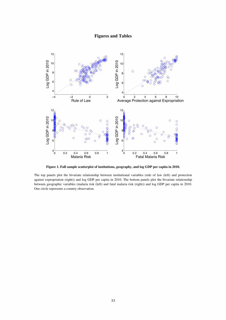
33

Figures and Tables

Figure 1. Full sample scatterplot of institutions, geography, and log GDP per capita in 2010.

The top panels plot the bivariate relationship between institutional variables (rule of law (left) and protection

against expropriation (right)) and log GDP per capita in 2010. The bottom panels plot the bivariate relationship

between geographic variables (malaria risk (left) and fatal malaria risk (right)) and log GDP per capita in 2010.

One circle represents a country observation.

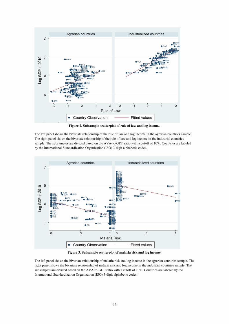
34

Figure 2. Subsample scatterplot of rule of law and log income.

The left panel shows the bivariate relationship of the rule of law and log income in the agrarian countries sample.

The right panel shows the bivariate relationship of the rule of law and log income in the industrial countries

sample. The subsamples are divided based on the AVA-to-GDP ratio with a cutoff of 10%. Countries are labeled

by the International Standardization Organization (ISO) 3-digit alphabetic codes.

Figure 3. Subsample scatterplot of malaria risk and log income.

The left panel shows the bivariate relationship of malaria risk and log income in the agrarian countries sample. The

right panel shows the bivariate relationship of malaria risk and log income in the industrial countries sample. The

subsamples are divided based on the AVA-to-GDP ratio with a cutoff of 10%. Countries are labeled by the

International Standardization Organization (ISO) 3-digit alphabetic codes.

AFG

ALBARM

AZE

BGD

BLR

BLZ

BEN

BTNBOL

BIH

BGR

BFA

BDI

KHM

CMR

CAF

TCD

CHN

COL

COG

ZAR

CRI

CIV

DOMECU

EGYSLV

GNQ

ERIETH

GMB

GEO

GHA

GTM

GINGNB

GUY

HTI

HND

IND

IDN

IRN

IRQ

KAZ

KENKGZ

LAO

LBN

LSO

LBR

MKD

MDGMWI

MYS

MLI

MRT

MNGMAR

MOZ

NAM

NPL

NIC

NER

NGA

PAK

PNG

PRY

PHL

ROM

RWA

SEN

SLE

LKA

SDN

SUR

SWZSYR

TJK

TZA

THA

TGO

TUN

TUR

UGA

UKR

UZB VNMYEMZMB

ZWE

DZA AGO

ARG

AUSAUTBEL

BWA

BRA

BRN

CAN

CHLHRV

CUB

CYP

CZE

DNK

EST

FINFRA

GAB

DEU

GRC

HUN

ISLIRL

ISRITA

JAM

JPN

JOR

KOR

KWT

LVALTU

LUX

MUSMEX

NLD

NZL

NOR

OMN

PAN

PER

POL

PRT

QAT

SAU

SGP

SVK

SVN

ZAF

ESP

SWE

CHE

TTO

AREGBR

USA

URYVEN

68

10

12

0 .5 1 0 .5 1

Agrarian countries Industrialized countries

Country Observation Fitted values

Log G

DP

in 2

010

Malaria Risk

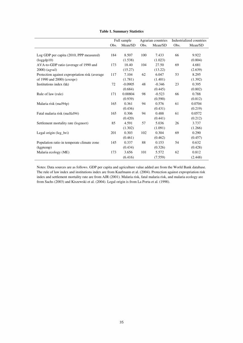
35

Table 1. Summary Statistics

Full sample Agrarian countries Industrialized countries

Obs. Mean/SD Obs. Mean/SD Obs. Mean/SD

Log GDP per capita (2010, PPP measured)

(loggdp10)

184 8.507 100 7.433 66 9.922

(1.538) (1.023) (0.804)

AVA-to-GDP ratio (average of 1990 and

2000) (agval)

173 18.40 104 27.50 69 4.681

(15.27) (13.22) (2.639)

Protection against expropriation risk (average

of 1990 and 2000) (avexpr)

117 7.104 62 6.047 53 8.295

(1.781) (1.401) (1.392)

Institutions index (kk) 72 -0.0905 48 -0.346 23 0.395

(0.684) (0.445) (0.802)

Rule of law (rule) 171 0.00804 98 -0.523 66 0.788

(0.939) (0.590) (0.812)

Malaria risk (mal94p) 165 0.361 94 0.576 61 0.0704

(0.436) (0.431) (0.219)

Fatal malaria risk (malfal94) 165 0.306 94 0.488 61 0.0572

(0.420) (0.441) (0.212)

Settlement mortality rate (logmort) 85 4.591 57 5.036 26 3.737

(1.302) (1.091) (1.266)

Legal origin (leg_bri) 201 0.303 102 0.304 69 0.290

(0.461) (0.462) (0.457)

Population ratio in temperate climate zone

(kgptemp)

145 0.337 88 0.153 54 0.632

(0.434) (0.326) (0.428)

Malaria ecology (ME) 173 3.656 101 5.572 62 0.812

(6.416) (7.559) (2.448)

Notes: Data sources are as follows. GDP per capita and agriculture value added are from the World Bank database.

The rule of law index and institutions index are from Kaufmann et al. (2004). Protection against expropriation risk

index and settlement mortality rate are from AJR (2001). Malaria risk, fatal malaria risk, and malaria ecology are

from Sachs (2003) and Kiszewski et al. (2004). Legal origin is from La Porta et al. (1998).

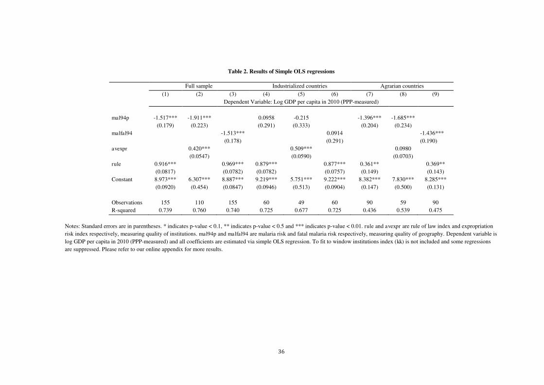
36

Table 2. Results of Simple OLS regressions

Full sample Industrialized countries Agrarian countries

(1) (2) (3) (4) (5) (6) (7) (8) (9)

Dependent Variable: Log GDP per capita in 2010 (PPP-measured)

mal94p -1.517*** -1.911*** 0.0958 -0.215 -1.396*** -1.685***

(0.179) (0.223) (0.291) (0.333) (0.204) (0.234)

malfal94 -1.513*** 0.0914 -1.436***

(0.178) (0.291) (0.190)

avexpr 0.420*** 0.509*** 0.0980

(0.0547) (0.0590) (0.0703)

rule 0.916*** 0.969*** 0.879*** 0.877*** 0.361** 0.369**

(0.0817) (0.0782) (0.0782) (0.0757) (0.149) (0.143)

Constant 8.973*** 6.307*** 8.887*** 9.219*** 5.751*** 9.222*** 8.382*** 7.830*** 8.285***

(0.0920) (0.454) (0.0847) (0.0946) (0.513) (0.0904) (0.147) (0.500) (0.131)

Observations 155 110 155 60 49 60 90 59 90

R-squared 0.739 0.760 0.740 0.725 0.677 0.725 0.436 0.539 0.475

Notes: Standard errors are in parentheses. * indicates p-value < 0.1, ** indicates p-value < 0.5 and *** indicates p-value < 0.01. rule and avexpr are rule of law index and expropriation

risk index respectively, measuring quality of institutions. mal94p and malfal94 are malaria risk and fatal malaria risk respectively, measuring quality of geography. Dependent variable is

log GDP per capita in 2010 (PPP-measured) and all coefficients are estimated via simple OLS regression. To fit to window institutions index (kk) is not included and some regressions

are suppressed. Please refer to our online appendix for more results.

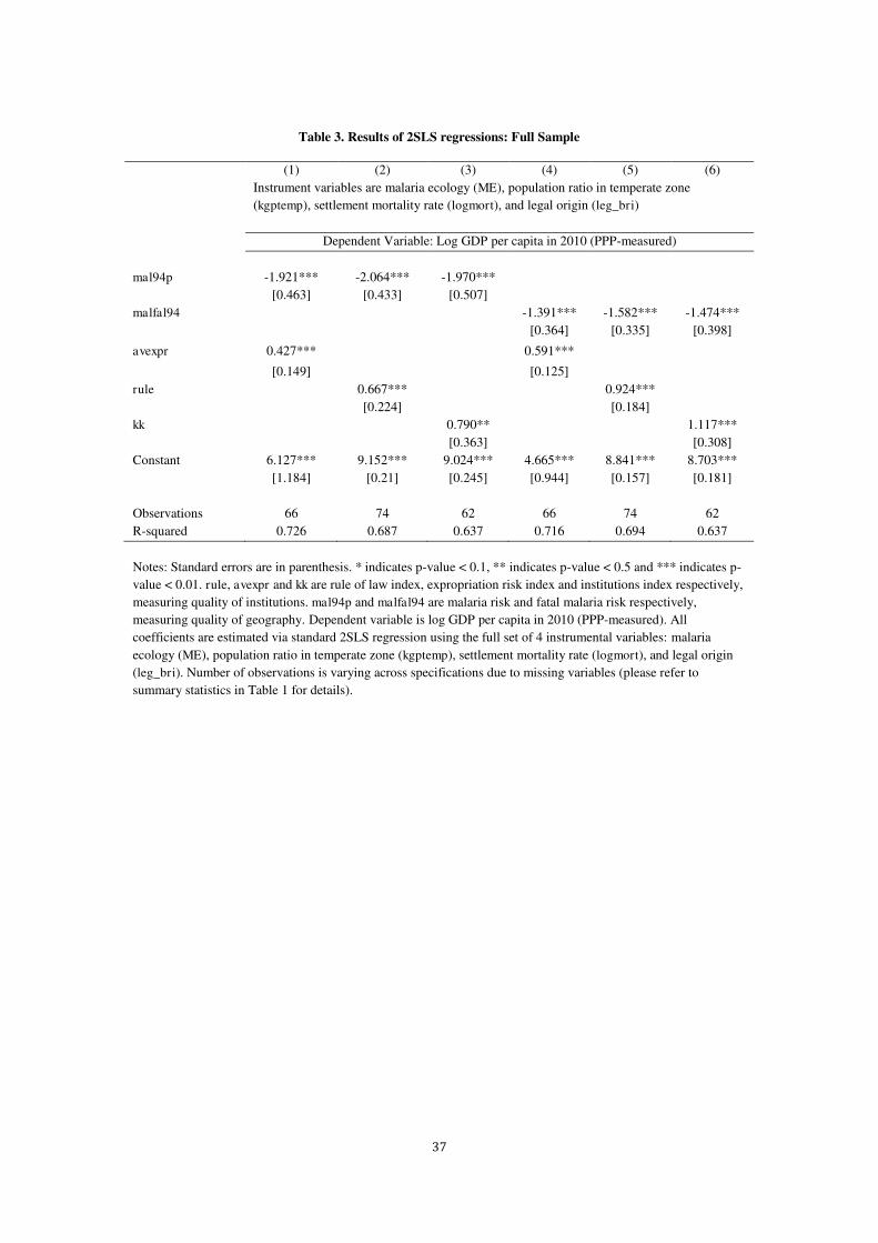
37

Table 3. Results of 2SLS regressions: Full Sample

(1) (2) (3) (4) (5) (6)

Instrument variables are malaria ecology (ME), population ratio in temperate zone

(kgptemp), settlement mortality rate (logmort), and legal origin (leg_bri)


mal94p -1.921*** -2.064*** -1.970***

[0.463] [0.433] [0.507]

malfal94 -1.391*** -1.582*** -1.474***

[0.364] [0.335] [0.398]

avexpr 0.427*** 0.591*** [0.149] [0.125]

rule 0.667*** 0.924***

[0.224] [0.184]

kk 0.790** 1.117***

[0.363] [0.308]

Constant 6.127*** 9.152*** 9.024*** 4.665*** 8.841*** 8.703***

[1.184] [0.21] [0.245] [0.944] [0.157] [0.181]

Observations 66 74 62 66 74 62

R-squared 0.726 0.687 0.637 0.716 0.694 0.637

Notes: Standard errors are in parenthesis. * indicates p-value < 0.1, ** indicates p-value < 0.5 and *** indicates p-

value < 0.01. rule, avexpr and kk are rule of law index, expropriation risk index and institutions index respectively,

measuring quality of institutions. mal94p and malfal94 are malaria risk and fatal malaria risk respectively,

measuring quality of geography. Dependent variable is log GDP per capita in 2010 (PPP-measured). All

coefficients are estimated via standard 2SLS regression using the full set of 4 instrumental variables: malaria

ecology (ME), population ratio in temperate zone (kgptemp), settlement mortality rate (logmort), and legal origin

(leg_bri). Number of observations is varying across specifications due to missing variables (please refer to

summary statistics in Table 1 for details).

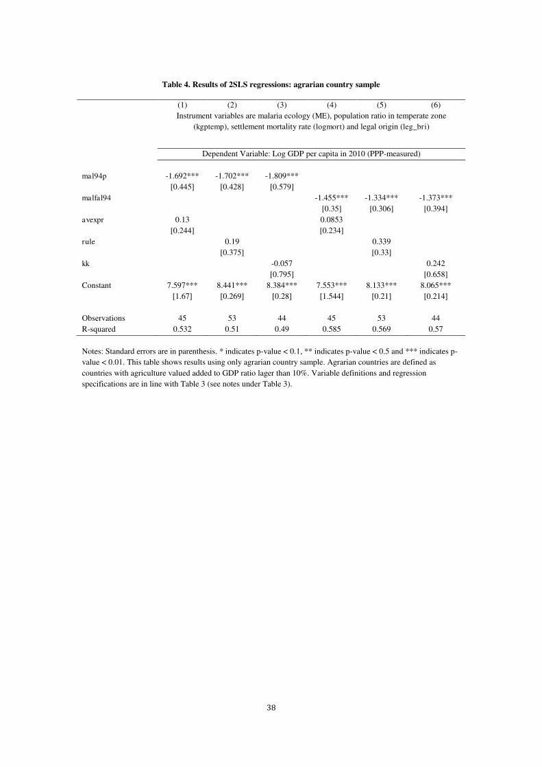
38

Table 4. Results of 2SLS regressions: agrarian country sample

(1) (2) (3) (4) (5) (6)


(kgptemp), settlement mortality rate (logmort) and legal origin (leg_bri)


mal94p -1.692*** -1.702*** -1.809***

[0.445] [0.428] [0.579]

malfal94 -1.455*** -1.334*** -1.373***

[0.35] [0.306] [0.394]

avexpr 0.13 0.0853

[0.244] [0.234]

rule 0.19 0.339

[0.375] [0.33]

kk -0.057 0.242

[0.795] [0.658]

Constant 7.597*** 8.441*** 8.384*** 7.553*** 8.133*** 8.065***

[1.67] [0.269] [0.28] [1.544] [0.21] [0.214]


R-squared 0.532 0.51 0.49 0.585 0.569 0.57


value < 0.01. This table shows results using only agrarian country sample. Agrarian countries are defined as

countries with agriculture valued added to GDP ratio lager than 10%. Variable definitions and regression

specifications are in line with Table 3 (see notes under Table 3).

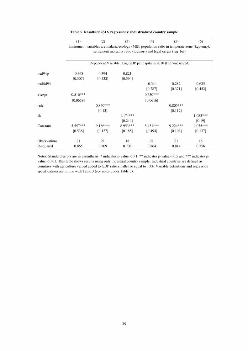
39

Table 5. Results of 2SLS regressions: industrialized country sample

(1) (2) (3) (4) (5) (6)

Instrument variables are malaria ecology (ME), population ratio in temperate zone (kgptemp),

settlement mortality ratio (logmort) and legal origin (leg_bri)


mal94p -0.368 0.394 0.821

[0.307] [0.432] [0.594]

malfal94 -0.344 0.282 0.625

[0.287] [0.371] [0.452]

avexpr 0.516*** 0.530*** [0.0659] [0.0616]

rule 0.840*** 0.805***

[0.13] [0.112]

kk 1.174*** 1.083***

[0.244] [0.19]

Constant 5.557*** 9.186*** 8.953*** 5.431*** 9.224*** 9.035***

[0.538] [0.127] [0.185] [0.494] [0.106] [0.137]


R-squared 0.865 0.809 0.708 0.864 0.814 0.756


value < 0.01. This table shows results using only industrial country sample. Industrial countries are defined as

countries with agriculture valued added to GDP ratio smaller or equal to 10%. Variable definitions and regression

specifications are in line with Table 3 (see notes under Table 3).

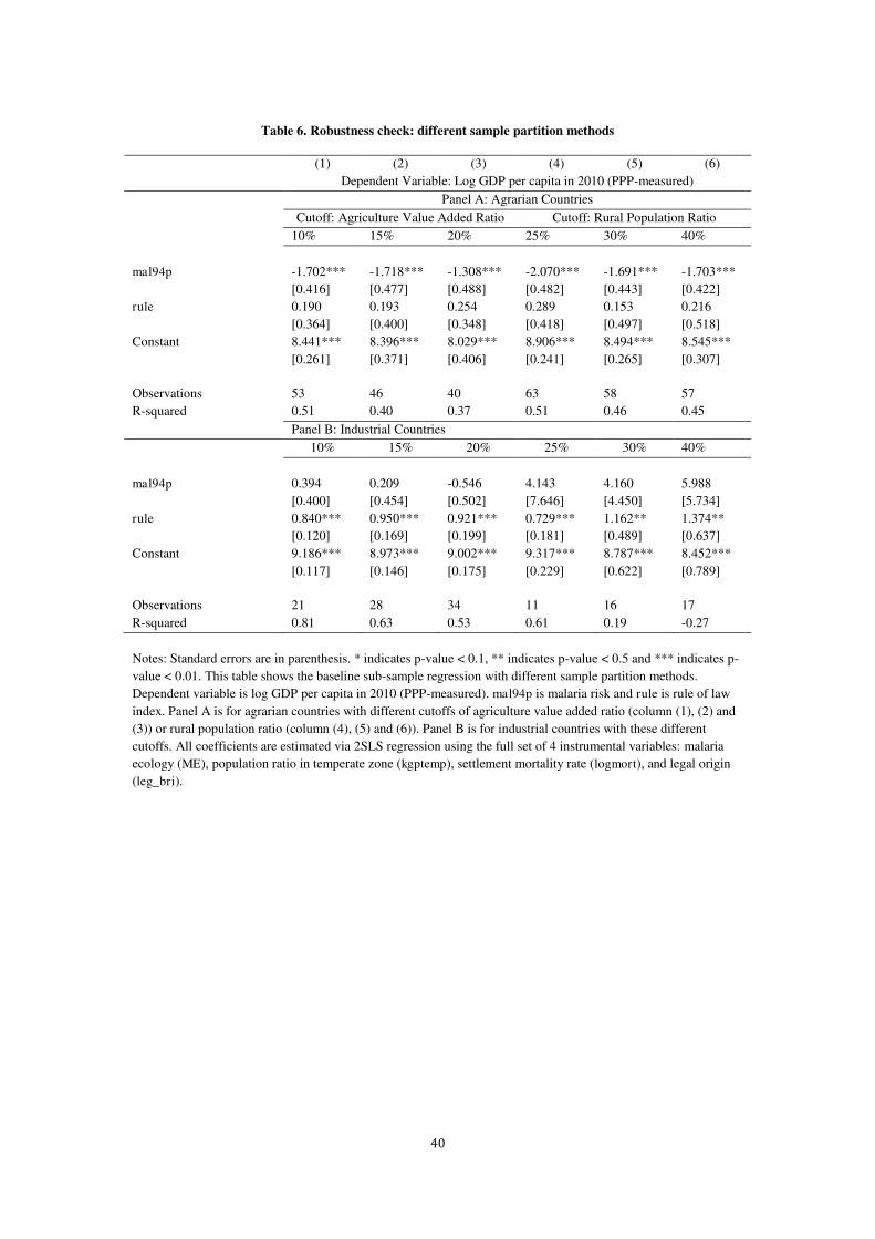
40

Table 6. Robustness check: different sample partition methods

(1) (2) (3) (4) (5) (6)


Panel A: Agrarian Countries

Cutoff: Agriculture Value Added Ratio Cutoff: Rural Population Ratio

10% 15% 20% 25% 30% 40%

mal94p -1.702*** -1.718*** -1.308*** -2.070*** -1.691*** -1.703***

[0.416] [0.477] [0.488] [0.482] [0.443] [0.422]

rule 0.190 0.193 0.254 0.289 0.153 0.216

[0.364] [0.400] [0.348] [0.418] [0.497] [0.518]

Constant 8.441*** 8.396*** 8.029*** 8.906*** 8.494*** 8.545***

[0.261] [0.371] [0.406] [0.241] [0.265] [0.307]


R-squared 0.51 0.40 0.37 0.51 0.46 0.45

Panel B: Industrial Countries

10% 15% 20% 25% 30% 40%

mal94p 0.394 0.209 -0.546 4.143 4.160 5.988

[0.400] [0.454] [0.502] [7.646] [4.450] [5.734]

rule 0.840*** 0.950*** 0.921*** 0.729*** 1.162** 1.374**

[0.120] [0.169] [0.199] [0.181] [0.489] [0.637]

Constant 9.186*** 8.973*** 9.002*** 9.317*** 8.787*** 8.452***

[0.117] [0.146] [0.175] [0.229] [0.622] [0.789]


R-squared 0.81 0.63 0.53 0.61 0.19 -0.27


value < 0.01. This table shows the baseline sub-sample regression with different sample partition methods.

Dependent variable is log GDP per capita in 2010 (PPP-measured). mal94p is malaria risk and rule is rule of law

index. Panel A is for agrarian countries with different cutoffs of agriculture value added ratio (column (1), (2) and

(3)) or rural population ratio (column (4), (5) and (6)). Panel B is for industrial countries with these different

cutoffs. All coefficients are estimated via 2SLS regression using the full set of 4 instrumental variables: malaria

ecology (ME), population ratio in temperate zone (kgptemp), settlement mortality rate (logmort), and legal origin

(leg_bri).

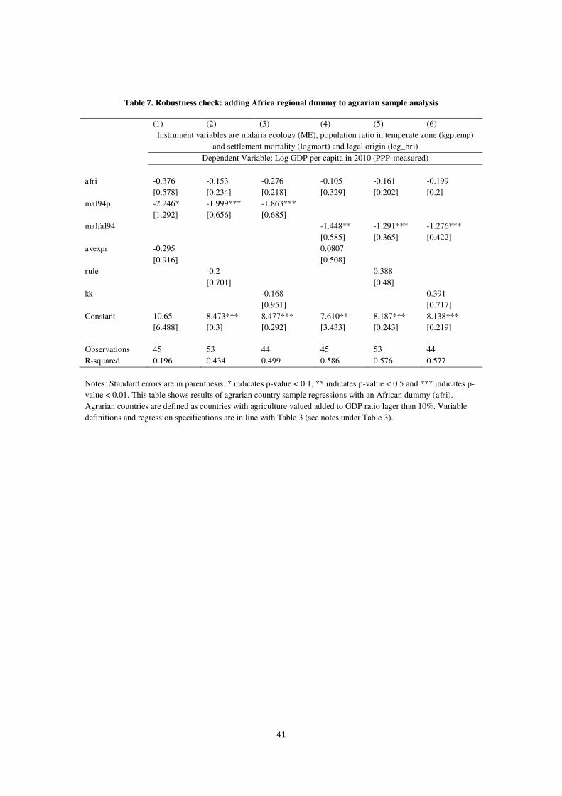
41

Table 7. Robustness check: adding Africa regional dummy to agrarian sample analysis

(1) (2) (3) (4) (5) (6)

Instrument variables are malaria ecology (ME), population ratio in temperate zone (kgptemp)

and settlement mortality (logmort) and legal origin (leg_bri)


afri -0.376 -0.153 -0.276 -0.105 -0.161 -0.199

[0.578] [0.234] [0.218] [0.329] [0.202] [0.2]

mal94p -2.246* -1.999*** -1.863***

[1.292] [0.656] [0.685]

malfal94 -1.448** -1.291*** -1.276***

[0.585] [0.365] [0.422]

avexpr -0.295 0.0807

[0.916] [0.508]

rule -0.2 0.388

[0.701] [0.48]

kk -0.168 0.391

[0.951] [0.717]

Constant 10.65 8.473*** 8.477*** 7.610** 8.187*** 8.138***

[6.488] [0.3] [0.292] [3.433] [0.243] [0.219]


R-squared 0.196 0.434 0.499 0.586 0.576 0.577


value < 0.01. This table shows results of agrarian country sample regressions with an African dummy (afri).

Agrarian countries are defined as countries with agriculture valued added to GDP ratio lager than 10%. Variable

definitions and regression specifications are in line with Table 3 (see notes under Table 3).

42

Table 8. Robustness check: additional controls

(1) (2) (3) (4) (5) (6) (7) (8)

Control for log

openness

Control for log

openness, along with

its instrument of Frankel

and Romer (1999)

Control for share

of the national

population living within

100km of the coast

Control for British

colony

Control for British

and French colony

Control for major

oil producer

Control for years

of schooling

in population

above aged 25

Control for

Protestants as % of

population

Panel A: Full Sample. Dependent Variable: Log GDP Per Capita 2010 (PPP-measured)

rule 0.688*** 0.652*** 0.687*** 0.753*** 0.776*** 0.589*** 0.160 0.585**

(0.238) (0.242) (0.221) (0.221) (0.227) (0.208) (0.286) (0.237) mal94p -2.132*** -2.043*** -1.957*** -1.935*** -1.794*** -2.144*** -1.608*** -2.170***

(0.462) (0.481) (0.459) (0.417) (0.478) (0.411) (0.474) (0.445) lcopen 0.315 -0.144

(0.202) (0.320) pop100km 0.251

(0.317) coluk -0.132 -0.233

(0.217) (0.248) colfr -0.251

(0.275) oil 0.919**

(0.375) tyr60 0.264**

(0.119) prot 0.00676

(0.00721) Constant 8.004*** 9.682*** 8.987*** 9.148*** 9.179*** 9.108*** 7.830*** 9.118***

(0.754) (1.157) (0.312) (0.210) (0.205) (0.209) (0.689) (0.214)

Observations 73 73 74 74 74 74 52 74 R-squared 0.686 0.672 0.695 0.687 0.697 0.714 0.882 0.690

Panel B: Agrarian Country Sample. Dependent Variable: Log GDP Per Capita 2010 (PPP-measured)

rule 0.264 0.143 0.243 0.400 0.490 0.0800 0.245 0.201

(0.390) (0.417) (0.341) (0.321) (0.313) (0.354) (0.230) (0.376) mal94p -1.804*** -1.751*** -1.416*** -1.523*** -1.360*** -1.892*** -1.315** -1.655***

(0.460) (0.489) (0.408) (0.398) (0.434) (0.409) (0.541) (0.449) lcopen 0.453** -0.0429

(0.220) (0.376) pop100km 0.683**

(0.311) coluk -0.0372 -0.152

(0.210) (0.259) colfr -0.206

(0.265) oil 0.756

(0.713) tyr60 0.297**

(0.120) prot -0.00329

(0.00829) Constant 6.845*** 8.626*** 7.999*** 8.447*** 8.489*** 8.497*** 7.559*** 8.437***

(0.855) (1.368) (0.359) (0.276) (0.284) (0.275) (0.642) (0.271)


Panel C: Industrial Country Sample. Dependent Variable: Log GDP Per Capita 2010 (PPP-measured)

rule 0.838*** 0.837*** 0.833*** 0.849*** 0.838*** 0.859*** 1.405 0.878***

(0.132) (0.133) (0.134) (0.145) (0.135) (0.128) (0.977) (0.144) mal94p 0.484 0.510 0.334 0.376 0.366 0.412 2.732 0.453

(0.456) (0.448) (0.461) (0.444) (0.440) (0.409) (3.110) (0.456) lcopen -0.127 -0.168

(0.165) (0.182)

43

pop100km -0.135 (0.313)

coluk -0.0333 -0.0304 (0.213) (0.218)

colfr -0.0366 (0.343)

oil 0.371 (0.220)

tyr60 -0.158 (0.305)

prot -0.00358 (0.00575)

Constant 9.648*** 9.798*** 9.278*** 9.197*** 9.205*** 9.107*** 9.822*** 9.222*** (0.614) (0.686) (0.249) (0.142) (0.142) (0.134) (1.409) (0.143)


Panel D: Full Sample. Dependent Variable: AVA-to-GDP ratio in 1990-2000.

rule -1.489 -1.068 -2.635 -4.767* -4.988* -1.684 3.984 -1.343

(2.845) (2.979) (2.755) (2.723) (2.856) (2.702) (4.718) (3.039) mal94p 26.84*** 25.31*** 21.11*** 19.94*** 20.19*** 24.21*** 23.68*** 24.90***

(5.557) (5.973) (5.748) (5.222) (6.118) (5.379) (7.873) (5.721) lcopen -5.457** 1.516

(2.390) (3.914) pop100km -6.102

(3.977) coluk 3.632 3.024

(2.629) (3.072) colfr -1.725

(3.483) oil -8.203*

(4.916) tyr60 -2.771

(1.970) prot -0.0733

(0.0927) Constant 27.81*** 2.449 13.08*** 9.162*** 9.616*** 9.490*** 21.76* 9.373***

(8.895) (14.06) (3.903) (2.628) (2.603) (2.727) (11.45) (2.750)



value < 0.01. This table shows baseline regression results with various control variables. Panel A, B, and C show

regressions results with log GDP Per Capita 2010 (PPP-measured) as dependent variable, and Panel D show

regressions results with agriculture value added as dependent variable. All coefficients are estimated via 2SLS

regression using the full set of 4 instrumental variables: malaria ecology (ME), population ratio in temperate zone

(kgptemp), settlement mortality rate (logmort), and legal origin (leg_bri).

44

Table 9. OLS regression results on industrialization

(1) (2) (3) (4) (5) (6)

Panel A: Dependent Variable: AVA-to-GDP Ratio

mal94p 16.93*** 14.76*** 18.14***

[2.542] [2.293] [3.288]

malfal94 16.82*** 14.87*** 18.10***

[2.436] [2.254] [3.179]

avexpr -2.740*** -3.081***

[0.613] [0.573]

rule -6.980*** -7.436***

[1.051] [1.003]

kk -3.483 -3.640*

[2.191] [2.135]

Constant 29.62*** 13.14*** 10.93*** 33.08*** 13.92*** 12.56***

[5.072] [1.187] [1.946] [4.615] [1.088] [1.684]

Observations 111 154 67 111 154 67

R-squared 0.59 0.56 0.52 0.60 0.57 0.53

Panel B: Dependent Variable: Rural Population Ratio

mal94p 35.66*** 27.38*** 26.67***

[4.044] [3.320] [5.119]

malfal94 33.27*** 26.34*** 25.01***

[4.028] [3.349] [5.106]

avexpr -2.100** -3.099***

[0.968] [0.937]

rule -8.005*** -9.093***

[1.509] [1.474]

kk -10.97*** -11.86***

[3.390] [3.397]

Constant 46.62*** 37.79*** 37.06*** 56.59*** 39.60*** 40.09***

[8.016] [1.699] [3.010] [7.557] [1.596] [2.680]

Observations 111 155 66 111 155 66

R-squared 0.61 0.57 0.58 0.59 0.55 0.56


value < 0.01. This table shows regression results when degree of industrialization is dependent variable. In Panel A

the proxy of industrialization is value added to GDP ratio while in Panel B the proxy is rural population ratio. All

coefficients are estimated via OLS regressions.

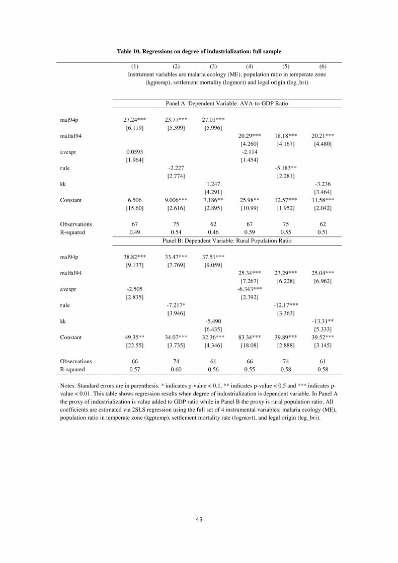
45

Table 10. Regressions on degree of industrialization: full sample

(1) (2) (3) (4) (5) (6)


(kgptemp), settlement mortality (logmort) and legal origin (leg_bri)

Panel A: Dependent Variable: AVA-to-GDP Ratio

mal94p 27.24*** 23.77*** 27.01***

[6.119] [5.399] [5.996]

malfal94 20.29*** 18.18*** 20.21***

[4.260] [4.167] [4.480]

avexpr 0.0593 -2.114

[1.964] [1.454]

rule -2.227 -5.183**

[2.774] [2.281]

kk 1.247 -3.236

[4.291] [3.464]

Constant 6.506 9.006*** 7.186** 25.98** 12.57*** 11.58***

[15.60] [2.616] [2.895] [10.99] [1.952] [2.042]


R-squared 0.49 0.54 0.46 0.59 0.55 0.51

Panel B: Dependent Variable: Rural Population Ratio

mal94p 38.82*** 33.47*** 37.51***

[9.137] [7.769] [9.059]

malfal94 25.34*** 23.29*** 25.04***

[7.267] [6.228] [6.962]

avexpr -2.505 -6.343***

[2.835] [2.392]

rule -7.217* -12.17***

[3.946] [3.363]

kk -5.490 -13.31**

[6.435] [5.333]

Constant 49.35** 34.07*** 32.36*** 83.34*** 39.89*** 39.52***

[22.55] [3.735] [4.346] [18.08] [2.888] [3.145]


R-squared 0.57 0.60 0.56 0.55 0.58 0.58


value < 0.01. This table shows regression results when degree of industrialization is dependent variable. In Panel A

the proxy of industrialization is value added to GDP ratio while in Panel B the proxy is rural population ratio. All

coefficients are estimated via 2SLS regression using the full set of 4 instrumental variables: malaria ecology (ME),

population ratio in temperate zone (kgptemp), settlement mortality rate (logmort), and legal origin (leg_bri).

RESEARCH DIVISION · 2019-01-02 · Institutions Do Not Rule: Reassessing the Driving Forces of...

Documents

Transcript of RESEARCH DIVISION · 2019-01-02 · Institutions Do Not Rule: Reassessing the Driving Forces of...