Research Discussion Paper

The Sticky Information Phillips Curve: Evidence for Australia

Christian Gillitzer

RDP 2015-04

The contents of this publication shall not be reproduced, sold or distributed without the prior consent of the Reserve Bank of Australia and, where applicable, the prior consent of the external source concerned. Requests for consent should be sent to the Head of Information Department at the email address shown above.

ISSN 1448-5109 (Online)

The Discussion Paper series is intended to make the results of the current economic research within the Reserve Bank available to other economists. Its aim is to present preliminary results of research so as to encourage discussion and comment. Views expressed in this paper are those of the authors and not necessarily those of the Reserve Bank. Use of any results from this paper should clearly attribute the work to the authors and not to the Reserve Bank of Australia.

Enquiries:

Phone: +61 2 9551 9830 Facsimile: +61 2 9551 8033 Email: rbainfo@rba.gov.au Website: http://www.rba.gov.au

The Sticky Information Phillips Curve: Evidence forAustralia

Christian Gillitzer

Research Discussion Paper2015-04

April 2015

Economic Research DepartmentReserve Bank of Australia

The views expressed in this paper are those of the author and do not necessarilyreflect the views of the Reserve Bank of Australia. I would like to thankJames Hansen, Christopher Kent, Adrian Pagan, Michael Plumb, Daniel Rees andJohn Simon for helpful comments. The author is solely responsible for any errors.

Author: gillitzerc at domain rba.gov.au

Media Office: rbainfo@rba.gov.au

Abstract

The Sticky Information Phillips Curve (SIPC) provides a theoretically appealingalternative to the sticky-price New-Keynesian Phillips curve (NKPC). This paperassesses the empirical performance of the SIPC for Australia. There is only weakevidence in favour of the SIPC over the low-inflation period. Parameter estimatesare sensitive to inflation measures and sample periods, and are theoreticallyinconsistent for several specifications. The apparent poor performance of the SIPCin part reflects the fact that inflation has become difficult to model since theintroduction of inflation targeting. Over sample periods including the early 1990sdisinflation, the SIPC appears to fit the data better.

JEL Classification Numbers: E3, E31Keywords: sticky information, Phillips curve, inflation, Australia

i

Table of Contents

1. Introduction 1

2. Model and Estimation 4

2.1 Sticky Information Phillips Curve 4

2.2 New-Keynesian Phillips Curve 6

3. Forecasts 8

3.1 Availability and Construction 8

3.2 Forecast Performance 11

4. Results 14

4.1 Low-inflation Period 14

4.2 Long Sample 17

4.3 Comparing the SIPC and the NKPC 20

4.4 Adaptive Expectations Phillips Curve 23

5. Conclusion 25

Appendix A: Confidence Intervals for Econometric Forecasts 27

Appendix B: SIPC Estimates for 1980–1990 29

References 30

ii

The Sticky Information Phillips Curve: Evidence for Australia

Christian Gillitzer

1. Introduction

Modelling inflation is a core task for inflation-targeting central banks. Like othercentral banks, the Reserve Bank of Australia (RBA) evaluates and uses a varietyof models for inflation. The set of models differ substantially in their style andpurpose. At one end of the spectrum are reduced-form single or multi-equationmodels. These models typically impose few parameter restrictions and are used forforecasting. At the other end of the spectrum are microfounded dynamic stochasticgeneral equilibrium (DSGE) models, which are mostly used for scenario analysis.In between these two extremes are more microfounded single-equation models.While reduced-form models typically provide the best forecasting performance,their lack of structure makes them less suited to policy analysis.

The New-Keynesian Phillips curve (NKPC) has become the canonicalmicrofounded model of inflation in the academic community, being widely usedin theoretical work. In its pure or hybrid variants, it is also a central elementof DSGE models used by most central banks (e.g. Smets and Wouters 2007).Like all models, its usefulness for policy analysis depends on the assumptionsunderpinning the model. The key assumption of the New-Keynesian sticky-pricemodel is a restriction on the frequency with which firms can change their prices.This assumption is consistent with the infrequency with which retail prices changefor many goods and services. But a large literature highlights the inability ofthe basic sticky-price model to match the inertial behaviour of inflation, andthe delayed and gradual response of inflation to monetary policy shocks.1 Othercounterfactual predictions of the sticky-price model are the possibilities of costlessdisinflations and disinflationary booms (Ball 1994).

The New-Keynesian model has trouble matching the inertial behaviour of inflationbecause it implies that, while the price level is sticky, the inflation rate can jump.

1 See Mankiw (2001), and the references therein, for a critique of the sticky-price model, andChristiano, Eichenbaum and Evans (1999) for evidence on the response of inflation to monetarypolicy shocks.

2

The model assumes that a randomly chosen subset of firms are able to change theirprice each period. Firms anticipate the likelihood of being stuck at their reset pricefor several periods, making inflation highly forward-looking and responsive tomacroeconomic news. The peak response of inflation to a monetary policy shockin the canonical sticky-price NKPC is immediate, and thus the NKPC cannotmatch the persistence of inflation, or generate the output-inflation correlationsevident in the data (Fuhrer and Moore 1995; Mankiw 2001).

As an alternative to the sticky-price model, Mankiw and Reis (2002) proposea Sticky Information Phillips Curve (SIPC). Building on Lucas (1973) andCarroll (2003), the SIPC assumes that macroeconomic news disseminates slowlythroughout the population. Only some firms receive updated information aboutoutput and inflation each period, with the remainder continuing to set pricesbased on outdated information. Firms are always free to change prices, but onlysome firms change prices based on updated information. Slow dissemination ofmacroeconomic news generates inertial inflation dynamics when there is strategiccomplementarity in price setting. Firms acquiring new information take intoaccount that other firms remain uninformed, and incorporate macroeconomic newsinto pricing decisions gradually, as the share of informed firms rises. In contrast,inflation in the NKPC model is entirely forward looking.

This paper provides the first estimates of the SIPC for Australian data. Themodel is tested using a range of inflation measures, forecast series and sampleperiods. Overall, the estimation results provide only weak support for the SIPC,particularly over the low-inflation period. The estimated degree of informationrigidity differs substantially across sample periods and inflation measures. Forconsumer price index (CPI) inflation over the 1995–2013 period, the estimateddegree of information rigidity using Consensus Economics and official RBAforecasts is theoretically inconsistent, indicating rejection of the model. But forunderlying inflation, the estimated degree of information rigidity is theoreticallyconsistent, with estimates implying that firms on average update their informationsets each 6–8 quarters. Including data prior to the introduction of inflationtargeting in the estimation sample improves the performance of the SIPC, but thereis still substantial parameter instability across specifications.

Some of the estimated parameter instability can be explained by differences ininflation inertia across sample periods and inflation measures. A high degree of

3

information rigidity puts substantial weight on old forecasts of current inflation,generating sluggish inflation dynamics. This is a key objective of the sticky-information model, but it is inconsistent with the behaviour of CPI inflationover the low-inflation period. Conversely, the variability of the inertial trendcomponent of inflation was relatively high prior to the introduction of inflationtargeting (IT), and the estimated degree of information rigidity is, in general,substantial. Reflecting this, the fit of the SIPC is generally better over sampleperiods including the pre-IT regime.

Reflecting the weak relationship between inflation and the output gap, particularlyover the low-inflation period, the estimated degree of real rigidity is impreciselyestimated. The relationship between the nominal and real side of the modeldepends non-linearly on the degree of information rigidity, and the degree of realrigidity is most imprecisely estimated when the degree of information rigidity ishigh.

An important theoretical feature of the SIPC is its ability to generate costlydisinflations. Despite this, the SIPC does not perform well during the early 1990sdisinflation, except with very low levels of information rigidity. This is becausethe SIPC places weight on dated real-time long-horizon inflation forecasts,which substantially overpredicted inflation during the early 1990s disinflation.Coibion (2010) labels this the real-time forecast error effect. In contrast, theforward-looking NKPC model better predicts the disinflation because it placesno weight on dated long-horizon inflation forecasts.

These findings are broadly similar to Coibion (2010) for US data, who findsthat the SIPC generates excessively inertial inflation dynamics, and can bestrongly rejected in favour of the NKPC. Kahn and Zhu (2006) present morefavourable evidence for the SIPC using US data, estimating that firms updatetheir information sets each 3–7 quarters. Dopke et al (2008) provide similarlyfavourable evidence for France, Germany and the United Kingdom, findingthat firms update their information sets once a year. However, both Kahn andZhu (2006) and Dopke et al (2008) impose the degree of real rigidity, rather thanestimating the parameter. I find that imposing the degree of real rigidity can havea substantial effect on the estimated degree of information rigidity. Kiley (2007)and Koronek (2008) both reject the SIPC in favour of the NKPC using US data,although Kiley finds that a hybrid NKPC model fits the data best, and suggests

4

that the importance of lagged inflation may capture information rigidity. However,both Kiley (2007) and Koronek (2008) use in-sample forecasts, which can bemisleading, particularly when there are mean-shifts in inflation. I use only real-time or quasi real-time forecasts in assessing the empirical performance of theSIPC. More broadly, this paper’s findings add to a body of work modellingAustralian inflation. Norman and Richards (2010) provide a recent criticalevaluation of structural and reduced-form single-equation inflation models forAustralia. Their main finding is that an expectations-augmented standard Phillipscurve and mark-up models outperform the NKPC in terms of in-sample fit andsignificance of the model coefficients. Given that I find the fit of the SIPC to begenerally no better than the NKPC, the ranking of models in Norman and Richardsis unchanged.

The remainder of the paper proceeds as follows: Section 2 describes the SIPC andNKPC models, and discusses estimation issues; Section 3 describes the forecastsused; and Section 4 presents the estimation results. Some concluding thoughts areoffered in Section 5.

2. Model and Estimation

2.1 Sticky Information Phillips Curve

The log of a firm’s desired price p∗t , relative to the log aggregate price level pt , isproportional to the output gap:

p∗t = pt +αxt , (1)

where xt is the output gap and α is the degree of real rigidity (the elasticity ofa firm’s desired relative price with respect to the output gap). The smaller is theparameter α , the greater is the degree of strategic complementarity between firms,reducing the sensitivity of firms’ desired price to the output gap.2 Each period,a randomly chosen fraction (1−λ ) of firms receive updated inflation and outputgap forecasts for each quarter in the future.3 The remaining λ share of firms do not

2 This condition can be derived from a firm’s profit maximisation condition. See, for example,Blanchard and Kiyotaki (1987).

3 The SIPC assumes that λ is a structural parameter. See Reis (2006) for a model thatmicrofounds the optimal degree of inattention.

5

acquire new information, and continue to set prices based on outdated information.The assumption that a fraction of firms continue to work with outdated informationeach period enables the SIPC to generate inertial inflation dynamics: only pricesset by firms acquiring new information will reflect shocks to inflation and outputgap forecasts. Combining Equation (1) with the assumption of a state-independentprobability of acquiring new forecasts yields the SIPC:

πt =

[1−λ

λ

]αxt +(1−λ )

∞∑j=0

λjEt− j−1 [πt +α∆xt ] , (2)

where πt is the quarterly inflation rate and ∆xt = xt −xt−1 is the contemporaneouschange in the output gap. Equation (2) indicates that current inflation in partreflects past expectations of current inflation. Mankiw and Reis (2002) motivatethe SIPC by relation to a contracting model, in which prices reflect expectationsat the time contracts were set. When firms acquire new information, they areassumed to receive rational expectations forecasts. With this assumption, themodel resembles Carroll’s (2003) epidemic model of information diffusion,in which a random subset of consumers come into contact with professionalforecasters each period.

Reflecting the fact that Australia is a small open economy, the baseline closed-economy SIPC is augmented with an import price term, allowing firms’ desiredprice to depend on both the output gap and the cost of imported goods andservices. With import prices, Equation (1) generalises to p∗t = pt +αxt + ξ π

mt ,

where πmt ≡ pm

t − pt is the detrended real log goods and services import pricedeflator (adjusted for tariff changes). The corresponding open-economy SIPC isgiven by:

πt =

[1−λ

λ

](αxt +ξ π

mt)+(1−λ )

∞∑j=0

λjEt− j−1

[πt +α∆xt +ξ ∆π

mt]. (3)

Estimation of the SIPC requires truncating the infinite order lag of expectationsand adding an error term εt :

πt = c+[

1−λ

λ

]αxt +(1−λ )

J∑j=0

λjEt− j−1 [πt +α∆xt ]+ γπ

mt + εt . (4)

6

A constant term c has also been added. Because import price forecasts areunavailable, the terms Et− j−1

[ξ ∆π

mt]

in Equation (3) are omitted; with thissimplification, the import price term can be separated from the information rigidityterm, noting that γ = (1−λ/λ )ξ .

In general, the output gap term xt in the SIPC will be correlated with shocks toinflation, in which case ordinary least squares will provide inconsistent estimatesof the model parameters. If the error term is iid, any variables known at time t −1are valid instruments. But truncating the infinite order lag of expectations is likelyto violate this orthogonality condition. The error term εt in Equation (4) consistsof all forecasts dated t − J−2 and earlier,

εt = (1−λ )∞∑

j=J+1

λjEt− j−1 [πt +α∆xt ]+ut , (5)

plus an idiosyncratic error term ut . In general, forecasts dated t − J − 2 andearlier will be correlated with instruments dated t − 1 and earlier. But providedthe truncation point is sufficiently long, and λ is not too large, any inconsistencyin the parameter estimates is likely to be small. Forecasts dated t − J − 2 andearlier receive weight no greater than (1−λ )λ

J+1, and thus induce a relativelyweak correlation between εt and candidate instruments dated t − 1 and earlier.Coibion (2010) uses Monte Carlo simulation, and data at a quarterly frequency,to show that for λ = 0.75 (firms update their information set on average onceper year), consistent estimation can be achieved with truncation of expectationsbeyond one year. The set of instruments used to estimate Equation (4) includes thefull set of forecasts and the first lag of the output gap. The output gap is the onlyendogenous variable, and because it is highly correlated with the lagged outputgap used as an instrument, the SIPC parameter estimates do not suffer from biascaused by weak instruments.

2.2 New-Keynesian Phillips Curve

For comparison with the SIPC, a NKPC is also estimated. The assumptionsunderlying the NKPC flip those of the SIPC. The NKPC assumes that firms obtainrational expectations forecasts in each period, but face a restriction on their abilityto reset prices: with state-independent probability (1−θ), a firm is able to resetits price each period. Firms’ desired price in each period is given by Equation (1),

7

the same as in the SIPC, but because firms are unable to adjust their price withprobability θ in each period, their chosen price when they are free to adjust is aweighted average of their desired price over the expected duration that its price isfixed. This price-setting behaviour implies the following open economy NKPC:

πt = ρxt +Et[πt+1

]+ γπ

mt , (6)

where ρ = ακ , with κ = (1−θ)2/θ the elasticity of inflation with respect toreal marginal cost and, as in the SIPC, α the degree of real rigidity. Often, thedriving variable in the NKPC is real marginal cost, rather than the output gap. Theoutput gap is used here for consistency with the SIPC, and because of the relativeunreliability of marginal cost estimates.

Import prices are a component of firms’ marginal cost, and the sticky-priceassumption underlying the NKPC means that changes in import prices areincorporated into consumer prices each period by only a (1−θ) subset of firms.This implies that the coefficient γ on the import price term is equal to κ multipliedby the share of marginal cost accounted for by import prices: γ = κs. Forcomparability with the SIPC, this restriction is not imposed.

The NKPC is augmented with an error term and a constant,

πt = c+ρxt +βEt[πt+1

]+ γπ

mt + εt . (7)

The key feature of the NKPC model is the presence of forward-looking inflationexpectations, compared to lagged expectations in the SIPC. The NKPC isestimated using the same set of professional and econometric forecasts used toestimate the SIPC. The instrument set consists of the first lag of the output gap,and the time t −1 forecast of inflation at time t +1. The most common estimationmethod for the NKPC replaces expected inflation with its realisation and seeksappropriate instruments. Any pre-determined variable is a valid instrument, butweak identification is a common problem. The use of survey forecasts mitigatesthis problem: survey forecasts exhibit high serial correlation, in which caseEt−1

[πt+1

]is a strong instrument for Et

[πt+1

]. But the use of survey forecasts

to estimate the NKPC introduces theoretical complications. The NKPC is derivedassuming rational expectations, but expectations are non-rational under the SIPCassumptions, because each period firms retain dated forecasts with probabilityλ . Nonetheless, Mavroeidis, Plagborg-Møller and Stock (2014, p 135) argue

8

that ‘[w]hile the proper microfoundations for price setting under nonrationalexpectation formation are lacking, the survey forecasts specification may stillbe taken as a primitive ...’. Of particular importance here, the use of forecastsfacilitates comparison between the estimated SIPC and NKPC specifications.

Inflation in the NKPC specified by Equation (6) is entirely forward-looking, unlikehybrid specifications that include lagged inflation as an explanatory variable (see,for example, Galı and Gertler (1999) and Galı, Gertler and Lopez-Salido (2005)).The SIPC provides a microfoundation for the inertial behaviour of inflation that thehybrid specification seeks to match in a reduced-form way. The SIPC is comparedagainst a forward-looking rather than hybrid NKPC in order to provide a clearcontrast between the alternative sticky-price and sticky-information models ofprice setting.

3. Forecasts

3.1 Availability and Construction

Estimation of the SIPC requires knowledge of the expected path of inflation andthe output gap for each vintage of expectations. Since the early 1990s, ConsensusEconomics has compiled inflation and GDP growth forecasts based on a survey ofprofessional forecasters.4 The SIPC requires estimates of changes in the outputgap rather than GDP growth but, if we assume that variation in GDP growthis much larger than variation in potential output at short horizons, GDP growthforecasts will provide a suitable proxy.

Official RBA forecasts for CPI inflation, underlying inflation and GDP growthprovide an alternative source of expectations data. The RBA has publishedforecasts of inflation and GDP growth for some period of time, but the full detailedhistory of forecasts were not made public until 2012. This means that firms couldnot have used these detailed forecasts to make pricing decisions over the entiresample period. But if similar forecasts were available to firms in real time, theRBA forecasts may provide a reliable guide to expectations. The differencesbetween RBA and Consensus forecasts of CPI inflation and GDP growth havebeen relatively minor (see Tulip and Wallace (2012)).

4 Quarterly inflation and GDP growth forecasts can be inferred from the reported year-endedchanges.

9

Unfortunately, availability of Consensus and RBA forecasts before the low-inflation period is limited. This is a significant weakness, because changes ininflation regimes are a key source of identification for the sticky-informationmodel. Furthermore, the Consensus and RBA forecast horizons are sometimes asshort as one year, necessitating truncation of the SIPC at four lags. By constructingeconometric forecasts, we can proxy real-time inflation and output gap growthexpectations before the low-inflation period, and for longer forecast horizons.

Following Stock and Watson (2003), the econometric forecasts are based onan average of bi-variate h-step-ahead projections. Each regression includes acandidate variable that is believed to have forecasting ability for inflation or growthin the output gap, plus lags of the dependent variable. Averaging across each set ofbi-variate forecasts produces the central forecasts for inflation and the change inthe output gap. The use of combination forecasts guards against structural changeand over-fitting in short samples. Stock and Watson (2004) provide evidence thatforecast combination methods provide good out-of-sample forecast performancerelative to an autoregressive model. Kahn and Zhu (2006) and Coibion (2010) usea similar forecasting procedure in testing the empirical performance of the SIPCfor the United States.

Formally, to forecast variable yt at horizon h, the regression

yt+h = c+βy (L)yt +βz (L)zt + εt+h (8)

is run for each forecast series yt+h, candidate predictor zt , and forecast horizon h.Each regression includes zt , and up to a maximum of four lags of yt and zt , withlag lengths selected using the Akaike information criterion (AIC). The forecastvariables are CPI inflation, underlying inflation and the change in the output gap.Rather than forecasting the output gap and then differencing the forecasts, thechange in the output gap is forecast directly. The pseudo real-time output gapxt is estimated from final-vintage GDP data, using a one-sided Hodrick-Prescott(HP) filter.5 Stock and Watson (1999) report that the one-sided HP-filter producesplausible estimates of the trend component of GDP, without using out-of-sampleinformation. A smoothing parameter of q = 1 600 is used, as is standard for

5 The one-sided HP-filter models potential output as an unobserved component, assuminginnovations to potential output are uncorrelated with the output gap.

10

quarterly frequency GDP data. The same one-sided HP-filter is used to detrendreal import prices. Figure 1 plots the estimated output gap and import price series.

Figure 1: Explanatory Variables

-2

0

2

-2

0

2

%Output gap

-1

0

1

2

-1

0

1

2

-20

-10

0

10

-20

-10

0

10

Change in output gap

Real import pricesDeviation from trend

2013

%

%

%

%

%

20072001199519891983

For forecast horizons between one quarter and two years, the first set of quarterlygrowth forecasts is generated for 1980:Q1, using a ten-year in-sample period toestimate each variant of Equation (8). The estimation period is then moved forwardone quarter at a time to 2013:Q4, generating a full set of forecasts for each horizon.The estimation window for Equation (8) is kept at a fixed ten-year length, allowingfor structural change in the parameters of each forecasting regression. The use ofout-of-sample rather than in-sample forecasts is critical for evaluation of the SIPC.Ideally, out-of-sample forecasts would be constructed using only real-time data.CPI inflation data are not revised and revisions to underlying inflation data occuronly as a result of changes in estimated seasonal factors, but for other series dataavailability requires the use of final vintage data. Table 1 reports the set of variableszt used to forecast CPI inflation, underlying inflation and the change in the output

11

gap.6 The selection of these explanatory variables has been guided by Stock andWatson (2003) and Kahn and Zhu (2006). Although few of the variables have astable forecast relationship over the full sample period, each is likely to containuseful information for forecasting in at least some sub-samples.

Table 1: Econometric Forecasts – Explanatory VariablesCPI Underlying Change in

inflation inflation output gapActivityGDP – quarterly percentage change X X XOutput gap X XCapacity utilisation – ACCI-Westpac net balance XUnemployment rate – quarterly change X X XPricesUnderlying inflation X XImport prices – quarterly percentage change X X XOil price (AUD) – quarterly percentage change X X XTerms of trade – quarterly percentage change X X XFinancial marketReal trade-weighted index – quarterly percentage change XShare price index – quarterly percentage change X X XBank bill interest rate – 90-day X X XYield curve slope – 10-year–90-day X X X

3.2 Forecast Performance

Table 2 reports the historical performance of each forecast type relative to anautoregressive benchmark. Each number in the table represents the root meansquared error (RMSE) of the forecast relative to the RMSE of an autoregressiveforecast; numbers less than unity indicate improved forecast accuracy relative toan autoregressive forecast. Bootstrapped 95 per cent confidence intervals for theeconometric forecasts are reported in square brackets.

6 The underlying inflation measure used is: trimmed mean inflation excluding interest chargesand tax changes after 1982, non-seasonally adjusted trimmed mean inflation excluding interestcharges and tax changes from 1976–1982, Treasury’s underlying inflation from 1971–1976,and CPI inflation before 1971. Import prices have been adjusted to include tariff changes.

12

Table 2: Forecast Performance – Relative to Autoregressive ForecastSample Forecast horizonperiod 1-quarter 2-quarter 4-quarter 6-quarter 8-quarter

CPI inflationConsensus 1995–2013 0.65 0.72 0.80RBA 1995–2011 0.63 0.81 0.84Econometric 1995–2013 1.02 1.05 1.05 1.04 1.05

[0.98, 1.06] [1.00, 1.09] [0.99, 1.11] [0.98, 1.10] [0.98, 1.12]1980–2013 1.00 0.98 0.93 1.01 0.96

[0.97, 1.04] [0.95, 1.02] [0.88,0.97] [0.96, 1.06] [0.90, 1.02]UnderlyinginflationRBA 1995–2011 1.11 0.97 1.06Econometric 1995–2013 1.00 0.96 1.03 1.04 0.98

[0.94, 1.06] [0.90, 1.03] [0.95, 1.11] [0.96, 1.12] [0.90, 1.06]1980–2013 0.93 0.94 0.85 0.96 0.98

[0.88, 0.98] [0.88, 0.99] [0.78, 0.90] [0.89, 1.02] [0.91, 1.04]GDP growthConsensus 1995–2013 0.99 1.01 1.09RBA 1995–2011 1.04 0.97 1.05Econometric 1995–2013 0.98 0.98 1.04 1.03 1.03

[0.93, 1.03] [0.93, 1.03] [0.99, 1.09] [0.99, 1.07] [0.98, 1.07]1980–2013 0.97 0.97 1.04 1.00 1.02

[0.93, 1.01] [0.93, 1.01] [1.00, 1.07] [0.97, 1.04] [0.98, 1.05]Note: Where forecast series have been estimated, a 95 per cent bootstrap confidence interval is reported in

brackets

The Consensus and RBA forecasts substantially outperform the autoregressiveCPI inflation forecasts, particularly at a short horizon. At longer horizons, asizeable portion of the improved forecast performance is due to anticipationof the introduction of the GST in 1999/2000. The CPI inflation series used toestimate the econometric forecasts has been adjusted to remove the effects oftax changes. The econometric forecasts are statistically indistinguishable fromthe autoregressive benchmark over the low-inflation period, but outperform theautoregressive benchmark at longer horizons over the 1980–2013 sample period.This reflects the fact that inflation has become harder to forecast since the adoptionof inflation targeting (see Stock and Watson (2007) for US evidence, and Heath,Roberts and Bulman (2004) for Australian evidence). The results are similar forthe underlying inflation forecasts: improved forecast performance relative to theautoregressive benchmark is mostly evident only over the 1980–2013 period. For

13

the GDP growth forecasts, there is little evidence of improved performance relativeto the autoregressive benchmark. Where comparable, and except for CPI inflation,the autoregressive forecasts perform similarly well to the official RBA forecasts.Overall, the results presented in Table 2 indicate that the econometric forecastsprovide a plausible set of expectations for estimation of the SIPC.

Figure 2 shows the time series of RBA and econometric underlying inflationforecasts, at several horizons. The short-horizon econometric forecasts trackmeasured underlying inflation relatively closely. But the long-horizon econometricforecasts did not predict the early 1990s disinflation. The long-horizon forecastsperform substantially worse than the short-horizon forecasts in the early 1990sbecause they place a relatively low weight on recent inflation outcomes, and arelatively high weight on real-time estimates of the series mean. The relativelyhigh variability of CPI inflation makes the poor performance of long-horizonforecasts during the disinflation less evident (see Figure 3).

Figure 2: Quarterly Underlying Inflation Forecasts

0

1

2

3

0

1

2

3

1

2

3

1

2

3Underlying inflation(a)

2013

1-quarter horizon %4-quarter horizon

6-quarter horizon 8-quarter horizon

19991985201319991985

Econometric

RBA

%

%

%

Note: (a) Actual dataSources: ABS; Author’s calculations; RBA

14

Figure 3: CPI Quarterly Inflation Forecasts

0

2

4

0

2

4

CPI inflation(b)

2013

1-quarter horizon(a) %1-quarter horizon

4-quarter horizon(a) 4-quarter horizon

20061999201319991985

EconometricRBA

%

%

%

Consensus

-2

0

2

4

-2

0

2

4

Notes: (a) Excluding interest charges prior to the September quarter 1998 and adjusted for thetax changes of 1999–2000(b) Actual data

Sources: ABS; Author’s calculations; Consensus Economics; RBA

4. Results

4.1 Low-inflation Period

Table 3 reports estimates for the SIPC over the 1995–2013 period. Using RBAand Consensus forecasts for CPI inflation yields a negative estimate for λ ,contradicting the SIPC model, which requires the degree of information rigidityto be between zero and one. There is no evidence of information rigidity,largely because CPI inflation over the low-inflation period has been dominatedby idiosyncratic shocks, rather than inertial monetary policy shocks. Some of theevidence against a high degree of information rigidity comes from the tax changesassociated with the introduction of the GST. The sharp rise and fall in CPI inflationwas accurately incorporated into real-time RBA and Consensus forecasts, whichis inconsistent with the inertial dynamics implied by a high degree of informationrigidity. Much of the explained variation in CPI inflation for these SIPC equationsis accounted for by the 1999/2000 period. For both the RBA and Consensus

15

forecast versions of the SIPC, the estimated degree of real rigidity is very high,indicated by a small estimate for α .

Using the econometric forecasts, which abstract from tax changes, the estimatedSIPC indicates a high degree of information rigidity. But the estimated degree ofreal rigidity is negative, contradicting the assumption that α > 0. Furthermore,the amount of the variation in CPI inflation explained by the SIPC is negligible.For SIPC estimates using the econometric forecasts, bootstrap standard errorstaking forecast uncertainty into account are reported in brackets and, as withthe estimates using RBA and Consensus forecasts, ordinary standard errors arereported in parentheses. See Appendix A for details on the construction of thebootstrap standard errors. In general, the bootstrap standard errors are about anorder of magnitude larger than the ordinary standard errors, indicating that theestimated parameters are sensitive to the forecasts.

The estimated SIPC for underlying inflation, using RBA and econometricforecasts, yields an estimated degree of information rigidity implying that firms onaverage update their information sets about once every seven quarters. Underlyinginflation measures remove much of the idiosyncratic variability from CPI inflation,resulting in relatively inertial series that are more consistent with a high degreeof information rigidity. However, the estimated degree of real rigidity using theunderlying inflation measure remains theoretically inconsistent, and the proportionof variation in underlying inflation explained by the SIPC is modest.

The real rigidity estimates can in part be explained by the small contemporaneouscorrelation between quarterly inflation and the output gap over the low-inflationperiod, which implies that the term α [(1−λ )/λ ] in Equation (2) is small. If theestimated degree of information rigidity is small (λ is close to zero), then theestimated degree of real rigidity must be high (α close to zero). This is the casefor the CPI inflation SIPC using RBA and Consensus forecasts. In contrast, if theestimated degree of information rigidity is large, then the term (1−λ )/λ is small,and the degree of real rigidity is imprecisely estimated, as is the case for the SIPCestimated with underlying inflation.7

7 This can be seen by inspection of the standard errors for α: when the estimate for λ is close tounity, the standard errors for α are large.

16

Table 3: Sticky Information Phillips Curve – 1995–2013CPI inflation Underlying inflation

RBA Consensus Econometric RBA EconometricConstant: c 0.05 –0.03 0.47 0.40 0.38

(0.06) (0.05) (0.16) (0.10) (0.10)[–1.49, 1.76] [–0.51, 1.16]

Real rigidity: α –0.01 0.02 –0.58 –0.02 –0.30(0.03) (0.04) (1.07) (0.16) (0.24)

[–5.03, 1.47] [–1.09, 0.29]Information rigidity: λ –0.45 –0.18 0.93 0.87 0.86

(0.10) (0.22) (0.07) (0.05) (0.06)[–0.36, 1.75] [–0.84, 2.04]

Import prices: γ ×10 –0.16 –0.10 –0.05 0.07 0.08(0.09) (0.12) (0.11) (0.04) (0.05)

[–0.38, 0.15] [–0.12, 0.18]Durbin-Watson 1.63 1.77 1.75 1.30 1.30R2 0.63 0.58 0.03 0.12 0.11

Impose α = 0.1Constant: c –0.06 –0.06 0.51 0.35 0.39

(0.07) (0.10) (0.18) (0.11) (0.13)[–1.13, 1.93] [–0.84, 1.41]

Information rigidity: λ 0.25 0.43 0.94 0.87 0.87(0.27) (0.21) (0.08) (0.06) (0.08)

[0.28, 1.41] [–0.13, 1.46]Import prices: γ ×10 –0.01 0.02 –0.03 0.07 0.11

(0.17) (0.14) (0.01) (0.04) (0.00)[–0.31, 0.15] [–0.02, 0.19]

Durbin-Watson 1.38 1.28 1.72 1.27 1.23R2 0.36 0.42 0.01 0.11 0.07Notes: Newey-West standard errors are reported in parentheses; where forecast series have been estimated, a

95 per cent bootstrap confidence interval is reported in brackets

To the extent that weak identification affects the estimated output-inflation trade-off, imposing the degree of real rigidity may yield more accurate estimates ofthe degree of information rigidity. The bottom panel in Table 3 reports SIPCestimates imposing α = 0.1, the degree of real rigidity conjectured by Mankiwand Reis (2002). The estimated degree of information rigidity for the underlyinginflation SIPC, and the CPI inflation SIPC using econometric forecasts, are largelyunaffected by the imposition of α = 0.1. This is because the freely-estimatedversions of these equations yielded a large estimate for λ , in which case the degree

17

of real rigidity is imprecisely estimated. But for the CPI inflation SIPC estimatesusing RBA and Consensus forecasts, imposing the value of α has a substantialeffect on the estimated degree of information rigidity. The estimated value of λ

turns positive, and indicates that firms on average update their information setsabout once every 1–2 quarters. But by making inflation more inertial, the rise in λ

substantially worsens the fit of the model, indicated by the decline in the R-squaredstatistic when α = 0.1 is imposed.

4.2 Long Sample

The estimates presented thus far exclude the early 1990s disinflation. Butan appealing theoretical aspect of the SIPC is its ability to generate costlydisinflations, in contrast to the sticky-price model. In fact, Ball (1994) shows thatthe NKPC predicts a boom in output upon announcement of a credible disinflation.This occurs because firms that are able to adjust their price reset according to theexpected new lower level of inflation, raising the real value of money holdings,and stimulating demand (Mankiw 2001). In practice, disinflations are typicallycontractionary.8 Including the disinflationary period in the estimation period mayimprove identification of the SIPC model parameters, and provides a potentiallyinformative sample period to distinguish between the sticky-price and sticky-information models.

8 One reconciliation of the theory and actual experience is to question the credibility ofannounced disinflations. But Mankiw (2001, p C57–58) argues that this feature of the NKPCcannot be so easily squared with the data: ‘Because monetary shocks have a delayed and gradualeffect on inflation, in essence we experience a credible announced disinflation every time weget a contractionary shock. Yet we do not get the boom that the model says should accompanyit. This means that something is fundamentally wrong with the model’.

18

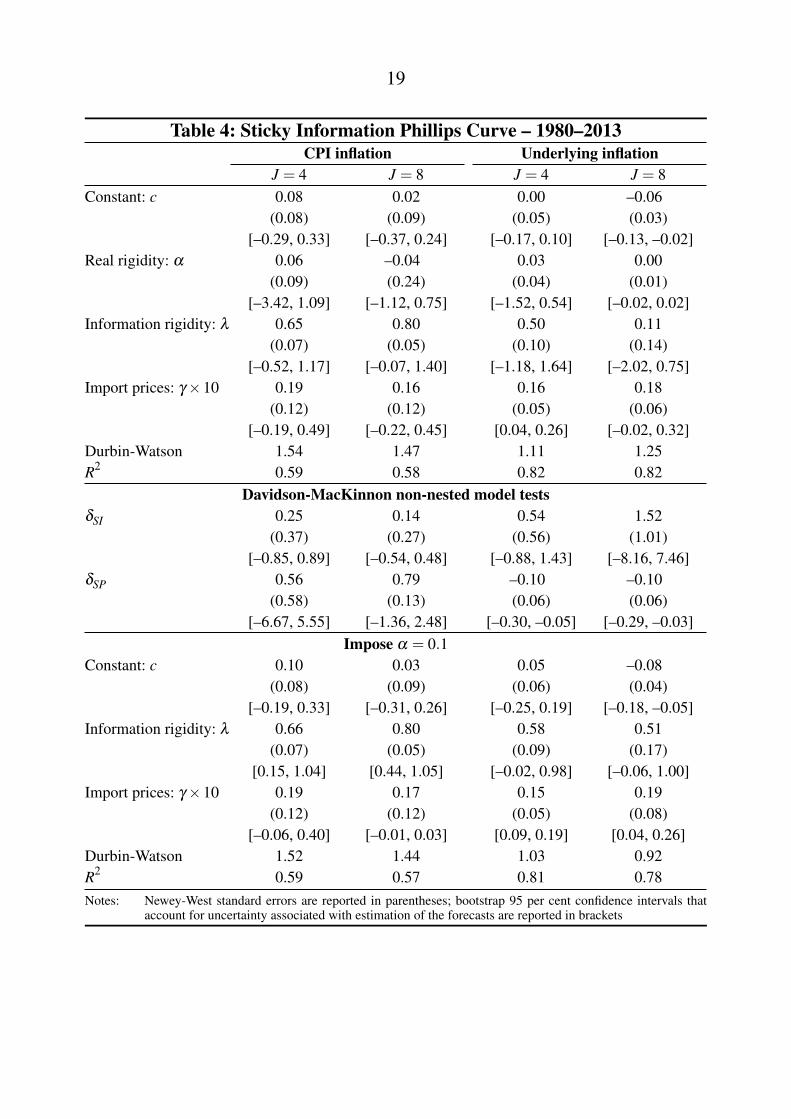
Table 4 reports estimates of the SIPC using data for the period 1980–2013,over which only the econometric forecasts are available; estimates are presentedfor truncation of the SIPC at both a one- and two-year horizon.9 In each case,the estimated degree of information rigidity is theoretically consistent. For CPIinflation, the estimated values for λ indicate that firms on average update theirinformation set each 3–5 quarters. The estimated degree of information rigidity islarger over the 1980–2013 sample than the 1995–2013 sample largely because CPIinflation behaved inertially during the 1980s and the period of disinflation, whichis consistent with the SIPC model. But despite the inertial behaviour of underlyinginflation over the 1980–2013 period, the estimated degree of information rigidityis relatively low. This is because the long-horizon underlying inflation forecastssubstantially overpredicted inflation during the disinflation (see Figure 2). A highdegree of information rigidity would place substantial weight on these poorlyperforming long-horizon forecasts, reducing the empirical fit of the SIPC.

Because of the weak contemporaneous correlation between inflation and theoutput gap, the estimated degree of real rigidity is large (α is small) for allSIPC specifications reported in Table 4. Imposing the degree of real rigidity tobe α = 0.1 has little effect on the estimated degree of information rigidity or thefit of the SIPC, except for the underlying inflation SIPC truncated at a two-yearhorizon. As explained earlier, when the freely estimated degree of informationrigidity is large, the coefficient on the output gap is insensitive to the parameterα . The share of the variation in inflation explained by the SIPC is high, largelybecause the model captures the mean shift in the early 1990s.

9 See Appendix B for estimates over the shorter 1980–1990 sample period.

19

Table 4: Sticky Information Phillips Curve – 1980–2013CPI inflation Underlying inflation

J = 4 J = 8 J = 4 J = 8Constant: c 0.08 0.02 0.00 –0.06

(0.08) (0.09) (0.05) (0.03)[–0.29, 0.33] [–0.37, 0.24] [–0.17, 0.10] [–0.13, –0.02]

Real rigidity: α 0.06 –0.04 0.03 0.00(0.09) (0.24) (0.04) (0.01)

[–3.42, 1.09] [–1.12, 0.75] [–1.52, 0.54] [–0.02, 0.02]Information rigidity: λ 0.65 0.80 0.50 0.11

(0.07) (0.05) (0.10) (0.14)[–0.52, 1.17] [–0.07, 1.40] [–1.18, 1.64] [–2.02, 0.75]

Import prices: γ ×10 0.19 0.16 0.16 0.18(0.12) (0.12) (0.05) (0.06)

[–0.19, 0.49] [–0.22, 0.45] [0.04, 0.26] [–0.02, 0.32]Durbin-Watson 1.54 1.47 1.11 1.25R2 0.59 0.58 0.82 0.82

Davidson-MacKinnon non-nested model testsδSI 0.25 0.14 0.54 1.52

(0.37) (0.27) (0.56) (1.01)[–0.85, 0.89] [–0.54, 0.48] [–0.88, 1.43] [–8.16, 7.46]

δSP 0.56 0.79 –0.10 –0.10(0.58) (0.13) (0.06) (0.06)

[–6.67, 5.55] [–1.36, 2.48] [–0.30, –0.05] [–0.29, –0.03]Impose α = 0.1

Constant: c 0.10 0.03 0.05 –0.08(0.08) (0.09) (0.06) (0.04)

[–0.19, 0.33] [–0.31, 0.26] [–0.25, 0.19] [–0.18, –0.05]Information rigidity: λ 0.66 0.80 0.58 0.51

(0.07) (0.05) (0.09) (0.17)[0.15, 1.04] [0.44, 1.05] [–0.02, 0.98] [–0.06, 1.00]

Import prices: γ ×10 0.19 0.17 0.15 0.19(0.12) (0.12) (0.05) (0.08)

[–0.06, 0.40] [–0.01, 0.03] [0.09, 0.19] [0.04, 0.26]Durbin-Watson 1.52 1.44 1.03 0.92R2 0.59 0.57 0.81 0.78Notes: Newey-West standard errors are reported in parentheses; bootstrap 95 per cent confidence intervals that

account for uncertainty associated with estimation of the forecasts are reported in brackets

20

4.3 Comparing the SIPC and the NKPC

For the 1980–2013 period as a whole, the SIPC appears to provide a plausiblemodel of inflation. But is the sticky-information model a better descriptionof inflation dynamics than the sticky-price model? Because the SIPC andNKPC models are non-nested, discriminating between the two models is not asstraightforward as imposing restrictions on the estimated parameters of the SIPC.The first set of tests used to discriminate between the two price-setting modelsare Davidson and MacKinnon (2002) non-nested model tests. Under the nullhypothesis that the sticky-information model is correct, the SIPC is augmentedwith NKPC fitted values and re-estimated:

πt = c +[

1−λ

λ

]αxt +(1−λ )

∑Jj=0 λ

jEt− j−1 [πt +α∆xt ]+ γπmt

+δSPπNKPCt + εt ,

(9)

where πNKPCt is the fitted values from estimation of the NKPC, Equation (7).

Under the null hypothesis that the SIPC is correct, the NKPC fitted values have noadditional explanatory power for inflation, and the coefficient δSP is insignificantlydifferent from zero. Rejection of the hypothesis δSP = 0 provides evidence infavour of the NKPC. Similarly, under the null hypothesis that the sticky-pricemodel is correct, the NKPC model is augmented with SIPC fitted values and re-estimated:

πt = c+ρxt +βEt[πt+1

]+ γπ

mt +δSIπ

SIPCt + εt , (10)

where πSIPCt is the fitted values from estimation of the SIPC, Equation (4).

Rejection of the hypothesis δSI = 0 provides evidence in favour of the SIPC model.

The middle panel of Table 4 reports estimates for these non-nested model tests. Foreach inflation measure and truncation length, we cannot reject the null hypothesisδSP = 0 in testing the null hypothesis that the SIPC is the correct model, orthe hypothesis that δSI = 0 in testing the null hypothesis that the NKPC is thecorrect model. This is true even with ordinary standard errors, that do not allowfor the fact that the forecasts are generated regressors. Thus, the Davidson andMacKinnon (2002) non-nested model tests provide inconclusive evidence.

Estimation of an encompassing model provides an alternative means to test theSIPC against the NKPC. This involves jointly estimating the parameters for each

21

model:

πt = c+ωπSIPCt (α,λ )+(1−ω)π

NKPCt (ρ,β )+ γπ

mt + εt , (11)

where ω is the weight on the SIPC model, πSIPCt (α,λ ) is SIPC inflation, given

by the right-hand-side of Equation (4) excluding the import price term, andπ

NKPCt (ρ,β ) is NKPC inflation, given by the right-hand-side of Equation (7),

excluding the import price term. Because the encompassing regression is highlynon-linear in five parameters, the SIPC parameters are restricted to be theoreticallyconsistent, α > 0 and 0 < λ < 1, and the sum of the weights on the models isconstrained to unity, 0 < ω < 1.

The first two columns of Table 5 report encompassing test results, for CPI andunderlying inflation. The results suggest that the forward-looking NKPC is abetter description of inflation dynamics over the 1980–2013 period than the SIPCmodel: the coefficient ω , the weight on the SIPC model relative to the NKPCmodel, is small. Because the estimated weight on the SIPC is small, the SIPCparameters α and λ are imprecisely estimated: as ω approaches zero, a wide rangeof coefficients for the SIPC fits the data almost equally well. Because the outputgap enters both the SIPC and the NKPC when ω is above zero, the encompassingtest cannot precisely pin down the output gap parameters α and ρ in each model:identification comes only via the non-linearity in the SIPC. This imprecision isevident for the underlying inflation encompassing model.

The NKPC model appears to fit the data better in part because, as shown inFigure 2, the long-horizon real-time forecasts substantially overpredicted inflationrelative to the short-horizon forecasts during the early 1990s disinflation. Thereal-time forecast error was smaller for short-horizon forecasts because they placemore weight on recent inflation outcomes and less weight on the estimated long-run mean inflation rate, which was slow to update during the disinflationary period.Thus, the SIPC model, which places weight on dated long-horizon forecasts,substantially overpredicts inflation during the disinflation, except with very lowlevels of information rigidity. This is particularly apparent with the calibration ofthe SIPC proposed by Mankiw and Reis (2002), as shown in Figure 4.

22

Table 5: Encompassing Model Test – 1980–2013Encompassing test NKPC Hybrid NKPCCPI Underlying CPI Underlying CPI Underlying

inflation inflation inflation inflation inflation inflationJ = 8 J = 8

Constant 0.08 0.05 0.09 0.07 0.09 0.06(0.07) (0.04) (0.07) (0.04) (0.07) (0.04)

[–0.15, 0.23] [–0.04, 0.13] [–0.15, 0.24] [–0.08, 0.20] [–0.12, 0.23] [–0.07, 0.15]α 2.68 0.75

(204.6) (2.98)[−∞,∞] [–25.28,

23.03]λ 0.95 0.18

(22.64) (1.14)[–142.64,112.51]

[–1.26, 1.53]

ρ 0.02 –0.62 0.02 0.00 0.02 0.00(1.01) (2.72) (0.03) (0.02) (0.03) (0.02)

[–2.04, 1.66] [–2.14, 0.35] [–0.11, 0.11] [–0.07, 0.06] [–0.10, 0.11] [–0.08, 0.06]β 0.85 0.89 0.84 0.90 0.80 0.82

(2.71) (0.05) (0.06) (0.05) (0.16) (0.20)[–6.01, 6.39] [0.76, 0.98] [0.61, 1.03] [0.68, 1.03] [0.11, 1.32] [–0.61, 1.62]

γ ×10 0.12 0.11 0.12 0.10 0.12 0.09(0.11) (0.04) (0.11) (0.04) (0.12) (0.04)

[–0.15, 0.36] [0.01, 0.18] [–0.14, 0.33] [0.02, 0.16] [–0.25, 0.35] [0.03, 0.16]ω 0.01 0.15

(3.09) (0.42)[–0.16, 0.11] [–0.17, 0.41]

LDV 0.05 0.08(0.16) (0.18)

[–0.72, 0.51] [–0.39, 0.47]DW 1.91 1.91 1.91 2.06 1.98 2.17R2 0.60 0.84 0.60 0.84 0.60 0.84Notes: Newey-West standard errors are reported in parentheses; bootstrap 95 per cent confidence intervals that

account for uncertainty associated with estimation of the forecasts are reported in brackets; LDV denoteslagged dependent variable; DW denotes Durbin-Watson

23

Separately estimated NKPC equations reinforce the evidence in favour of thesticky-price model. The estimated coefficient on forward-looking NKPC inflationis similar in the encompassing model and the NKPC model, and the fit of theNKPC model for CPI and underlying inflation is no worse than the encompassingmodel (see Table 5). The hybrid NKPC model augments the NKPC with a laggeddependent variable, providing a reduced-form means of capturing the inflationinertia that the SIPC builds in from microfoundations. The estimated weight onlagged inflation is small, consistent with the small estimated weight on the SIPCin the encompassing model.

Figure 4: Predicted Quarterly Underlying Inflation

0.0

0.5

1.0

1.5

2.0

2.5

3.0

0.0

0.5

1.0

1.5

2.0

2.5

3.0

SIPC: J = 8

2013

%%

Underlying inflation

NKPC

20072001199519891983

Note: SIPC and NKPC have been calibrated using Mankiw and Reis (2002) parameter values:α = 0.1 and λ = 0.75

4.4 Adaptive Expectations Phillips Curve

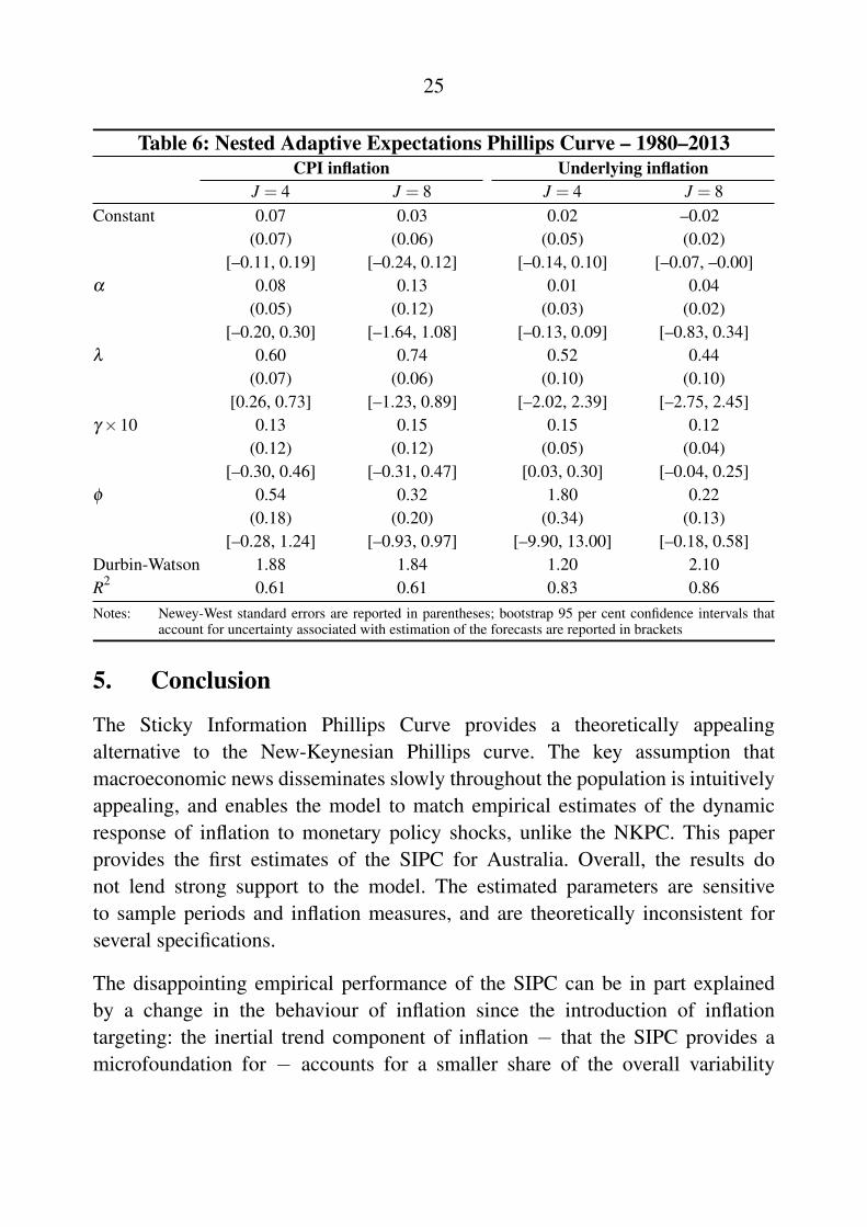
The previous section sought to distinguish between the non-nested SIPC andNKPC models, the two most prominent Phillips curve models in the literature. Anested alternative to the SIPC is the adaptive expectations Phillips curve (AEPC).The SIPC model reduces to a distributed-lag AEPC under the assumption thatexpected inflation is equal to current inflation, and expected changes in the output

24

gap are equal to zero. Accordingly, the SIPC can be expressed as an AEPC plusexpectational deviations between the two models:

πt = c +[

1−λ

λ

]αxt +(1−λ )

∑Jj=0 λ

jπt− j

+φ (1−λ )∑J

j=0 λjEt− j−1

[(πt −πt− j

)+α∆xt

]+ γπ

mt + εt .

(12)

Table 6 reports parameter estimates for Equation (12). Under the null hypothesisthat the SIPC is correct φ = 1, and under the null hypothesis that the AEPCis correct φ = 0. Empirically distinguishing between the two models requiresthe SIPC rational expectations forecasts to substantially outperform the AEPCrandom walk forecasts; if the rational expectations forecasts are identical to therandom walk forecasts, the SIPC model is indistinguishable from a distributed-lag AEPC. Particularly over the low-inflation period, the random walk benchmarkhas been shown to be difficult to improve upon: Atkeson and Ohanian (2001)find that Phillips curve-based forecasts do not outperform random walk forecastsfor US inflation after 1984, and Heath et al (2004) report similar evidence forAustralia. This means that tests seeking to distinguish between the SIPC andAEPC models have low power. Reflecting this, the bootstrap confidence intervalsfor the parameter φ in Equation (12) are wide enough to be consistent with boththe SIPC and AEPC models.

Although the SIPC and AEPC equations have similar fit, they have differenttheoretical implications for the behaviour of inflation. Mankiw and Reis (2002)show that, in response to a demand shock, inflation and output overshoot in theAEPC model, but behave inertially and do not overshoot in the SIPC model.Tests based on the dynamic response to shocks may be more informative fordistinguishing between the SIPC and AEPC models than fit comparisons. Thisis left for further work.

25

Table 6: Nested Adaptive Expectations Phillips Curve – 1980–2013CPI inflation Underlying inflation

J = 4 J = 8 J = 4 J = 8Constant 0.07 0.03 0.02 –0.02

(0.07) (0.06) (0.05) (0.02)[–0.11, 0.19] [–0.24, 0.12] [–0.14, 0.10] [–0.07, –0.00]

α 0.08 0.13 0.01 0.04(0.05) (0.12) (0.03) (0.02)

[–0.20, 0.30] [–1.64, 1.08] [–0.13, 0.09] [–0.83, 0.34]λ 0.60 0.74 0.52 0.44

(0.07) (0.06) (0.10) (0.10)[0.26, 0.73] [–1.23, 0.89] [–2.02, 2.39] [–2.75, 2.45]

γ ×10 0.13 0.15 0.15 0.12(0.12) (0.12) (0.05) (0.04)

[–0.30, 0.46] [–0.31, 0.47] [0.03, 0.30] [–0.04, 0.25]φ 0.54 0.32 1.80 0.22

(0.18) (0.20) (0.34) (0.13)[–0.28, 1.24] [–0.93, 0.97] [–9.90, 13.00] [–0.18, 0.58]

Durbin-Watson 1.88 1.84 1.20 2.10R2 0.61 0.61 0.83 0.86Notes: Newey-West standard errors are reported in parentheses; bootstrap 95 per cent confidence intervals that

account for uncertainty associated with estimation of the forecasts are reported in brackets

5. Conclusion

The Sticky Information Phillips Curve provides a theoretically appealingalternative to the New-Keynesian Phillips curve. The key assumption thatmacroeconomic news disseminates slowly throughout the population is intuitivelyappealing, and enables the model to match empirical estimates of the dynamicresponse of inflation to monetary policy shocks, unlike the NKPC. This paperprovides the first estimates of the SIPC for Australia. Overall, the results donot lend strong support to the model. The estimated parameters are sensitiveto sample periods and inflation measures, and are theoretically inconsistent forseveral specifications.

The disappointing empirical performance of the SIPC can be in part explainedby a change in the behaviour of inflation since the introduction of inflationtargeting: the inertial trend component of inflation − that the SIPC provides amicrofoundation for − accounts for a smaller share of the overall variability

26

in inflation than in the past. Accordingly, including data prior to the inflation-targeting period in the estimation sample improves the performance of the SIPC.However, the NKPC appears to fit the data at least as well as the SIPC. Theperformance of the SIPC is particularly affected by the weak connection betweenthe real and nominal side of the model. Furthermore, the NKPC is better ableto explain the disinflation because it places less weight on long-horizon inflationforecasts, which (based on model estimates) substantially overpredicted inflationin the early 1990s. Taking account of differences in forecast measures used andrestrictions placed on the model parameters, these findings are broadly in linewith evidence for the United States and Europe.

While the results provide little support for the SIPC, particularly over the low-inflation period, they should not necessarily be taken as evidence against theimportance of information rigidities. Since the introduction of inflation targeting,it has become more difficult to model inflation. The share of variation in inflationexplained by a wide range of models has fallen together with the overall variationin inflation. Few models can now outperform a forecast of constant inflation of2.5 per cent (midpoint of the RBA’s target band). The poor performance of theSIPC over the low-inflation period in part reflects this more general finding, andnot necessarily a rejection of the importance of information rigidities. Alternatetests find evidence consistent with information rigidities. For example, Coibionand Gorodnichenko (2012) show that the response of survey forecast errorsto economic shocks supports the sticky-information model. The behaviour ofconsumer inflation expectations is also consistent with slow diffusion of economicnews throughout the population (Carroll 2003). The core assumption of theSIPC that macroeconomic news disseminates slowly throughout the populationis attractive, and the SIPC provides a useful framework for thinking through theeffects on inflation. One possible means of improving the performance of the SIPCmight be to introduce state-dependence in the frequency with which firms updatetheir expectations. This would allow inflation to respond quickly to some shocks,but retain the predicted inertial response to monetary policy shocks.

27

Appendix A: Confidence Intervals for Econometric Forecasts

Ordinary standard errors generated by estimation of the SIPC with the econometricforecasts do not take forecast uncertainty into account. This is the generatedregressors problem discussed by Pagan (1986). To allow for uncertainty causedby estimation of the forecasts, the bootstrap procedure outlined by Kahn andZhu (2006) is followed. The first step in the procedure requires generatingalternate histories of the data. The vector autoregression model

Yt = β (L)Yt + εt (A1)

is estimated using each of the forecast and explanatory variables listed in Table 1,for the period 1964–2013. The lag length is set at 8 quarters, guided by the AICcriteria. The first alternate history of data is created by repeated resampling (withreplacement) from the vector of estimated residuals εt , using the first L-quartersof data for the lagged dependent variables. Data for an initial burn-in-period of100 quarters is discarded, leaving a simulated set of data for the period 1964–2013.This procedure is repeated N = 500 times to produce a set of alternate histories ofdata.

For each history of data, the forecast procedure outlined in Section 3.1 is usedto estimate econometric forecasts for CPI inflation, underlying inflation and thechange in the output gap. Use of each alternate set of forecasts to estimate theSIPC produces a distribution of parameter estimates and standard errors for eachregression coefficient. For each set of data i and regression parameter βk the teststatistic

t∗i,k =βk,i − βk

σk,i(A2)

is calculated, where βk,i is the estimated regression coefficient for parameter kusing alternate history of data i, σk,i is its estimated standard error, and βk is theparameter estimate using the observed data. Taking the 2.5 and 97.5 percentilesof t∗i,k produces bootstrapped 95 per cent critical values t∗L,k and t∗U,k for regressionparameter k. Using these critical values, a percentile-t interval can be calculatedfor regression parameter k: [

βk − t∗U,kσk, βk − t∗L,kσk

]. (A3)

28

Note that the percentile-t confidence interval is not guaranteed to contain theparameter estimate βk. For example, suppose each bootstrapped estimate βk,i > βk,then t∗L,k > 0 and the upper bound of the confidence interval is less than theparameter estimate βk.

29

Appendix B: SIPC Estimates for 1980–1990

Table B1: Sticky Information Phillips Curve – 1980–1990CPI inflation Underlying inflation

J = 4 J = 8 J = 4 J = 8Constant: c 1.55 0.94 –0.10 –0.09

(0.43) (0.50) (0.06) (0.05)[–11.70, 12.68] [–8.54, 9.41] [–0.32, 0.07] [–0.41, 0.09]

Real rigidity: α –1.21 –1.14 0.00 0.00(1.01) (0.84) (0.01) (0.01)

[–5.60, 1.56] [–4.79, 1.17] [–0.03, 0.02] [–0.05, 0.03]Information rigidity: λ 0.92 0.91 0.11 0.12

(0.06) (0.05) (0.19) (0.19)[–0.06, 1.70] [–0.58, 1.61] [–2.68, 1.62] [–3.50, 1.45]

Import prices: γ ×10 0.55 0.48 0.25 0.25(0.08) (0.11) (0.09) (0.09)

[–0.42, 1.19] [–0.08, 0.13] [–1.03, 0.74] [–1.01, 0.72]Durbin-Watson 1.56 1.54 1.48 1.50R2 0.32 0.31 0.37 0.38Notes: Newey-West standard errors are reported in parentheses; bootstrap 95 per cent confidence intervals that

account for uncertainty associated with estimation of the forecasts are reported in brackets

30

References

Atkeson A and LE Ohanian (2001), ‘Are Phillips Curves Useful for ForecastingInflation?’, Federal Reserve Bank of Minneapolis Quarterly Review, 25(1),pp 2–11.

Ball L (1994), ‘Credible Disinflation with Staggered Price-Setting’, The AmericanEconomic Review, 84(1), pp 282–289.

Blanchard OJ and N Kiyotaki (1987), ‘Monopolistic Competition andthe Effects of Aggregate Demand’, The American Economic Review, 77(4),pp 647–666.

Carroll CD (2003), ‘Macroeconomic Expectations of Households andProfessional Forecasters’, The Quarterly Journal of Economics, 118(1),pp 269–298.

Christiano LJ, M Eichenbaum and CL Evans (1999), ‘Monetary PolicyShocks: What Have We Learned and to What End?’, in JB Taylor and M Woodford(eds), Handbook of Macroeconomics: Volume 1A, Handbooks in Economics, 15,Elsevier Science B.V., Amsterdam, pp 65–148.

Coibion O (2010), ‘Testing the Sticky Information Phillips Curve’, Review ofEconomics and Statistics, 92(1), pp 87–101.

Coibion O and Y Gorodnichenko (2012), ‘What Can Survey Forecasts Tell Usabout Information Rigidities?’, Journal of Political Economy, 120(1), pp 116–159.

Davidson R and JG MacKinnon (2002), ‘Bootstrap J Tests of Nonnested LinearRegression Models’, Journal of Econometrics, 109(1), pp 167–193.

Dopke J, J Dovern, U Fritsche and J Slacalek (2008), ‘Sticky InformationPhillips Curves: European Evidence’, Journal of Money, Credit and Banking,40(7), pp 1513–1519.

Fuhrer J and G Moore (1995), ‘Inflation Persistence’, The Quarterly Journal ofEconomics, 110(1), pp 127–159.

Galı J and M Gertler (1999), ‘Inflation Dynamics: A Structural EconometricAnalysis’, Journal of Monetary Economics, 44(2), pp 195–222.

31

Galı J, M Gertler and JD Lopez-Salido (2005), ‘Robustness of the Estimatesof the Hybrid New Keynesian Phillips Curve’, Journal of Monetary Economics,52(6), pp 1107–1118.

Heath A, I Roberts and T Bulman (2004), ‘Inflation in Australia: Measurementand Modelling’, in C Kent and S Guttmann (eds), The Future of InflationTargeting, Proceedings of a Conference, Reserve Bank of Australia, Sydney,pp 167–207.

Khan H and Z Zhu (2006), ‘Estimates of the Sticky-Information Phillips Curvefor the United States’, Journal of Money, Credit and Banking, 38(1), pp 195–207.

Kiley MT (2007), ‘A Quantitative Comparison of Sticky-Price and Sticky-Information Models of Price-Setting’, Journal of Money, Credit and Banking,39(Supplement 1), pp 101–125.

Korenok O (2008), ‘Empirical Comparison of Sticky Price and StickyInformation Models’, Journal of Macroeconomics, 30(3), pp 906–927.

Lucas Jr RE (1973), ‘Some International Evidence on Output-InflationTradeoffs’, The American Economic Review, 63(3), pp 326–334.

Mankiw NG (2001), ‘The Inexorable and Mysterious Tradeoff Between Inflationand Unemployment’, The Economic Journal, 111(471), pp C45–C61.

Mankiw NG and R Reis (2002), ‘Sticky Information Versus Sticky Prices: AProposal To Replace the New Keynesian Phillips Curve’, The Quarterly Journalof Economics, 117(4), pp 1295–1328.

Mavroeidis S, M Plagborg-Møller and JH Stock (2014), ‘Empirical Evidenceon Inflation Expectations in the New Keynesian Phillips Curve’, Journal ofEconomic Literature, 52(1), pp 124–188.

Norman D and A Richards (2010), ‘Modelling Inflation in Australia’, RBAResearch Discussion Paper No 2010-03.

Pagan A (1986), ‘Two Stage and Related Estimators and Their Applications’, TheReview of Economic Studies, 53(4), pp 517–538.

32

Reis R (2006), ‘Inattentive Producers’, The Review of Economic Studies, 73(3),pp 793–821.

Smets F and R Wouters (2007), ‘Shocks and Frictions in US Business Cycles: ABayesian DSGE Approach’, The American Economic Review, 97(3), pp 586–606.

Stock JH and MW Watson (1999), ‘Forecasting Inflation’, Journal of MonetaryEconomics, 44(2), pp 293–335.

Stock JH and MW Watson (2003), ‘Forecasting Output and Inflation: The Roleof Asset Prices’, Journal of Economic Literature, 41(3), pp 788–829.

Stock JH and MW Watson (2004), ‘Combination Forecasts of Output Growth ina Seven-Country Data Set’, Journal of Forecasting, 23(6), pp 405–430.

Stock JH and MW Watson (2007), ‘Why has U.S. Inflation Become Harder toForecast?’, Journal of Money, Credit and Banking, 39(Supplement s1), pp 3–33.

Tulip P and S Wallace (2012), ‘Estimates of Uncertainty around the RBA’sForecasts’, RBA Research Discussion Paper No 2012-07.