1

Research Design - - Topic 22 Multivariate Analysis of Variance

© 2009 R. C. Gardner, Ph.D.

Purpose and General Rationale

An Example Using SPSS GLM Multivariate

Basic mathematics

Assumptions

Multivariate OutputFollow-up TestsUnivariate Output

Multivariate Test Statistics

2

The purpose of multivariate analysis of variance in any of its forms is to perform an analysis of variance when there is more than one dependent variable. A multivariate analysis of variance can be performed on a single factor completely randomized design (see Gardner & Tremblay, 2007), a completely randomized factorial design, a single factor repeatedmeasures design, a split plot factorial design, a randomized blocks factorial design, etc. It is basically the equivalent of the corresponding univariate analysis of variance, but it has more than one dependent variable for each subject. The objective is to determine whether the main effects (and interactions where appropriate) are significant considering the variables as a set.This section will consider the single factor completely randomized design.

Purpose and General Rationale

3

The general rationale is comparable to that for principal components analysis. That is, we can form a weighted aggregate that accounts for as much of the between groups variation relative to the within groups variation as possible. Then, once we have done this we can form another weighted aggregate to account for as much of the relative variation as possible, and we can continue this until we have accounted for all of the relative variation. For the single factor design, we will find that the number of weighted aggregates that can be formed is equal to the number of groups minus 1 (i.e., the degrees of freedom associated with the univariate effect), or the number of dependent variables, whichever is less.

4

Multivariate analysis of variance (MANOVA) has been used for two(seemingly contradictory) reasons.

(1.) To control Type I error.Since only one test of significance is made, the Type I error for the collection of tests is set at α. Thus by performing MANOVA on a series of dependent variables, the Type I error experimentwise is equal to α (but see Slide 12).

(2.) To maximize power.MANOVA maximally weights the various dependent measuresto obtain the greatest differentiation among the groups. Thus, assuming Ho false, MANOVA is most likely to detect thedifference.

An additional advantage is that MANOVA might identify an effect due to a pattern of means for specific variables that would not be detected if the variables were analyzed one at a time.

5

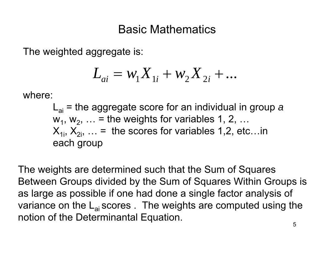
...2211 ++= iiai XwXwLThe weighted aggregate is:

where:Lai = the aggregate score for an individual in group aw1, w2, … = the weights for variables 1, 2, …X1i, X2i, … = the scores for variables 1,2, etc…in each group

The weights are determined such that the Sum of Squares Between Groups divided by the Sum of Squares Within Groups is as large as possible if one had done a single factor analysis ofvariance on the Lai scores . The weights are computed using the notion of the Determinantal Equation.

Basic Mathematics

6

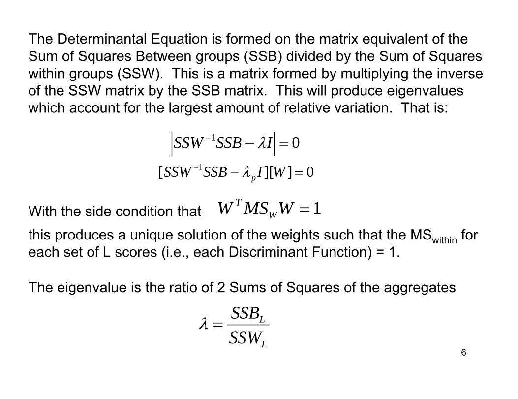
The Determinantal Equation is formed on the matrix equivalent of the Sum of Squares Between groups (SSB) divided by the Sum of Squares within groups (SSW). This is a matrix formed by multiplying the inverse of the SSW matrix by the SSB matrix. This will produce eigenvalueswhich account for the largest amount of relative variation. That is:

01 =−− ISSBSSW λ

0]][[ 1 =−− WISSBSSW pλ

1=WMSW WT

The eigenvalue is the ratio of 2 Sums of Squares of the aggregates

L

L

SSWSSB

=λ

this produces a unique solution of the weights such that the MSwithin for each set of L scores (i.e., each Discriminant Function) = 1.

With the side condition that

7

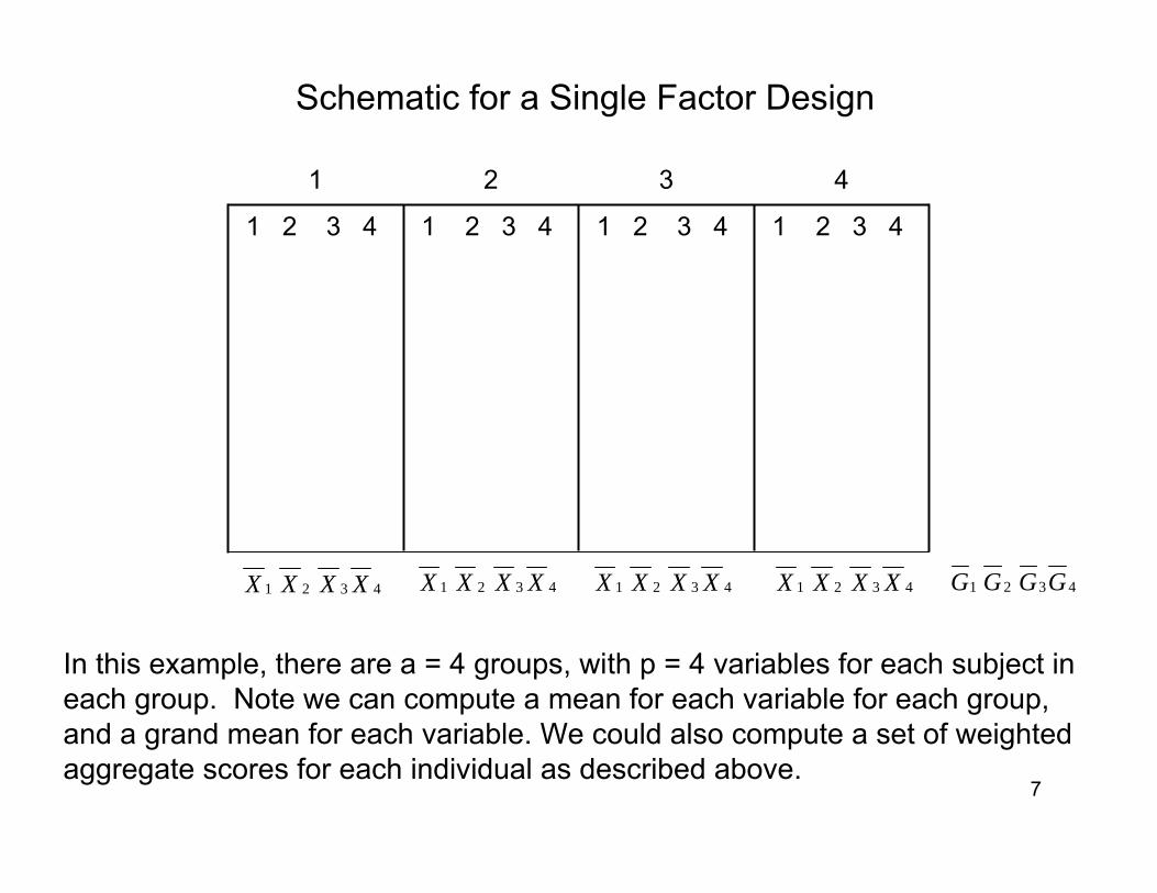
Schematic for a Single Factor Design

1 2 3 41 2 3 41 2 3 41 2 3 4

4321

4321 XXXX

In this example, there are a = 4 groups, with p = 4 variables for each subject in each group. Note we can compute a mean for each variable for each group, and a grand mean for each variable. We could also compute a set of weighted aggregate scores for each individual as described above.

4321 GGGG4321 XXXX 4321 XXXX 4321 XXXX

8

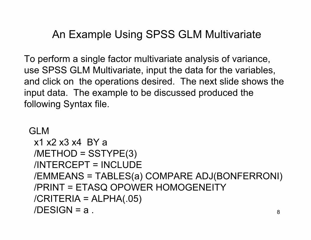
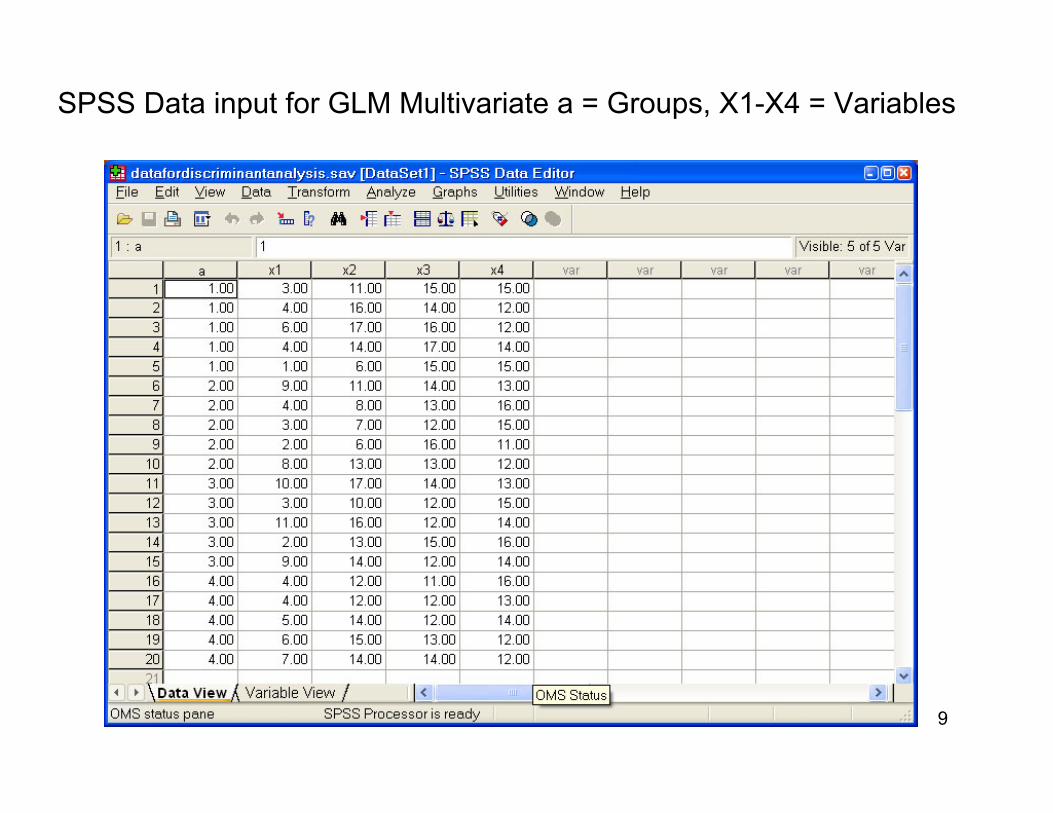
To perform a single factor multivariate analysis of variance, use SPSS GLM Multivariate, input the data for the variables, and click on the operations desired. The next slide shows the input data. The example to be discussed produced the following Syntax file.

GLMx1 x2 x3 x4 BY a/METHOD = SSTYPE(3)/INTERCEPT = INCLUDE/EMMEANS = TABLES(a) COMPARE ADJ(BONFERRONI)/PRINT = ETASQ OPOWER HOMOGENEITY/CRITERIA = ALPHA(.05)/DESIGN = a .

An Example Using SPSS GLM Multivariate

9

SPSS Data input for GLM Multivariate a = Groups, X1-X4 = Variables

10

Multivariate Testsd

.998 1902.588b 4.000 13.000 .000 .998 7610.353 1.000

.002 1902.588b 4.000 13.000 .000 .998 7610.353 1.000585.412 1902.588b 4.000 13.000 .000 .998 7610.353 1.000585.412 1902.588b 4.000 13.000 .000 .998 7610.353 1.000

1.396 3.266 12.000 45.000 .002 .465 39.187 .982.141 3.170 12.000 34.686 .004 .479 31.949 .932

2.911 2.830 12.000 35.000 .008 .492 33.962 .9491.472 5.522c 4.000 15.000 .006 .596 22.087 .913

Pillai's TraceWilks' LambdaHotelling's TraceRoy's Largest RootPillai's TraceWilks' LambdaHotelling's TraceRoy's Largest Root

EffectIntercept

a

Value F Hypothesis df Error df Sig.Partial EtaSquared

Noncent.Parameter

ObservedPowera

Computed using alpha = .05a.

Exact statisticb.

The statistic is an upper bound on F that yields a lower bound on the significance level.c.

Design: Intercept+ad.

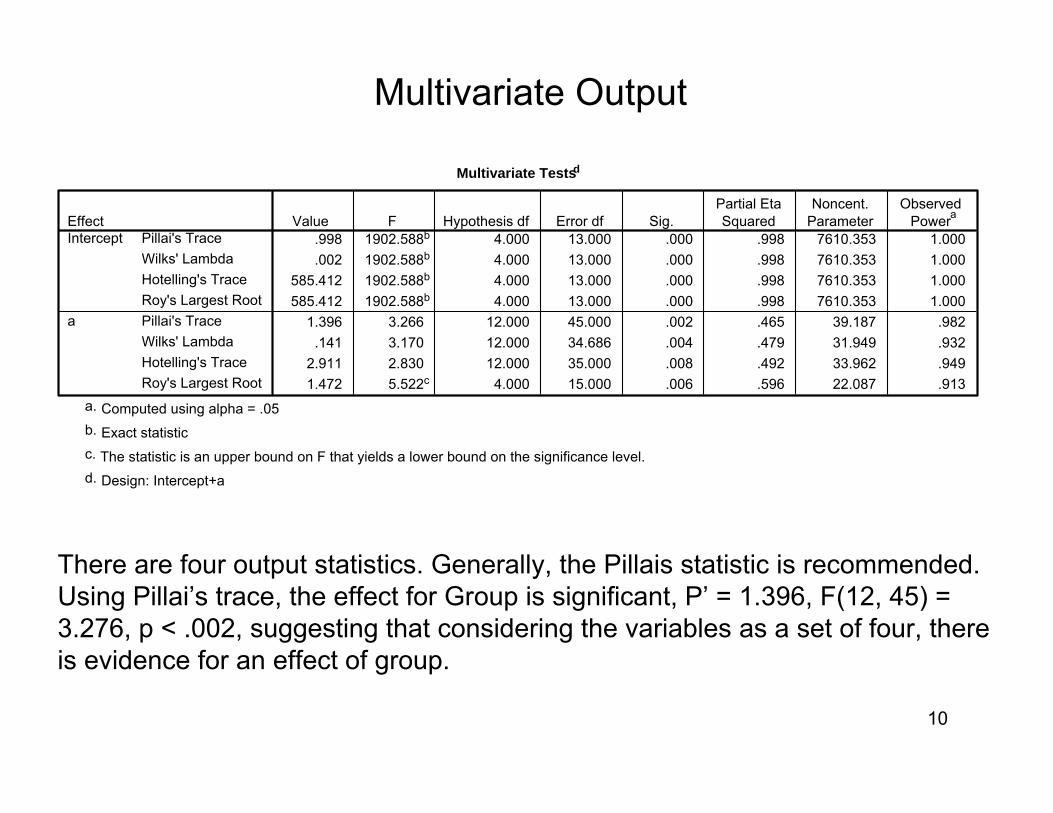
Multivariate Output

There are four output statistics. Generally, the Pillais statistic is recommended. Using Pillai’s trace, the effect for Group is significant, P’ = 1.396, F(12, 45) = 3.276, p < .002, suggesting that considering the variables as a set of four, there is evidence for an effect of group.

11

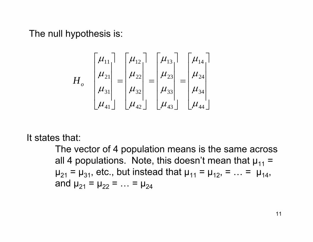
The null hypothesis is:

⎥⎥⎥⎥

⎦

⎤

⎢⎢⎢⎢

⎣

⎡

=

⎥⎥⎥⎥

⎦

⎤

⎢⎢⎢⎢

⎣

⎡

=

⎥⎥⎥⎥

⎦

⎤

⎢⎢⎢⎢

⎣

⎡

=

⎥⎥⎥⎥

⎦

⎤

⎢⎢⎢⎢

⎣

⎡

44

34

24

14

43

33

23

13

42

32

22

12

41

31

21

11

µµµµ

µµµµ

µµµµ

µµµµ

oH

It states that:The vector of 4 population means is the same across all 4 populations. Note, this doesn’t mean that µ11 = µ21 = µ31, etc., but instead that µ11 = µ12, = … = µ14, and µ21 = µ22 = … = µ24

12

1. Evaluate the univariate analyses of variance with α = .05. If so, do follow up tests of means as for a single dependent variable. This is the most common procedure that is used. For example, Kieffer,Reese & Thompson (2001), report that more than 70% of published articles use this approach even though it has been shown to depend on a misconception of Type I error (see, Huberty & Petoskey, 2001).

2. Evaluate the univariate analyses of variance with α = .05/p where p = the number of dependent variables. This approach is recommended by Tabachnick & Fidell (2001), though it seems then that the multivariate analysis is unnecessary (cf., Huberty & Morris, 1989). Marascuilo and Levin (1983) recommend post hoc contrasts with α = .05/p.

Follow-up Tests

13

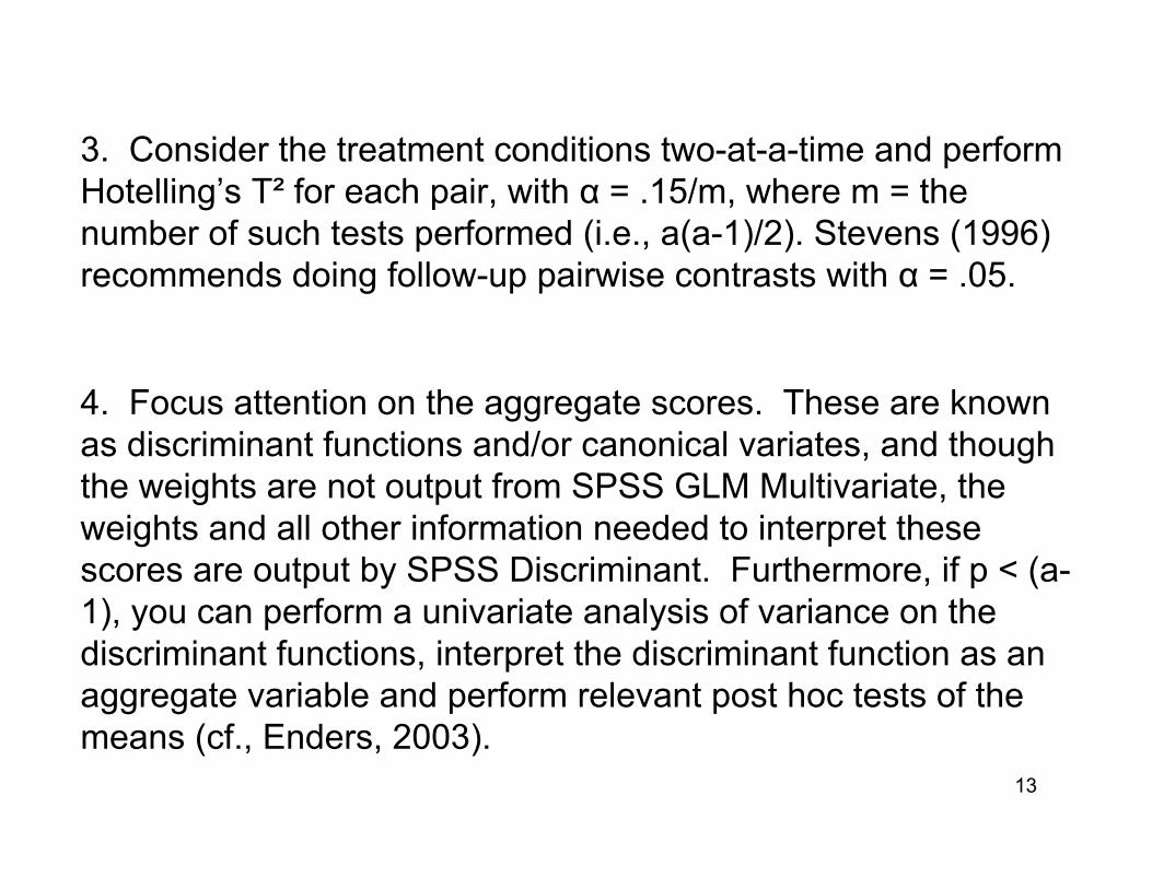
4. Focus attention on the aggregate scores. These are known as discriminant functions and/or canonical variates, and though the weights are not output from SPSS GLM Multivariate, the weights and all other information needed to interpret these scores are output by SPSS Discriminant. Furthermore, if p < (a-1), you can perform a univariate analysis of variance on the discriminant functions, interpret the discriminant function as an aggregate variable and perform relevant post hoc tests of the means (cf., Enders, 2003).

3. Consider the treatment conditions two-at-a-time and perform Hotelling’s T² for each pair, with α = .15/m, where m = the number of such tests performed (i.e., a(a-1)/2). Stevens (1996) recommends doing follow-up pairwise contrasts with α = .05.

14

Levene's Test of Equality of Error Variancesa

7.427 3 16 .0022.071 3 16 .144

.341 3 16 .7961.012 3 16 .413

x1x2x3x4

F df1 df2 Sig.

Tests the null hypothesis that the error variance of thedependent variable is equal across groups.

Design: Intercept+aa.

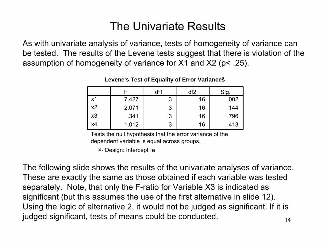
As with univariate analysis of variance, tests of homogeneity of variance can be tested. The results of the Levene tests suggest that there is violation of the assumption of homogeneity of variance for X1 and X2 (p< .25).

The Univariate Results

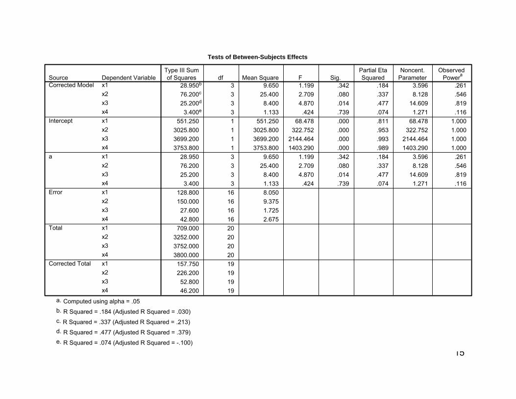
The following slide shows the results of the univariate analyses of variance. These are exactly the same as those obtained if each variable was tested separately. Note, that only the F-ratio for Variable X3 is indicated as significant (but this assumes the use of the first alternative in slide 12). Using the logic of alternative 2, it would not be judged as significant. If it is judged significant, tests of means could be conducted.

15

Tests of Between-Subjects Effects

28.950b 3 9.650 1.199 .342 .184 3.596 .26176.200c 3 25.400 2.709 .080 .337 8.128 .54625.200d 3 8.400 4.870 .014 .477 14.609 .819

3.400e 3 1.133 .424 .739 .074 1.271 .116551.250 1 551.250 68.478 .000 .811 68.478 1.000

3025.800 1 3025.800 322.752 .000 .953 322.752 1.0003699.200 1 3699.200 2144.464 .000 .993 2144.464 1.0003753.800 1 3753.800 1403.290 .000 .989 1403.290 1.000

28.950 3 9.650 1.199 .342 .184 3.596 .26176.200 3 25.400 2.709 .080 .337 8.128 .54625.200 3 8.400 4.870 .014 .477 14.609 .819

3.400 3 1.133 .424 .739 .074 1.271 .116128.800 16 8.050150.000 16 9.375

27.600 16 1.72542.800 16 2.675

709.000 203252.000 203752.000 203800.000 20

157.750 19226.200 19

52.800 1946.200 19

Dependent Variablex1x2x3x4x1x2x3x4x1x2x3x4x1x2x3x4x1x2x3x4x1x2x3x4

SourceCorrected Model

Intercept

a

Error

Total

Corrected Total

Type III Sumof Squares df Mean Square F Sig.

Partial EtaSquared

Noncent.Parameter

ObservedPowera

Computed using alpha = .05a.

R Squared = .184 (Adjusted R Squared = .030)b.

R Squared = .337 (Adjusted R Squared = .213)c.

R Squared = .477 (Adjusted R Squared = .379)d.

R Squared = .074 (Adjusted R Squared = -.100)e.

16

Estimates

3.600 1.269 .910 6.2905.200 1.269 2.510 7.8907.000 1.269 4.310 9.6905.200 1.269 2.510 7.890

12.800 1.369 9.897 15.7039.000 1.369 6.097 11.903

14.000 1.369 11.097 16.90313.400 1.369 10.497 16.30315.400 .587 14.155 16.64513.600 .587 12.355 14.84513.000 .587 11.755 14.24512.400 .587 11.155 13.64513.600 .731 12.049 15.15113.400 .731 11.849 14.95114.400 .731 12.849 15.95113.400 .731 11.849 14.951

a1.002.003.004.001.002.003.004.001.002.003.004.001.002.003.004.00

Dependent Variablex1

x2

x3

x4

Mean Std. Error Lower Bound Upper Bound95% Confidence Interval

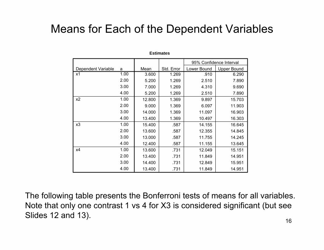
Means for Each of the Dependent Variables

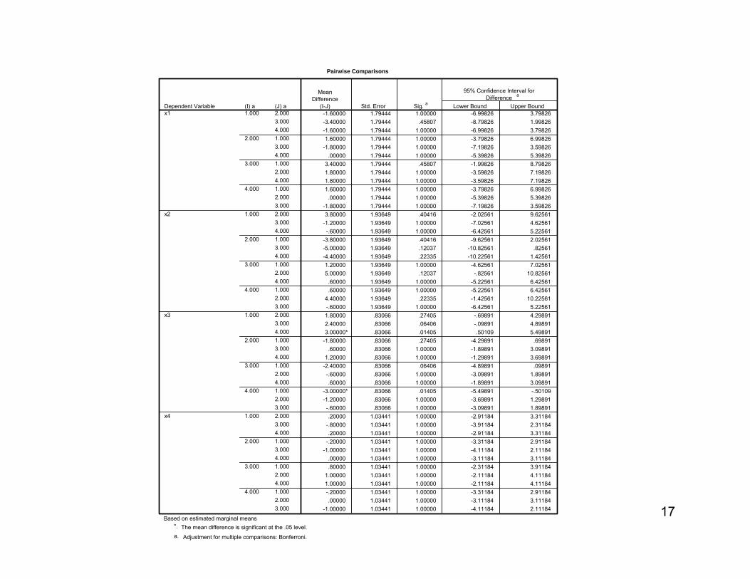
The following table presents the Bonferroni tests of means for all variables. Note that only one contrast 1 vs 4 for X3 is considered significant (but see Slides 12 and 13).

17

Pairwise Comparisons

-1.60000 1.79444 1.00000 -6.99826 3.79826-3.40000 1.79444 .45807 -8.79826 1.99826-1.60000 1.79444 1.00000 -6.99826 3.798261.60000 1.79444 1.00000 -3.79826 6.99826

-1.80000 1.79444 1.00000 -7.19826 3.59826.00000 1.79444 1.00000 -5.39826 5.39826

3.40000 1.79444 .45807 -1.99826 8.798261.80000 1.79444 1.00000 -3.59826 7.198261.80000 1.79444 1.00000 -3.59826 7.198261.60000 1.79444 1.00000 -3.79826 6.99826.00000 1.79444 1.00000 -5.39826 5.39826

-1.80000 1.79444 1.00000 -7.19826 3.598263.80000 1.93649 .40416 -2.02561 9.62561

-1.20000 1.93649 1.00000 -7.02561 4.62561-.60000 1.93649 1.00000 -6.42561 5.22561

-3.80000 1.93649 .40416 -9.62561 2.02561-5.00000 1.93649 .12037 -10.82561 .82561-4.40000 1.93649 .22335 -10.22561 1.425611.20000 1.93649 1.00000 -4.62561 7.025615.00000 1.93649 .12037 -.82561 10.82561.60000 1.93649 1.00000 -5.22561 6.42561.60000 1.93649 1.00000 -5.22561 6.42561

4.40000 1.93649 .22335 -1.42561 10.22561-.60000 1.93649 1.00000 -6.42561 5.225611.80000 .83066 .27405 -.69891 4.298912.40000 .83066 .06406 -.09891 4.898913.00000* .83066 .01405 .50109 5.49891

-1.80000 .83066 .27405 -4.29891 .69891.60000 .83066 1.00000 -1.89891 3.09891

1.20000 .83066 1.00000 -1.29891 3.69891-2.40000 .83066 .06406 -4.89891 .09891-.60000 .83066 1.00000 -3.09891 1.89891.60000 .83066 1.00000 -1.89891 3.09891

-3.00000* .83066 .01405 -5.49891 -.50109-1.20000 .83066 1.00000 -3.69891 1.29891-.60000 .83066 1.00000 -3.09891 1.89891.20000 1.03441 1.00000 -2.91184 3.31184

-.80000 1.03441 1.00000 -3.91184 2.31184.20000 1.03441 1.00000 -2.91184 3.31184

-.20000 1.03441 1.00000 -3.31184 2.91184-1.00000 1.03441 1.00000 -4.11184 2.11184

.00000 1.03441 1.00000 -3.11184 3.11184

.80000 1.03441 1.00000 -2.31184 3.911841.00000 1.03441 1.00000 -2.11184 4.111841.00000 1.03441 1.00000 -2.11184 4.11184-.20000 1.03441 1.00000 -3.31184 2.91184.00000 1.03441 1.00000 -3.11184 3.11184

-1.00000 1.03441 1.00000 -4.11184 2.11184

(J) a2.0003.0004.0001.0003.0004.0001.0002.0004.0001.0002.0003.0002.0003.0004.0001.0003.0004.0001.0002.0004.0001.0002.0003.0002.0003.0004.0001.0003.0004.0001.0002.0004.0001.0002.0003.0002.0003.0004.0001.0003.0004.0001.0002.0004.0001.0002.0003.000

(I) a1.000

2.000

3.000

4.000

1.000

2.000

3.000

4.000

1.000

2.000

3.000

4.000

1.000

2.000

3.000

4.000

Dependent Variablex1

x2

x3

x4

MeanDifference

(I-J) Std. Error Sig. a Lower Bound Upper Bound

95% Confidence Interval forDifference a

Based on estimated marginal meansThe mean difference is significant at the .05 level.*.

Adjustment for multiple comparisons: Bonferroni.a.

18

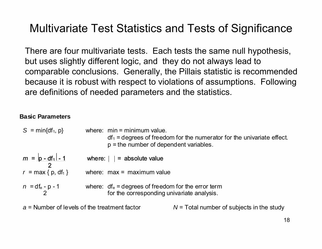
Basic Parameters

S = min{df1, p} where: min = minimum value. df1 = degrees of freedom for the numerator for the univariate effect.p = the number of dependent variables.

m = -p - df1 - - 1 where: * * = absolute value 2 r = max { p, df1 } where: max = maximum value n = dfe - p - 1 where: dfe = degrees of freedom for the error term 2 for the corresponding univariate analysis.

a = Number of levels of the treatment factor N = Total number of subjects in the study

m = -p - df1 - - 1 where: * * = absolute value 2

There are four multivariate tests. Each tests the same null hypothesis, but uses slightly different logic, and they do not always lead to comparable conclusions. Generally, the Pillais statistic is recommended because it is robust with respect to violations of assumptions. Following are definitions of needed parameters and the statistics.

Multivariate Test Statistics and Tests of Significance

19

Multivariate Tests of Significance

1. Pillais Trace

2. Hotelling-Lawley Trace

3. Wilks Lambda

4. Roy’s Largest Root

j

jPλ

λ+

∑=1

'

jH λ∑=

⎟⎟⎠

⎞⎜⎜⎝

⎛

+∏=Λ

jλ11

maxλ=R

20

)'(')(

PSrPSpaNF

−+−−

=1. Pillais Trace )()( 211 SdfSvdfpv e +==

2. Hotelling-Lawley Trace

)12()1(2

2 +++

=SmS

HSnF )1(2)12( 21 +=++= SnvSmSv

3. Wilks Lambda

b

b

vvF /1

1

/12 )1(

ΛΛ−

=

4. Roy’s Largest Root

1

2

vLvF =

Srdfvrv e +−== 21

F-ratios and degrees of freedom

2/)()1(' apNa +−−=

54

21

2

21

2

−+−

=dfp

dfpb

where

1)2/)((')( 1211 +−== dfpbavdfpv

21

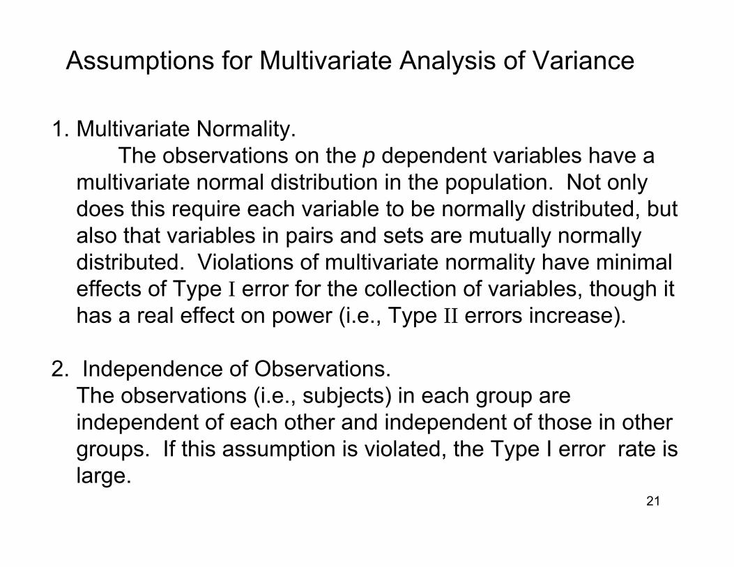
Assumptions for Multivariate Analysis of Variance

1. Multivariate Normality.The observations on the p dependent variables have a

multivariate normal distribution in the population. Not only does this require each variable to be normally distributed, but also that variables in pairs and sets are mutually normally distributed. Violations of multivariate normality have minimal effects of Type I error for the collection of variables, though it has a real effect on power (i.e., Type II errors increase).

2. Independence of Observations.The observations (i.e., subjects) in each group are independent of each other and independent of those in other groups. If this assumption is violated, the Type I error rate is large.

22

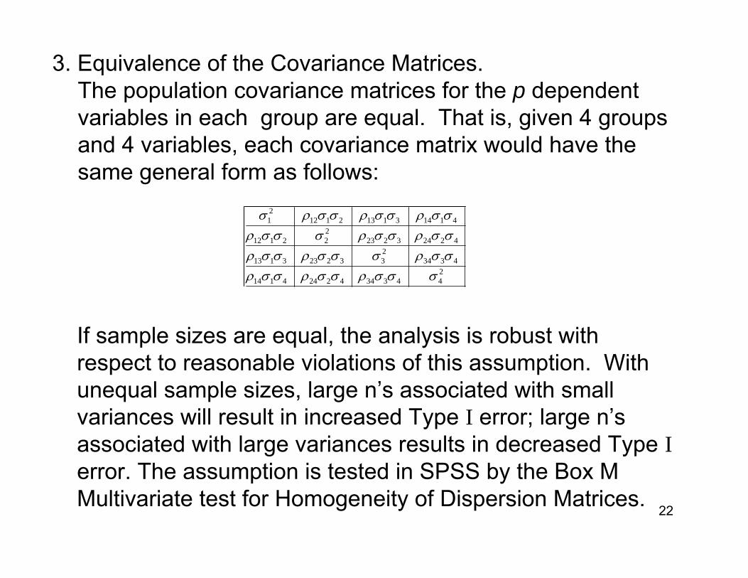
If sample sizes are equal, the analysis is robust with respect to reasonable violations of this assumption. With unequal sample sizes, large n’s associated with small variances will result in increased Type I error; large n’s associated with large variances results in decreased Type Ierror. The assumption is tested in SPSS by the Box M Multivariate test for Homogeneity of Dispersion Matrices.

3. Equivalence of the Covariance Matrices.The population covariance matrices for the p dependent variables in each group are equal. That is, given 4 groups and 4 variables, each covariance matrix would have the same general form as follows:

24433442244114

43342332233113

42243223222112

41143113211221

σσσρσσρσσρσσρσσσρσσρσσρσσρσσσρσσρσσρσσρσ

23

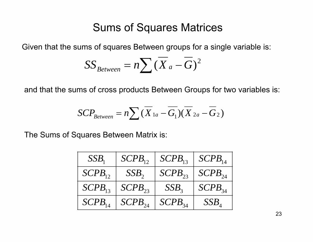
∑ −= 2)( GXnSS aBetween

∑ −−= ))(( 2211 GXGXnSCP aaBetween

Sums of Squares MatricesGiven that the sums of squares Between groups for a single variable is:

and that the sums of cross products Between Groups for two variables is:

The Sums of Squares Between Matrix is:

4342414

3432313

2423212

1413121

SSBSCPBSCPBSCPBSCPBSSBSCPBSCPBSCPBSCPBSSBSCPBSCPBSCPBSCPBSSB

24

∑∑ −= 2)( aaiWithin XXSS

∑∑ −−= ))(( 2211 aaiaaiWithin XXXXSCP

Given that the sums of squares Within groups for a single variable is:

and that the sums of cross products Within Groups for two variables is:

The Sums of Squares Within Matrix is:

4342414

3432313

2423212

1413121

SSWSCPWSCPWSCPWSCPWSSWSCPWSCPWSCPWSCPWSSWSCPWSCPWSCPWSCPWSSW

25

References

Enders, C.K. (2003). Performing multivariate group comparisons following statistically significant MANOVA. Measurement and Evaluation in Counseling and Development, 36, 40-56.

Gardner, R. C. & Tremblay, P.F. (2007). Essentials of Data Analysis: Statistics and Computer Applications. London, ON:UWO Bookstore

Huberty, C.J. & Morris, J.D. (1989). Multivariate analysis versus multiple univariate analyses. Psychological Bulletin, 105, 302-308.

Kieffer, K.M., Reese, R.J.& Thompson, B. (2001). Statistical techniquesemployed in AERJ and JCP articles from 1988 to 1997: A methodological review. Journal of Experimental Education, 69, 280-309.

Marascuilo, L.A. & Levin, J.R. (1983). Multivariate Statistics in the Social Sciences, Monterey, CA: Brooks/Cole.

Stevens, J. (1996). Applied Multivariate Statistics for the Social Sciences (Third Edition) Mahwah, NJ: Lawrence Erlbaum.