RESEARCH ARTICLE The bricycle: A bicycle in zero gravity ...

August 11, 2014 0:43 Vehicle System Dynamics brike˙paper20-revision

Vehicle System DynamicsVol. 00, No. 00, Month 200x, 1–15

RESEARCH ARTICLE

The bricycle:

A bicycle in zero gravity can be balanced or steered but not both

O. Dong, C. Graham, A. Grewal, C. Parrucci and A. Ruina∗

Cornell University, Ithaca, New York, USA

( Submitted August 11, 2014)

A bicycle or inverted pendulum can be balanced, that is kept nearly up-right, by accelerating the base. This balance is achieved by steering ona bicycle. Simultaneously one can also control the lateral position of thebase: changing of the track line of a bike or the position of hand un-der a balanced stick. We show here with theory and experiment that ifthe balance problem is removed, by making the system neutrally stablefor balance, one can’t simultaneously maintain balance and control theposition of the base.

We made a bricycle, essentially a bicycle with springy training wheels.The stiffness of the training wheel suspension can be varied from nearinfinite, making the bricycle into a tricycle, to zero, making it effec-tively a bicycle. The springy training wheels effectively reduce or evennegate gravity, at least for balance purposes. One might expect a smoothtransition from tricycle to bicycle as the stiffness is varied, in terms ofhandling, balance and feel. Not so. At an intermediate stiffness, whengravity is effectively zeroed, riders can balance easily but no longer turn.Small turns cause an intolerable leaning.

Thus there is a qualitative difference between bicycles and tricycles, adifference that cannot be met halfway.

Keywords: bricycle, bicycle, tricycle, controllability, balance, lean, steer, dynamics.

∗ Corresponding author: [email protected]

ISSN: 0042-3114 print/ISSN 1744-5159 onlinec© 200x Taylor & FrancisDOI: 10.1080/0042311YYxxxxxxxxhttp://www.informaworld.com


2

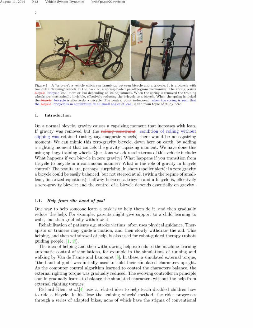
Figure 1. A ‘bricycle’: a vehicle which can transition between bicycle and a tricycle. It is a bicycle withtwo extra ‘training’ wheels at the back on a spring-loaded parallelogram mechanism. The spring resistsbicycle bricycle lean, more or less depending on its adjustment. When the spring is removed the trainingwheels are mechanically invisible, effectively reducing the bricycle to a bicycle. When the spring is lockedthe bicycle bricycle is effectively a tricycle. The neutral point in-between, when the spring is such thatthe bicycle bricycle is in equilibrium at all small angles of lean, is the main topic of study here.

1. Introduction

On a normal bicycle, gravity causes a capsizing moment that increases with lean.If gravity was removed but the rolling constraint condition of rolling withoutslipping was retained (using, say, magnetic wheels) there would be no capsizingmoment. We can mimic this zero-gravity bicycle, down here on earth, by addinga righting moment that cancels the gravity capsizing moment. We have done thisusing springy training wheels. Questions we address in terms of this vehicle include:What happens if you bicycle in zero gravity? What happens if you transition fromtricycle to bicycle in a continuous manner? What is the role of gravity in bicyclecontrol? The results are, perhaps, surprising. In short (spoiler alert): In zero gravitya bicycle could be easily balanced, but not steered at all (within the regime of small-lean, linearized equations); halfway between a tricycle and a bicycle is, effectivelya zero-gravity bicycle; and the control of a bicycle depends essentially on gravity.

1.1. Help from ‘the hand of god’

One way to help someone learn a task is to help them do it, and then graduallyreduce the help. For example, parents might give support to a child learning towalk, and then gradually withdraw it.

Rehabilitation of patients e.g. stroke victims, often uses physical guidance. Ther-apists or trainers may guide a motion, and then slowly withdraw the aid. Thishelping, and then withdrawal of help, is also used for robot-guided therapy (robotsguiding people, [1, 2]).

The idea of helping and then withdrawing help extends to the machine-learningautomatic control of simulations, for example in the simulations of running andwalking by Van de Panne and Lamouret [3]. In these, a simulated external torque,“the hand of god” was initially used to hold their simulated characters upright.As the computer control algorithm learned to control the characters balance, theexternal righting torque was gradually reduced. The evolving controller in principleshould gradually learns to balance the simulated characters without the help fromexternal righting torques.

Richard Klein et al.[4] uses a related idea to help teach disabled children howto ride a bicycle. In his ‘lose the training wheels’ method, the rider progressesthrough a series of adapted bikes, none of which have the stigma of conventional


3

p v

ba

n

pri gpr

m )

O

PQ

Figure 2. A Zero rest-length spring is the heart of the righting-moment mechanism. The spring isadjusted such that it’s force would be zero if the end of the connecting rod at P coincided with the pivot atQ; that would be the zero-length configuration. Because the spring compression is equal to the distance PQa zero rest-length tension spring between P and Q is simulated. The dimensions a and b can be adjustedby sliding the spring and base plate assembly up or down and re-clamping, changing the effective torsionalspring constant. See also the schematic in Fig. 3.

training wheels. The first has, instead of wheels, rolling pins (slightly bulged narrowcylinders) having a center of lateral curvature well above the riders center of mass.Such a bike stays securely upright. As the rider learns to pedal and steer, therollers are replaced with rollers with smaller rocking radius. Eventually regularbicycle wheels are used.

1.2. Signs of trouble

The gradually-weakening ‘hand of god’ approach to teaching might not always beeffective. Domingo et al.[5] had healthy subjects on a narrow or wide balance beam,mounted on a treadmill. For some of the subjects assistance was given by springs at-tached to a hip belt that applied restoring forces towards the beam center. On bothnarrow and wide beams, subjects learning without assistance had greater perfor-mance improvements in maintaining balance while walking, compared to subjectsin assisted groups (measured by failures per minute without assistance on the samebeam). Physical assistance seems to hinder learning in this context.

Indeed, the “guidance hypothesis” [6] is that the provision of too much external,augmented feedback during practice may cause the learner to develop a harmfuldependency on this source of feedback. The experience of errors and failures isimportant for learning. Physical guidance reduces the range of errors and hencehinders learning. Besides the experience of error, Domingo et al.[5] identify anotherfactor important to learning, the task-specific dynamics: “Having task dynamicsmore similar to the desired task would allow subjects to explore the state-space ofposition and velocity parameters and develop the ability to better control balance.”That is, despite its obvious appeal and common use, one can foresee problems withthe hand of god approach.

1.3. The Bricycle concept

Tricycles are easier to ride and steer compared to bicycles, at least for slow movingbeginners. Based on the intuitive appeal of ‘the hand of god’ approach, and ignoringthe forewarnings, we considered making a vehicle (a bricycle) which could, byadjustment, transition smoothly from a tricycle to bicycle. For example, a beginnercould start in tricycle-mode and change into bicycle-mode as she gains proficiency.


4

P

O

Q

ab

k

a sin

FS

ka sin

(c)

Q

a bP

O

Q

G

h

(b)(a)

Figure 3. a) Training wheel suspension. The rear wheels are connected to each other via a parallelogrammechanism. The connection between points P and Q is effectively a zero rest-length spring. The lengths aand b are adjustable. b) Force generated by the zero rest-length spring, is proportional to the length PQand the component of the force perpendicular to PQ is proportional to a sinφ. c) The restoring torquegenerated by the spring force Fs about point O is kba sinφ. This counters, less or more depending onparameters, the destabilizing gravitational torque mgh sinφ.

The initial idea was to avoid the discrete changes needed in the Klein sequence-of-thinner-and-thinner-wheels approach.

The bricycle concept is related to that of narrow tilting vehicles (or narrow trackvehicles, NTVs). NTVs are midway between a car and a motorcycle: they self-balance when stationary like a car and when moving they lean into turns like amotorcycle. Examples include the 1950s Ford Gyron, General Motors’ 1970s LeanMachine [7], and more recently, the Mercedes F-3000 Life-Jet and Nissan landglider. The controllers for NTVs tilt the vehicle using some combination of twostrategies: 1) Direct tilt control: an actuator on the longitudinal axis of the NTVproviding torque to tilt the vehicle [10]; 2) Steering tilt control: the steering angleapplied by the driver is modulated to control the tilt angle using countersteering[12–14]. The spring-righting on a bricycle is a special case of type (1) NTV control.Thus the problems with bicycle bricycle control that we describe below need tobe circumvented in NTV controller design.

2. Bricycle design details

Figure 1 shows the bricycle. It is an ordinary bicycle with two extra ‘training’wheels at the back. The rear wheels are mounted on a parallelogram mechanism.The mechanism is spring loaded, so as to provide a torque that resists lean. If thespring is rigid (or equivalently, if the parallelogram mechanism is locked) then thebricycle is effectively a tricycle. If the spring is removed then the bicycle bricycleis effectively a bicycle. In the same way that gravity causes a falling torque pro-portional to the sine of the lean angle, the spring mechanism is designed to givea righting torque also proportional to the sine of the lean angle, as described be-low. At an appropriate intermediate spring setting there can be angle-independentgravity cancellation, as described in the section 3.

2.1. The zero-rest-length spring mechanism

The spring mechanism allows gravity, for balance purposes to be reduced, zeroedor negated. Figures 2 and 3 show the parallelogram linkage and spring. Key is anemulated ‘zero rest-length’ spring between the points P and Q (Fig 2 and 3). A


5

h

y, yg

ϕ

z

y. ..

Figure 4. The classical cart and inverted pendulum. The acceleration of the cart (y) is varied in time(say by action of a horizontal force) so as to control both the angle φ of the pendulum (mass m) and theposition y of the cart.

zero rest-length spring has tension proportional to the distance between the pointsit is connecting (P and Q). That is, its rest length is zero and its stretch is its totallength. Hence, the vector force it transmits is proportional to the relative positionvector of its ends P and Q; the components of the spring force along any directionare proportional to the components of PQ along that direction. The idea of a zerorest-length spring was used, in a mechanisms similar to this one, by Lacoste in 1934for use in a long period gravity-meter for a seismograph [15] (shown on the coverof Scientific American on March 1959) and by George Carwardine in 1932 for hisAnglepoise lamp, the design crudely copied in the two-parallelogram mechanismof modern common student lamps [16].

Using the geometry of figure 3, the restoring torque about the hinge O, generatedby the spring mechanism, is kab sinφ. The angle φ is the lean of the bricycle, k isthe stiffness of the spring and a and b are the lengths shown. The mechanism givesa restoring torque (kab sinφ) with the same angular dependence as the capsizingtorque of gravity. Hence the springy mechanism reduces the effect of gravity forleaning. For small lean angles, the mechanism linearizes to being a torsional springof stiffness kab acting at the hinge O.

The stiffness of the effective torsional spring (or equivalently the gravity forleaning) can be adjusted by mechanically adjusting the lengths a and b as described shown in Fig 2. When a is 0, the stiffness is 0 and the training wheelsuspension acts like an bicycle. When a and b are large, the stiffness is high andthe system is close to a tricycle. To get near-infinite stiffness, corresponding tostandard stiff tricycle, the hinge joint O can be locked.

Next we consider the balance and steering control of bricycle by considering 3models with progressively more complexity, in sequence: 1) An inverted pendulumwith moving base, 2) A primitive point-mass bicycle, and 3) The full Whipplebicycle model.

3. Control of an inverted pendulum with moving base

The simplest analogue to bicycle-balance is the balancing of a stick on a hand,e.g. a classical cart and inverted pendulum from elementary controls classes. Thetendency of the pendulum to fall is equivalent to the lean (tilt or roll) instabilityof the bicycle. Steering a forwards-moving bicycle causes lateral acceleration ofthe base, analogous to accelerating the cart at the base of the pendulum. Using aninverted pendulum as an analogue to bicycle balance was apparently first presentedin detail by Rankine in 1869 [17], as described in Kooijman et al. supplementarymaterial [18]. Figure 4, shows the cart with an inverted pendulum (point mass m,


6

−9.8 0 9.8

−10

0

10

−9.8 0 9.80

1

2

3τ2

τ3

τ4

Ky

Ky

K

Ky

g (m/s2) g (m/s2)

τ1 and

(a) (b)

˙Kϕ

ϕ

Tim

eco

nsta

nts

(s)

˙Kϕ

LQ

Rga

ins

Figure 5. (a) LQR gains for the cart pendulum system as functions of gravity, g (and h = 1). Notethat around zero gravity (g = 0) some of the controller gains go to infinity and others have a finite jump.System is uncontrollable at g = 0. (b) The time constants of the LQ Regulated, closed-loop system asfunction of g. Notice that two of them go to infinity at g = 0 (closed-loop poles/eigenvalues have zeroreal parts.) This implies that disturbances in two directions of the state space, cannot be nullified by thelinear controller gains. As g approaches zero, from above or below, two time constants go to infinity forany stable controller gains, not just the optimal LQR gains.

length h). The linearized equation of motion around the unstable equilibrium pointφ = 0 is:

hφ = gφ− y. (1)

Alternatively, using the state vector x = [y, φ, y, φ]T state is controlled by u = y.Thus we get the state space form x = Ax+Bu:

x︷︸︸︷y

φy

φ

=

A︷︸︸︷0 0 1 00 0 0 10 0 0 00 gh 0 0

x︷︸︸︷yφy

φ

+

B︷︸︸︷001− 1h

u︷︸︸︷y . (2)

3.1. The pendulum loses controllability at zero gravity

As is well known in the controls community (Mark Spong – private communication)various inverted pendulum systems, when linearized, are not controllable at g = 0([19] and example 6.2 on page 170 of [20]). When there is no gravity (g = 0) thebalance problem (i.e. the tilt instability) is gone. However, the control authority islost for some directions in state-space.

Plugging g = 0 and rearranging the equation (1), we find that for any accelerationof the base:

y + hφ =d2

dt2(y + hφ) = 0. (3)

The variable combination y + hφ is always

y + hφ = C1 + C2t (4)

where C1 and C2 are constants. Thus the variable combination y+hφ is unaffectedby the control u = y. Note that y + hφ is the y-position of the pendulum’s bob(the point mass m), and for small angles this is unaffected by motions of the base.


7

Alternatively, (within the small lean angle approximation) the angular momentum

of the system about any point on the y-axis, ~H = −mh(y+hφ)i, is conserved wheng = 0. This implies that the velocity of mass m remains constant independent ofthe base acceleration. If m was at rest initially, it will remain at rest for all time(still assuming the small angle approximation).

Hence, for the case of zero gravity, assuming, say, a stationary vertical initial con-dition, the position y and the angle φ (balance) cannot be controlled independently.If one is changed the other has to change to keep the y + hφ = 0.

More simply, in the presence of gravity one possible motion of the pendulumsystem is constant acceleration a to, say, the right at fixed lean angle φ withtanφ = a/g. When gravity is set to zero, there is no small-angle solution (theconstant acceleration is only at a lean of φ = ±π/2).

[Note, the uncontrollability at zero gravity is only true for the linearized invertedpendulum. The arguments precluding control are heavily dependent on the linearity of the system, and the non linear inverted pendulum in zero gravity seems to becontrollable. Indeed, simulations by Philip James (private communication [email protected]) demonstrate that with appropriate wiggles of the base,a constant average acceleration of the base can be maintained while holding thependulum angle in a bounded range.]

3.2. LQR Control of inverted pendulum

The lack of controllability can also be understood in terms of classical controltheory [21]. Consider a stabilizing linear feedback controller u = −Kx, which drivesa system to the equilibrium x = 0, while minimizing a quadratic cost functional,

J =

∫ ∞0

(xTQx+ uTRu)dt. (5)

The controller gains K = [Ky Kφ Ky Kφ] for such a controller can be found using

the LQR approach (MATLAB command ‘lqr’). Figure 5 shows the controller gainsK and time constants τi of the closed-loop system, as functions of gravity g (andh = 1). Q and R are chosen to be identity matrices of appropriate dimensions. Thetime constants τi are inverses of the real parts of eigenvalues of the closed-loopsystem x = (A−BK)x.

As we vary the gravity, g from negative to positive, the point x = 0 changesfrom stable to unstable equilibrium. Expectedly it is easy to stabilize the pendulumwith negative gravity, it is just like a normal (non-inverted) pendulum. For positivegravity, as g increases the pendulum becomes ‘more’ unstable (it is ‘easier’ to fall).Hence, the gains Kφ and Kφ which correspond to φ and φ increase with g, and thecorresponding time constants become smaller.

When g = 0 the system is uncontrollable in certain directions of the state space,i.e. the deviations in those directions cannot to be corrected using any controlaction (at least in the limit of linear system approximation). The uncontrollabledirections are the eigenvectors corresponding to zero eigenvalues of the controlla-bility Gramian of the system, WC :

WC =

∫ T

0eAtBBT eA

T tdt. (6)

Given a control input u(t) and zero initial condition x(0) = ~0, the state at time

T can be written as: x(T ) =∫ T

0 eA(T−t)Bu(t)dt. If one considers all possible input


8

gw

M

h

l

x

z

Oy

≈

Figure 6. The primitive model of a bicycle is obtained from the full model described in figure 7 bysimplifying assumptions. The bicycle is assumed to be massless and the rider is modeled as a point massfixed with respect to the body frame. The steering assembly has no tilt, trail or caster. The rate of change

of the steering angle δ is taken to be the control input.

profiles of unit or lesser energy (∫ T

0 u2(t)dt ≤ 1), all the states that can be reachedin time T or less, lie in an ellipsoid in state space. The axes of this ellipsoid arealong the eigenvectors of the Gramian and axes lengths are square roots of itseigenvalues. Directions corresponding to the zero eigenvalues are the directions inthe state space which the control inputs cannot control. One is stuck with themotions that follow from the initial conditions in those directions.

For the cart and inverted pendulum, under zero gravity, the uncontrollable di-rections/ eigenvectors are: [1/h, 1, 0, 0]T and [0, 0, 1/h, 1]T . These correspond tothe (uncontrollable) variables x1 = y + hφ and x2 = y + hφ. Note that x1 is thesame variable combination found before using simpler reasoning, and x2 is its firstderivative.

The gains as seen in figure 5 can be transformed to the gains in the eigendirectionsand it can be noticed that only the gains corresponding to the uncontrollabledirections x1 and x2 are the ones that go infinite (x2) or have a jump discontinuity(x1) at g = 0.

4. Primitive bicycle model

First we present the simpler of two bicycle models, a primitive point mass model(Fig. 6). This seems to be the most extreme simplification of a bicycle for un-derstanding its control, used for example, by Boussinesq, 1899 [22] and Getz andMarsden, 1995 [23]. All of the mass is concentrated at a point a distance l in front,and h above the rear contact point. The relevant configuration of the bike is de-scribed by the x and y coordinates of the rear contact, the heading/yaw angle ψof the body frame, the lean/roll angle φ of the body frame and the steer angle δof the handle bar. The wheels are massless and infinitesimal (equivalent to smallskates). The steering has no zero tilt, trail nor and caster.

Consider the nominal motion as the upright bike moving along x-axis at constantspeed v i.e φ = φ = δ = δ = ψ = 0, v = constant. The equations of motion forsmall perturbations from the nominal motion, including the torque from the spring


9

mechanism kabφ, can be written as:

hφ =

(g − kab

mh

)︸︷︷︸

ge

φ− v2

wδ − vl

wδ,

= geφ−v2

wδ − vl

wδ,

ψ =v

wδ,

y = vψ. (7)

where w is the wheel base. Note that the effect of spring mechanism is equivalentchanging the gravity. The effective gravity ge = g − kab/mh.

While a direct derivation is possible, these equations follow from simplificationof the equations for the full Whipple model [24].

4.1. The primitive bicycle loses controllability at zero gravity

Unlike the Whipple bicycle model discussed later, the primitive bicycle model can-not be stable without controls. In this paper we are concerned with controlledstability rather than self-stability so the primitive bicycle is still appropriate. Be-cause the steering has no mass we cannot be concerned with the dynamics of thesteering angle. We think of the steer angle as the control variable. Lean and headingare controlled by steering (δ, δ) as governed by the equations above.

When ge = 0 we can substitute the second of equations (7) into the first, anduse the third to eliminate ψ to get:

vψ + hφ+vl

wδ =

d

dt(vψ + hφ+

vl

wδ) =

d

dt(y + hφ+

vl

wδ) = 0. (8)

Hence, when there is zero gravity, the uncontrollable direction is vψ + hφ + vlw δ,

which can be written as y + hφ+ vlw δ. Note that

y + hφ

is the lateral velocity of the center of mass of the bicycle.As for the inverted pendulum, (7) can be rearranged into state space form x =

Ax+Bu where the state vector x = [φ, δ, ψ, φ]T and the control input u = δ. And,as for the pendulum, the system is uncontrollable when ge = 0. Figure 8(a) showsthe time constants as functions of gravity for an LQR controller. The uncontrollablemode corresponds to the collection of variables y + hφ+ vl

w δ described above.

4.2. What is the uncontrollable mode

Assume a person is initially riding in a straight line i.e. φi = δi = ψi = φi = 0.Hence

vψ + hφ+vl

wδ = 0 (9)


10

initially and it will remain 0 for all time. Thus after a steering induced perturbationof straight line riding:

(1) Heading can’t be corrected without falling. If the rider tries to steerby giving some steering angle profile δ(t) for some time and then finallymakes the steering handle straight again to stop steering: δf = 0. So vψf +

hφf = 0. Staying upright means the lean angle is not be changing i.e. φf =0. This implies ψf = 0. Hence, once the steering is returned to neuteral,the heading cannot be changed permanently will not have changed fromits pre-manuever direction.

(2) The center of mass cannot be moved laterally. Using the kinematicseqn y = vψ, and using equation Using the last two equations of (7) theuncontrollable direction can be written as

y + hφ+ lψ =d

dt(y + hφ+ lψ) = 0

Hence we have another conserved quantity whose initial value was zero(taking y = 0) and final value is also zero. This, along with ψf = 0, impliesthat: yf + hφf = 0.

Noting the geometry in fig. 6, we see that y + hφ is the (small angleapproximation of the) y co-ordinate of the center of mass. That is, themass remains at the same lateral location in a steering maneuver. Hencethe bicycle steering problem is really strictly analogous to the cart andinverted pendulum problem. The uncontrollability of both the primitivebike model and the point-mass cart pendulum, in zero gravity, boils downto inability to move the center of mass sideways, by any control efforts(assuming small angle approximations).

(3) Leaning causes sideways displacement. We have yf + hφf = 0, thiscan be rewritten as yf = −hφf . Hence after a steering maneuver the ridercan get sidetracked and have a resulting lean angle that is proportional tothe distance sidetracked, yf .

(4) If you keep steering you’ll fall. If δ is not zero by the end of a maneuver,then ψ = v

wδ will cause the heading ψ to increase (or decrease) continuously.

Thus conservation of x will lead to a non zero lean rate φ. The rider willprogressively fall. Because the uncontrollable variable: vψ + hφ + vl

w δ is

constant, an increasing ψ will lead to non-zero lean rate φ. With constantnon-zero steer, the rider will keep leaning lean more and more and fall.

5. Whipple model

Figure 7, shows the more sophisticated Whipple bicycle model as presented byMeijaard et al.[24]). The relevant configuration of the bike is described by the xand y coordinates of the rear contact P , the heading/yaw angle ψ of the rear frame,the lean/roll angle φ of the rear frame, the steer angle δ of the handle bar, andthe rotation of the front and rear wheels θF and θR. The equations of motion asdescribed in equation 5.3 of Meijaard et al. are:

M

[φ

δ

]+ vC1

[φ

δ

]+ (gK0 + v2K2)

[φδ

]=

[TφTδ

],

ψ =( vwδ +

c

wδ)

cosλ. (10)


11

xy

B

R

F

H

RB

F

Oxy

z

P

Figure 7. 7-D configuration of a Whipple bicycle (courtesy Meijaard et al.[24]). The x and y are coordi-nates of the rear contact P . Angles are represented by a sequence of hinges drawn as a pair of cans rotatedwith respect to each other. The clockwise (from top view) heading/yaw of the rear frame B is ψ . Theψ-can is grounded in orientation but not in location. The lean (‘roll’ in aircraft terminology) of the rearframe to the right is φ. The rear wheel R rotates with θR relative to the rear frame, with forward motionbeing negative. The steer angle is δ with right steer of the Handle bar H, as positive. The front wheel F ,

rotates with θF relative to the front frame. The three velocity degrees of freedom are parameterized by φ,

δ and θR. The rates-of-change of the remaining variables are determined by 4 non-holonomic constraints.

Where Tφ is the lean torque, Tδ is the steering torque, v is the speed, c is the trail,w is the wheel base, λ is the steer axis tilt, M , C1, K0, and K2 are matrices asdescribed in equation 6.1-4 in Meijaard et al.2007 [24]. For the case of bricycle,the lean torque is provided by the spring mechanism: Tφ = kabφ as in Fig. 3. Now

instead of steer torque, Tδ we can take δ (which is fully controllable by Tδ) to bethe input to the system. This way the steer dynamics can be neglected, and thereduced equations of the system are:

M11φ+ vC1,12δ + (geK0,11)φ+ (gK0,12 + v2K2,12)δ = −M12δ

ψ = K3δ +K4δ (11)

The terms C1,11 and K2,11 are zero as shown in Meijaard et al.2007 [24]. Notethat the term (gK0,11−kab) has been replaced by the effective gravity term geK0,11.However the gravity g, unaffected by the spring mechanism still appears in the δterm (that is, in the full Whipple model the system center of mass position is directly affected by steering). However, in the full Whipple model gK0,12 6= 0. Sokilling the direct effect of gravity on lean with the spring mechanism does not fullykill the effects of gravity (gravity still effects the coupling of steer to lean). Thissmall remnant gravity effect does not change the controllability result because itonly affects the scale of the steer control in the lean equation.

Equations (11) can be rearranged into the state space form z = Az +Bδ wherethe state vector x = [φ, δ, ψ, φ, δ]T . The zero gravity case ge = 0, is when thebricycle is in neutral equilibrium for leaning when the steer angle is also zero. Asexpected this is an uncontrollable system. The uncontrollable direction is:


12

−9.8 0 9.80

2

4

6

8

g (m/s2)

Tim

eco

nsta

nts

(s)

−9.8 0 9.80

2

4

6

8

g (m/s2)

Tim

eco

nsta

nts

(s)

e e

(a) (b)

τ1

τ2 τ4τ3 and

τ2τ1 and

τ1

τ2τ1 andτ4τ3 and

τ2τ1 and

τ1 τ1

τ2τ5

Figure 8. The time constants of the LQ Regulated closed-loop system as function of ge: a) for theprimitive bicycle model as described in figure 6 and b) the complete model as described in figure 7. Noticethat in each case one of the time constants goes to infinity at ge = 0 (closed-loop poles/eigenvalues havezero real parts) . This implies an uncontrollable direction in the state-space, deviations in that directioncannot be corrected.

x =

(vC1,12 − (gK0,12 + v2K2,12)

K4

K3

)δ +

(gK0,12 + v2K2,12)

K3ψ +M11φ+M12δ,

(12)

Similar conclusions can be drawn using the uncontrollable mode, as for the caseof primitive bike, except that the point which preserves its horizontal position isnot exactly the center of mass. Figure 8(b) shows the closed-loop time constantsas functions of gravity for an LQR controller (with identity Q and R matrices andv = 6 m/s). The qualitative behavior, and even the quantitative behavior, is thesame as in the case of the primitive model.

That is, the Whipple bicycle model and primitive bicycle model show essentiallythe same lack of controllability when the effective gravity is set to zero.

6. Riding the bricycle

The bricycle was built to test the above theory. A video showing the rider’s expe-rience in various spring setting is available at http://www.youtube.com/watch?

v=rNQdSfgJDNM.When the spring is removed or has low stiffness, the bricycle behaves like a normal

bicycle. Riders lean into the turns and a component of gravity provides the centripetal acceleration. the moment due to to gravity counterbalances the inertialcentrifugal moment. Moment balance gives a lean angle φ, in a steady turn ofradius r at speed v, as tanφ = v2

rge. To initiate this leaning, some counter steering

is needed. When the spring is stiff, or the mechanism is clamped, the bricyclebehaves like a tricycle. Because there is then little leaning, the rider experiencesthe centrifugal push away from the center of a turn turning direction. Momentsare balanced by the asymmetrical normal reactions on the rear training wheels.Figure 9, shows the lean angles in a steady turn for various speeds and stiffnesses(i.e. effective gravities ge).

When the spring is set to cancel gravity (ge = 0) it was observed that a riderinitially moving straight, cannot perform a steady turn. As expected based on thediscussion in section 4, he/she ends up sidetracking and is left with a constantlean in the opposite direction. If counter-steering is done to initiate the turn, therider is unable to change the heading, and ends up side-tracking away from the

http://www.youtube.com/watch?v=rNQdSfgJDNM

http://www.youtube.com/watch?v=rNQdSfgJDNM


13

−9.8 9.8

−90

45

90

ge

m/s2

−45

ϕ(d

eg)

v = 8 m/sTurning radius 3m

v = 4m/s

v = 6m/s

ϕ

mg

mv2

r

Figure 9. Lean angles in a steady turning radius of 3m for various speeds and gravitational accelerations.For a bricycle the effective gravity can be changed by adjusting the stiffness of the spring mechanism. Notethat for zero gravity the steady state turning angle is 90 degrees, i.e. the bike is flat on the ground. Fornegative gravity (i.e. tricycle like situations) the lean angle is negative (i.e. away from the turn).

desired turn with a fixed lean angle into the desired turn, and vice-verca if nocounter-steering is used. If the rider keeps steering (e.g. with a constant steer angleδ) he/she will fall. Lean angle φ goes towards 90 degrees (bike moves flat on theground) and tanφ is infinite, as seen in figure 9. This is why, riders after a fewinitial trials, learn (perhaps unconsciously) to give up on the steering and insteadjust preserve balance.

7. Discussion

Small angles. The uncontrollability at zero gravity is only true for the linearized(small angle) inverted pendulum and bicycle. The arguments precluding control aredependent on the linearity. The non-linear inverted pendulum in zero gravity seemsto be controllable. Indeed, simulations by Philip James (private communication— [email protected]) demonstrate that with appropriate wiggles of thebase, a constant average acceleration of the base can be maintained while holdingthe pendulum angle in a bounded range. Similarly, with large oscillating lean angles,a rider should be able to make gentle turns on the bicycle bricycle. We were unableto get a rider of a physical bricycle to turn by this means, however.Body bending. Control of real bicycles and motorcycles is dominated by steer-

ing. And that is all that we have considered in this paper. However body bendinghas an effect on turning. Even taking into account control using body bending, webelieve (but have not studied in detail) that for the small angle approximationsthat controllability is still lost when gravity is zero.

However, the bricycle gravity compensation assumes the rider does not lean. Thatpart of the gravity torque due to the body bending is not spring compensated andcan thus be compensated with a centrifugal term. So, with gravity and with thebricycle’s supposed gravity compensation, steering is possible with body bending.A neutrally-compensated bicycle bricycle rider has been observed to make a gentleturn as follows. He bent his body to the left and turned slightly to the left. Theeffective lean angle, that which determines the turning radius, is the offset of thecenter of mass from the brike plane. The situation is much the same as for aconventional bicycle with gravity, but replacing bicycle lean is body bending withrespect to the bicycle bricycle plane. But because of the gravity compensation bythe springs, the actual lean of the brike in a steady turn is arbitrary (just as forstraight-ahead motion where the lean angle is arbitrary).


14

8. Conclusions

The theory and experiments in this paper show that there is a qualitative differencein the dynamics and control of a bicycle and of a tricycle. A smooth transitionbetween them cannot be achieved using a bricycle-type design. At some transitionpoint (effectively zero gravity) the system is uncontrollable. The idea of providingaid to help learn a motion or activity works for many situations as described insection 1, but may not be a good idea in this case, at least if steering is to belearned as well as balance. A bricycle cannot be used to transfer the steering skillsfrom a tricycle to a bicycle in a continuous fashion.

Balance and control are not independent issues for a controller to solve. Gravity,the force which causes instability and loss of balance, is also the force that facil-itates the control of position and heading. Without gravity, balance and controlmaneuvers, like steering and navigation, cannot be performed independently.

Acknowledgements

Thanks to Jim Papadopoulos who noted, before we did the experiments, “youcan’t corner if the bike is in neutral equilibrium”, a comment which urged usthe more to do the experiment; to Arend Schwab for many useful technical andeditorial comments; and to Mark Spong and Anirudha Majumdar for references oncontrollability.

Author information

Owen Song Dong, Sibley School of Mechanical Engineering, Cornell University.30211 Meadowlane Drive, Bay Village, OH 44140. 607-220-9227, [email protected] Song Dong received the B.S. degree in Mechanical Engineering from CornellUniversity, Ithaca, NY. He is currently working towards the Masters degree inMechanical Engineering from Cornell University.

Christopher Daniel Graham,Sibley School of Mechanical Engineering, Cornell Uni-versity. 205 Wyckoff Ave, Ithaca, NY, 14850. (847) 636 8856, [email protected]. Graham received the B.S. degree in mechanical engineering from CornellUniversity in Ithaca, NY. He is currently working towards the M.Eng. degree inmechanical engineering in the Department of Mechanical and Aerospace Engineer-ing at Cornell University, concentrating in dynamics and controls. He was an internat Hardinge Inc., Elmira, NY in 2012.

Anoop Singh Grewal, Sibley School of Mechanical and Aerospace Engineering, Cor-nell University. 316 Highland Road, A110 Villager Apartments. Ithaca, NY 14850.(607) 229 5562, [email protected]. Anoop Grewal received his B.Tech. degree inmechanical engineering from IIT Kharagpur, India. He is currently working towardshis Ph.D. degree in mechanical engineering in the Department of Mechanical andAerospace Engineering at Cornell University, in the field of Theoretical and AppliedMechanics.

Caitlin Parrucci, Sibley School of Mechanical Engineering, Cornell University. 336Mulberry St., Morgantown, WV 26505. 304-290-7768, [email protected]. CaitlinParrucci is working towards her B.S. in Mechanical Engineering at Cornell Univer-sity. She plans to finish her M.Eng at Cornell in future.


REFERENCES 15

Andy Ruina, Sibley School of Mechanical Engineering, Cornell University. 247 Up-son Hall, Cornell Univ, Ithaca, NY 14853. 607-327-0013, [email protected]. AndRuina has been a professor at Cornell, first in Theoretical and Applied Mechanicsnow in Mechanical Engineering, since 1980. His research centers on dynamics andlocomotion.

REFERENCES

References

[1] J. Stein, R. Hughes, S. Fasoli, H.I. Krebs, and N. Hogan, Clinical applications of robots in rehabili-tation, Critical Reviews in Physical and Rehabilitation Medicine 17 (2005).

[2] H. Zhou and H. Hu, Human motion tracking for rehabilitationA survey, Biomedical Signal Processingand Control 3 (2008), pp. 1–18.

[3] M. PanneVan de and A. Lamouret, Guided optimization for balanced locomotion, , in ComputerAnimation and Simulation95 Springer, 1995, pp. 165–177.

[4] R.E. Klein, E. McHugh, S.L. Harrington, T. Davis, and L.J. Lieberman, Adapted bicycles for teachingriding skills, Teaching Exceptional Children 37 (2005), pp. 50–56.

[5] A. Domingo and D.P. Ferris, Effects of physical guidance on short-term learning of walking on anarrow beam, Gait & posture 30 (2009), pp. 464–468.

[6] R.A. Schmidt, D.E. Young, S. Swinnen, and D.C. Shapiro, Summary knowledge of results for skillacquisition: support for the guidance hypothesis., Journal of Experimental Psychology: Learning,Memory, and Cognition 15 (1989), p. 352.

[7] R. Hibbard and D. Karnopp, Twenty first century transportation system solutions-A new type ofsmall, relatively tall and narrow active tilting commuter vehicle, Vehicle system dynamics 25 (1996),pp. 321–347.

[8] P. Egan, Lean machine: Logic and substance from the dreamer’s workshop, Road & Track 34 (1983),pp. 80B–80D.

[9] A. Snell, An active roll-moment control strategy for narrow tilting commuter vehicles, Vehicle systemdynamics 29 (1998), pp. 277–307.

[10] H. Kroonen and C. Brinkvan den , DVCThe banking technology driving the CARVER vehicle class,AVEC, Anhem, The Netherlands (2004).

[11] S. Kidane, L. Alexander, R. Rajamani, P. Starr, and M. Donath, A fundamental investigation of tiltcontrol systems for narrow commuter vehicles, Vehicle System Dynamics 46 (2008), pp. 295–322.

[12] S. Kidane, R. Rajamani, L. Alexander, P.J. Starr, and M. Donath, Development and experimentalevaluation of a tilt stability control system for narrow commuter vehicles, Control Systems Technol-ogy, IEEE Transactions on 18 (2010), pp. 1266–1279.

[13] J. Edelmann, M. Plochl, and P. Lugner, Modelling and analysis of the dynamics of a tilting three-wheeled vehicle, Multibody System Dynamics 26 (2011), pp. 469–487.

[14] L. Mourad, F. Claveau, and P. Chevrel, Direct and Steering Tilt Robust Control of Narrow Vehicles,Intelligent Transportation Systems, IEEE Transactions on (2014).

[15] L. LaCoste, A new type long period vertical seismograph, Journal of Applied Physics 5 (1934), pp.178–180.

[16] J. Herder, Energy-free systems: theory, conception, and design of statically balanced spring mecha-nisms, Delft University of Technology, 2001.

[17] W.J.M. Rankine, On the dynamical principles of the motion of velocipedes., The Engineer 28 (1869),pp. 79,129,153,175 and 29:2 (1870).

[18] J. Kooijman, J. Meijaard, J. Papadopoulos, A. Ruina, and A. Schwab, A bicycle can be self-stablewithout gyroscopic or caster effects, Science 332 (2011), pp. 339–342.

[19] C. Popescu, Y. Wang, and Z. Roth, Passivity Based Control of Spring Coupled Underactuated Hori-zontal Double Pendulum, in Florida Conference of Recent Advances in Robotics, 2003.

[20] K.J. Astrom and R.M. Murray Feedback systems: an introduction for scientists and engineers, Prince-ton University Press, 2008.

[21] S. Skogestad and I. Postlethwaite Multivariable feedback control: analysis and design, Wiley NewYork, 1996.

[22] J. Boussinesq, Apercu sur la theorie de la bicyclette, Journal de Mathematiques Pures et Appliquees5 (1899), pp. 117–135.

[23] N.H. Getz and J.E. Marsden, Control for an autonomous bicycle, in Robotics and Automation, 1995.Proceedings., 1995 IEEE International Conference on, Vol. 2, 1995, pp. 1397–1402.

[24] J. Meijaard, J.M. Papadopoulos, A. Ruina, and A. Schwab, Linearized dynamics equations for thebalance and steer of a bicycle: a benchmark and review, Proceedings of the Royal Society A: Mathe-matical, Physical and Engineering Science 463 (2007), pp. 1955–1982.

RESEARCH ARTICLE The bricycle: A bicycle in zero gravity ...

Documents

Transcript of RESEARCH ARTICLE The bricycle: A bicycle in zero gravity ...