Research Article Optimal Sensor Placement for Latticed...

Research ArticleOptimal Sensor Placement for Latticed Shell Structure Based onan Improved Particle Swarm Optimization Algorithm

Xun Zhang,1 Juelong Li,2 Jianchun Xing,1 Ping Wang,1 Qiliang Yang,1

Ronghao Wang,1 and Can He1

1 College of Defense Engineering, PLA University of Science and Technology, Nanjing 21007, China2 Technical Management Office of Naval Defense Engineering, Beijing 100841, China

Correspondence should be addressed to Xun Zhang; [email protected]

Received 19 February 2014; Revised 22 May 2014; Accepted 22 May 2014; Published 16 June 2014

Academic Editor: Fang Zong

Copyright © 2014 Xun Zhang et al. This is an open access article distributed under the Creative Commons Attribution License,which permits unrestricted use, distribution, and reproduction in any medium, provided the original work is properly cited.

Optimal sensor placement is a key issue in the structural health monitoring of large-scale structures. However, some aspects inexisting approaches require improvement, such as the empirical and unreliable selection of mode and sensor numbers and time-consuming computation. A novel improved particle swarm optimization (IPSO) algorithm is proposed to address these problems.The approach firstly employs the cumulative effective modal mass participation ratio to select mode number. Three strategies arethen adopted to improve the PSO algorithm. Finally, the IPSO algorithm is utilized to determine the optimal sensors numberand configurations. A case study of a latticed shell model is implemented to verify the feasibility of the proposed algorithm andfour different PSO algorithms. The effective independence method is also taken as a contrast experiment. The comparison resultsshow that the optimal placement schemes obtained by the PSO algorithms are valid, and the proposed IPSO algorithm has betterenhancement in convergence speed and precision.

1. Introduction

Many large-scale civil infrastructures have been establishedwith the rapid development of engineering technology.However, these structures are easily damaged in their longservice lives because of inadequate designs and increasingtraffic loads, which may cause sudden destruction andlarge economic losses. Therefore, developing a continuousstructural health monitoring (SHM) system is essential. Thesensor system is an important subsystem of a typical SHMsystem. More information can generally be obtained with theincreasing sensor number. Unfortunately, an excessive sensornumber increases the testing cost, which also increases theSHM system cost. Installing sensors are also difficult in manyparts of the structure. Thus, designing an optimal sensorscheme is a key issue. The optimal placement of sensorsnot only lowers the cost but also acquires reliable and com-prehensive structural health information [1]. Therefore, howto determine the optimal number of sensors and where toarrange the limited sensors have become key research issues.

Over the past two decades, large quantities of optimalsensor placement (OSP) techniques and criteria have beenproposed for modal parameter identification and healthmonitoring of structures. These techniques can be dividedinto two categories, namely, traditional iterative approachesand global optimization techniques.The information-theory-based approaches are the important parts of the traditionaliterative approaches. Kammer [2], Udwadia [3], Kammer andTinker [4], and Meo and Zumpano [5] have all proposedinformation-theory-based approaches to select the optimalsensor locations. In these methods, the optimal sensor setis selected by maximizing the determinant of the Fisherinformation matrix. Papadimitriou [6, 7] used the informa-tion entry as a criterion to determine the optimal sensorconfiguration. Trendafilova et al. [8] addressed the conceptof average mutual information to identify the optimal sensorlocations. The matrix-decomposition-based approaches arealso applied to OSP. Schedlinski and Link [9] introduced QR-decomposition of the modal matrix to determine the optimalsensor locations. Park and Kim [10], Cherng [11], and Reynier

Hindawi Publishing CorporationMathematical Problems in EngineeringVolume 2014, Article ID 743904, 12 pageshttp://dx.doi.org/10.1155/2014/743904

2 Mathematical Problems in Engineering

andAbou-Kandil [12] have all adopted singular value decom-positionmethods to place sensors at optimal locations. Otheriterative methods, such as the Guyan reduction [13], modalkinetic energy [14, 15], eigenvector component product [16],and drive point residue [17], have also been presented to solvetheOSP problem. In recent years, with the rapid developmentof computational intelligence approaches, some global opti-mization techniques such as genetic algorithms (GAs) [18–24] and particle swarm optimization (PSO) algorithms [25–27] have been employed to determine the OSP. Given theiradvantages over traditional iterative methods such as globalsearch, efficient parallel, and robustness, global optimizationalgorithms have played an important role in solving the OSPproblem.

The above approaches could be applied to solve prac-tical OSP problems and have already made great progress.However, some defects still exist in these methods. Firstly,the basic data selection for OSP is empirical. Generally, themode shapematrix attained throughmodal analysis is alwaysused for solving the OSP problem. Considering that themode shape matrix is composed of modes, different modeshapematrices can be obtainedwith differentmode numbers.This scenario leads to different sensor placement results.Therefore, how to select the modes is very important. Inthe previous methods, the lower modes were considered tohave larger contributions to the dynamic response and alwaysselected based on experience for solving the OSP problem.This mode selection method is unreasonable to a certainextent. Secondly, determining the optimal sensor number forspecific structural forms is difficult. In general, the sensornumber is predefined to a desired one or is determined basedon the relationship between the fitness value and differentsensor numbers. However, the predefined sensor numberis subjective. The fitness value used for determining thesensor number is also computed only once. This conditionwill result in unreliable and imprecise computation results.Finally, the effective performance of the optimal placementtechniques may not be assured. In traditional approaches, thecomputation of the desired sensor locations is an iterativeprocess that usually obtains the suboptimal rather thanthe optimal value. Thus, this condition expands the errorsbetween the real and estimated modal parameters identifiedby the placed sensors of these techniques. For the globaloptimization techniques, some features of the GA-basedalgorithms still require improvement. For example, it takesmore computation time for the GAs to search for the bestsensor locations because of the computational complexity. Inview of this, Yao et al. [18] lowered the number of possiblecandidate sensor locations before applying GA to limit thecomplexity. Rao and Anandakumar [25] claimed that theGA performance for the OSP is difficult to assure if theproblems have large candidate sensor configurations. Thus,they proposed a hybrid swarm intelligence technique to solvethe OSP problem without limiting the number of possiblecandidate sensor configurations. Lian et al. [26] also used ahybrid swarm intelligence algorithm for OSP. The optimizedresults show that the proposed algorithm outperforms a GAin the capability of global optimization.

Concerning the existing problems and advantages of theswarm intelligence algorithm over GA, this paper proposesa type of improved particle swarm optimization (IPSO)algorithm to solve the OSP problem better. The cumulativeeffective modal mass participation ratio is firstly proposed toselect the reasonable number of modes. Three strategies arethen used to improve the PSO algorithm, including the dual-structure coding, novel inertia weight adjustment method,andmutation operator.The rootmean square value of the off-diagonal elements in the modal assurance criterion (MAC)matrix is also taken as the fitness function. Finally, the IPSOalgorithm is employed to solve the OSP problem of a latticedshell structure. The simulation experiments compared withthe effective independence (EI) method and four differentPSO algorithms variants are also conducted to verify theperformance of the proposed algorithm.

The remaining part of this paper is organized as follows.Section 2 introduces the background of the OSP problem.Section 3 presents the OSP implementation steps based onthe proposed IPSO algorithm. Section 4 shows the perfor-mance of the proposed IPSO algorithm for optimizing OSPin a latticed shell structure. Section 5 is some conclusions andthe future work.

2. Background

Placing sensors at every degree of freedom (DOF) for struc-tures is impossible because of the high cost of sensors, dataacquisition system, and data processing system. The goal ofOSP is to acquire themaximum structural health informationby placing as few sensors as possible and make sure that thesensor locations are the best. Suppose the number of nodesin a structure is m, the numbered nodes compose a set 𝑁,where 𝑁 = {𝑛1, 𝑛2, . . . , 𝑛𝑚}, the theoretical DOF of 𝑛𝑖 is𝑥𝑖 (𝑖 = 1, 2, . . . , 𝑚), and the DOFs of all nodes compose a set𝑋 = {𝑥1, 𝑥2, . . . , 𝑥𝑚}. Given the constraints of the installationprocess, 𝑥1, 𝑥2, . . ., 𝑥𝑠 (𝑠 ≤ 𝑚) of the set 𝑋 are selectedas the candidate sensor locations. The goal is to search forthe optimal ones from the candidates. Thus, OSP can bepresented as an optimal problem that consists of the objectivefunction and constraints as follows:

min 𝑓 (𝑥)s.t. 𝑥 = (𝑥1, 𝑥2, ⋅ ⋅ ⋅ , 𝑥𝑠) ⊂ 𝑋, (1)

where 𝑓(𝑥) is the objective function with the decision varia-bles,𝑥1, 𝑥2, . . . , 𝑥𝑠.This condition is aminimumoptimizationproblem. The key is to find the minimum value of 𝑓 withrespect to the decision variables, where 𝑥𝑗 (𝑥𝑗 ∈ 𝑥) is oneof them. If 𝑥𝑗 = 1, then a sensor is placed at the j-th DOF; if𝑥𝑗 = 0, no sensor exists. Once 𝑥𝑗 is confirmed, the locationsof the sensors can thus be determined.

The PSO algorithm is a swarm intelligent computationtechnique based on a simple simulation of bird flocking, fishschooling, and swarming theory. Unlike other evolutionarycomputation techniques, the PSO algorithm is simple, easy toimplement, and computationally efficient.This algorithm hasattracted much attention since its first introduction in 1995[28, 29].The PSO algorithm also has science and engineeringapplications. In PSO, each solution point in the search space is

Mathematical Problems in Engineering 3

known as a particle.The particle can find the optimal positionthrough its own experience and social cooperation withits neighbors. All particles are assigned a random velocity.The particles fly through the problem space with a certainvelocity to reach better search areas. Suppose each particlesearches for the optimal value in theD-dimensional problemspace, 𝑋𝑖 = (𝑋𝑖1, 𝑋𝑖2, . . . , 𝑋𝑖𝐷) is the position of the 𝑖thparticle, 𝑉𝑖 = (𝑉𝑖1, 𝑉𝑖2, . . . , 𝑉𝑖𝐷) represents the velocity of theparticle, which is clamped to a maximum magnitude “𝑉max”specified by the problem to be solved, 𝑃𝑖 = (𝑃𝑖1, 𝑃𝑖2, . . . , 𝑃𝑖𝐷)is the best previous position for the 𝑖th particle, and 𝑃𝑔 =(𝑃𝑔1, 𝑃𝑔2, . . . , 𝑃𝑔𝐷) is the best previous position of the swarm.The velocity 𝑉𝑖𝑑 and position 𝑋𝑖𝑑 update equations are givenas follows:

𝑉𝑡+1𝑖𝑑 = 𝑉𝑡𝑖𝑑 + 𝑐1𝑟1𝑖𝑑 (𝑃𝑖𝑑 − 𝑋𝑡𝑖𝑑) + 𝑐2𝑟2𝑖𝑑 (𝑃𝑔𝑑 − 𝑋𝑡𝑖𝑑)𝑋𝑡+1𝑖𝑑 = 𝑋𝑡𝑖𝑑 + 𝑉𝑡+1𝑖𝑑 , (2)

where 𝑐1 and 𝑐2 are the acceleration coefficients, which arenormally taken as 2, 𝑡 is the current iteration number, d isthe current dimensional problem space, and 𝑟1 and 𝑟2 areindependently uniformly distributed random numbers in therange of [0, 1].3. Proposed IPSO Algorithm for OSP

In this section, a new approach called IPSO algorithm isproposed to solve the existing sensor placement problemsin traditional methods. Three steps are included in thisapproach, which can be seen in Figure 1. The mode numberis initially selected based on the cumulative effective modalmass participation ratio. A novel IPSO algorithm is alsoproposed based on three different strategies. Finally, thisproposed IPSO algorithm is applied to determine the optimalsensor number and configurations.

3.1. Mode Selection. Modal analysis can provide the originaldata for OSP (i.e., mode shape matrix), which is composedof modes. How to select mode number is very important.If the number is different, the same optimization algorithmobtains different location schemes. The computation is alsotime-consuming given an excessive number of modes. Thus,selecting proper modes before using the placement methodto determine the sensor locations is essential. In this section,the effective modal mass participation ratio is employed todetermine the main modes, and the cumulative effectivemodal mass participation ratio is adopted to decide theproper mode number. The computational method on theselection of modes is studied using the following mathemat-ical derivation.

The basic motion equation of a general 𝑛-DOF systemsubjected to an external force can be described as follows:

𝑀�� + 𝐶�� + 𝐾𝑢 = −𝑀𝑒��𝑎 (𝑡) , (3)

where 𝑛 is the number of DOFs;M is themassmatrix;C is thedamping matrix; 𝐾 is the stiffness matrix; 𝑒 is the directionmatrix of the external force; ��𝑎(𝑡) is the acceleration impact

Selection of modes

Proposed improved PSO

Optimal placement by IPSO

Figure 1: Steps of the IPSO method for OSP.

generated by the external force; and ��, ��, and 𝑢 are the accel-eration, velocity, and displacement response, respectively.

Using the mode shape matrix Φ to express the structuralresponse, the following values are obtained:𝑢 = Φ𝑞, �� = Φ 𝑞, �� = Φ 𝑞. (4)

Considering the orthogonal conditions of 𝑀, 𝐶, and 𝐾,as well as combining (3) and (4), we can obtain the following:

𝑞𝑖 + 2𝜁𝑖𝑤𝑖 𝑞𝑖 + 𝑤2𝑖 𝑞𝑖 = − 𝜙𝑇𝑖 𝑀𝑒𝜙𝑇𝑖 𝑀𝜙𝑖 ��𝑎 (𝑡) , (5)

where 𝑞𝑖 is the modal coordinate,𝑤𝑖 is the natural frequency,𝜁𝑖 is the modal damping ratio associated with the 𝑖th mode,and 𝜙𝑖 is the 𝑖th column vector in the matrixΦ.

The modal participation factor can be defined as follows:

𝛾𝑖 = 𝜙𝑇𝑖 𝑀𝑒𝜙𝑇𝑖 𝑀𝜙𝑖 . (6)

Normalizing the modal mass by the following equation:

𝜙𝑇𝑖 𝑀𝜙𝑖 = 1, (7)

the modal participation factor can be expressed as follows:

𝛾𝑖 = 𝜙𝑇𝑖 𝑀𝑒. (8)

We define the effective modal mass of the 𝑖th mode asfollows:

𝑀𝑖 = 𝛾2𝑖𝜙𝑇𝑖 𝑀𝜙𝑖 . (9)

Considering (7), we can obtain 𝑀𝑖 = 𝛾2𝑖 , and the totalmass can be derived from the following:

𝑛∑𝑖=1

𝑀𝑖 = 𝑛∑𝑖=1

𝛾2𝑖 = 𝛾𝑇𝛾. (10)

From (8), we can obtain 𝛾 = Φ𝑇𝑀𝑒. Substituting thisequation into (10), we can reach the following equation:

𝛾𝑇𝛾 = (Φ𝑇𝑀𝑒)𝑇 (Φ𝑇𝑀𝑒) = (𝑒𝑇𝑀Φ) (Φ𝑇𝑀𝑒) . (11)

The matrix form of (7) can be expressed as follows:

𝐼 = Φ𝑇𝑀Φ = (Φ𝑇𝑀Φ)−1, (12)


where 𝐼 is a unit matrix. Substituting (12) into (11), we canobtain the following:

𝛾𝑇𝛾 = (𝑒𝑇𝑀Φ) (Φ𝑇𝑀𝑒)= (𝑒𝑇𝑀Φ) (Φ𝑇𝑀Φ)−1 (Φ𝑇𝑀𝑒)= 𝑒𝑇𝑀ΦΦ−1(Φ𝑇𝑀)−1 (Φ𝑇𝑀)𝑒= 𝑒𝑇𝑀𝑒= 𝑚1 + 𝑚2 + ⋅ ⋅ ⋅ + 𝑚𝑛= 𝑀𝑇.

(13)

The above equation indicates that the total effectivemodalmass is equal to the total mass or the rotational inertia.Thus, the 𝑖th effective modal mass is one of the importantparameters that can reflect the dynamic response of the givenmodes. It can be used to determine the mode number.

We define the ratio of effective modal mass to totaleffective modal mass as the effective modal mass participa-tion ratio. The effective modal mass participation ratio withrespect to the 𝑖th mode can be presented as follows:

𝑟𝑖 = 𝑀𝑖𝑒𝑇𝑀𝑒. (14)

In practical calculation, if the number of modes is 𝑘 (𝑘 <𝑛), then the cumulative effective modal mass participationratio can be expressed as follows:

𝑅 = 𝑘∑𝑖=1

𝑟𝑖. (15)

The above equation reflects the effective modal massparticipation ratio of the selected modes. The 𝑅 value shouldbe larger than 90% (i.e.,𝑅 ≥ 0.9) to obtain a sufficient numberof main modes [30]. This criterion is applied to select themode number.

3.2. OSPUsing the IPSOAlgorithm. Theproposed novel IPSOalgorithm is designed to solve the OSP problem. The flowchart of the designed algorithm is presented in Figure 2.Firstly, the population is initialized and the values of 𝑃𝑖 and𝑃𝑔 are calculated.The parameters are updated, and the fitnessvalues are evaluated. The mutation operator is employed ifthe fitness value does not improve over the iterations; 𝑃𝑖 and𝑃𝑔 are updated otherwise. Finally, the second step is repeateduntil the termination condition is satisfied.

3.2.1. Initialization. Initializing position and velocity of theparticle are two basic aspects. As the goal of the algorithm isto determine the optimal fitness value with respect to the par-ticle’s position, the position initialization directly determinesthe search result. Thus, the computation performance of thealgorithm is greatly affected by the position.The initializationof the particle’s position is thus mainly introduced as follows.However, the velocity is randomly initialized in the searchspace.

Calculate fitness value

Termination?

Yes

No

Initializing population MutationFitness improved?No

YesDual-structure coding

Start

End

Calculate Pi, Pg

Update Xi, Vi, w

Update Pi, Pg

Figure 2: Flow chart of the proposed IPSO algorithm.

Table 1: A new particle position generated by dual-structure codingmethod.

Extra code 𝑃(1) 𝑃(2) ⋅ ⋅ ⋅ P(i) ⋅ ⋅ ⋅ P(s)Variable code 𝐾𝑃(1) 𝐾𝑃(2) ⋅ ⋅ ⋅ 𝐾𝑃(𝑖) ⋅ ⋅ ⋅ 𝐾𝑃(𝑠)

Table 2: Example of a dual-structure coding method.

2 3 1 5 7 4 10 6 9 80 1 1 0 0 0 1 0 1 1

The position initialization is assumed to be a codingproblem. The 1D binary coding method can be used toinitialize the particle’s position.The length of the binary stringshould be the same as the candidate sensor locations. If thevalue of the 𝑖th code is 1, a sensor is placed on the 𝑖th DOF.Otherwise, no sensor exists. This coding method is simple,intuitional, and easy to implement. However, the sensornumber changes if 1 is changed in the particle’s positioncode. Thus, this coding method is improper for solving theOSP problem. A dual-structure coding method is adopted in[31]. This method can overcome the shortcomings of binarycoding. The dual-structure coding method is thus employedin the particles’ position encoding of the PSO algorithm.Thespecific method can be described as follows.

The upper line is the extra code, which is generatedrandomly through the shuffle method firstly. The variablecode is then produced randomly (with a value of 0 or 1)and placed on the lower line. Thus, the extra and variablecodes compose the individual position. A particle’s positionencoded by the dual-structure method can be seen in Table 1.The upper line𝑃(𝑖) is the extra code of𝐾𝑗, where𝑃(𝑖) = 𝑗 andthe length of extra code is equal to the length of the candidatesensor locations (i.e., s in this paper). The lower line denotesthe variable code 𝐾𝑃(𝑖) corresponding to the extra code 𝑃(𝑖).When decoding the variable code, the constraints should beconsidered, and the penalty function is used. If a variable doesnot follow the constraints, its corresponding value is enforcedto be 0 or 1 if otherwise.

For example, an OSP problem with 10 candidate sensorlocations and the randomly generated sequence of extra code


is (2, 3, 1, 5, 7, 4, 10, 6, 9, and 8). Its dual-structure code ispresented in Table 2. In this manner, the code corresponds toa feasible solution (i.e., the 1st, 3rd, 8th, 9th, and 10th DOFsare selected as the sensor locations).

3.2.2. Improved Inertia Weight Adjustment Strategy. The PSOalgorithm shows significant performance in the initial iter-ations, but it might encounter local optimum in the latteriterations. Many researchers have worked on improving itsperformance by dynamically changing the PSO parametersduring the iterations. Shi and Eberhart [32] introducedan inertia weight 𝑤 into the original PSO algorithm toimprove its performance. This parameter can provide aflexible influence of the previous velocity on the new velocity.This modified PSO algorithm is a standard PSO (SPSO). Thevelocity updating of the d-th dimension of the 𝑖th particle inthe SPSO algorithm is presented as follows:

𝑉𝑡+1𝑖𝑑 = 𝑤𝑉𝑡𝑖𝑑 + 𝑐1𝑟1𝑖𝑑 (𝑃𝑖𝑑 − 𝑋𝑡𝑖𝑑) + 𝑐2𝑟2𝑖𝑑 (𝑃𝑔𝑑 − 𝑋𝑡𝑖𝑑) . (16)

The inertia weight 𝑤 reflects the particle’s dynamicbehavior. A higher value is good for globally exploring abetter solution.However, a lower inertiaweight could provideslower updating in exploring locally. A linear inertia weightadjustment strategy is proposed in [33] to balance the globaland local search capabilities. Thus,

𝑤 (𝑡) = 𝑤max − (𝑤max − 𝑤min) 𝑡𝑡max, (17)

where 𝑤max is the maximum value of the 𝑤, 𝑤min is theminimum value of the 𝑤, 𝑡max is the maximum number ofallowable iterations, and 𝑡 is the current number of iterations.Shi and Eberhart [33] conducted empirical studies and foundthat the optimal value can be improved when the value of𝑤 islinearly decreased in the range of [0.9, 0.4]. This PSO is thusreferred to as linearly decreasing inertia weight PSO (LPSO).

Eberhart and Shi [34] applied PSO algorithm to trackand optimize dynamic systems. However, they found that theimproved LPSO algorithm is not very effective in trackingdynamic systems. Instead, they took the dynamic nature ofreal-world application into consideration and proposed arandom inertia weight factor for tacking dynamic systems.The difference between this method and LPSO is that theinertia weight 𝑤 changes randomly as follows:

𝑤 (𝑡) = 0.5 + 𝑟32 , (18)

where 𝑟3 is the same as 𝑟1 or 𝑟2 (i.e., it is a random numberin the range of [0, 1]). For the remainder of this paper, thisPSO algorithm is referred to as random inertia weight PSO(RPSO).

A nonlinear time-varying inertia weight strategywas pro-posed in [35]. The inertia weight nonlinearly decreased froma high initial value 𝑤max to 𝑤min. The main differencebetween thismethod andLPSO is the following inertiaweightdecreasing strategy:

𝑤 (𝑡) = 𝑤min + (𝑡max − 𝑡𝑡max)𝛼 (𝑤max − 𝑤min) , (19)

where 𝑤max is the maximum value of the 𝑤, 𝑤min is theminimum value of the 𝑤, 𝑡max is the maximum number ofallowable iterations, 𝑡 is the current number of iterations, and𝛼 is the nonlinear modulation exponent. The proper choiceof exponent 𝛼 is one of the important factors in successfullyimplementing this algorithm.𝛼 = 1.2 has shown encouragingresults from several benchmark simulations. This algorithmwith 𝛼 = 1.2 is referred to as nonlinearly decreasing inertiaweight PSO (NPSO).

Given the results in [35], we developed a PSO algorithmbased on the nonlinearly decreasing inertia weight strategy.However, unlike the NPSO method in [35], the proposedinertia weight nonlinearly decreases from𝑤max to𝑤min basedon the cosine function feature. The nonlinear inertia weightstrategy can be mathematically presented as follows:

𝑤 (𝑡) = 𝑤min + (1 + cos (𝑡𝜋/𝑡max)2 )𝑘 (𝑤max − 𝑤min) , (20)

where 𝑤max is the maximum value of the 𝑤, 𝑤min is theminimum value of the 𝑤, 𝑡max is the maximum number ofallowable iterations, 𝑡 is the current number of iterations, and𝑘 is a positive constant, which can adjust the slope of thedecreasing curve of the inertia weight. The decreasing curveswith different 𝑘 value can be seen in Figure 3.

The 𝑘 value is important in determining the decreasingpattern of the inertia weight. When 𝑘 is less than 1.0, theinertia weight decreases according to the convex function;when 𝑘 is larger than 1.0, the inertia weight strategy is basedon the convex and concave strategies.The inertia weight valueis higher in the early iterations and quickly decreases duringthe latter iterations compared with the linearly decreasingstrategy. The major consideration of this improvement isavoiding premature convergence in the early part of thesearch and enhancing convergence to the global optimum inthe latter part. As mentioned above, a higher inertia weightin the early stages and a lower inertia weight during thelatter stages can meet this demand. Through many simula-tion experiments, the algorithm shows better convergenceperformance with the increasing 𝑘 value.We only consideredthe proposed nonlinearly decreasing strategy with 𝑘 = 10to take advantage of this proposed strategy and simplify thisproblem. In the remainder of this paper, this proposed PSOalgorithm is referred to as the improved PSO (IPSO).

3.2.3. Mutation Operator. The fast decreasing inertia weightduring the latter optimization stages can enhance the con-vergence rate. However, this condition may result in the lackof population diversity and may rush to a local optimumsolution. Attempts have been made in the literature to devisethe behavior of the particles in the latter range of the searchspace and improve the population diversity. Therefore, theconcept of “mutation” has been observed to enhance the PSOalgorithm performance in [36].

According to this new strategy, a particle is firstly pickedrandomly, and then a random perturbation is added to thevelocity of that selected particle by a predefined mutationprobability. In this study, the mutation operator is obtainedusing the strategy proposed in [36], which set the random


wm

axw

min

tmax

Iner

tia w

eigh

t, w

0

k = 0.5

k = 1.0

k = 2.0

k = 10

Iteration number, t

Figure 3: The cures of inertia weight with different value of 𝑘.

if (Δglobal ≤ 0)if (rand1(⋅) < 𝑃𝑚)

if (rand2(⋅) < 0.5)V𝑘𝑙 = V𝑘𝑙 + rand3(⋅) ∗ 𝑉max/𝑚;

elseV𝑘𝑙 = V𝑘𝑙 − rand4(⋅) ∗ 𝑉max/𝑚;

end ifend if

end if

Algorithm 1

perturbation proportional to the maximum allowable veloc-ity. The chief pseudocode for the mutation strategy is as inAlgorithm 1, where Δglobal is the divergence of the globalsolution over the adjacent two generations, randi(⋅), 𝑖 =1, 2, . . . , 4, are independently uniformly distributed randomnumbers in the range of [0, 1], 𝑃𝑚 is the mutation probability,𝑘 and 𝑙 are random constants, and𝑚 is a constant, which cancontrol the mutation step size.

Through numerical simulations, the parameters setting ofthe PSO algorithm with the mutation strategy are supplied in[36]. In this investigation, the same parameter setting is used.In particular, 𝑃𝑚 is set to 0.4, and the mutation step size is setto linearly decrease from 𝑉max to 0.1𝑉max during the searchspace.

3.2.4. Fitness Function. The quality of the new individualsis judged by the fitness function value in the optimizationalgorithm. For the PSO algorithm, the fitness value in thesearch space is used to evaluate the solution directly. Thus,the fitness function is very important for the PSO algorithmand should be selected properly.

The measured mode shape vectors should be linearlyindependent as much as possible to distinguish the measuredmodes. Carne and Dohrmann [37] pointed that the MAC

Y

XZ

FEM of Schwedler latticed shell

Figure 4: Finite element model of the latticed shell.

is a good tool to evaluate this linear dependence. The MACvalue compares the direction of the two vectors. When theMAC value is relatively small, the two vectors are easilydistinguishable. Thus, the off-diagonal terms of the MACmatrix can be used to check the linear independence of themode shapes. The MACmatrix elements can be expressed asfollows:

MAC𝑖𝑗 = (𝜙𝑇𝑖 𝜙𝑗)2(𝜙𝑇𝑖 𝜙𝑖) (𝜙𝑇𝑗 𝜙𝑗) , (21)

where 𝜙𝑖 and 𝜙𝑗 are the mode shape vectors for the 𝑖th and𝑗-th modes.The root-mean-square (RMS) value reflects the magni-

tude and size of a data group. Therefore, the RMS value ofthe whole off-diagonal elements in the MAC matrix can beutilized to construct the fitness function. The equation ofthe optimization objective function [38] can be presented asfollows:

𝑓 = √ 1𝑛 (𝑛 − 1)𝑛∑𝑖=1

𝑛∑𝑗=1

MAC2𝑖𝑗, (𝑖 = 𝑗) , (22)

where 𝑛 is the MAC matrix dimension. Thus, the functionindicates the change in the off-diagonal elements in theMACmatrix, and the value should be as small as possible.

4. Sensor Placement Simulation

In this section, a numerical experiment is conducted totest and validate the proposed IPSO algorithm for the OSPproblem. The EI method and five other PSO algorithms inSection 3.2.2 are also used for comparison.

4.1. Modeling andModal Analysis. The considered numericalexample is a single layer Schwedler latticed shell. The totalspan of the latticed shell is 100m and the rise is 6.7m. The


0 50 100 150 2000

20

40

60

80

100

120

140

160

Order

Nat

ural

freq

uenc

y

Natural frequency of each mode

Figure 5: Natural frequency with respect to each mode.

grid numbers in the circumferential and radial directionsare 24 and 6, respectively. All elements are tubular, and thespecifications are 092.5mm × 2.5mmand 083mm × 3mm.The material properties are obtained from Q235 steel, theelastic modulus of the material is 210GPa, and the massdensity is 7850 kg/m3. The shell is clamped on a fixed-pointat the rim of the shell. The total element, node, and candidateDOF numbers are 408, 145, and 363, respectively. The finiteelement model (FEM) of the Schwedler latticed shell iscreated using the finite element analysis package (ANSYS[39]) to obtain the mode shape matrix. The obtained FEM ofthe latticed shell is shown in Figure 4.The structural dynamiccharacteristics, including the natural frequencies and nor-malized mode shapes, are also calculated by performingmodal analysis based on the subspace iteration method. Thenatural frequency with respect to each order mode is shownin Figure 5. The first seven mode shapes and correspondingfrequencies are shown in Figure 6.

4.2. Mode Number. In Figures 5 and 6, the distributionof the natural frequencies is very dense, and the modeshapes are complicated in the lower order modes. Somehigher modes also have larger contributions to the vibrationresponse of structure with different environmental incentives[40]. Therefore, selecting the main modes is essential. Inthis study, the cumulative effective modal mass participationratio is used to determine the main contribution modes. Asmentioned above, every effective modal mass participationratio should be calculated until the cumulative effectivemodal mass participation ratio is larger than 90%. The mainmodes are then selected according to the larger ones. Theselected main modes, effective modal mass, effective modalmass participation ratio, and cumulative effectivemodalmassparticipation ratio in the three directions (i.e., 𝑥, 𝑦, and 𝑧directions) are listed in Table 3.

As shown in Table 3, the 1st, 6th, 18th, and 80thmodes areselected in the 𝑥 direction; the 2nd, 7th, 17th, and 81st modesare selected in the𝑦 direction; and the 3rd, 8th, 19th, and 26th

modes are selected in the 𝑧 direction.The cumulative effectivemodal mass participation ratios of the three directions are 𝑅𝑥= 93.48%, 𝑅𝑦 = 93.48%, and 𝑅𝑧 = 91.38%, respectively, whichare larger than the criterion at 90%.Thus, we considered thatthe selected mode number includes sufficient main modes.

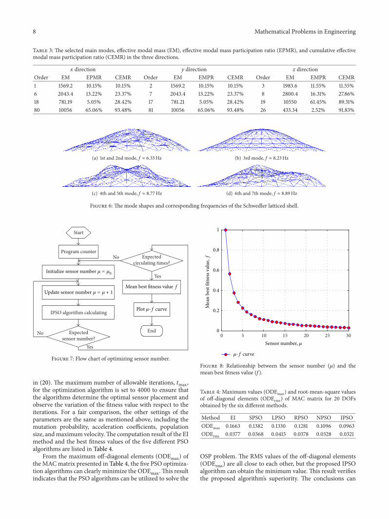
4.3. Sensor Number. The sensor number is one of the keyissues in OSP problems. In this section, the proposed IPSOalgorithm is introduced to search for the best fitness valuewith respect to each sensor number. A circulating compu-tation strategy is adopted to determine the optimal sensornumber and enhance the precision and reliability of thecomputation result. With this strategy, the mean best fitnesscan be obtained. The sensor number is 𝜇, and the meanbest fitness value is 𝑓. Thus, the 𝜇-f curve can be obtained,which indicates the relationship between the sensor numberand the mean best fitness value. In this curve, the stablepoint demonstrates that the fitness does not change or onlyslightly changes with the increase in the sensor number.Therefore, the corresponding sensor number of this point isthe economical one. This computation method’s flow chart isshown in Figure 7.

For each computation, this method calculates the fitnessvalue of each sensor. For each sensor, the IPSO algorithmrepeats the maximum number of allowable iterations tosearch for the best fitness value. Therefore, this approachbecomes complex and time-consuming if the maximumcomputation trial, sensor number, and allowable iterationsare too large. We are also more concerned about the stablepoint of the 𝜇-f curve than the calculating accuracy for thegiven problem. The maximum computation trial is set to 10,the maximum sensor number is set to 30, and the maximumnumber of allowable iterations is set to 100 so as to lower thecomputation complexity. The mutation probability 𝑃𝑚 = 0.4,andmutation step size linearly decreases in the range of [𝑉max,0.1𝑉max]. The acceleration coefficients 𝑐1 = 𝑐2 = 2.0, thepopulation size 𝑁 = 40, and the maximum velocity 𝑉max isequal to the candidate DOFs (i.e., 𝑉max = 363). The obtained𝜇-f curve for the 10 trials can be seen in Figure 8. The meanbest fitness value clearly becomes smaller with the increasein the sensor number. This condition indicates that moreinformation can be obtained withmore sensors placed on thestructures. The decreasing rate of the mean best fitness valuebecomes slow when the number of sensors increases to 20.Thus, we considered 20 as the stable point of the 𝜇-f curveand set the economical sensor number to 20.

4.4. Results of the Contrast Experiments and Analysis. Thecomparison simulations of EI, SPSO, LPSO, NPSO, andRPSO algorithms are conducted to assess the proposedIPSO algorithm’s performance.The inertia weight adjustmentstrategies of the five different PSO algorithms are set asfollows. In SPSO, the inertia weight is fixed at 0.9. In LSPO,the inertia weight linearly decreases from 0.9 to 0.4. InNPSO,the inertia weight nonlinearly decreases from 0.2 to −0.3 withthe slope 𝑚 = −2.5 × 10−4 and exponent 𝛼 = 1.2. In RPSO,the inertia weight changes randomly according to (18). Inthe proposed IPSO, the inertia weight nonlinearly decreasesfrom 0.9 to 0.4 with the exponent 𝑘 = 10 as described


Table 3: The selected main modes, effective modal mass (EM), effective modal mass participation ratio (EPMR), and cumulative effectivemodal mass participation ratio (CEMR) in the three directions.

𝑥 direction 𝑦 direction 𝑧 directionOrder EM EPMR CEMR Order EM EMPR CEMR Order EM EMPR CEMR1 1569.2 10.15% 10.15% 2 1569.2 10.15% 10.15% 3 1983.6 11.55% 11.55%6 2043.4 13.22% 23.37% 7 2043.4 13.22% 23.37% 8 2800.4 16.31% 27.86%18 781.19 5.05% 28.42% 17 781.21 5.05% 28.42% 19 10550 61.45% 89.31%80 10056 65.06% 93.48% 81 10056 65.06% 93.48% 26 433.34 2.52% 91.83%

(a) 1st and 2nd mode, f ≈ 6.33Hz (b) 3rd mode, f ≈ 8.23Hz

(c) 4th and 5th mode, f ≈ 8.77Hz (d) 6th and 7th mode, f ≈ 8.89Hz

Figure 6: The mode shapes and corresponding frequencies of the Schwedler latticed shell.

Program counter

IPSO algorithm calculating

Expectedsensor number?

Expectedcirculating times?

Yes

Yes

No

No

Start

End

Initialize sensor number 𝜇 = 𝜇0

Update sensor number 𝜇 = 𝜇 + 1Mean best fitness value f

Plot 𝜇-f curve

Figure 7: Flow chart of optimizing sensor number.

in (20). The maximum number of allowable iterations, 𝑡max,for the optimization algorithm is set to 4000 to ensure thatthe algorithms determine the optimal sensor placement andobserve the variation of the fitness value with respect to theiterations. For a fair comparison, the other settings of theparameters are the same as mentioned above, including themutation probability, acceleration coefficients, populationsize, andmaximum velocity.The computation result of the EImethod and the best fitness values of the five different PSOalgorithms are listed in Table 4.

From the maximum off-diagonal elements (ODEmax) ofthe MACmatrix presented in Table 4, the five PSO optimiza-tion algorithms can clearly minimize the ODEmax. This resultindicates that the PSO algorithms can be utilized to solve the

0 5 10 15 20 25 30Sensor number, 𝜇

Mea

n be

st fit

ness

val

ue, f

𝜇-f curve

1

0.8

0.6

0.4

0.2

0

Figure 8: Relationship between the sensor number (𝜇) and themean best fitness value (f ).

Table 4: Maximum values (ODEmax) and root-mean-square valuesof off-diagonal elements (ODErms) of MAC matrix for 20 DOFsobtained by the six different methods.

Method EI SPSO LPSO RPSO NPSO IPSOODEmax 0.1663 0.1382 0.1330 0.1281 0.1096 0.0963ODErms 0.0377 0.0368 0.0415 0.0378 0.0328 0.0321

OSP problem. The RMS values of the off-diagonal elements(ODErms) are all close to each other, but the proposed IPSOalgorithm can obtain the minimum value. This result verifiesthe proposed algorithm’s superiority. The conclusions can


1 2 3 4 5 6 7 8 9 10 11 12

1234567891011120

0.2

0.4

0.6

0.8

1

Mode

Mode

MAC

(a)

1 2 3 4 5 6 7 8 9 10 11 12

1234567891011120

0.2

0.4

0.6

0.8

1

Mode

Mode

MAC

(b)

1 2 3 4 5 6 7 8 9 10 11 12

1234567891011120

0.2

0.4

0.6

0.8

1

ModeMode

MAC

(c)

1 2 3 4 5 6 7 8 9 10 11 12

1234567891011120

0.2

0.4

0.6

0.8

1

ModeMode

MAC

(d)

1 2 3 4 5 6 7 8 9 10 11 12

1234567891011120

0.2

0.4

0.6

0.8

1

Mode

Mode

MAC

(e)

1 2 3 4 5 6 7 8 9 10 11 12

1234567891011120

0.2

0.4

0.6

0.8

1

Mode

Mode

MAC

(f)

Figure 9: MAC values of 20 DOFs obtained by the six different methods. (a) EI method. (b) SPSO method. (c) LPSO method. (d) RPSOmethod. (e) NPSO method. (f) IPSO method.


0 500 1000 1500 2000 2500 3000 3500 40000.03

0.04

0.05

0.06

0.07

0.08

0.09

SPSOLPSORPSO

NPSOIPSO

Iteration number, t

Best

fitne

ss v

alue

, f

Figure 10: Performances of the five PSO algorithms.

also be reached from the distribution of theMAC values fromthe six different methods given in Figure 9. All of the off-diagonal elements are intuitionally displayed in this figure.The proposed IPSO algorithm can obtain smaller valuescompared with the other five methods. In Figure 10, the bestfitness values of the five PSO algorithms are compared. TheIPSO algorithm can clearly determine the minimum fitnessamong these optimization algorithms. Finally, the placementresults in three directions of the IPSO algorithm are given inFigure 11.

4.5. Discussion. Thepresentation case is based on the FEMofa latticed shell structure, which is created in strict accordancewith the actual structure. Therefore, the validity of the pro-posed IPSO algorithm and the obtained optimal placementscheme can be verified by the comparison simulation results.However, this study still has some inevitable limitations. Forexample, the IPSO algorithm performance with different 𝑘values is not presented. Thus, the determination of 𝑘 maybe empirical to a certain extent. The FEM errors may alsoimpact the placement results that are not considered in thesimulation experiments. However, this problem could besolved if we consider a sensor placement experiment on a reallatticed shell structure.

5. Conclusions and Future Work

In this paper, a novel IPSO approach is presented to addressthe existing defects of the traditional sensor placementmethods. Firstly, a new method is proposed to select themode number. Three strategies are then adopted to improvethe PSO algorithm. Finally, the proposed IPSO approachis applied to determine the optimal sensor number andlocations. With simulation experiments, some conclusionsare summarized as follows.

Y

XZ

32

59

37

86

80

104

5429

27

132

134

137

121 97

95114

66

45

Figure 11: Optimal placement result of IPSO algorithm.

(1) In selecting the proper modes, a new method calledcumulative effective modal mass participation ratiois proposed, which can reflect the dynamic responseof the given modes. Using this method, the sufficientmain modes can be selected.

(2) Strategies such as the dual-structure coding, novelnonlinear inertia weight adjustment method, andmutation operator can be utilized to improve the PSOalgorithm’s search ability.

(3) The optimal sensor number is determined by a cir-culating computation strategy.Thismethod calculatesthemean best fitness value with the increase in sensornumber. Therefore, the computation result is preciseand reliable.

(4) The contrast simulation results with the EI methodand four different PSO algorithms for a latticed shellstructure show that the proposed IPSO algorithmhas better enhancement in convergence speed andprecision.

The effectiveness of the IPSO approach has been provenin this study through simulation experiments.However, someaspects need to be further studied. The model errors shouldbe investigated in future research.

Conflict of Interests

The authors declare that there is no conflict of interestsregarding the publication of this paper.

References

[1] D. S. Shan, Z. H. Wan, and L. Qiao, “Optimal sensor place-ment for long-span railway steel truss cable-stayed bridge,” inProceedings of the 3rd International Conference on MeasuringTechnology and Mechatronics Automation (ICMTMA ’11), pp.795–798, January 2011.


[2] D. C. Kammer, “Sensor placement for on-orbit modal identi-fication and correlation of large space structures,” Journal ofGuidance, Control, and Dynamics, vol. 14, no. 2, pp. 251–259,1991.

[3] F. E. Udwadia, “Methodology for optimum sensor locationsfor parameter identification in dynamic systems,” Journal ofEngineering Mechanics, vol. 120, no. 2, pp. 368–390, 1994.

[4] D. C. Kammer andM. L. Tinker, “Optimal placement of triaxialaccelerometers for modal vibration tests,” Mechanical Systemsand Signal Processing, vol. 18, no. 1, pp. 29–41, 2004.

[5] M. Meo and G. Zumpano, “On the optimal sensor placementtechniques for a bridge structure,” Engineering Structures, vol.27, no. 10, pp. 1488–1497, 2005.

[6] C. Papadimitriou, “Optimal sensor placement methodologyfor parametric identification of structural systems,” Journal ofSound and Vibration, vol. 278, no. 4-5, pp. 923–947, 2004.

[7] C. Papadimitriou, “Pareto optimal sensor locations for struc-tural identification,” Computer Methods in Applied Mechanicsand Engineering, vol. 194, no. 12–16, pp. 1655–1673, 2005.

[8] I. Trendafilova, W. Heylen, and H. Van Brussel, “Measurementpoint selection in damage detection using the mutual informa-tion concept,” Smart Materials and Structures, vol. 10, no. 3, pp.528–533, 2001.

[9] C. Schedlinski and M. Link, “An approach to optimal pick-upand exciter placement,” Proceeding of SPIE International Societyfor Optical Engineering, pp. 376–382, 1996.

[10] Y. S. Park and H. B. Kim, “Sensor placement guide for modelcomparison and improvement,” Proceeding of SPIE Interna-tional Society For Optical Engineering, pp. 404–409, 1996.

[11] A. P. Cherng, “Optimal sensor placement for modal parameteridentification using signal subspace correlation techniques,”Mechanical Systems and Signal Processing, vol. 17, no. 2, pp. 361–378, 2003.

[12] M. Reynier andH. Abou-Kandil, “Sensors location for updatingproblems,”Mechanical Systems and Signal Processing, vol. 13, no.2, pp. 297–314, 1999.

[13] J. E. T. Penny,M. I. Friswell, and S. D. Garvey, “Automatic choiceof measurement locations for dynamic testing,” AIAA journal,vol. 32, no. 2, pp. 407–414, 1994.

[14] C. B. Larson, D. C. Zimmerman, and E. L. Marek, “A compar-ison of modal test planning techniques: excitation and sensorplacement using the NASA 8-bay truss,” Proceeding of SPIEInternational Society for Optical Engineering, pp. 205–205, 1994.

[15] G. Heo, M. L. Wang, and D. Satpathi, “Optimal transducerplacement for health monitoring of long span bridge,” SoilDynamics and Earthquake Engineering, vol. 16, no. 7-8, pp. 495–502, 1997.

[16] W. Heylen and P. Sas, Modal Analysis Theory and Testing,Departement Werktuigkunde, Katholieke Universteit Leuven,2006.

[17] G. C. Marano, G. Monti, and G. Quaranta, “Comparisonof different optimum criteria for sensor placement in latticetowers,” Structural Design of Tall and Special Buildings, vol. 20,no. 8, pp. 1048–1056, 2011.

[18] L. Yao, W. A. Sethares, and D. C. Kammer, “Sensor placementfor on-orbit modal identification via a genetic algorithm,”AIAAjournal, vol. 31, no. 10, pp. 1922–1928, 1993.

[19] R. R. Brooks, S. S. Iyengar, and J. Chen, “Automatic correlationand calibration of noisy sensor readings using elite geneticalgorithms,” Artificial Intelligence, vol. 84, no. 1-2, pp. 339–354,1996.

[20] W. Liu, W. C. Gao, Y. Sun, and M. J. Xu, “Optimal sensor place-ment for spatial lattice structure based on genetic algorithms,”Journal of Sound and Vibration, vol. 317, no. 1-2, pp. 175–189,2008.

[21] G. Ma, F. L. Huang, and X. M. Wang, “Optimal placementof sensors in monitoring for bridge based on hybrid geneticalgorithm,” Journal of Vibration Engineering, vol. 21, no. 2, pp.191–196, 2008.

[22] K.D.Dhuri and P. Seshu, “Multi-objective optimization of piezoactuator placement and sizing using genetic algorithm,” Journalof Sound and Vibration, vol. 323, no. 3—5, pp. 495–514, 2009.

[23] Y. J. Cha, A. K. Agrawal, Y. Kim, and A. M. Raich, “Multi-objective genetic algorithms for cost-effective distributions ofactuators and sensors in large structures,” Expert Systems withApplications, vol. 39, no. 9, pp. 7822–7833, 2012.

[24] C. He, J. C. Xing, J. L. Li et al., “A combined optimal sensorplacement strategy for the structural health monitoring ofbridge structures,” International Journal of Distributed SensorNetworks, vol. 2013, Article ID 820694, 9 pages, 2013.

[25] A. R.M. Rao andG. Anandakumar, “Optimal placement of sen-sors for structural system identification and health monitoringusing a hybrid swarm intelligence technique,” Smart Materialsand Structures, vol. 16, no. 6, pp. 2658–2672, 2007.

[26] J. J. Lian, L. J. He, B. Ma et al., “Optimal sensor placement forlarge structures using the nearest neighbour index and a hybridswarm intelligence algorithm,” Smart Materials and Structures,vol. 22, no. 9, Article ID 095015, 2013.

[27] L. J. He, J. J. Lian, B. Ma, and H. J. Wang, “Optimal multiaxialsensor placement for modal identification of large structures,”Structural Control and Health Monitoring, vol. 21, no. 1, pp. 61–79, 2014.

[28] R. C. Eberhart and J. Kennedy, “New optimizer using particleswarm theory,” in Proceedings of the 6th International Sympo-sium onMicroMachine and Human Science, pp. 39–43, October1995.

[29] J. Kennedy and R. C. Eberhart, “Particle swarm optimization,”in Proceedings of the IEEE International Conference on NeuralNetworks, pp. 1942–1948, December 1995.

[30] E. L. Wilson,Three-Dimensional Static and Dynamic Analysis ofStructures. Computers and Structures, CSI, Berkeley, Calif, USA,2002.

[31] T. H. Yi, H. N. Li, and M. Gu, “Optimal sensor placementfor health monitoring of high-rise structure based on geneticalgorithm,” Mathematical Problems in Engineering, vol. 2011,Article ID 395101, 12 pages, 2011.

[32] Y. H. Shi and R. C. Eberhart, “A modified particle swarmoptimizer,” in Proceedings of the IEEE International Conferenceon Evolutionary Computation, pp. 69–73, May 1998.

[33] Y. H. Shi and R. C. Eberhart, “Empirical study of particleswarm optimization,” in Proceedings of the IEEE Congress onEvolutionary Computation, pp. 1945–1950, 1999.

[34] R. C. Eberhart andY.H. Shi, “Tracking and optimizing dynamicsystems with particle swarms,” in Proceedings of the Congress onEvolutionary Computation, pp. 94–100, May 2001.

[35] A. Chatterjee and P. Siarry, “Nonlinear inertia weight variationfor dynamic adaptation in particle swarm optimization,” Com-puters and Operations Research, vol. 33, no. 3, pp. 859–871, 2006.

[36] A. Ratnaweera, S. K. Halgamuge, and H. C. Watson, “Self-organizing hierarchical particle swarm optimizer with time-varying acceleration coefficients,” IEEE Transactions on Evolu-tionary Computation, vol. 8, no. 3, pp. 240–255, 2004.


[37] T. G. Carne and C. R. Dohrmann, “Amodal test design strategyfor modal correlation,” Proceeding of SPIE International Societyfor Optical Engineering, pp. 927–927, 1995.

[38] J. Teng and Y. H. Zhu, “Optimal sensor placement for modalparameters test of large span spatial steel structural,” Engineer-ing Mechanics, vol. 28, no. 3, pp. 150–156, 2011 (Chinese).

[39] P. Kohnke, ANSYSTheory Manual, ANSYS Inc, 2001.[40] J. S. Zhang, Y. Wu, and S. Z. Shen, “Identification of natural

modeswith significant contributions towind-induced vibrationof single-layer reticulated shell,” Journal of Vibration Engineer-ing, vol. 19, no. 4, pp. 452–458, 2006 (Chinese).

Submit your manuscripts athttp://www.hindawi.com

Hindawi Publishing Corporationhttp://www.hindawi.com Volume 2014

MathematicsJournal of


Mathematical Problems in Engineering

Hindawi Publishing Corporationhttp://www.hindawi.com

Differential EquationsInternational Journal of

Volume 2014

Applied MathematicsJournal of


Probability and StatisticsHindawi Publishing Corporationhttp://www.hindawi.com Volume 2014

Journal of


Mathematical PhysicsAdvances in

Complex AnalysisJournal of


OptimizationJournal of


CombinatoricsHindawi Publishing Corporationhttp://www.hindawi.com Volume 2014

International Journal of


Operations ResearchAdvances in

Journal of


Function Spaces

Abstract and Applied AnalysisHindawi Publishing Corporationhttp://www.hindawi.com Volume 2014

International Journal of Mathematics and Mathematical Sciences


The Scientific World JournalHindawi Publishing Corporation http://www.hindawi.com Volume 2014


Algebra

Discrete Dynamics in Nature and Society



Decision SciencesAdvances in

Discrete MathematicsJournal of

Hindawi Publishing Corporationhttp://www.hindawi.com

Volume 2014 Hindawi Publishing Corporationhttp://www.hindawi.com Volume 2014

Stochastic AnalysisInternational Journal of

Research Article Optimal Sensor Placement for Latticed...

Documents

Transcript of Research Article Optimal Sensor Placement for Latticed...