Research Article Optimal Rules for Single Machine...
10
Research Article Optimal Rules for Single Machine Scheduling with Stochastic Breakdowns Jinwei Gu, 1 Manzhan Gu, 2,3 and Xingsheng Gu 4 1 School of Economics and Management, Shanghai University of Electric Power, Shanghai 200090, China 2 School of Mathematics, Shanghai University of Finance and Economics, Shanghai 200433, China 3 School of Electrical and Computer Engineering, Georgia Institute of Technology, GA 31407, USA 4 Research Institute of Automation, East China University of Science and Technology, Shanghai 200237, China Correspondence should be addressed to Jinwei Gu; [email protected] Received 2 June 2014; Accepted 4 September 2014; Published 29 September 2014 Academic Editor: Kang Li Copyright © 2014 Jinwei Gu et al. is is an open access article distributed under the Creative Commons Attribution License, which permits unrestricted use, distribution, and reproduction in any medium, provided the original work is properly cited. is paper studies the problem of scheduling a set of jobs on a single machine subject to stochastic breakdowns, where jobs have to be restarted if preemptions occur because of breakdowns. e breakdown process of the machine is independent of the jobs processed on the machine. e processing times required to complete the jobs are constants if no breakdown occurs. e machine uptimes are independently and identically distributed (i.i.d.) and are subject to a uniform distribution. It is proved that the Longest Processing Time first (LPT) rule minimizes the expected makespan. For the large-scale problem, it is also showed that the Shortest Processing Time first (SPT) rule is optimal to minimize the expected total completion times of all jobs. 1. Introduction Machine scheduling problems belong to the classic combina- tional optimization problems. ese problems deal with the model where decision maker needs to arrange jobs to process on a limited number of machines or processors. Machine scheduling problems play an important role in manufac- turing, parallel computing, or compiler optimization. ese problems have been studied since the 1950s and a lot of results have been achieved until now. We refer to the books by Brucker [1] and Pinedo [2] for a general overview of literature in scheduling problems. In the environment of classical scheduling problems, the machine is assumed to be workable continuously until the completion of all jobs. Nevertheless, some unexpected events during production (e.g., equipment damaged, error operation, and instrument breakdown) oſten occur in man- ufacturing environment. erefore, it is very common that a machine breakdown happens during the processing of a job. Moreover, the information about the breakdowns may be uncertain. In the realistic situation, the decision maker has to consider how to utilize the available information to give a more effective scheduling plan in order to increase the output and reduce the cost. In this way, it is necessary and valuable to research the stochastic scheduling problems with random machine breakdowns. According to the impact a machine breakdown exerts to the job being processed, the machine breakdowns could be categorized into two models: preemptive-resume model and preemptive-repeat. In the preemptive-resume model, if a breakdown happens during the processing of a job, the work done prior to the breakdown is not lost, and the job could be resumed when the machine becomes available again. In the preemptive-repeat model, the job has to be reprocessed in its entirety if the machine breakdown occurs before the job is completed. e main purpose of this paper is to study the prob- lem with machine breakdowns of preemptive-repeat model. ere are many results on preemptive-resume model. Such as Glazebrook [3], Birge et al. [4], Mittenthal and Raghavachari [5], Cai and Zhou [6, 7], and Qi et al. [8]. Regarding the preemptive-repeat model, many authors have contributed remarkable achievements. Adiri et al. [9, 10] studied the problems with single breakdown; Cai et al. [11–13] studied Hindawi Publishing Corporation Mathematical Problems in Engineering Volume 2014, Article ID 260415, 9 pages http://dx.doi.org/10.1155/2014/260415
Transcript of Research Article Optimal Rules for Single Machine...
Research ArticleOptimal Rules for Single Machine Scheduling withStochastic Breakdowns
Jinwei Gu1 Manzhan Gu23 and Xingsheng Gu4
1 School of Economics and Management Shanghai University of Electric Power Shanghai 200090 China2 School of Mathematics Shanghai University of Finance and Economics Shanghai 200433 China3 School of Electrical and Computer Engineering Georgia Institute of Technology GA 31407 USA4Research Institute of Automation East China University of Science and Technology Shanghai 200237 China
Correspondence should be addressed to Jinwei Gu gujinwei1982163com
Received 2 June 2014 Accepted 4 September 2014 Published 29 September 2014
Academic Editor Kang Li
Copyright copy 2014 Jinwei Gu et alThis is an open access article distributed under theCreativeCommonsAttribution License whichpermits unrestricted use distribution and reproduction in any medium provided the original work is properly cited
This paper studies the problem of scheduling a set of jobs on a single machine subject to stochastic breakdowns where jobs haveto be restarted if preemptions occur because of breakdowns The breakdown process of the machine is independent of the jobsprocessed on the machine The processing times required to complete the jobs are constants if no breakdown occurs The machineuptimes are independently and identically distributed (iid) and are subject to a uniform distribution It is proved that the LongestProcessing Time first (LPT) rule minimizes the expected makespan For the large-scale problem it is also showed that the ShortestProcessing Time first (SPT) rule is optimal to minimize the expected total completion times of all jobs
1 Introduction
Machine scheduling problems belong to the classic combina-tional optimization problems These problems deal with themodel where decisionmaker needs to arrange jobs to processon a limited number of machines or processors Machinescheduling problems play an important role in manufac-turing parallel computing or compiler optimization Theseproblems have been studied since the 1950s and a lot ofresults have been achieved until nowWe refer to the books byBrucker [1] and Pinedo [2] for a general overview of literaturein scheduling problems
In the environment of classical scheduling problemsthe machine is assumed to be workable continuously untilthe completion of all jobs Nevertheless some unexpectedevents during production (eg equipment damaged erroroperation and instrument breakdown) often occur in man-ufacturing environment Therefore it is very common thata machine breakdown happens during the processing of ajobMoreover the information about the breakdownsmay beuncertain In the realistic situation the decision maker hasto consider how to utilize the available information to give
a more effective scheduling plan in order to increase theoutput and reduce the cost In this way it is necessary andvaluable to research the stochastic scheduling problems withrandom machine breakdowns
According to the impact a machine breakdown exertsto the job being processed the machine breakdowns couldbe categorized into two models preemptive-resume modeland preemptive-repeat In the preemptive-resumemodel if abreakdown happens during the processing of a job the workdone prior to the breakdown is not lost and the job could beresumed when the machine becomes available again In thepreemptive-repeat model the job has to be reprocessed in itsentirety if the machine breakdown occurs before the job iscompleted
The main purpose of this paper is to study the prob-lem with machine breakdowns of preemptive-repeat modelThere aremany results on preemptive-resumemodel Such asGlazebrook [3] Birge et al [4] Mittenthal and Raghavachari[5] Cai and Zhou [6 7] and Qi et al [8] Regarding thepreemptive-repeat model many authors have contributedremarkable achievements Adiri et al [9 10] studied theproblems with single breakdown Cai et al [11ndash13] studied
Hindawi Publishing CorporationMathematical Problems in EngineeringVolume 2014 Article ID 260415 9 pageshttpdxdoiorg1011552014260415
2 Mathematical Problems in Engineering
the problems in which the realizations of processing timesfor a job between breakdowns are the same They referredto this model as the case of without resampling Frostig [14]considered the resampling mechanism in which the repeatedprocessing times of a job are iid between breakdowns Khaliland Dimitrov [15] studied the flow time of a job under thepreemptive-repeat and preemptive-resume models Lee andLin [16] considered the problem where the decision makercan decide whether to activate a maintenance or to leave themachine to run at a slower speed Kasap et al [17] studied theuptime distributions to ensure that the LPT rule minimizesthe expected makespan Tang and Zhao [18] designed anoptimal algorithm for the problem with early and tardypenalties Lee andYu [19] gave algorithms to the problemwiththe objective to minimize the expected weighted completiontimes and expected maximum tardiness
However all the papers reviewed above (except Kasapet al [17]) carry the implicit assumption that the breakdownprocess of the machine is dependent on the job it is pro-cessing With this assumption the problem with machinebreakdowns could be converted to the traditional schedulingproblem without breakdowns see papers [11 12 18]
In this paper the machine breakdowns are subject topreemptive-repeat model and are independent of job itis processing The objective is to minimize the expectedmakespan or expected total completion times of all jobs Forthis problem Adiri et al [9] firstly studied a special case ofa single machine scheduling with only one breakdown andthe machine is assumed to be continuous workable after thebreakdown Subject to this restriction Adiri et al concludedthat the LPT (SPT) rule minimizes the expected makespanwhen the distribution function of the uptime is convex(concave) This paper considers the general problem wherethe downtimes (repairing time) are iid and the uptimesare independently subject to a commonuniformdistributionUnder the assumptions above it is proved that LPT rule isoptimal to achieve the minimal expected makespan and SPTrule minimizes the expected total completion times for large-scale problem where the number of jobs is large enough
The remainder of the paper is organized as followsIn Section 2 the model with stochastic preemptive-repeatbreakdowns is formulatedThen for a given processing orderwe present a formulation of the expected completion timeof a job In Section 3 we show that the LPT rule minimizesthe expectedmakespan Section 4 demonstrates that SPT ruleminimizes the expected total completion times for large-scale problems Finally some concluding remarks are madein Section 5
2 Formulation of Problem
Suppose there are 119899 jobs 1198691 1198692 119869
119899available at time 0
and these jobs are to be processed on a single machineDenote by a constant 119901
119895the time needed to process job
119869119895if no breakdown occurs during its processing Due to
the breakdowns the actual time needed to process job 119869119895
may be more than 119901119895 and the time may vary in different
processing orders It is assumed that the machine could
process one and only one job at a time and once a job beginsto be processed on the machine it could not be preemptedby other jobs (except by machine breakdowns) until itscompletion
The machine is subject to stochastic breakdowns andafter each maintenance the machine will start anew Thebreakdown process is characterized by a sequence of positiverandom vectors 119880
119896 119863119896infin
119896=1 where 119880
119896 119863119896are respectively
the durations of the 119896th uptime and downtime of themachineThe uptimes and downtimes are defined to be inde-pendent of the jobs If the machine breaks down during theprocessing of job 119869
119895 the work done on the job will be lost and
the job has to be restarted 119880119896(119896 = 1 2 ) are defined to be
iid and follow the uniformdistributionwith the distributionfunction 119865(119909) with the support in [0 119862] (0 le 119862 ge sum
119899
119894=1119901119895)
Hence 119865(119909) = 119909119862 (119909 le 119862) 119863119896(119896 = 1 2 ) are also iid
with an arbitrary distribution with E[119863119896] = 1198890 The objective
functions in this paper are the expected makespan and theexpected total completion times Our work focuses on thescheduling order of all jobs so as to minimize the objectivefunctions
Define a jobs processing order 120582 = (1198691 1198692 119869
119899) and
119904119895
= sum119895
119896=1119901119896 (1199040
= 0) Given a processing order 120582 assumethe machine begins to process only the 119895th (119895 + 1)th 119896thjobs at time zero then define that 119862
120582(119895119896)(119896 ge 119895) denotes the
time to complete the 119896 minus 119895 + 1 jobs So the makespan 119862120582
max =
119862120582(1119899)
and the completion time of 119895th job is 119862120582(1119895)
Let 119868119860
be an indicator variable such that 119868119860
= 1 if event A occursotherwise 119868
119860= 0 Based on the notations defined above
the expected completion time of job 119869119895could be expressed
as
E [119862120582(1119895)
] = E[
119895
sum
119896=1
119862120582(1119895)
119868119904119896minus1le1198801lt119904119896
+ 119862120582(1119895)
1198681198801ge119904119895
]
=
119895
sum
119896=1
E [119862120582(1119895)
119868119904119896minus1le1198801lt119904119896
] + E [119862120582(1119895)
1198681198801ge119904119895
]
=
119895
sum
119896=1
Pr (119904119896minus1
le 1198801lt 119904119896)
times E [119862120582(1119895)
| 119904119896minus1
le 1198801lt 119904119896]
+ Pr (1198801ge 119904119895)E [119862
120582(1119895)| 1198801ge 119904119895]
=
119895
sum
119896=1
Pr (119904119896minus1
le 1198801lt 119904119896)
times E [1198801| 119904119896minus1
le 1198801lt 119904119896]
+ 1198890+ E [119862
120582(119896119895)]
+ Pr (1198801ge 119904119895) 119904119895
Mathematical Problems in Engineering 3
=
119895
sum
119896=1
119901119896
119862
[(119904119896minus1
+
119901119896
2
) + 1198890+ E [119862
120582(119896119895)]]
+
119862 minus 119904119895
119862
119904119895
(1)
which implies
E [119862120582(1119895)
] =
1
119862 minus 1199011
119895
sum
119896=2
119901119896[119904119896minus1
+
119901119896
2
+ 1198890+ E [119862
120582(119896119895)]]
+ (119862 minus 119904119895) 119904119895+
1199012
1
2
+ 11988901199011
(2)
Therefore we obtain the expected makespan
E [119862120582
max] = E [119862120582(1119899)
]
=
1
119862 minus 1199011
119899
sum
119896=2
119901119896[119904119896minus1
+
119901119896
2
+ 1198890+ E [119862
120582(119896119899)]]
+ (119862 minus 119904119899) 119904119899+
1199012
1
2
+ 11988901199011
(3)
3 LPT Minimizes Expected Makespan
In this section we will prove the optimality of LPT to mini-mize the expected value of makespan Define the processingorder 120582
119896= (1198691 119869119896minus1
119869119896+1
119869119896 119869119896+2
119869119899) (1 le 119896 le 119899 minus 1)
which is obtained by interchanging the processing order ofthe two jobs 119869
119896 119869119896+1
in 120582 The following lemma shows thatthe processing of first two jobs is subject to LPT rule
Lemma 1 Consider the processing order 120582 = (1198691 1198692 119869
119899) If
the uptimes are iid and uniformly distributed and 1199011
lt 1199012
then the expected makespan can be reduced by interchangingthe first two jobs 119869
1 1198692 that is
E [1198621205821(1119899)
] minus E [119862120582(1119899)
] lt 0 (4)
Proof According to the definition of 119862120582(119895119896)
and by (3) it isobtained that
E [119862120582(2119899)
]
=
1
119862 minus 1199012
119899
sum
119896=3
119901119896[(119904119896minus1
minus 1199011) +
119901119896
2
+ 1198890+ E [119862
120582(119896119899)]]
+ [119862 minus (119904119899minus 1199011)] (119904119899minus 1199011) +
1199012
2
2
+ 11988901199012
(5)
By replacing (5) in (3)
E [119862120582(1119899)
]
=
1
119862 minus 1199011
119899
sum
119896=3
119901119896(119904119896minus1
+
119901119896
2
+ 1198890+ E [119862
120582(119896119899)])
+
1
119862 minus 1199011
[(119862 minus 119904119899) 119904119899+
1199012
1
2
+ 11988901199011]
+
1199012
119862 minus 1199011
(1199041+
1199012
2
+ 1198890)
+
1199012
(119862 minus 1199012) (119862 minus 119901
1)
times [
119899
sum
119896=3
119901119896((119904119896minus1
minus 1199011) +
119901119896
2
+ 1198890+ E [119862
120582(119896119899)])
+ (119862 minus (119904119899minus 1199011)) (119904119899minus 1199011) +
1199012
2
2
+ 11988901199012]
(6)
That is
E [119862120582(1119899)
] =
119862
(119862 minus 1199011) (119862 minus 119901
2)
times
119899
sum
119896=3
119901119896(119904119896minus1
+
119901119896
2
+ 1198890+ E [119862
120582(119896119899)])
minus
11990111199012
(119862 minus 1199011) (119862 minus 119901
2)
119899
sum
119896=3
119901119896
+
1
(119862 minus 1199011) (119862 minus 119901
2)
times (
+211990111199012119904119899+ 1198622119904119899minus 1198621199042
119899
+
1198621199012
1
2
+
1198621199012
2
2
+ 11986211988901199011+ 11986211988901199012
minus119889011990111199012minus 11990111199012
2minus
31199012
11199012
2
)
(7)
By the same method we could get the expression ofE[1198621205821(1119899)
] Since
E [1198621205821(119896119899)
] = E [119862120582(119896119899)
] for 119896 = 3 4 119899 (8)
we obtain
E [1198621205821(1119899)
] minus E [119862120582(1119899)
]
=
1
(119862 minus 1199011) (119862 minus 119901
2)
times [(minus11990121199012
1minus
31199012
21199011
2
) minus (minus11990111199012
2minus
31199012
11199012
2
)]
=
11990111199012
2 (119862 minus 1199011) (119862 minus 119901
2)
(1199011minus 1199012)
(9)
The conclusion follows by 1199011lt 1199012
4 Mathematical Problems in Engineering
Corollary 2 Assume the uptimes are iid and uniformlydistributed If 119901
119896lt 119901119896+1
then
E [119862120582119896(119896119899)
] minus E [119862120582(119896119899)
] lt 0 119891119900119903 1 le 119896 le 119899 minus 1 (10)
Proof The proof is the same as that in Lemma 1
Next we will give another expression for E[119862120582119896(119896119899)
] minus
E[119862120582(119896119899)
] Assume the machine begins to process jobs119869119896 119869119896+1
119869119899at time zero and 119901
119896lt 119901119896+1
Let 1198961
= min119894 |
119880119894ge 119901119896 then we consider the following three cases
Case 1 (119901119896
le 1198801198961
lt 119901119896+1
) With the possibility (119865(119901119896+1
) minus
119865(119901119896))(1 minus 119865(119901
119896)) in this case we have
E [119862120582119896(119896119899)
] minus E [119862120582(119896119899)
] = E [119862120582119896(119896119899)
] minus E [119862120582(119896+1119899)
]
≐ Δ1gt 0
(11)
Case 2 (119901119896+1
le 1198801198961
lt 119901119896+119901119896+1
)With the possibility (119865(119901119896+1
+
119901119896) minus 119865(119901
119896+1))(1 minus 119865(119901
119896)) we have
E [119862120582119896(119896119899)
] minus E [119862120582(119896119899)
] = E [119862120582119896(119896+1119899)
] minus E [119862120582(119896+1119899)
]
≐ Δ2lt 0
(12)
Case 3 (1198801198961
ge 119901119896+ 119901119896+1
) We have
E [119862120582119896(119896119899)
] minus E [119862120582(119896119899)
] = 0 (13)
From the three cases above we get
E [119862120582119896(119896119899)
] minus E [119862120582(119896119899)
] =
119865 (119901119896+1
) minus 119865 (119901119896)
1 minus 119865 (119901119896)
Δ1
+
119865 (119901119896+ 119901119896+1
) minus 119865 (119901119896+1
)
1 minus 119865 (119901119896)
Δ2
(14)
Known from Corollary 2 we know E[119862120582119896(119896119899)
] minus E[119862120582(119896119899)
] lt
0 Hence
119865 (119901119896+1
) minus 119865 (119901119896)
1 minus 119865 (119901119896)
Δ1+
119865 (119901119896+ 119901119896+1
) minus 119865 (119901119896+1
)
1 minus 119865 (119901119896)
Δ2lt 0
(15)
That is
Δ1
Δ2
gt
119901119896
119901119896minus 119901119896+1
(16)
The following lemma shows that the processing of any twoconsecutive jobs is subject to LPT rule
Lemma 3 Assume the uptimes are iid and uniformly dis-tributed If 119901
119896lt 119901119896+1
then
E [119862120582119896(1119899)
] minus E [119862120582(1119899)
] lt 0 119891119900119903 1 lt 119896 le 119899 minus 1 (17)
Proof Let 119880lowast be the uptime where the job 119869119896minus1
is completedand assume the machine has been continuously processingjobs for 119905
lowast time units when 119869119896minus1
is finished at time 1199050 that
is we have 119880lowast
gt 119905lowast Let 119883 = 119880
lowastminus 119905lowast and let 119866(119909) be the
distribution function of 119883 We have
119866 (119909) = Pr (119883 le 119909) = Pr (119880lowast minus 119905lowast
le 119909 | 119880lowast
gt 119905lowast)
=
119909
119862 minus 119905lowast 119909 isin (0 119862 minus 119905
lowast]
(18)
which implies that119883 is uniformly distributed for any given 119905lowast
According to the definition of 119862 we know 119862 minus 119905lowast
ge sum119899
119897=119896119901119897
We now consider four possibilities depending on the value119883
obtains
Case 1 (119883 lt 119901119896) We have
E [119862120582119896(1119899)
] minus E [119862120582(1119899)
] = E [119862120582119896(119896119899)
] minus E [119862120582(119896119899)
] (19)
Case 2 (119901119896le 119883 lt 119901
119896+1) We have
E [119862120582119896(1119899)
] minus E [119862120582(1119899)
] = E [119862120582119896(119896119899)
] minus E [119862120582(119896+1119899)
]
(20)
Case 3 (119901119896+1
le 119883 lt 119901119896+ 119901119896+1
) We have
E [119862120582119896(1119899)
] minus E [119862120582(1119899)
] = E [119862120582119896(119896+1119899)
] minus E [119862120582(119896+1119899)
]
(21)
Case 4 (119883 ge 119901119896+ 119901119896+1
) We have
E [119862120582119896(1119899)
] minus E [119862120582(1119899)
] = 0 (22)
Hence
E [119862120582119896(1119899)
] minus E [119862120582(1119899)
]
= 119866 (119901119896) [E [119862
120582119896(119896119899)] minus E [119862
120582(119896119899)]]
+ [119866 (119901119896+1
) minus 119866 (119901119896)] [E [119862
120582119896(119896119899)] minus E [119862
120582(119896+1119899)]]
+ [119866 (119901119896+ 119901119896+1
) minus 119866 (119901119896+1
)]
times [E [119862120582119896(119896+1119899)
] minus E [119862120582(119896+1119899)
]]
(23)
Because
E [119862120582119896(119896119899)
] minus E [119862120582(119896+1119899)
] = Δ1gt 0
E [119862120582119896(119896+1119899)
] minus E [119862120582(119896+1119899)
] = Δ2lt 0
E [119862120582119896(119896119899)
] minus E [119862120582(119896119899)
] =
119865 (119901119896+1
) minus 119865 (119901119896)
1 minus 119865 (119901119896)
Δ1
+
119865 (119901119896+ 119901119896+1
) minus 119865 (119901119896+1
)
1 minus 119865 (119901119896)
Δ2
(24)
Mathematical Problems in Engineering 5
By replacing (24) in (23) we obtain
E [119862120582119896(1119899)
] minus E [119862120582(1119899)
]
=
119901119896
119862 minus 119905lowast
[
119865 (119901119896+1
) minus 119865 (119901119896)
119865 (119901119896)
Δ1
+
119865 (119901119896+ 119901119896+1
) minus 119865 (119901119896+1
)
119865 (119901119896)
Δ2]
+
119901119896+1
minus 119901119896
119862 minus 119905lowast
Δ1+
119901119896
119862 minus 119905lowastΔ2
=
119862 (119901119896+1
minus 119901119896) Δ2
(119862 minus 119905lowast) (119862 minus 119901
119896)
[
Δ1
Δ2
minus
119901119896
119901119896minus 119901119896+1
]
(25)
By (16) and Δ2lt 0 the conclusion in this lemma holds
Based on Lemmas 1 and 3 the following theorem isimmediate
Theorem 4 Assume the uptimes are iid and uniformlydistributed with support in [0 119862] where 119862 ge sum
119899
119895=1119901119895 then
the LPT rule is optimal to minimize the expected makespan
4 SPT Minimizes Expected TotalCompletion Times
This section considers the single machine problem to min-imize the expected value of total completion times that isE[sum119899
119895=1119862120582(1119895)
] Assume there exist two constants 119901 119901 suchthat119901 le 119901
119895le 119901 for 119895 = 1 2 119899 that is the processing times
of all jobs are uniformly bounded For a given processingorder 120582 if machine begins to process the 119895th (119895+1)th 119896thjobs at time zero define that 120587
120582(119895119896)denotes the sum of the
completion times of the 119896 minus 119895 + 1 jobs So we have
E[
[
119899
sum
119895=1
119862120582(1119895)
]
]
= E [120587120582(1119899)
] (26)
In this section we focus on the large-scale schedulingproblems that is the number of jobs 119899 is large enough Withthe assumption the SPT rule will be proved to be optimal
Lemma 5 Assume the uptimes are iid and uniformly dis-tributed If 119901
1gt 1199012 then
E [1205871205821(1119899)
] minus E [120587120582(1119899)
] lt 0 (27)
for large number 119899
Proof Firstly we have
E [1205871205821(1119899)
] minus E [120587120582(1119899)
] =
119899
sum
119896=1
[E [1198621205821(1119896)
] minus E [119862120582(1119896)
]]
= E [1198621205821(11)
] minus E [119862120582(11)
]
+
119899
sum
119896=2
[E [1198621205821(1119896)
] minus E [119862120582(1119896)
]]
(28)
By (3) we could get the expressions for E[1198621205821(11)
] andE[119862120582(11)
] Hence we obtain
E [1198621205821(11)
] minus E [119862120582(11)
]
= [1199012+
1
119862 minus 1199012
(
1199012
2
2
+ 11988901199012)]
minus [1199011+
1
119862 minus 1199011
(
1199012
1
2
+ 11988901199011)]
=
(1199012minus 1199011)
(119862 minus 1199011) (119862 minus 119901
2)
[1198622minus
119862
2
(1199011+ 1199012) +
11990111199012
2
+ 1198890119862]
(29)
Known from (9) we have
E [1198621205821(1119896)
] minus E [119862120582(1119896)
]
=
(1199012minus 1199011) 11990111199012
2 (119862 minus 1199012) (119862 minus 119901
1)
for 119896 = 2 3 119899
(30)
Therefore we have
E [1205871205821(1119899)
] minus E [120587120582(1119899)
]
=
(1199012minus 1199011)
(119862 minus 1199011) (119862 minus 119901
2)
[1198622minus
119862
2
(1199011+ 1199012) +
11990111199012
2
+ 1198890119862]
+ (119899 minus 1)
(1199012minus 1199011) 11990111199012
2 (119862 minus 1199012) (119862 minus 119901
1)
=
(1199012minus 1199011)
2 (119862 minus 1199012) (119862 minus 119901
1)
[21198622minus 119862 (119901
1+ 1199012minus 21198890)
minus (119899 minus 2) 11990111199012]
(31)
Note 119862 ge sum119899
119895=1119901119895ge 119901119899 so we have 119862
2= Ω(119899
2) and
E [1205871205821(1119899)
minus 120587120582(1119899)
] 997888rarr 1199012minus 1199011 (119899 997888rarr infin) (32)
Since 1199011gt 1199012 we obtain
E [1205871205821(1119899)
] minus E [120587120582(1119899)
] lt 0 (33)
as long as 119899 is large enough
6 Mathematical Problems in Engineering
By Lemma 5 the corollary below follows immediately
Corollary 6 Assume the uptimes are iid and uniformlydistributed If 119901
119896gt 119901119896+1
then
E [120587120582119896(119896119899)
] minus E [120587120582(119896119899)
] lt 0 119891119900119903 1 le 119896 le 119899 minus 1 (34)
as long as 119899 is large enough Also we have
E [120587120582119896(119896119899)
] minus E [120587120582(119896119899)
] =
(119901119896+1
minus 119901119896)
2 (119862 minus 119901119896+1
) (119862 minus 119901119896)
times [21198622minus 119862 (119901
119896+ 119901119896+1
minus 21198890)
minus (119899 minus 119896 minus 1) 119901119896119901119896+1
]
997888rarr 119901119896+1
minus 119901119896 (119899 997888rarr infin)
(35)
Proof The proof is the same as that in Lemma 5
In order to prove the main conclusion in this sectionwe will give another expression for E[120587
120582119896(119896119899)] minus E[120587
120582(119896119899)]
Assume the machine begins to process jobs 119869119896 119869119896+1
119869119899at
time zero and 119901119896
gt 119901119896+1
Let 1198962
= min119894 | 119880119894ge 119901119896+1
and120588 = sum
1198962minus1
119897=1(119880119897+ 119863119897) (120588 = 0 for 119896
2= 1) We consider the
following three cases
Case 1 (119901119896+1
le 1198801198962
lt 119901119896) In this case we have
E [119862120582119896(119896119896)
| 119901119896+1
le 1198801198962
lt 119901119896] = 120588 + 119901
119896+1
E [119862120582119896(119896119897)
| 119901119896+1
le 1198801198962
lt 119901119896]
= 120588 + E [1198801198962
| 119901119896+1
le 1198801198962
lt 119901119896]
+ 1198890+ E [119862
120582119896(119896119897)] 119897 = 119896 + 1 119899
E [119862120582(119896119897)
| 119901119896+1
le 1198801198962
lt 119901119896]
= 120588 + E [1198801198962
| 119901119896+1
le 1198801198962
lt 119901119896]
+ 1198890+ E [119862
120582(119896119897)] 119897 = 119896 119899
(36)
We obtain
E [120587120582119896(119896119899)
minus 120587120582(119896119899)
| 119901119896+1
le 1198801198962
lt 119901119896]
=
119901119896+1
minus 119901119896
2
minus 1198890+ E [120587
120582119896(119896+1119899)]
minus E [120587120582(119896119899)
] ≐ 1205751
(37)
Case 2 (119901119896le 1198801198962
lt 119901119896+ 119901119896+1
) In this case we have
E [119862120582119896(119896119896)
| 119901119896le 1198801198962
lt 119901119896+ 119901119896+1
] = 120588 + 119901119896+1
E [119862120582119896(119896119897)
| 119901119896le 1198801198962
lt 119901119896+ 119901119896+1
]
= 120588 + E [1198801198962
| 119901119896le 1198801198962
lt 119901119896+ 119901119896+1
]
+ 1198890+ E [119862
120582119896(119896119897)] 119897 = 119896 + 1 119899
E [119862120582(119896119896)
| 119901119896le 1198801198962
lt 119901119896+ 119901119896+1
] = 120588 + 119901119896
E [119862120582(119896119897)
| 119901119896le 1198801198962
lt 119901119896+ 119901119896+1
]
= 120588 + E [1198801198962
| 119901119896+1
le 1198801198962
lt 119901119896]
+ 1198890+ E [119862
120582(119896119897)] 119897 = 119896 + 1 119899
(38)
Therefore we get
E [120587120582119896(119896119899)
minus 120587120582(119896119899)
| 119901119896le 1198801198962
lt 119901119896+ 119901119896+1
]
= 119901119896+1
minus 119901119896+ E [120587
120582119896(119896+1119899)] minus E [120587
120582(119896+1119899)] ≐ 1205752
(39)
Case 3 (1198801198962
ge 119901119896+ 119901119896+1
) We have
E [119862120582119896(119896119896)
| 1198801198962
ge 119901119896+ 119901119896+1
] = 120588 + 119901119896+1
E [119862120582(119896119896)
| 1198801198962
ge 119901119896+ 119901119896+1
] = 120588 + 119901119896
E [119862120582119896(119896119897)
| 1198801198962
ge 119901119896+ 119901119896+1
]
= E [119862120582(119896119897)
| 1198801198962
ge 119901119896+ 119901119896+1
] 119897 = 119896 + 1 119899
(40)
And we obtain
E [120587120582119896(119896119899)
minus 120587120582(119896119899)
| 1198801198962
ge 119901119896+ 119901119896+1
] = 119901119896+1
minus 119901119896≐ 1205753lt 0
(41)
Based on the three cases above we have
E [120587120582119896(119896119899)
minus 120587120582(119896119899)
]
= Pr (119901119896+1
le 1198801198962
lt 119901119896| 1198801198962
ge 119901119896+1
) 1205751
+ Pr (119901119896le 1198801198962
lt 119901119896+ 119901119896+1
| 1198801198962
ge 119901119896+1
) 1205752
+ Pr (1198801198962
gt 119901119896+ 119901119896+1
| 1198801198962
ge 119901119896+1
) 1205753
=
1
119862 minus 119901119896+1
[(119901119896minus 119901119896+1
) 1205751+ 119901119896+1
1205752
+ (119862 minus 119901119896minus 119901119896+1
) 1205753] lt 0
(42)
for large number 119899 The inequality holds by the conclusion inCorollary 6
Lemma 7 Assume the uptimes are iid and uniformly dis-tributed If 119901
119896gt 119901119896+1
(1 lt 119896 lt 119899) then one has
E [120587120582119896(1119899)
] minus E [120587120582(1119899)
] lt 0 (43)
for large number 119899
Mathematical Problems in Engineering 7
Proof We let 119880lowast be the uptime where the job 119869
119896minus1is
completed and let 119863lowast be the downtime after 119880lowast Assume the
machine has been continuously processing for 119905lowast time units
when 119869119896minus1
is finished at time 1199050 that is we have 119880
lowastgt 119905lowast Let
119883 = 119880lowastminus 119905lowast and let 119866(119909) be the distribution function of 119883
Here we have
120587120582119896(1119899)
minus 120587120582(1119899)
=
119899
sum
119897=119896
119862120582119896(1119897)
minus
119899
sum
119897=119896
119862120582(1119897)
(44)
Case 1 (119883 lt 119901119896+1
) In this case we have
E [119862120582119896(1119897)
| 119883 lt 119901119896+1
]
= 1199050+ E [119883 | 119883 lt 119901
119896+1] + 1198890+ E [119862
120582119896(119896119897)]
E [119862120582(1119897)
| 119883 lt 119901119896+1
]
= 1199050+ E [119883 | 119883 lt 119901
119896+1] + 1198890+ E [119862
120582(119896119897)]
119897 = 119896 119899
(45)
Therefore we obtain
E [120587120582119896(1119899)
minus 120587120582(1119899)
| 119883 lt 119901119896+1
] = E [120587120582119896(119896119899)
] minus E [120587120582(119896119899)
]
(46)
Case 2 (119901119896+1
le 119883 lt 119901119896) The case is similar to the case 119901
119896+1le
1198801198962
lt 119901119896 So we get
E [120587120582119896(1119899)
minus 120587120582(1119899)
| 119901119896+1
le 119883 lt 119901119896]
=
119901119896+1
minus 119901119896
2
minus 1198890+ E [120587
120582119896(119896+1119899)] minus E [120587
120582(119896119899)] = 1205751
(47)
Case 3 (119901119896
le 119883 lt 119901119896+ 119901119896+1
) The case is similar to the case119901119896le 1198801198962
lt 119901119896+ 119901119896+1
We have
E [120587120582119896(1119899)
minus 120587120582(1119899)
| 119901119896le 119883 lt 119901
119896+ 119901119896+1
]
= 119901119896+1
minus 119901119896+ E [120587
120582119896(119896+1119899)] minus E [120587
120582(119896+1119899)] = 1205752
(48)
Case 4 (119883 ge 119901119896+ 119901119896+1
) The case is similar to the case 1198801198962
ge
119901119896+ 119901119896+1
We obtain
E [120587120582119896(1119899)
minus 120587120582(1119899)
| 119883 ge 119901119896+ 119901119896+1
] = 119901119896+1
minus 119901119896= 1205753
(49)
Based on the four cases above we have
E [120587120582119896(1119899)
minus 120587120582(1119899)
| 119905lowast]
= Pr (119883 lt 119901119896+1
)E [120587120582119896(1119899)
minus 120587120582(1119899)
| 119883 lt 119901119896+1
119905lowast]
+ Pr (119901119896+1
le 119883 lt 119901119896)
times E [120587120582119896(1119899)
minus 120587120582(1119899)
| 119901119896+1
le 119883 lt 119901119896 119905lowast]
+ Pr (119901119896le 119883 lt 119901
119896+ 119901119896+1
)
times E [120587120582119896(1119899)
minus 120587120582(1119899)
| 119901119896le 119883 lt 119901
119896+ 119901119896+1
119905lowast]
+ Pr (119883 gt 119901119896+ 119901119896+1
)
times E [120587120582119896(1119899)
minus 120587120582(1119899)
| 119883 gt 119901119896+ 119901119896+1
119905lowast]
=
119901119896+1
119862 minus 119905lowast
1
119862 minus 119901119896+1
times [(119901119896minus 119901119896+1
) 1205751+ 119901119896+1
1205752+ (119862 minus 119901
119896minus 119901119896+1
) 1205753]
+
119901119896minus 119901119896+1
119862 minus 119905lowast
1205751+
119901119896+1
119862 minus 119905lowast1205752+
119862 minus 119905lowastminus 119901119896minus 119901119896+1
119862 minus 119905lowast
1205753
=
119862
119862 minus 119905lowast
1
119862 minus 119901119896+1
times [(119901119896minus 119901119896+1
) 1205751+ 119901119896+1
1205752+ (119862 minus 119901
119896minus 119901119896+1
) 1205753]
+
minus119905lowast1205753
(119862 minus 119905lowast)
=
119862
119862 minus 119905lowastE [120587120582119896(119896119899)
minus 120587120582(119896119899)
] +
minus119905lowast1205753
(119862 minus 119905lowast)
=
119862
119862 minus 119905lowast
[E [120587120582119896(119896119899)
minus 120587120582(119896119899)
] minus 1205753] + 1205753
(50)
By (35) we have
E [120587120582119896(1119899)
minus 120587120582(1119899)
| 119905lowast]
=
119862
119862 minus 119905lowast
[
1
2 (119862 minus 119901119896+1
) (119862 minus 119901119896)
times (21198622minus 119862 (119901
119896+ 119901119896+1
minus 21198890)
minus (119899 minus 119896 minus 1) 119901119896119901119896+1
) minus 1] sdot 1205753+ 1205753
=
119862
119862 minus 119905lowast
times
119862 (119901119896+ 119901119896+1
) + 21198621198890minus (119899 minus 119896 + 1) 119901
119896119901119896+1
2 (119862 minus 119901119896+1
) (119862 minus 119901119896)
sdot 1205753+ 1205753
(51)
We discuss the following cases
8 Mathematical Problems in Engineering
Case 1 ((119901)2minus 2(119901)
2le 0) Because 119896 gt 1 we have
119896 gt
(119901)2
minus 2(119901)
2
(119901)2
sdot 119899 + 1 (52)
That is
2(119901)
2
119899 minus (119901)2
119899 + 119896(119901)2
minus (119901)2
gt 0 (53)
So we obtain
119862 (119901119896+ 119901119896+1
) + 21198621198890minus (119899 minus 119896 + 1) 119901
119896119901119896+1
ge 2(119901)
2
sdot 119899 minus (119901)2
sdot 119899 + 119896(119901)2
minus (119901)2
gt 0
(54)
Therefore in this case we obtain
E [120587120582119896(1119899)
minus 120587120582(1119899)
| 119905lowast] le 1205753lt 0 (55)
That is
E [120587120582119896(1119899)
minus 120587120582(1119899)
] = E [E [120587120582119896(1119899)
minus 120587120582(1119899)
| 119905lowast]] le 120575
3lt 0
(56)
Case 2 ((119901)2minus 2(119901)
2gt 0) In this case we define 119886 ≐ ((119901)
2minus
2(119901)2)(119901)2 and 0 lt 119886 lt 1 Next two cases are discussed for
the value 119896 obtains
Case 21 (119896 gt 119886 sdot 119899 + 1) In this case we have
119896(119901)2
gt (119901)2
+ [(119901)2
minus 2(119901)
2
] sdot 119899 (57)
That is
2(119901)
2
sdot 119899 minus (119901)2
sdot 119899 + 119896(119901)2
minus (119901)2
gt 0 (58)
Known from Case 1 above we obtain
E [120587120582119896(1119899)
minus 120587120582(1119899)
] le 1205753lt 0 (59)
Case 22 (119896 le 119886 sdot 119899 + 1) According to the definition of 119905lowast wehave 119905
lowastle 119904119896minus1
so
0 lt
119862
119862 minus 119905lowast
le
119862
119862 minus 119904119896minus1
= 1 +
119904119896minus1
119862 minus 119904119896minus1
lt 1 +
119896 sdot 119901
119901119896+ 119901119896+1
+ sdot sdot sdot + 119901119899
lt 1 +
119896
119899 minus 119896
sdot
119901
119901
le 1 +
119886119899 + 1
119899 minus 119886119899 minus 1
sdot
119901
119901
= 1 +
119886 + 1119899
1 minus 119886 minus 1119899
sdot
119901
119901
(60)
Note that there exists a number 119873 such that 1119899 le (1 minus
119886)2 forall119899 gt 119873 so we get
119862
119862 minus 119905lowast
lt 1 +
1 + 119886
1 minus 119886
sdot
119901
119901(61)
for all 119899 gt 119873 Therefore
E [120587120582119896(1119899)
minus 120587120582(1119899)
| 119905lowast]
=
119862
119862 minus 119905lowast
[E [120587120582119896(119896119899)
minus 120587120582(119896119899)
] minus 1205753] + 1205753
le [1 +
1 + 119886
1 minus 119886
sdot
119901
119901
] [E [120587120582119896(119896119899)
minus 120587120582(119896119899)
] minus 1205753] + 1205753
(62)
for all 119899 gt 119873 So we obtain
E [120587120582119896(1119899)
minus 120587120582(1119899)
]
= E [E [120587120582119896(1119899)
minus 120587120582(1119899)
| 119905lowast]]
le [1 +
1 + 119886
1 minus 119886
sdot
119901
119901
] E [120587120582119896(119896119899)
minus 120587120582(119896119899)
] minus 1205753 + 1205753
997888rarr 1205753lt 0 (119899 997888rarr infin)
(63)
Either (119901)2minus 2(119901)
2gt 0 or not we always have
E [120587120582119896(1119899)
minus 120587120582(1119899)
] lt 0 (64)
for large number 119899
Based on Lemmas 5 and 7 the following theorem isimmediate
Theorem 8 Assume the uptimes are iid and uniformlydistributed with support [0 119862] where 119862 ge sum
119899
119894=1119901119894 then the
SPT rule is optimal to minimize the expected value of totalcompletion times if the number of jobs 119899 is large enough
5 Concluding Remarks
The stochastic scheduling problem on a single machine withrandom breakdowns has been investigated in this paperWe consider the situation where the uptimes are uniformlydistributed and iid the downtimes are also assumed tobe iid and follow an arbitrary distribution The machinebreakdowns are defined to be independent of the job it isprocessing Under the assumptions above we prove that (1)the LPT rule could achieve the minimal expected makespan(2) the SPT rule is optimal to minimize the expected valueof total completion times for large scale problems For thescheduling with stochastic breakdowns independent of jobit is processing the result obtained in this paper is thefoundation in this area
Someproblemsmay be considered for the future research(a) whether optimal rule exists when the uptimes are subjectto other probability distributions (b) problems with otherobjective functions are worth investigation (c) the multima-chine version will also be an interesting but difficult problemin the future
Conflict of Interests
The authors declare that there is no conflict of interestsregarding the publication of this paper
Mathematical Problems in Engineering 9
Acknowledgments
We are grateful to the anonymous referees for their valuablecomments and suggestions This research is supported bythe Young Scientists Fund of the National Natural ScienceFoundation of China (61304209 and 11201282) the Fund ofscheme for training young teachers in Colleges and universi-ties in Shanghai (ZZCD12006) the Ministry of Education ofHumanities and Social Science Fund Project (10YJCZH032)and Innovation Program of Shanghai Municipal EducationCommission (14YZ127)
References
[1] P Brucker Scheduling Algorithms Springer 4th edition 2004[2] M Pinedo Scheduling Theory Algorithms and Systems
Springer Heidelberg Germany 3rd edition 2002[3] K D Glazebrook ldquoEvaluating the effects of machine break-
downs in stochastic scheduling problemsrdquo Naval ResearchLogistics vol 34 no 3 pp 319ndash335 1987
[4] J Birge J B G Frenk J Mittenthal and A H G Rinnooy KanldquoSingle-machine scheduling subject to stochastic breakdownsrdquoNaval Research Logistics vol 37 no 5 pp 661ndash677 1990
[5] J Mittenthal and M Raghavachari ldquoStochastic single machinescheduling with quadratic early-tardy penaltiesrdquo OperationsResearch vol 41 no 4 pp 786ndash796 1993
[6] X Cai and X Zhou ldquoAsymmetric earliness and tardinessscheduling with exponential processing times on an unreliablemachinerdquo Annals of Operations Research vol 98 pp 313ndash3312000
[7] X Cai and S Zhou ldquoStochastic scheduling on parallel machinessubject to random breakdowns to minimize expected costs forearliness and tardy jobsrdquo Operations Research vol 47 no 3 pp422ndash437 1999
[8] X D Qi G Yin and J R Birge ldquoSingle-machine schedulingwith randommachine breakdowns and randomly compressibleprocessing timesrdquo Stochastic Analysis and Applications vol 18no 4 pp 635ndash653 2000
[9] I Adiri J Bruno E Frostig and A H G Rinnooy Kan ldquoSinglemachine flow-time scheduling with a single breakdownrdquo ActaInformatica vol 26 no 7 pp 679ndash696 1989
[10] I Adiri E Frostig and A H G Rinnooy Kan ldquoScheduling ona single machine with a single breakdown to minimize stochas-tically the number of tardy jobsrdquo Naval Research Logistics vol38 no 2 pp 261ndash271 1991
[11] X Cai X Sun and X Zhou ldquoStochastic scheduling withpreemptive-repeat machine breakdowns to minimize theexpected weighted flow timerdquo Probability in the Engineering andInformational Sciences vol 17 no 4 pp 467ndash485 2003
[12] X Cai X Sun and X Zhou ldquoStochastic scheduling subjectto machine breakdowns the preemptive-repeat model withdiscounted reward and other criteriardquo Naval Research Logisticsvol 51 no 6 pp 800ndash817 2004
[13] X Cai X Wu and X Zhou ldquoDynamically optimal policiesfor stochastic scheduling subject to preemptive-repeat machinebreakdownsrdquo IEEE Transactions on Automation Science andEngineering vol 2 no 2 pp 158ndash172 2005
[14] E Frostig ldquoA note on stochastic scheduling on a single machinesubject to breakdownmdashthe preemptive repeat modelrdquo Probabil-ity in the Engineering and Informational Sciences vol 5 no 3 pp349ndash354 1991
[15] Z Khalil and B Dimitrov ldquoThe service time properties ofan unreliable server characterize the exponential distributionrdquoAdvances in Applied Probability vol 26 no 1 pp 172ndash182 1994
[16] C Y Lee and C S Lin ldquoSingle-machine scheduling withmaintenance and repair rate-modifying activitiesrdquo EuropeanJournal ofOperational Research vol 135 no 3 pp 493ndash513 2001
[17] N Kasap H Aytug and A Paul ldquoMinimizing makespan ona single machine subject to random breakdownsrdquo OperationsResearch Letters vol 34 no 1 pp 29ndash36 2006
[18] H Tang and C Zhao ldquoStochastic single machine schedulingsubject to machines breakdowns with quadratic early-tardypenalties for the preemptive-repeat modelrdquo Journal of AppliedMathematics and Computing vol 25 no 1-2 pp 183ndash199 2007
[19] C Y Lee andG Yu ldquoSinglemachine scheduling under potentialdisruptionrdquo Operations Research Letters vol 35 no 4 pp 541ndash548 2007
Submit your manuscripts athttpwwwhindawicom
Hindawi Publishing Corporationhttpwwwhindawicom Volume 2014
MathematicsJournal of
Hindawi Publishing Corporationhttpwwwhindawicom Volume 2014
Mathematical Problems in Engineering
Hindawi Publishing Corporationhttpwwwhindawicom
Differential EquationsInternational Journal of
Volume 2014
Applied MathematicsJournal of
Hindawi Publishing Corporationhttpwwwhindawicom Volume 2014
Probability and StatisticsHindawi Publishing Corporationhttpwwwhindawicom Volume 2014
Journal of
Hindawi Publishing Corporationhttpwwwhindawicom Volume 2014
Mathematical PhysicsAdvances in
Complex AnalysisJournal of
Hindawi Publishing Corporationhttpwwwhindawicom Volume 2014
OptimizationJournal of
Hindawi Publishing Corporationhttpwwwhindawicom Volume 2014
CombinatoricsHindawi Publishing Corporationhttpwwwhindawicom Volume 2014
International Journal of
Hindawi Publishing Corporationhttpwwwhindawicom Volume 2014
Operations ResearchAdvances in
Journal of
Hindawi Publishing Corporationhttpwwwhindawicom Volume 2014
Function Spaces
Abstract and Applied AnalysisHindawi Publishing Corporationhttpwwwhindawicom Volume 2014
International Journal of Mathematics and Mathematical Sciences
Hindawi Publishing Corporationhttpwwwhindawicom Volume 2014
The Scientific World JournalHindawi Publishing Corporation httpwwwhindawicom Volume 2014
Hindawi Publishing Corporationhttpwwwhindawicom Volume 2014
Algebra
Discrete Dynamics in Nature and Society
Hindawi Publishing Corporationhttpwwwhindawicom Volume 2014
Hindawi Publishing Corporationhttpwwwhindawicom Volume 2014
Decision SciencesAdvances in
Discrete MathematicsJournal of
Hindawi Publishing Corporationhttpwwwhindawicom
Volume 2014 Hindawi Publishing Corporationhttpwwwhindawicom Volume 2014
Stochastic AnalysisInternational Journal of
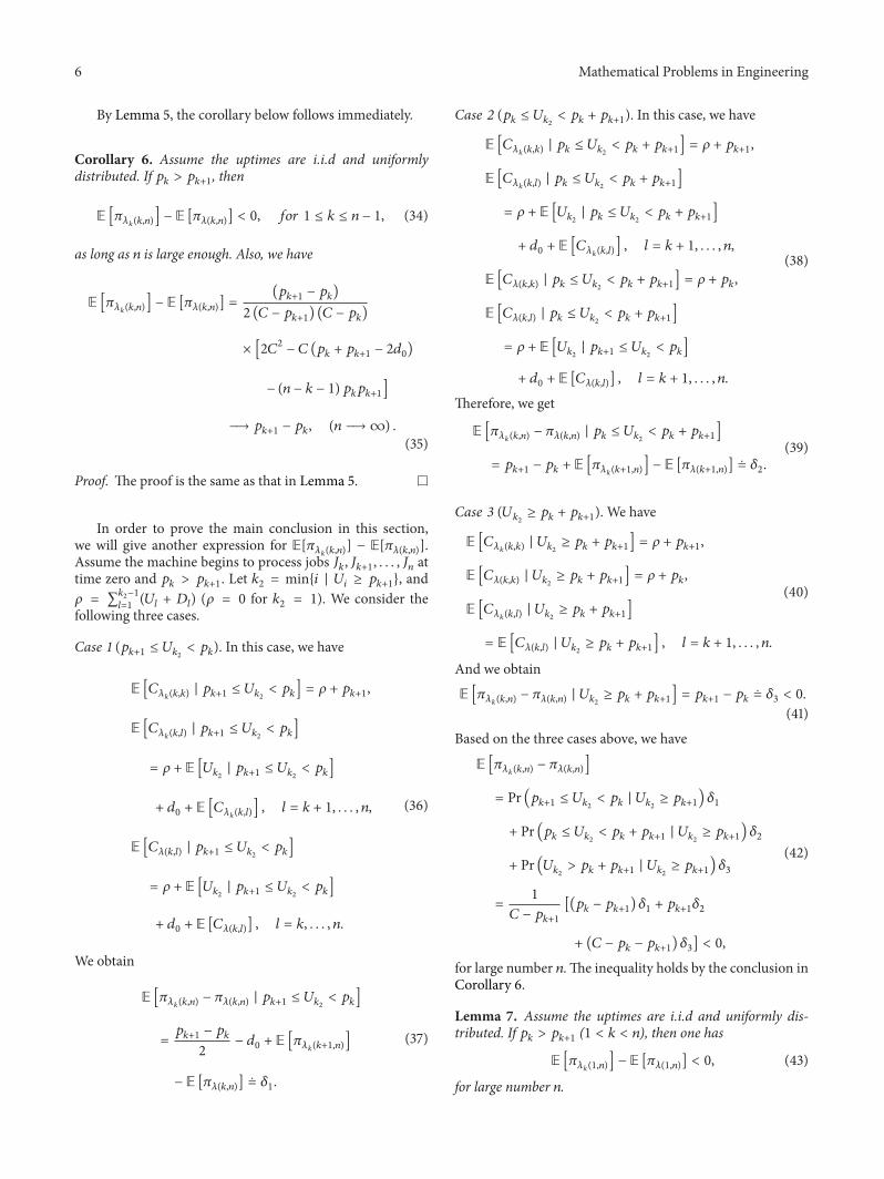