Research Article On the Singular Perturbations for...
10
Research Article On the Singular Perturbations for Fractional Differential Equation Abdon Atangana Institute for Groundwater Studies, Faculty of Natural and Agricultural Sciences, University of the Free State, Bloemfontein 9301, South Africa Correspondence should be addressed to Abdon Atangana; [email protected] Received 29 August 2013; Accepted 19 December 2013; Published 9 February 2014 Academic Editors: R. Bera and Q. Xie Copyright © 2014 Abdon Atangana. is is an open access article distributed under the Creative Commons Attribution License, which permits unrestricted use, distribution, and reproduction in any medium, provided the original work is properly cited. e goal of this paper is to examine the possible extension of the singular perturbation differential equation to the concept of fractional order derivative. To achieve this, we presented a review of the concept of fractional calculus. We make use of the Laplace transform operator to derive exact solution of singular perturbation fractional linear differential equations. We make use of the methodology of three analytical methods to present exact and approximate solution of the singular perturbation fractional, nonlinear, nonhomogeneous differential equation. ese methods are including the regular perturbation method, the new development of the variational iteration method, and the homotopy decomposition method. 1. Introduction Singular perturbation problems have constantly been playing an outstanding character in cooperation in the theory of differential equations and in their applications to the physical world. With a loose knot speaking, singularly perturbed differential equations are pigeonholed by the presence of quite a lot of essentially different scales. e existence of these scales gives one a small parameter and thus permits one to use perturbation methods. It is, however, typical of singular per- turbation problems that a straight forward perturbation fails to be uniformly valid. Traditionally, this type of behaviour, which is abundant in applications, has been tackled by a large variety of methods, such as matched asymptotic expansions and averaging. Nevertheless, many fundamental issues still remain unresolved. Singular perturbation theory is a rich and ongoing area of exploration for mathematicians, physicists, and other researchers. e methods used to tackle problems in this field are many. e more basic of these include the method of matched asymptotic expansions [1–4] and WKB approximation for spatial problems [5–7], and in time, the Poincar´ e-Lindstedt method [8, 9], the method of multiple scales [10, 11], and periodic averaging [12, 13]. While searching in the literature, it is observed that attention has not been paid to the extension of this class of ordinary and partial differential equations to the concept of fractional calculus. In order to accommodate readers that are not acquainted with the concept of fractional calculus, it is perhaps important to recall that fractional calculus, the art of noninteger order integrals and derivatives, has gained an interesting momentum in recent years [14–20]. e applications are ranging from pure and applied mathematics. It is easy to find experts working in this field because of its beauty, while others look for applications. e main aim of this work is to provide impetus, motivation, and to bring together researchers and scientists working in the fields of fractional calculus and perturbation method by providing some useful analytical techniques to derive exact and approximate solutions of this class of equations. e general singular perturbation fractional differential equation considered in this paper is given as follows: () + () + () = () , () = () , () = ℎ () , (1) where ∈ [, ], , and are linear and nonlinear operators, respectively, is the fractional order derivative, is known function, and is a small parameter. We will present the review of the fractional calculus in the next section. Hindawi Publishing Corporation e Scientific World Journal Volume 2014, Article ID 752371, 9 pages http://dx.doi.org/10.1155/2014/752371
Transcript of Research Article On the Singular Perturbations for...
Research ArticleOn the Singular Perturbations for FractionalDifferential Equation
Abdon Atangana
Institute for Groundwater Studies Faculty of Natural and Agricultural Sciences University of the Free StateBloemfontein 9301 South Africa
Correspondence should be addressed to Abdon Atangana abdonatanganayahoofr
Received 29 August 2013 Accepted 19 December 2013 Published 9 February 2014
Academic Editors R Bera and Q Xie
Copyright copy 2014 Abdon Atangana This is an open access article distributed under the Creative Commons Attribution Licensewhich permits unrestricted use distribution and reproduction in any medium provided the original work is properly cited
The goal of this paper is to examine the possible extension of the singular perturbation differential equation to the concept offractional order derivative To achieve this we presented a review of the concept of fractional calculus We make use of theLaplace transform operator to derive exact solution of singular perturbation fractional linear differential equations We makeuse of the methodology of three analytical methods to present exact and approximate solution of the singular perturbationfractional nonlinear nonhomogeneous differential equation These methods are including the regular perturbation method thenew development of the variational iteration method and the homotopy decomposition method
1 Introduction
Singular perturbation problems have constantly been playingan outstanding character in cooperation in the theory ofdifferential equations and in their applications to the physicalworld With a loose knot speaking singularly perturbeddifferential equations are pigeonholed by the presence ofquite a lot of essentially different scalesThe existence of thesescales gives one a small parameter and thus permits one to useperturbation methods It is however typical of singular per-turbation problems that a straight forward perturbation failsto be uniformly valid Traditionally this type of behaviourwhich is abundant in applications has been tackled by a largevariety of methods such as matched asymptotic expansionsand averaging Nevertheless many fundamental issues stillremain unresolved Singular perturbation theory is a rich andongoing area of exploration for mathematicians physicistsand other researchers The methods used to tackle problemsin this field are many The more basic of these include themethod of matched asymptotic expansions [1ndash4] and WKBapproximation for spatial problems [5ndash7] and in time thePoincare-Lindstedt method [8 9] the method of multiplescales [10 11] and periodic averaging [12 13]
While searching in the literature it is observed thatattention has not been paid to the extension of this class of
ordinary and partial differential equations to the concept offractional calculus In order to accommodate readers thatare not acquainted with the concept of fractional calculusit is perhaps important to recall that fractional calculusthe art of noninteger order integrals and derivatives hasgained an interestingmomentum in recent years [14ndash20]Theapplications are ranging from pure and applied mathematicsIt is easy to find experts working in this field because ofits beauty while others look for applications The mainaim of this work is to provide impetus motivation andto bring together researchers and scientists working in thefields of fractional calculus and perturbation method byproviding some useful analytical techniques to derive exactand approximate solutions of this class of equations Thegeneral singular perturbation fractional differential equationconsidered in this paper is given as follows
119863120572
119905119906 (119905) + 120576119860119906 (119905) + 119861119906 (119905) = 119891
120576(119905)
119906 (119886) = 119892 (120576) 119906 (119887) = ℎ (120576)
(1)
where 119905 isin [119886 119887] 119860 and 119861 are linear and nonlinear operatorsrespectively119863120572
119905is the fractional order derivative 119891 is known
function and 120576 is a small parameter We will present thereview of the fractional calculus in the next section
Hindawi Publishing Corporatione Scientific World JournalVolume 2014 Article ID 752371 9 pageshttpdxdoiorg1011552014752371
2 The Scientific World Journal
2 Review of Fractional Calculus
A significant tip is that the fractional derivative at a point 119909 isa local property only when 119886 is an integer in noninteger caseswe cannot say that the fractional derivative at 119909 of a function119891 depends only on values of 119891 very near 119909 in the way thatinteger-power derivatives unquestionably do For that reasonit is anticipated that the philosophy involves some class ofboundary conditions involving information on the functionfurther out To use a metaphor the fractional derivativerequires some tangentialvision As far as the existence of sucha philosophy is concerned the brass tacks of the subject werelaid by Liouville in a paper from 1832
21 Definitions
Definition 1 (Riemann-Liouville integral) The classical formof fractional calculus is given by the Riemann-Liouville inte-gral The theory for periodic functions therefore includingthe ldquoboundary conditionrdquo of repeating after a period is theWeyl integral The Riemann-Liouville integral of order 120572 of afunction 119891(119909) is given by
119886119863minus120572
119905119891 (119909) =
119886119868120572
119905119891 (119909) =
1
Γ (120572)int
119909
119886
(119909 minus 119905)120572minus1
119891 (119905) 119889119905 (2)
Definition 2 (Hadamard fractional integral) The Hadamardfractional integral is introduced by Hadamard [21] and isgiven by the following formula
119886119863minus120572
119905119891 (119909) =
1
Γ (120572)int
119909
119886
(log( 119905
2))
120572minus1119891 (119905)
119905119889119905 (3)
Definition 3 (Riemann-Liouville fractional derivative) Thecorresponding derivative is calculated using Lagrangersquos rulefor differential operators Computing 119899th order derivativeover the integral of order (119899 minus 120572) the 120572 order derivative isobtained It is important to remark that 119899 is the nearest integerbigger than 120572 Not in the same line of ideas like in the caseof classical Newtonian derivatives a fractional derivative isdefined via a fractional integral as follows
119886119863120572
119905119891 (119909) =
119889119899
[119886119868119899
119905119891 (119909)]
119889119909119899
=1
Γ (119899 minus 120572)
119889119899
119889119909119899int
119909
119886
(119909 minus 119905)120572minus1
119891 (119905) 119889119905
(4)
Definition 4 (Caputo fractional derivative) There is anotheralternative for computing fractional derivatives that is theCaputo fractional derivative It was introduced by Caputoand Michel in his 1967 paper [22] In contrast to theRiemann-Liouville fractional derivative when solving differ-ential equations using Caputorsquos definition it is not necessaryto define the fractional order initial conditions Caputorsquosdefinition is illustrated as follows
119862
0119863120572
119905119891 (119909)
=1
Γ (119899 minus 120572)int
119909
119886
(119909 minus 119905)120572minus1
119889119899
119889119905119899119891 (119905) 119889119905
(5)
The above definitions are commonly used in pure and appliedmathematics
Definition 5 If we make use of the primary definition ofan integral as being the antiderivative it would be perhapstempting to propose another definition of fractional deriva-tive which would consist of replacing 120572 by minus120572 in right handof (2) as follows
119886119863120572
119905119891 (119909) =
1
Γ (120572)int
119909
119886
(119909 minus 119905)minus120572minus1
119891 (119905) 119889119905 (6)
The above expression is much simpler to handle on onehand on the other hand it is representing only with a singleintegral The function in this case does not need to be dif-ferentiable in order to compute its fractional derivative Notethat the properties of this derivative will not be presented inthis present work
Definition 6 The Laplace transform is a widely used integraltransformwithmany applications in physics and engineeringThe Laplace transform of the function119891 is defined as follows
L (119891 (119909)) (119904) = int
infin
0
119890minus119904119909
119891 (119909) 119889119909 (7)
22 Properties of Fractional Calculus Two properties of theLaplace transform can be used to define the fractional integraloperator as follows
L (119868 (119891)) = L(int
119909
0
119891 (120591) 119889120591) (119904)
=1
119904L (119891 (119909)) (119904)
L (1198682
(119891)) = L(int
119909
0
int
1199091
0
119891 (120591) 119889120591 1198891199091) (119904)
=1
1199042L (119891 (119909)) (119904)
(8)
Now using the induction method we arrive at the following
L (119868119899
(119891)) =1
119904119899L (119891 (119909)) (119904) (9)
From the above equation we can obtain the following
L (119868119899
(119891)) =1
119904119899L (119891 (119909)) (119904)
997904rArr 119868119899
(119891) = Lminus1
(1
119904119899L (119891 (119909)) (119904))
(10)
It is well-known from the convolution theorem of the Laplacetransform that
L (119891 lowast 119892 (119909)) (119904) = L (119891 (119909)) (119904) sdotL (119892 (119909)) (119904) (11)
The Scientific World Journal 3
Now from the previous formula if we chose for 119892(119909) = 119909120572minus1
with the information of (10) the fractional integral operatorcan be defined as follows
119886119863120572
119905119891 (119909) =
1
Γ (120572)Lminus1
(L (119891 (119909)) (119904) sdotL (119892 (119909)) (119904))
119886119863120572
119905119891 (119909) =
1
Γ (120572)(119891 lowast 119892 (119909)) =
1
Γ (120572)int
119909
119886
(119909 minus 119905)120572minus1
119891 (119905) 119889119905
(12)
According to the classical Newtonian derivative the Leibnizrule is given as
119889119899
[119891 sdot 119892]
119889119909119899=
119899
sum
119896=0
(119899
119896)119891(119896)
(119909) 119892119899minus119896
(119909) (13)
Not in the same line of idea like in the case of classicalNewtonian derivatives the Leibniz rule for the fractionalderivative is given as follows
119886119863120572
119905(119891 (119909) 119892 (119909))
=
119899
sum
119896=0
(119901
119896)119892(119896)
(119909)119886119863119901minus119896
119905119891 (119909)
minus1
119899Γ (minus119901)int
119909
0
(119909 minus 119905)minus119901minus1
119891 (119905) 119889119905
times int
119909
119905
119892119899+1
(120595) (119905 minus 120595)119899
119889120595
(14)
The above result is achieved using a simple integration bypart Now if in addition the functions119891 and 119892 are continuoustogether with their entire derivative on [0 119909] then
lim119899rarrinfin
1
119899Γ (minus119901)int
119909
0
(119909 minus 119905)minus119901minus1
119891 (119905) 119889119905
times int
119909
119905
119892119899+1
(120595) (119905 minus 120595)119899
119889120595 = 0
(15)
In that case we have the following Leibniz rule for fractionalderivative
119886119863120572
119905(119891 (119909) 119892 (119909)) =
119899
sum
119896=0
(119901
119896)119892(119896)
(119909)119886119863119901minus119896
119905119891 (119909) (16)
Let us observe that Laplace transformof the fractional deriva-tive with both Riemann-Liouville and Caputo as follows
L (119862
0119863120572
119905119891 (119909)) (119904) = 119904
120572
119865 (119904) minus
119899minus1
sum
119896=0
119904120572minus119896minus1
119891(119896)
(0)
(119899 minus 1 lt 120572 le 119899)
(17)
The above use the usual initial conditions or values of thefunctions On the other hand we have the Riemann-Liouvillesuch that
L (0119863120572
119905119891 (119909)) (119904) = 119904
120572
119865 (119904) minus
119899minus1
sum
119896=0
119904120572minus119896minus1
119886119863119901minus119896minus1
119905119891 (0)
(119899 minus 1 le 120572 lt 119899)
(18)
The abovemakes use of the unusual initial value or conditionsof the function therefore it is not suitable for the real worldproblems
3 Analytical Methods
In this section make use of some existing analytical methodsto present the exact and approximate solution of some singu-lar perturbation fractional equation (1) It is very importantto note that if the nonlinear term in (1) is zero then it isstraightforward to derive the exact solution of (1) using theLaplace transforms method as follows
31 Laplace Transform Method The first step in this methodconsists of applying the Laplace transform on both sites ofequation to obtain for the case of Caputo derivative as follows
119904120572
119880 (119904) minus
119899minus1
sum
119896=0
119904120572minus119896minus1
119906(119896)
(0) + 120576119860 (119880 (119904)) = 119865120576(119904) (19)
For simplicity we assume that the linear part of the transfor-mation can be written as follows
119860 (119880 (119904)) = 119880 (119904)
119899minus1
sum
119896=0
119892119896(119904 120576) minus ℎ (119904 120576) (20)
We can factorize the term with 119880(119904 120576) then solving 119880(119904 120576)we obtain
119880 (119904 120576) =119865120576(119904) + sum
119899minus1
119896=0119904120572minus119896minus1
119906(119896)
(0) + ℎ (119904 120576)
sum119899minus1
119896=0119892119896(119904 120576) + 119904120572
(21)
Under the condition that the right hand side of the aboveequation is Laplace invertible then we obtain the exactsolution of (1) as follows
119906 (119909 120576) = Lminus1
(119865120576(119904) + sum
119899minus1
119896=0119904120572minus119896minus1
119906(119896)
(0) + ℎ (119904 120576)
sum119899minus1
119896=0119892119896(119904 120576) + 119904120572
)
(22)
In case that the nonlinear part is different to zero otheranalytical methods in this area have been proposed
32TheRegular PerturbationMethod There are several exist-ing perturbation methods for instance match asymptoticexpansion WKB method the multiple-scale analysis andregular perturbation methods [23ndash26] The regular pertur-bation method is perhaps the most naive way to try to solveproblem (1) and this consists of assuming an expansion of thePoincare type as follows
119906 (119909 120576) =
infin
sum
119899=0
119906119899(119909) 120576119899
(23)
On substituting the above in problem (1) one obtains asequence as follows
1198750 119872(119906
0 0) = 0
1198751 1198721(1199060 1199061 0) = 0
119875119899 119872119899(1199060 1199061 1199062 119906
119899) = 0
(24)
4 The Scientific World Journal
The above method has some limitations for instance thenonlinear part can be very difficult to handle for stronglinearity like 119906
119899 119899 ge 3 also the 119872119899(1199060 1199061 1199062 119906
119899) = 0
can also be very difficult to solve Both regular and singularperturbation theory are frequently used in physics and engi-neering Perturbation theory can fail when the system cantransition to a different phase of matter with a qualitativelydifferent behavior that cannot be modeled by the physicalformulas put into the perturbation theory for instance a solidcrystal melting into a liquid In some cases this failure man-ifests itself by divergent behavior of the perturbation seriesSuch divergent series can sometimes be resumed using tech-niques such as Borel resummation However perturbationtechniques can be also used to find approximate solutions tononlinear differential equations Examples of techniques usedto find approximate solutions to these types of problems arethe Lindstedt-Poincare technique the method of harmonicbalancing and the method of multiple time scales
33 Some Iteration Methods Many iterations methods havebeen proposed in the literature so far Some of them providepowerful tools to handle nonlinear and linear equationsranging from ordinary derivatives to fractional derivativesThese techniques are namely the homotopy perturbationmethods (HPM) [27] the homotopy decomposition method[28ndash30] the Adomian decomposition method [31 32] thevariational iteration method [33 34] and the Bernsteincollateral method [35] These mentioned methods have beenused to handle many problems across the sciences In somecases the above iterations produce the exact solutions andalso approximate solutions for strong nonlinear equations
4 Applications
This section is devoted to the discussion underpinning theapplication of Laplace and iteration method for solving sin-gular linear and nonlinear perturbation fractional differentialequation
41 Application of Laplace Transform Linear Case
Example 7 Wewill consider the following singular perturba-tion fractional differential equation
119862
0119863120572
119905119906 (119905) + 120576
119889119906 (119905)
119889119905+ 119905
1198892
119906 (119905)
1198891199052+
119889119906 (119905)
119889119905
=
2120576 (119890minus11990521205762
(minus1 + 120576 (minus1 + 21199052
120576)))
radic120587minus
1199051minus120572
radic120587
times (Hyper geometric PFQ
times ((1
2 1) (1 minus
120572
23
2minus
120572
2 1 minus 119905
2
1205762
)))
(25)
To solve the above equation we apply the Laplace transformon both sides of (25) to obtain
119904120572
119880 (119904) minus 119904120572minus1
119906 (0) + (120576 + 1) (119904119880 (119904) minus 119906 (0))
+L(1199051198892
119906 (119905)
1198891199052) = 119865
120576(119904)
(26)
Here the term is
L(1199051198892
119906 (119905)
1198891199052) = minus
119889
119889119904[1199042
119880 (119904) minus 119904119906 (0) minus 1199061015840
(0)] (27)
Now substituting the above expression (27) into (26) weobtain
119904120572
119880 (119904) minus 119904120572minus1
119906 (0) + (120576 + 1) (119904119880 (119904) minus 119906 (0))
+ 2119904119880 (119904) + 1199042
1198801015840
(119904) = 119865120576(119904)
(28)
The above equation can be reformulated as follows
119895 (119904 120576 120572)119880 (119904) + 1198801015840
(119904) = 119866 (119904 120576 120572) (29)
The general solution of the above equation is given as
119880 (119904 120576) =
int119904
0
exp [int1199091015840
0
119895 (119909 120576 120572) 119889119909119866 (1199091015840
120576 120572) 1198891199091015840
+ 119888]
exp [int119904
0
119895 (119909 120576 120572) 119889119909]
(30)
Now to find the exact solution of (25) we apply the inverseLaplace transform on both sides of (30) to obtain
erf [119909120576]
= Lminus1
(119880 (119904 120576))
= Lminus1
(
int119904
0
exp [int1199091015840
0
119895 (119909 120576 120572) 119889119909119866 (1199091015840
120576 120572) 1198891199091015840
+ 119888]
exp [int119904
0
119895 (119909 120576 120572) 119889119909]
)
(31)
The above is the exact solution of (25)
Example 8 Let us consider the following singular perturba-tion fractional differential equation
119862
0119863120572
119905119906 (119905) + 119905
119889119906 (119905)
119889119905+ 120576
1198892
119906 (119905)
1198891199052+
119889119906 (119905)
119889119905
=1
2119890119905120576
120576120572
+ (1 + 119905) 120576 cosh [119905120576]
+ (119890minus119905120576
( (minus120576)120572
(120572Γ (minus120572) + Γ (1 minus 120572 minus119905120576))
minus1198902119905120576
120576120572
Γ [1 minus 120572 119905120576])
times(2Γ (1 minus 120572))minus1
) + 1205763sinh [119905120576]
(32)
The Scientific World Journal 5
To solve the above equation we apply the Laplace transformon both sides to obtain
119904120572
119880 (119904) minus 119904120572minus1
119906 (0) + (119904119880 (119904) minus 119906 (0))
minus (119880 (119904) minus 1199041198801015840
(119904))
+ 120576 (1199042
119880 (119904) minus 119904119906 (0) minus 1199061015840
(0)) = 119865120576(119904)
(33)
Again after rearranging we put the above equation in thefollowing form
The above equation can be reformulated as follows
119881 (119904 120576 120572)119880 (119904) + 1198801015840
(119904) = 119871 (119904 120576 120572) (34)
The general solution of the above equation is given as
119880 (119904 120576) =
int119904
0
exp [int1199091015840
0
119881 (119909 120576 120572) 119889119909119871 (1199091015840
120576 120572) 1198891199091015840
+ 119888]
exp [int119904
0
119881 (119909 120576 120572) 119889119909]
(35)
Now to find the exact solution of (32) we apply the inverseLaplace transform on both sides of (35) to obtain
sinh [120576119909]
= Lminus1
(119880 (119904 120576))
= Lminus1
(
int119904
0
exp [int1199091015840
0
119881 (119909 120576 120572) 119889119909119871 (1199091015840
120576 120572) 1198891199091015840
+ 119888]
exp [int119904
0
119881 (119909 120576 120572) 119889119909]
)
(36)
The above is the exact solution of (32)
42 Iterations and Regular Perturbation Methods Nonlin-ear Case In this section we compare the methodologyof some iteration methods namely homotopy decomposi-tion method variational iteration method and the regularperturbation method for solving the nonlinear singularperturbation fractional differential equation The basic ideaof HDM can be found in [28ndash30] and the variational iterationmethod can be found in [33 34]
Example 9 Let us consider the following nonlinear singularperturbation fractional ordinary differential equation
119862
0119863120572
119905119906 (119905) + 120576
1198892
119906 (119905)
1198891199052+
119889119906 (119905)
119889119905+ 1199062
(119905)
= 119890119905+120576
(2 + 119890119905+120576
+ 120598 minusΓ (1 minus 120572 119905)
Γ (1 minus 120572))
119906 (0) = exp (120598)
(37)
421 Solution via the HDM To solve (37) via homotopydecomposition method we first apply on both sides of theinverse operator of 119862
0119863120572
119905to obtain
119906 (119905) = 119906 (0)
+1
Γ (120572)int
119905
0
(119905 minus 119909)1minus120572
times ( minus 1205761198892
119906 (119909)
1198891199052minus
119889119906 (119909)
119889119905minus 1199062
(119909)
+ 119890119909+120576
(2 + 119890119909+120576
+ 120598 minusΓ (1 minus 120572 119909)
Γ (1 minus 120572)))
(38)
Thenext step is to assume that the solution of (38) is in a seriesform as
119906 (119905) = lim119901rarr1
119906 (119905 119901) = lim119901rarr1
infin
sum
119899=0
119901119899
119906119899(119905) (39)
Now substituting (39) into (38) we obtaininfin
sum
119899=0
119901119899
119906119899(119905)
= 119906 (0) +119901
Γ (120572)int
119905
0
(119905 minus 119909)1minus120572
times (minus1205761198892
suminfin
119899=0119901119899
119906119899(119909)
1198891199052
minus119889suminfin
119899=0119901119899
119906119899(119909)
119889119905minus (
infin
sum
119899=0
119901119899
119906119899(119909))
2
+ 119890119909+120576
(2 + 119890119909+120576
+120598 minusΓ (1 minus 120572 119909)
Γ (1 minus 120572)) )
(40)
After comparing the term of same power of 119901 we obtain
1199060(119905) = 119906 (0)
1199061(119905) = int
119905
0
(119905 minus 119909)1minus120572
times (minus1205761198892
1199060(119909)
1198891199092minus
1198891199060(119909)
119889119909minus (1199060)2
+ 119890119909+120576
times(2 + 119890119909+120576
+ 120598 minusΓ (1 minus 120572 119909)
Γ (1 minus 120572)))119889119909
1199062(119905) = int
119905
0
(119905 minus 119909)1minus120572
times (minus1205761198892
1199060(119909)
1198891199092minus
1198891199060(119909)
119889119909minus (211990611199060)) 119889119909
(41)
6 The Scientific World Journal
In general for all 119899 ge 3 we have the following iterationformula
119906119899(119905)
= int
119905
0
(119905 minus 119909)1minus120572
( minus 1205761198892
119906119899minus1
(119909)
1198891199092minus
119889119906119899minus1
(119909)
119889119909
minus(
119899minus1
sum
119894=0
119906119894119906119899minus1minus119894
))119889119909
(42)
After integration we obtain the following solutions
1199060(119905) = exp (120576)
1199061(119905) = exp (120576) 119905
1199062(119905) = exp (120576)
1199052
2
1199063(119905) = exp (120576)
1199053
6
119906119899(119905) = exp (120576)
119905119899
119899
119906 (119905) = lim119899rarrinfin
119899
sum
119896=0
exp (120576)119905119899
119899= exp [119909 + 120576]
(43)
This is the exact solution of (37)
422 Variational Iteration Method In its initial develop-ment the essential nature of the method was to construct thefollowing correction functional for general equation when 120572
is a natural number
119906119899+1
(119905)
= 119906119899(119905) + int
119905
0
120582 (119905 120591) [minus120597119898
119906 (120591)
120597120591119898+ 119860 (119908
119899(120591))
+119861 (119908119899(120591)) + 119891 (120591) ] 119889120591
(44)
where 120582(119905 120591) is the so-called Lagrange multiplier [33] and119908119899(119909 119905) is the 119899-approximate solution Therefore in their
work they apply the new development of the VIM proposedin [33] to find the Lagrange multiplier In this new VIM thefirst step of the basic character of the method is to apply theLaplace transform on both sides of (1) to obtain
119904120572
119880 (119904) minus
119899minus1
sum
119896=0
119904120572minus119896minus1
119906(119896)
(0)
= L [minus120576119860 (119906 (119905)) minus 119861 (119906 (119905)) + 119891120576(119905)]
(45)
The recursive formula of (1) can now be used to put forwardthe main recursive method connecting the Lagrange multi-plier as
119906119899+1
(119904) = 119906119899(119904)
+ 120582 (119904) [119904120572
119880 (119904) minus
119899minus1
sum
119896=0
119904120572minus119896minus1
119906(119896)
(0)
minusL [120576119860 (119906119899(119905)) + 119861 (119906
119899(119905)) minus 119891
120576(119905)] ]
(46)
Now considering that isL[minus120576119860(119908119899(119909 119905))minus119861(119908
119899(119909 119905))+119891
120576(119905)]
the restricted term the Lagrange multiplier can be obtainedas [35]
120582 (119904) = minus1
119904120572 (47)
Now applying the inverse Laplace transform on both sides of(46) we obtain the following iteration
119906119899+1
(119905) = 119906119899(119905)
minusLminus1
[1
119904120572[119904120572
119906119899(119904) minus
119899minus1
sum
119896=0
119904120572minus119896minus1
119906(119896)
(0)
minusL [120576119860 (119906119899(119905))
+119861 (119906119899(119905)) minus 119891
120576(119905)] ] ]
(48)
Rearranging we arrive at the following iteration formula
119906119899+1
(119905)
= Lminus1
[[minus1
119904120572L [120576119860 (119906
119899(119905)) + 119861 (119906
119899(119905)) minus 119891
120576(119905)]]]
Lminus1
119899minus1
sum
119896=0
119904120572minus119896minus1
119906(119896)
(0) = 1199060(119905)
(49)
Therefore in the case of (37) we have
1199060(119905) = exp (120576)
1199061(119905) = minus
1198902120576
119905120572
Γ (1 + 120572)+
2119890119905+120576
(Γ (120572) minus Γ (120572 119905))
Γ (120572)
+119890119905+120576
120576 (Γ (120572) minus Γ (120572 119905))
Γ (120572)
+2minus120572
1198902119905+2120576
(Γ (120572) minus Γ (120572 119905))
Γ (120572)
minus int
119905
0
119890119904+120598
(119905 minus 119904)minus1+120572
(Γ (120572) minus Γ (120572 119904))
Γ (120572) Γ (1 minus 120572)119889119904
(50)
In this case with this method the component will be verydifficult to obtain
The Scientific World Journal 7
423 Regular Perturbation Method To solve (37) with regu-lar perturbation technique we assume that the solution is inseries form as
119906 (119905 120576) =
infin
sum
119899=0
120576119899
119906119899(119905) (51)
Substituting the above in (37) we obtain
119862
0119863120572
119905(
infin
sum
119899=0
120576119899
119906119899(119905)) + 120576
1198892
1198891199052(
infin
sum
119899=0
120576119899
119906119899(119905))
+119889
119889119905(
infin
sum
119899=0
120576119899
119906119899(119905)) + (
infin
sum
119899=0
120576119899
119906119899(119905))
2
= 119890119905+120576
(2 + 119890119905+120576
+ 120598 minusΓ (1 minus 120572 119905)
Γ (1 minus 120572))
(52)
To be consistent we put in the Taylor series all functions of 120576in the right hand side of (52) as follows
119890119905+120576
(2 + 119890119905+120576
+ 120598 minusΓ (1 minus 120572 119905)
Γ (1 minus 120572))
= (2119890119905
+119890119905
Γ (1 minus 120572 119905)
Γ (1 minus 120572))
times
infin
sum
119899=0
(120576)119899
119899+ 1198902119905
infin
sum
119899=0
(2120576)119899
119899+ 119890119905
infin
sum
119899=0
(120576)119899+1
119899
(53)
Now substituting (53) into (52) we obtain
119862
0119863120572
119905(
infin
sum
119899=0
120576119899
119906119899(119905)) + 120576
1198892
1198891199052(
infin
sum
119899=0
120576119899
119906119899(119905))
+119889
119889119905(
infin
sum
119899=0
120576119899
119906119899(119905)) + (
infin
sum
119899=0
120576119899
119906119899(119905))
2
= (2119890119905
+119890119905
Γ (1 minus 120572 119905)
Γ (1 minus 120572))
times
infin
sum
119899=0
(120576)119899
119899+ 1198902119905
infin
sum
119899=0
(2120576)119899
119899+ 119890119905
infin
sum
119899=0
(120576)119899+1
119899
(54)
Comparing the term of the same terms of 120576 we arrive at thefollowing fractional differential equations
1205760 1198620119863120572
119905(1199060(119905)) +
119889
119889119905(1199060(119905)) + 119906
2
0
= 2119890119905
+119890119905
Γ (1 minus 120572 119905)
Γ (1 minus 120572)+ 1198902119905
1205761 1198620119863120572
119905(1199061(119905)) +
119889
119889119905(1199061(119905)) +
1198892
1198891199052(1199060) + 2119906
01199061
= 3119890119905
+119890119905
Γ (1 minus 120572 119905)
Γ (1 minus 120572)+ 1198902119905
1205762 1198620119863120572
119905(1199062(119905)) +
119889
119889119905(1199062(119905)) +
1198892
1198891199052(1199061)
+ 11990601199062+ 1199062
1
= 3119890119905
+119890119905
Γ (1 minus 120572 119905)
Γ (1 minus 120572)+ 1198902119905
1205763 1198620119863120572
119905(1199063(119905)) +
119889
119889119905(1199063(119905)) +
1198892
1198891199052(1199062)
+ 211990601199063+ 211990611199062
= 3119890119905
+119890119905
Γ (1 minus 120572 119905)
Γ (1 minus 120572)+ 1198902119905
1205764 1198620119863120572
119905(1199064(119905)) +
119889
119889119905(1199064(119905)) +
1198892
1198891199052(1199063) + 1199062
2+ 211990601199064
= 3119890119905
+119890119905
Γ (1 minus 120572 119905)
Γ (1 minus 120572)+ 1198902119905
1205765 1198620119863120572
119905(1199065(119905)) +
119889
119889119905(1199065(119905))
+1198892
1198891199052(1199064) + 2119906
01199065
+ 211990621199063+ 211990611199064
= 3119890119905
+119890119905
Γ (1 minus 120572 119905)
Γ (1 minus 120572)+ 1198902119905
1205766 1198620119863120572
119905(1199066(119905)) +
119889
119889119905(1199066(119905))
+1198892
1198891199052(1199065) + 2119906
11199065+ 1199062
3
+ 211990621199064+ 211990601199066
= 3119890119905
+119890119905
Γ (1 minus 120572 119905)
Γ (1 minus 120572)+ 1198902119905
(55)
The next concern in this approach is to solve for 1199060(119905) and
substitute it in 1205761 to find 120576
1 and so on To solve for 1199060(119905)
we can employ themethodology of homotopy decompositionmethod as follows First we transform the equation tofractional integral equation as
1199060(119905) = 119906
0(0) +
1
Γ (120572)
times int
119905
0
(119905 minus 119909)1minus120572
(119889
119889120591(1199060(120591)) + 119906
2
0
minus2119890120591
minus119890120591
Γ (1 minus 120572 120591)
Γ (1 minus 120572)minus 1198902120591
)119889120591
(56)
8 The Scientific World Journal
After we assume that the solution can be in series form asdiscussed earlier we obtain the following recursive formula
11990600
(119905) = 1199060(0)
11990601
(119905) =1
Γ (120572)int
119905
0
(119905 minus 119909)1minus120572
times (119889
119889120591(11990600
(120591)) + 1199062
00minus 2119890120591
minus119890120591
Γ (1 minus 120572 120591)
Γ (1 minus 120572)minus 1198902120591
)119889120591
11990602
(119905) =1
Γ (120572)int
119905
0
(119905 minus 119909)1minus120572
times (119889
119889120591(11990601
(120591)) + 211990601
(120591) 11990600
(120591)) 119889120591
1199060119899
(119905) =1
Γ (120572)int
119905
0
(119905 minus 119909)1minus120572
times (119889
119889120591(1199060119899minus1
(120591)) +
119899minus1
sum
119894=0
11990601198941199060119899minus1minus119894
)119889120591
(57)
Then the solution of 1205760 will be
1199060(119905) =
infin
sum
119896=0
1199060119896
(119905) (58)
With the above in hand we can substitute it into equation 1205761
and use the same procedure to find 1199061(119905) in the form of
1199061(119905) =
infin
sum
119896=0
1199061119896
(119905) (59)
We continue this process until we obtain the desired numberof term of the series solution as
119906119899(119905) =
infin
sum
119896=0
119906119899119896
(119905) (60)
Then the solution of (37) via the regular perturbationmethod will be
119906 (119905 120576) =
infin
sum
119899=0
120576119899
119906119899(119905) (61)
Remark 10 The regular perturbation method required a lotof time and also the method is very difficult to handle
5 Conclusion
We make use of the Laplace transform and some analyticaltechniques to derive exact and approximate solutions to bothnonlinear and linear nonhomogeneous singular perturbationfractional ordinary differential equations We proposed a
relatively new fractional derivative using both the Riemann-Liouville fractional integral and the basic definition of theintegral as being the antiderivative We presented somedifficulties encountered while using the regular perturbationmethod We demonstrate that the iteration method can besuccessfully used to solve singular perturbation fractionaldifferential equations
Conflict of Interests
The author declares that there is no conflict of interestsregarding the publication of this paper
References
[1] E T Copson Asymptotic Expansions Cambridge UniversityPress New York NY USA 1965
[2] N G de Bruijn Asymptotic Methods in Analysis Dover Publi-cations New York NY USA 3rd edition 1981
[3] R B Dingle Asymptotic Expansions Their Derivation andInterpretation Academic Press 1973
[4] A M Ilrsquoin Matching of Asymptotic Expansions of Solutions ofBoundary Value Problems vol 102 of Translations of Mathemat-ical Monographs American Mathematical Society ProvidenceRI USA 1992
[5] S Kaplun Fluid Mechanics and Singular Perturbations ACollection of Papers by Saul Kaplun Academic Press New YorkNY USA 1967
[6] M Van Dyke Perturbation Methods in Fluid Mechanics Para-bolic Press 1975
[7] E Zauderer Partial Differential Equations of AppliedMathemat-ics John Wiley amp Sons New York NY USA 2nd edition 1989
[8] J D Murray Asymptotic Analysis vol 48 of Applied Mathemat-ical Sciences Springer New York NY USA 2nd edition 1984
[9] W D Lakin and D A Sanchez Topics in Ordinary DifferentialEquations Dover 1970
[10] P A Lagerstrom Matched Asymptotic Expansions Ideas andTechniques vol 76 of Applied Mathematical Sciences SpringerNew York NY USA 1988
[11] E J Hinch Perturbation Methods Cambridge University PressCambridge Mass USA 1991
[12] M H Holmes Introduction to Perturbation Methods vol 20 ofTexts in Applied Mathematics Springer New York NY USA1995
[13] N Bleinstein and R A Handelman Asymptotic Expansion ofIntegrals Holt Reinhard ampWinston 1975
[14] A Atangana and A Secer ldquoA note on fractional order deriva-tives and table of fractional derivatives of some special func-tionsrdquo Abstract and Applied Analysis vol 2013 Article ID279681 8 pages 2013
[15] K B Oldham and J SpanierThe Fractional Calculus AcademicPress New York NY USA 1974
[16] I Podlubny Fractional Differential Equations vol 198 Aca-demic Press New York NY USA 1999
[17] A A Kilbas H M Srivastava and J J Trujillo Theoryand Applications of Fractional Differential Equations vol 204Elsevier Amsterdam The Netherlands 2006
[18] A Atangana and J F Botha ldquoGeneralized groundwater flowequation using the concept of variable order derivativerdquo Bound-ary Value Problems vol 2013 article 53 2013
The Scientific World Journal 9
[19] B Zheng ldquo(GrsquoG)-expansion method for solving fractionalpartial differential equations in the theory of mathematicalphysicsrdquo Communications in Theoretical Physics vol 58 no 5pp 623ndash630 2012
[20] S Zhang and H-Q Zhang ldquoFractional sub-equation methodand its applications to nonlinear fractional PDEsrdquo PhysicsLetters A vol 375 no 7 pp 1069ndash1073 2011
[21] J Hadamard ldquoEssai sur lrsquoetude des fonctions donnees par leurdeveloppement de Taylorrdquo Journal of Pure and Applied Mathe-matics vol 4 no 8 pp 101ndash186 1892
[22] Caputo and Michel ldquoLinear model of dissipation whose Q isalmost frequency independent-IIrdquo Geophysical Journal of theRoyal Astronomical Society vol 13 no 5 pp 529ndash539 1967
[23] C M Bender and S A Orszag Advanced Mathematical Meth-ods for Scientists and Engineers Springer New York NY USA1999
[24] A N Tihonov ldquoSystems of differential equations containingsmall parameters in the derivativesrdquo Matematicheskii Sbornikvol 31 no 73 pp 575ndash586 1952 (Russian)
[25] F VerhulstMethods and Applications of Singular PerturbationsBoundary Layers and Multiple Timescale Dynamics vol 50Springer New York NY USA 2005
[26] M R Owen andM A Lewis ldquoHow predation can slow stop orreverse a prey invasionrdquo Bulletin of Mathematical Biology vol63 no 4 pp 655ndash684 2001
[27] J Singh D Kumar and Sushila ldquoHomotopy perturbationSumudu transform method for nonlinear equationsrdquo Advancesin Applied Mathematics andMechanics vol 4 pp 165ndash175 2011
[28] A Atangana and A Secer ldquoThe time-fractional coupled-Korteweg-de-Vries equationsrdquo Abstract and Applied Analysisvol 2013 Article ID 947986 8 pages 2013
[29] A Atangana and J F Botha ldquoAnalytical solution of groundwaterflow equation via Homotopy Decomposition Methodrdquo Journalof Earth Science ampClimatic Change vol 3 no 115 pp 2157ndash26172012
[30] A Atangana and E Alabaraoye ldquoSolving a system of fractionalpartial differential equations arising in the model of HIV infec-tion of CD4+ cells and attractor one-dimensional Keller-Segelequationsrdquo Advances in Difference Equations vol 2013 article94 2013
[31] M Y Ongun ldquoThe laplace adomian decomposition method forsolving a model for HIV infection of CD4+T cellsrdquoMathemat-ical and Computer Modelling vol 53 no 5-6 pp 597ndash603 2011
[32] GAdomian YCherruault andKAbbaoui ldquoAnonperturbativeanalytical solution of immune response with time-delays andpossible generalizationrdquo Mathematical and Computer Mod-elling vol 24 no 10 pp 89ndash96 1996
[33] A-M Wazwaz ldquoThe variational iteration method for solvinglinear and nonlinear systems of PDEsrdquo Computers and Mathe-matics with Applications vol 54 no 7-8 pp 895ndash902 2007
[34] E Yusufoglu ldquoVariational iteration method for constructionof some compact and noncompact structures of Klein-Gordonequationsrdquo International Journal of Nonlinear Sciences andNumerical Simulation vol 8 no 2 pp 153ndash158 2007
[35] G-CWu and D Baleanu ldquoVariational iteration method for theBurgersrsquo flow with fractional derivativesmdashnew Lagrange multi-pliersrdquo Applied Mathematical Modelling vol 37 no 9 pp 6183ndash6190 2013
Submit your manuscripts athttpwwwhindawicom
Hindawi Publishing Corporationhttpwwwhindawicom Volume 2014
MathematicsJournal of
Hindawi Publishing Corporationhttpwwwhindawicom Volume 2014
Mathematical Problems in Engineering
Hindawi Publishing Corporationhttpwwwhindawicom
Differential EquationsInternational Journal of
Volume 2014
Applied MathematicsJournal of
Hindawi Publishing Corporationhttpwwwhindawicom Volume 2014
Probability and StatisticsHindawi Publishing Corporationhttpwwwhindawicom Volume 2014
Journal of
Hindawi Publishing Corporationhttpwwwhindawicom Volume 2014
Mathematical PhysicsAdvances in
Complex AnalysisJournal of
Hindawi Publishing Corporationhttpwwwhindawicom Volume 2014
OptimizationJournal of
Hindawi Publishing Corporationhttpwwwhindawicom Volume 2014
CombinatoricsHindawi Publishing Corporationhttpwwwhindawicom Volume 2014
International Journal of
Hindawi Publishing Corporationhttpwwwhindawicom Volume 2014
Operations ResearchAdvances in
Journal of
Hindawi Publishing Corporationhttpwwwhindawicom Volume 2014
Function Spaces
Abstract and Applied AnalysisHindawi Publishing Corporationhttpwwwhindawicom Volume 2014
International Journal of Mathematics and Mathematical Sciences
Hindawi Publishing Corporationhttpwwwhindawicom Volume 2014
The Scientific World JournalHindawi Publishing Corporation httpwwwhindawicom Volume 2014
Hindawi Publishing Corporationhttpwwwhindawicom Volume 2014
Algebra
Discrete Dynamics in Nature and Society
Hindawi Publishing Corporationhttpwwwhindawicom Volume 2014
Hindawi Publishing Corporationhttpwwwhindawicom Volume 2014
Decision SciencesAdvances in
Discrete MathematicsJournal of
Hindawi Publishing Corporationhttpwwwhindawicom
Volume 2014 Hindawi Publishing Corporationhttpwwwhindawicom Volume 2014
Stochastic AnalysisInternational Journal of
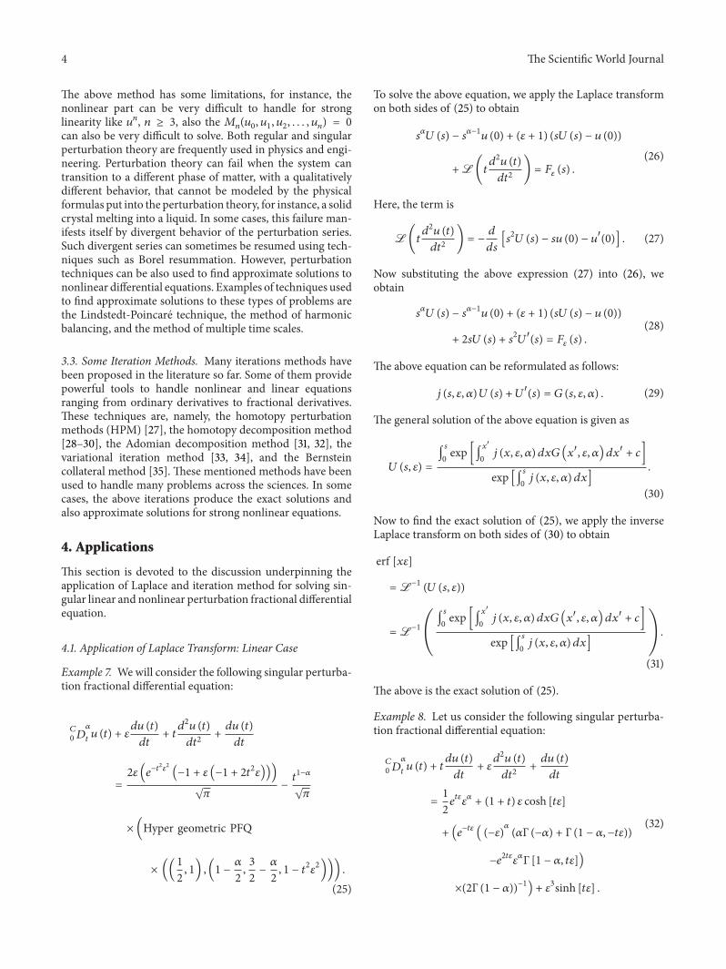


![SINGULAR PERTURBATIONS AND TIME SCALES IN CONTROL …dsnaidu/Naidu_Survey_Zhang-Naidu_et_al_(IJISS)_2014.pdfdynamic equation are discussed on different time scales in [125]. In [456,](https://static.fdocuments.in/doc/165x107/5e6baed7d87b701dbd684af7/singular-perturbations-and-time-scales-in-control-dsnaidunaidusurveyzhang-naiduetalijiss2014pdf.jpg)