Research Article Forecasting Age-Specific Brain Cancer Mortality Rates...

Research ArticleForecasting Age-Specific Brain Cancer Mortality Rates UsingFunctional Data Analysis Models

Keshav P. Pokhrel1 and Chris P. Tsokos2

1Department of Mathematics and Computer Systems, Mercyhurst University, 501 East 38th Street, Erie, PA 16546, USA2Department of Mathematics and Statistics, University of South Florida, 4202 E Fowler Avenue, Tampa, FL 33620, USA

Correspondence should be addressed to Keshav P. Pokhrel; [email protected]

Received 30 July 2014; Revised 2 January 2015; Accepted 20 January 2015

Academic Editor: Peter N. Lee

Copyright © 2015 K. P. Pokhrel and C. P. Tsokos.This is an open access article distributed under theCreativeCommonsAttributionLicense, which permits unrestricted use, distribution, and reproduction in anymedium, provided the originalwork is properly cited.

Incidence and mortality rates are considered as a guideline for planning public health strategies and allocating resources. We applyfunctional data analysis techniques to model age-specific brain cancer mortality trend and forecast entire age-specific functionsusing exponential smoothing state-space models. The age-specific mortality curves are decomposed using principal componentanalysis and fit functional time series model with basis functions. Nonparametric smoothing methods are used to mitigate theexisting randomness in the observed data. We use functional time series model on age-specific brain cancer mortality rates andforecast mortality curves with prediction intervals using exponential smoothing state-space model. We also present a disparity ofbrain cancer mortality rates among the age groups together with the rate of change of mortality rates. The data were obtained fromthe Surveillance, Epidemiology and End Results (SEER) program of the United States. The brain cancer mortality rates, classifiedunder International Classification Disease code ICD-O-3, were extracted from SEER∗Stat software.

1. Introduction

Functional data analysis is about the analysis of informationon curves or functions [1]. Functional data is multivariatedata with an ordering on the dimensions Muller, 2006. Inthe present study we are interested in the distribution offunctions means, covariances, and relationships of functionsto certain responses and other functions. One of the majoradvantages of functional data analysis is a strong possibility ofusing rate of change or derivatives of curves. In this study wecombine methodologies from functional data analysis, non-parametric statistics, and time series forecasting. There hasbeen an intense research in this area during the last decade[2]. In addition, future mortality rates are of great interestsfor strategic planner and the insurance industry. Accurateforecasting can be a strong indicator for allocating budget,planning, and policy making. Here, we develop forecastingmodels for crude mortality rates of malignant primary brainand central nervous system cancer of theUnited States for thestudy period of 1969–2008.

The age-specific mortality rates can play a significant rolefor the allocation of resources for brain tumor control and

evaluations. Primary purpose of this study is to apply func-tional data analysis techniques to model age-specific braincancer mortality time trends and forecast entire age-specificmortality function using state-space-approach [3]. Our aimin the present study is to answer the following questions:

(i) to capture the subtle pattern of variation in mortality,(ii) to find the prediction interval of the forecast,(iii) to find a flexible model so that it could incorporate

the covariates such as screening and treatment effectsinto the analysis.

However, there are some limitation in functional timeseries forecasting model. It only incorporates year of death(calendar period) and fails to consider year of birth (cohort)effects. The calendar period incidence and mortality trendcan reveal the effects of new medical interventions but fail toreflect changes in risk factors such as screening and radiationtherapy.

Currently, most of the forecasting models are based onage-period-cohort methods.Thesemethods are structured toestimate the mortality rates of breast cancer [4], prostate

Hindawi Publishing CorporationAdvances in EpidemiologyVolume 2015, Article ID 721592, 11 pageshttp://dx.doi.org/10.1155/2015/721592

2 Advances in Epidemiology

cancer [5], and cervical cancer [6, 7]. These methods arebasically regression models with mortality or incidence ratesas outcome variables using Poisson error distributionwith loglink function. The most common problem in these modelsis nonidentifiability of parameters, very strong parametricassumptions, and sensitivity of projections and lack ofinclusion of most recent changes in cohort effects. Mostimportantly, a limitation of these studies is that none of themforecast mortality rates with age-related changes.

The linear extrapolation and nonlinear Poisson distribu-tion models are discussed in [8, 9] whereas a Bayesian age-period-cohort model with autoregressive smoothing of eachof age, period, and cohort components is studied such thatthe resulting projections are estimated from current and pasttrends of the data in [4]. Lee and Carter (LC) [10] methodis one of the most influential methods in demographic fore-casting.This is perhaps the most cited paper by demographicresearchers. LC proposed a long term forecasting methodto extrapolate mortality rates and applied it to forecast USmortality rates for the year 2065.

There has been numerous extensions of LCmethod, someof the extensions and modifications of LC method can befound in [11]; Renshaw and Haberman (2003) [12], and theapplications of LCmethod in fertility forecasting can found inLee [13]. The method proposed by Lee and Carter in 1992 hasbecome the leading statistical model of mortality/forecastingin the demographic literature [14], Deaton and Paxson, 2004[15]. It was used as a benchmark for recent Census Bureaupopulation forecasts [16], and twoUS social security technicaladvisory panels recommended its use, or the use of a methodconsistent with it [11].

A comprehensive discussion of the patterns of mortalityrates for then G 7 countries is presented by Tuljapurkar et al.[14] using LC method. The LC model predicted 1-to-4-year higher life expectancy than official projections in theindustrial nations, with larger differences for Japan.

There are numerous uncertainties which affect the mor-tality rates; however a probabilistically sound forecastingmethod, like LC method, is particularly useful to address thelong term funding problems of public pension and insurancefor increasingly ageing population in the industrial world.

2. Functional Data Analysis (FDA) Model

2.1. An Overview. The Lee Carter model for age-specificmortality rates is given by

ln (𝑚𝑥,𝑡) = 𝑎𝑥+ 𝑏𝑥𝑘𝑡+ 𝜖𝑥,𝑡, (1)

where 𝑎𝑥is general age shape of age-specific mortality rates,

𝑏𝑥represents the tendency of mortality at age 𝑥, and 𝑘

𝑡is

the time varying index. Equation (1) is a linear model of anunobserved period-specific intensity index, with parameterdepending on age (LC 1992). LC model uses singular valuedecomposition (SVD) method for exact least square fit; how-ever, a simple linear regression method can also approximatethe parameters. LC incorporates a randomwalk with drift forthe time series formed by 𝑘

𝑡, which is expressed as

𝑘𝑡= 𝑘𝑡−1

+ 𝑐 + 𝑒𝑡, (2)

where 𝑐 is the drift term, 𝑘 is forecast to decline linearly withincrement of 𝑐, and 𝑒

𝑡are permanently incorporated in the

trajectory [11]. The standard error of 𝑐 could be used for thedetailed measure of uncertainty in forecasting 𝑘.

Generalization. The Hyndman-Ullah [3] approach is a gener-alization of Lee and Carter (LC 1992) method.

Our primary goal is to find functional forecasting modelfor mortality rates of brain and central nervous system tumorin the United States. The proposed forecasting model isdeveloped in the realm of functional data [1] for modelinglog mortality rates. To develop the functional data, we invokethe nonparametric smoothing methods to mitigate the exist-ing randomness in the observed information. In addition,the problems related to age groups and issues of outlyingyears are reasonably addressed by using functional princi-pal component [1, 3]. The observed data is smoothed andprincipal component analysis is applied after smoothing theobserved data.

The forecasting methodology by Hyndman-Ullah is ageneralization of Lee and Carter method. This approachuses functional data analysis techniques and treats the age-specific mortality curves as the units of analysis rather thanthe discrete observations [3]. In practice, functional data areusually observed and recorded discretely as 𝑛 pairs (𝑡

𝑗, 𝑦𝑗),

and𝑦𝑗is a snapshot of the function at time 𝑡

𝑗, possibly blurred

by measurement error [1]. Generalized Lee Carter methodmodels themortality rates as a continuous function of age andcaptures the subtle variation between years. In addition thesmoothness of the data reduces the observational error andforecast the entire function with prediction intervals [3].

In the following sectionwediscuss the use ofmore flexible[3] method to model the brain cancer mortality rates whichuses multiple functions to capture the changes in rates.

2.2. FDA Model for Mortality Data. Let 𝑚𝑡(𝑥) denote the

mortality rate for midpoint of age group 𝑥 and year 𝑡, 𝑡 =

1, . . . , 𝑛. We model the log mortality,

𝑦𝑡(𝑡) = log [𝑚

𝑡(𝑥)] , (3)

and assume that there are underlying functions 𝑓𝑡(𝑥) that we

are observing with error [17].Themortality rates as a smoothfunction of age can be expressed as

𝑦𝑡(𝑥𝑖) = 𝑓𝑡(𝑥𝑖) + 𝜎𝑡(𝑥𝑖) 𝜀𝑡,𝑖, (4)

where 𝑥𝑖is the center of age group 𝑖 (𝑖 = 1, . . . , 𝑝), 𝜀

𝑡,𝑖is

an independent and identically distributed standard normalrandom variable, and 𝜎

𝑡(𝑥𝑖) allows the amount of noise to

vary with the age 𝑥. After developing functions of the givenmortality rates, we fit the model

𝑓𝑡(𝑥) = 𝜇 (𝑥) +

𝐾

∑

𝑘=1

𝛽𝑡,𝑘𝜙𝑘(𝑥) + 𝑒

𝑡(𝑥) , (5)

where 𝜇(𝑥) is the mean log mortality rate across years, 𝜙𝑘(𝑥)

is a set of orthogonal basis functions, and 𝑒𝑡(𝑥) is the model

error which is assumed to be serially uncorrelated [17].

Advances in Epidemiology 3

The mean log mortality rates 𝜇(𝑥) are estimated by usingpenalized regression splines (Wood, 2000) [18]. The pairs(𝛽𝑡,𝑘, 𝜙𝑘(𝑥) for 𝑘 = 1, 2, . . . , 𝐾) are estimated by decom-

posing the data into principal components, whereas 𝑒𝑡(𝑥)

is the difference between spline curve and fitted curvefrom the model. We wish to estimate the optimal set of 𝐾orthogonal basis functions. The optimal orthogonal basisfunction 𝜙

𝑘(𝑥) is obtained via principal components (see

Ramsay and Silverman, 2005, pages 151-152). Specifically, fora given 𝐾, we want to find the basis functions {𝜙

𝑘(𝑥)} which

minimizes the mean integrated squared error:

MISE =

1

𝑛

𝑛

∑

𝑡=1

∫ 𝑒2

𝑡(𝑥) 𝑑𝑥. (6)

This is achieved using functional principal components(FPC) decomposition, [19], applied to the curves {𝑓

𝑡(𝑥)}

which provides the least number of basis functions, andexplores the coefficients which are uncorrelated with eachother.

2.3. Forecasting. Equations (4) and (5) together yield

𝑦𝑡(𝑥𝑖) = ln [𝑚

𝑥,𝑡]

= 𝜇 (𝑥) +

𝐾

∑

𝑘=1

𝛽𝑡,𝑘𝜙𝑘(𝑥) + 𝑒

𝑡(𝑥) + 𝜎

𝑡(𝑥𝑖) 𝜀𝑡,𝑖.

(7)

Let 𝛽(𝑛, 𝑘, ℎ) denote the ℎ-step forecast of 𝛽

𝑛+ℎ,𝑘and let

𝑓𝑛,ℎ(𝑥) denote the ℎ-step ahead forecast of 𝑓

𝑛+ℎ(𝑥). Then,

𝑓𝑛,ℎ

(𝑥) = 𝜇 (𝑥) +

𝐾

∑

𝑘=1

𝛽 (𝑛, 𝑘, ℎ)

𝜙𝑘(𝑥) . (8)

To forecast the coefficients from (8) we use state-space modelfor exponential smoothing. The exponential smoothingmethod provides a statistical framework for automatic fore-casting [19]. This forecast then multiplied with estimatedbasis function to obtain the forecast of the entire function. Inaddition, exponential smoothing techniques also provideprediction intervals for the forecast by incorporating varianceof error terms [20]. Forecast from exponential smoothingmethods is estimated recursively where recent observationsare given more weight than historical data. This methodaccommodates additive and multiplicative trend with auto-matic model selection for the given time series [17].

The state-space models provide a convenient and power-ful framework for analyzing sequential data (seeHarvey 1989)[21]. Many mortality data sets require extrapolation, as datahas a time dimension. The state-space model can be used tocalculate smooth feature or signals and associated standarderrors provided the model is of the state-space form.

The sum of the variances of all individual terms is theforecast variance [3]:

Var [𝑦𝑛+ℎ,𝑘

(𝑥)]

= ��2

𝜇(𝑥) +

𝐾

∑

𝑘=1

𝑢𝑛+ℎ,𝑘

𝜙2

𝑘(𝑥) + ] (𝑥) + 𝜎

2

𝑡(𝑥) ,

(9)

where ��2𝜇(𝑥) is the variance obtained using the smoothing

method. The forecast variance is given by

𝑢𝑛+ℎ,𝑘

= Var (𝛽𝑛+ℎ,𝑘|𝛽

1,𝑘,...,𝛽𝑛,𝑘

) , (10)

]𝑘(𝑥): sum of square of residuals, 𝜎2

𝜇(𝑥): variance of the

smooth estimate 𝜇(𝑥), 𝜎2(𝑥) is estimated by assuming bino-mial distribution of 𝑚

𝑡(𝑥), and ](𝑥) is the mean of 𝑒2

𝑡(𝑥) for

each 𝑥.We evaluate the accuracy of the mortality forecast by

computing the mean integrated squared forecasting error(MISFE) defined as

MISFE (ℎ) = 1

𝑛 − 𝑚 + 1

𝑛

∑

𝑡=𝑚

∫ [𝑦𝑡+ℎ

(𝑥) −𝑓𝑡,ℎ(𝑥)]

2

𝑑𝑥,

(11)

where 𝑚 is the minimum number of observations used infitting the model.

3. Data

An estimated 69,720 (10% increment from 2010) new casesof primary nonmalignant and malignant brain and centralnervous system tumors are expected to be diagnosed in theUnited States in 2013 [22].This caused 13,700 (5.5% incrementfrom 2009) deaths because of the primary malignant brainand central nervous system tumors in the United States in2012. It is estimated that 24,620 men and women (13,630men and 10,990 women) will be diagnosed and 13,140 (4.26%increment from 2010) men and women are estimated to bedeceased of brain and other nervous system cancer in 2013.Males and females have a 0.7% and 0.6% lifetime risk of beingdiagnosed with a primary malignant brain/central nervoussystem tumor. These projections are of major public healthinterest. However, their interpretation may be complexbecause of the effect of screening, risk factors, and accessi-bility of effective treatments.

Crude mortality rates per 100,000 persons based onthe 2000 standard US population were extracted using theSEER∗Stat 7.0.5 software of the Surveillance Epidemiologyand End Results program, National Cancer Institute Insti-tutes. We are using 416,480 (229,467 males and 187,013females) malignant Brain cancer patients, where 381,238 arewhites, 24,336 are African Americans, and 4,891 are others(American Indian/AK Native, Asian/Pacific Islander, 1969–2008).

Themortality rateswere at their highest from 1885 to 1995.After 2000we observed that the overall rates are leveling off ordeclining. From 2003–2008, the median age at death for can-cer of the brain and other nervous systemwas 64 years of age.Approximately 4.2% died under age of 20; 3.8% died between20 and 34; 7.1% between 35 and 44; 14.9% between 45 and 54;21.8% between 55 and 64; 22.2% between 65 and 74; 19.6%between 75 and 84; 6.3% died at 85+ years of age. For thefirst part of our study, we use annual crude mortality rates inthe United states from 1969 to 2008 in 5-year age groups (01–04, 05–09,. . .,80–84, 85+).


1970 1980 1990 2000

0

5

10

15

20

25

Male

Years

Mor

talit

y ra

te p

er 1

00,0

00

1924293439444954

59

64

6974

7984

89

Figure 1: Age-specific brain cancer mortality by age group amongtotal males (1969–2008). In the figure 49 represents the age group45–49, 64 represents the age group 60–64, and 89 represent the agegroup above 85.

4. Results

For this study we obtained the data from the Surveillance,Epidemiology and End Results (SEER) program of NationalCancer Institute in the United States [23]. Specifically,mortality data were obtained from the National Center forHealth Statistics (NCHS) available on the SEER∗Statdatabase. Annual age-specific brain cancer mortality data aredesignated by ICD 8 & 9 (1979–1998) code 174 and ICD 10(1999+) codes C70 and C71. The data available is aboutdifferent racial subgroups since 1969 in nineteen year agegroups: 01–04, 05–09, 10–14, 15–19, 20–24, 25–29, 30–34,35–39, 40–44, 45–49, 50–54, 55–59, 60–64, 65–69, 70–74,75–79, 80–84, and 85+.

Figure 1 displays brain cancer mortality rates in US maleby age group for the period of 1969–2007.We observe that themortality rates for ages below 40 years showno obvious trend;for the same period the pattern of mortality rates for agesmore than 40 exhibited significant variation ofmortality ratesfor the elderly. The graph shows the brain cancer mortalityrates among males between 45 and 65 years declined slowlythroughout the study period. The pattern for the elderly(aged 65 and above) population is clearly increasing from1969 to 2000 and started declining after 2000. However,mortality rates for the population subgroups between 45–65show slightly decreasing pattern. The mortality rates for theage groups 80–84 and 85+ are very unstable and difficult tointerpret because of the limited availability of data.

In Figure 2, we present the age-specific mortality rateswith respect to the year of decease for the female subpopu-lation. The trends in mortality rates do not show any visiblepattern for the age groups less than 40 years.The rates for the

1970 1980 1990 2000

0

5

10

15

20

Female

Years

Mor

talit

y ra

te p

er 1

00,0

00

141924293439444954

59

64

69

7479

84

89

Figure 2: Age-specific brain cancer mortality by age group amongtotal females (1969–2008). In the figure 49 represents the age group45–49, 64 represents the age group 60–64, and 89 represent the agegroup above 85.

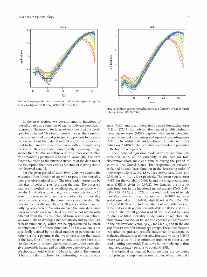
age groups 50–54, 55–59, and 60–64 show decrease in mor-tality during the whole period of study. Overall, the mortalityrate for males is lower than that of female but the age-specificmortality rates show no obvious difference between therates. Figure 3 displays the age-specific mortality rates withrespect to age for the women subpopulation for brain cancermortality rates during the entire period of study, 1969–2008.The graph depicts similar variation of hazard rates as for themale subpopulation. These rates are notably unstable for theyoung (less than 20 years), monotonically increasing formid-dle age population (between 20 and 67), and decreasing withwith strong instability for the elderly (67 and above). In gen-eral, mortality rates are directly proportional to age, and forevery year, highest mortality rates are observed in the agegroups 80–84, 85 and above; this is true for both male andfemale subpopulation.

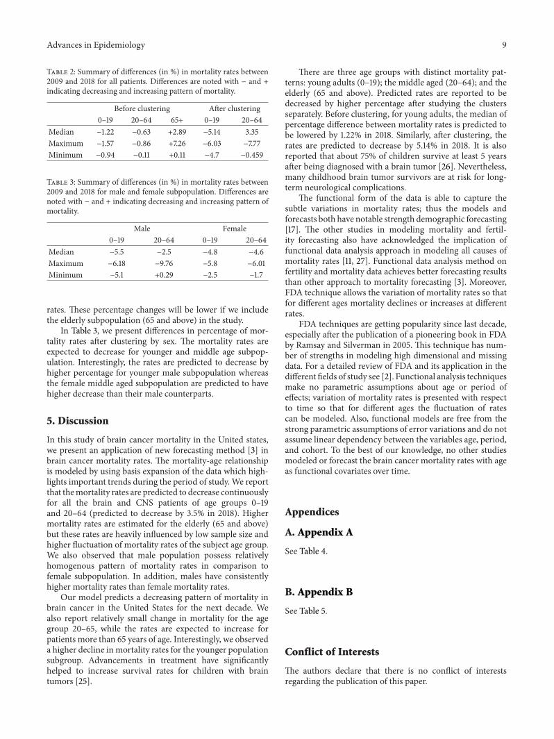
In Figure 4, we present the mortality rates of the malesubpopulation for the entire period of study. The male braincancer mortality rates are higher than female in magnitudebut show similar pattern for different clusters of the popula-tion. Figure 4 clearly indicates three different patterns ofmor-tality rates: first, unstable and decreasing mortality rates forpatients below 20; second, reasonably stable pattern of mor-tality rates for middle aged population subgroups (ages 20–65); and third, significantly increasing and very erratic behav-ior ofmortality rates for the elderly (ages 65 and above).Threedifferent patterns of mortality rates by age are present forthe total population different subgroups of population aswell.However, this behavior of mortality rates is more apparent inmale population.


Female

Age

Log

deat

h ra

te

0 20 40 60 80

−1

0

1

2

3

Figure 3: Age-specific brain cancer mortality with respect to age forfemales subgroup of the population (1969–2008).

In the next section, we develop smooth functions ofmortality rates as a function of age for different populationsubgroups.The smooth (or interpolated) functions are devel-oped for brain and CNS tumor mortality rates; these smoothfunctions are used to find principal components to measurethe variability of the data. Penalized regression splines areused to find smooth functional curve with a monotonicityconstraint. The curves are monotonically increasing for agegreater than 20. The smoothness of the curves is controlledby a smoothing parameter 𝜆 based on Wood [18]. The termfunctional refers to the intrinsic structure of the data underthe assumption that there exists a function of 𝑥 giving rise tothe observed data [1].

For the given period of study 1969–2008, we assume theexistence of the function of age with respect to the mortalityrates plus observational error. The observation errors can bemistakes in collecting or recording the data. The observeddata are smoothed using penalized regression spline withpenalty 𝜆 = 4. We assume that 𝑓

𝑡(𝑥) is monotonic for 𝑥 > 20

years. It is reasonable to assume monotonicity in mortalitydata (the older you are, the more likely you are to die). Thedata are technically smooth after 20 years and there are nooutlying years present. We also analysed the same data usinglinear interpolation as well; final results were not significantlydifferent from the results obtained from regression splines.We would like to develop a mathematically independent setof basis functions 𝜙

𝑘which can be approximated by linear

combination of 𝐾 of these functions. The basis system is notspecifically defined by the fixed number of parameters butrather itself is a parameter that we choose as per the natureof the data. One of the primary criteria to choose basis is totest the behavior of their derivatives; some of the bases thatgive reasonable fitmay end upwith poor derivative estimates.We choose a model with 𝐾 = 6 basis functions. The numberof basis functions is chosen by minimizing the mean square

0 20 40 60 80

0

1

2

3

Male

Age

Log

deat

h ra

teFigure 4: Brain cancer mortality rates as a function of age for malesubpopulation (1969–2008).

error (MSE) and mean integrated squared forecasting error(MISFE) [17, 19]. Six basis functions ended upwithminimummean square error (MSE) together with mean integratedsquared error and mean integrated squared forecasting error(MISFE). No additional basis function contributed in furtherreduction of MISFE.The estimated coefficients are presentedin the bottom of Figure 5.

The functional regression model with six basis functionsexplained 98.8% of the variability of the data for totalobservation (both male and female) during the period ofstudy in the United States. The proportion of variationexplained by each basis function in the decreasing order oftheir magnitude is 92.0%, 4.8%, 0.6%, 0.6%, 0.6%, 0.3%, and0.5% for 𝑘 = 1, . . . , 6, respectively. The mean square error(MSE) for the variability 0.00082 and the integrated squarederror (ISE) is given by 0.07217. For females, the first sixbasis functions in the functional model explain 87.6%, 5.5%,1.8%, 1.1%, 0.8%, and 0.7% of the total variation of femalemortality rates with mean squared error 0.00183 and inte-grated squared error 0.16050, while 88.6%, 4.8%, 1.7%, 1.2%,0.7%, and 0.6% of the total variability of mortality rates areexplained formale populationwithMSE = 0.00153 and ISE =

0.13532. The overall goodness of fit was assessed by usingresiduals of fitted mortality model using image plots. Theplots showed no lack of fit. We also checked autocorrelationin the observational error, 𝜖

𝑡(𝑥𝑖), for each 𝑥

𝑖and in the one

step forecast error for various age groups.The autocorrelationwas either insignificant or sufficiently small. In addition, weevaluated the accuracy of mortality forecasts by usingMISFEwhere we set 𝑚 = 10 as minimum number of observationsused in fitting the model. That is, we fit the model up to time𝑡 and predict next 𝑛 periods to obtain MISFE.

The optimal orthogonal basis functions are computedfrom principal component decomposition. We want to find a


0.0

0.5

1.0

1.5

2.0

2.5

Total US

0 20 40 60 80Age

0 20 40 60 80 0 20 40 60 80 0 20 40 60 80 0 20 40 60 80

0 20 40 60 80Age

0 20 40 60 80Age

0.0

0.05

0.10

0.15

0.0

0.1

0.2

0.0

0.1

0.2

0.0

0.1

0.2

0.0

0.1

0.2

0.3

−0.5

−0.2

−0.1

−0.3

−0.2

−0.1

−0.1

−0.1

−0.3

−0.2

−0.1

𝜙1

𝜙2

𝜙3

𝜙4

𝜙5

𝜙6

𝜇(x)

(a)

Year1970 1990 2010

Year1970 1990 2010

Year1970 1990 2010

1970 1990 20101970 1990 20101970 1990 2010

0

2

4

0.0

0.5

0.0

0.2

0.4

0.0

0.1

0.2

0.3

0.0

0.2

−0.2

−0.1

0.0

0.1

0.2

−0.4

−0.2

−0.4

−0.2

−0.3

−0.2

−0.1

−1.5

−0.5

−1.0

−4

−2

𝛽1

𝛽2

𝛽3

𝛽4

𝛽5

𝛽6

(b)

Figure 5:The functional model for brain cancer mortality in the USA. Top line: the mean function and first six basis functions. Bottom line:the coefficients associated with each of the basis functions.


set of exactly𝐾 orthogonal functions𝜙𝑘so that the expansion

of each curve in terms of these basis functions approximatesthe curve as closely as possible (see Ramsay and Silverman,2005, pages 151-152). Figure 5 explores the first six basisfunctions together with the corresponding coefficients. Thebasis functions and the time series coefficients model theoverall variability of the mortality rates. The first basisfunction (𝜙

1)models the higher age groups (around 80 years),

as the score is the largest in negative direction; second basisfunction (𝜙

2) models the middle age (20–65); the third and

fourth (𝜙3and 𝜙

4) basis functions represent the infants and

people under 20 years of age respectfully. The fifth and sixth(𝜙5and 𝜙

6) are relatively complex to explain and we are

not attempting to explain these functions because of theirunpredictable variability.

The plots of time series coefficients, Figure 5, depict acontinuously increasing pattern before 1990, while the ratesshow a declining pattern during the decade of 1990–2000.The first time series coefficients represent decreasing trendbut since the basis function has negative sign, the older ages(around 80 years) have been increasing during the studyperiod and it can also be observed from Figure 3.The secondtime series is first increasing till 1990 and then decreasingwhich corresponds to the age group 20–40 years. Morespecifically, the mortality rates are increasing for the agegroups more than 65, slightly decreasing for the populationwith the age between 40 and 65, and the rates are leveled offfor younger population. The variability of mortality rates forthe patients more than 80 years is remarkably high, which isnumerically important and less explained by the basis func-tions. The erratic death rates for the elderly may be becauseof the measurement error than due to behavior of the rates.Similar study by Coale and Kisker [24] showed that themortality data are highly susceptible and fraught with varioustypes of measurement problems. It is more reasonable tohave detail and separate study of patients above 80 years; weexcluded themortality rates for the age groups 80–84 and 85+in the later part of our study.

The forecast of the brain cancer mortality rates is calcu-lated by multiplying the time series coefficients with the basisfunctions. Figure 6 shows 10-year forecast of mortality ratesfor male and female together during the period of study. Weobserve that the brain and CNS cancer mortality rates areexpected to increase with respect to age. One-year and ten-year forecast show a declining pattern of mortality rates forbrain and CNS tumor patients of all the age groups. A declin-ing pattern of mortality rates is observed for the ages lessthan 60. However, the declining pattern of mortality rates isinverted for the elderly.

The difference between the mortality rates is remarkablyhigher in the age groups more than 75 years. Averagedifference of mortality rates in the age groups 75–79, 80–84,85–89, and 89+ is 0.05 per 100,000 per year. We observe thatthe average mortality rates of a person of 62 years of age isalmost 10 times higher than that of a person of 32 years of age.Long term forecast shows that the rates are predicted todecline relatively slowly in the next decade. The mortalityrates for the total US population are expected to decrease by1.58% for the age group of 0–4 years, and at the same time

0 20 40 60 80

−1

0

1

2

3

Total US

Age

Log

deat

h ra

te

2009

2018

Figure 6: Forecast of age-specificmortality of total brain and centralnervous system cancer patients in the United States for 2009 and2018, with 80% confidence intervals.

rates are expected to increase by 5.5% for the age group of 80–84. Specifically, the mortality rates are predicted to increasefor all the persons above 65 years of age. For total US popu-lation with age less than or equal to 65 the rates are predictedto decrease linearly at the rate of 0.0145 per 100,0000 peryear (𝑃 value < 0.05). We also observed that 20th percentileof difference in mortality rates between 2009 and 2018 is0.501 per 100,000 pear year; 50th percentile is 0.796; and99 percentile of the difference between mortality rates is 1.57per 100,000 per year.

In Figure 7, we present one-year and ten-year predictionintervals formale and female populations.Themortality ratesare expected to increase, (comparing with 2009) for boththe gender by 0.17 (0.37%) persons per 100,000 by 2018.For the same period the mortality rates for males and femalesseparately are expected to increase by 0.33 (0.78%) and 0.11(0.19%) persons per 100,000 by 2018. This may be becauseof erratically higher mortality rates of elderly population.However, age-specific forecast for 2009 and 2018 showsslower rate of decline in female mortality rates in comparisonto the male population. The average increment in mortalityrates is 0.33 persons per 100,000 and 0.84 persons per 100000for males and females aged below 65 years, respectively. Wealso observed that the mortality rate for the age groups morethan 65 is increasing in higher rate than other age groups.Theaverage rate of increase in mortality rates for the elderly is1.23 (5%) and 0.44 (0.38%) persons per 100000 for males andfemales, respectively (see Table 1). The mortality rates for theelderly population are subject to error because of availabilityof information and erratic behavior in themortality rates. Leeand Carter (1991) [10] also mentioned the unreliability ofage groups 85+. In contrast, after clustering the ages intothree groups, 0–19 (young adults), 20–64 (middle age), and65 and above (elderly), we observe that the mortality rates foryounger population are estimated to decrease with the high-est declining rate followed by the middle aged population.

In Table 1, we present one-year and ten-year forecast ofthe mortality rates. The average decrease (from 2009 to 2018)in mortality rates for male and female subpopulation is 1.6and 1.41 persons per 100,000. The variability of the mortalityrates for different age groups is clearly noticeable. Despite the


Female4

Male

0 20 40 60 80

−1

0

1

2

3

Age

Log

deat

h ra

te

2009

2018

0 20 40 60 80

−1

0

1

2

3

Age

Log

deat

h ra

te

2009

2018

Figure 7: Forecast of age-specific mortality of brain and central nervous system cancer in the United States for 2009 and 2018 for male andfemale subpopulation with 80% confidence intervals.

Table 1: Forecast and 80% prediction intervals of mortality rates of total US patients of brain and CNS tumors for 2009 and 2018.

AgeTotal Male Female

2009 2018 2009 2018 2009 2018Mean 80% PI Mean 80% PI Mean 80% PI Mean 80% PI Mean 80% PI Mean 80% PI

2 0.62 0.55 0.70 0.61 0.53 0.70 0.66 0.56 0.79 0.65 0.54 0.78 0.57 0.49 0.66 0.56 0.47 0.677 0.88 0.80 0.97 0.87 0.78 0.97 0.87 0.76 0.99 0.85 0.74 0.98 0.88 0.78 1.00 0.88 0.77 1.0012 0.63 0.56 0.71 0.62 0.55 0.71 0.63 0.55 0.74 0.62 0.53 0.74 0.62 0.53 0.71 0.61 0.52 0.7117 0.48 0.44 0.53 0.48 0.42 0.54 0.53 0.46 0.61 0.53 0.45 0.62 0.42 0.37 0.49 0.42 0.35 0.4922 0.53 0.48 0.58 0.52 0.47 0.59 0.62 0.53 0.72 0.60 0.51 0.71 0.42 0.34 0.52 0.42 0.33 0.5327 0.73 0.66 0.80 0.72 0.64 0.81 0.86 0.75 0.99 0.86 0.73 1.00 0.53 0.45 0.63 0.54 0.43 0.6632 1.10 1.01 1.20 1.09 0.97 1.22 1.33 1.20 1.47 1.32 1.16 1.50 0.84 0.73 0.98 0.84 0.70 1.0037 1.63 1.51 1.76 1.62 1.46 1.79 2.00 1.83 2.19 1.99 1.78 2.22 1.24 1.11 1.39 1.23 1.07 1.4242 2.49 2.33 2.66 2.47 2.27 2.70 3.10 2.84 3.39 3.08 2.78 3.42 1.90 1.71 2.10 1.88 1.66 2.1247 3.70 3.45 3.97 3.67 3.36 4.01 4.58 4.20 4.99 4.54 4.10 5.03 2.87 2.61 3.15 2.85 2.54 3.1852 5.48 5.17 5.81 5.45 5.02 5.91 6.73 6.25 7.25 6.69 6.10 7.33 4.29 3.94 4.66 4.26 3.82 4.7557 8.00 7.62 8.41 7.95 7.40 8.54 9.73 9.13 10.38 9.69 8.93 10.50 6.29 5.84 6.78 6.26 5.67 6.9162 10.84 10.30 11.41 10.80 10.05 11.60 13.25 12.50 14.06 13.27 12.33 14.27 8.56 7.88 9.30 8.55 7.68 9.5367 13.88 13.20 14.61 13.91 12.91 14.99 16.83 15.71 18.02 17.01 15.59 18.56 11.13 10.32 12.00 11.17 10.10 12.3772 17.14 16.05 18.31 17.40 15.70 19.28 20.64 19.15 22.26 21.21 19.11 23.54 14.18 12.93 15.54 14.37 12.62 16.3677 19.22 17.62 20.96 19.77 17.10 22.86 23.81 21.65 26.19 24.87 21.76 28.42 15.59 13.90 17.48 15.98 13.31 19.1982 19.94 17.30 22.98 21.05 16.60 26.69 24.69 20.94 29.11 26.64 21.17 33.51 16.66 14.10 19.69 17.35 13.12 22.9587 17.44 14.63 20.78 18.70 13.89 25.19 23.30 19.00 28.57 25.72 19.24 34.38 14.52 11.82 17.82 15.38 10.89 21.73

fact that brain and CNS cancer is one of the most vulnerablecancer for the younger population, the mortality rates aredeclining faster thanmiddle aged and elderly population. In aseparate study of mortality rates for the age groups 0–19 and20–64 we report smaller MSE as well ISE in comparison tothemodels with age groups together (see Appendices A and Bfor forecast of the mortality rates for age groups 0–19 and 20–65).

In Tables 2 and 3, we present predicted change inpercentage of mortality rates between 2009 and 2018. Table 2shows the mortality rates are increasing for the elderly agegroup whereas the case is inverted for other two age groups.In addition, we can expect that 50% ormore younger patientswill see 5.14% reduction ofmortality rates in the younger sub-population in 2018 whereas 50% of the middle aged patient(20–65) are predicted to have 3.35% reduction in mortality


Table 2: Summary of differences (in %) in mortality rates between2009 and 2018 for all patients. Differences are noted with − and +indicating decreasing and increasing pattern of mortality.

Before clustering After clustering0–19 20–64 65+ 0–19 20–64

Median −1.22 −0.63 +2.89 −5.14 3.35Maximum −1.57 −0.86 +7.26 −6.03 −7.77Minimum −0.94 −0.11 +0.11 −4.7 −0.459

Table 3: Summary of differences (in %) in mortality rates between2009 and 2018 for male and female subpopulation. Differences arenoted with − and + indicating decreasing and increasing pattern ofmortality.

Male Female0–19 20–64 0–19 20–64

Median −5.5 −2.5 −4.8 −4.6Maximum −6.18 −9.76 −5.8 −6.01Minimum −5.1 +0.29 −2.5 −1.7

rates. These percentage changes will be lower if we includethe elderly subpopulation (65 and above) in the study.

In Table 3, we present differences in percentage of mor-tality rates after clustering by sex. The mortality rates areexpected to decrease for younger and middle age subpop-ulation. Interestingly, the rates are predicted to decrease byhigher percentage for younger male subpopulation whereasthe female middle aged subpopulation are predicted to havehigher decrease than their male counterparts.

5. Discussion

In this study of brain cancer mortality in the United states,we present an application of new forecasting method [3] inbrain cancer mortality rates. The mortality-age relationshipis modeled by using basis expansion of the data which high-lights important trends during the period of study. We reportthat themortality rates are predicted to decrease continuouslyfor all the brain and CNS patients of age groups 0–19and 20–64 (predicted to decrease by 3.5% in 2018). Highermortality rates are estimated for the elderly (65 and above)but these rates are heavily influenced by low sample size andhigher fluctuation of mortality rates of the subject age group.We also observed that male population possess relativelyhomogenous pattern of mortality rates in comparison tofemale subpopulation. In addition, males have consistentlyhigher mortality rates than female mortality rates.

Our model predicts a decreasing pattern of mortality inbrain cancer in the United States for the next decade. Wealso report relatively small change in mortality for the agegroup 20–65, while the rates are expected to increase forpatients more than 65 years of age. Interestingly, we observeda higher decline inmortality rates for the younger populationsubgroup. Advancements in treatment have significantlyhelped to increase survival rates for children with braintumors [25].

There are three age groups with distinct mortality pat-terns: young adults (0–19); the middle aged (20–64); and theelderly (65 and above). Predicted rates are reported to bedecreased by higher percentage after studying the clustersseparately. Before clustering, for young adults, the median ofpercentage difference between mortality rates is predicted tobe lowered by 1.22% in 2018. Similarly, after clustering, therates are predicted to decrease by 5.14% in 2018. It is alsoreported that about 75% of children survive at least 5 yearsafter being diagnosed with a brain tumor [26]. Nevertheless,many childhood brain tumor survivors are at risk for long-term neurological complications.

The functional form of the data is able to capture thesubtle variations in mortality rates; thus the models andforecasts both have notable strength demographic forecasting[17]. The other studies in modeling mortality and fertil-ity forecasting also have acknowledged the implication offunctional data analysis approach in modeling all causes ofmortality rates [11, 27]. Functional data analysis method onfertility and mortality data achieves better forecasting resultsthan other approach to mortality forecasting [3]. Moreover,FDA technique allows the variation of mortality rates so thatfor different ages mortality declines or increases at differentrates.

FDA techniques are getting popularity since last decade,especially after the publication of a pioneering book in FDAby Ramsay and Silverman in 2005. This technique has num-ber of strengths in modeling high dimensional and missingdata. For a detailed review of FDA and its application in thedifferent fields of study see [2]. Functional analysis techniquesmake no parametric assumptions about age or period ofeffects; variation of mortality rates is presented with respectto time so that for different ages the fluctuation of ratescan be modeled. Also, functional models are free from thestrong parametric assumptions of error variations and do notassume linear dependency between the variables age, period,and cohort. To the best of our knowledge, no other studiesmodeled or forecast the brain cancer mortality rates with ageas functional covariates over time.

Appendices

A. Appendix A

See Table 4.

B. Appendix B

See Table 5.

Conflict of Interests

The authors declare that there is no conflict of interestsregarding the publication of this paper.


Table 4: Age- and gender-specific prediction of brain cancer mortality rates of young adults for the years 2009 and 2018. In the first table,prediction is made for all the patients under study. In the second table, perdition of mortality rates is made separately for young adults (0–19years). Prediction of mortality rates show higher decreasing rate if analysis is done after clustering the data by age groups.

(a)



2 0.62 0.55 0.70 0.61 0.53 0.70 0.66 0.56 0.79 0.65 0.54 0.78 0.57 0.49 0.66 0.56 0.47 0.677 0.88 0.80 0.97 0.87 0.78 0.97 0.87 0.76 0.99 0.85 0.74 0.98 0.88 0.78 1.00 0.88 0.77 1.0012 0.63 0.56 0.71 0.62 0.55 0.71 0.63 0.55 0.74 0.62 0.53 0.74 0.62 0.53 0.71 0.61 0.52 0.7117 0.48 0.44 0.53 0.48 0.42 0.54 0.53 0.46 0.61 0.53 0.45 0.62 0.42 0.37 0.49 0.42 0.35 0.49

(b)



2 0.63 0.56 0.71 0.59 0.52 0.67 0.66 0.56 0.79 0.62 0.52 0.74 0.59 0.51 0.69 0.56 0.48 0.657 0.84 0.76 0.92 0.80 0.73 0.89 0.81 0.71 0.93 0.77 0.67 0.88 0.86 0.76 0.97 0.84 0.74 0.9412 0.61 0.55 0.68 0.58 0.52 0.65 0.64 0.55 0.74 0.60 0.52 0.70 0.56 0.49 0.65 0.54 0.47 0.6217 0.50 0.45 0.55 0.47 0.42 0.52 0.57 0.49 0.66 0.54 0.46 0.62 0.42 0.36 0.48 0.39 0.34 0.46

Table 5: Age- and gender-specific prediction of brain cancer mortality rates of young adults for the years 2009 and 2018. In the first table,prediction is made for all the patients under study. In the second table, perdition of mortality rates is made separately for middle age (20–64years) subpopulation. Prediction of mortality rates show higher decreasing rate if analysis is done after clustering the data by age groups.

(a)



22 0.53 0.48 0.58 0.52 0.47 0.59 0.62 0.53 0.72 0.60 0.51 0.71 0.42 0.34 0.52 0.42 0.33 0.5327 0.73 0.66 0.80 0.72 0.64 0.81 0.86 0.75 0.99 0.86 0.73 1.00 0.53 0.45 0.63 0.54 0.43 0.6632 1.10 1.01 1.20 1.09 0.97 1.22 1.33 1.20 1.47 1.32 1.16 1.50 0.84 0.73 0.98 0.84 0.70 1.0037 1.63 1.51 1.76 1.62 1.46 1.79 2.00 1.83 2.19 1.99 1.78 2.22 1.24 1.11 1.39 1.23 1.07 1.4242 2.49 2.33 2.66 2.47 2.27 2.70 3.10 2.84 3.39 3.08 2.78 3.42 1.90 1.71 2.10 1.88 1.66 2.1247 3.70 3.45 3.97 3.67 3.36 4.01 4.58 4.20 4.99 4.54 4.10 5.03 2.87 2.61 3.15 2.85 2.54 3.1852 5.48 5.17 5.81 5.45 5.02 5.91 6.73 6.25 7.25 6.69 6.10 7.33 4.29 3.94 4.66 4.26 3.82 4.7557 8.00 7.62 8.41 7.95 7.40 8.54 9.73 9.13 10.38 9.69 8.93 10.50 6.29 5.84 6.78 6.26 5.67 6.9162 10.84 10.30 11.41 10.80 10.05 11.60 13.25 12.50 14.06 13.27 12.33 14.27 8.56 7.88 9.30 8.55 7.68 9.53

(b)



22 0.50 0.45 0.55 0.46 0.40 0.52 0.57 0.50 0.67 0.52 0.44 0.61 0.39 0.32 0.48 0.36 0.29 0.4527 0.71 0.65 0.78 0.68 0.62 0.76 0.83 0.73 0.95 0.82 0.71 0.95 0.55 0.47 0.66 0.52 0.44 0.6232 1.08 0.99 1.18 1.04 0.94 1.15 1.41 1.28 1.56 1.32 1.18 1.47 0.82 0.71 0.94 0.77 0.66 0.9037 1.57 1.46 1.69 1.52 1.39 1.66 2.02 1.85 2.20 1.90 1.72 2.10 1.21 1.08 1.35 1.15 1.02 1.3042 2.41 2.25 2.58 2.33 2.15 2.52 3.03 2.78 3.31 2.99 2.72 3.29 1.81 1.62 2.02 1.73 1.53 1.9547 3.56 3.32 3.82 3.44 3.17 3.73 4.50 4.14 4.90 4.38 3.99 4.81 2.77 2.51 3.06 2.65 2.37 2.9552 5.36 5.06 5.67 5.19 4.84 5.57 6.59 6.12 7.09 6.47 5.95 7.03 4.23 3.88 4.60 4.05 3.68 4.4557 7.89 7.50 8.30 7.72 7.27 8.21 9.79 9.17 10.46 9.50 8.84 10.21 6.33 5.86 6.84 6.13 5.63 6.6862 11.00 10.35 11.69 10.95 10.25 11.70 13.45 12.65 14.30 13.49 12.64 14.40 8.87 8.13 9.68 8.71 7.95 9.55


References

[1] J. O. Ramsay and B. W. Silverman, Functional Data Analysis,Springer, New York, NY, USA, 2005.

[2] S. Ullah and C. F. Finch, “Applications of functional data anal-ysis: a systematic review,” BMC Medical Research Methodology,vol. 13, article 43, pp. 539–572, 2013.

[3] R. J. Hyndman andM. S. Ullah, “Robust forecasting ofmortalityand fertility rates: a functional data approach,” ComputationalStatistics & Data Analysis, vol. 51, no. 10, pp. 4942–4956, 2007.

[4] S. A. Bashir and J. Esteve, “Projecting cancer incidence andmortality using Bayesian age-period-cohort models,” Journal ofEpidemiology and Biostatistics, vol. 6, no. 3, pp. 287–296, 2001.

[5] E. A. Eisen, J. Bardin, R. Gore, S. R. Woskie, M. F. Hallock, andR. R. Monson, “Exposure-response models based on extendedfollow-up of a cohort mortality study in the automobile indus-try,” Scandinavian Journal of Work, Environment and Health,vol. 27, no. 4, pp. 240–249, 2001.

[6] L. Hristova, I. Dimova, and M. Iltcheva, “Projected cancerincidence rates in Bulgaria, 1968–2017,” International Journal ofEpidemiology, vol. 26, no. 3, pp. 469–475, 1997.

[7] E. Negri, C. la Vecchia, F. Levi, A. Randriamiharisoa, A. Decarli,and P. Boyle, “The application of age, period and cohort modelsto predict Swiss cancer mortality,” Journal of Cancer Researchand Clinical Oncology, vol. 116, no. 2, pp. 207–214, 1990.

[8] T. Dyba, T. Hakulinen, and L. Paivarinta, “A simple non-linearmodel in incidence prediction,” Statistics inMedicine, vol. 16, no.20, pp. 2297–2309, 1997.

[9] T. Dyba and T. Hakulinen, “Comparision of differentapproaches to incidence prediction based on simple inter-polation techniques,” Statistics in Medicine, vol. 19, no. 13, pp.1741–1752, 2000.

[10] R. D. Lee and L. Carter, “Modeling and forecasting U. S.mortality,” Journal of the American Statisticial Association, vol.87, no. 419, pp. 659–671, 1992.

[11] R. Lee and T. Miller, “Evaluating the performance of Lee-Carter mortality forecasts,” pp. 1–17, 2000, http://www.demog.berkeley.edu.

[12] A. E. Renshaw and S. Haberman, “On the forecasting of mortal-ity reduction factors,” Insurance: Mathematics and Economics,vol. 32, no. 3, pp. 379–401, 2003.

[13] R. D. Lee, “Modeling and forecasting the time series of US fer-tility: age distribution, range, and ultimate level,” InternationalJournal of Forecasting, vol. 9, no. 2, pp. 187–202, 1993.

[14] S. Tuljapurkar, N. Li, and C. Boe, “A universal pattern ofmortality decline in the G7 countries,” Nature, vol. 405, no.6788, pp. 789–792, 2000.

[15] A. Deaton and C. Paxson, “Mortality, income, and incomeinequality over time in the Britain and the United States,” Tech.Rep. 8534, National Bureau of Economic Research, Cambridge,Mass, USA, 2004.

[16] F. Hollmann, J. Tammany, and J. Kallan, “Methodology andassumptions for the population projections of the UnitedStates: 1999 to 2100. Population division, bureau of the census,population division,” International Journal of Forecasting, vol.38, 2000.

[17] B. Erbas, R. J. Hyndman, and D. M. Gertig, “Forecasting age-specific breast cancer mortality using functional data models,”Statistics in Medicine, vol. 26, no. 2, pp. 458–470, 2007.

[18] S. N. Wood, “Modelling and smoothing parameter estimationwith multiple quadratic penalties,” Journal of the Royal Statisti-cal Society Series B, vol. 62, no. 2, pp. 413–428, 2000.

[19] F. Yasmeen, R. J. Hyndman, and B. Erbas, “Forecasting age-related changes in breast cancer mortality among white andblack US women: a functional data approach,” Cancer Epidemi-ology, vol. 34, no. 5, pp. 542–549, 2010.

[20] R. J. Hyndman and Y. Khandakar, “Automatic time seriesforecasting: the forecast package for R,” Journal of StatisticalSoftware, vol. 27, no. 3, pp. 1–22, 2008.

[21] A. C. Harvey, Forecasting, Structural Time Series Models and theKalman Filter, Cambridge University Press, Cambridge, UK,1992.

[22] CBTRUS, American Cancer Society, Brain Cancer Facts Sheets:Brain and Other Nervous System. Atlanta, GA, 2010. CentralBrain Tumor Registry of the United States [CBTRUS]: CBTRUSStatistical Report. Primary Brain and Central Nervous SystemTumors Diagnosed in the United States in 2004-2006, CBTRUS,2010.

[23] SEER, Surveillance, Epidemiology, and End Results (SEER)Program. SEER Stat Database: Mortality—All COD, Aggregatedwith State, Total U.S. (1969–2007) <Katrina/Rita PopulationAdjustment>, National Cancer Institute, DCCPS, SurveillanceResearch Program, Cancer Statistics Branch, June 2010. Under-lying Mortality Data Provided by NCHS, National Insitute ofHealth, 2010.

[24] A. J. Coale and E. E. Kisker, “Defects in data on old agemortality in the United States: new procedures for calculatingapproximately accuratemortality schedules and life tables at thehighest ages,”Asian& Pacific Population Forum, vol. 4, no. 1, pp.1–31, 1990.

[25] L. Legler, J.M.Ries,M. Smith et al., “Brain and other central ner-vous system cancers: recent trends in incedence and mortality,”Journal of National Cancer Institute, vol. 91, no. 2, pp. 1382–1389,1999.

[26] J. P. Neglia, L. L. Robison, M. Stovall et al., “New primary neo-plasms of the central nervous system in survivors of childhoodcancer: a report from the Childhood Cancer Survivor Study,”Journal of the National Cancer Institute, vol. 98, no. 21, pp. 1528–1537, 2006.

[27] S. Horiuchi and J. Wilmoth, “The aging of mortality decline,” inProceedings of the AnnualMeetings of the Population Associationof America, San Francisco, Calif, USA, August 2005.

Submit your manuscripts athttp://www.hindawi.com

Stem CellsInternational

Hindawi Publishing Corporationhttp://www.hindawi.com Volume 2014


MEDIATORSINFLAMMATION

of


Behavioural Neurology

EndocrinologyInternational Journal of



Disease Markers


BioMed Research International

OncologyJournal of



Oxidative Medicine and Cellular Longevity


PPAR Research

The Scientific World JournalHindawi Publishing Corporation http://www.hindawi.com Volume 2014

Immunology ResearchHindawi Publishing Corporationhttp://www.hindawi.com Volume 2014

Journal of

ObesityJournal of



Computational and Mathematical Methods in Medicine

OphthalmologyJournal of


Diabetes ResearchJournal of



Research and TreatmentAIDS


Gastroenterology Research and Practice


Parkinson’s Disease

Evidence-Based Complementary and Alternative Medicine

Volume 2014Hindawi Publishing Corporationhttp://www.hindawi.com

Research Article Forecasting Age-Specific Brain Cancer Mortality Rates...

Documents

Transcript of Research Article Forecasting Age-Specific Brain Cancer Mortality Rates...