
Research Article Efficiency of Hysteresis Rods in Small ...
18
Hindawi Publishing Corporation e Scientific World Journal Volume 2013, Article ID 459573, 17 pages http://dx.doi.org/10.1155/2013/459573 Research Article Efficiency of Hysteresis Rods in Small Spacecraft Attitude Stabilization Assal Farrahi and Ángel Sanz-Andrés Instituto Universitario de Microgravedad “Ignacio Da Riva” (IDR), ETSI Aeronauticos, Universidad Polit´ ecnica de Madrid, Plaza del Cardenal Cisneros 3, 28040 Madrid, Spain Correspondence should be addressed to Assal Farrahi; [email protected] Received 12 October 2013; Accepted 1 December 2013 Academic Editors: D. Missirlis and F. Topputo Copyright © 2013 A. Farrahi and ´ A. Sanz-Andr´ es. is is an open access article distributed under the Creative Commons Attribution License, which permits unrestricted use, distribution, and reproduction in any medium, provided the original work is properly cited. A semiempirical method for predicting the damping efficiency of hysteresis rods on-board small satellites is presented. It is based on the evaluation of dissipating energy variation of different ferromagnetic materials for two different rod shapes: thin film and circular cross-section rods, as a function of their elongation. Based on this formulation, an optimum design considering the size of hysteresis rods, their cross section shape, and layout has been proposed. Finally, the formulation developed was applied to the case of four existing small satellites, whose corresponding in-flight data are published. A good agreement between the estimated rotational speed decay time and the in-flight data has been observed. 1. Introduction Although the technology of Passive Magnetic Attitude Sta- bilization Systems (PMASS) started to be developed in 1961 [1, 2] and has been applied to several small size satellites [3], there are still some issues to be solved regarding this system, such as the sizing of its system parameters and predicting the in-orbit performance without going through long experimental procedures. ese problems are rooted in the difficulties that exist in determining the magnetic characteristics of the ferromagnetic bodies (hysteresis rods) that are applied as damping devices on-board the satellites, as the variation of these characteristics is a complex function of different variables that might not be very well known. One of the earliest investigations in this field was carried out by Fischell [4]. According to this work, the magnetic properties of the ferromagnetic bodies, apart from the properties of the material, were seen to be very sensitive to the body length-to-thickness ratio (elongation). rough experimental results of Fischell [4] it was seen that the rod with higher value of elongation presented a larger damping capacity. Also the cross-section shape and size of the rods are the other known factors that strongly affect the magnetic properties of the hysteresis rods, as the damping capacity of a hysteresis rod is directly proportional to its volume. ere- fore, for rods with the same shape and elongation, the bigger the rod is, the larger its corresponding damping capacity will be. Evidently, the length of the rod cannot exceed the lateral dimensions of the satellite. us, for increasing the volume of the body its other dimensions should be increased. However, increasing the thickness leads to a reduction of elongation and consequently damping capacity of the rod. Considering these effects together, it is expected that an optimum value for the thickness of the hysteresis rods exists, for which the corresponding efficiency of the rod is a maximum. is problem has been recently studied to some extent in [5], in which the energy dissipated by in Film Rods (TFR) made up of different materials has been studied and the corresponding optimum thickness has been evaluated for different materials. By TFRs we are referring to rods with rectangular cross-sections and a thickness less than 1 mm. In addition to the material, shape, elongation, and vol- ume, experimental data show that the heat treatment and manufacturing process are also parameters that influence the magnetic properties of ferromagnetic bodies; however, the exact influence cannot be predicted theoretically yet [6, 7]. Some experimental results concerning the variation
Transcript of Research Article Efficiency of Hysteresis Rods in Small ...

Hindawi Publishing CorporationThe Scientific World JournalVolume 2013 Article ID 459573 17 pageshttpdxdoiorg1011552013459573
Research ArticleEfficiency of Hysteresis Rods in Small SpacecraftAttitude Stabilization
Assal Farrahi and Aacutengel Sanz-Andreacutes
Instituto Universitario de Microgravedad ldquoIgnacio Da Rivardquo (IDR) ETSI Aeronauticos Universidad Politecnica de MadridPlaza del Cardenal Cisneros 3 28040 Madrid Spain
Correspondence should be addressed to Assal Farrahi assalfarrahiupmes
Received 12 October 2013 Accepted 1 December 2013
Academic Editors D Missirlis and F Topputo
Copyright copy 2013 A Farrahi and A Sanz-Andres This is an open access article distributed under the Creative CommonsAttribution License which permits unrestricted use distribution and reproduction in any medium provided the original work isproperly cited
A semiempirical method for predicting the damping efficiency of hysteresis rods on-board small satellites is presented It is basedon the evaluation of dissipating energy variation of different ferromagnetic materials for two different rod shapes thin film andcircular cross-section rods as a function of their elongation Based on this formulation an optimum design considering the sizeof hysteresis rods their cross section shape and layout has been proposed Finally the formulation developed was applied to thecase of four existing small satellites whose corresponding in-flight data are published A good agreement between the estimatedrotational speed decay time and the in-flight data has been observed
1 Introduction
Although the technology of Passive Magnetic Attitude Sta-bilization Systems (PMASS) started to be developed in 1961[1 2] and has been applied to several small size satellites[3] there are still some issues to be solved regarding thissystem such as the sizing of its system parameters andpredicting the in-orbit performance without going throughlong experimental procedures These problems are rootedin the difficulties that exist in determining the magneticcharacteristics of the ferromagnetic bodies (hysteresis rods)that are applied as damping devices on-board the satellites asthe variation of these characteristics is a complex function ofdifferent variables that might not be very well known
One of the earliest investigations in this field was carriedout by Fischell [4] According to this work the magneticproperties of the ferromagnetic bodies apart from theproperties of the material were seen to be very sensitiveto the body length-to-thickness ratio (elongation) Throughexperimental results of Fischell [4] it was seen that the rodwith higher value of elongation presented a larger dampingcapacity
Also the cross-section shape and size of the rods arethe other known factors that strongly affect the magnetic
properties of the hysteresis rods as the damping capacity ofa hysteresis rod is directly proportional to its volume There-fore for rods with the same shape and elongation the biggerthe rod is the larger its corresponding damping capacity willbe Evidently the length of the rod cannot exceed the lateraldimensions of the satelliteThus for increasing the volume ofthe body its other dimensions should be increased Howeverincreasing the thickness leads to a reduction of elongationand consequently damping capacity of the rod Consideringthese effects together it is expected that an optimum valuefor the thickness of the hysteresis rods exists for whichthe corresponding efficiency of the rod is a maximum Thisproblem has been recently studied to some extent in [5]in which the energy dissipated by Thin Film Rods (TFR)made up of different materials has been studied and thecorresponding optimum thickness has been evaluated fordifferent materials By TFRs we are referring to rods withrectangular cross-sections and a thickness less than 1mm
In addition to the material shape elongation and vol-ume experimental data show that the heat treatment andmanufacturing process are also parameters that influencethe magnetic properties of ferromagnetic bodies howeverthe exact influence cannot be predicted theoretically yet[6 7] Some experimental results concerning the variation
2 The Scientific World Journal
of the magnetic properties of certain materials under theinfluence of some manufacturing and heat treatment pro-cedures are presented and analyzed to a certain degree in[6] Also some interesting results regarding manufacturingprocess were obtained during the design phase of EduSAT[7] which showed that it is possible to obtain almost the samemagnetic properties for rods that were manufactured fromthe same material but through two different manufacturingprocesses
Another important parameter that affects the efficiencyof the on-board hysteresis rods is their corresponding on-board layout arrangement with regard to the other magneticmaterials in place specially the permanent magnet In-flightdata of the satellite Delfi-C3 shows the importance of thespecial care to be applied during the design of the on-boardlayout arrangement of the rodswith respect to othermagneticmaterials on-board the satellite During the design it waspredicted for the Delfi-C3 cubesat that its initial angularvelocity will be reduced to the desired one within a fewhours while in flight it took the satellite about 3 months [8]This problem has been analyzed in the current paper andhas been found to be mainly due to the relative position ofthe rods with regard to the permanent magnet which ledthe rods to get saturated and not being able to perform aspredicted
It is also known that parallel rods have some mutualinfluence on each other effect that should be taken intoaccount This problem was also studied to a certain degreein [5] It is also known that in the arrangement of severalpermeable rods along the same direction there exists anoptimal elongation that reduces this mutual influence to aminimum as it was implemented in the design procedureof the PMASS of EduSAT [7] MUNIN [9] TNS-0 [10] andReflector [11]
In this paper the magnetization process inside the fer-romagnetic bodies is analytically modeled Based on thismodel the best cross-section shape elongation and positionregarding efficiency for the hysteresis rods in satellites withdifferent sizes is proposed Further a simple analytic modelfor evaluating the corresponding damping time is proposedThe theoretical results are compared with the available in-flight data of different satellites showing a good agreement
This paper is organized as follows in Section 2 thedomain theory in ferromagnetic materials which is thebase where the hysteresis phenomena in soft ferromagneticmaterials can be justified is summarized In Section 3 themathematical models are presented for the following terms(a) the initial magnetization curves of soft ferromagneticmaterials (b) the magnetic field generated by a permanentmagnet (c) the hysteresis losses of a ferromagnetic rod witha defined shape (d) the demagnetizing field of a hysteresis rodwith a defined shape and (e) the rotation speed decay time ofa satellite
In Section 4 the results obtained based on the proposedmathematical models are presented and the following pointsare discussed (1) the optimum on-board layout arrange-ment for different shapes of hysteresis rods with respectto the permanent magnet (2) an estimation for the initialmagnetization curve of different ferromagnetic materials
(3) the variation of the hysteresis loss versus some of shapecharacteristics of different ferromagnetic materials (4) theevaluation of the optimum thickness and diameter for bothTFR and Circular Cross-Section Rods (CCSR) for a givenlength of the body and (5) the evaluation of rotational speeddecay time of four existing satellites and the comparison withtheir respective in-flight data to assess the proposed modelIn the last point the original designs are compared with theoptimum designs obtained based on the optimum hysteresisrod shape and size for different sizes of satellites in order tostudy the efficiency of the original designs
And finally in Section 5 conclusions are drawn
2 Hysteresis and Domain Theory
In this subsection the application of soft ferromagneticbodies to the PMASS is explained and the domain theoryof ferromagnetic materials which is the base where thehysteresis phenomena in soft ferromagnetic materials can beexplained is summarized
While an Earth orbiting satellite is in its initial rotationmode the hysteresis rods mounted on it experience a timevarying magnetic field The interaction of the on-boardedhysteresis rods with the time varying magnetic field causessome part of the angular kinetic energy of the satelliteto be transformed into heat that is produced inside thehysteresis rod that is produced inside the hysteresis rodThis transformation of energy leads to a decay of the initialrotational speed of the satellite The generated heat is due tothe irreversibility of the magnetization process in soft ferro-magneticmaterialsThis irreversibility causes the variation ofthe magnetic flux density generated inside the hysteresis rod119861 due to a time varying applied field119867 to follow a hysteresisloop and consequently produces hysteresis losses It is knownthat the amount of hysteresis losses is proportional to theenclosed area within the loopTherefore in order to estimatethe rotational-speed decay time of the satellite an estimationof the enclosed area within the hysteresis loop of the rodis required For doing so the several steps of the magneticdomain process that the material goes through have to beknownDepending on the domain process type the respectivelosses are found to be a different function of the appliedmagnetic field The changes involved in the domain processcan be explained with the help of the initial magnetizationcurve of the materials In order to explain the differentdomain process types using the magnetization curve thebasics of domain theory should be known therefore ashort summary is included in the following paragraphs forreference
As it is known [6] the domain theory in its simplest formstates that every ferromagnetic material is composed of manyregions that are magnetized up to saturation but aligned indifferent directions In the demagnetized state these regionsare distributed at random directions which leads to a zeronet magnetization of the specimen These regions are calledmagnetic domains and its evolution is defined as domainprocess in this paper which is explained in the followingparagraphs
The Scientific World Journal 3
(3)
(3)
(2)
(2)
(1)
First magnetization curveHysteresis loops
Applied field directionH
H = 0
B
Figure 1 Variation of the magnetic flux density 119861 as a functionof the external applied magnetic field119867 with different peak valuesDepending on the applied field the variation follows a different loopwhich divides themagnetization process into 3 regions (1) reversibledomain boundary displacement (2) irreversible domain boundarydisplacement and (3) rotational motion of the domains Insertsdomain configuration during several stages of magnetization alongthe first magnetization curve [6 17]
The existence of magnetic domains can be explained bythe tendency of the material to stay in its lowest possible levelof energy In the demagnetized state or the magnetized statesbelow the saturated state the decrease in the magnetostaticenergy composing magnetic domains is greater than theenergy to form magnetic domain walls so multidomainspecimens arise By applying an external magnetic field to ademagnetized specimen the direction of the magnetizationvector of the domains starts to change following a certainpattern
According to the domain pattern of change the ini-tial magnetization curve of the materials is divided intothree main parts as is shown in Figure 1 By studying themicrostructure of the ferromagnetic bodies it was observedthat by increasing the external magnetic field applied to abody from zero to its maximum value first the walls ofthe domains start to displace This displacement happens insuch a manner that the volume of the domains that havethe magnetic direction orientation in the favor of externalmagnetic field increases and the volume of domains with themagnetic direction oriented in the opposite direction of theapplied field shrinks (region 1)
This displacement of the wall is reversible at first but byincreasing the strength of the applied field the displacementsenter an irreversible phase Furthermore by increasing theamplitude of the external magnetic field the magnetizationvectors of the domains start rotating to get aligned with theeasy magnetization axis closest to the external field (region2) Increasing the strength of the external magnetic field evenmore the magnetic moments that were already aligned with
the preferred easymagnetization axis gradually rotate into thefield direction leading thematerial to a single domain sampleof ferromagnetic specimen (region 3)
This motion of domains is accompanied with frictionwhich is the result of imperfections in the form of impuritiesin the composing elements or dislocations in the materialA part of the energy absorbed by friction is spread alongthe material in the form of heat This energy loss leads tothe hysteresis phenomenon in ferromagnetic materials Thefirst part of the initial magnetization curve which has anupward concavity and corresponds to the displacements ofdomain boundaries was first modeled by Rayleigh relation-ship [6] The corresponding hysteresis losses of this part areabout 0004 times the maximum hysteresis losses that canbe dissipated in the material Therefore during the designprocedure of a PMASS it is preferable to define the baselineoperation point away from this part of the curve Since thegoal is to design a system with the highest possible energydissipation capacities The second part of the magnetizationcurve which is referred to as the irreversible displacementof the domainsrsquo walls has the maximum permeability 120583The maximum losses of the material happen when the pointwhich represents the magnetization variation of the materialin 119861 minus 119867 diagram traces the hysteresis loop in this portionof the curve The whole domain process along with theinitial magnetization curve and the corresponding hysteresisloops that occur as a result of time varying magnetic field isschematically illustrated in Figure 1
This hysteresis effect has beenused as a simple and reliablemeans for damping the spinning and oscillating motionsof an Earth orbiting satellite However as the dampingcharacteristic of the hysteresis rods is a complex function ofseveral parameters its estimation is not a trivial task As ismentioned in the introduction apart from the material thesize and shape of the rod its manufacturing process andalso its corresponding layout with respect to other magneticcomponents on-board the satellite have an influence onthe damping efficiency of the rods In the next section theinfluence of these parameters is analytically and numericallystudied
3 Mathematical Modeling
The aim of this section is to provide at the complexity levelrequired by the aim of this paper analytic formulations forestimating the initial magnetization curve of ferromagneticmaterials the magnetic field generated in the vicinity ofa permanent magnet and the hysteresis losses that areproduced by a ferromagnetic hysteresis rod
31 Initial Magnetization Curve In this subsection an ana-lytic formulation is presented that describes the initial varia-tion of themagnetic flux density inside an infinitely elongatedhysteresis rod 119861 as a function of the external applied field119867 To the authorsrsquo knowledge a unique expression that canprovide the variation of the magnetic flux density generatedinside a material for the whole range of applied externalmagnetic field is not available Nevertheless to this aim
4 The Scientific World Journal
Table 1 Characteristic coefficients of materials
Material 119861119904(T) 119886
0(Am) 120581
0times 103
(T sdotmA) 120578 (JT119898) 119898
Mumetal 045 102 50 120 197Fe78B13Si9 149 102 minus10 56 129Fe80B10Si10 139 246 10 130 143GO Fe-Si 199 437 minus14 200 172Mo-Permalloy-79 086 412 01 70 160Permenorm 153 1727 minus05 130 135AEM-4750 104 1337 01 350 2
the whole magnetic range can be split into three parts whichcan be separately modeled The first region of the curve wasfirst modeled by the Rayleigh relationship the intermediatepart can be approximated by the Polley Becker and Doringgeneral formulation and the upper regions where the mag-netism inside the body is approaching saturation can be wellestimated by the equation used by Weiss [6 12] as follows
119861 = 120583119894119867 + ]1198672 0 lt 119867 lt 119867
1 (1a)
= 119861119904(1 minus 119886
0119867minus1
minus 1198870119867minus2
minus 1198880119867minus3
minus sdot sdot sdot ) + 1205810119867
1198671lt 119867 lt 119867
2
(1b)
= 119861119904(1 minus 119886
1015840
0119867minus1
minus 1198871015840
0119867minus2
minus 1198881015840
0119867minus3
minus sdot sdot sdot )
1198672lt 119867 lt 119867
3
(1c)
where 1198671 1198672 and 119867
3depend on each material and define
the limits of each region 120583119894is the initial permeability of
the material ] the coefficient of irreversible changes inmagnetic induction at the first portion of the curve 119861
119904the
saturatedmagnetic flux density generated inside thematerial119867 the external magnetic field that is applied to the bodyand 119886
0 1198861015840
0 1198870 1198871015840
0 1198880 1198881015840
0 and 120581
0are the coefficients of the
corresponding expansionsAs it was explained before in designing the PMASS
utilizing hysteresis rods it is preferable to take advantageof the second part of the initial magnetization curve (1b)Obviously by increasing the number of terms in the corre-sponding expansion the accuracy of the results is increasedHowever it was observed that for the purpose of this paperthe equation can provide a satisfactory representation of theeffect by neglecting terms of higher order than119867minus1 which is
119861 = 119861119904(1 minus 119886
0119867minus1
) + 1205810119867 119867
1lt 119867 lt 119867
2 (2)
Therefore for estimating the initial magnetization curveof a material using this equation the two correspondingmagnetic flux density constants (119886
0and 120581
0) and saturated
magnetic flux density 119861119904 of those materials must be known
These parameters for seven different materials were obtainedfrom the corresponding experimental magnetization data ofeach material [5 13ndash15] using least square method and theyare presented in Table 1 However it has to be taken intoaccount that not a unique value can be attributed to everysingle material as these characteristics are not just a function
5 10 15 20 25 30 35 40
minus40
minus20
0
20
40
60
Mumetal
GO Fe-Si M2H
PermalloyPermenormAEM 4750
H (Am)
120576(
)
Fe78B13Si9Fe80B10Si10
Figure 2Variationwith the appliedmagnetic field119867 of the relativeerror 120576 of the analytic model for the second part of the initialmagnetization curve of seven different materials as indicated in thelegend
of the material but of the heat treatment and manufacturingprocesses as well
Finally the formulation was applied to the case of fourexisting satellites whose in-flight data were published Ifthe margins that the simplifications in the physical andmathematical model are considered a good agreement canbe observed between the predicted damping time and the in-flight data
For evaluating the accuracy of the proposed modelthe results obtained from (2) 119861an were compared withthe experimental ones 119861exp through the calculation of therelative error with regard to the saturated magnetic fluxdensity generated in each material (120576 = (119861exp minus 119861an)119861
minus1
119904times
100) as is presented in Figure 2 For all the materials theconsidered error tends to zero when the external magneticfield is increasedThis is due to the initial part of the curve thatis not accurately modeled by (2) Nevertheless this problemhas not been solved because as explained before this part ofthe curve is not within the interest of this work Howeverit has to be mentioned that some materials like AEM-4750
The Scientific World Journal 5
Permenorm and to some extent GO Fe-Si have this partof their initial magnetization curve more extended so thepercentage of error can be high for a bigger range of externalmagnetic field for these materials
As it is seen in Table 1 and Figure 2 the studied materialsare mumetal Fe
78B13Si9 Fe80B10Si10 and GO Fe-Si as they
were proposed by [5] and Mo-Permalloy-79 Permenormand AEM-4750 are included because they were used on-board the satellites studied in this paper
It is obvious that in satellite applications the externalmagnetic field that the rods will experience is the geomag-netic field of the Earth at the corresponding position of thesatellite Based on the data provided in [18] the strengthvariation of the geomagnetic field at the distance 119877 fromthe center of the Earth varies in the range [1 2] times ((771 times1015
)(12058301198773
))Am where 1205830is the vacuum permeability
Hence at 600 km altitude orbit themagnetic field of the Earthvaries between 20 and 40Am
Therefore for obtaining an optimum design the chosenrod should bemagnetized up to its second level ofmagnetiza-tion when the applied field is within 20 to 40Am Howeverthe influence of the permanent magnet on the ferromagneticmaterials should also be taken into account
One has to bear in mind that since a permanent magnetapplies a constant field over the rods by fixing some partsof the domain it reduces the corresponding hysteresis lossof the rod The most practical way to take the effects of thepermanent magnets into account is to subtract their corre-sponding magnetic field from the oscillating field Howeverit has been observed that in some existing satellites (egDelfi) the generatedmagnetic field of the permanent magnet119867pm was much bigger than the geomagnetic field This caseis presented separately in Section 4 where the proposedanalyticalmodel is applied to some selected existing satellitesincluding Delfi
32Magnetic Field Generated by a PermanentMagnet In thissubsection a mathematical model to evaluate the magneticfield generated by the permanent magnet at its vicinity ispresented The magnetic field vector generated at a givenpoint by a permanent magnet in its vicinity Hpm can beexpressed as the negative gradient of a potential functionwhich is called the scalar potential function of the permanentmagnet 120601pm
Hpm = minusnabla120601pm (3)
This potential function at an arbitrary point P locatedby the position vector r (with its origin at the center of thepermanent magnet) can be evaluated through
120601pm =1
4120587int119881pm
r sdotM1199033
d1198811015840 (4)
where M is the magnetization vector and 119881pm the volumeof the permanent magnet Considering these relations themagnetic field vectorHpm generated by a parallelepiped shape(3 cmtimes 1 cmtimes 1 cm) permanentmagnet with amagnetizationof 1times105 Amoriented along its longitudinal direction inside
the volume of a cubic satellite with 05m side length canbe evaluated According to this estimation the correspondingfield of the permanent magnet inside the satellite variesfrom the maximum value of 52 times 104 Am right above thepermanent magnet to the minimum value of 0054Am inthe farthest point from the magnet inside the satellite
33 Hysteresis Losses In this section a mathematical modelfor evaluating the variation of the hysteresis losses withina material as a function of the magnitude of the generatedmagnetic field inside a material 119867in and the maximummagnetic flux density 119861max is defined for different portionsof the initial magnetization curve of the material
For the lower values of the applied magnetic field wherethe initial magnetization curve obeys the parabolic relation-ship of Raleigh (1a) the values of hysteresis losses increasenearly proportional to 119861
3
max where 119861max is the maximummagnetic flux density generated inside the body But forhigher values of 119867in the hysteresis losses are closer to 1198612maxThis variation in the middle point of a body 119882
ℎm for thefirst portion of the magnetization curve was first evaluatedby Raleigh and for the second part by Steinmetz which arepresented here together
119882ℎm =
4
3]1198673in 0 lt 119867in lt 1198671 (5a)
119882ℎm = 120578119861
119898
max 1198671lt 119867in lt 1198672 (5b)
where 120578 is a proportionality constant and 119898 is the cor-responding power value which varies depending on thematerial The third part of the curve has not been modeledhere as the external magnetic field that an Earth orbitingsatellite might experience is not high enough to lead themagnetization of a ferromagnetic rod to enter this part of themagnetization curve The values of 119898 and 120578 for the studiedmaterials are presented in Table 1
According to [6] the values of 119898 are 1 le 119898 le 2 for mostof the materials Therefore in case that a more accurate valueof this parameter for a particular material is not known thetwo extremes of this range can be considered to evaluate arange for the hysteresis losses of the material
Once the hysteresis losses in the middle point of the rod119882ℎm are determined the hysteresis losses within the whole
volume of the rod 119881 can be evaluated by using
119882ℎ= 120581119908119882ℎm119881 (6)
where the coefficient 120581119908
ranges between 055 and 065depending on the material [5] So a mean value of 06 isemployed which is expected to give acceptable results forall the materials Therefore according to (6) and (5a) and(5b) for evaluating the hysteresis losses the magnitude ofthe magnetic field generated in a rod119867in and the maximummagnetic flux density 119861max should be determined
These parameters 119867in and 119861max are both functions ofthe maximum external magnetic field 119867
119886 and the shape
and dimensions of the rod This dependence is due tothe demagnetization field generated inside the rod which isexplained in the following subsection
6 The Scientific World Journal
34 Demagnetization Field Themagnetic flux density gener-ated in a finite elongated rod is a function of its elongationas well In this section the influence of the elongation isevaluated through the assessment of the demagnetizationfield that is generated in a finite elongated body
The demagnetization field is a magnetic field generatedinside a body that opposes the applied magnetization andcauses the net internal field to be less than the external appliedmagnetic field which is written as
119867in = 119867119886 minus 119867119889 (7)
where119867in is the net magnetic field generated inside the finiteelongated hysteresis rod 119867
119886 the peak value of the applied
oscillating magnetic field and 119867119889is the demagnetization
field generated inside the rod In the case that the internalmagnetic flux density is alignedwith one of themain geomet-rical directions of the body the corresponding homogeneousdemagnetization field is proportional to the magnetic fluxdensity generated inside the bar through the proportionalityconstant 119873
119889and can be written as 119867
119889= 1198731198891198611205830 Once the
internal magnetic field generated in a body is known themagnetic flux density of the body can be evaluated by using
119861 =1205830(119867119886minus 119867in)
119873119889
(8)
In bodies with a large elongation the problem of demag-netization is less significant although the demagnetizationfield can never be ignored in measurements Many analyticapproaches have been carried out that provide reasonableapproximation for estimating the demagnetization factor ofdifferent geometric shapes but apply only to diamagnetsparamagnets and saturated ferromagnets [19ndash21] Howeverthey still can provide reasonable approximations of thedemagnetization fields even for field values lower than thesaturation Based on experimental and analytic formulationsthe demagnetization factor of two practical shapesmdashCCSRand TFRmdashof hysteresis rods is presented in Table 2
Later the maximum flux density that is induced insidea body can be obtained through the intersection of curve119861(119867) given by (2) which is the initial magnetization curveof a material with curve 119861(119867in) given by (8) which is thedemagnetization field generated in a finite elongated rodThisis equivalent to solve the following system of equations
119861max = 119861119904 (1 minus 1198860119867minus1
max) + 1205810119867max (9a)
119861max = (119867119886 minus 119867max) 1205830119873minus1
119889 (9b)
where the variable 119861 in (2) and (8) is changed to 119861max as theintersection of the two curves corresponds to the maximummagnetic flux density generated inside the rod Consequently119867 and119867in respectively in (2) and (8) have been changed to119867max which is the maximum internal magnetic field of a rod
Table 2 Demagnetization factor119873119889 for different rod cross section
shapes 119890 is the elongation 119908 the width of TFR 119905 the thickness allexpressed in (m)
Shape 119873119889
Reference
CCSR402 log119890
10minus 0185
21198902[16]
TFR (0057119908 times 103
+ 02) 119905 [5]
with demagnetization factor119873119889under the maximum applied
magnetic field119867119886as follows
119867max = (minus (119861119904 minus 1205830119873119889minus1
119867119886)
+ radic(119861119904minus 1205830119873119889
minus1
119867119886)2
+ 4 (1205810+ 1205830119873119889
minus1
) 1198860119861119904)
times (2 (1205810+ 1205830119873119889
minus1
))minus1
(10)
Once 119867max is known the corresponding induced magneticflux density inside the rod can be evaluated through (9a) As itis an analytical relationship it helps to reduce the calculationtime and to study the influence of the parameters involved aswell
35 Estimating Damping Time Once the maximum inducedmagnetic flux density in the rod 119861max is known the hys-teresis losses can be evaluated through (5a) and (5b) and(6) Furthermore by knowing the dissipating energy due tohysteresis losses as a function of the different characteristicsof the material and its shape the design procedure can beconducted towards finding an optimum point However ithas to be taken into account that although the Steinmetzrsquoslaw is valid for a variety of materials its validity should betested for new materials as the validity of the equation failsfor materials with certain characteristic constricted loops [6]
If the dissipated energy in the hysteresis materials that areon-board the satellite is known the rotational speed decaytime of the satellite can be evaluated by analyzing the angulardynamic of the satellite Assuming the satellite is rotatingaround one of its principal axes the decreasing rate of theangular velocity of the satellite can be expressed according tothe Euler angular equation of motion as
119868d120596d119905
= minus119879 (11)
where 120596 is the angular velocity of the satellite 119868 the momentof inertia with respect to the rotation axis and 119879 is thecomponent of the damping torque vector along the axisof rotation The environmental torque can be neglectedcompared to the torque generated by the interaction of theferromagnetic material with the geomagnetic field
According to the in-flight data of some satellites thathave utilized hysteresis rods for reducing their initial angularvelocities the angular velocity showed a linear variation withtime which means that the damping torque is a constant
The Scientific World Journal 7
Therefore assuming that the magnetic field follows a com-plete hysteresis loop in each rotation of the satellite the torquecan be approximated as119882
ℎ2120587 Thus the time 119905
119889 that takes
the satellite to reduce its initial angular velocity 1205960 to the
desirable angular velocity of 120596 is
119905119889=2120587119868
119882ℎ
(1205960minus 120596) (12)
where119882ℎis the resultant hysteresis losses due to the dissipa-
tion of energy inside all the ferromagneticmaterials on-boardthe satellite
4 Results
In this section the following points are discussed (A) the beston-board layout for the PMASS (B) the initial magnetizationcurve of somematerials as defined before (C) the variation ofthe dissipated energy of different materials versus their bodyshape characteristics and (D) estimation of the damping timefor several existing satellites
41 Influence of the Permanent Magnet The intention ofthis subsection is to find the best on-board layout forthe hysteresis rods with respect to the permanent magnetObviously a layout arrangement throughwhich the influenceof the permanent magnet on hysteresis rods is as low aspossible is the most desirable one Thus the influence ofthe permanent magnet on different types and positions ofhysteresis rods should be studied
It has been cleared so far that because of the highvalues of demagnetization field that a TFR generates inthe perpendicular direction to its plane the magnetizationvector in a TFR of soft ferromagnetic materials is constrainedto lie in the longitudinal plane of the film In fact thedemagnetization factor 119873
119889 of a thin film perpendicular
to its plane is unity whilst if the magnetization lies inthe film plane 119873
119889is much smaller And due to the fact
that the magnetic field vectors generated by the permanentmagnet are perpendicular to equatorial plane at this planeso TFRs function more efficiently when placed in this planeNevertheless this position is not the best for CCSRs as thediameters of the commonly used CCSRs are at least oneorder of magnitude greater than the thickness of TFRs Thisresults in the creation of lower demagnetization fields inperpendicular direction to longitudinal axis in CCSRs ratherthan TFRs Therefore the best position for CCSRs is thefarthest position from the permanent magnet
Based on this knowledge three different cases as acombination of position and shape of the rods (Figure 3) arestudied in this section
Case A A TFR in the equatorial plane of the perma-nent magnet oriented along 119910-axisCase B A CCSR in the farthest position from thepermanent magnet oriented along 119910-axisCase C A TFR in the farthest position from thepermanent magnet and oriented along the 119909-axis
012 AmCase B
Case
C
Case A000 Am
000 Am007 Am
003 Am005 Amx
y
z
Figure 3 Layouts studied Cases AndashC calculated value of theeffective magnetic fields119867pm generated by the permanent magnetat both ends of the rods
The position of the permanent magnets and hysteresisrods in all the studied cases along with the correspondingvalues of the magnetic field generated by the permanentmagnet at both ends of each rod is shown in Figure 3The permanent magnet for conducting these studies wasconsidered to be the same magnet as the one explained inSection 32 The dipole direction of the permanent magnetis considered to be along the 119909-axis of the reference frameThe results of these cases are explained in the followingparagraphs
Case A Using (3) and (4) the effective magnetic field of thepermanent magnet that fixes some part of the domains alonga hysteresis rod can be evaluated However it has to be takeninto account that for evaluating the effective magnetic fieldthat influences a thin film of hysteresis rod the component ofthe field that is perpendicular to the plane of the film shouldnot be considered in calculations
Considering all these facts the effective magnetic field ofthe permanentmagnet that affects the domain distribution ina thin film placed in this position is zero
Case B In case of a CCSR all the components of thefield generated by permanent magnet should be consideredeffective therefore the best position for this rod would bethe farthest position from the permanentmagnet as is shownin Figure 3 Placing the CCSR in this position the effectivemagnetic field of a permanentmagnetwith themagnetizationof 1times105 Am evaluated by (3) and (4) showed that this fieldchanges from 119867 = 005Am in one end to 012 Am in theother end of the rod
Case C Last case to be studied is a rod being orientedalong the 119909-axis (parallel to the magnetization vector ofthe permanent magnet) Of course for providing the bestefficiency it has to be placed in the farthest position fromthe permanent magnet as it is shown in Figure 3 Dueto the high attributed demagnetization factor to TFRs inthe perpendicular direction to their plane the rod for thisposition was decided to be a TFR As in this case some
8 The Scientific World Journalx
dire
ctio
n (c
m)
z direction (cm)48 482 484 486 488 49
40
30
20
10
0
Figure 4 Constant magnetic scalar potential lines (solid lines) ofthe field generated by the permanent magnet along the plane of ahysteresis rod placed in the farthest position from the permanentmagnet and oriented along the 119909 direction ((Figure 3)-Case C) Thedirection of the arrows indicates the direction of the magnetic fieldof the permanentmagnet over the plane of the rod and their relativelength indicates the relative magnitude of the magnetic field
part of the magnetic field of the permanent magnet does notaffect the rod it is relatively more efficient for this positionHowever the final decision depends on the size of both therods and the magnet So for deciding the shape a separateanalysis should be conducted for each shape But it has notbeen done here to limit the length of the paper and we havelimited ourselves to the TFR case
The effective magnetic field of the permanent mag-net influencing this rod was calculated to be within[003 007] Am The variation of the corresponding mag-netic field along with the magnetic flux constant lines ispresented in Figure 4 As it can be seen in the figure in someparts of the rod the external field is parallel to the easy axisof magnetization of the TFR (longitudinal axis) Due to thisreason and also to the higher value of the external magneticfield of permanent magnet at the vicinity of this rod it ispreferable to avoid placing any hysteresis rod along this axisas the hysteresis rods along this axis result to be less efficient
42 Approximating the Initial Magnetization Curve Theinitial magnetization curve of seven materials (mumetalFe78B13Si9 Fe80B10Si10 Grain oriented Fe-Si Mo-Permalloy-
79 Permenorm and AEM-4750) were approximated using(2) These materials were selected because of the followingreasons the first 4materials were proposed by [5] due to theirgood performance Permenorm and Mo-Permalloy-79 werestudied because they were the most frequent materials usedon-board reported existing satellites and AEM-4750 becauseit is thematerial commonly used for hysteresis rods on-boardsmall satellites by NASA As it was explained in Section 3
5 10 15 20 25 30 35 400
05
1
15
2
(a)(b)(c)(d)
(e)
(f)
(g)
(h)
Mumetal
GO Fe-Si M2H
PermalloyPermenormAEM 4750
Fe78B13Si9Fe80B10Si10
H (Am)
B(T
)Figure 5 Variation of the magnetic flux density 119861 as a function ofthe externalmagnetic field119867 along the initial magnetization curvefor seven different materials as is indicated in the legend Dottedlines demagnetization field generated inside the bodies with thedemagnetization factor 119873
119889 indicated by the label as (a) 1 times 10minus7
(b) 2 times 10minus6 (c) 5 times 10minus6 (d) 1 times 10minus5 (e) 15 times 10minus5 (f) 25 times 10minus5(g) 4 times 10minus5 (h) 1 times 10minus4
for predicting the initial rotational speed decay time of thesatellite it is required to know the initial magnetization curveof the corresponding material For the first estimation thedata of Table 1 can be used However as the level of stresspresent inside the material or the heat treatment procedurecan have a large influence on the shape of the initial magne-tization curve of each material a dispersion of values can befound for each of these characteristic coefficients This topicis explained in [6]
Using (2) and the data provided in Table 1 the initialmagnetization curves have been computed and are pre-sented in Figure 5 In order to evaluate the accuracy of theapproximated curves based on (2) the experimental valuesof the corresponding materials have been compared with theapproximated ones and a good agreement was found justafter the first part of the initialmagnetization curve (119867 gt 119867
1)
as in this part the concavity of the curve is upward and doesnot obey (2) However due to its reversibility or the very littlelosses that happen in this part of the curve this part is not ofour interest As explained in Section 31 the variation of therelative error 120576 with respect to the saturated magnetic fluxdensity 119861
119904 versus the applied magnetic field is presented in
Figure 2The dashed lines in Figure 5 are the demagnetizing curves
for several values of demagnetizing factors 119873119889 The inter-
sections of these lines with the initial magnetization curvesare the values of the maximum generated field 119867max andmaximum flux density 119861max in the ferromagnetic hysteresisrods as the solution of (9a) and (9b)
The Scientific World Journal 9
0
05
1
15
2
25
3
35
4
Mumetal
GO Fe-Si M2H
PermalloyPermenormAEM-4750
Fe78B13Si9Fe80B10Si10
Wh
(J)
t (mm)10minus4 10minus3 10minus2 10minus1 100
times10minus7
Figure 6 Variation with the thickness 119905 of the dissipated energyper cycle119882
ℎ in soft ferromagnetic TFRs of 5mm width and 02m
length using Steinmetz power law (5a) and (5b) External magneticfield peak value119867
119886= 20Am
By approximating the initial magnetization curve 119861(119867)within the corresponding part of irreversible displacementsof the domains (the second part of initial demagnetizationcurve) the maximum magnetic flux density 119861max generatedinside the ferromagnetic bodies for different values of demag-netization values is evaluated However it has to be taken intoaccount that the approximations considered in Figure 5 areonly valid within the irreversible region as can be realizedfromFigure 2Therefore from these two figures it is clear thatfor producing more effective energy dissipation effect theelongation of the body cannot be decreased below a certainlimit for which the maximum magnetic flux density insidethe material would be within the reversible part This matteris explained further in the following paragraph
The limit of the reversible part119867 = 1198671 can be estimated
fromFigure 2 for a given error 120576 (eg 120576 lt 10) If these valuesare translated to Figure 5 then a limit region appears wherethe approximations of the initial magnetization curves are nolonger valid This limit almost coincides with the demagneti-zation curve for 119873
119889= 1 times 10
minus4 when the external magneticfield amplitude is 119867 = 20 Am This means that for stayingwithin the second portion of the initial magnetization curvewhich produces the maximum dissipated energy the demag-netization factor of the body should not exceed 1 times 10minus4 Foreach shape the value of demagnetization factor correspondsto some ratios of the specific dimensions of the body whichcan be deduced from the expressions given in Table 2
43 Dissipated Energy versus Body Shape CharacteristicsIn this section the variation of the dissipated energy as
0
02
04
06
08
1
12
14
16
18
2
Mumetal
GO Fe-Si M2H
PermalloyPermenormAEM-4750
Fe78B13Si9Fe80B10Si10
d (mm)10minus2 10minus1 100
times10minus7
Wh
(J)
Figure 7 Variation with diameter 119889 of the dissipated energy119882ℎ
of CCSR The same conditions as in Figure 6
a function of the thickness and diameter of TFR and CCSRsis studied The performances of both shapes are comparedand the length of the rod for each shape that gives the samedissipation is determined It is shown that above this lengththe CCSRs demonstrate a more efficient behavior than theTFRs
Once the maximum flux density 119861max generated insidethe body is known as a function of its thickness 119905 or diameter119889 the variation of dissipated energy per cycle as a functionof its thickness or diameter can be evaluated by using thepower law of Steinmetz (5b) Based on this relationship thevariation of the dissipated energy per cycle119882
ℎ for different
materials in the form of TFR andCCSRs as a function of theirthickness and diameter are respectively plotted in Figures 6and 7 For both cases the length of the body was consideredto be 02m and it was assumed that the internal magneticfield generated inside the bodywas within the range [119867
1 1198672]
while the peak value of the external magnetic field was119867119886= 20 (Am) As is shown in these figures the dissipated
energy attains a maximum value at a given thickness 119905max ordiameter 119889max of the TFR or CCSR respectively as it wasexpected 119905max or 119889max is hereafter referred to as the optimumthickness or diameter respectively
As it was explained in Section 42 through Figure 5 tokeep the internal magnetic field generated in the body 119867inwithin the range of [119867
1 1198672] the thickness has an upper
limit Exceeding this thickness 119867in goes outside the rangeof [1198671 1198672] inside which the efficiency in dissipating energy
is large Outside this range the amount of dissipated energywould be much less and should not be considered in anoptimum design
10 The Scientific World Journal
01 015 02 025 03 035 04 045 05
Mumetal CCSMumetal TF
GO Fe-Si CCSGO Fe-Si TF
10minus8
10minus7
10minus6
Fe78B13Si9 CCSFe78B13Si9 TF
Fe80B10Si10 CCSFe80B10Si10 TF
Wpe
ak(J
)
l (m)
Figure 8 Variation with length 119897 of the peak value of the dissipatedenergy119882peak inside bodies of different materials and different crosssections exposed to an oscillating magnetic field with a peak value119867119886= 20AmThe width of the TFRs is 119908 = 5mm
The maximum of dissipated energy that was attained inFigures 6 and 7 can be helpful to optimize the design It wouldalso be interesting to study the effect of the shape to find themost effective range of each shape Comparing the respectivedissipated energies in Figure 6 with the ones of Figure 7 itcan be seen that the dissipated energy is larger in the case ofTFRs The maximum value of dissipated energy 119882peak wasevaluated through Figures 6 and 7 for a given length 119897 ofthe rod and width of TFR 119908 while exposing to a specificapplied field119867
119886 as explained in the preceding paragraphs In
Figure 8 the variation of the peak value of dissipated energy119882peak is plotted against the length of the rod for four differentmaterials and two different shapes of rod while the widthof the thin films was kept equal to 5mm As shown in thisfigure CCSRs present lower values of peak dissipated energy119882peak when the length of the body is below some 026mThe different influence of the length in both cases is due tothe different dependence of the demagnetization factor onthe length for the two cross-section types as shown in thecorresponding equations presented in Table 2
Therefore there is a point in Figure 8 where the twocurves cross each other hereafter denoted as the crossingpoint length This length is expected to increase with thewidth119908 because in TFRs the peak value of dissipated energyincreases with the width
According to (7) another important factor in sizing thedifferent parameters of hysteresis rods is the peak value ofthe applied oscillating field 119867
119886 Obviously the variation of
this parameter is not within the control of the designer anddepends on the altitude and rotational or oscillating behaviorof the satellite Therefore by knowing the relevance of this
parameter in the dissipating performance of hysteresis rodsthe design should be tried to be as optimum as possible forthe whole range of possible values of applied fields 119867
119886 that
the satellite will experienceTo show the influence of the applied field119867
119886 in Figures
9(a)ndash9(d) the variation of the dissipated energy119882ℎ is plotted
as a function of the diameter 119889 or thickness 119905 of CCSRs orTFRs for different peak values of the applied oscillating field119867119886 and for two different materials (Fe
80B10Si10and GO Fe-
Si) These data were obtained for TFRs with 02m length and5mmwidth In Figures 9(c) and 9(d) external magnetic fieldvalues in the range 119867
119886lt 10Am have not been considered
as for this material in this low range of applied field thedissipation cannot be calculated by using (5b) because it is notvalid in this range Furthermore this range is not relevantas a clear maximum does not appear The results in thisfigure show that both the peak values of dissipated energy119882peak and its corresponding optimum thickness or diameterdepend on the strength of the applied oscillating fields
Knowing the fact that the optimum diameter and thick-ness of CCSRs and TFRs depend on the magnitude ofthe magnetization field thus it is desirable to conduct thedesign to a point where the influence of 119867
119886 which is an
uncontrollable parameter is lower For doing so the variationof the optimum thickness and diameter of TFR and CCSRrespectively as a function of the width of the film and thelength of the cylinder for four different values of 119867
119886was
studied The results are shown in Figure 10 As the behaviorof all the materials concerning these parameters is the sameFigure 10 is plotted for just one material (mumetal)
As shown in Figure 10(a) by increasing the width of theTFR both the value of the optimum thickness 119905max and theinfluence of the applied field 119867
119886 on it decrease This can be
considered as an advantage for TFRs because on one handa higher value of width leads to a higher value of dissipatedenergy in the rod according to (6) On the other hand theoptimum values of thickness for different values of appliedfields for higher values of width are concentrated in a smallerrange which leads the selected design value to be closer to theoptimum value of the in-orbit applied fields
The variation of the optimum diameter as a function ofthe length of CCSRs for four different values of the appliedfield is shown in Figure 10(b) As is seen in this figure on onehand by increasing the length of the CCSR the values of 119889maxincrease proportionally On the other hand by increasing thelength the values of 119889max for different values of the appliedfield diverge as the slope increaseswhen the appliedmagneticfield119867
119886 increase This in fact means that for the higher val-
ues of length the influence of119867119886 which is an uncontrollable
parameter in determining the optimum diameter increasesThis behavior can be considered a disadvantage for CCSR asthe increase of length that was previously seen to result in theincrement of the dissipated energy (Figure 8) is accompaniedwith an adverse effect in the convergence of the optimumdiameter for different values of the applied magnetic field
Therefore for TFRs the thickness can almost alwaysbe designed very close to the optimum values due to theconvergence of the optimum thicknesses for different appliedfields by increasing the width of the body However for
The Scientific World Journal 11
0 01 02 03 04 05 060
05
1
15
2CCSR
d (mm)
Wh
(J)
times10minus7
(a)
0 002 004 006 008 010
05
1
15
2
25
3
t (mm)
TFRtimes10minus7
Wh
(J)
(b)
0 01 02 03 04 05 060
05
1
15
2CCSR
d (mm)
Wh
(J)
times10minus7
Ha = 5 AmHa = 10 Am Ha = 20 Am
Ha = 15 Am
(c)
0 002 004 006 008 010
05
1
15
2
25
3
35
4 TFR
t (mm)
Wh
(J)
times10minus7
Ha = 5 AmHa = 10 Am Ha = 20 Am
Ha = 15 Am
(d)
Figure 9 Variation of the dissipated energy119882ℎ as a function of thickness 119905 or diameter 119889 of TFR and CCSRs for materials Fe
80B10Si10
and GO Fe-Si with length of 02m for different values of the peak applied field119867119886 (a) CCSR Fe
80B10Si10 (b) TFR GO Fe-Si (c) CCSR GO
Fe-Si and (d) TFR GO Fe-Si
CCSRby increasing the length the optimumdiameters underthe influence of different applied fields diverge One has tobear in mind that higher values of width and length aremore desirable as they increase the volume and consequentlydissipated energy It has also to be kept in mind that theCCSRs are specially effective for higher lengths of rodcompared to TFRs (Figure 8)
Thus for CCSRs it is not always possible to design thediameter close to the in-orbit optimum value This leads tothe ambiguity whether the CCSRs still remain more efficientfor higher lengths of the body compared to TFRs As thediameter cannot be chosen equal to the optimum diameterand depending on the peak value of the real applied field thatit can experience in orbit the designed diameter might be
off from the corresponding optimum diameter for that fieldSo in order to make sure that the CCSRs are more efficientfor the higher lengths of the body the dissipated energygenerated by different diameters of cylindrical bars should becomparedwith the dissipated energy generated by a TFRwiththe optimum dimensions that is obtained from Figure 10(a)for different values of the external applied magnetic field InFigure 10(a) the cross sign is indicating the optimum valueThe result of this comparison is shown in Figures 11(a)ndash11(d)
The variation of the dissipated energy of CCSR as afunction of its diameter for four different peak values ofapplied field is plotted in Figure 11 along with the dissipatedenergy within a TFR with optimum dimensions obtainedfromFigure 10(a) Four different values of 119897 = 01 02 03 and
12 The Scientific World Journal
3 4 5 6 7 8 9 10002
004
006
008
01
012
014
016
Ha = 5 AmHa = 10 Am Ha = 20 Am
Ha = 15 Am
t max
(mm
)
w (mm)
(a)
01 02 03 04 050
02
04
06
08
1
12
14
16
18
Ha = 5 AmHa = 10 Am Ha = 20 Am
Ha = 15 Amd
max
(mm
)
l (mm)
(b)
Figure 10 (a) Variation of the optimum thickness 119905max of TFR 02m long with the width 119908 for peak values of applied field 119867119886= 5 10
15 and 20Am (b) Variation of the optimum diameter 119889max of CCSRs with the length of the body 119897 in the same conditions as (a) Materialmu-metal
04m for rod length are considered respectively in Figures11(a) 11(b) 11(c) and 11(d) The dimensions of the TFRsconsidered are 119908 = 10mm and 119905 = 0043mm which arethe optimumwidth and thickness obtained fromFigure 10(a)The amount of energy dissipated by CCSR and TFRs fordifferent values of the applied field and rod length can becompared by using Figures 11(a)ndash11(d) to choose the moreefficient shape and dimension for the hysteresis rods
As shown in Figure 11(a) the amount of energy dissipatedin the CCSR is far below the one in TFRs all over the range ofits considered diameters for all the values of applied fields Asthe length is increased (Figures 11(b) and 11(c)) the differenceis reduced and in some cases the behavior is reversed over aportion of diameter range Increasing the length of the rod to05m the amount of energy dissipated in CCSR is the largestin almost all the range of the considered diameter of the bodyThrough this result the ambiguity that appeared previouslycan get clear by confirming that for the higher lengths ofbody (above the crossing point length) CCSRs display abetter performance than TFRs even when the diameter is notselected equal to 119889max
44 Estimated Damping Time The aim of this section is toapply the energy dissipation model given by (1a) (1b) and(1c) to (12) to estimate the effect on a satellite rotationalspeed decay time As it is mentioned in Section 35 thetime for a satellite to reduce its initial angular velocity toa desired one can be estimated through (12) Using thisequation the damping time for four satellites that havealready flown was evaluated analytically and compared with
their corresponding in-flight data In this way the validationof the proposed model can be tried and the efficiency of theabovementioned satellite PMASS designs can also be studied
The in-flight data of existing selected satellites that havebeen used to perform this study are presented in Table 3including their corresponding hysteresis material rod shapetheir cross-section areas 119860 length 119897 number of rods 119899
119903
damping time 119905119889 needed to decrease its angular momentum
a given amount 119868Δ(120596) the corresponding orbital radius 119877the dipole moment of the permanent magnet 119898pm andthe on-board arrangement of the bars with respect to thepermanent magnet
It was observed that in some of the four satellites con-sidered the elongation of the rods was in a range of valuessuch that the maximum internal magnetic flux density 119861maxof the rods was in the first part of the initial magnetizationcurve (thusworking in the almost reversible range suggestinga poor efficiency) To assess the behavior of the satellitein this range it was required to evaluate the variation ofthe magnetization curve within this region which has beenmodeled by (1a) To do this the values of 120583
119894and ] for the
materials that were implemented on these four satellites wereestimated based on experimental data [4 13ndash15 22 23] thatare presented in Table 4
In the following paragraphs an analysis of the selectedexisting satellites is presented
TRANSITTheTRANSIT satellite series were the first satellitenavigation systems that were developed by the AppliedPhysics Laboratory (APL) of the Johns Hopkins University
The Scientific World Journal 13
0 01 02 03 04 05d (mm)
Wh
(J)
10minus7
10minus8
10minus10
(a)
0 02 04 06 08 1d (mm)
Wh
(J)
10minus7
10minus8
10minus10
(b)
0 03 06 09 12 15d (mm)
Wh
(J)
10minus6
10minus8
10minus9
Ha = 5 AmHa = 10 Am Ha = 20 Am
Ha = 15 Am
(c)
0 03 06 09 12 15d (mm)
Wh
(J)
10minus6
10minus8
10minus9
Ha = 5 AmHa = 10 Am Ha = 20 Am
Ha = 15 Am
(d)
Figure 11 Variation with the diameter 119889 of the dissipated energy119882ℎ within a CCSR for several values of their length 119897 (a) 01m (b) 02m
(c) 03m and (d) 04m for four different peak values of applied field119867119886= 5 10 15 and 20Am Horizontal lines energy dissipated inside
a TFR with width 119908 = 10mm and thickness 119905 = 0043mm
Table 3 In-flight data of existing selected satellites
Satellite Material Shape 119860 119897119899119903
119868Δ120596 119905119889
119877 119898pm On-board arrangement(mm2) (m) (kgm2s) (days) (km) (Am2
)
TRANSIT-1B AEM-4750 CCSR 32 078 8 1686 6 804 NA NATRANSIT-2A AEM-4750 CCSR 8 078 8 5088 19 804 NA NA
DELFI-3C Permenorm CCSR 11 007 2 00027 86 635 03
In a plane perpendicular tothe permanent magnet axisand passing through its
center
TNS-0 Mo-Permalloy TFR 2 times 1 012 8 0076 21 350 22 In a plane perpendicular to
the permanent magnet
14 The Scientific World Journal
Table 4 Properties of magnetic materials used in studied satellites
Material 120583119894(TmA) ] (T(mA)2)
AEM-4750 85 times 10minus3
395 times 10minus4
Mo-Permalloy 25 times 10minus2
11 times 10minus2
Permenorm (38 126) times 10minus3
(41 times 10minus4
155)
for the US Navy [22] The satellites were equipped with 8CCSRs made up of magnetic material AEM-4750 As theorbital radii of these satellites were about 119877 = 804 km theaverage of the magnetization field in the orbit was evaluatedto be about 25Am As shown in Figure 5 thematerial AEM-4750 under the influence of an external magnetic field of119867 = 25Am is still far below its saturation (119861 = 05T ≪
119861119904= 104T) Therefore the use of demagnetization factors
given by Table 2 in the corresponding equations would be asignificant source of error thus a modification of this modelwas needed After some trials it was found that the mostsimple change that gives satisfactory results is to consider acoefficient 120572 as follows
120572 = 073 atan(491 119861119861119904
) (13)
This modification of the demagnetization factor for a CCSRis given by
119873119889= 120572
402log11989010minus 0185
21198902 (14)
By applying this demagnetization factor the magnetiza-tion119867in evaluated inside an AEM-4750 rod with elongation119890 = 248 is more in accordance with the experimental valuespresented in [4]
By using the demagnetization factor and data ofTRANSIT-1B and TRANSIT-2A in (12) the detumblingtime 119905
119889 as a function of the diameter of the rods is calculated
and the results are shown in Figure 12 It can be appreciatedthat the estimation is in a good agreement with the in-flightdata Although the estimated damping time is bigger thanthat during the flight which in case of TRANSIT-2A is morecritical This is because the damping effects of eddy currentand shorted coils which were wounded around a part of thehysteresis rods in case of TRANSIT-2A were not consideredin the modelThese effects should amplify the damping effectof the permeable cores and are not included in the analyticmodel Due to this it was expected that the estimated valuesbe larger than the real ones It has to be mentioned that in thecalculation of hysteresis losses through the rods the valueof 120581119908in (6) was considered to be 073 according to the data
published in [22]As shown in Figure 12 the sizing of the rods seems to
be close to the optimum and was improved in the case ofTRANSIT-2A although according to the calculations in thispaper the optimum diameter is somewhere between theassigned values of the two satellites
Delfi Delfi-C3 was a nanosatellite developed by the Facultiesof Aerospace Engineering and Electrical Engineering of Delft
0 01 02 03 04 05 06 07 08 09 10
10
20
30
40
50
60
80
70
TRANSIT-1BTRANSIT-1B in orbit
TRANSIT-2ATRANSIT-2A in orbit
t d(d
ays)
d (cm)
Figure 12 Variation of the damping time 119905119889 with the diameter of
the hysteresis rods 119889 Square in-orbit data of TRANSIT-1B circleTRANSIT-2A
University [24] The elements of the PMASS of this satellitewere a permanent magnet and two CCSRs
As it was also explained in Section 3 a nonvaryingexternal magnetic field can cause a part of the domains toget fixed with respect to each other so those domains donot participate in the dissipation action anymore In the caseof Delfi due to the presence of a relatively large permanentmagnet almost all the domains in the rods should haveremained fixed This means that the domains are no longermoving in the two first parts of the hysteresis curve presentedin Figure 1 Therefore the contribution of the hysteresis rodsin despinning the satellite is due to the movement of thedomains that happen in the third part of the hysteresis curve
As not any practical formulation for evaluating thehysteresis loss in this third region is available in the literatureto the authorsrsquo knowledge the same equation that was usedfor estimating the losses in the first region of the curve (1a)was also used In both regions the amount of energy losses ismuch less than in the second region as shown in Figure 1
In order to estimate the energy losses in this region using(1a) first the total external magnetic field that the hysteresisrods are exposed to should be evaluated In the case of Delfithe hysteresis rods were exposed to the magnetic field ofthe permanent magnet plus the geomagnetic field which isnot constant in magnitude and orientation along the orbitThe constant magnetic field due to the permanent magnet isestimated to be about 60 to 150Am respectively for eachrod The difference is due to their relative position withregard to the permanent magnet Later due to the motionalong an orbit of 635 km altitude the rods got exposed toa nonconstant external field of the order of 27Am Finallyconsidering the peak value of 119867
119886= 87 and 177Am for
the applied magnetic field for each rod the variation of themagnetic induction inside the rods for different values of therod elongation was evaluated
The Scientific World Journal 15
Delfi
TFRCCSR-maxCCSR-min
t d(d
ays)
d (mm)10minus3 10minus2 10minus1 100
100
101
102
103
104
101
Figure 13 Variation of the damping time 119905119889 with the diameter 119889
of the CCSR (Delfi-C3 design) and thickness 119905 for TFRs (proposedoption) for Delfi-C3 satellite Rhombi in-orbit data Max and mincorrespond to 120583
119894= 38 times 10
minus3 TmA and 120583119894= 126 times 10
minus3 TmArespectively
The part of induction that contributes to the dissipationis obtained by subtracting the induction that was due to thepermanent magnet from the ones evaluated as a result oftotal external magnetic field for different values of demagne-tization factor The induction that was due to the permanentmagnet was evaluated separately and resulted to be about 107and 127 T for each bar
The energy losses due to the varying magnetic inductioninside these rods 119882
ℎm can be estimated using (5a) andthe corresponding magnetic field 119867 that results in suchinductions should be evaluated using (1a) by applying thevalues of ] and 120583
119894provided in Table 4 The required damping
time for Delfi 119905119889 is calculated for both TFR and CCSRs as
a function of the thickness of the bodies and the results areshown in Figure 13 along with in-flight data of this satelliteAs shown in Figure 13 and as explained in Section 41 ifthe cylindrical rods are placed in a plane perpendicular tothe permanent magnet this design would not be a veryefficient one as depending on the magnetic dipole of thepermanent magnet the CCSRs get saturated to a certainpoint Nevertheless the TFRs for such a configuration wouldbe much more efficient as shown in Figure 13 It has to bementioned that the estimated damping times with the CCSRsare very rough This is because a model for evaluating theloss in the third part of the initial magnetization curve wasnot found Therefore the assumptions that were explainedin the preceding paragraphs were introduced However theintention of this paper is not to study the first and last regionsof the hysteresis graph so the results of this rough estimationwere considered acceptable enough for our purpose
The minimum and maximum variation curves of cylin-drical case correspond to the extreme values of the initial
025 05 075 1 125 15 175 2 225 25 275 3 325 350
10
20
30
40
50
60
TNS-0
t d(d
ays)
d (mm)
Figure 14The same as Figure 12 for the satellite TNS-0The in-flightdata is indicated by the star
relative permeability region of Permenorm which was con-sidered to be in the range [3000 10000] as is also presentedin Table 4 Later the corresponding curves of the TFR caseswere obtained through (5b) for119867
1lt 119867 lt 119867
2
As shown in Figure 13 for CCSR and same material aclear reduction of the damping time can be obtained byreducing the rod diameter to a few parts of a millimeter Alsoemploying the same number of the rods but using TFRsthe minimum damping time decreases from about 27 daysto some 3 days
TNS-0 TNS-0 was the first Russian nanosatellite [25] thatimplemented a PMASS It carried 8 hysteresis rods withrectangular cross-section and a permanent magnet Thecorresponding information of the satellite is shown inTable 3The variation of the estimated damping time with the thick-ness of the rods predicted by themodel for this satellite alongwith in-flight data is presented in Figure 14 The agreementbetween the results of the model and the in-flight data is notbad It can be also noted that the design has some marginfor improvement by reducing the thickness of the films from1mm to about 02mm the estimated damping time can bereduced from 14 to 8 days
5 Conclusion
In this paper the variation of the damping energy capacity ofdifferent materials as a function of their elongation for rodsof different cross-section has been modeled and evaluatedanalytically Based on this formulation an optimum designconcerning the layout and shape of the hysteresis rods forsatellites with different dimensions has been proposed
By changing the thickness and diameter of respectivelythin film and circular cross-section rods a maximum dissi-pating energy was obtained It was observed that in additionto the physical properties of the rod the maximum valueof the applied field also influences the maximum value
16 The Scientific World Journal
of dissipating energy and its corresponding thickness ordiameter of the rods
Furthermore comparing the dissipated energy resultingfrom thin films with cylindrical rods a length was obtainedbelow which the thin film rods represent a more efficientbehavior
Also it was shown that by a suitable arrangement of theon-boardmagnetic material the efficiency of the PMASS canbe improved significantly
Nomenclature
1198860 1198861015840
0 Magnetic flux density proportionality constant fordifferent materials [Am]
119861 Magnetic flux density inside a material [T]119861Earth Potential magnetic flux density of the Earth [T]119861max Maximum magnetic flux density generated inside a
hysteresis rod [T]119861119904 Saturated magnetic flux density of a material [T]
1198870 1198871015840
0 Magnetic flux density proportionality constant fordifferent materials [(Am)2]
1198880 1198881015840
0 Magnetic flux density proportionality constant for
different materials [(Am)3]119889 Diameter of the circular cross-section hysteresis rod
[m]119889max Optimum diameter of circular cross-section rod [m]119890 Elongation or aspect ratio of the hysteresis rod119867 External magnetic field strength [Am]119867119886 Maximum value of the applied magnetic field [Am]
119867119889 Demagnetizing magnetic field inside a hysteresis
rod [Am]119867in Generated magnetic field inside a hysteresis rod
[Am]119867max Maximum generated magnetic field inside a
hysteresis rod [Am]Hpm Magnetic field vector generated by a permanent
magnet [Am]119868 Satellite moment of inertia with respect to the axis of
rotation [kgsdotm2]119897 Length of the hysteresis rod [m]M Magnetization vector of a permanent magnet [Am]119898 Exponent value of maximummagnetic flux density
in Steinmetz law119898pm Magnetic dipole of the permanent magnet [Am2]119873119889 Demagnetization factor of a hysteresis rod
119877 Orbital radius of the satellite [m]r Position vector [m]119879 Component of the damping torque vector along the
axis of rotation [Nm]119905 Thickness of a thin film hysteresis rod [m]119905119889 Damping time [s]
119905max Optimum thickness of the thin film hysteresis rod[m]
119881 Volume of the hysteresis rod [m3]119881pm Volume of the permanent magnet [m3]119882ℎ Hysteresis loss energy of a hysteresis rod [J]
119882ℎm Hysteresis loss energy of a hysteresis rod at the
middle point of the rod [Jm3]
119882peak Peak value of dissipated energy [J]119908 Width of the thin film of hysteresis rod [m]120572 Correction coefficient for the demagnetization factor1205830 Permeability of the vacuum 4120587 times 10
minus7 [TmA]120583119894 Initial permeability of a ferromagnetic material
[TmA]] Irreversible changes coefficient in the lower portion
of magnetization of materials [Tm2A2]120578 Proportionality constant in Steinmetz law [JT119898]1205810 Magnetic flux density proportionality constant for
different materials [TmA]120581119908 Coefficient of the dissipation of energy through the
whole volume of the hysteresis rod120596 Satellitersquos angular velocity [rads]1205960 Satellitersquos initial angular velocity [rads]
120601pm Permanent magnet scalar potential function [A]
Acronyms
PMASS Passive Magnetic Attitude Stabilization SystemTFR Thin Film RodCCSR Circular Cross-Section Rod
References
[1] R E Fischell and S Spring ldquoUS Patent Application forMagnetic Despin Mechanismrdquo Docket 3 114 528 1961
[2] G G Herzl ldquoPassive Gravity-Gradient Libration DamperrdquoNASA SP-8071 Jet Propulsion Laboratory-NASA
[3] A A Sofyali ldquoMagnetic attitude control of small satellites asurvey of applications and a domestic examplerdquo in Proceedingsof the 8th symposium on small satellites for Earth observationBerlin Germany 2011
[4] R E Fischell ldquoMagnetic damping of the angular motion ofEarth satellitesrdquo ARS Journal vol 31 no 9 pp 1210ndash1217 1961
[5] F Fiorillo F Santoni E FerraraM L BattagliereO Bottauscioand F Graziani ldquoSoft magnets for passive attitude stabilizationof small satellitesrdquo IEEE Transactions on Magnetics vol 46 no2 pp 670ndash673 2010
[6] R M Bozorth and D Ferromagnetism chapter 11 Van Nos-trand Company New York NY USA 1968
[7] M L Battagliere F Santoni F Piergentili M Ovchinnikovand F Graziani ldquoPassive magnetic attitude stabilization systemof the EduSAT microsatelliterdquo Proceedings of the Institution ofMechanical Engineers G vol 224 no 10 pp 1097ndash1106 2010
[8] M Raif U Walter and J Bouwmeester ldquoDynamic systemsimulation of small satellite projectsrdquoActa Astronautica vol 67no 9-10 pp 1138ndash1156 2010
[9] M Y Ovchinnikov and V I Penkov ldquoPassive magnetic attitudecontrol system for the MUNIN nanosatelliterdquo Cosmic Researchvol 40 no 2 pp 142ndash156 2002
[10] M Y Ovchinnikov A A Ilyin N V Kupriynova V I Penkovand A S Selivanov ldquoAttitude dynamics of the first Russiannanosatellite TNS-0rdquo Acta Astronautica vol 61 no 1ndash6 pp277ndash285 2007
[11] M Y Ovchinnikov V D Shargorodskiy V I Penrsquokov S AMirer A D Guerman and R B Nemuchinskiy ldquoNanosatelliteREFLECTOR choice of parameters of the attitude controlsystemrdquo Cosmic Research vol 45 no 1 pp 60ndash77 2007
The Scientific World Journal 17
[12] D Jiles ldquoSoftmagneticmaterialsrdquo in Introduction ToMagnetismand Magnetic Material Chapman and Hall 1991
[13] M Linder P Brauer and R Warner ldquoIncreasing the torquedensity of permanent-magnet synchronous machines usinginnovative materials and winding technologyrdquo in Proceedings ofthe 9th International Multi-Conference on Systems Signals andDevices Chemnitz Germany 2012
[14] G H Thomas and L K Lewis ldquoEuropean Patent Applicationfor Allegheny Ludlum Steel Corporationrdquo Docket EP 0 095 830A2 1983
[15] G W Elmen ldquoMagnetic alloy of Iron Nickel and CobaltrdquoElectrical Engineering Winter convention of the A I E E NewYork NY USA 1936
[16] S A Macintyre ldquoMagnetic Field Measurementrdquo CRC Press2000 httpwwwengnetbasecom
[17] OHWyatt andDDHughes inMetal Ceramics and PolymersCambridge University Press 1974
[18] S Maus S Macmillan B Hamilton A Thomas M Nair andC Rollins ldquoThe USUKWorld Magnetic Model for 2010ndash2015rdquoNOAA Technical Report NESDISNGDC 2010
[19] D-X Chen J A Brug and R B Goldfarb ldquoDemagnetizingfactors for cylindersrdquo IEEE Transactions on Magnetics vol 27no 4 pp 3601ndash3619 1991
[20] A Aharoni ldquoDemagnetizing factors for rectangular ferromag-netic prismsrdquo Journal of Applied Physics vol 83 no 6 pp 3432ndash3434 1998
[21] M Sato and Y Ishii ldquoSimple and approximate expressions ofdemagnetizing factors of uniformlymagnetized rectangular rodand cylinderrdquo Journal of Applied Physics vol 66 no 2 pp 983ndash985 1989
[22] R E Fischell ldquoMagnetic and Gravity Attitude Stabilizationof Earth Satelliterdquo Rept CM-996 Johns Hopkins UniversityApplied Physics Laboratory 1961
[23] VACUUMSCHMELZE Soft Magnetic Materials and Semi-Finished Products VACUUMSCHMELZE GMBH and CO2002
[24] F Hennepe B T C Zandbergen and R J Hamann ldquoSim-ulation of the attitude behavior and available power profileof the DELFI-C3 spacecraft with application of the OPSIMplatformrdquo in Proceedings of the 1st CEAS EuropeanAir and SpaceConference pp 10ndash13 Berlin Germany September 2007
[25] A A Ilrsquoin N V Kupriyanova and M Y Ovchinnikov ldquoSteady-state rotational motions of a rigid body with a strong magnetin an alternating magnetic field in the presence of dissipationrdquoMechanics of Solids vol 44 no 3 pp 341ndash351 2009
International Journal of
AerospaceEngineeringHindawi Publishing Corporationhttpwwwhindawicom Volume 2014
RoboticsJournal of
Hindawi Publishing Corporationhttpwwwhindawicom Volume 2014
Hindawi Publishing Corporationhttpwwwhindawicom Volume 2014
Active and Passive Electronic Components
Control Scienceand Engineering
Journal of
Hindawi Publishing Corporationhttpwwwhindawicom Volume 2014
International Journal of
RotatingMachinery
Hindawi Publishing Corporationhttpwwwhindawicom Volume 2014
Hindawi Publishing Corporation httpwwwhindawicom
Journal ofEngineeringVolume 2014
Submit your manuscripts athttpwwwhindawicom
VLSI Design
Hindawi Publishing Corporationhttpwwwhindawicom Volume 2014
Hindawi Publishing Corporationhttpwwwhindawicom Volume 2014
Shock and Vibration
Hindawi Publishing Corporationhttpwwwhindawicom Volume 2014
Civil EngineeringAdvances in
Acoustics and VibrationAdvances in
Hindawi Publishing Corporationhttpwwwhindawicom Volume 2014
Hindawi Publishing Corporationhttpwwwhindawicom Volume 2014
Electrical and Computer Engineering
Journal of
Advances inOptoElectronics
Hindawi Publishing Corporation httpwwwhindawicom
Volume 2014
The Scientific World JournalHindawi Publishing Corporation httpwwwhindawicom Volume 2014
SensorsJournal of
Hindawi Publishing Corporationhttpwwwhindawicom Volume 2014
Modelling amp Simulation in EngineeringHindawi Publishing Corporation httpwwwhindawicom Volume 2014
Hindawi Publishing Corporationhttpwwwhindawicom Volume 2014
Chemical EngineeringInternational Journal of Antennas and
Propagation
International Journal of
Hindawi Publishing Corporationhttpwwwhindawicom Volume 2014
Hindawi Publishing Corporationhttpwwwhindawicom Volume 2014
Navigation and Observation
International Journal of
Hindawi Publishing Corporationhttpwwwhindawicom Volume 2014
DistributedSensor Networks
International Journal of
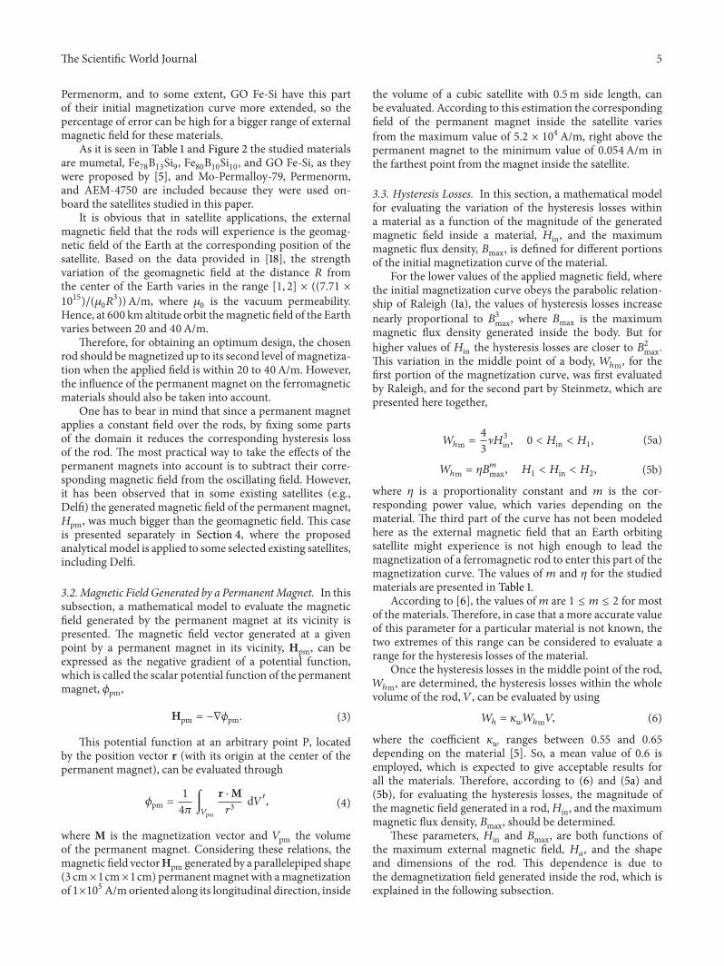
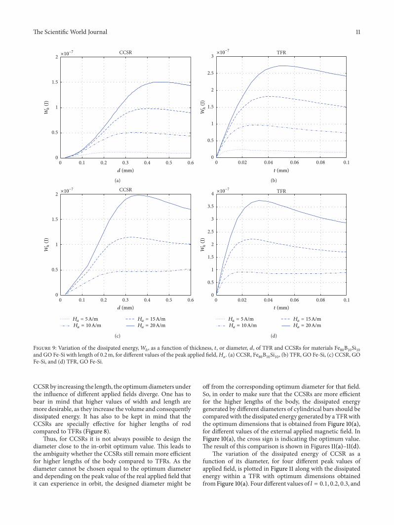

International Journal of
AerospaceEngineeringHindawi Publishing Corporationhttpwwwhindawicom Volume 2014
RoboticsJournal of
Hindawi Publishing Corporationhttpwwwhindawicom Volume 2014
Hindawi Publishing Corporationhttpwwwhindawicom Volume 2014
Active and Passive Electronic Components
Control Scienceand Engineering
Journal of
Hindawi Publishing Corporationhttpwwwhindawicom Volume 2014
International Journal of
RotatingMachinery
Hindawi Publishing Corporationhttpwwwhindawicom Volume 2014
Hindawi Publishing Corporation httpwwwhindawicom
Journal ofEngineeringVolume 2014
Submit your manuscripts athttpwwwhindawicom
VLSI Design
Hindawi Publishing Corporationhttpwwwhindawicom Volume 2014
Hindawi Publishing Corporationhttpwwwhindawicom Volume 2014
Shock and Vibration
Hindawi Publishing Corporationhttpwwwhindawicom Volume 2014
Civil EngineeringAdvances in
Acoustics and VibrationAdvances in
Hindawi Publishing Corporationhttpwwwhindawicom Volume 2014
Hindawi Publishing Corporationhttpwwwhindawicom Volume 2014
Electrical and Computer Engineering
Journal of
Advances inOptoElectronics
Hindawi Publishing Corporation httpwwwhindawicom
Volume 2014
The Scientific World JournalHindawi Publishing Corporation httpwwwhindawicom Volume 2014
SensorsJournal of
Hindawi Publishing Corporationhttpwwwhindawicom Volume 2014
Modelling amp Simulation in EngineeringHindawi Publishing Corporation httpwwwhindawicom Volume 2014
Hindawi Publishing Corporationhttpwwwhindawicom Volume 2014
Chemical EngineeringInternational Journal of Antennas and
Propagation
International Journal of
Hindawi Publishing Corporationhttpwwwhindawicom Volume 2014
Hindawi Publishing Corporationhttpwwwhindawicom Volume 2014
Navigation and Observation
International Journal of
Hindawi Publishing Corporationhttpwwwhindawicom Volume 2014
DistributedSensor Networks
International Journal of