Research Article An Integrated Conceptual Framework for ...

Research ArticleAn Integrated Conceptual Framework for Adapting ForestManagement Practices to Alternative Futures

Tony Prato1 and Travis B. Paveglio2

1 Department of Agricultural and Applied Economics, University of Missouri, Columbia, MO 65211, USA2Department of Conservation Social Sciences, University of Idaho, Moscow, ID 83844, USA

Correspondence should be addressed to Tony Prato; [email protected]

Received 19 September 2013; Accepted 22 January 2014; Published 12 March 2014

Academic Editor: Hubert Sterba

Copyright © 2014 T. Prato and T. B. Paveglio. This is an open access article distributed under the Creative Commons AttributionLicense, which permits unrestricted use, distribution, and reproduction in any medium, provided the original work is properlycited.

This paper proposes an integrated, conceptual framework that forestmanagers can use to simulate themultiple objectives/indicatorsof sustainability for different spatial patterns of forest management practices under alternative futures, rank feasible (affordable)treatment patterns for forested areas, and determine if and when it is advantageous to adapt or change the spatial pattern over timefor each alternative future.The latter is defined in terms of three drivers: economic growth; land use policy; and climate change. Fourforestmanagement objectives are used to demonstrate the framework,minimizingwildfire risk andwater pollution andmaximizingexpected net return from timber sales and the extent of potential wildlife habitat. The fuzzy technique for preference by similarityto the ideal solution is used to rank the feasible spatial patterns for each subperiod in a planning horizon and alternative future.Theresulting rankings for subperiods are used in a passive adaptivemanagement procedure to determine if and when it is advantageousto adapt the spatial pattern over subperiods. One of the objectives proposed for the conceptual framework is simulated for theperiod 2010–2059, namely, wildfire risk, as measured by expected residential losses from wildfire in the wildland-urban interfacefor Flathead County, Montana.

1. Introduction

Maintaining the long-term sustainability of forest ecosys-tems is challenging due to uncertainty about future changesin socioeconomic, biophysical, and other conditions thatinfluence the achievement of forest management objectives.Several studies have proposed management strategies toenhance the capacity of forest ecosystems to respond oradapt to new or changing conditions or, equivalently, toincrease the resilience of forest ecosystems to change [1–6]. Most studies of this sort focus on how changes in justone condition influence a particular management objective(e.g., how landscape fragmentation resulting from residentialdevelopment degrades wildlife habitat or how increases intemperature resulting from climate change influence thedistribution of tree species). Few studies have assessed howmultiple socioeconomic, biophysical, and other conditionsinfluence the multiple objectives for which many forests are

managed. This deficiency may be due, in part, to the lack ofan integrated conceptual framework that forest managers canuse to evaluate the impacts ofmultiple conditions onmultipleforest management objectives and how best to adapt forestmanagement practices to uncertain future changes in thoseconditions.

This paper proposes an integrated conceptual frameworkfor that purpose. The framework: (1) simulates the multipleobjectives achieved by different spatial patterns of forestmanagement practices (or patterns for short) under alterna-tive economic growth, land use policy, and climate changefutures; (2) ranks feasible patterns for areas managed bydifferent forest managers; and (3) determines if and whenit is advantageous for a forest manager to adapt or changethe pattern over time in response to economic growth andchanges in land use policy and climate. Empirical resultsare presented for one of the objectives proposed for theframework.

Hindawi Publishing CorporationInternational Journal of Forestry ResearchVolume 2014, Article ID 321345, 13 pageshttp://dx.doi.org/10.1155/2014/321345

2 International Journal of Forestry Research

Forest management

objectives

Fire behavior, water pollution, and wildlife

habitat simulation models

Land ownershipand pixel/parcel

locationsSimulation of

residential development

Alternative futures (economic growth, land use policy, and

climate changescenarios)

Fuzzy TOPSIS decision model

and ratingsForest management practices and feasible

patterns

Most preferred spatial patterns of forest management

practicesAdaptation of

feasible patterns to alternative futures

Structure and land values

Figure 1: Flow diagram of proposed conceptual framework.

2. Proposed Framework

This section begins with an overview of the proposed frame-work (see Figure 1) followed by detailed descriptions of thesubmodels for that framework. The framework evaluatesspatial patterns of forest management practices in terms offour objectives (1) expected residential losses due to wildfire(E(RLW)), or wildfire risk; (2) water pollution; (3) expectednet return from timber sales; and (4) extent of potentialwildlife habitat. Several submodels and assumptions areused to simulate E(RLW). Future residential developmentis simulated using the RECID2 land use change simulationmodel. Input for that model includes the amount of landrequired for new residential development, which is simulatedusing the impact analysis for planning (IMPLAN) regionaleconomic model in combination with the growth rates foreconomic sectors specified by the economic growth scenarioand assumptions about the location and density of newresidential development as specified in the land use policyscenario. Changes in vegetation over time are simulated usingthe FireBGCv2 model, which requires inputting temperatureand precipitation projections corresponding to a particularclimate change scenario, information on current vegetation,landownership patterns, and forest management practicesused by landowners. Vegetation changes over time areinputted to the FSimmodel to estimate burn probabilities fora forested landscape and conditional probabilities of variousflame length categories for smaller areas of the landscape.Several models can be used to simulate water pollution andextent of potential wildlife habitat for different spatial pat-terns of forest management practices. Estimation of expectednet return from timber sales is relatively straightforward oncethe volume of timber harvested andmarket prices for logs hasbeen determined.Themost preferred spatial patterns of forestmanagement practices are determined by ranking feasiblespatial patterns of forest management practices using thesimulated values of the four management objectives for thosepatterns in a multiple attribute evaluation method (i.e., fuzzytechnique for preference by similarity to the ideal solution-fuzzy TOPSIS).

Because each of the four objectives depends on a largenumber of parameters and assumptions, it is infeasible to

conduct a sensitivity analysis with respect to all the possiblecombinations of those parameters and assumptions. Further-more, there is little basis for choosing which combinations ofparameters/assumptions to include in a sensitivity analysis.For those reasons, it is not feasible to analyze how sensitivethe preferred spatial pattern of forest management practicesfor a landscape is to the parameters and assumptions ofthe framework. Instead, the focus is placed on groundingthe assumptions and inputs used in submodels to accuratelyrepresent the socioecological landscape being studied (e.g.,see the description of methods used to derive data for thesimulation of E(RLW) [7] or the RECID2 model [7, 8]).The alternative futures analysis described in the next sectiondoes allow users to evaluate how sensitive the objectives andpreferred spatial pattern of forest management practices areto different alternative futures (i.e., different combinationsof economic growth, land use policy, and climate changescenarios). For example, the sensitivity of E(RLW) to threedifferent land use policies has been evaluated [7].

2.1. Alternative Futures Analysis. The conceptual frameworkuses alternative futures analysis (AFA) to account for uncer-tainty regarding future economic growth, land use policy,and climate change. AFA has been used in several studiesconducted in several areas of North America, includingPennsylvania [9], California [10], the Willamette River Basinin Oregon [11, 12], the Upper San Pedro River Basin inArizona and Sonora, Mexico [13], Wisconsin [14], and Flat-head County, Montana [7]. AFA rests on three premises:(1) decision-makers and stakeholders are unsure about whatthe future will bring (i.e., there is uncertainty); (2) no singlevision of the future is likely to be accurate or superior to allothers; and (3) impacts of future change need to be evaluatedfor a range of conditions [13]. AFA does not predict futureoutcomes. Rather, it evaluates possible future outcomes underparticular assumptions.

In this study, an alternative future consisted of a particularcombination of an economic growth scenario, land use policyscenario, and climate change scenario for each subperiod inthe planning horizon. For example, if the planning horizonis 2014–2063 (50 years) and the subperiods are 10 years long,there are five subperiods: 2014–2023; 2024–2033; 2034–2043;2044–2053; and 2054–2063. An alternative future is the samethroughout the planning horizon.

An economic growth scenario specifies the averageannual growth rate over the planning horizon for eacheconomic sector of the regional economy within which theforests of interest are located. Economic growth in each sectorcreates new jobs.New jobs are converted into newhouseholdsand new households require housing units to live in and landon which to build those housing units. The number of newjobs associated with a particular growth rate is projected foreach subperiod using the IMPLAN regional economic anal-ysis model [15]. The number of new households associatedwith the number of new jobs is estimated by multiplyingthe new jobs by a population-to-jobs ratio and dividing bythe average persons per household. The resulting increase inhouseholds is multiplied by a housing units-to-households

International Journal of Forestry Research 3

ratio to estimate the increase in housing units associatedwith a particular growth rate. The amount of additional landrequired for additional housing units is determined using theRECID2 model described below.

A land use policy scenario specifies: (1) the percentageof housing units in each of six residential housing densityclasses; (2) setbacks of houses from wetlands and water-bodies; (3) the type and density of residential developmentallowed in environmentally sensitive areas (i.e., wetlands,streams, rivers, lakes, ponds, and shallow aquifers) andwithinand outside of sewer accessible areas; and (4) for example, nodevelopment on most public land, on parcels in the 100-yearfloodplain, and on parcels that have an average slope greaterthan 30%. As the land use policy scenario becomes morerestrictive, the density of houses and setbacks from wetlandsand waterbodies increases and the type of developmentallowed in environmentally sensitive areas becomes morelimited. For all three land use policy scenarios, only high,urban, and suburban density housing are allowed on sewer-accessible parcels; rural, exurban, and agricultural densityhousing are allowed on all developable parcels. The sixresidential density classes and corresponding number ofhousing units per developed hectare are: (1) high (15.56–19.02); (2) urban (12.23–14.94); (3) suburban (3.71–6.18); (4)rural (1.85–3.09); (5) exurban (0.25–0.40); and agricultural(0.040–0.064). The sizes of developed parcels in a residentialdensity class are randomly selected from the ranges of parcelsizes for that density class.

The RECID2 model uses the requirement for additionalhousing units in each density class, the number and sizeof parcels available for new residential development, anddevelopment attractiveness scores for developable parcelsto determine on which parcels in the WUI to place newresidences during each subperiod. More details about theRECID2 model are given by Prato et al. [8].

The economic growth and land use policy scenarios for asubperiod influence the spatial extent of the wildland-urbaninterface (WUI), the number and density of homes in theWUI, and expected residential losses from wildfire for thatsubperiod. A WUI is the area where residential structuresare adjacent to or interspersed with wildland vegetation [16,17]. Expected residential losses from wildfire are the wildfirerisk metric used in the decision model for the conceptualframework.

Uncertainty regarding future CO2mitigation, nonlinear

thresholds in the climate system, and limitations of thecurrent generation of climate models leads to uncertaintyabout future climate change. Such uncertainty influencesvegetative growth, forest succession, and the probability ofwildfire in a forested landscape. Climate scenarios and asso-ciated projections of temperature and precipitation, whichare input to the biophysical models (i.e., FireBGCv2 andFSim), are obtained from the International Panel on ClimateChange (IPCC)’s fourth assessment [18] or fifth assessment[19]. To apply the IPCC emission scenarios to a forestedlandscape at the local level (e.g., at the spatial scale of anational forest), requires spatial and temporal downscalingof the IPCC projections of temperature and precipitationfor each emission scenario. Currently, the World Climate

Research Program’s (WCRP’s) Coupled Model Intercompar-ison Project Phase 5 (CMIP5) [20] provides 12 km2 res-olution temperature and precipitation projections for theA1B, A2, and B1 emission scenarios. The CMIP data arebias corrected (monthly means adjusted and matched to theobservational climate data) and validated against observa-tional data using the two-step process described by Woodet al. [21, 22] and Meehl et al. [23]. Because the biophysicalmodels require daily temperature and precipitation data,the CMIP projections are downscaled to daily tempera-ture and precipitation projections using the delta method[7, 24].

2.2. Decision Model. The decision model uses fuzzy TOPSISto rank the feasible patterns for each subperiod and alter-native future. A pattern specifies which forest managementpractice (e.g., commercial harvesting, mechanical thinning,or prescribed burning) to apply to each pixel managed by aforest manager. A spatial pattern for a subperiod is feasibleif total expenditures on forest management practices forthat pattern do not exceed the manager’s expected budgetfor forest management practices for that subperiod. Spatialvariability in the biophysical characteristics of pixels anddifferences in the relative importance of objectives acrossforest managers could cause the ranking of patterns to varyacross forest managers. For example, in terms of the relativeimportance of objectives, the Multiple Use and SustainedYieldAct of 1960 requires theUSDAForest Service tomanagetheir lands for outdoor recreation, range, timber, watershed,and fish, and wildlife with no use greater than any other (i.e.,the five uses or objectives are equally important). In contrast,the primary management objective of a private industrialforest manager is to maximize net return from the sale oflogs subject to constraints, such as legally mandated bestmanagement practices.

Fuzzy TOPSIS is a fuzzy multiple objective decisionmethod that ranks decision alternatives based on theircloseness coefficients [25–28]. The latter indicate how closethe values of the objectives for a feasible pattern are to thevalues of the objectives for the fuzzy positive-ideal patternand how far away they are from the values of the objectivesfor the fuzzy negative-ideal pattern. The fuzzy positive-idealpattern has themost desirable values of the objectives and thefuzzy negative-ideal pattern has the least desirable values ofthe objectives.

Advantages of fuzzy TOPSIS are that, unlike the utilityfunction approach to ranking decision alternatives [29, 30],it does not assume utility independence for objectives anda risk-neutral decision-maker. Utility independence impliesthat the marginal utility of one objective is independent ofthe amounts of all other objectives. A risk-neutral decision-maker compares and ranks alternatives based solely on theirexpected values.

Application of fuzzy TOPSIS requires: (1) determiningwhich objectives are positive (i.e., more is preferred to lessof the objective) or negative (i.e., less is preferred to moreof the objective); and (2) selecting narrative descriptions orlinguistic variables for both the values of the management


objectives and their relative importance. For example, sup-pose patterns are characterized in terms of four managementobjectives: wildfire risk; water pollution; net return from thesale of wood products; and extent of potential wildlife habitat.Wildfire risk and water pollution are negative objectives andthe sale of wood products and extent of potential wildlifehabitat are positive objectives.

In order to rank patterns using fuzzy TOPSIS, forestmanagers must first rate the simulated values and the relativeimportance of the attributes. A convenient way to do suchratings is to assign triangular fuzzy numbers to the linguisticvariables used in the ratings. A triangular fuzzy number isdesignated as 𝑇(𝑎, 𝑏, 𝑐), or simply (𝑎, 𝑏, 𝑐), where 𝑎 is theminimum value, 𝑏 is the mode, and 𝑐 is the maximum valueof the triangular probability distribution (Figure 2).

Table 4 is an example of assigning triangular fuzzy num-bers to linguistic variables for rating the simulated values ofobjectives.

Similarly, Table 5 is an example of how to assign triangu-lar fuzzy numbers to linguistic variables for rating the relativeimportance of objectives.

The triangular fuzzy numbers appearing in Tables 4 and5 are variants of the ones proposed by Chen [27].

Ratings of the values and relative importance of attributescan be done by either individual members of a managementteam or the team as a whole. If ratings are done by indi-vidual members, then the fuzzy numbers corresponding tothe linguistic variables assigned by individual members areaveraged to obtain fuzzy numbers for the management team.For example, if the triangular fuzzy numbers correspondingto the linguistic variables assigned to a particular attributeby the first and second member of the management teamare (𝑎

(1)

𝑖𝑗, 𝑏(1)

𝑖𝑗, 𝑐(1)

𝑖𝑗) and (𝑎

(2)

𝑖𝑗, 𝑏(2)

𝑖𝑗, 𝑐(2)

𝑖𝑗), respectively, then the

average triangular fuzzy number for the attribute (i.e., (𝑎(1)𝑖𝑗

+

𝑎(2)

𝑖𝑗)/2, (𝑏(1)

𝑖𝑗+ 𝑏(2)

𝑖𝑗)/2, (𝑐

(1)

𝑖𝑗+ 𝑐(2)

𝑖𝑗)/2) is used in the fuzzy

TOPSIS. If the assignment of linguistic variables is done bythe management team as a whole, then the fuzzy numberscorresponding to those assignments are used in the fuzzyTOPSIS.

If there are 𝑛𝑡feasible spatial patterns for subperiod 𝑡, then

the fuzzy TOPSIS ranks those patterns based on the followingcloseness coefficients:

𝐶𝑖=

𝑑−

𝑖

𝑑+

𝑖+ 𝑑−

𝑖

(0 ≤ 𝐶𝑖≤ 1, 𝑖 = 1, . . . , 𝑛

𝑡) , (1)

where 𝑑+

𝑖is the vertex distance between pattern 𝑖 and the

positive-ideal solution (V+𝑗), and 𝑑

−

𝑖is the vertex distance

between pattern 𝑖 and the negative-ideal solution (V−𝑗). Vertex

distances are calculated as follows:

𝑑+

𝑖=

4

∑

𝑗=1

𝑑 (𝑤𝑗𝑟𝑖𝑗, V+𝑗) ,

𝑑−

𝑖=

4

∑

𝑗=1

𝑑 (𝑤𝑗𝑟𝑖𝑗, V−𝑗) .

(2)

T(a,b,c)

0 a b c

Figure 2: Triangular fuzzy number.

𝑑(⋅) is the vertex distance operator. For example, 𝑑(𝑤𝑗𝑟𝑖𝑗, V+𝑗)

is the vertex distance between the weighted normalizedfuzzy effect of pattern 𝑗 on objective 𝑖 and the positive-ideal solution. For two fuzzy numbers, 𝑧

1= (𝑒

1, 𝑒2)

and 𝑧2

= (𝑘1, 𝑘2), the vertex distance is 𝑑(𝑧

1, 𝑧2) =

{0.33[(𝑒1− 𝑘1)2+ (𝑒2− 𝑘2)2]}0.5. For the four attributes con-

sidered here, V+𝑗

= (0, 0) and V−𝑗

= (1, 1) for wildfire riskand water pollution and V+

𝑗= (1, 1) and V−

𝑗= (0, 0) for

net return from the sale of wood products and the extent ofpotential wildlife habitat. The closer (or farther away) 𝐶

𝑖is to

(or from) one, the more desirable (or less desirable) is pattern𝑖. Closeness coefficients are used to rank feasible patternsfrom most desirable to least desirable in descending orderof their closeness coefficients. The preferred feasible patternfor a forest manager is the one whose closeness coefficient isnearest to one. For an application of fuzzy TOPSIS, see Prato[31, 32].

2.3. Simulating Objectives. This section describes the proce-dures used to simulate the four objectives considered here.Because there has been considerable research on evaluatingthe impacts of forest management practices on water qualityand the extent of potential wildlife habitat, simulation of netreturn is relatively straightforward, and little research hasbeen done on simulating wildfire risk; the explanation of theprocedures used to simulate wildfire risk is more extensivethan the explanations of the procedures used to simulatewater quality, extent of potential wildlife habitat, and netreturn.

2.3.1. Wildfire Risk. Wildfire risk is defined as expectedresidential losses from wildfire in the WUI or E(RLW) forshort. E(RLW) is simulated at the spatial scale of individualresidential properties. That choice of spatial scales allowsE(RLW) to be aggregated to larger spatial scales, such asneighborhoods or theWUI as awhole. Simulation of E(RLW)requires information about: (1) housing units that exist at thebeginning of the planning horizon (i.e., existing residentialproperties); (2) number of new housing units added in eachsubperiod; (3) location and density of new housing units; (4)effects of climate change on growth in forest vegetation andburn probabilities for residential properties; (5) residentialhomeowners’ choices regarding vegetation management in


the Home Ignition Zone (HIZ) and building materials usedin residential structures; and (6) spatial extent of the WUI.

E(RLW) for the WUI is defined as

E (RLW) = E𝑑(RLW) + E

𝑤(RLW) , (3)

where E𝑑(RLW) is present value in the base year of E(RLW)

for existing residential properties and E𝑤(RLW) is present

value in the base year of E(RLW) for new residential prop-erties added during the planning horizon.

The base year is the first year in the planning horizon.E𝑑(RLW) is defined as

E𝑑(RLW) = PV

𝑏[E𝑑1(RLW) ,E

𝑑2(RLW) ,

E𝑑3(RLW) ,E

𝑑4(RLW) ,E

𝑑5(RLW)] ,

(4)

where PV𝑏stands for present value in the base year. E

𝑑𝑡(RLW)

is undiscounted expected wildfire losses for existing residen-tial properties during subperiod 𝑡 defined as

E𝑑𝑡(RLW)

=

𝑚𝑑

∑

𝑗=1

pb𝑗𝑡[(

𝑛𝑑𝑗

∑

ℎ=1

pSℎ𝑗𝑡VS𝑑ℎ𝑗𝑡

) + 𝛽𝑗𝑡TV𝑑𝑗𝑡] ,

(5)

where 𝑚𝑑is the number of parcels in the WUI containing

existing residential properties; 𝑛𝑑𝑗is the number of existing

residential properties in parcel 𝑗; pb𝑗𝑡is the probability that

parcel 𝑗 burns during subperiod 𝑡; pSℎ𝑗𝑡

is the probability thatstructures on property ℎ in parcel 𝑗 burn during subperiod𝑡 given parcel 𝑗 burns during subperiod 𝑡; is the total valueof existing structure(s) on residential property ℎ in parcel 𝑗during period 𝑡; 𝛽

𝑗𝑡is the average percentage loss in aesthetic

value of residential properties in parcel 𝑗 during subperiod𝑡 given parcel 𝑗 burns during subperiod 𝑡; and TV

𝑑𝑗𝑡is the

total value of each existing residential property (structure andland) in parcel 𝑗 during subperiod 𝑡.

𝑛𝑑𝑗

is determined using computer-assistedmass appraisal(CAMA) data or similar data for the WUI. CAMA dataare typically used to keep track of property values andassessments and determine annual property taxes. pbjt issimulated using the FireBGCv2 and FSim models [33, 34].FireBGCv2 simulates future changes in forest vegetation forforest stands in the area of interest under a particular climatechange scenario and themanagement practices typically usedby landowners. The FSim model uses the outputs of theFireBGCv2 model to estimate burn probabilities for 90m2pixels in a forested landscape and conditional probabilities ofvarious flame length categories given pixel burns.

pSℎ𝑗𝑡

is simulated using the procedures described by Pratoet al. [35]. VS

𝑑ℎ𝑗𝑡is the total value of all existing structures or

buildings located on residential property ℎ in parcel 𝑗 duringsubperiod 𝑡. It is estimated by VS

𝑑ℎ𝑗𝑡= (1 + 𝜆)

𝑞 VS𝑑ℎ𝑗𝑜

,where VS

𝑑ℎ𝑗𝑜is the total value of existing structures located

on residential property ℎ in parcel 𝑗 in the first year of theplanning horizon determined from the CAMA (or similar)data for that year. 𝜆 is the assumed annual average growth inproperty values in the WUI over the planning horizon.

𝛽𝑗𝑡is estimated using research results from Stetler et al.

[36] on aesthetic property values and reductions in propertyvalues following wildfire, information about wildfire impactson property values obtained from property assessors, and theflame length outputs of the FSimmodel [34, 37]. A geographicinformation system (GIS) is used to derive weighted averageflame length intensities for parcels and determine one of fourfixed amounts of aesthetic property value losses given theaverage flame length for that parcel [35]. TV

𝑑𝑗𝑡is simulated

by TV𝑑𝑗𝑡

= (1 + 𝜆)𝑞TV𝑑𝑗𝑜

, where TV𝑑𝑗𝑜

is the sum ofthe assessed building and land values for existing residentialproperties located on parcel 𝑗 at the beginning of the planninghorizon, and 𝜆 and 𝑞 are defined above. (pS

ℎ𝑗𝑡)(VS𝑑ℎ𝑗𝑡

) isexpected wildfire-related loss in the value of the existingstructures located on residential property ℎ in parcel 𝑗

during subperiod 𝑡. (𝛽𝑗𝑡)(TV𝑑𝑗𝑡) is expected wildfire-related

loss in the aesthetic value of existing residential properties(including structures and land) located on parcel 𝑗 duringsubperiod 𝑡 given parcel 𝑗 burns during period 𝑡.

E𝑤(RLW) is defined as

E𝑤(RLW) = PV

𝑏[E(1)𝑤

(RLW) ,E(2)𝑤

(RLW) ,E(3)𝑤

(RLW) ,

E(4)𝑤

(RLW) ,E(5)𝑤

(RLW)] ,

(6)

where E(𝑡)𝑤(RLW) is the present value in the base year of

expected wildfire losses during the planning horizon for newresidential properties added during subperiod 𝑡. It is definedas

E(𝑡)𝑤(RLW) = PV

𝑡[E𝑤𝑡(RLW) + ⋅ ⋅ ⋅ + E

𝑤(𝑡+𝑘)(RLW)] , (7)

where PV𝑡is the present value at the end of subperiod 𝑡, 𝑘

equals 4 for 𝑡 = 1 (first subperiod), 3 for 𝑡 = 2 (secondsubperiod), 2 for 𝑡 = 3 (third subperiod), and so forth.E𝑤𝑡(RLW) is E(RLW) at the end of subperiod 𝑡 for new

residential properties added during subperiod 𝑡. E𝑤𝑡(RLW)

is defined as

E𝑤𝑡(RLW) =

𝑚𝑤𝑡

∑

𝑗=1

pb𝑗𝑡[(

𝑛𝑤𝑗𝑡

∑

ℎ=1

pSℎ𝑗𝑡VS𝑤ℎ𝑗𝑡

) + 𝛽𝑗𝑡TV𝑤𝑗𝑡

] ,

(8)

where𝑚𝑤𝑡

is the number of parcels in theWUI in which newresidential properties are added during subperiod 𝑡; 𝑛

𝑤𝑗𝑡is

the number of new residential properties added to parcel 𝑗during subperiod 𝑡; pb

𝑗𝑡is the probability that parcel 𝑗 burns

during subperiod 𝑡; pSℎ𝑗𝑡

is the probability that structures onproperty ℎ in parcel 𝑗 burn during subperiod 𝑡 given parcel𝑗 burns during subperiod 𝑡; VS

𝑤ℎ𝑗𝑡is the total value of new

structures added to residential property ℎ in parcel 𝑗 duringsubperiod 𝑡; 𝛽

𝑗𝑡is the average percentage of loss in aesthetic

value of residential properties in parcel 𝑗 during subperiod 𝑡

given parcel 𝑗 burns during subperiod 𝑡; and TV𝑤𝑗𝑡

is the totalvalue of structures and land for a new residential propertyadded to parcel 𝑗 during subperiod 𝑡.

𝑛𝑤𝑘𝑡

is determined using the RECID2 model describedin Section 2.1. Other parameters in (8) are estimated using


procedures similar to the ones used to estimate the corre-sponding parameters in (1). VS

𝑤ℎ𝑗𝑡and TV

𝑤𝑗𝑡are simulated

using a linked geospatial database of existing property andstructure values stratified across neighborhoods in the WUI.Each new residential property added during a subperiod isassigned an appreciated value for the structure(s) on thatproperty and a per hectare land value. Both structure and perhectare land values are drawn randomly from either water-front or nonwaterfront properties in the same neighborhoodwithin a WUI.

2.3.2.Water Pollution. Different forestmanagement practicesleave different amounts of vegetative cover on a landscape,which influence the runoff rates to waterbodies locateddownslope of that landscape. For example, commercialharvesting is likely to cause higher soil erosion rates andsedimentation of downslope waterbodies than mechanicalthinning. Sediment loads to waterbodies affect the qualityof habitat for aquatic species. In addition, water pollutionis influenced by the amount and timing of runoff, which isinfluenced by climate change.

Several biophysical models can be used to simulate waterquality for different land uses or land covers. For example,the Soil and Water Assessment Tool (SWAT) was used tosimulate the effects of forest management practices on waterhydrology, water quality, and ecosystem services [38, 39].Using SWAT to simulate the impacts of forest managementpractices and climate change on water quality requires delin-eating watersheds and running SWAT for each watershed.

2.3.3. Expected Net Return. Expected net return for a patternequals the expected total revenue from selling the marketablebiomass removed by the forest management practices thatmake up that pattern, if any, minus the cost of the forestmanagement practices for that pattern. Calculating expectednet return requires projecting wood product prices andcosts of forest management practices for each subperiod.Wood product prices are market determined and unlikelyto vary across forest managers. The cost of a pattern is thesum, overall management practices used in that pattern,of the product of cost per hectare of a forest managementpractice and the number of hectares to which that practiceis applied. Per hectare costs are likely to vary across pixels,even for the same practice, due to spatial variability in slope,aspect, initial forest biomass, forest biomass removed, newroad construction and hauling distances (if any), labor andequipment requirements, and other factors. The cost of apattern is estimated using models, such as the harvest costmodel [40].

2.3.4. Extent of Potential Wildlife Habitat. Different patternsof forest management practices and climate projections arelikely to have different effects on the extent of potentialhabitat for wildlife species. For example, forest managementpractices that open up the forest canopy allow more sunlightto reach the forest floor, which stimulates production ofgrasses and shrubs and improves habitat for herbivores, suchas deer and elk. Open logging roads in prime habitat areas

for grizzly bear increase interactions between humans andgrizzly bear, which tends to increase grizzly bear mortality[2]. Projected changes in temperature and precipitationcorresponding to different climate change scenarios can havepositive or negative impacts on the extent of potential wildlifehabitat depending on the species [41].

Effects of the spatial pattern of forest management prac-tices and climate change on the extent of potential wildlifehabitats can be evaluated by combining land cover/land usedata or landscape metrics for each pattern, temperature andprecipitation projections for each climate change scenario,and species distribution and persistence models for vari-ous species (e.g., [1, 42, 43]). Landscape metrics can becalculated using computer programs such as FRAGSTATS[44] or APACK [45]. For example, Thoma and Shovic [46]assessed the potential impacts of future climate change onthree species by identifying spatial habitat characteristics andextent of present-day occurrence of the species, using thelapse rate to predict elevations that are likely to providefavorable temperatures for the species in 2100 (based onclimate projections for the IPCC A2 and B1 emission scenar-ios), employing species distribution and persistence modelsto map the resulting extent of current and future potentialhabitat for the species and comparing the two extents todetermine whether the extent of potential habitat for thespecies increases or decreases.

2.4. Rating Values and Relative Importance of Objectives.Application of fuzzy TOPSIS requires each member of aforest management team or the team as a whole to ratethe simulated values and relative importance of objectivesusing linguistic variables. The task of rating the relativeimportance of objectives using linguistic variables is relativelystraightforward. However, the task of rating simulated valuesof the objectives can be onerous, especially when there arenumerous feasible patterns and/or management objectives.Rating of objectives can be simplified by asking eachmemberof a management team or the team as a whole to: (1) consideran index number for the simulated values of each objectivewhere the range of the index number is [0, 100]; and (2) dividethe range for each objective into nonoverlapping intervalswhere each interval represents a unique linguistic variable(e.g., 0–35 is very low, 36–55 is low, 56–75 is medium, 71–85 is high, and 86–100 is very high). Intervals can varyacross objectives and individualmembers of themanagementteam. The intervals are used to assign linguistic variables tosimulated values of objectives. For example, if the simulatedvalue of E(RLW) is 75 for a particular pattern, then E(RLW)for that pattern is high based on the intervals defined above.Once linguistic variables have been assigned to the simulatedvalues of all objectives and their relative importance, they areassigned to triangular fuzzy numbers using schemes such asthe ones given in Section 2.2.

2.5. Adaptive Management. AM postulates that if humanunderstanding of nature is imperfect, then human interac-tions with nature (e.g., application of forest managementpractices) should (ideally) be experimental [47]. Kohm and


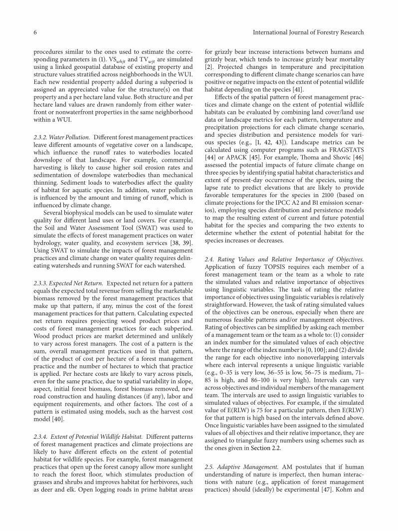
Table 1: Simulated subperiod areas of parcels required for and converted to six residential housing density classes, Flathead County,Montana,in hectares.

Housing density class Subperiod2010–2019 2020–2029 2030–2039 2040–2049 2050–2059

RequiredHigh 61 67 74 82 92Urban 78 85 94 105 117Suburban 351 384 424 470 525Rural 898 982 1,083 1,202 1,343Exurban 6,150 6,727 7,416 8,232 9,196Agricultural 29,363 32,119 35,408 39,306 43,908

ConvertedHigh 62 67 75 83 92Urban 78 88 95 105 118Suburban 354 385 433 473 778Rural 923 983 1,089 1,203 1,357Exurban 6,163 6,734 7,425 8,234 9,199Agricultural 29,556 32,233 35,579 39,329 37,769

Table 2: Simulated number of WUI parcels, area of WUI parcels, number of WUI residential structures, and area of the WUI for FlatheadCounty, 2010 and five subperiods.

Subperiod Number ofWUI parcels

% changebetween

subperiods

Area of WUIparcels (ha)

% changebetween

subperiods

Number of WUIresidentialstructures

% changebetween

subperiods

Area of theWUI (ha)

% changebetween

subperiods2010 15,761 — 41,014 — 15,766 — 294,344 —2010–2019 16,463 4 67,820 65 20,368 29 307,434 42020–2029 17,099 4 88,034 30 25,055 23 323,563 52030–2039 17,786 4 121,413 38 30,007 20 359,329 112040–2049 18,439 4 164,947 36 35,246 18 402,689 122050–2059 19,117 4 202,410 23 42,071 19 426,353 62010–2059 3,356 — 161,396 — 26,305 — 132,009 —

Franklin state that adaptive management is the only logicalapproach under the circumstances of uncertainty and thecontinued accumulation of knowledge [48, page 2]. Theprimary source of uncertainty for the decision problemconsidered here is that forest managers do not know whichalternative future is most likely to occur (i.e., probabilitiescannot be assigned to alternative futures).

AM can be either passive or active. For the currentapplication, active AM would involve using statistically validexperiments to test hypotheses about how changes in eco-nomic growth, land use policy, and climate influence themanagement objectives achieved by different forest man-agement practices or patterns and determine the best wayto adapt forest management practices or patterns to thosechanges based on the results of the experiments. Althoughactive AM does and passive AM does not provide statisticallyreliable results, active AM is more difficult and expensive toapply than passive AM.

The proposed conceptual framework utilizes passive AMto determine if and when a forest manager should adapt

the pattern in response to economic growth, changes in landuse policy, and climate change. Passive AM requires a forestmanager to: (1) formulatemodels of how a forested ecosystemis likely to respond to certain exogenous variables; (2) selectthe preferred pattern for each subperiod based on themodels;and (3) determine whether to change or adapt the patternover subperiods. The first step involves using the FireBGCv2and FSim models to simulate fire behavior and burn proba-bilities for each climate change scenario and subperiod, usingRECID2 to simulate changes in residential development ineach subperiod for each economic growth/land use policyscenario, and fuzzy TOPSIS to rank the feasible patternsfor each subperiod and alternative future. Economic growth,land use policy, and climate change are treated as exogenousvariables because changes in these variables are determined,for the most part, by conditions over which local forestmanagers have little influence.

The second step involves selecting management objec-tives, rating the simulated values and relative importance ofthe objectives, and using fuzzy TOPSIS to rank the feasible


Table 3: Nominal and inflation-adjusted simulated total E(RLW)and weighted mean E(RLW) for residential properties in theFlathead County WUI, by subperiod.

Subperiod Total E(RLW) Percent increase Weighted meanE(RLW)

Nominal dollars2000–2009 1,836,816 0 1182010–2019 2,539,544 38 1252020–2029 6,050,600 138 2412030–2039 13,351,965 120 4442040–2049 27,761,390 62 6172050–2059 33,872,543 55 805

Inflation-adjusted dollars2000–2009 1,836,816 0 1182010–2019 1,938,584 6 952020–2029 4,234,429 117 1692030–2039 6,014,398 42 2002040–2049 7,503,927 24 2132050–2059 8,937,346 19 212

Table 4: Assignment of triangular fuzzy numbers to linguisticvariables for rating simulated value of objectives.

Linguistic variable Triangular fuzzy numbervery low (0, 0, 1)low (0, 1, 3)medium (3, 5, 7)high (7, 8, 9)very high (9, 10, 10)

Table 5: Assignment of triangular fuzzy numbers to linguisticvariables for rating relative importance objectives.

Linguistic variable Triangular fuzzy numbervery low (0, 0, 0.1)low (0, 0.1, 0.3)medium (0.3, 0.5, 0.7)high (0.7, 0.8, 0.9)very high (0.9, 1.0, 1.0)

patterns for each subperiod and alternative future. Thepreferred pattern for a subperiod and alternative future is thefeasible pattern with the highest rank.

The third step involves determining if and when it isadvantageous for a forest manager to adapt a pattern tochanges in the exogenous variables across subperiods. Toillustrate the third step, consider a forest manager that hasidentified five feasible patterns and fuzzy TOPSIS indicatesthat the preferred patterns for a particular alternative futureare pattern 2 in the first and second subperiods, pattern 1 inthe third and fourth subperiods, and pattern 5 in the fifthsubperiod.These results imply that the forest manager shouldundertake the following adaptations over subperiods: (1) usepattern 2 in the first two subperiods; (2) switch from pattern

2 to pattern 1 in the third subperiod; (3) continue pattern 1 inthe fourth period; and (4) switch from pattern 1 to pattern 5in the fifth subperiod.

3. Results

Only a portion of the conceptual framework proposed herehas been implemented, namely, simulation of the inputs toE(RLW) and the values of E(RLW) for the WUI in FlatheadCounty,Montana. Simulations were based on: (1) five, 10-yearsubperiods (2010–2019, 2020–2029, 2030–2039, 2040–2049,and 2050–2059) covering the planning horizon 2010–2059;(2) an economic growth scenario that assumes an annualaverage rate of growth of 2.2% for the Flathead economy;(3) a land use policy for Flathead County that existed in2010 and a distribution of new housing units among thesix residential density classes of high—3%, urban—18%,suburban—42%, rural—6%, and agricultural—12%; and (4)climate projections corresponding to the IPCC A2 emissionscenario [18]. Scenarios for economic growth, land use policy,and climate change were assumed to remain constant acrossthe five subperiods. The remainder of this section reportssubperiod simulation results for: (1) residential developmentin the WUI; (2) parcel burn probabilities; (3) four WUImetrics; and (4) E(RLW) for the entireWUI. Simulated areasof parcels required for and converted to the six residentialhousing density classes for each subperiod are given inTable 1.

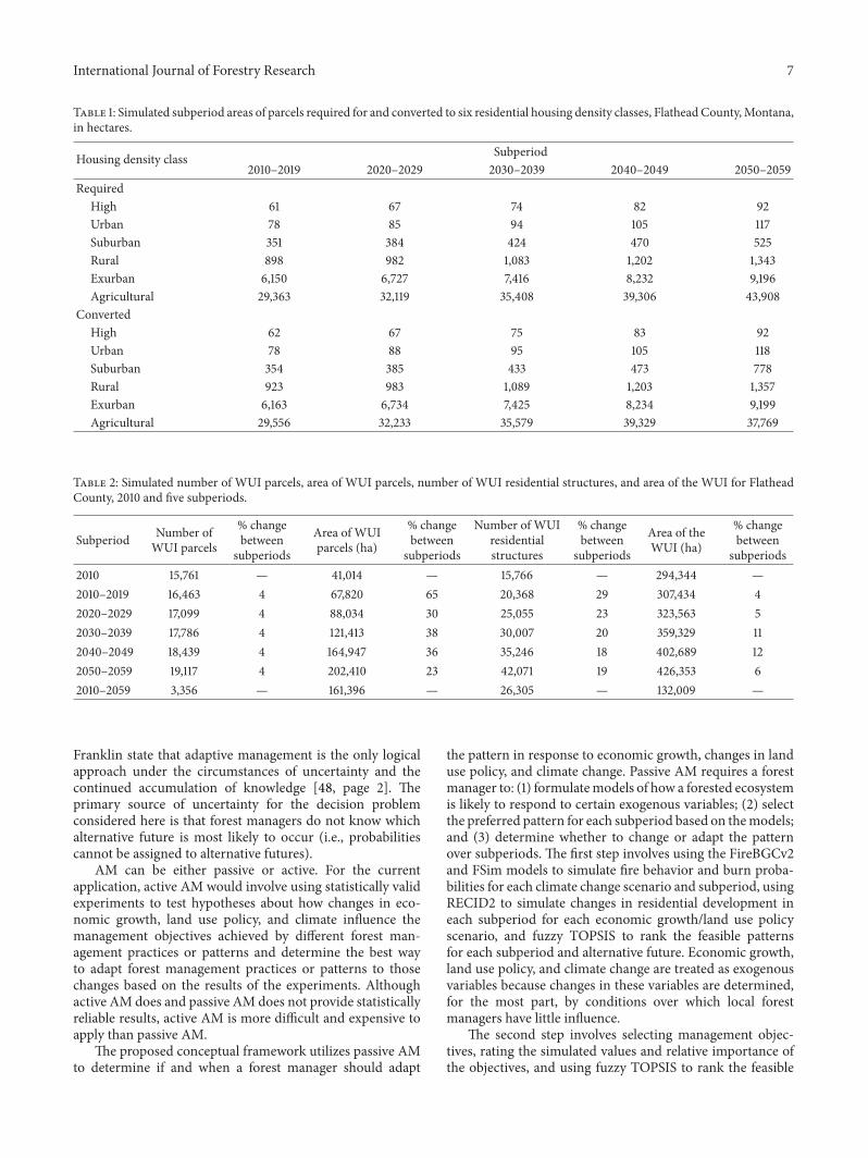
Figure 3 illustrates the simulated growth in residentialdevelopment for parcels in the WUI and the spatial extentof the WUI from 2010 to 2059 for Flathead County. Becauserural, exurban, and agricultural development occurs at rela-tively low densities, between 98% and 99% of the land areaconverted to new residential properties occurred at thosedensities. As expected, the area required for and convertedto residential development increases over subperiods. Areasrequired for and converted to residential housing are thesame (apart from differences caused by the discrete size ofparcels) for all housing density classes and subperiods exceptthe agricultural housing density class in the last subperiod. Inthat case, area required is 6,139 hectares greater than area con-verted because of the lack of developable parcels suitable forresidential development at the agricultural housing density.

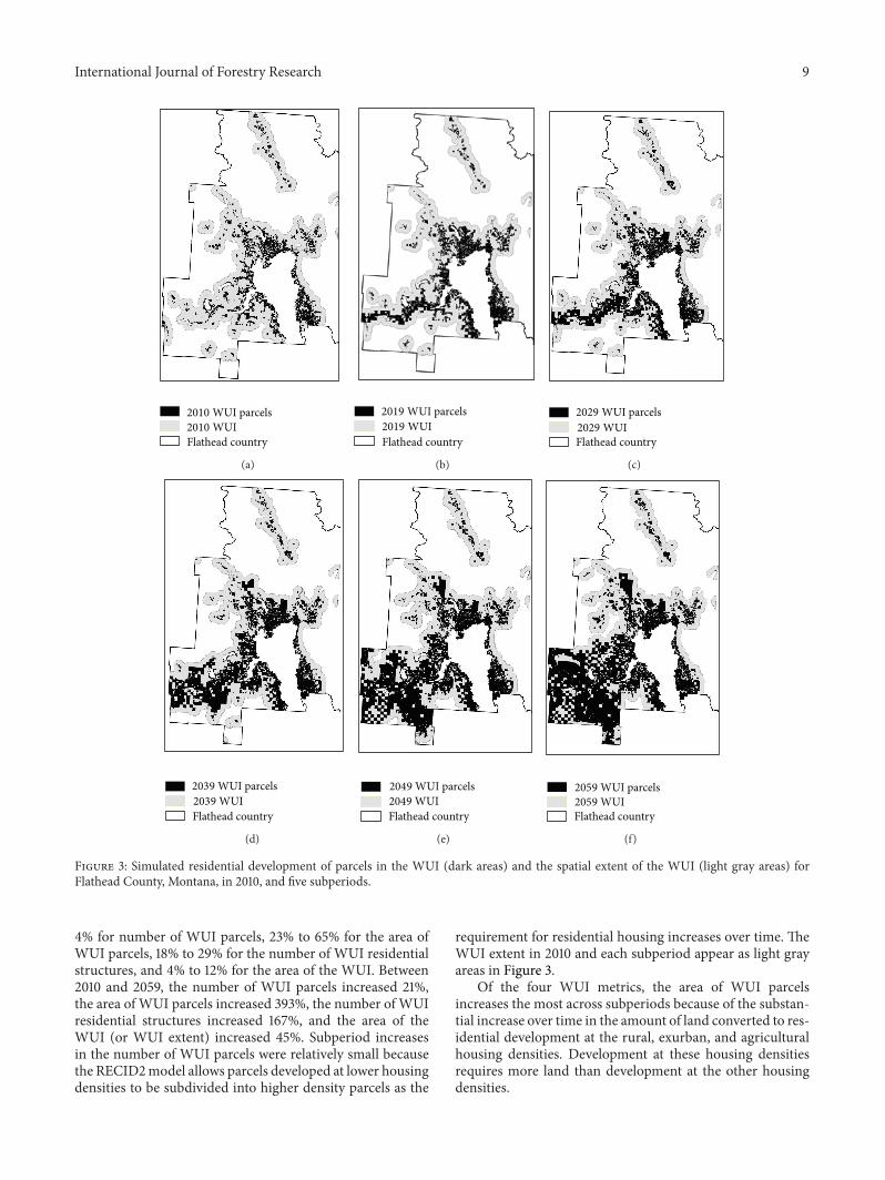
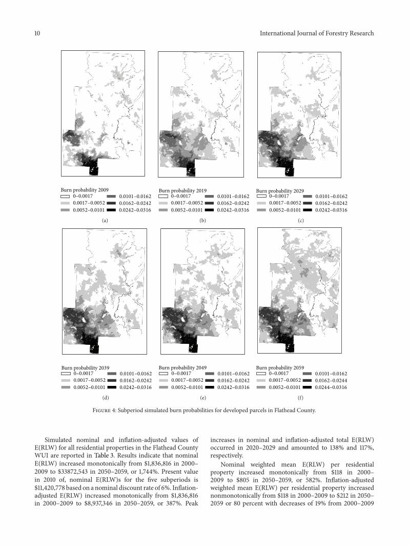
Burn probabilities for developed parcels for the five, 10-year subperiods ending in 2009, 2019, 2029, 2039, 2049, and2059 are illustrated in Figure 4. Parcel-level burn probabilitiesare highest and increase the most over subperiods in thesouthwest portion of the county. A greater proportion of thecounty is exposed to higher burn probabilities at the end(2059) than at the beginning (2010) of the planning horizon.For instance, burn probabilities for large areas in the northcentral portion of the county increase over subperiods. Ingeneral, there is considerable spatial and temporal variabilityin the magnitude of the parcel-level burn probabilities.

Table 2 contains the actual and simulated number ofWUIparcels, area of WUI parcels, number of WUI residentialstructures, and area of the WUI in 2010 and the five sub-periods. Subperiod increases in the four WUI metrics are


2010 WUI parcels2010 WUIFlathead country

(a)


(b)


(c)


(d)


(e)


(f)

Figure 3: Simulated residential development of parcels in the WUI (dark areas) and the spatial extent of the WUI (light gray areas) forFlathead County, Montana, in 2010, and five subperiods.

4% for number of WUI parcels, 23% to 65% for the area ofWUI parcels, 18% to 29% for the number of WUI residentialstructures, and 4% to 12% for the area of the WUI. Between2010 and 2059, the number of WUI parcels increased 21%,the area of WUI parcels increased 393%, the number of WUIresidential structures increased 167%, and the area of theWUI (or WUI extent) increased 45%. Subperiod increasesin the number of WUI parcels were relatively small becausethe RECID2model allows parcels developed at lower housingdensities to be subdivided into higher density parcels as the

requirement for residential housing increases over time. TheWUI extent in 2010 and each subperiod appear as light grayareas in Figure 3.

Of the four WUI metrics, the area of WUI parcelsincreases the most across subperiods because of the substan-tial increase over time in the amount of land converted to res-idential development at the rural, exurban, and agriculturalhousing densities. Development at these housing densitiesrequires more land than development at the other housingdensities.


0–0.00170.0017–0.00520.0052–0.0101

0.0101–0.01620.0162–0.02420.0242–0.0316

Burn probability 2009

(a)

0–0.00170.0017–0.00520.0052–0.0101

0.0101–0.01620.0162–0.02420.0242–0.0316


(b)

0–0.00170.0017–0.00520.0052–0.0101

0.0101–0.01620.0162–0.02420.0242–0.0316


(c)

0–0.00170.0017–0.00520.0052–0.0101

0.0101–0.01620.0162–0.02420.0242–0.0316


(d)

0–0.00170.0017–0.00520.0052–0.0101

0.0101–0.01620.0162–0.02420.0242–0.0316


(e)

0–0.00170.0017–0.00520.0052–0.0101

0.0101–0.01620.0162–0.02440.0244–0.0316


(f)

Figure 4: Subperiod simulated burn probabilities for developed parcels in Flathead County.

Simulated nominal and inflation-adjusted values ofE(RLW) for all residential properties in the Flathead CountyWUI are reported in Table 3. Results indicate that nominalE(RLW) increased monotonically from $1,836,816 in 2000–2009 to $33872,543 in 2050–2059, or 1,744%. Present valuein 2010 of, nominal E(RLW)s for the five subperiods is$11,420,778 based on a nominal discount rate of 6%. Inflation-adjusted E(RLW) increased monotonically from $1,836,816in 2000–2009 to $8,937,346 in 2050–2059, or 387%. Peak

increases in nominal and inflation-adjusted total E(RLW)occurred in 2020–2029 and amounted to 138% and 117%,respectively.

Nominal weighted mean E(RLW) per residentialproperty increased monotonically from $118 in 2000–2009 to $805 in 2050–2059, or 582%. Inflation-adjustedweighted mean E(RLW) per residential property increasednonmonotonically from $118 in 2000–2009 to $212 in 2050–2059 or 80 percent with decreases of 19% from 2000–2009


to 2010–2019 and 0.5% from 2040–2049 to2050–2059.

No other published studies have developed and imple-mented a framework for simulating future values of E(RLW)for an alternative future. For that reason, it is not possible tocompare the simulated values of E(RLW) presented in thisstudy to the results obtained in other studies.

4. Conclusion

Uncertainty regarding future intertemporal changes in eco-nomic activity, climate, and land use policy poses a man-agement challenge to forest managers and a potential threatto the long-term sustainability of forest ecosystems. Forestmanagers can meet the challenge and diminish the threatby adaptively managing the forests under their control forfuture economic growth and climate and land use changes.Unfortunately, the integrated conceptual framework neededto guide adaptive forestmanagement decisions has been lack-ing. This paper proposes such a conceptual framework. Theframework requires: (1) identifying feasible spatial patternsof forest management practices for consecutive subperiods;(2) specifying alternative futures each consisting of a uniquecombination of economic growth, climate change, and landuse policy scenarios; (3) simulating the objectives attained byall feasible patterns in all subperiods; (4) having individualmembers of a forest management team or the team as a wholerate the simulated values of the objectives for all patterns andsubperiods as well as the relative importance of the objectives;(5) using fuzzy TOPSIS to determine the preferred pattern foreach subperiod and alternative future; and (6) utilizing thepreferred patterns across subperiods to determine howbest toadapt the patterns over subperiods for each alternative future.

This paper reports the results of a simulation of theinputs to and values of E(RLW) for the WUI for FlatheadCounty, Montana, during the period 2010–2059. E(RLW)is one of the four management objectives for evaluatingthe efficacy of forest management practices specified inthe conceptual framework. Simulation results indicate thatthere is substantial spatial variability in E(RLW) within theFlathead CountyWUI and substantial increases in simulatedE(RLW) across the five, 10-year subperiods in the 2010–2059planning horizon.

Application of the proposed conceptual framework iscomplex, a feature that would discourage most forest man-agers from using it. One way to increase forest managers’access to and use of the framework is to incorporate it in aweb-based, interactive, spatial decision support system. Thelatter is a computer-based system that integrates data, infor-mation, and models for the purpose of allowing decision-makers to solve complex, spatial decision problems andevaluate the consequences of alternative scenarios [49–51].

Conflict of Interests

The authors declare they have no conflict of interests regard-ing the publication of this paper.

Acknowledgment

The research on which this paper is based is supported inpart by a grant from the Dynamics of Coupled Naturaland Human Systems Program of the U.S. National ScienceFoundation, Award ID 0903562.

References

[1] M. J. Deuling, C. G. Woudsma, and S. E. Franklin, “Temporalanalysis of habitat fragmentation: integrating GIS, landscapeecology, and improved RS classification methods,” in Proceed-ings of the 4th International Conference on Integrating GIS andEnvironmental Modeling (GIS/EM4): Problems, Prospects, andResearch Needs, Alberta, Canada, September 2000.

[2] B. Summerfield, W. Johnson, and D. Roberts, “Trends in roaddevelopment and access management in the Cabinet-Yaak andSelkirk grizzly bear Recovery Zones,” Ursus, vol. 15, no. 1, pp.115–122, 2004.

[3] C. I. Millar, N. L. Stephenson, and S. L. Stephens, “Climatechange and forests of the future: Managing in the face ofuncertainty,” Ecological Applications, vol. 17, no. 8, pp. 2145–2151,2007.

[4] R. W. Malmsheimer, P. Heffernan, S. Brink et al., “Forestmanagement solutions for mitigating climate change in theUnited States,” Journal of Forestry, vol. 106, no. 3, pp. 115–171,2008.

[5] A. M. Evans and R. Perschel, “A review of forestry mitiga-tion and adaptation strategies in the Northeast U.S,” ClimaticChange, vol. 96, no. 1, pp. 167–183, 2009.

[6] K. J. Puettmann, K. D. Coates, and C. C. Messier, A Critiqueof Silviculture: Managing for Complexity, Island Press,Washing-ton, DC, USA, 2009.

[7] T. Prato, A. S. Clark, K. Dolle, and Y. Barnett, “Evaluatingalternative economic growth rates and land use policies forFlathead County, Montana,” Landscape and Urban Planning,vol. 83, no. 4, pp. 327–339, 2007.

[8] T. Prato, Y. Barnett, A. Clark, and T. Paveglio, “Improvingsimulation of landuse change in a region of theRockyMountainWest,” in Land Use: Planning, Regulations, and Environment, C.Aubrecht, S. Freire, and K. Steinnocher, Eds., pp. 189–210, NovaScience Publishers, Hauppauge, NY, USA, 2012.

[9] C. Steinitz, Alternative Futures for Monroe County, Pennsylva-nia, Graduate School of Design, Harvard University, Cambridge,Mass, USA, 1993.

[10] C. Steinitz,AnAlternative Future for the Region of Camp Pendle-ton, CaliFornia Graduate School of Design, Harvard University,Cambridge, Mass, USA, 1997.

[11] D. Hulse, J. Eilers, K. Freemark, C. Hummon, and D. White,“Planning alternative future landscapes in Oregon: evaluatingeffects on water quality and biodiversity,” Landscape Journal,vol. 19, no. 1-2, pp. 1–19, 2000.

[12] J. P. Baker, D. W. Hulse, S. V. Gregory et al., “Alternative futuresfor theWillamette River Basin,Oregon,”Ecological Applications,vol. 14, no. 2, pp. 313–324, 2004.

[13] C. Steinitz, H. Arias, S. Bassett et al., Alternative Futures forChanging Landscapes: the upper San Pedro River Basin inArizona and Sonora, Island Press, Washington, DC, USA, 2003.

[14] G. D. Peterson, T. D. Beard Jr., B. E. Beisner et al., “Assessingfuture ecosystem services: a case study of the Northern High-lands LakeDistrict,Wisconsin,”Conservation Ecology, vol. 7, no.3, article 1, 2003.


[15] Minnesota IMPLAN Group, Inc., IMPLAN System (data andsoftware), Stillwater, Minn, USA, 2013, http://www.implan.com.

[16] US Department of Agriculture and US Department of theInterior, “Urban wildland interface communities within thevicinity of federal lands that are at high risk from wildfire,”Federal Register, pp. 43384–43435, 2001.

[17] S. I. Stewart, B. Wilmer, R. B. Hammer et al., “Wildland-urban interface maps vary with purpose and context,” Journalof Forestry, vol. 107, no. 2, pp. 78–83, 2009.

[18] Intergovernmental Panel on Climate Change (IPCC), “IPCC’s4th assessment report, climate change 2007,” SynthesisReport, 2007, http://www.ipcc.ch/pdf/assessment-report/ar4/syr/ar4 syr spm.pdf.

[19] Intergovernmental Panel on Climate Change (IPCC), IPCC’s5th assessment report, 2012, http://www.ipcc.ch/.

[20] “World climate change research program,” CMIP5 CoupledModel Intercomparison Project, 2011, http://cmip-pcmdi.llnl.gov/cmip5/.

[21] A. W. Wood, L. R. Leung, V. Sridhar, and D. P. Letten-maier, “Hydrologic implications of dynamical and statisticalapproaches to downscaling climate model outputs,” ClimaticChange, vol. 62, no. 1-3, pp. 189–216, 2004.

[22] A. W. Wood, E. P. Maurer, A. Kumar, and D. P. Lettenmaier,“Long-range experimental hydrologic forecasting for the east-ern United States,” Journal of Geophysical Research D, vol. 107,no. 20, p. 4429, 2002.

[23] G. A. Meehl, C. Covey, T. Delworth et al., “The WCRP CMIP3multimodel dataset: a new era in climatic change research,”Bulletin of the American Meteorological Society, vol. 88, no. 9,pp. 1383–1394, 2007.

[24] S. M. McGinn, A. Toure, O. O. Akinremi, D. J. Major, and A.G. Barr, “Agroclimate and crop response to climate change inAlberta, Canada,” Outlook on Agriculture, vol. 28, no. 1, pp. 19–28, 1999.

[25] C. L. Hwang and K. Yoon, Multiple Attribute Decision Making,vol. 186 of Lecture Notes in Economics and MathematicalSystems, Springer, Berlin, Germany, 1981.

[26] S. J. Chen and C. L. Hwang, Fuzzy Multiple Attribute DecisionMaking, vol. 375 of Lecture Notes in Economics and Mathemati-cal Systems, Springer, Berlin, Germany, 1992.

[27] C. T. Chen, “Extensions of the TOPSIS for group decision-making under fuzzy environment,” Fuzzy Sets and Systems, vol.114, no. 1, pp. 1–9, 2000.

[28] P. A. Berger, “Generating agricultural landscapes for alternativefutures analysis: a multiple attribute decision-making model,”Transactions in GIS, vol. 10, no. 1, pp. 103–120, 2006.

[29] T. Prato and S. Hajkowicz, “Comparison of profit maximizationand multiple criteria models for selecting farming systems,”Journal of Soil andWater Conservation, vol. 56, no. 1, pp. 52–55,2001.

[30] T. Prato, “Multiple-attribute evaluation of ecosystem manage-ment for the Missouri River system,” Ecological Economics, vol.45, no. 2, pp. 297–309, 2003.

[31] T. Prato, “Fuzzy multiple attribute evaluation of alternative landuse futures,” Journal of Land Use Science, vol. 4, no. 3, pp. 201–213, 2009.

[32] T. Prato, “Increasing resilience of natural protected areas tofuture climate change: a fuzzy adaptive management approach,”Ecological Modelling, vol. 242, pp. 46–53, 2012.

[33] R. E. Keane, R. A. Loehman, and L. M. Holsinger, “The Fire-BGCv2 landscape fire succession model: a research simulationplatform for exploring fire and vegetation dynamics,” USDAForest Service, Rocky Mountain Research Station GeneralTechnical Report RMRS-GTR-255, 2011.

[34] M. A. Finney, “2007,” A prototype simulation system forlarge fire planning in FPA, Missoula, Mont, USA, 2002,http://www.fpa.nifc.gov/Library/Docs/FPA SimulationProtot-ype 0705.pdf.

[35] T. Prato, T. B. Paveglio, Y. Barnett et al., “Simulating futureresidential property losses from wildfire in Flathead County,Montana,” in Advances in Environmental Research, Nova Sci-ence Publishers, Hauppauge, NY, USA.

[36] K.M. Stetler, T. J. Venn, andD. E. Calkin, “The effects of wildfireand environmental amenities on property values in northwestMontana, USA,” Ecological Economics, vol. 69, no. 11, pp. 2233–2243, 2010.

[37] M. A. Finney, I. C. Grenfell, C. W. McHugh et al., “A methodfor ensemble wildland fire simulation,” EnvironmentalModelingand Assessment, vol. 16, no. 2, pp. 153–167, 2011.

[38] X. Li, M. H. Nour, D. W. Smith, E. E. Prepas, G. Putz, and B. M.Watson, “Incorporating water quantity and quality modellinginto forest management,” Forestry Chronicle, vol. 84, no. 3, pp.338–348, 2008.

[39] R. A. Logsdon and I. Chaubey, “A quantitative approach toevaluating ecosystem services,” Ecological Modelling, vol. 257,no. 24, pp. 57–65, 2013.

[40] S. W. Hayes, C. E. Keegan III, and T. A. Morgan, EstimatingHarvesting Costs, Bureau of Business and Economic Research,University of Montana, 2012,http://www.bber.umt.edu/pubs/forest/prices/loggingCostPost- er2011.pdf.

[41] C. Moritz, J. L. Patton, C. J. Conroy, J. L. Parra, G. C. White,and S. R. Beissinger, “Impact of a century of climate change onsmall-mammal communities in Yosemite National Park, USA,”Science, vol. 322, no. 5899, pp. 261–264, 2008.

[42] D. E. Capen, L. Osborn, S. MacFaden, and R. Sims,Mapping Wildlife Habitat in the Lewis Creek Watershed,Spatial Analysis Laboratory, University of Vermont, 2002,http://www.uvm.edu/rsenr/sal/ lewiscreek.html.

[43] V. C. Radeloff, D. J. Mladenoff, E. J. Gustafson et al., “Modelingforest harvesting effects on landscape pattern in the NorthwestWisconsin Pine Barrens,” Forest Ecology and Management, vol.236, no. 1, pp. 113–126, 2006.

[44] K. McGarigal, S. A. Cushman, and E. Ene, “FRAGSTATS v4:spatial pattern analysis program for categorical and contin-uous maps,” Computer software program produced by theauthors at the University of Massachusetts, Amherst, Mass,USA, 2012, http://www.umass.edu/landeco/research/fragstats/fragstats.html.

[45] B. DeZonia and D. J. Mladenoff, APACK 2.22 User’s Guide Ver-sion 5-6-02, Department of Forest Ecology and Management,University of Wisconsin-Madison, Madison, Wis, USA, 2002.

[46] D. Thoma and H. Shovic, “Using landscape patterns, climateprojections, and species distribution models to map futurepotential habitats for desert tortoise, Shivwits milk—vetch, andAmerican pika in Zion National Park, Utah,” Park Science, vol.29, no. 2, pp. 14–22, 2013.

[47] K. N. Lee, Compass and Gyroscope: Integrating Science andPolitics for the Environment, Island Press, Washington, DC,USA, 1993.


[48] K. A. Kohm and J. F. Franklin, “Introduction,” in CreatingForestry for the 21st Century: The Science of Ecosystem Manage-ment, K. A. Kohm and J. F. Franklin, Eds., pp. 1–5, Island Press,Washington, DC, USA, 1997.

[49] D. Djokic, “Towards general purpose spatial decision supportsystems using existing technologies,” in Proceedings of the 2ndInternational Conference/Workshop on Integrating GeographicInformation Systems and Environmental Modeling, Brecken-ridge, Colo, USA, September 1993.

[50] D. P. Loucks, “Developing and implementing decision supportsystems: a critique and a challenge,” Water Resources Bulletin,vol. 31, no. 4, pp. 571–582, 1995.

[51] R. Sugumaran and J. Degroote, Spatial Decision Support Sys-tems: Principles and Practices, CRCPress, Boca Raton, Fla, USA,2010.

Submit your manuscripts athttp://www.hindawi.com

Forestry ResearchInternational Journal of

Hindawi Publishing Corporationhttp://www.hindawi.com Volume 2014

Environmental and Public Health

Journal of



EcosystemsJournal of


MeteorologyAdvances in

EcologyInternational Journal of


Marine BiologyJournal of


Hindawi Publishing Corporationhttp://www.hindawi.com

Applied &EnvironmentalSoil Science

Volume 2014

Advances in


Environmental Chemistry

Atmospheric SciencesInternational Journal of



Waste ManagementJournal of

Hindawi Publishing Corporation http://www.hindawi.com Volume 2014

International Journal of

Geophysics


Geological ResearchJournal of

EarthquakesJournal of


BiodiversityInternational Journal of


ScientificaHindawi Publishing Corporationhttp://www.hindawi.com Volume 2014

OceanographyInternational Journal of


The Scientific World JournalHindawi Publishing Corporation http://www.hindawi.com Volume 2014

Journal of Computational Environmental SciencesHindawi Publishing Corporationhttp://www.hindawi.com Volume 2014


ClimatologyJournal of

Research Article An Integrated Conceptual Framework for ...

Documents

Transcript of Research Article An Integrated Conceptual Framework for ...