Research 315 - Identifying sensitive receiving ... · PDF fileIdentifying Sensitive Receiving...
110
Identifying Sensitive Receiving Environments at Risk from Road Runoff Volume II - Appendices Land Transport New Zealand Research Report 315
Transcript of Research 315 - Identifying sensitive receiving ... · PDF fileIdentifying Sensitive Receiving...

Identifying Sensitive Receiving Environments at Risk from Road Runoff Volume II - Appendices
Land Transport New Zealand Research Report 315

Identifying Sensitive Receiving Environments at Risk from Road Runoff Volume II - Appendices
Laurie Gardiner and Bill Armstrong, MWH New Zealand Ltd, Wellington, New Zealand
Land Transport New Zealand Research Report 315

*ISBN 0-478-28727-5 **ISSN 1177-0600
© 2007, Land Transport New Zealand
PO Box 2840, Waterloo Quay, Wellington, New Zealand Telephone 64-4 931 8700; Facsimile 64-4 931 8701 Email: [email protected] Website: www.landtransport.govt.nz
Gardiner, L R & Armstrong, W. Identifying Sensitive Receiving Environments at Risk from Road Runoff, Volume II – Appendices, 2007. Land Transport NZ Research Report No 315. 108pp.
Keywords: contaminant, depositional environment, Geographic Information System, model, pathway, particulate, pollutant load, receptor, risk assessment, road runoff, screening tool, sensitive receiving environment, source, stormwater
An important note for the reader
Land Transport New Zealand is a Crown entity established under the Land Transport New Zealand Amendment Act 2004. The objective of Land Transport New Zealand is to allocate resources in a way that contributes to an integrated, safe, responsive and sustainable land transport system. Each year, Land Transport New Zealand invests a portion of its funds on research that contributes to this objective. The research detailed in this report was commissioned by Land Transport New Zealand. While this report is believed to be correct at the time of its preparation, Land Transport New Zealand, and its employees and agents involved in its preparation and publication, cannot accept any liability for its contents or for any consequences arising from its use. People using the contents of the document, whether directly or indirectly, should apply and rely on their own skill and judgement. They should not rely on its contents in isolation from other sources of advice and information. If necessary, they should seek appropriate legal or other expert advice in relation to their own circumstances, and to the use of this report. The material contained in this report is the output of research and should not be construed in any way as policy adopted by Land Transport New Zealand but may be used in the formulation of future policy.

Acknowledgements The authors wish to acknowledge Land Transport New Zealand for funding this research project. Kylie Jamieson and David Annan of MWH New Zealand Ltd prepared the GIS model and Karen O’Reilly developed the vehicle contaminant load model as part of this research contract. The Steering Group members are thanked for their contributions.
Abbreviations and Acronyms
AADT Annual Average Daily Traffic volume
ADT Average Daily Traffic
ANZECC The Australian and New Zealand Environment and
Conservation Council
Cu Copper
CU Central Urban
g Gram
gis Geographic Information System
HCV Heavy Commercial Vehicle (>=3.5 tonnes)
km Kilometre
Land Transport NZ Land Transport New Zealand
LCV Light Commercial Vehicle (<3.5 tonnes)
LoS Level of Service
mg Milligram [1/1000 g]
MO Motorway
MoT Ministry of Transport
ng Nanogram [1/109 g]
PAH Polycyclic aromatic hydrocarbons
Pf Pathway factor
Ppm Parts per million
RAMM Road Assessment & Maintenance Management system
RE Receiving environment
RH Rural Highway
SRE Sensitive receiving environment
SRf Sensitivity rating factor
SS Suspended Solids
SU Suburban
TPH Total Petroleum Hydrocarbons
Transit Transit New Zealand
Transfund Transfund New Zealand
µg Microgram [1/106 g]
VCLM Vehicle contaminant load model
VFEM Vehicle Fleet Emissions Model
VKT Vehicle Kilometres Travelled [AADT x Road Length]
VPD Vehicles per Day
Zn Zinc

5
Contents
Appendix A: Literature review of receiving environment sensitivity.................... 9 A1. Introduction ................................................................................................ 9
A1.1 Purpose........................................................................................ 9 A1.2 Content ........................................................................................ 9
A2. Processes affecting contaminants in road runoff ............................................... 9 A3. Types of receiving environments and their physical characteristics .....................11
A3.1 Introduction .................................................................................11 A3.2 Physical characteristics of receiving environments..............................11 A3.2.1 Lakes and reservoirs .....................................................................11 A3.2.2 Wetlands .....................................................................................12 A3.2.3 Soft-bedded rivers and streams ......................................................12 A3.2.4 Stony rivers and streams ...............................................................13 A3.2.5 Groundwater ................................................................................13 A3.2.6 Estuaries .....................................................................................14 A3.2.7 Sheltered harbours and embayments...............................................15 A3.2.8 Exposed coastal waters..................................................................15
A4. Methods for classifying receiving environments ...............................................15 A4.1 Introduction .................................................................................15 A4.2 Eco-typing approaches to classification.............................................16 A4.2.1 ANZECC (2000) ............................................................................16 A4.2.2 NZWERF (2002)............................................................................17 A4.2.3 Ministry for the Environment research..............................................18 A4.3 Examples in New Zealand of ranking the sensitivity of receiving
environments for management purposes .........................................20 A4.3.1 Waitakere City Council...................................................................20 A4.3.2 Hawke’s Bay Regional Council.........................................................21
A5. Determinants of receiving environment sensitivity ...........................................23 A5.1 Introduction .................................................................................23 A5.2 Waterbody characteristics ..............................................................23 A5.3 Natural values present...................................................................24 A5.4 Human uses and values .................................................................24 A5.5 Existing degree of contamination or disturbance ................................25
A6. Conclusions and recommendations ................................................................25 A6.1 Conclusions..................................................................................25 A6.2 Recommendations.........................................................................27
A7. References.................................................................................................27
Appendix B: Development of an SRE sensitivity rating system .......................... 31 B1. Introduction ..................................................................................................31
B1.1 Purpose.......................................................................................31 B1.2 Content .......................................................................................31
B2. The nature, transport and fate of contaminants in road runoff ...........................31 B2.1 Contaminants of concern................................................................31 B2.2 Dissolved versus particulate contaminants........................................32 B2.3 The fate of contaminants in road runoff............................................33 B2.3.1 Fate of dissolved contaminants .......................................................34 B2.3.2 Fate of contaminants associated with particulate fraction ....................34

6
B3 The effects of road runoff on receiving environments....................................... 35 B3.1 Introduction ................................................................................ 35 B3.2 Effects of urban and road runoff on freshwater receiving environments 36 B3.3 Effects of urban and road runoff on marine receiving environments ..... 37 B3.4 Summary.................................................................................... 39
B4. Conclusions on key attributes for the sensitivity rating system.......................... 39 B5. References ................................................................................................ 41
Appendix C: Rating the sensitivity of receiving environments to road runoff .....45 C1. Rating framework....................................................................................... 45 C2. Receiving environment type classification ...................................................... 45
C2.1 Strongly depositional receiving environments ................................... 45 C2.2 Moderately depositional receiving environments ............................... 49 C2.3 Dispersive receiving environments.................................................. 50
C3. Ecological values classification...................................................................... 50 C4. Human uses and values classification ............................................................ 51 C5. Disturbed ecosystems ................................................................................. 51 C6. Groundwater receiving environments ............................................................ 53 C7. References ................................................................................................ 54
Appendix D: Literature review of factors affecting quality of road runoff ..........55 D1. Introduction .............................................................................................. 55 D2. Factors affecting road runoff quality .............................................................. 55
D2.1 Effects of traffic and road characteristics.......................................... 56 D2.2 Rainfall and runoff patterns ........................................................... 57 D2.3 Road drainage infrastructure.......................................................... 58
D3. Modelling road runoff pollution ..................................................................... 58 D3.1 Modelling approach....................................................................... 58 D3.2 Ministry of Transport research........................................................ 59
D4. Screening criteria for traffic impact assessment on waterbodies ........................ 61 D4.1 AADT as a traffic threshold screening indicator ................................. 61 D4.2 VKT as a traffic threshold screening indicator ................................... 63
D5. Implications of findings ............................................................................... 63 D6. References ................................................................................................ 66
Appendix E: Vehicle contaminant load model.....................................................69 E1. Introduction .............................................................................................. 69 E2. Road Deposition and Retention Factors.......................................................... 69
E3. Derivation of model equations...................................................................... 70 E3.1 Brake Wear ................................................................................. 70 E3.1.1 Introduction ................................................................................ 70 E3.1.2 Brake lining wear rate................................................................... 70 E3.1.3 Brake particle composition............................................................. 71 E3.1.4 Road deposition factor .................................................................. 72 E3.1.5 Derivation of equations ................................................................. 72 E3.2 Tyre Wear ................................................................................... 73

7
E3.2.1 Introduction .................................................................................73 E3.2.2 Tyre wear rate..............................................................................73 E3.2.3 Tyre particle composition ...............................................................75 E3.2.4 Road deposition factor ...................................................................76 E3.2.5 Derivation of equations..................................................................76 E3.3 Oil Leakage..................................................................................77 E3.3.1 Introduction .................................................................................77 E3.3.2 Oil loss rate and oil composition......................................................77 E3.3.3 Contaminant emission rates from oil leakage ....................................77 E3.3.4 Road deposition factor ...................................................................78 E3.3.5 Derivation of equations..................................................................78 E3.4 Exhaust Emissions ........................................................................79 E3.4.1 Introduction .................................................................................79 E3.4.2 Particle emission rates...................................................................79 E3.4.3 Contaminant emission rates from exhaust emissions..........................79 E3.4.4 Road deposition factor ...................................................................80 E3.4.5 Derivation of equations..................................................................80 E3.5 Road Surface Wear .......................................................................81 E3.5.1 Introduction .................................................................................81 E3.5.2 Road surface wear rate ..................................................................81 E3.5.3 Road surface composition...............................................................83 E3.5.4 Road deposition factor ...................................................................83 E3.5.5 Derivation of equations..................................................................83
E4. Model Description .......................................................................................84 E4.1 Model Overview ............................................................................84 E4.2 Contaminant Load Model Equations .................................................86 E4.3 Contaminant Load Model Inputs ......................................................87 E4.4 Treatment of Road Runoff ..............................................................88 E4.4.1 Introduction .................................................................................88 E4.4.2 Stormwater treatment devices ........................................................88 E4.4.3 Treatment efficiencies....................................................................88 E4.4.4 Relative contaminant values ...........................................................90 E4.5 User Inputs..................................................................................90 E4.6 Worked Examples .........................................................................91 E4.6.1 Example A ...................................................................................91 E4.6.2 Example B ...................................................................................91 E4.6.3 Example C ...................................................................................92 E4.6.4 Example D ...................................................................................92
E5. Model Validation .........................................................................................94 E5.1 Introduction .................................................................................94 E5.2 Review of NZ Data on Vehicle Emission Rates for Road Runoff .............94 E5.3 Data Used for Model Validation .......................................................95 E5.4 Model predictions compared with field study .....................................96
E6. Conclusions and Recommendations ...............................................................98 E6.1 Conclusions..................................................................................98 E6.2 Recommendations.........................................................................98
E7. References.................................................................................................99
Annex E1 VKT split by vehicle type .............................................................. 101
Annex E2 Definition for road type, traffic condition and terrain......................... 102
Annex E3 Stormwater transport and treatment devices................................... 105
Appendix F: Glossary ....................................................................................... 107

8

Appendix A
9
Appendix A: Literature review of receiving environment sensitivity
A1. Introduction
A1.1 Purpose
Receiving environments include rivers, lakes, wetlands, estuaries, harbours and the open
coastline that will exhibit varying degrees of sensitivity depending on their bio-physical
characteristics, the uses that are made of them, and the values attached to them.
The primary aim of the literature review was to identify all of the factors relevant to
assessment of receiving environment sensitivity and, in this respect, a logical starting
point was a review of previous attempts to classify receiving environments according to
their degree of sensitivity to receipt of contaminants.
The literature review commenced with an Internet search for relevant overseas
publications3. However, this yielded little in the way of useful information and it appears
that, in many respects, New Zealand researchers and resource managers are abreast of,
if not leading, their overseas counterparts in this area. Consequently this paper focuses
on New Zealand research and receiving environment classification systems.
A1.2 Content
This appendix contains seven sections as follows:
• Section 1: Introduction
• Section 2: Processes affecting contaminants in road runoff
• Section 3: The types of receiving environments and their physical characteristics
• Section 4: Methods for classifying receiving environments
• Section 5: Determinants of receiving environment sensitivity
• Section 6: Conclusions and recommendations
• Section 6: References
Recommendations from the literature review have been taken forward in the SRE rating
framework and are taken forward in Section 3 of the main report.
A2. Processes affecting contaminants in road runoff
The nature and primary sources of vehicle-derived contaminants in road runoff are heavy
metals (notably zinc from tyre wear and copper from brake pad abrasion), and
hydrocarbons, notably Polycyclic Aromatic Hydrocarbons (PAH), from vehicle exhausts
and lubricating oil.

IDENTIFYING SENSITIVE RECEIVING ENVIRONMENTS AT RISK FROM ROAD RUNOFF
10
For the present purposes, it is important to consider the way in which contaminants are
transported in runoff and their fate when they reach freshwater or marine receiving
environments.
Heavy metals and other road runoff contaminants can be added to the environment by
being chemically or physically bound to sediment particles or as dissolved matter.
The conceptual picture emerging from studies undertaken in New Zealand and overseas is
that ‘at source’ a high proportion of some contaminants (for instance zinc) may be
present in the dissolved form. However, as it is carried through the drainage network,
the dissolved fraction decreases as contaminants adsorb to particles (Timperley 2003).
Furthermore, a large proportion of stormwater particulates are silt-sized or greater
(Williamson, 1993; Leersnyder, 1993), such particles settling quickly in a suitable
receiving environment.
The fate of particulate-associated contaminants is driven mainly by hydraulic processes in
freshwater and by fresh-saline water interactions in an estuary. The latter includes
physico-chemical processes at the fresh-saline water boundary, which may result in the
coagulation of fine particulate material (Moncrieff and Kennedy 2004). In an estuary,
most of the copper and zinc is attached to particulate matter and is incorporated into
sand and mudflat sediments (ARC 2004).
The tendency of contaminants to adsorb to particulate material suggests that receiving
environments which are depositional, that is where fine sediments settle (as evidenced by
a soft silty or muddy substrate), will accumulate contaminants and will be most
susceptible to adverse effects on benthic organisms.
Where stormwater is discharged into a dispersive receiving environment, such as a fast
flowing stream or river, the bulk of the particulate material may be flushed downstream
rather than accumulate on the stream bed. In such cases, consideration should be given
to the downstream ‘ultimate receiving environment’ where the bulk of the particulate
matter settles out (which may, for example, be a low gradient reach of river, lake or
estuary).
Because contaminants accumulate along with sediments in depositional receiving
environments, the effects of the discharge on sediment quality, and hence benthic
organisms, are often the issues of primary concern1.
The processes governing the fate and transport of contaminants in road runoff are
explored more fully in Appendix B.
1 Food chain effects via bio-accumulation can also be important as benthic organisms are often at or
near the base of the food chain.
Appendix A
11
A3. Types of receiving environments and their physical characteristics
A3.1 Introduction
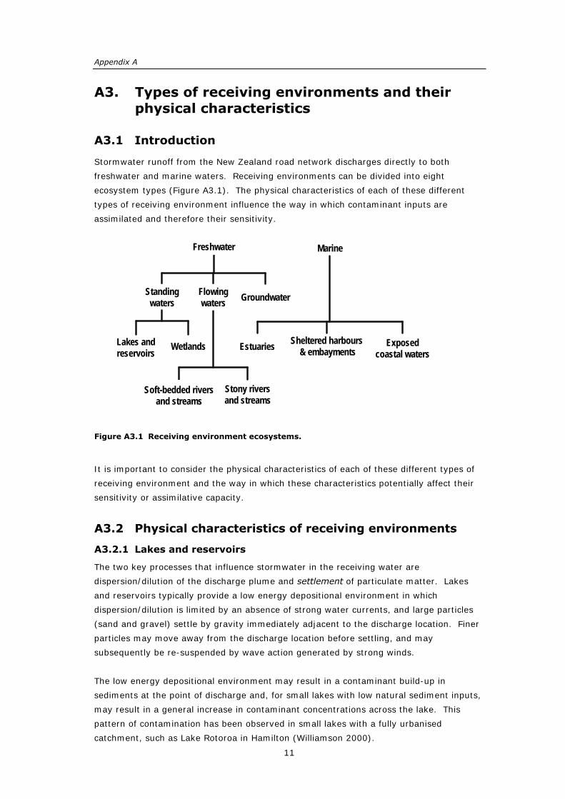
Stormwater runoff from the New Zealand road network discharges directly to both
freshwater and marine waters. Receiving environments can be divided into eight
ecosystem types (Figure A3.1). The physical characteristics of each of these different
types of receiving environment influence the way in which contaminant inputs are
assimilated and therefore their sensitivity.
Figure A3.1 Receiving environment ecosystems.
It is important to consider the physical characteristics of each of these different types of
receiving environment and the way in which these characteristics potentially affect their
sensitivity or assimilative capacity.
A3.2 Physical characteristics of receiving environments
A3.2.1 Lakes and reservoirs
The two key processes that influence stormwater in the receiving water are
dispersion/dilution of the discharge plume and settlement of particulate matter. Lakes
and reservoirs typically provide a low energy depositional environment in which
dispersion/dilution is limited by an absence of strong water currents, and large particles
(sand and gravel) settle by gravity immediately adjacent to the discharge location. Finer
particles may move away from the discharge location before settling, and may
subsequently be re-suspended by wave action generated by strong winds.
The low energy depositional environment may result in a contaminant build-up in
sediments at the point of discharge and, for small lakes with low natural sediment inputs,
may result in a general increase in contaminant concentrations across the lake. This
pattern of contamination has been observed in small lakes with a fully urbanised
catchment, such as Lake Rotoroa in Hamilton (Williamson 2000).
WetlandsLakes andreservoirs
Stony riversand streams
Soft-bedded riversand streams
GroundwaterStandingwaters
Flowingwaters
Freshwater
Exposedcoastal waters
Estuaries Sheltered harbours & embayments
Marine

IDENTIFYING SENSITIVE RECEIVING ENVIRONMENTS AT RISK FROM ROAD RUNOFF
12
To the extent that they form depositional environments, lakes and reservoirs are
moderately to highly vulnerable to adverse effects derived from stormwater runoff.
A3.2.2 Wetlands
A definition of wetland for New Zealand purposes is provided in the Resource
Management Act (1991):
“Wetland” includes permanently or intermittently wet areas, shallow water, and
land water margins that support a natural ecosystem of plants and animals that are
adapted to wet conditions.
The major difference between lakes and wetlands, from a scientific perspective, is depth.
Wetlands are shallow water bodies, often with light penetration to the bed, while lakes are
far deeper, resulting in the presence of both euphotic and profundal zones. These
differences in depth and light penetration may result in the presence of aquatic
macrophytes across the entire bed of a wetland while macrophyte communities in lakes
are usually restricted to the shallow littoral regions.
Like lakes and reservoirs, wetlands provide a low energy depositional environment in
which sediments and associated contaminants tend to accumulate. Indeed, the biofilms
covering aquatic plants and other surfaces in wetlands can be particularly effective at
trapping fine particulate matter from urban stormwater. This is one of the reasons that
constructed wetlands or macrophyte ponds are commonly used to provide the final
‘polish’ in stormwater and wastewater treatment processes (Timperley et al. 2001).
Wetlands are dynamic systems with water levels that may change throughout the year
from completely dry to flooded, and with plant and animal communities changing in
response. This dynamic nature, and the wide variety of wetland types (bog, fen, marsh,
saltmarsh, etc), makes it difficult to predict the way in which contaminant inputs will be
assimilated and the degree of risk they will present.
In general, it appears that wetlands are moderately to highly vulnerable to adverse
effects derived from road runoff.
A3.2.3 Soft-bedded rivers and streams
Soft-bedded rivers and streams in New Zealand are typically low relief watercourses with
relatively low water velocities, which at most times generate insufficient energy to
transport away all of the sediment inputs arriving from the catchment. This results in a
gradual build-up of bed sediments that, over time, may be balanced by occasional flood
flows which restore the base bed level by transporting accumulated sediments and
contaminants downstream.
Depending on the ratio of stormwater sediment to uncontaminated sediment, elements
such as zinc may accumulate in settlement zones and potentially exert an adverse effect
on benthic organisms (e.g. Timperley 2000).

Appendix A
13
Many urban streams do not receive their normal supply of sediments and are dominated
by contaminated sediment inputs derived from roadways and other urban sources.
Furthermore, in many urban environments, stormwater flow could make up all of the flow
in the water body resulting in minimal dilution and potentially high (but transient)
concentrations of contaminants in the water column.
Timperley (2000) identified two pathways for adverse effects on aquatic life from
chemical contamination. One is the direct interaction of free, dissolved contaminants,
such as the zinc or copper ion, with animals’ gills. This can occur in the water column and
in sediment interstitial waters. The other pathway is through the incidental ingestion of
contaminated particles, usually because these are mixed with normal food particles. A
portion of the contaminants attached to particles is converted to dissolved forms in the
animals’ digestive system.
Soft-bedded streams are moderately to highly vulnerable to adverse effects derived from
road runoff due to their tendency to trap and accumulate contaminants and, in the case
of smaller urban streams, the limited capacity to dilute contaminated stormwater inflows.
A3.2.4 Stony rivers and streams
Stony-bedded rivers and streams are those higher gradient watercourses that generate
sufficient energy to transport sediments downstream. The hydraulic processes are
predominantly dispersive rather than depositional. Nevertheless, as described above for
soft-bedded streams, adverse effects on aquatic life may occur either by direct interaction
of dissolved contaminants with animals gills, or through the incidental ingestion of
contaminated particles which may be trapped on biofilms, which are grazed by some
macro-invertebrates.
In a study of urban streams in Auckland, Hamilton and Christchurch, Timperley (2000)
found that zinc was the most significant dissolved metal, with chronic (base flow) levels
possibly affecting up to 15% of aquatic organisms that could inhabit urban streams. This
study indicated that transient peak concentrations, which occur in the early stage of a
rainstorm, place additional stress on stream ecosystems but the magnitude of the effect
was not quantified. Concentrations of copper, lead and zinc in fine suspended particulate
matter were found to be very high at most sites, suggesting that ingestion of the
particulate matter by grazing animals would greatly increase their dietary exposure to
these metals.
The vulnerability of stony streams to adverse effects derived from road runoff would be in
the low to moderate range, depending on the size of the stream and its capacity to dilute
urban stormwater inflows.
A3.2.5 Groundwater
Stormwater discharging into a roadside drain, grass swale, rain garden or other form of
ground soakage may seep directly into the shallow groundwater. Its passage through
IDENTIFYING SENSITIVE RECEIVING ENVIRONMENTS AT RISK FROM ROAD RUNOFF
14
surface soils tends to filter out particulate material, which is retained near the surface of
the soil profile. Retention of dissolved constituents would depend on the soil matrix.
Stormwater entering the groundwater can therefore be expected to be substantially free
of particulate material but may not necessarily have reduced concentrations of dissolved
contaminants.
Groundwater would not normally be considered to be vulnerable to adverse effects
derived from stormwater discharges.
A3.2.6 Estuaries
Contaminants primarily adsorb to fine particulate matter in stormwater discharges
(Williamson, 1993; Leersnyder, 1993). Upon arrival at the estuary, the coarser particles
settle by gravity because of the large drop in water velocity. Finer particles are
flocculated and the resultant larger particles settle to the bed. Therefore the immediate
fate of a large proportion of the contaminants, after entering the estuary, is deposition by
settling in the upper reaches of the estuary.
Some particle and dissolved contaminants will be carried through the estuary, particularly
during large storms, and especially during low tide when storm flows are carried right
down the estuary in central incised channels. Dissolved contaminants in stormwater tend
to adsorb to particles in the estuary (ARC 2004).
Recent monitoring of sediment quality in Auckland’s urbanised estuaries by the Auckland
Regional Council shows that at some 29% of estuarine sampling sites, zinc exceeds the
initial threshold of Environmental Response Criteria (ERC) set in the Proposed Regional
Plan. Levels of copper, lead and PAH also exceed the initial threshold level at a number of
locations. The highest contaminant levels were found in settling zones of catchments with
the longest history of urbanisation.
Not surprisingly, most settling zones and outer zones away from the main urban areas,
that have catchments predominantly in rural land use, have low concentrations of these
contaminants (ARC 2004, Diffuse Sources 2004). Trend analysis of the ARC Long Term
Baseline monitoring programme demonstrates that zinc and copper concentrations are
clearly increasing at many sites, while lead concentrations are decreasing2. Stratigraphic
information from cores taken in urban estuaries confirms the increase in copper, lead and
zinc with change in land use from rural to urban. It also confirms the more recent
decrease in lead (ARC 1994, Swales et al 2002, Williamson et al 2003).
As is the case for freshwater systems, aquatic life in estuaries can be affected by
stormwater contaminants via two potential pathways. One is the direct interaction of
dissolved contaminants with animals’ gills, either in the water column or in sediment
2 Decreasing concentrations of lead are thought to reflect the removal of lead from petrol in the early 1990s.

Appendix A
15
interstitial waters. The other pathway is through the incidental ingestion of contaminated
particles mixed with normal food items.
Estuaries, particularly those within sheltered harbours, are highly vulnerable to adverse
effects derived from stormwater discharges.
A3.2.7 Sheltered harbours and embayments
Stormwater discharging to a sheltered harbour or embayment is subject to many of the
processes described above for estuaries. Several studies have recorded the build-up of
contaminants in sheltered inner harbours and some have identified adverse effects on
benthic ecology.
For example MWH (2003) records a build-up of contaminants (mainly zinc and copper)
and decreased species diversity and dominance of optimistic species in the vicinity of
stormwater outfalls in inner Wellington Harbour.
Sheltered harbours and embayments, being deposition environments, are highly
vulnerable to adverse effects derived from stormwater discharges.
A3.2.8 Exposed coastal waters
Exposed coastal waters are high-energy ecosystems in which the discharge plume and
associated particulate material is rapidly dispersed by turbulence and currents driven by
wind, wave, and tidal action as well as larger-scale influences such as ocean currents.
Contaminants derived from road runoff therefore tend to be rapidly diluted and dispersed
through coastal waters rather than accumulating around the outfall. Exposed coastal
waters have a relatively low vulnerability to adverse effects from stormwater discharges.
A4 Methods for classifying receiving environments
A4.1 Introduction
Methods for classifying receiving environments in New Zealand can be divided into two
categories:
i) Those aimed at broad classification of ecosystems, or parts of ecosystems, on the
basis of their physical or biological characteristics (‘eco-types’).
ii) Those involving attempts to classifying receiving environments according to the
characteristics considered to relate more directly to their ‘sensitivity’, and hence
their ability to assimilate contaminants without showing significant adverse
effects.

IDENTIFYING SENSITIVE RECEIVING ENVIRONMENTS AT RISK FROM ROAD RUNOFF
16
A4.2 Eco-typing approaches to classification
Eco-typing involves the grouping of ecosystems or parts of them with similar physical and
biological characteristics, the presumption being that water bodies with similar
characteristics lend themselves to similar management treatments. This being the case,
it is implicit that water bodies grouped into a specific “eco-type” have a similar degree of
sensitivity to pollution.
A4.2.1 ANZECC (2000)
A review of ecosystem classification schemes in the ANZECC water quality guidelines
(ANZECC 2000) found that three broad categories have emerged:
• Those based entirely on geography (e.g. inland, estuarine, coastal/marine).
• Those based on climate (e.g. tropical, temperate, arid).
• Those based on geography and/or climate coupled with a consideration of key
physical and biological factors.
The majority of the older classification systems (e.g., Hughes & Larsen 1988; Biggs et al.
1990) are based on physical geography and use manual classification techniques to draw
visible ecological boundaries onto maps. More recent classifications are numerically-
based using computer programs to sort climate, landform and soils data to group areas
containing ecosystems of similar type.
The ANZECC (2000) water quality guidelines classify ecosystems into six broad groups
(estuarine, coastal marine, lakes and reservoirs, wetlands, upland rivers & stream and
lowland rivers & streams), and recognises three ‘ecosystem conditions’ based on their
degree of modification. The three ecosystem conditions are:
i) High conservation/ecological value systems: Effectively unmodified or other
highly valued ecosystems, typically (but not always) occurring in national parks,
conservation reserves or in remote and inaccessible locations. The ecological
integrity is regarded as intact.
ii) Slightly-to-moderately disturbed systems: Ecosystems in which aquatic biological
diversity may have been adversely affected to a relatively small but measurable
degree by human activity. The biological communities remain in a healthy
condition and ecological integrity is largely retained. Slightly-to-moderately
disturbed systems could include rural streams receiving runoff from farmland, or
marine ecosystems lying immediately adjacent to metropolitan areas.
iii) Highly disturbed systems: These are measurably degraded ecosystems of lower
ecological value. Examples of highly disturbed systems would be some shipping
ports and sections of harbours serving coastal cities, urban streams receiving
road and stormwater runoff, or rural streams receiving runoff from intensive
horticulture.
Appendix A
17
The third ecosystem condition recognises that degraded aquatic ecosystems still retain, or
after rehabilitation may have, ecological conservation values, but for practical reasons it
may not be feasible to return them to a slightly-to-moderately disturbed condition.
ANZECC (2000) recommends that these levels of ecosystem condition be used as a
framework to decide upon an appropriate level of protection. Key stakeholders in a
region would normally be expected to decide upon an appropriate level of protection
through determination of management goals and based on the community’s long term
desires for the ecosystem.
The philosophy behind selecting a level of protection, inherent in the water quality
guidelines, is either (i) maintain the existing ecosystem condition, or (ii) enhance a
modified ecosystem by targeting the most appropriate condition level.
A4.2.2 NZWERF (2002)
The New Zealand Water and Environment Research Federation (NZWERF), in The New
Zealand Municipal Wastewater Monitoring Guidelines 2002, adopts a risk-based approach
as a basis for developing receiving environment monitoring programmes. The approach,
which is said to build on the ANZECC ecosystem classification (above), aims to ensure
that a monitoring programme devised for any given situation, amongst other things,
reflects the true risks faced by the receiving environment.
The process used in the Guidelines for the risk-based development of a monitoring
programme is termed the HIAMP process (Hazard Identification, Analysis and Monitoring
Plan). The first step of the HIAMP process involves characterisation of the discharge, the
receiving environment and community values. In Step 2 this information is fed into the
Risk Analysis (identification of ‘hazards’ associated with the discharge and/or the
receiving environment, and assessment of the potential level of impact associated with
each hazard) and hence the design of an appropriate monitoring plan in Step 3.
Classification of the receiving environment is thus a fundamental step in the HIAMP
process. As NZWERF (2002) notes, at p49:
Receiving environment classification can take many forms and can be very
complex or very general, depending on the desired outcome. For example,
physical factors such as climate, geography and biology are often used to
‘ecotype’ on environment, but social and cultural factors are also important
and might be incorporated under certain circumstances. In general,
characterisation of the receiving environment allows for the creation of
groups or types of environments, which will react in a different fashion when
exposed to a wastewater discharge.
Under the NZWERF approach, receiving environment characteristics are divided into two
primary categories: (i) type of environment (e.g. lake or estuary) and (ii) characteristics

IDENTIFYING SENSITIVE RECEIVING ENVIRONMENTS AT RISK FROM ROAD RUNOFF
18
within each environment that affect the extent to which wastewater components will be
assimilated (called ‘assimilative capacity’).
The types of receiving environment recognised by NZWERF are:
i. Lake/Reservoir
ii. River/Stream (where wastewater input is <50% base flow)
iii. River/Stream (where wastewater input is >50% base flow)
iv. Estuary
v. Harbours and sheltered embayments
vi. Nearshore marine (shoreline)
vii. Offshore marine
viii. Groundwater
The assimilative capacity characteristics of the receiving environment recognised by
NZWERF are:
i. Dilution
ii. Substrate
iii. Enrichment status
iv. Sensitivity of ecological values
v. Significant other inputs to the environment
vi. Aesthetics
vii. Human health and safety (via contact recreation)
viii. Water supply (whether or not)
ix. Food gathering
x. Cultural or spiritual value
NZWERF then applies a rather complex matrix approach to assessing, for a given
receiving environment, the hazards represented by the characteristics of the effluent and
the receiving environment characteristics, and this information is then fed into the HIAMP
model.
A4.2.3 Ministry for the Environment research
Over the last five years, New Zealand’s Ministry for the Environment has led a series of
major research projects aimed at developing a numerically-based approach to
environmental classification.
The outcome of this work includes the formulation of the ‘New Zealand River Environment
Classification’ as described by Snelder et al. (2004) and the ‘New Zealand Marine
Environment Classification’ as described by Snelder et al. (2005).
The New Zealand River Environment Classification (REC) is a spatial framework for
regional scale environmental monitoring and reporting, environmental assessment and
management. It is intended to assist with:

Appendix A
19
• organising empirical data,
• extrapolating data and information to locations with no data,
• stratifying variation in rivers so that monitoring sites can be selected and
management activities can be prioritised, and
• summarising the characteristics of types of rivers so that management
expectations and controls can be set that are justifiable and achievable.
The REC groups and classifies rivers (or parts of rivers) at six hierarchical levels, each
corresponding to a controlling environmental factor. The factors, in order from largest
spatial scale to smallest, are:
• climate,
• source-of-flow,
• geology,
• land cover,
• network position,
• valley landform.
The REC is provided as a GIS layer that can be displayed as a series of maps showing
classes at each level of the REC hierarchy.
The ‘New Zealand Marine Environment Classification’ (MEC) covers both New Zealand’s
Exclusive Economic Zone and, at a higher level of resolution, the Hauraki Gulf region.
The purpose of the classification is to provide spatial frameworks for structured and
systematic management by subdividing the geographic domain into units having similar
environmental and biological character.
The MEC may be utilised in a variety of applications including:
• Defining management units that will be subject to similar objectives, policies and
methods,
• Transferring knowledge of processes and values to other areas on the basis of
similarity,
• Predicting the potential impacts of events and resource uses based on ecosystem
susceptibility,
• Identifying priorities for protection (e.g. which parts of the environment should be
included in marine protected areas), and
• Structuring monitoring programmes to ensure they represent all environmental
types, and providing a context for reporting state of the environment information.
Both the REC and MEC classification systems provide managers with a useful framework
for broad scale environmental and conservation management. However the full utility,
and indeed limitations of the classifications, will only become clear as the classifications
are applied to management issues.
IDENTIFYING SENSITIVE RECEIVING ENVIRONMENTS AT RISK FROM ROAD RUNOFF
20
An obvious limitation in respect of road runoff risk assessment is that neither the REC nor
the MEC classification systems address estuaries, which are known to be particularly
vulnerable to stormwater contamination.
A4.3 Examples in New Zealand of ranking the sensitivity of receiving environments for management purposes
Methodologies for identifying and ranking sensitive receiving environments have been
developed in New Zealand by local and regional authorities for a variety of purposes.
Examples (discussed below) relating to the discharge of stormwater include:
• Studies commissioned by the Waitakere City Council during the preparation of
their ‘Comprehensive Urban Stormwater Management Strategy and Action Plan’
(September 2000).
• The Hawke’s Bay Regional Council’s Stormwater Contaminant Planning Maps
(GHD July 2005, in draft).
A4.3.1 Waitakere City Council
The Waitakere City Council Urban Stormwater Management Strategy identified 33
stormwater management units. They form the broad geographic basis on which
stormwater is managed in Waitakere City and are mainly defined on the basis of land use
and catchment boundaries. The stormwater management units were grouped together on
the basis of:
• a sensitivity ranking of their coastal receiving environments,
• their ecological values,
• their community use.
The marine and estuarine receiving environments of the stormwater management units
are distinguished on the basis of their geographical location and tidal flushing
characteristics. The sensitivity ranking of these receiving environments were derived in
consultation with the Auckland Regional Council by adding together factors representing
an ecological value of the water body and its vulnerability to degradation.
For example, the Upper Waitemata Harbour and enclosed Whau River mouths are
depositional, low energy, environments where fine sediment settles. Because they have
slower flushing rates than the middle Waitemata Harbour, they are more vulnerable to
water and sediment quality degradation, and so receive the highest vulnerability rating of
3.
Table A4.1 shows the sensitivity ranking for Upper Waitemata Harbour is 4 + 3 = 7, and
for Whau Estuary is 2 + 3 = 5.

Appendix A
21
Table A4.1 Sensitivity ranking of receiving environments (Waitakere City Council).
Estuarine/
marine
receiving
environment
Stormwater
management
units
Ecological value
of receiving
environment (a)
Vulnerability of
receiving
environment to
degradation (b)
Sensitivity
ranking of
receiving
environment (c)
Upper
Waitamata
Harbour
(27) Whenuapai
(25) Herald Island
(26) Redhills
4 3 7
Whau Estuary
(5) Wairau Creek
(4) New Lynn East
(3) Rewarewa etc.
2 3 5
Notes: (a) rating from 1- 5, with 5 being the highest value; (b) rating from 1-3, with 3 being the most vulnerable;
(c) ranking from 2 to 8, with 8 being the most sensitive
The receiving environment sensitivity rankings, together with a wide range of other issues
(such as community use, flooding, erosion, land development potential), were weighted
and combined into an overall prioritisation for the purpose of programming management
plans and funding of capital works. In practice, the weighting given to receiving
environment sensitivity meant that it had very little influence on the overall prioritising of
capital works.
A4.3.2 Hawke’s Bay Regional Council
The Hawke’s Bay Regional Council (HBRC) has developed a methodology for the
development of GIS information maps that classifies sensitive receiving environments and
industry types to enable more effective management of industrial stormwater discharges,
and to minimise effects on the environment (GHD 2005).
The primary classification is based on environment types, as shown in Table A4.2.
Table A4.2 Primary classification of environment type adopted by HBRC.
Category Description Environment
Types
A
Sink environment, settling & accumulation area, low disturbance
and redistribution levels – contaminants unlikely to be dispersed
to other areas.
Estuary, lake
or pond,
wetland
B
Dynamic environment – moderate levels of disturbance and
redistribution, some settlement areas and low-medium baseflow
volume with less dilution potential.
Stream
C
Dynamic environment – moderate to high levels of disturbance
and redistribution, limited settlement areas, high base flow
volume with good dilution potential.
River
D Dynamic environment – high levels of disturbance – contaminants
likely to be dispersed within 24 hours. Coast

IDENTIFYING SENSITIVE RECEIVING ENVIRONMENTS AT RISK FROM ROAD RUNOFF
22
The secondary classification (Table A4.3) takes into account the ecological value of the
environment. The tertiary classification (Table A4.4) takes account of the ability of the
environment to assimilate contaminants without major degradation.
Each area is to be classified according to the primary and secondary categories, and
possibly the tertiary classification. The primary classification is presented as a coloured
polygon on a GIS map, with the secondary and tertiary classification represented as a
number allocated to the coloured shape.
Table A4.3 Secondary classification of environment type adopted by HBRC.
Category Description
1 Classified by HBRC or DOC as important ecological areas (e.g. protected natural
area, wildlife refuge, reserve, restoration site, etc).
2 Rare or keystone species or rare habitat thought to be present (not necessarily
formally classified) or is a good representative example for the region.
3 Highly productive habitat, supports high biodiversity, acts as nursery habitat, or
provides connection between important areas.
4 Site adds to the general regional ecology.
5 Site would benefit greatly from minor-moderate restoration works.
Table A4.4 Tertiary classification of environment type adopted by HBRC.
Category Description
i
Considered already highly degraded and has minimal remaining assimilation
capacity – significant cumulative affects – contaminants may begin ‘overflowing’ to
environments.
ii Considered already moderately degraded and has a limited assimilation capacity –
cumulative effects occurring and expected to worsen.
iii Considered to be degraded and has a diminished assimilation capacity, some
cumulative effects occurring.
iv Considered to have minimal degradation, has some assimilation capacity, no
obvious cumulative effects occurring.
The industries within the region are classified on the basis of their use or production of
hazardous substances, with the secondary classification based on proximity to sensitive
receiving environments. The alpha-numeric classification system is used to create
databases of geographical areas and the resultant planning maps are expected to be
similar to land use planning maps in a district plan.
The objectives of the Hawke’s Bay Regional Council initiative have a number of similarities
with objectives of this project. The methodology for ranking sensitive receiving
environments is particularly relevant and was taken into account in developing the
ranking system in this project.

Appendix A
23
A5 Determinants of receiving environment sensitivity
A5.1 Introduction
From the literature, it is apparent that receiving environment sensitivity or vulnerability to
adverse effects can be by determined by one or a combination of several factors including
physical characteristics, ecological values, and the specific human uses or values
associated with the water body in question.
This section summarises and identifies the key factors and briefly discusses how they
influence sensitivity, drawing where appropriate from the material referred to above.
A5.2 Waterbody characteristics
The important physical characteristics of a receiving environment that influence its
vulnerability to stormwater contaminants include:
• The dilution available and the rate at which mixing and dispersion occurs (governed
by the size of the receiving water body relative to stormwater inflows, and receiving
water velocity).
• The rate of sediment deposition (governed largely by the extent of water movement,
including wave action and tidal/ocean currents).
These characteristics will influence the concentration of contaminants in the water column
near the stormwater outfall and the extent to which stormwater particulates are
transported away from the discharge point.
Low energy ‘depositional’ or ‘sink’ environments, with little water movement, are at
greatest risk of build-up of contaminants in fine sediments, to levels representing a threat
to benthic organisms. The levels of dissolved contaminants in the water column are
generally low in depositional environments (where they rapidly adsorb to fine particulate
matter). However, in some small urban streams, dissolved contaminants may represent
a threat to aquatic organisms.
Generally speaking, high energy ‘dispersive’ environments with significant water and
sediment movement (e.g. rapidly flowing rivers or open coastlines) are at low risk of
adverse effects as contaminants are rapidly mixed3, diluted and dispersed. As a guide, receiving environments can therefore be grouped according to their risk from
runoff as shown in Table A5.1.
3 The rate of which mixing occurs is governed largely by the velocity of the receiving water but the degree of turbulence can also be a significant factor.

IDENTIFYING SENSITIVE RECEIVING ENVIRONMENTS AT RISK FROM ROAD RUNOFF
24
Table A5.1 Risk-based grouping of receiving environments to runoff.
Depositional environments
(high risk) (moderate risk)
Dispersive environments
(low risk)
• Enclosed harbours, ports
• Estuaries
• Low gradient, slow-flowing
streams with small base flow
• Small lakes, reservoirs
• Wetlands
• Semi-enclosed
harbours and
embayments
• Large lakes
• Moderate velocity
rivers with medium
base flow
• Open coastline
• High gradient, fast-flowing
rivers with large base flow
A5.3 Natural values present
A receiving water can be sensitive by virtue of the high natural or ecological values
present. For example, a ‘high’ degree of sensitivity might be ascribed to receiving waters
with:
• Rare, threatened or endangered species present,
• Communities with high species diversity,
• Presence of habitats or communities that are particularly sensitive to
stormwater-related effects, or
• High conservation status (e.g. a water body identified as being of national or
regional significance, or one which is within a reserve area).
A lower degree of sensitivity is indicated by receiving waters that are characterised by:
• Relative lack of biota, or
• An environment that is impoverished, homogenous or ubiquitous.
The assignment of a high priority to protecting significant ecological values is consistent
with the RMA’s emphasis on i) avoiding adverse effects on ecosystems, ii) safe-guarding
life-support systems, iii) protecting significant indigenous vegetation and habitats of
indigenous fauna, and iv) sustaining the potential of natural resources to meet the
reasonably foreseeable needs of future generations.
At face value, it would see reasonable to afford a higher status to the ecological values
rather than the human uses values associated with a given waterbody in any system for
classifying the sensitivity of receiving environments. The reason for this is that humans
are fundamentally dependant upon the `health’ of the biosphere and ecological processes
for their long term social and economic wellbeing. This aspect is given further
consideration in Appendix C.
A5.4 Human uses and values
A receiving water may be sensitive by virtue of the human uses or values associated with
it. For example, a ‘high’ degree of sensitivity might be ascribed to receiving waters:

Appendix A
25
• Used extensively for contact recreation,
• Of high aesthetic/recreational/tourism value,
• Of cultural value e.g. valued by Maori as a customary source of food, or for
spiritual reasons, or
• Used as a drinking water source.
The objective of protecting significant human uses and values associated with water
bodies is consistent with RMA requirements to i) avoid, remedy or mitigate adverse
effects on the environment, ii) to recognise and provide for the relationship of Maori and
their culture and traditions with their ancestral lands, water, waahi tapu and other
taonga, and iii) to have particular regard to the maintenance and enhancement of
amenity values and the quality of the environment.
A5.5 Existing degree of contamination or disturbance
The extent of contamination or disturbance already present in a receiving environment
can be viewed in two quite different ways:
i. The environment is already degraded and therefore not so sensitive.
ii. It is more sensitive because maintaining or increasing the contaminant load
could increase the stress on the ecosystem, increase the size of the impacted
zone, and increase the potential for adverse effects.
The authors tentatively favour the latter view on the basis that it is consistent with the
risk-based approach to assessing sensitivity and avoidance/remediation priorities, and
because it is consistent with the requirement to take into account ‘cumulative’ effects
under the RMA.
This aspect is further discussed in Section C6 of Appendix C.
A6 Conclusions and recommendations
A6.1 Conclusions
It is apparent from the literature review that receiving environment sensitivity or
vulnerability to adverse effects can be determined by one or a combination of several
factors. These include:
• The physical characteristics of the waterbody
- The size of the water body (dispersal and dilution characteristics), or
- Water movement (determines rates of mixing, dispersion rates and
sediment deposition).
• The natural/ecological values associated with the waterbody
- Rare/endangered species,
IDENTIFYING SENSITIVE RECEIVING ENVIRONMENTS AT RISK FROM ROAD RUNOFF
26
- Rare/scientifically significant communities,
- Communities with high species diversity,
- Habitats/communities particularly sensitive to stormwater-related effects,
or
- High conservation status (e.g. a waterbody of national or regional
significance, or one within a reserve area).
• Human uses and values associated with the waterbody
- Contact recreation,
- Aesthetic/recreation/tourism values,
- Cultural values, or
- Drinking water source.
• The existing degree of contamination or disturbance.
The available information indicates that water movement is a key, if not the primary
factor, in determining the sensitivity of a receiving environment to stormwater inputs.
This is because it determines whether or not sediments are deposited (rather than
dispersed) and hence whether or not the concentrations of sediment-attached
contaminants are able to accumulate to potentially harmful levels.
Assignment of a high priority to ecological criteria in assessing receiving environment
sensitivity is consistent with the requirements of the RMA (see Section A5.3). The RMA
also requires consideration to be given to human uses and values (Section A5.4).
The international literature search to date has yielded little in the way of useful intention
pertaining to the ranking or classification of receiving environment sensitivity.
The approach taken by NZWERF (Section A4.2.2) has regard to a wide range of receiving
environment ‘types’ and assimilative capacity characteristics. However the method is
developed primarily for wastewater effluents4 and it adopts a rather complex matrix
approach to assessing, for a given receiving environment, the hazards represented by the
characteristics of the effluent and receiving environment. This information is then fed into
a model. It is understood that there has been limited ‘uptake’ of the NZWERF model by
resource management practitioners, and it seems likely that this could reflect the
complexity of the approach.
Both the Waitakere City Council and Hawke’s Bay Regional Council approaches have merit
(see Section A4.4) and have been taken into account in developing the proposed
receiving environment sensitivity rating system, as described in Section C3.5 and
Appendix C.
4 Stormwater differs significantly from wastewater in that it generally has a lesser range of contaminants of potential concern, and a high proportion of the contaminants are associated with sediment particles, as outlined in section A2.
Appendix A
27
A6.2 Recommendations
On the basis of this literature review, the following considerations have been taken into
account in developing the SRE screening methodology during Stage 2 of this Project:
• The identified ‘sensitivity factors’ including the physical characteristics,
natural/ecological values and human uses and values of the waterbody.
• The possible merits of a simple visual approach to the classification and ranking of
receiving environment sensitivity – as opposed to a complex, computer based
approach.
• The primary role that water movement plays in determining whether or not a
receiving environment is ‘depositional’ or ‘dispersive’ and hence its assimilative
capacity/susceptibility to contaminant build-up in sediments.
• The important, but secondary, role that natural/ecological values play in
determining the sensitivity of receiving environments.
• The important, but tertiary, role that human uses or values play in determining
the sensitivity of a receiving environment.
• The desirability of factoring in the existing degree of contamination or
disturbance, and other contaminant sources, when assessing the sensitivity of a
receiving environment.
A7 References
ANZECC 2000: Australian and New Zealand Guidelines for Fresh and Marine Water
Quality. Australian and New Zealand Environment and Conservation Council.
ARC 1994: Urban Stormwater Quality, Pakuranga, Auckland. Auckland Regional Council
Technical Publication 49.
ARC 2004: Management & treatment of stormwater quality effects in estuarine areas.
Auckland Regional Council Technical Publication 237.
Biggs, B.J.F., Duncan, M.J., Jowett, I.G., Quinn, J.M., Hickey, C.W., Davies-Colley, R.J. &
Close, M.E. 1990. Ecological characterisation, classification and modelling of New
Zealand rivers: an introduction and synthesis. New Zealand Journal of Marine and
Freshwater Research 24:277-304.
Diffuse Sources 2004: Regional Discharges Project – Sediment Quality Data Analysis.
Auckland Regional Council, June 2004.
GHD 2005: Stormwater Contaminant Planning Maps, Phase 1: Methodology. Hawke’s Bay
Regional Council, July 2005.
IDENTIFYING SENSITIVE RECEIVING ENVIRONMENTS AT RISK FROM ROAD RUNOFF
28
Leersnyder, H. 1993. The performance of wet detention ponds for the removal of urban
stormwater contaminants in the Auckland Region. A thesis submitted to the
University of Auckland.
Moncrieff, I. & Kennedy, P. 2004. Road Transport Impacts on Aquatic Ecosystems: Issues
and Context for Policy Development. Ministry of Transport, Wellington, New Zealand.
MWH 2003. Baseline assessment of environmental effects of contaminated urban
stormwater discharges into Wellington Harbour and the South Coast. Report
prepared for Wellington City Council, Wellington, New Zealand.
NZWERF 2002. New Zealand Municipal Wastewater Monitoring Guidelines. New Zealand
Water Environment Research Foundation. Edited by David Ray (NIWA).
Snelder, T., Biggs B.J.F. and Weatherhead, M. 2004. New Zealand River Environment
Classification User Guide. Ministry for the Environment, Wellington, New Zealand.
Snelder, T et al. 2005. The New Zealand Marine Environment Classification. Ministry for
the Environment, Wellington, New Zealand.
Swales, A., Williamson, R.B., Van Dam, L. & Stroud, M. 2002. Reconstruction of Urban
Stormwater Contamination of an Estuary Using Catchment History and Sediment
Dating Profiles. Estuaries 25, 43-56.
Timperley, M.H. 2000. Contamination in our urban streams. SWAT Newsletter, Vol 1, No
2. NIWA, Auckland, New Zealand.
Timperley, M.H., Golding, L. & Webster, K. 2001. Fine Particulate Matter in Urban
Streams: Is it a Hazard to Aquatic Life? Presentation to the Second South Pacific
Stormwater Conference, Auckland, June 2001. New Zealand Water and Wastes
Association.
Timperley, M.H. 2003. Presentation to the Third South Pacific Stormwater Conference,
Auckland, May 2003. New Zealand Water and Wastes Association.
Waitakere City Council 2000. Draft Comprehensive Urban Stormwater Management
Strategy and Action Plan, September 2000.
Whittier, T.R., Hughes, R.M. and Larsen, D.P. 1988. Correspondence between ecoregions
and spatial patterns in stream ecosystems in Oregon. Canadian Journal of Fisheries
and Aquatic Sciences 45, 1264-1278.
Williamson, R.B. 1993. Urban Runoff Data Book. Water Quality Centre Publication No 20.
Williamson, R.B. 2000. Presentation to SWAT Workshop on Sustainable Aquatic Habitats
in Human Settlements, July 2000. NIWA Hamilton, New Zealand.

Appendix A
29
Williamson, R.B., Becker, K., Kelly, S., Kennedy, P., Mathieson, T. & Timperley, M. 2003.
Regional Discharges Project – The Current and Future State of Auckland’s Coastal
Receiving Environment. Presentation to the Third South Pacific Stormwater
Conference, Auckland, May 2003. New Zealand Water and Wastes Association.

IDENTIFYING SENSITIVE RECEIVING ENVIRONMENTS AT RISK FROM ROAD RUNOFF
30

Appendix B
31
Appendix B: Development of an SRE sensitivity rating system
B1. Introduction
B1.1 Purpose
Stage 2 involved developing a screening methodology for evaluating the sensitivity of
different types of receiving environments. This included a `sensitivity rating system’
based on key attributes i.e. receiving environment type, ecological value, and human use
(including cultural) value, identified under Stage 1.
An important consideration in developing the methodology is to identify the contaminants
of primary concern and to consider their chemical or physical state in the runoff (i.e.
during transport from the road surface to receiving environments). This has a bearing on
the fate of contaminants and hence the types of receiving environments most likely to be
affected by road runoff.
This report draws on the findings of both the Stage 1 report and additional literature
review in addressing these risk factors.
The proposed methodology for determining the sensitivity rating of receiving
environments to road runoff is summarised in Section 3.5 and described more fully in
Appendix C.
B1.2 CONTENT
Appendix B covers three topics:
• Nature, transport and fate of contaminants in road runoff,
• Effects of road runoff on receiving environments, and
• Conclusions on key attributes for the sensitivity rating system.
B2. The nature, transport and fate of contaminants in road runoff
B2.1 Contaminants of concern
Road runoff contains a potentially wide range of contaminants including heavy metals,
organic compounds and sediments. Readers are referred to the Ministry of Transport
research report (Kennedy 2003) for detailed information relating to the contaminants
potentially present in road runoff and for a summary of existing knowledge relating to the
concentration of contaminants in both urban stormwater and in runoff from roads and
highways.
IDENTIFYING SENSITIVE RECEIVING ENVIRONMENTS AT RISK FROM ROAD RUNOFF
32
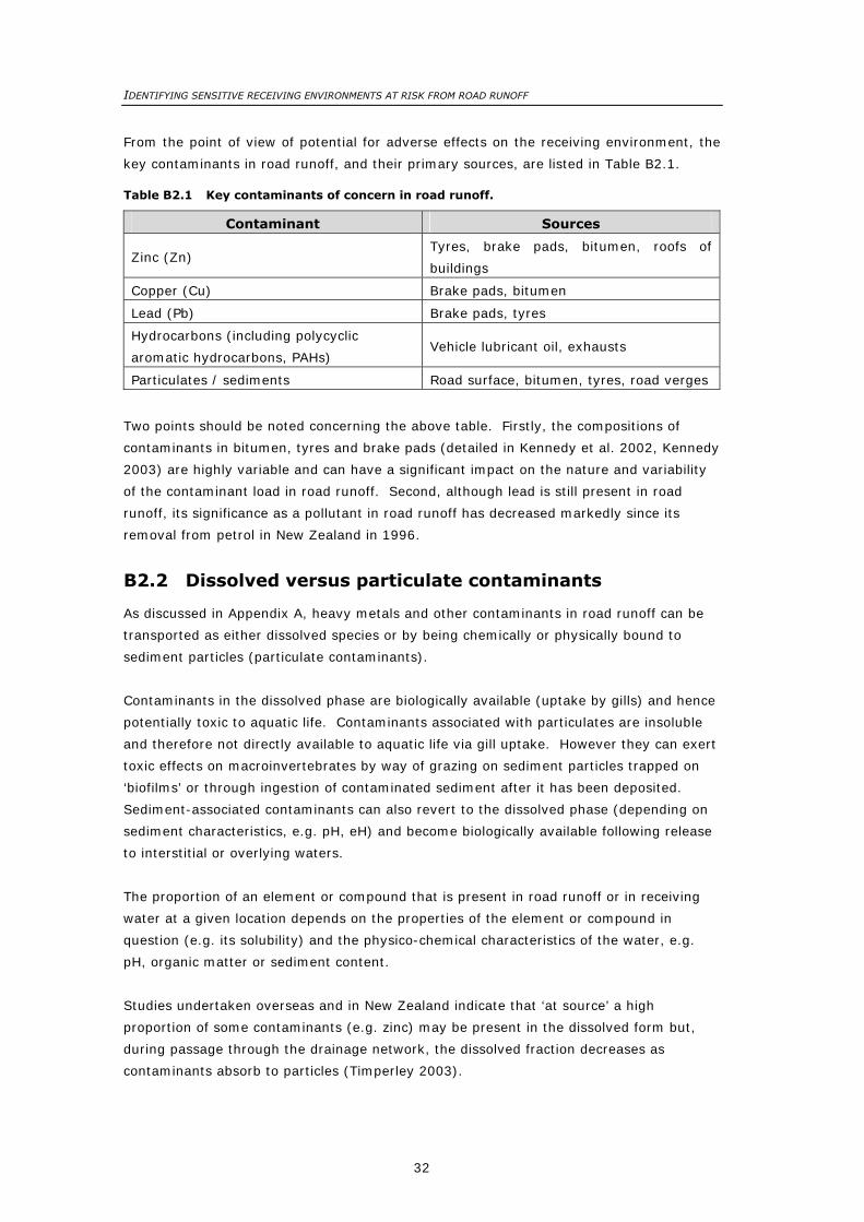
From the point of view of potential for adverse effects on the receiving environment, the
key contaminants in road runoff, and their primary sources, are listed in Table B2.1.
Table B2.1 Key contaminants of concern in road runoff.
Contaminant Sources
Zinc (Zn) Tyres, brake pads, bitumen, roofs of
buildings
Copper (Cu) Brake pads, bitumen
Lead (Pb) Brake pads, tyres
Hydrocarbons (including polycyclic
aromatic hydrocarbons, PAHs) Vehicle lubricant oil, exhausts
Particulates / sediments Road surface, bitumen, tyres, road verges
Two points should be noted concerning the above table. Firstly, the compositions of
contaminants in bitumen, tyres and brake pads (detailed in Kennedy et al. 2002, Kennedy
2003) are highly variable and can have a significant impact on the nature and variability
of the contaminant load in road runoff. Second, although lead is still present in road
runoff, its significance as a pollutant in road runoff has decreased markedly since its
removal from petrol in New Zealand in 1996.
B2.2 Dissolved versus particulate contaminants
As discussed in Appendix A, heavy metals and other contaminants in road runoff can be
transported as either dissolved species or by being chemically or physically bound to
sediment particles (particulate contaminants).
Contaminants in the dissolved phase are biologically available (uptake by gills) and hence
potentially toxic to aquatic life. Contaminants associated with particulates are insoluble
and therefore not directly available to aquatic life via gill uptake. However they can exert
toxic effects on macroinvertebrates by way of grazing on sediment particles trapped on
‘biofilms’ or through ingestion of contaminated sediment after it has been deposited.
Sediment-associated contaminants can also revert to the dissolved phase (depending on
sediment characteristics, e.g. pH, eH) and become biologically available following release
to interstitial or overlying waters.
The proportion of an element or compound that is present in road runoff or in receiving
water at a given location depends on the properties of the element or compound in
question (e.g. its solubility) and the physico-chemical characteristics of the water, e.g.
pH, organic matter or sediment content.
Studies undertaken overseas and in New Zealand indicate that ‘at source’ a high
proportion of some contaminants (e.g. zinc) may be present in the dissolved form but,
during passage through the drainage network, the dissolved fraction decreases as
contaminants absorb to particles (Timperley 2003).
Appendix B
33
The New Zealand data (e.g. Timperley 2003) indicate that zinc is the most soluble (up to
40% of total metal in the soluble phase) of the key elements in stormwater. Copper
appears to be moderately soluble (about 30%) and lead is the least soluble (<10%). A
high proportion of the total concentration of low molecular weight PAH is present in the
dissolved phase (Kennedy 2003).
The literature indicates that a high proportion of the total contaminant load arising from a
road is typically associated with the solid or particulate fraction of a discharge. Particles
are transported in suspension or in ‘bed load’ along the bottom of the stormwater pipe or
stream channel.
In the UK, (Highways Agency 2000), estimates indicate that some 60-90% of the total
copper is likely to be bound to the sediment fraction5. The solid fraction also contains
over 90% of the inorganic lead and 56% of the cadmium (Kennedy 2003).
Timperley (2001) examined the suspended solids present in urban stormwater discharges
from a variety of sources in Auckland, Hamilton and Christchurch. The results showed
that suspended material can contain high concentrations of copper (e.g. median values of
the order of 50-250 mg/kg), lead (50-400 mg/kg) and zinc (500-2500 mg/kg) with the
concentration typically increasing from residential to commercial to industrial land uses.
In estuaries it is known that most of the total copper and zinc is attached to the
particulate matter and it is thought that coagulation processes facilitate the incorporation
of these particles into sand and mudflat sediments.
PAHs, which are derived from unburnt fuel and are potentially toxic, have a higher affinity
for the sediment fraction than most other hydrocarbons (Ellis and Revitt 1991). High
molecular weight PAHs are almost entirely present in the particulate phase (Kennedy
2003).
In the UK, up to 70% of the oil deposits deposited onto a road by moving vehicles
becomes associated with the sediment fraction and may ultimately settle out on the bed
of the receiving water (Highways Agency 2000).
B2.3 The fate of contaminants in road runoff
The fate of road transport derived contaminants is primarily dependent upon the chemical
state of the contaminant (dissolved versus particulate, above) and the hydro-dynamics of
the receiving environment at the point of discharge.
5 The proportion of dissolved vs. insoluble (bound) copper in stormwater runoff and/or in a receiving environment can be influenced by the amount of dissolved organic matter (DOM) present, DOM promoting complexing of copper.

IDENTIFYING SENSITIVE RECEIVING ENVIRONMENTS AT RISK FROM ROAD RUNOFF
34
B2.3.1 Fate of dissolved contaminants
A portion of the dissolved metals and organic compounds in the runoff will be subject to
biological uptake, via animal gills, in the immediate receiving environment or in
downstream receiving environments.
However, there will be a general tendency for dissolved contaminants to be diluted and
dispersed in the receiving environment. The rate at which this occurs will vary from
situation to situation depending on the volume of the discharge and the size and mixing
characteristics of the receiving water.
Where the energy of the receiving environment is high and large volumes of water are
available for dilution (e.g. high velocity turbulent stream, or the open coast) contaminants
will disperse rapidly. There is, however, some potential for the build-up of dissolved
contaminants in the water column in low energy environments, particularly above
contaminated sediments.
B2.3.2 Fate of contaminants associated with particulate fraction
In contrast to dissolved contaminants, particulate-associated contaminants will tend to
settle and accumulate in the nearest (downstream or downcurrent) depositional receiving
environment. Solids in road runoff generally have a low particle size (predominantly
<100μ diameter) and relatively high density.
If the stormwater discharge is to a low energy section of a stream (i.e. low gradient, low
turbulence, moderately deep) then the contaminants have the potential to accumulate to
significant levels on the riverbed in the immediate receiving environment.6 In a higher
energy stream environment, contaminants will be transported downstream. In this case
there will be a tendency for them to be dispersed and therefore lower potential for build-
up to ecologically significant levels in downstream depositional areas (‘distant’ receiving
environments.)
In the case of estuarine and marine environments, there tends to be settlement of larger
particulate material immediately adjacent to the discharge point and a wider dispersion of
fine particulate matter as a result of tidal water movement or wave action. This can
result in the formation of a ‘halo’ of larger particulate material and contaminant build-up
in the sediment adjacent to inter-tidal and sub-tidal stormwater outfalls. The deposition
of contaminants in these areas is augmented by the flocculation of aggregated fine
particles at the freshwater-saltwater interface.
If the immediate receiving environment is strongly depositional (e.g. a deep, sheltered
inner harbour subject to limited water movement, a low gradient stream, or a lake) a high
proportion of the particulate load will be deposited in the immediate vicinity of the outfall.
6 Whether significant build-up of contaminant concentrations in sediments actually occurs depends in part on the natural sediment budget of the area, i.e. the extent of ‘dilution’ of contaminants by uncontaminated sediment deposited in the area.

Appendix B
35
In this event there will be high potential for the concentration of contaminants to build up
in the sediments to ecologically significant levels.
If the receiving environment is moderately depositional (e.g. rivers of moderate gradient
periodically flushed by flood-flows, or estuaries subject to moderate flushing by tide or
wave-induced currents), then contaminants have less potential to accumulate and may be
dispersed over a wider area. This can lead, for example, to contaminants discharged
from roads to the upper parts of estuaries being gradually dispersed seawards; this effect
may lower the potential for exceedance of sediment quality criteria in the medium term
but perhaps increase the potential for significant widespread contamination in the longer
term (see Auckland estuaries, Section 3.3 below).
If the immediate receiving environment is high energy/dispersive (e.g. a shallow fast-
flowing river or an open coastline), particle-associated contaminants will tend to be
rapidly dispersed and diluted. The particles will eventually settle in a distant receiving
environment but the degree of dispersion that has occurred means that there will be
limited potential for contaminant build-up in sediments.
B3 The effects of road runoff on receiving environments
B3.1 Introduction
Having considered the likely fate of the contaminants in road runoff on theoretical
grounds (chemical state and receiving environment hydro-dynamics), it is important to
consider scientific findings pertaining to the actual fate and environmental effects of road
runoff on different types of receiving environment. (The latter has assisted with
development of this methodology for the identification and ranking of sensitive receiving
environments).
There is extensive literature relating to the effects of road runoff on receiving
environments. Whilst laboratory-based testing has provided some useful information on
the toxicity of specific contaminants, it is apparent, from New Zealand and overseas field
studies, that the actual environmental effects of road runoff are site-specific. The effects
depend on the nature of the contaminant load (e.g. specific contaminants, chemical state
and total load), and a host of receiving environment variables including water movement;
available dilution and dispersal; existing water and sediment quality (e.g. contaminant
levels, pH, water hardness, dissolved organic matter content); ecological values and
human uses.
A wide-ranging review of the environmental effects of road runoff is outside the scope of
this research project. However, Kennedy (2003) has published the findings of such a
review entitled “The Effects of Road Transport on Freshwater and Marine Ecosystems”.
The report reviews both the overseas and New Zealand literature pertaining to the effects
of urban and road runoff on aquatic ecosystems.
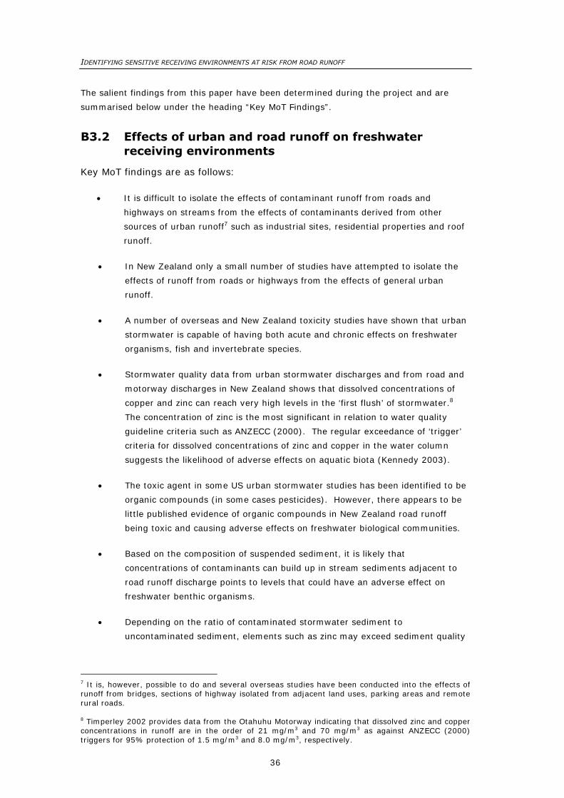
IDENTIFYING SENSITIVE RECEIVING ENVIRONMENTS AT RISK FROM ROAD RUNOFF
36
The salient findings from this paper have been determined during the project and are
summarised below under the heading “Key MoT Findings”.
B3.2 Effects of urban and road runoff on freshwater receiving environments
Key MoT findings are as follows:
• It is difficult to isolate the effects of contaminant runoff from roads and
highways on streams from the effects of contaminants derived from other
sources of urban runoff7 such as industrial sites, residential properties and roof
runoff.
• In New Zealand only a small number of studies have attempted to isolate the
effects of runoff from roads or highways from the effects of general urban
runoff.
• A number of overseas and New Zealand toxicity studies have shown that urban
stormwater is capable of having both acute and chronic effects on freshwater
organisms, fish and invertebrate species.
• Stormwater quality data from urban stormwater discharges and from road and
motorway discharges in New Zealand shows that dissolved concentrations of
copper and zinc can reach very high levels in the ‘first flush’ of stormwater.8
The concentration of zinc is the most significant in relation to water quality
guideline criteria such as ANZECC (2000). The regular exceedance of ‘trigger’
criteria for dissolved concentrations of zinc and copper in the water column
suggests the likelihood of adverse effects on aquatic biota (Kennedy 2003).
• The toxic agent in some US urban stormwater studies has been identified to be
organic compounds (in some cases pesticides). However, there appears to be
little published evidence of organic compounds in New Zealand road runoff
being toxic and causing adverse effects on freshwater biological communities.
• Based on the composition of suspended sediment, it is likely that
concentrations of contaminants can build up in stream sediments adjacent to
road runoff discharge points to levels that could have an adverse effect on
freshwater benthic organisms.
• Depending on the ratio of contaminated stormwater sediment to
uncontaminated sediment, elements such as zinc may exceed sediment quality
7 It is, however, possible to do and several overseas studies have been conducted into the effects of runoff from bridges, sections of highway isolated from adjacent land uses, parking areas and remote rural roads. 8 Timperley 2002 provides data from the Otahuhu Motorway indicating that dissolved zinc and copper concentrations in runoff are in the order of 21 mg/m3 and 70 mg/m3 as against ANZECC (2000) triggers for 95% protection of 1.5 mg/m3 and 8.0 mg/m3, respectively.

Appendix B
37
guidelines at which adverse effects could be expected to occur on benthic
organisms.9
• Contaminant concentrations in lake sediments adjacent to stormwater
discharge from roads can approach or exceed sediment quality guidelines. For
example, sediments collected adjacent to a road outfall in Hamilton Lake
revealed elevated concentrations of lead and zinc that exceeded ANZECC
guideline criteria (Rajendram 1992 in Snelder and Trueman 1995).
• Elevated concentrations of dissolved or particulate metals in road runoff have
the potential to result in bio-accumulation in freshwater biota. Elevated
concentrations of Cu, Pb, and Zn have been reported in a range of species but
there is little or no evidence of adverse effects arising from such accumulation.
• There is a wide range of organic compounds emitted by vehicles that have the
potential to bio-accumulate in aquatic organisms. The key groups are PAHs
and substituted PAHs. Although uptake of these contaminants has been shown
to occur, no adverse effects of bio-accumulation appear to have been identified.
• There is little information to indicate that any freshwater species (e.g. eel,
watercress) exposed to metals or PAHs derived from road runoff would bio-
accumulate these contaminants to a point that would result in them being
unsuitable for human consumption from a health risk perspective.
B3.3 Effects of urban and road runoff on marine receiving environments
Key MoT findings are as follows:
• As with freshwater receiving environments, it can be difficult to isolate the
effects of road runoff from the effects of contaminants from other urban
sources10.
• Most studies carried out to date in New Zealand have focused on the possible
effects of urban runoff on coastal ecosystems.
• There appears to be very few, if any, studies of the level of dissolved
contaminants in marine waters in the vicinity of stormwater discharges,
possibly because of the substantial dilution available in the sea. (Note: this is
an interpolated finding based on the lack of coverage of this issue in the MoT
reports).
• Studies in New Zealand have shown that there is a build-up of contaminants
adjacent to some urban stormwater outfall discharges to the marine environment
9 In urban areas, streams may not receive their normal supply of sediments and, as a result, sediments derived from roadways and other urbanised sources may dominate the stream. 10 Namely, when road runoff is channelled into piped or open-channel urban stormwater drainage system as is common in urban areas.

IDENTIFYING SENSITIVE RECEIVING ENVIRONMENTS AT RISK FROM ROAD RUNOFF
38
and in inter-tidal areas adjacent to roads and highways (particularly in the upper
parts of estuaries to levels approaching or exceeding ANZECC sediment quality
guidelines).
• In low energy/depositional environments, such as inner harbours and estuaries,
there is typically a ‘halo’ of sediment modification and contamination surrounding
the outfall. The size of the halo is dependent on the magnitude of the discharge,
its contaminant load and the hydrodynamic (water movement) characteristics of
the receiving environment.11 Levels of contamination adjacent to the outfall can
approach or exceed sediment quality ‘trigger’ levels, that is, levels potentially
dangerous to benthic organisms.
• In ecological terms, the most apparent effect of the discharges, within the halo, is
the replacement of normal benthic communities with an impoverished fauna of
hardy or opportunistic species. [Note – the precise nature of the cause-effect
relationship is often not clear; changes in faunal composition can potentially be
caused by changes to the physical composition of the sediments or to their
chemistry, (e.g. ammonia or sulphide build-up as a result of organic material in
runoff12), as well as by the acute or chronic toxic effects of vehicle-derived
contaminants.]
• Notwithstanding exceedence of sediment quality trigger levels, there is no direct
evidence of sediment-related toxicity nor that elevated contaminant levels are a
causal agent for changes in the benthic community.
• In the wider area of urban harbours and estuaries, sediments often contain
elevated concentrations of metal and organic contaminants as a result of
dispersion from point-source discharges (e.g. in locations such as Waitemata
Harbour it appears that all of the surface sediments are contaminated to some
degree).
• In relation to the potential for bio-accumulation, it is unlikely that road transport
contributes to any bio-uptake of contaminants by marine organisms, adjacent to
roads and urban areas.
• Current knowledge provides no information to indicate that road transport
contributes to the uptake of contaminants by marine organisms, such that they
are rendered unfit for human consumption. Two of the key trace element
contaminants – copper and zinc – are typically not bio-accumulated by many
marine organisms.13
11 The halo is normally manifested as a ‘bulls-eye’ of diminishing contaminant concentrations moving away from the outfall. The area of discernible contamination can have a diameter of 100 m or more. 12 Urban stormwater discharges typically contain a large amount of organic debris – leaves, paper, cardboard, cigarette butts, etc – from street runoff. 13 Some shellfish (e.g. oysters) can accumulate zinc.

Appendix B
39
B3.4 Summary
In summary, it is apparent that:
• There is scientific evidence that the levels of dissolved metals exceed guideline
limits for streams in the ‘first flush’ of urban stormwater runoff (and probably in
the first flush of road runoff), but no direct evidence of adverse effects on
stream organisms.
• There appears to be little evidence of build-up of road runoff–derived
contaminants in the sediments of streams to levels representing a threat to
benthic organisms, but it is likely that this does occur adjacent to some road
runoff outfalls.
• There is evidence of build-up of contaminants adjacent to outfalls in marine
depositional environments (i.e. sheltered inner harbours and estuaries) to levels
approaching or exceeding sediment quality guidelines.
• There are typically changes to the composition of benthic fauna within the
contamination ‘halo’ surrounding these marine outfalls, but direct causal
relationships have yet to be established.
The primary concern, from the scientific and road management perspectives, is that if
nothing is done to reduce road runoff contaminant inputs, contaminants could build up in
sediments to levels that have serious ecological effects.
B4 Conclusions on key attributes for the sensitivity rating system
As outlined in Section 2.2, contaminants can be transported in road runoff in either the
dissolved or the particulate phase, and it is the dissolved (soluble) phase that is capable
of exerting an immediate toxic effect on aquatic life.
In the UK, studies carried out on the polluting effects of road runoff have focused on the
dissolved fraction of contaminants and on riverine receiving environments, presumably on
the basis that there are many slow-flowing low gradient lowland streams in the UK with
limited dilution and dispersal, and coastal environments tend to have high available
dilution. Another reason for this focus could be that the UK has an extensive, heavily-
trafficked network of highways and trunk (main) roads which already have treatment
devices aimed at minimising the runoff of solids.
In the case of dissolved contaminants, the principal factors determining the sensitivity of
a receiving environment to adverse effects are the available dilution and the quality of the
receiving water. In a UK study entitled “Identification of Outfalls Posing a Pollution Risk”
(Highways Agency 2000), the primary inputs to the model that was adopted for assessing

IDENTIFYING SENSITIVE RECEIVING ENVIRONMENTS AT RISK FROM ROAD RUNOFF
40
potential impacts on receiving watercourses were low flow and upstream water quality
data.
In New Zealand, streams are generally of higher gradient, water velocity is greater, and
hence there tends to be a higher assimilative capacity for dissolved contaminants.14 This
may explain why there has been relatively little concern about the effects of the dissolved
contaminant component in road runoff in New Zealand. Although the dissolved fraction
can build up to high levels in urban streams, possibly in exceedance of ANZECC trigger
levels, in the ‘first flush’ of runoff (see Section 3.2) high levels of dissolved contaminants
do not persist in the runoff.
The main focus of concern in New Zealand (amongst resource managers and researchers)
has been the potential for build-up of contaminants in sediments adjacent to urban
stormwater outfalls and road runoff outfalls, with a particular focus on sheltered marine
receiving environments. The focus on the latter, rather than riverine receiving
environments, probably reflects a number of factors including the settlement and road
patterns in New Zealand and the dispersive nature of many New Zealand rivers and
streams.
In some urban areas, particularly Auckland, considerable management effort is being
directed to controlling inputs of particulate material into freshwater and marine receiving
environments. This approach is justifiable because, as outlined in previous sections of
this paper, the available scientific evidence indicates that:
1. A high proportion of the contaminants of concern (viz. metals, PAHs, and oils)
is strongly associated with the solids fraction in road runoff.
2. There is a tendency for dissolved contaminants to absorb to particles during
passage through the drainage system to the final receiving environment.
3. Contaminants associated with particulates demonstrably accumulate in
certain depositional environments to levels exceeding sediment quality
guidelines, e.g. in inner harbours and the upper parts of estuaries.
4. There is potential for uptake of contaminants from sediments by benthic
organisms (and food chain accumulation) by way of incidental ingestion with
food particles or by way of gill uptake of dissolved contaminants released
from sediments into interstitial waters or the waters above sediments.
5. In contrast to the situation with dissolved contaminants in rivers, benthic
organisms in sedimentary deposits can have long-term exposure to high
contaminant levels.
14 It is appreciated by the research team that this is a generalisation and does not always hold true.

Appendix B
41
6. Particulates and associated contaminants have the potential to be deposited
on ‘biofilms’ on rocks or macro-algae in rivers and in the marine environment,
and incidentally ingested by grazing macro-invertebrates.
7. Particles from urban or road runoff can have adverse ecological effects in their
own right by smothering biota or by altering the physical nature of sediments
in the vicinity of outfalls.
8. The particulate fraction of road runoff is more amenable to removal (via
source control, in-pipe and end-of-pipe treatment systems) than is the
dissolved/soluble fraction.
The above considerations suggest that the focus in this research project on the particulate
fraction of the contaminant load is appropriate and that the primary factor determining
the impact of sediment-associated contaminants is whether or not the immediate
receiving environment is depositional or dispersive. Solids will settle rapidly in still or
slow flowing water and will tend to accumulate near the outfall. In more dispersive
environments there will be limited potential for contaminants to accumulate.
This approach has guided development of the proposed methodology for ranking the
sensitivity of receiving environments to road runoff, as described in Section 3.5 and
Appendix C.
B5 References
ANZECC 2000: Australian and New Zealand Guidelines for Fresh and Marine Water
Quality. Australian and New Zealand Environment and Conservation Council.
ARC 1994: Urban Stormwater Quality, Pakuranga, Auckland. Auckland Regional Council
Technical Publication 49.
ARC 2004: Management & treatment of stormwater quality effects in estuarine areas.
Auckland Regional Council Technical Publication 237.
Biggs, B..J.F., Duncan, M.J., Jowett, I.G., Quinn, J.M., Hickey, C.W., Davies-Colley, R.J. &
Close, M.E. 1990. Ecological characterisation, classification and modelling of New
Zealand rivers: an introduction and synthesis. New Zealand Journal of Marine and
Freshwater Research 24: 277-304.
CIRIA (1994): CIRIA Report 142 Control of Pollution from Highway Drainage Discharges.
Diffuse Sources 2004: Regional Discharges Project – Sediment Quality Data Analysis.
Auckland Regional Council, Auckland, New Zealand.
Ellis, J.B. & Revitt, D.M. 1991. Incidence of heavy metals in street surface sediments:
Solubility and grain size studies. Water, Air, and Soil Pollution 17: 87-100.

IDENTIFYING SENSITIVE RECEIVING ENVIRONMENTS AT RISK FROM ROAD RUNOFF
42
GHD 2005: Stormwater Contaminant Planning Maps, Phase 1: Methodology. Hawke’s Bay
Regional Council, Hawke’s Bay, New Zealand.
Highways Agency (UK), 2000: Identification of Outfalls Posing a Pollution Risk. Report
prepared for UKHA by Thorburn Colquhoun, October 2000.
Kennedy, P., Gadd, J. & Moncrieff, I. 2002. Emission factors for contaminants released
by motor vehicles in New Zealand. Ministry of Transport, Wellington and
Infrastructure Auckland, New Zealand.
Kennedy, P. 2003. The Effects of Road Transport on Freshwater and Marine Ecosystems.
Ministry of Transport, Wellington, New Zealand.
Leersnyder, H. 1993. The performance of wet detention ponds for the removal of urban
stormwater contaminants in the Auckland Region. A thesis submitted to the
University of Auckland.
Moncrieff, I & Kennedy, P. 2004. Road Transport Impacts on Aquatic Ecosystems: Issues
and Context for Policy Development. Ministry of Transport, Wellington, New Zealand.
MWH 2003. Baseline assessment of environmental effects of contaminated urban
stormwater discharges into Wellington Harbour and the South Coast. Report
prepared for Wellington City Council, Wellington, New Zealand.
NZWERF 2002. New Zealand Municipal Wastewater Monitoring Guidelines. NZ Water
Environment Research Foundation. Edited by David Ray (NIWA).
Rajendram, G. 1992. Study of selected chemical constituents in water, sediments, plants
and fish in Lake Rotorua, Hamilton, and their possible effects on the Lake ecosystem.
Unpublished MSc thesis, University of Waikato.
Snelder, T. & Trueman, S. 1995. The environmental impacts of urban stormwater runoff.
ARC Technical Publication No. 53.
Snelder, T, Biggs B.J.F. & Weatherhead, M. 2004. New Zealand River Environment
Classification User Guide. Ministry for the Environment, Wellington, New Zealand.
Snelder, T. et al. 2005: The New Zealand Marine Environment Classification. Ministry for
the Environment, Wellington, New Zealand.
Swales, A., Williamson, R.B., Van Dam, L. & Stroud, M. 2002. Reconstruction of Urban
Stormwater Contamination of an Estuary Using Catchment History and Sediment
Dating Profiles. Estuaries 25, 43-56.

Appendix B
43
The Highways Agency, the Scottish Office Development Department, the Welsh Office, The
Department of the Environment for Northern Ireland, 1998. Water Quality and
Drainage. Design Manual for Roads and Bridges, Volume II, Section 3 (Environmental
Assessment Techniques) and Annexes I, II, III and IV.
Timperley, M 1999. Contaminant bioavailability in urban stormwater. Pp 67-74 in
Comprehensive Stormwater and Aquatic Ecosystem Management, First South Pacific
Conference, 22-26 February, 1999. Auckland, New Zealand.
Timperley, M. 2000. Contamination in our urban streams. SWAT Newsletter, Vol 1, No
2, NIWA, Auckland, New Zealand.
Timperley, M., Golding, L. and Webster K. 2001. Fine Particulate Matter in Urban
Streams: Is it a Hazard to Aquatic Life? Presentation to the Second South Pacific
Stormwater Conference, Auckland, June 2001. New Zealand Water and Wastes
Association.
Timperley, M. 2002. Urban contaminants research: Transport-Streams-Estuaries.
Roading and Stormwater Technical Workshop. 6-7 May 2002, Wellington. Workshop
jointly presented by the Road Controlling Authorities’ Forum, Ministry of Transport and
New Zealand Water & Wastes Association.
Timperley, M., Bailey, G., Pattinson, P. & Kuschel, G. 2003. Zinc copper and lead in road
runoff. 26th Australasian Transport Research Forum, Wellington, New Zealand.
Timperley, M. 2003. Presentation to the Third South Pacific Stormwater Conference,
Auckland, May 2003. NZ Water and Wastes Association.
Waitakere City Council 2000: Draft Comprehensive Urban Stormwater Management
Strategy and Action Plan, September 2000. Waitakere City Council, New Zealand.
Whittier, T.R., Hughes, R.M. & Larsen, D.P. 1988. Correspondence between ecoregions
and spatial patterns in stream ecosystems in Oregon. Canadian Journal of Fisheries
and Aquatic Sciences 45, 1264-1278.
Williamson, R.B. 1993. Urban Runoff Data Book. Water Quality Centre Publication No
20.
Williamson, R.B. 2000. Presentation to SWAT Workshop on Sustainable Aquatic Habitats
in Human Settlements, July 2000. NIWA Hamilton, New Zealand.
Williamson, R.B., Becker, K., Kelly, S., Kennedy, P., Mathieson, T. & Timperley, M. 2003.
Regional Discharges Project – The Current and Future State of Auckland’s Coastal
Receiving Environment. Presentation to the Third South Pacific Stormwater
Conference, Auckland, May 2003. New Zealand Water and Wastes Association.

IDENTIFYING SENSITIVE RECEIVING ENVIRONMENTS AT RISK FROM ROAD RUNOFF
44

Appendix C
45
Appendix C: Rating the sensitivity of receiving environments to road runoff
C1 Rating framework
A preliminary framework for the sensitivity rating system of receiving environments to
road runoff is given in Table C1.1. Receiving environments are sequentially classified
according to their:
• Physical ‘type’ (depositional versus dispersive),
• Ecological values, and
• Human uses and values (including cultural values).
A description of these three attributes is provided in the following sections.
C2 Receiving environment type classification
The receiving environment type classification is regarded as the primary classification and
weighted accordingly. This approach is based on the premise that low energy
depositional or ‘sink’ environments, with little water movement, are at greatest risk of
build-up of contaminants in sediments to levels representing a risk to aquatic organisms
or human use values.
Conversely, high energy dispersive receiving environments with significant water
movement (e.g. rapidly flowing rivers or open coastlines) are at low risk of adverse
effects as contaminants are rapidly mixed, diluted and dispersed. In short, dispersive
receiving environments have a higher assimilative capacity than depositional receiving
environments.
Receiving environments can be broadly partitioned into ‘Strongly Depositional’,
‘Moderately Depositional’ and ‘Dispersive’ reflecting their intrinsic sensitivity (see Table
C1.1).
C2.1 Strongly depositional receiving environments
Enclosed sheltered harbours and embayments and estuaries tend to be strongly
depositional and these receiving environments, when near urban areas and/or adjacent to
high density traffic roads, are the ones most commonly identified as having elevated
levels of contaminants in their sediments, particularly in the vicinity of stormwater
outfalls.
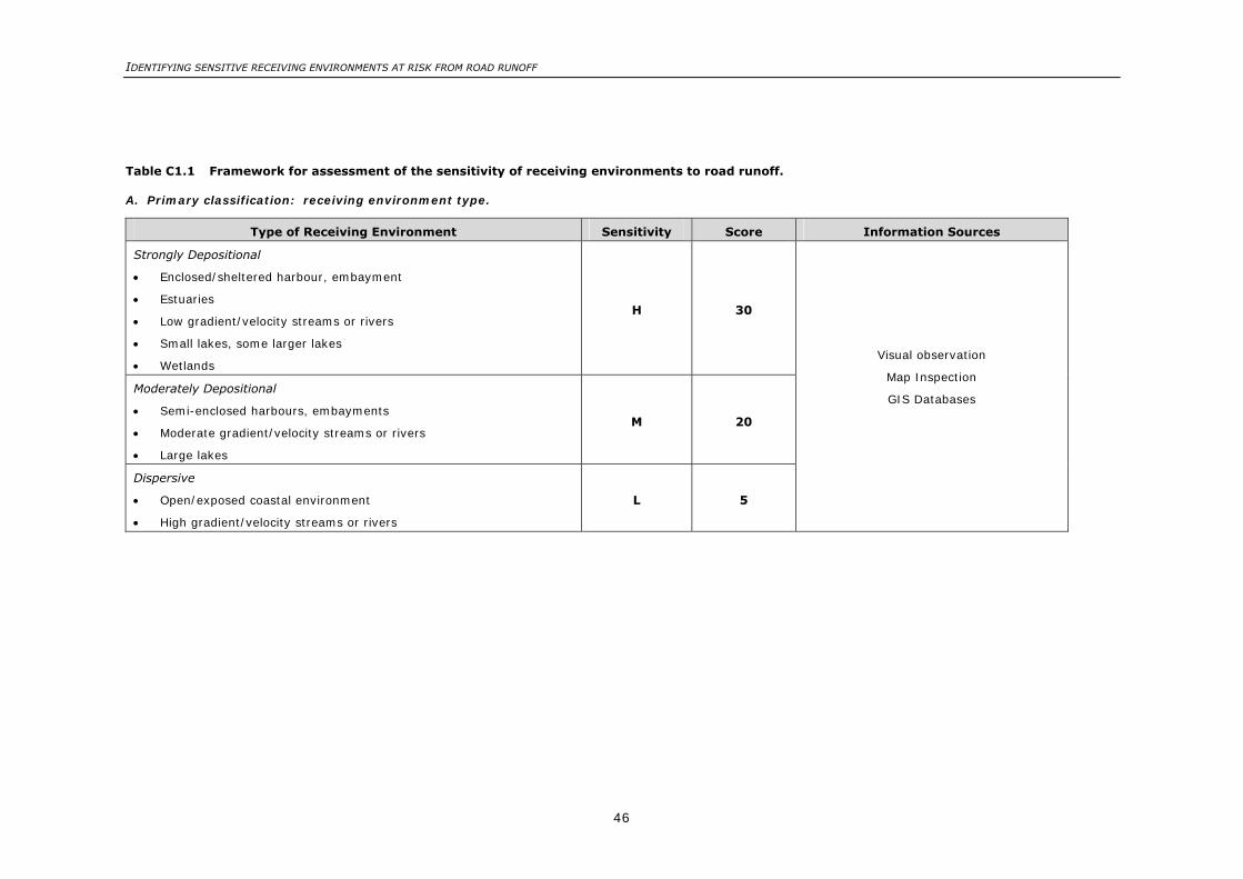
IDENTIFYING SENSITIVE RECEIVING ENVIRONMENTS AT RISK FROM ROAD RUNOFF
46
Table C1.1 Framework for assessment of the sensitivity of receiving environments to road runoff.
A. Primary classification: receiving environment type.
Type of Receiving Environment Sensitivity Score Information Sources
Strongly Depositional
• Enclosed/sheltered harbour, embayment
• Estuaries
• Low gradient/velocity streams or rivers
• Small lakes, some larger lakes
• Wetlands
H 30
Moderately Depositional
• Semi-enclosed harbours, embayments
• Moderate gradient/velocity streams or rivers
• Large lakes
M 20
Dispersive
• Open/exposed coastal environment
• High gradient/velocity streams or rivers
L 5
Visual observation
Map Inspection
GIS Databases
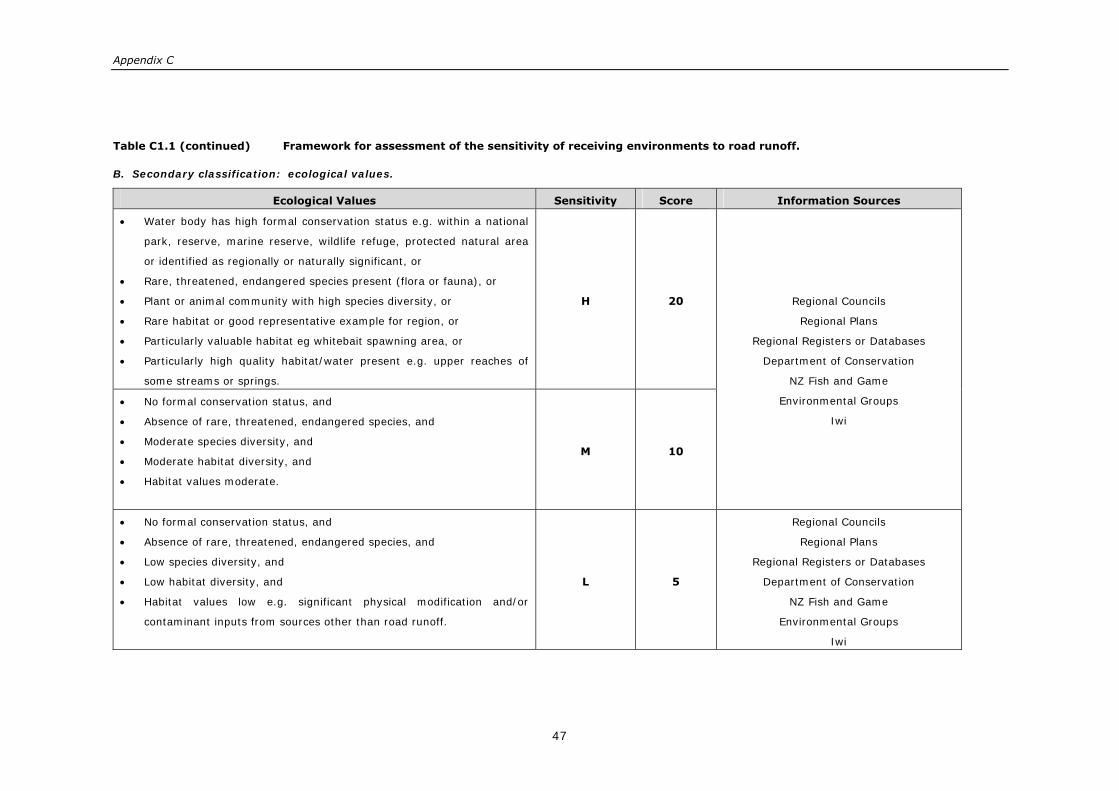
Appendix C
47
Table C1.1 (continued) Framework for assessment of the sensitivity of receiving environments to road runoff.
B. Secondary classification: ecological values.
Ecological Values Sensitivity Score Information Sources
• Water body has high formal conservation status e.g. within a national
park, reserve, marine reserve, wildlife refuge, protected natural area
or identified as regionally or naturally significant, or
• Rare, threatened, endangered species present (flora or fauna), or
• Plant or animal community with high species diversity, or
• Rare habitat or good representative example for region, or
• Particularly valuable habitat eg whitebait spawning area, or
• Particularly high quality habitat/water present e.g. upper reaches of
some streams or springs.
H 20
• No formal conservation status, and
• Absence of rare, threatened, endangered species, and
• Moderate species diversity, and
• Moderate habitat diversity, and
• Habitat values moderate.
M 10
Regional Councils
Regional Plans
Regional Registers or Databases
Department of Conservation
NZ Fish and Game
Environmental Groups
Iwi
• No formal conservation status, and
• Absence of rare, threatened, endangered species, and
• Low species diversity, and
• Low habitat diversity, and
• Habitat values low e.g. significant physical modification and/or
contaminant inputs from sources other than road runoff.
L 5
Regional Councils
Regional Plans
Regional Registers or Databases
Department of Conservation
NZ Fish and Game
Environmental Groups
Iwi

IDENTIFYING SENSITIVE RECEIVING ENVIRONMENTS AT RISK FROM ROAD RUNOFF
48
Table C1.1 (continued) Framework for assessment of the sensitivity of receiving environments to road runoff.
C. Tertiary classification: human uses and values (a)
Uses/Values Sensitivity Score Information Sources
• Highly used or valued for food gathering including traditional Maori
food sources (e.g. shellfish, koura, watercress), or
• High use for contact recreation (e.g. swimming, paddling), or
• High use for non-contact recreation (e.g. fishing, canoeing,
windsurfing, boating), or
• High cultural/spiritual values associated with water body, or
• Downstream water supply, or
• High economic value e.g. tourism.
H
10
Regional Councils
Iwi
Recreational Groups
• Highest status reasonably assigned to the receiving water, in terms of
all of the above uses or values is ‘moderate’ (see guidance in text). M 5
The status reasonably assigned to the receiving water, in terms of all of the
above uses or values, is ‘low’ (see guidance in text). L 2
TOTAL SCORE (minimum 20 and maximum 60)
Notes: Overall Sensitivity Rating: high sensitivity = total score >40
medium sensitivity = total score 20-40
low sensitivity = total score <20
(a) Some users of the methodology may wish to remove aspects concerning Maori culture/values from the weighting table (and hence from assessment of human
values) and treat this as a separate qualitative decision-making criterion

Appendix C
49
For example, trend analysis of the Auckland Regional Council’s Long Term Baseline
Monitoring Programme shows that zinc and copper concentrations in sediments in the
upper parts of Auckland’s urbanised estuaries are increasing. In strongly depositional
environments, impacts are likely to be local as there is little or no remobilisation of solids
beyond the initial point of settlement.
In the case of low gradient, moderately deep, streams and rivers (usually in the lower
parts of catchments), water velocity is low and there is potential for the contaminants
attached to fine-grained sediments to accumulate near the point of discharge. Depending
on the ratio of contaminated particles to ‘natural’ uncontaminated sediment, there is
potential for contaminant sediment to build up to levels harmful to aquatic life (see
Section B3.2, Appendix B).
In some cases, such streams or sections of streams, may be subject to periodic flushing
of the sediments by floodwaters. This is an issue that needs to be considered when
deciding whether or not a receiving environment should be classified as strongly
depositional. (If the receiving environment is so flushed, it is probably better classified as
‘moderately depositional’ reflecting the lower degree of risk.)
Lakes (more or less static water bodies with no tidal or oceanic currents) tend in general
to be strongly depositional environments due to the relative lack of water movement.
Consequently, ecologically significant ‘halos’ of sediment contamination can build up
adjacent to shoreline outfalls. However, some lakes, depending on their size and degree
of exposure to winds can have significant wave action that can help to disperse
contaminants and therefore make them less sensitive to the effects of runoff. Some
larger lakes with shallow shorelines fall into this category and may therefore be best
classified as ‘moderately depositional’. Most small lakes are best classified as ‘strongly
depositional’ due to reduced water movement and generally lower assimilative capacity.
Wetlands, which are generally static waterbodies with vegetation impeding the movement
of water, are usually appropriately classified as strongly depositional.
C2.2 Moderately depositional receiving environments
Semi-enclosed harbours and embayments, with some water movement, should be
classified as ‘moderately depositional’ even though there may be some doubt about the
extent to which contaminants are likely to accumulate in bottom sediments.
Similarly, rivers and streams of moderate gradient and water velocity should be classified
as moderately depositional. As indicated above, there may be a case for classifying some
low gradient streams as such on the basis of considerations such as water depth and
likelihood of sediment flushing during floods.
Some larger lakes may be classified as moderately depositional if there is strong wave
action and shallow water adjacent to the subject outfall.

IDENTIFYING SENSITIVE RECEIVING ENVIRONMENTS AT RISK FROM ROAD RUNOFF
50
C2.3 Dispersive receiving environments
Open, exposed, high energy coastal environments should be classified as ‘dispersive’ as
contaminants in road runoff – be they dissolved or attached to particulates – will be
rapidly dispersed away from the discharge point, particularly where the discharge is to the
intertidal area or above the wave base which is commonly the case.
High gradient, fast flowing rivers, particularly shallow rivers (or streams), are turbulent
and both dissolved and particulate-associated contaminants will be rapidly diluted and
dispersed downstream. In other words, they do not accumulate in the immediate
receiving environment.
However, fast-flowing rivers effectively act as conduits for the pollutant load that
accumulates downstream such as an estuary or harbour. While such rivers should be
classified as ‘dispersive’ receiving environments, the assessment will need to consider
impacts on the distant depositional receiving environment.
C3 Ecological values classification
The ecological values associated with a receiving environment are clearly an important
consideration. Assignment of a high priority to ecological criteria in assessing receiving
environment sensitivity is consistent with the Resource Management Act’s emphasis on
avoiding adverse effects on ecosystems, safe-guarding life support systems, protecting
significant vegetation and habitats of indigenous fauna, and sustaining the potential of
natural resources to meet the reasonably foreseeable needs of future generations.
The methodology treats ecological values as a secondary consideration relative to
receiving environment type and the scores are weighted accordingly. This is because if
the latter is dispersive there is very little risk to the receiving environment (i.e. it is
relatively ‘insensitive’), irrespective of the ecological values present.
The proposed ecological criteria (values) shown in Table C1.1 are preliminary and the way
they have been classified into groups of ‘high’, ‘medium’ and ‘low’ ecological status are
open to debate and could be reviewed in discussion with relevant agencies and interested
parties. However they are considered appropriate for use in the sensitivity rating tool
developed under this project (see Section 3.5 of main report).
Information pertaining to ecological criteria would need to be sought from relevant
agencies, including regional councils, Department of Conservation, and NZ Fish & Game.
In some cases, information is likely to be readily available from regional councils in the
form of existing registers, plans or GIS databases.

Appendix C
51
C4 Human uses and values classification
The human uses and values associated with a given receiving environment are an
important consideration.
The objective of protecting significant human uses and values associated with water
bodies is consistent with RMA requirements to avoid, remedy or mitigate adverse effects
on the environment (widely defined to include people and communities); to recognise and
provide for the relationship of Maori and their cultural traditions with their ancestral lands,
water, waahi tapu and other taonga; and to have particular regard to the maintenance of
amenity values and the quality of the environment. (Note: It is acknowledged that some
users of the methodology may wish to remove aspects concerning Maori culture/values
from the weighting table, and hence from assessment of human values, and treat this as
a separate qualitative decision-making criterion.)
Notwithstanding the above, the proposed methodology for assessing and ranking the
sensitivity of a receiving environment treats this as a tertiary consideration (reflected in
weighting of scores). The reason for this is that the RMA places emphasis on
safeguarding life support systems and protecting ecosystems (so that there are options
for future generations and because many human uses and values are fundamentally
dependent upon the maintenance of ecological values).
C5 Disturbed ecosystems
An issue that needs to be considered, in some situations, is the extent of contamination
(water quality or sediment quality) or disturbance that is already present and how this
affects the sensitivity of a receiving environment (waterbody).
As indicated in Appendix A, a disturbed ecosystems can be viewed in two quite different
ways – that the environment is already degraded and therefore not so sensitive, or that it
is more sensitive because maintaining or increasing the contaminant load could increase
the stress on the ecosystem, either pushing it over an ecological ‘break point’ or
increasing the size of the impact zone.
This issue can be relevant to the decision as to whether or not to install a runoff
treatment system, either retrospectively or when constructing a new road. It may also be
relevant during stages that might avoid SREs, such as during route selection.
In the UK study (UK Highways Agency, 2000) aimed at identifying road outfalls posing a
pollution risk, the approach taken was that lower quality receiving waters (rivers), having
been identified, were eliminated from further consideration. The rationale for this
approach was that such water bodies were considered to be relatively insensitive to road
runoff, therefore at low risk and not warranting the installation of new or additional
treatment devices to protect the receiving water.
IDENTIFYING SENSITIVE RECEIVING ENVIRONMENTS AT RISK FROM ROAD RUNOFF
52
In Australia, the Road Transport Authority procedures for selecting treatment strategies
for road runoff provide no qualification on how to rank water bodies with existing levels of
contaminants or disturbance. However, the ANZECC (2000) water quality guidelines
recognise three ecosystems ‘conditions’, viz.:
i) Effectively unmodified systems (high ecological value).
ii) Slightly-to-moderately disturbed systems: ecosystems in which aquatic biological
diversity may have been adversely affected to a relatively small but measurable
degree by human activity. The biological communities remain in a healthy
condition and ecological integrity is largely retained. These ecosystems could
include rural streams receiving runoff from farmland, or marine ecosystems lying
immediately adjacent to metropolitan areas.
iii) Highly disturbed systems: these are measurably degraded ecosystems of lower
ecological value. Examples of highly disturbed systems would be some shipping
ports and sections of harbours serving coastal cities, urban streams receiving road
and stormwater runoff, or rural streams receiving runoff from intensive horticulture.
The third ecosystem condition recognises that degraded aquatic ecosystems still retain, or
after rehabilitation may have, ecological conservation values but for practical reasons it
may not be feasible to return them to a slightly-to-moderately disturbed condition.
ANZECC (2000) recommends that these levels of ecosystem condition be used as a
framework to decide upon an appropriate level of protection. Key stakeholders in a
region would normally be expected to decide upon an appropriate level of protection
through determination of management goals based on the community’s long-term desires
for the ecosystem. This decision would consider matters such as the assimilative capacity
of the water body, the ability to ‘clean up’ existing contamination and/or reduce existing
contaminant load or other disturbances, and the ability to recover if stress levels are
reduced. The ANZECC philosophy behind selecting a level of protection, inherent in the
water quality guidelines, is either (i) maintain the existing ecosystem condition, or (ii)
enhance a modified ecosystem by targeting the most appropriate condition level.
As indicated in Section A4.3 of Appendix A, the Hawke’s Bay Regional Council’s draft
methodology for assessing the sensitivity of receiving environments identifies that the
degree of existing degradation has a bearing on the (remaining) assimilative capacity of a
receiving environment and the potential for cumulative effects. It proposes a receiving
environment classification system that takes into account the existing degree of
degradation as a tertiary consideration.
Receiving environments will often not be significantly degraded or disturbed and the
community will often not have given consideration to the issue of (realistic) management
objectives for a given water body. For this reason, the research team considers that the
issue of existing degree of contamination/disturbance is best left out of the proposed 3-
step classification of receiving environment sensitivity described above. Moreover, the

Appendix C
53
best approach to dealing with this issue is for all parties to recognise that there will be
some situations where existing or ‘baseline’ disturbance is relevant to decisions about
whether or not new or additional treatment measures to control road runoff should be
installed.
In such cases, the regional council should be asked to advise on whether or not a
(community) consensus has been reached on the appropriate degree of protection of the
receiving environment in question as per the ANZECC recommendations discussed above.
If such agreement has not been reached, an important issue will be the likely contribution
of road runoff to the total contaminant load on the receiving environment in question. If
it is low, there may be a weaker case for the installation of road runoff treatment systems
but this is a matter that should be the subject of consultation with stakeholders.
C6 Groundwater receiving environments
Stormwater discharging into a roadside drain, grass swale, rain garden or other form of
ground soakage may seep directly into the shallow groundwater. Its passage through
surface soils tends to filter out particulate material, which is retained at on near the
surface of the soil profile. Stormwater entering the groundwater can therefore be
expected to be substantially free of particulate material but may not necessarily have
reduced concentrations of dissolved contaminants. (Retention of dissolved contaminants
would depend, amongst other factors, on properties of the soil matrix).
In the UK, there is no evidence currently available to suggest that the contamination of
groundwater from routine road runoff is a serious problem (UK Highways Agency 2000).
However, the risk of road runoff contaminating groundwater resources (particularly in the
event of a spill15) is taken seriously and regulatory authorities do not accept point source
discharges to the ground in areas that are susceptible to groundwater pollution (denoted
Source Protection Zones). In the source catchment, road discharges to ground are only
permitted if the results of an investigation are favourable and if adequate precautions are
taken such as installation of oil separators (particularly relevant in the event of a spillage)
and a properly designed soakaway aimed at removing the solid phase.
In New Zealand, with lower road and traffic densities, the risks to groundwater resources
from road runoff are lower than in the UK (where no significant problems appear to exist).
Consideration of groundwater as a receiving environment has therefore been excluded
from the scope of this research project, which has a focus on the particulate fraction and
depositional environments at risk from road runoff.
This is not to say that relevant risks, such as those from verge-side chemical use or
tanker spills, should not be recognised and taken into account when considering new road
routes and treatment system issues. Some district plans identify aquifer recharge or
15 Spillage issues and risks have not been specifically considered as part of this research project but the SRE assessment methodology developed herein could be applied to consideration of spillage risks and development of response protocols.

IDENTIFYING SENSITIVE RECEIVING ENVIRONMENTS AT RISK FROM ROAD RUNOFF
54
protection zones that should, if practicable, be avoided when planning a new route. Risks
to groundwater arising from roadside herbicide and pesticide use can only be effectively
reduced through judicious application and selection of the least persistent chemicals.
C7 References
ANZECC, 2000. Australian and New Zealand Guidelines for Fresh and Marine Water
Quality. Australian and New Zealand Environment and Conservation Council.
UK Highways Agency, 2000. Identification of Outfalls Posing a Pollution Risk. Report
prepared for UKHA by Thorburn Colquhoun, October 2000.

Appendix D
55
Appendix D: Literature review of factors affecting quality of road runoff
D1 Introduction
The primary aim of the literature review was to identify the main source risk factors (i.e.
within the road environment) that contribute to or affect the quantity of contaminants in
road runoff – and therefore place downstream SREs potentially at risk. These are the
factors that influence the quality of road runoff, as measured in terms of contaminant
load, or concentration of contaminants and volume of runoff.
The main vehicle-derived contaminants of concern in road runoff are heavy metals
(notably copper and zinc) and PAH (see Section 2 of Appendix B).
The following section reviews traffic, road and rainfall factors as these relate to runoff
quality. This is followed by a discussion of different approaches for modelling pollutant
loads in road runoff, and related Ministry of Transport research. The section is concluded
with a review of screening methodology used for assessing the impact of traffic on the
aquatic environment.
D2 Factors affecting road runoff quality
The factors affecting quality of road runoff are numerous and complex with many of these
being interrelated. Contaminants on roads may have other sources apart from vehicles
e.g. contributions from outside the road environment such as zinc from roof runoff.
Furthermore, a fraction of particulate contaminants that build up on road surfaces may
subsequently be dispersed by winds before they become washed out to the road drainage
system. In urban areas, the process of street cleaning will also reduce the contaminant
load in road runoff.
The main factors affecting quality of road runoff can be grouped broadly under the
following headings:
• Traffic conditions and road characteristics,
• Rainfall and runoff patterns, and
• Road drainage infrastructure.
The first two factors are concerned with contaminant accumulation on the road surface.
The third factor affects the contaminant wash-off process. The type of road drainage
(e.g. kerb and channel, catchpit, swale) plays a key role in controlling the pollutant load
leaving a road reserve, and therefore the risk to downstream receptors.
IDENTIFYING SENSITIVE RECEIVING ENVIRONMENTS AT RISK FROM ROAD RUNOFF
56
D2.1 Effects of traffic and road characteristics
The primary risk factor to road runoff is the density of traffic as this is the main driver of
vehicle-derived contaminants. For this reason it is expected that a direct correlation
should exist between traffic levels and the quality of road runoff.
While broad relationships have been identified from field measurements between
contaminant levels in road runoff and average vehicle flows, the literature indicates that
pollution from road runoff is very variable in nature and the relationship between traffic
density and runoff quality is complex. For example, an Australian study (Drapper et al.
2000) found that traffic density and runoff quality from highways were only weakly
correlated and not sufficiently robust to propose traffic volume as the best indicator for
roads requiring runoff treatment.
More recent research has shed light on the influence of related variables such as road
characteristics (e.g. hills, bends, intersections, traffic lights etc) that can affect driving
conditions and traffic congestion and, as a result, influence vehicle emission factors under
local conditions. Thus, contaminants derived from brake pad wear (e.g. copper) or tyre
wear (e.g. zinc) will be influenced by traffic and road attributes affecting braking such as
degree of traffic congestion, presence of intersections and topography (e.g. hills/bends).
Roads with the same traffic flows but markedly different road characteristics are found to
generate very different contaminant loads in runoff. A similar effect is found for roads of
similar type but with different levels of traffic congestion (see examples in Appendix E,
Section E4.6).
Muschack (1990) found that driving patterns influence contaminant loads. Traffic lights
on a section of highway compared to one without increased the levels of pollutants. This
was attributed to an increase in braking and acceleration with a concomitant increase in
brake lining wear, tyre abrasion and leakage of oil and exhaust gas emissions.
Drapper et al. (2000) identified elevated levels of heavy metals in road runoff from exit
lanes on a bridge. The effect of rapid vehicle deceleration at the exit resulted in increased
brake and tyre wear and higher concentrations of copper and zinc, compared with sites
without an exit lane.
The effects of varying road and traffic characteristics on the emission factors of
contaminants from vehicles is discussed more fully in the New Zealand context by
Kennedy et al. (2002).
In summary, reported variations in the quality of road runoff are partially due to differing
pollutant loads, attributable to differences in traffic/road conditions. Therefore, a model
to prioritise road sources in terms of contaminant load in runoff should take the factors
influencing these differences into account.
Appendix D
57
D2.2 Rainfall and runoff patterns
Rainfall is the medium for removing pollutants that have built up on the road surface and
is therefore a key aspect affecting the concentration of contaminants in road runoff.
The relationship of rainfall to surface water quality has been extensively studied. The
relationship is complex and a function not only of the amount of rainfall but other related
variables such as the intensity and duration of rainfall during storm events, and the
number of preceding dry days.
O’Riley (2002) cites a study by Stotz (1987) which showed that the concentration of
contaminants discharged in surface runoff was not directly dependent on traffic density.
Instead it was found to vary with wind conditions, rainfall frequency and intensity, runoff
volume and the number of preceding dry days. This was confirmed by Ball et al. (1998)
who suggested that average daily traffic (ADT) is significant only on a broad scale, with
site-by-site variations related to other factors, predominantly the number of preceding
dry days. Ball concluded that the relationship between the quality of road runoff and
traffic density required further clarification.
The concept of `first flush’ is that a large fraction of the contaminant material
accumulating on an impervious road surface is flushed off into the drainage network
during the early stage of a storm. Overseas research has shown that the peak
contaminant concentrations during first flush can vary widely during an individual event
(Sansalone and Buchberger 1997) and between events (Marsalek et al. 1997). For this
reason the concentration is generally presented in terms of the event mean
concentration.
The occurrence of a first flush is mainly dependent on the long-term build up of materials
on the road surface and the magnitude of the rainfall event (Lee et al. 2002). The first
flush may also be influenced by material from previous storm events that are flushed
from road drains e.g. catchpits or stormwater pipes (Kennedy 2003).
O’Riley et al. (2002) studied a suburban roundabout carrying moderate traffic levels and
confirmed that the first flush effect occurs under New Zealand road conditions and is
similar to that reported overseas. The first flush was demonstrated for particulate-bound
metals and PAH, however the pollutant wash-off patterns for dissolved metals were
reported to be variable and inconsistent.
More recent research conducted in New Zealand to estimate the contribution of road
runoff to total stormwater loads mass loads (Timperley et al. 2003; Timperley et al. 2005)
has involved modelling contaminant accumulation and wash-off processes. These studies
have demonstrated clearer relationships between the accumulation of dissolved and
particulate metal concentrations in road runoff and individual rain events.

IDENTIFYING SENSITIVE RECEIVING ENVIRONMENTS AT RISK FROM ROAD RUNOFF
58
The significance of first flush has been used to advantage by designing stormwater
drainage systems that capture the initial runoff, and thus are able to remove the fraction
of discharge containing the highest concentrations of contaminants (Barrett et al. 1998).
Rainfall and runoff patterns are key risk factors in the quality of runoff from individual
storm events. However, in the context of this project, and as discussed in the Stage 2
report, environmental impacts from road runoff are more aligned to the cumulative build-
up of contaminants in sediments within the receiving waterbody. Over the long term,
therefore, they are relatively insensitive to whether the pollutants that build up on a road
surface are washed off in a single large storm event or a series of smaller events. In
other words, the key determinant is the total pollutant load received by the waterbody in
the longer term.
While the factors that determine the build-up of contaminants on a road surface and their
release to stormwater are complex, in the long term it may be assumed that all such
contaminants are washed off into runoff. On this basis, for a given load to the road
surface from vehicle-derived pollutants, the pollutant load discharged in runoff is
independent of rainfall intensity or quantity.
Accordingly, for the comparison and ranking of roads that may adversely affect sensitive
receiving environments, it is appropriate only to consider the relative pollutant load
corresponding to the estimated quantity of contaminant in runoff, independent of the
contaminant concentration, rainfall or runoff pattern.
D2.3 Road drainage infrastructure
Highways with kerb and channel generate higher volumes of stormwater runoff and
pollutant loads. A significant proportion of rural state highways in New Zealand do not
have kerb and channel with the result that the pollutant load entering nearby water
bodies is reduced. The benefit of using swales alongside highway verges to further
reduce downstream pollutant loads is well known.
Road drainage infrastructure is considered in more detail in Appendix E, Section E4.4 as
an integral part of the contaminant load model.
D3 Modelling road runoff pollution
D3.1 Modelling approach
Internationally, modelling of road runoff contamination can be divided into two
categories:
i) Empirical models
ii) Source- based models

Appendix D
59
Empirical models
Empirical models are based on in situ measurement of runoff at sites with well-defined
road/traffic and landuse characteristics, and derivation of an empirical relationship
between the measured variables.
A large number of models have been developed to assess the loads of contaminants
derived from stormwater runoff. The most comprehensive model in common use is the
USEPA Stormwater Management Model (SWMM) which can cover single event and
continuous simulation of urban stormwater runoff quality and quantity.
Several authors have reported on the estimation of pollutant loads from roads, highways
and urban areas (e.g. Legret & Pagotto 1999). In these cases, the loads in stormwater
runoff are estimated from the event mean concentrations (EMC) and the volume of the
event. Total loads are then estimated by summing the loads per rainfall event for the
defined catchment.
Other studies have used measurements at selected road sites to derive an empirical
relationship between pollutant load and traffic levels. This approach is exemplified in New
Zealand by the work of Timperley et al. (2003, 2005).
Empirical models provide estimates of relative contaminant loading for differing traffic
levels or landuses. This is an effective method of assessing broad scale impacts of land
use modifications and stormwater treatment options. However, contamination load rates
within these models generally ignore or otherwise do not adequately account for differing
road types or traffic volumes. For this reason an empirical approach is not appropriate in
the context of this study.
Source-based models
Source models are based on source contributions and estimates of emission factors
derived from contaminant concentrations and emission rates. For example, for zinc as a
vehicle-derived contaminant, the pollutant load to the road surface is derived from the
sum of individual sources including contributions from tyre wear, oil leakage and exhaust
emissions. Factors are included to account for the proportion of contaminant available for
washout to the drainage system.
In New Zealand, this approach was followed in the Ministry of Transport’s research
programme (see below).
D3.2 Ministry of Transport research
The Ministry of Transport (MoT) identified effects on water quality and associated aquatic
ecosystems as one of the key impact areas of road transport. MoT (1996) reported that
the contribution of road run-off to the stormwater contaminant load was uncertain but
was considered to account for 40-50% of metals in aquatic ecosystems. However, it was
IDENTIFYING SENSITIVE RECEIVING ENVIRONMENTS AT RISK FROM ROAD RUNOFF
60
acknowledged that research in New Zealand at the time was not sufficient advanced to
quantify the contribution made by road transport to any specific effects.
For this reason, the MoT initiated a research programme to examine the effects of road
transport contaminants on aquatic ecosystems. A series of research reports was prepared
between 2000 and 2005 by Kingett Mitchell Limited, in association with Fuels and Energy
Ltd, on behalf of the Ministry (see MoT 2006 for a full listing). The reports aimed to
provide an overview as to what is known about the effects of the contaminants released
by motor vehicles in a New Zealand context. Moncrieff & Kennedy (2004) provide a
summary of the background and context of this programme.
Building on the model development research for vehicle emissions to air, a programme for
developing a Vehicle Fleet Emissions Model for water (VFEM-W) was initiated. An
overview of VFEM-W is described in Moncrieff & Kennedy (2004) and a flowchart of the
process is included in Figure 8.2 of their paper. Extensive research was conducted to
characterise pollutant loads from vehicle and road interactions. The VFEM-W model was
intended ultimately to link source, pathway and ecosystem effects, on a geospatial basis,
to assist evaluating options on stormwater management.
VFEM-W was designed to provide estimates of pollutant loads from road runoff based on
derived emissions factors from five key vehicle-derived sources (brake wear, tyre wear,
oil leakage, exhaust emissions and road surface wear). The design included provision for
modifying these emission factors based on varying driving conditions and for linkage to
the New Zealand vehicle fleet profiles. The model outputs (fleet-weighted average
emission rates of individual contaminants, by vehicle type, road type and driving
condition) were to be integrated with the local traffic network model to calculate
contaminant loads for the road network.
Initial validation and calibration of the prototype VFEM-W model is described in Kennedy
& Gadd (2003). This comprised field measurements of dust from road surfaces and
gutters on roads in Waitakere City and a comparison of emission factors (mg/VKT)
derived from these field studies with emission factors assumed by the model for road and
traffic characteristics. Further details are discussed in Section D5 of this Appendix.
The contaminant emission factors that form the basis for the MoT’s VFEW-W model are
described by Kennedy et al. (2002). However, the equations relating emission factors
and road/traffic conditions to contaminant loads have not been published and output from
the MoT’s research programme did not include an operational version of the VFEM-W
model for public use.
For the purposes of this project, the extensive research published by the MoT has been
used as a basis to derive a simple vehicle contaminant load model for estimating pollutant
load in runoff.
Appendix D
61
D4 Screening criteria for traffic impact assessment on waterbodies
A number of studies have developed screening tools for impact assessment of road
networks on receiving waterbodies. These have been used, for example, to assist
identifying road networks – or sections of roads with specific outfalls - that may
potentially have an adverse effect on the receiving environment. These studies are briefly
reviewed below with a comment on their application to the current project.
D4.1 AADT as a traffic threshold screening indicator
While AADT is not in itself a robust indicator of road runoff quality, this measure of traffic
has been used overseas as a screening tool to filter out roads that are unlikely to have a
demonstrable effect on receiving environments. This section briefly reviews overseas
practice and draws conclusions for the current research project.
UK CIRIA Stage 1 assessment
The CIRIA Stage 1 assessment (CIRIA 1994) has for many years been used a preliminary
screening tool to determine whether routine road runoff poses a risk to surface waters.
For metals (specifically copper and zinc), the impact is assessed in terms of the dissolved
component and the extent to which this is diluted by the receiving water (dilution factor is
the ratio of runoff volume to the 5 percentile river flow).
A matrix relating average traffic flow (AADT) to available dilution enables a decision to be
taken on the need for further assessment of pollutant abatement using the Stage 2
method. For example, for traffic flows between 5,000-15,000 (AADT), no further risk
assessment is required where the dilution factor is 3 or greater. For the next traffic tier
(15,000 to 30,000 AADT), the threshold rises to 4 or greater.
In terms of an effects threshold for traffic levels, the UK Highway Agency guidance for
assessing the effects of road runoff (DMRB 1998) notes that several studies have
identified virtually no noticeable effects of drainage on receiving water quality at an AADT
of less than 15,000 vehicles per day (VPD). In the AADT range 15,000-30,000, only
minor impacts have been reported.
In the UK, traffic flows vary from single carriageways - carrying in the order of 10,000
VPD - to dual 4-lane motorways carrying up to 150,000 VPD. In New Zealand, typical
AADT levels on state highways are lower e.g. a median of approximately 30,000 VPD
compared with more heavily trafficked overseas highways.
Although it is difficult to generalise, traffic levels in excess of between 5000 to 10,000
AADT would be required before the generation of adverse effects from direct road runoff
on sensitive receiving environments in New Zealand (M. Timperley, pers comm.).
IDENTIFYING SENSITIVE RECEIVING ENVIRONMENTS AT RISK FROM ROAD RUNOFF
62
UK Highways Agency - risk assessment of outfalls
The UK Highways Agency (2000) described an approach to identify outfalls on main roads
and motorways that are likely to cause a level of pollution that require the fitting of new
or additional treatment measures. The project was a comparative study of the outfalls
rather than looking at the absolute pollution threat. The `high risk’ outfalls were ranked
according to the perceived risk posed to surface watercourses. The main problem areas
identified by the study occurred where the busiest and older roads (i.e. those lacking
pollution abatement in the design) crossed areas of low-flow high quality rivers.
The methodology used a filter to screen out certain roads on the basis of a combination of
low traffic volumes and less sensitive surface water. Thus, roads with current traffic flows
less than 15,000 AADT and which cross receiving waters of Class C or lower were
excluded from the study. A second filter was then applied to the residual road network to
highlight the `high risk’ outfalls. The criteria were `all roads where current traffic flows
exceed 30,000 AADT’ or `all roads where the CIRIA Stage 1 assessment would fail’ (see
above).
Application of the UK Highway Agency AADT screening method would be difficult in New
Zealand, as not all rivers have assigned environmental quality standards.
US Environmental Protection Agency practice
The US EPA (1996) acknowledged that, while the quantity of runoff generated depended
on the frequency, intensity and duration of rain in the area, the quantity of pollutants
originating from highway vehicles is not well understood. Nevertheless, research on
highway runoff quality found that significant effects only occurred from highways (major
freeways and urban arterials) with traffic volumes exceeding about 30,000 VPD. This
value was the threshold used by the US EPA to determine whether runoff required
treatment.
Implications for using AADT as a screening indicator in New Zealand
Both the CIRIA and Highway Agency screening methods are targeted at the dissolved
metal component - there is no equivalent screening method for the insoluble (suspended)
metal component. This was an issue highlighted by the UK Highway Agency’s Design
Manual (DMRB 1998) which states that “no simple method for determining the need for
control of settleable materials in road discharges is currently available”.
For this reason, these screening methods do not have direct application to the current
project which is focussed on effects of settleable particles on depositional environments
(see Appendix B “Development of an SRE sensitivity rating system” for a more detailed
rationale).
A further limitation with AADT as a screening tool is that depositional environments are
potentially affected by indirect as well as direct runoff contributions. While an AADT
threshold may be set for a road section that discharges directly to a waterbody, this will

Appendix D
63
take no account of the effects of indirect runoff that may be discharged from the same
road further up the catchment. A further difficulty with the AADT threshold concept is
that a series of road sections that discharge directly to an adjacent waterbody may each
fall below the threshold but together exert an adverse cumulative effect on the
waterbody.
D4.2 VKT as a traffic threshold screening indicator
An alternative traffic level screening indicator to AADT is total vehicle kilometres travelled
(VKT). VKT is the product of AADT and road length, hence in a defined area is a measure
of traffic density that is easy to depict spatially by GIS.
Brown and Afflum (2002) describe a GIS-based environmental modelling system using
VKT for assessing the environmental effects of road transport plans. The system (known
as TRAEMS – Transport Planning Add-on Environmental Modelling System) was developed
using MapInfo and integrates land use information in the vicinity of the modelled road
transport network.
The stormwater quality module of TRAEMS uses total VKT on roadways within a
catchment (or sub-catchment) as a surrogate measure of pollutants that may affect
waterbodies. The assumption is made that roadway emissions within a particular
catchment will largely be washed off within that catchment. The model output is the
relative pollution potential (RPP), indicative of the potential vehicle pollution load across
sub-catchments.
An example application of the model in determining potential water pollution impacts
based on road traffic growth forecasts for Gold Coast City is given in Brown et al. 2004.
The authors acknowledge that the assumptions made in the model have not yet been
validated.
The use of VKT at the sub-catchment level (and the RPP concept) appears to be a
promising screening tool for identification of potential areas of road networks where
runoff may have elevated contaminant loads that place an SRE at potential risk. It may
be of value in the current project as the first stage (Tier 1) of screening a road network to
identify potential `hot spots’ that are subject to more detailed scrutiny under Tier 2 using
a contaminant load model.
D5 Implications of findings
The literature review has considered the significance of risk factors to SREs at source i.e.
within the road network before transport of runoff along the pathway to the receiving
environment. The main findings are summarised below:

IDENTIFYING SENSITIVE RECEIVING ENVIRONMENTS AT RISK FROM ROAD RUNOFF
64
Factors affecting quality of road runoff
• The literature indicates that pollution from road runoff is very variable in nature
and has a complex relationship with runoff quality. Traffic is the main source of
road runoff pollution with the main contaminants of concern being heavy metals
(notably copper and zinc) and PAH.
• Road characteristics and driving conditions have a strong local influence on
vehicle emission rates, and hence contaminant loads. Models for estimating
vehicle-derived contaminant loads in road runoff need to factor in these
dependencies.
• For the current project, the contaminant load (mass) rather than contaminant
concentration is the key information required from the perspective of determining
the risk posed by traffic (the source component) to depositional environments.
This requirement indicates the need for incorporation of a contaminant load model
in the overall methodology for identifying SREs at risk from road runoff.
• An extensive and recent body of New Zealand research (published in 2001-2004)
has been developed under the Ministry of Transport’s programme on road
transport and its effects on aquatic ecosystems. It is intended to use this
research as the principal source of information on sources of contaminants and
related vehicle emission factors applicable to New Zealand conditions.
Models for estimating contaminant load in road runoff
• Models for estimating road runoff contaminant load use emission factors for
vehicle-derived pollutants as a function of traffic density e.g. expressed as
mg/VKT. The contaminant load is calculated by multiplying the contaminant
emission factor by the vehicle flow and the length of the road.
• Models for road runoff have been developed in New Zealand to provide estimates
of contaminants (e.g. copper, zinc and lead) expressed in terms of mg/VKT. The
models are either empirical (i.e. relationship based on field measurements of the
variables) or source-based (i.e. relationship developed from assumptions on
pollutant emission factors for different source components).
• Contamination load rates within empirical models generally ignore or otherwise do
not adequately account for differing road types or traffic characteristics that have
a defining influence on pollutant load. For this reason a source-based model is
the preferred approach in the context of this study.
• The MoT’s research programme (road transport impacts on aquatic environments
to predict vehicle-derived pollutant loads in the environment from road runoff)
included work to develop a source-based model (VFEM-W). A published study on
validation of this model in Waitakere City showed that load predictions were

Appendix D
65
weakly correlated to measured levels of copper and zinc from road surfaces. No
working model was issued from this programme and the equations relating
emission factors and road/traffic conditions to contaminant loads have not been
published.
• Derivation of a working source-based model to estimate contaminant loads on a
comparative rather than absolute basis, and based on the MoT’s extensive
published data, would be an appropriate way forward for the current project.
Screening tools
• Screening tools for impact assessment of road networks on receiving waterbodies
have been briefly reviewed. Tools developed overseas typically incorporate AADT
banding as a means to differentiate risks from roads and are generally based on
effects on water quality at the discharge point rather than the impact of pollutant
load on depositional receiving environments.
• Traffic levels measured as AADT are a poor proxy for runoff quality. A further
limitation with AADT as a screening tool for effects on depositional environments
is that it is primarily designed for direct impacts on a waterbody, and will not
include indirect contributions that may occur higher up the catchment. It also
does not take into account cumulative impacts from road sections that discharge
to the same waterbody.
• A more robust screening indicator of source risk is total VKT in the catchment that
drains to the SRE (rather than AADT on any given road section), in order to take
account of indirect contributions and the cumulative risk from the road network.
Published research indicates that VKT at the sub-catchment level is a promising
approach for identification of road networks where runoff may potentially have
elevated contaminant loads.
On the basis of the above findings, the following two-tiered approach is recommended for
identifying and characterising the risk to SREs from traffic-sourced contaminants in road
runoff:
i. A screening tool for identifying potential `hot spots’ - areas of high traffic density
that may have an adverse impact on water quality; this is to be based on total
VKT by subcatchment and to be developed for both state highways and local road
networks;
ii. A source-based model for predicting vehicle-derived contaminant loads (to include
copper, zinc and PAH) in the identified `higher risk’ road sections, based on
emission factors from the MoT’s research programme, and factoring in the effects
of varying road/traffic conditions.
The vehicle contaminant load model developed under ii) above is described in Appendix E.

IDENTIFYING SENSITIVE RECEIVING ENVIRONMENTS AT RISK FROM ROAD RUNOFF
66
D6 References
Ball, J.E., Jenks, R. & Aubourg, D. 1998. An assessment of the availability of pollutant
constituents on road surfaces. The Science of the Total Environment 209: 243-254.
Barrett, M.E., Irish, L.B., Malina, J.F. & Charbeneau, R.J. 1998. Characterisation of
highway runoff in Austin, Texas. Journal of Environmental Engineering 124: 131-
137.
Brown, L. & Affum J. K. 2002. A GIS-based environmental modelling system for
transportation planners. Computers, Environment and Urban Systems 26, 577-590.
Brown, L. Affum J. K. & Chan A. 2004. Transport Pollution Future for Gold Coast City
2000, 2011, 2021, based on the Griffith University Transport Pollution Modelling
System (TRAEMS). Urban Policy Program, Research Monograph 7, December 2004.
Griffith University.
CIRIA 1994. Report 142: Control of Pollution from Highway Drainage Discharges.
Construction Industry Research and Information Association, London, UK.
DMRB 1998. Water Quality and Drainage. Design Manual for Roads and Bridges: Volume
II, Section 3, Part 10. The Highways Agency, The Scottish Office Development
Department, The Welsh Office, The Department of the Environment for Northern
Ireland. The Stationery Office, United Kingdom.
Drapper D., Tomlinson, R. & Williams, P. 2000. Pollutant concentrations in road runoff:
Southeast Queensland case study. Journal of Environmental Engineering 126: 313-
320.
Kennedy, P. 2003. The effects of road transport on freshwater and marine ecosystems.
Ministry of Transport, Wellington, New Zealand.
Kennedy, P. & Gadd, J. 2003. Evaluation of road surface contaminant loadings in
Waitakere City for the development of the Vehicle Fleet Emission Model – Water.
Ministry of Transport, Wellington, New Zealand.
Kennedy, P., Gadd, J. & Moncrieff, I. 2002. Emission factors for contaminants released
by motor vehicles in New Zealand. Ministry of Transport, Wellington and
Infrastructure Auckland, New Zealand.
Lee, J.H., Bang, K.W., Ketchum, L.H., Choe, J. S. & Yu, N.J. 2002. First flush analysis of
urban storm runoff. The Science of the Total Environment 293: 163-175.
Legret, M. & Pagotto, C. 1999. Evaluation of pollutant loadings in the runoff waters from
a major rural highway. The Science of the Total Environment 235: 143-150.

Appendix D
67
Marsalek, J., Brownlee, B., Mayer, T., Lawal, S. & Larkin, G.A. 1997. Heavy metals and
PAHs in stormwater runoff from the Skyway Bridge in Burlington, Ontario. Water
Quality Research Journal of Canada 32: 817-827.
Ministry of Transport 1996. Environmental externalities discussion paper. Land Transport
Pricing Study. Ministry of Transport, Wellington, New Zealand.
Ministry of Transport 2006. MoT website. http://www.transport.govt.nz/business/
multimodal/environment/ stormwater.php.
Moncrieff I. & Kennedy P. 2004. Road transport impacts on aquatic ecosystems: issues
and context for policy development. Ministry of Transport, Wellington, New Zealand.
Muschack, W. 1990. Pollution of street runoff by traffic and local conditions. Science of
the Total Environment 93: 419-431.
O’Riley, A., Pandey, S., Langdon, A. & Wilkins, A. 2002. Characterisation of runoff
contaminants from New Zealand roads, & effect of rainfall events. Transfund New
Zealand Research Report No. 228. 119pp.
Sansalone, J. & Buchberger S.G. 1997. Partitioning and first flush of metals in urban
roadway stormwater. Journal of Environmental Engineering 123: 134-143.
Stotz,G. 1987. Investigations of the surface water runoff from federal highways in the
FRG. Science of the Total Environment 59: 329-337.
Timperley, M., Bailey, G., Pattinson, P., Kushel, G. 2003. Zinc, copper and lead in road
run-off. Paper presented at the 26th Australasian Transport Research Forum,
Wellington, New Zealand.
Timperley, M., Williamson, B., Mills, G., Horne, B. & Hasan, M.Q. 2005. Sources and
loads of metals in urban stormwater. NIWA Report No AKL2004-070, June 2005.
Prepared for Auckland Regional Council, Auckland, New Zealand.
UK Highways Agency, 2000. Identification of Outfalls Posing a Pollution Risk. Report
prepared for UKHA by Thorburn Colquhoun, October 2000.

IDENTIFYING SENSITIVE RECEIVING ENVIRONMENTS AT RISK FROM ROAD RUNOFF
68

APPENDIX E
69
Appendix E: Vehicle contaminant load model
E1 Introduction
Appendix E describes how the vehicle contaminant load model (VCLM) for road runoff was
derived in terms of source data, assumptions and derivation of formulae relating annual
pollutant load to traffic and road characteristics.
A full description of the developed model is given in Section E4. This includes the four
key model equations that provide an estimate of road contaminant loads for the four
contaminants of interest (particulate matter, zinc, copper and PAH).
The extensive literature review conduct by Kennedy et al. (2002) on behalf of the Ministry
of Transport (MoT) identified and described the five main sources of contaminants to road
runoff from vehicles. These are:
1) Brake wear (see Section E3.3 of this appendix)
2) Tyre wear (see Section E3.4)
3) Oil leakage (see Section E3.5)
4) Exhaust emissions (see Section E3.6)
5) Road surface wear (see Section E3.7)
Each of the above sources is described below in terms of the nature of contaminants,
emission rate, composition and derivation of equations linking emissions rate to
road/traffic characteristics.
A summary of the model equations for deriving contaminant loads in road runoff from
vehicles prior to any stormwater containment or treatment device is described in Section
E4.2. The means for how these loads may be attenuated by stormwater containment or
treatment devices and the removal efficiencies that have been built into the model for the
contaminants of interest are discussed in Section E4.4.
E2 Road deposition and retention factors
Sections E3.3 to E3.7 of this appendix describe how the model was developed to estimate
the mass load of particulate and other contaminants released by the various vehicle-
related sources.
Once generated, the pollutants are subject to a range of physical processes that are
important since they determine the amount of contaminant deposited onto the road
surface and therefore available for transport by road runoff. Moncrieff & Kennedy (2004)
provide a detailed account of the processes and pathways that determine the fate of
contaminants released from road vehicles.

IDENTIFYING SENSITIVE RECEIVING ENVIRONMENTS AT RISK FROM ROAD RUNOFF
70
These processes (e.g. wind dispersion) may reduce the amount depositing or remaining
on the road surface prior to wash off by rainfall. This, in turn, reduces the quantity of
material available for uptake in stormwater runoff. To determine the actual load available
for road runoff the output must be corrected for losses using two factors.
The first factor is the proportion of contaminants discharged from the vehicle (or by the
vehicle movement) that is deposited on the road surface. This is termed the `road
deposition factor’ and this is discussed below for each of the main contaminant sources.
The factors used have been taken from Section 9 of Kennedy et al. (2002) which contains
a full description of their magnitude and variability.
The second factor to consider is the proportion of contaminants that are retained on the
road surface after being deposited from the vehicle. This is termed the road retention
factor. For the purposes of this model, and in the absence of definitive data in the
literature, a conservative road retention factor of 1 has been adopted for all pollutants.
It is noted that there is considerable uncertainly in the values to apply for both the above
factors, as they will be seasonally dependent and site specific. However, this will not
affect use of the model in terms of a screening tool for comparative purposes to identify
priority areas in terms of contaminant load, as the same loss factors are assumed to
apply to all areas.
E3 Derivation of model equations
E3.1 Brake wear
E3.1.1 Introduction
The two principle types of vehicle brakes, disc and drum, both have components that
wear down during normal operation. The disc brake pads and the linings and shoes used
in drum brakes (collectively known as friction linings), deteriorate with the action of
braking, releasing particles onto the road surface and into the air. The emission rate for
contaminants from brake wear is derived from the brake lining wear rate and the brake
particle composition, as discussed below.
E3.1.2 Brake lining wear rate
Indicative particle emission rates from the wear of brake linings are provided by Kennedy
et al. (2002) for a range of braking intensity and vehicle type (Table E3.1). The Average
Wear Rate is derived from data given in Table 3.1 of Kennedy et al. (2002) which is a
summary of average wear rates for motor vehicles based on an extensive international
literature review of a range of vehicle types (excluding New Zealand as no local data were
available). A wide variation is found for each vehicle type and hence the average rate in
Table E3.1 is an order of magnitude indication only.
The indicative emission rates corresponding to Low, Moderate and Intense brake use were
derived by Kennedy et al. (2002) by multiplying the Average Wear Rate by factors of 0.5,
1.5 and 2, respectively. As the authors note, these factors are arbitrary but are intended

APPENDIX E
71
to provide a spread in break pad wear rates that reflects the known variations attributable
to different driving conditions.
Table E3.1 Indicative particle emission rates from brake lining wear (mg/VKT)16.
Braking Intensity Passenger Car Light Duty Vehicle Heavy Duty Vehicle
Average Wear Rate 21 30 80
Low Brake Use 10.5 15 40
Moderate Brake Use 31.5 45 120
Intense Brake Use 42 60 160
Application of these emission rates is based on the braking situation, dictated by the road
and traffic conditions (Table E3.2). Increasing brake use is a function of braking
frequency and/or the intensity of brake use. The road terrain, dominant driving condition
and level of service (e.g. interrupted or congested) will dictate if moderate or intense
braking is applied. Low brake use is assumed as the default within the model. For a road
with a mixture of conditions, the highest applicable braking rate is applied. For example a
flat, central urban road that is congested will use the emission rate corresponding to
intense brake use.
Classification of road terrain, road type and traffic condition is defined in Annex E2.
Table E3.2 Brake use as a function of road/traffic condition.
Brake use Road/traffic condition
Intense Terrain = Mountainous
or Traffic Condition = Congested
Moderate
Terrain = Hilly
or Road Type = Central Urban
or Traffic Condition = Interrupted
Low All other conditions
E3.1.3 Brake particle composition
Average estimates of friction lining composition from relatively limited New Zealand data
were presented in Kennedy et al. (2002) as a means of determining the contaminants
generated from brake wear.
As the authors note, the very large variation in both the type of friction linings and their
composition makes it difficult to derive a meaningful average concentration for
contaminants from brake lining wear. This is compounded by the fact that dust derived
from brake wear may have different composition from the parent material. For example,
Kennedy et al. (2002) cite a huge variation in copper in brake pads in New Zealand from
a sample set of 39 that varies from 29 mg/kg (10 percentile) to 116,000 mg/kg
(90 percentile). The authors recommend an interim value of 5000 ppm.
16 Kennedy et al. (2002) page 20 Table 3.7.

IDENTIFYING SENSITIVE RECEIVING ENVIRONMENTS AT RISK FROM ROAD RUNOFF
72
Table E3.3 details the indicative concentration of the key contaminants from New Zealand
brake pad data that are used in the road runoff model to derive loading estimates. As
noted above, the values are subject to large uncertainty and are considered to be order of
magnitude.
Table E3.3 Indicative concentration of contaminants in friction lining particles.
Contaminant Average concentration (mg/kg)
Zinc17 1630
Copper18 5000
Total PAH18 16
E3.1.4 Road deposition factor
International studies (e.g. Rogge et al. 1993) have shown that up to 11% of dust from
brake lining wear will be trapped in drum brake housing, while a much smaller proportion
is expected to be retained in vehicles with disc brakes.
Kennedy et al. (2002)19 note that approximately 30% of particles emitted from brake
lining wear become airborne and are subsequently lost from the road corridor. Based on
this early study, they proposed an interim road deposition factor of 0.7 to account for the
proportion of brake wear particles available for road runoff. This figure has also been
adopted in the road runoff model.
E3.1.5 Derivation of equations
The particulate emission rates (Table E3.1), assumed deposition factor and the
breakdown of vehicle kilometres travelled (VKT) by vehicle type (from the MoT’s Vehicle
Fleet Emission Model - see Annex E1) have been combined. This allows the following
equations to be derived for particulate emission rates (mg/VKT) as a function of brake
use and vehicle type for estimating contaminant loads in road runoff:
Low Brake Use (mg/VKT) = 0.7 x [11 x (1 - %HCV) + 40 x %HCV (Equation E3.1)
Moderate Brake Use (mg/VKT) = 0.7 x [33 x (1 - %HCV) + 120 x %HCV] (Equation E3.2)
Intense Brake Use (mg/VKT) = 0.7 x [45 x (1 - %HCV) + 160 x %HCV] (Equation E3.3)
Where: %HCV = Percentage Heavy Commercial Vehicles (>=3.5tonnes) in traffic flow
17 Kennedy et al. (2002) page 21 Table 3.8, based largely on Kennedy & Gadd (2003). 18 Kennedy et al. (2002) page 22 Table 3.9, based on Rogge et al. (1993). 19 Kennedy et al. (2002) page 85, based on Cha et al. (1983).

APPENDIX E
73
These equations may be combined and simplified to give:
Brake Lining Particulate (mg/VKT) = 7.7 x Bi + 20. x %HCV x Bi (Equation E3.4)
Similarly, equations can be derived for the other contaminant indicators, utilising the
indicative concentrations in Table E3.3:
Brake Lining Zinc (ng/VKT) = 12551 x Bi + 3308 x %HCV x Bi (Equation E3.5)
Brake Lining Copper (ng/VKT) = 38500 x Bi + 101500 x %HCV x Bi (Equation E3.6)
Brake Lining PAH (ng/VKT) = 123.2 x Bi + 324.8 x %HCV x Bi (Equation E3.7)
Where:
%HCV = Percentage Heavy Commercial Vehicles (>=3.5tonnes) in traffic flow
Bi = Brake intensity factor (see Table E3.4 below)
Table E3.4 Brake intensity factor.
Brake use20 Brake intensity factor, Bi
Low 1
Moderate 3
Intense 4
E3.2 Tyre wear
E3.2.1 Introduction
Frictional forces between a vehicle tyre and the road surface results in abrasive tyre wear.
This generates tyre particulate matter which, if deposited on the roadway, contributes to
the particulate and constituent contaminant loading in road runoff.
The key factors influencing tyre wear rate are the nature of the road surface and driving
conditions. Tyre brand (design and composition) is a further significant factor.
The emission rate for contaminants from tyre wear is derived from the tyre wear rate and
tyre particle composition, as discussed below.
E3.2.2 Tyre wear rate
Kennedy et al. (2002) proposed simplified tyre particulate emissions for varying vehicle
types and driving conditions. These rates were generated from industry-supplied
20 Refer to Annex E2 for brake use classifications.

IDENTIFYING SENSITIVE RECEIVING ENVIRONMENTS AT RISK FROM ROAD RUNOFF
74
estimates of wear over the tyre lifetime, assumed tyre life, number of tyres on each
vehicle and overly simplified factoring to account for different traffic conditions.
Unfortunately, despite detailing New Zealand estimates, the tyre wear rates in Kennedy et
al. (2002) were based on a foreign estimate of private car tyre life. In addition, the wear
rates per tyre for medium and heavy commercial vehicles were calculated using the
estimated lifetime of tyres for private cars (a factor of 2.5 lower than heavy trucks).
Thus, unlike the rates for other sources, the final tyre wear rates recommended within the
Kennedy et al. (2002) report have not been incorporated in this model. The basic
methodology for calculating average tyre wear from total wear and tyre lifespan has,
however, been employed.
Average tyre wear rates (in mg/VKT) for different vehicle types were calculated by
multiplying the total wear over the tyre lifetime (W in kg/tyre) by the number of tyres (N)
and dividing by the estimated life of the tyres (L in km):
Average Tyre Wear (mg/VKT) = (W x N/L) x 106 (Equation E3.8)
The resulting average wear rates by vehicle type for this calculation, together with
supporting data, are presented in Table E3.5.
Table E3.5 Average tyre wear rate by vehicle type.
Vehicle
type Size
Wear over lifetime,
W (kg/tyre)21
Estimated
tyre life,
L (km)22
Assumed
number of
tyres, N
Average
wear rate
(mg/VKT)
Cars - 1.1 47,000 4 94
LCVs - 1.8 47,000 4 153
HCVs Small 7.5(a) 119,000(a) 6 378
- Medium 7.5(a) 119,000(a) 8 504
- Large 7.5(a) 119,000(a) 12 756
(a) Reference quotes `heavy truck’ or `heavy truck tyre’ undifferentiated by size of HCV.
As set out by Kennedy et al. (2002), research has shown that tyre wear varies with a
range of factors dependent on how the tyre interacts with the road surface. These include
road surface, tyre composition, vehicle characteristics and route and style of driving. The
most significant factor, especially with respect to this road runoff model, is the `route and
style of driving’, as these determine the frequency and magnitude of acceleration.
Different styles of driving can result in wear rates that vary by a factor of six. The route
factor can result in an order of magnitude variation in tyre wear depending on whether
the road section is straight or windy. Kennedy et al. (2002) quote variations in wear
21 Kennedy et al (2002) page 31, based on New Zealand industry estimates of material loss over tyre service life. 22 Kennedy et al (2002) page 30, based on New Zealand data from Carpenter & Cenek (1999).

APPENDIX E
75
rates that vary from straight and level driving (representing 100% of tyre life) to 76% on
slightly hilly and curvy roads, to 50% on hilly and curvy roads. The higher wear results
from increased acceleration and breaking. Similarly, roads with interrupted flows (e.g.
caused by an intersection where the driver brakes before accelerating away) will result in
higher tyre wear than free flow conditions.
Since acceleration and braking are linked, the criteria used to classify tyre wear conditions
as a function of road/traffic conditions are the same as for brake use (see Table E3.6).
Annex E2 details how the road definitions are applied.
Table E3.6 Tyre wear condition as a function of road/traffic condition.
Tyre wear condition Road/traffic condition
Intense Tyre Wear Terrain = Mountainous
or Traffic Condition = Congested
Moderate Tyre Wear Terrain = Hilly
or Road Type = Central Urban
or Traffic Condition = Interrupted
Low Tyre Wear All other conditions
E3.2.3 Tyre particle composition
As with brake (friction) linings, there is a large variation in New Zealand in both the types
of tyre and their composition and hence the composition of particles derived from tyre
wear. A summary of elemental composition of a selection of 12 tyres available in New
Zealand23 covering cars, LCVs and trucks indicated levels of zinc varying from 1,190 ppm
– 18,300 ppm, and trace levels of copper in the range <1 to 3ppm. Data for PAH
concentrations in tyres were obtained from international literature.
A summary of interim tyre compositions suitable for use in estimating contaminant
emission loads was presented in Kennedy et al. (2002). Rates for the three key
contaminants are reproduced in Table E3.7.
Table E3.7 Indicative concentrations of contaminants in tyre particles.
Contaminant Concentration (mg/kg)
Zinc 24 8310
Copper25 1
Total PAH25 226
23 Kennedy et al. (2002) page 34 Table 4.8. 24 Kennedy et al. (2002) page 38 Table 4.13. 25 Kennedy et al. (2002) page 38 Table 4.14, based on Rogge et al. (1993).
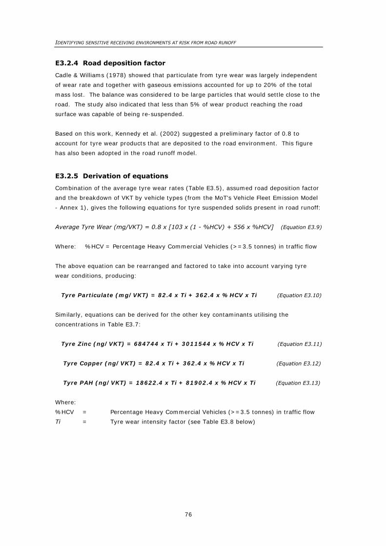
IDENTIFYING SENSITIVE RECEIVING ENVIRONMENTS AT RISK FROM ROAD RUNOFF
76
E3.2.4 Road deposition factor
Cadle & Williams (1978) showed that particulate from tyre wear was largely independent
of wear rate and together with gaseous emissions accounted for up to 20% of the total
mass lost. The balance was considered to be large particles that would settle close to the
road. The study also indicated that less than 5% of wear product reaching the road
surface was capable of being re-suspended.
Based on this work, Kennedy et al. (2002) suggested a preliminary factor of 0.8 to
account for tyre wear products that are deposited to the road environment. This figure
has also been adopted in the road runoff model.
E3.2.5 Derivation of equations
Combination of the average tyre wear rates (Table E3.5), assumed road deposition factor
and the breakdown of VKT by vehicle types (from the MoT’s Vehicle Fleet Emission Model
- Annex 1), gives the following equations for tyre suspended solids present in road runoff:
Average Tyre Wear (mg/VKT) = 0.8 x [103 x (1 - %HCV) + 556 x %HCV] (Equation E3.9)
Where: %HCV = Percentage Heavy Commercial Vehicles (>=3.5 tonnes) in traffic flow
The above equation can be rearranged and factored to take into account varying tyre
wear conditions, producing:
Tyre Particulate (mg/VKT) = 82.4 x Ti + 362.4 x %HCV x Ti (Equation E3.10)
Similarly, equations can be derived for the other key contaminants utilising the
concentrations in Table E3.7:
Tyre Zinc (ng/VKT) = 684744 x Ti + 3011544 x %HCV x Ti (Equation E3.11)
Tyre Copper (ng/VKT) = 82.4 x Ti + 362.4 x %HCV x Ti (Equation E3.12)
Tyre PAH (ng/VKT) = 18622.4 x Ti + 81902.4 x %HCV x Ti (Equation E3.13)
Where:
%HCV = Percentage Heavy Commercial Vehicles (>=3.5 tonnes) in traffic flow
Ti = Tyre wear intensity factor (see Table E3.8 below)

APPENDIX E
77
Table E3.8 Tyre wear intensity factor.
Tyre wear26 Tyre wear intensity factor, Ti
Low tyre wear 0.2
Moderate tyre wear 1.6
Intense tyre wear 3.3
E3.3 Oil leakage
E3.3.1 Introduction
Small leakage of oil occurs from vehicles through normal operation. These droplets of oil
fall onto the roadway and are washed into the highway drainage system by road runoff.
The emission rate for contaminants from oil leakage is derived from the oil loss rate and
oil composition, as discussed below.
E3.3.2 Oil loss rate and oil composition
Kennedy et al. (2002) provide a general discussion on the nature of lubricant oil loss from
vehicles and the typical compositions of used oils and this reference has been used to
provide source data for these attributes. The oil loss rate cited in this reference is taken
from the HDM-4 model described in Bennet & Greenwood (2001) and equates to 2.8
mL/1000 km for cars and most LCVs, and 2.1 mL/1000 km for HCVs.
The concentration of metals in used oil was sourced by Kennedy et al. (2002) from tests
made by Zi ba-Palus (1998) on fresh and used Castrol GTX motor oil using data from a
vehicle that had travelled 4000 km (about half way through the oil change cycle). This
type of oil is commonly used in New Zealand vehicles.
The PAH concentration of used oil in cars in the above reference was taken from the
middle of the range (560 mg/kg) found for a test on a petrol car by Kingett Mitchell
(1994). The used oil was at the end of the oil change cycle and the PAH value is
therefore likely to be an overestimate. The equivalent PAH concentration in used oils for
HCVs (344 mg/kg) was taken by Kennedy et al. (2002) from tests on petrol and diesel
cars (Kingett Mitchell 1994).
E3.3.3 Contaminant emission rates from oil leakage
Kennedy et al. (2002) combined the oil loss rates and oil composition data (referred to
above) to generate contaminant emission rates for oil leakage to roads (see Table E3.9).
This information is used as a basis for input to the road runoff model.
26 Refer to Annex E2 for tyre use classifications.
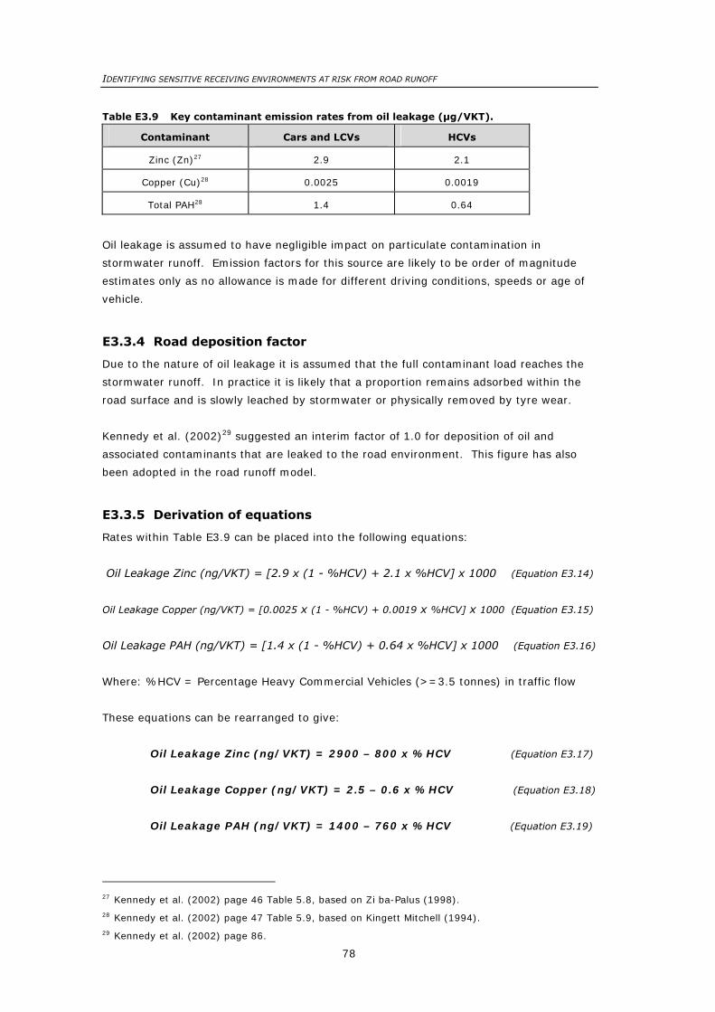
IDENTIFYING SENSITIVE RECEIVING ENVIRONMENTS AT RISK FROM ROAD RUNOFF
78
Table E3.9 Key contaminant emission rates from oil leakage (μg/VKT).
Contaminant Cars and LCVs HCVs
Zinc (Zn)27 2.9 2.1
Copper (Cu)28 0.0025 0.0019
Total PAH28 1.4 0.64
Oil leakage is assumed to have negligible impact on particulate contamination in
stormwater runoff. Emission factors for this source are likely to be order of magnitude
estimates only as no allowance is made for different driving conditions, speeds or age of
vehicle.
E3.3.4 Road deposition factor
Due to the nature of oil leakage it is assumed that the full contaminant load reaches the
stormwater runoff. In practice it is likely that a proportion remains adsorbed within the
road surface and is slowly leached by stormwater or physically removed by tyre wear.
Kennedy et al. (2002)29 suggested an interim factor of 1.0 for deposition of oil and
associated contaminants that are leaked to the road environment. This figure has also
been adopted in the road runoff model.
E3.3.5 Derivation of equations
Rates within Table E3.9 can be placed into the following equations:
Oil Leakage Zinc (ng/VKT) = [2.9 x (1 - %HCV) + 2.1 x %HCV] x 1000 (Equation E3.14)
Oil Leakage Copper (ng/VKT) = [0.0025 x (1 - %HCV) + 0.0019 x %HCV] x 1000 (Equation E3.15)
Oil Leakage PAH (ng/VKT) = [1.4 x (1 - %HCV) + 0.64 x %HCV] x 1000 (Equation E3.16)
Where: %HCV = Percentage Heavy Commercial Vehicles (>=3.5 tonnes) in traffic flow
These equations can be rearranged to give:
Oil Leakage Zinc (ng/VKT) = 2900 – 800 x %HCV (Equation E3.17)
Oil Leakage Copper (ng/VKT) = 2.5 – 0.6 x %HCV (Equation E3.18)
Oil Leakage PAH (ng/VKT) = 1400 – 760 x %HCV (Equation E3.19)
27 Kennedy et al. (2002) page 46 Table 5.8, based on Zi ba-Palus (1998). 28 Kennedy et al. (2002) page 47 Table 5.9, based on Kingett Mitchell (1994). 29 Kennedy et al. (2002) page 86.

APPENDIX E
79
E3.4 Exhaust emissions
E3.4.1 Introduction
Combustion of fuels in a vehicle engine generates exhaust gases and particulate matter.
If these emissions deposit on the roadway, or are washed out of the atmosphere by rain,
they enter the road’s stormwater runoff, and contribute to the contaminant load.
The methodology used to derive emission rate for contaminants from exhaust emissions
is discussed below.
E3.4.2 Particle emission rates
There have been extensive studies conducted on the nature of particle emissions from
vehicle exhausts. Most of these have focussed on fine particulate (PM10) as this size
fraction presents the greatest health risk from inhalation into the lungs. However, PM10
behaves like a gas and is mixed by turbulence and dispersed downwind from the road
corridor. Emission rates for larger particulate matter from vehicle exhausts, which are
likely to deposit on the road surface and contribute to road runoff, are generally not
available. Consequently the discussion below relates to PM10 data.
The MoT Vehicle Fleet Emissions Model (VFEM) produces rates for particulate matter
(PM10), expressed for four different road types and three traffic conditions (see Table
E3.10). These rates are weighted averages for the typical vehicle operating in the New
Zealand fleet in 2001. Classification of road type and traffic condition is defined in Annex
E2. (Note: due to the minor contribution of exhaust emissions to stormwater runoff,
separate rates for heavy and light vehicles were not considered necessary.)
Table E3.10 PM10 emission rates (g/km) from the MoT VFEM30.
Road type Free flow Interrupted Congested
Central Urban 0.215 0.267 0.339
Motorway 0.223 0.158 0.173
Rural 0.172 0.166 0.198
Suburban 0.185 0.208 0.253
E3.4.3 Contaminant emission rates from exhaust emissions
Kennedy et al. (2002) concluded from a review of the literature that there was insufficient
published data to establish clear relationships between the mass of PM10 emitted and the
concentration of contaminants in particulate matter from vehicle exhausts. As such,
emission rates for zinc, copper and PAH in exhaust emissions, as assumed by Kennedy et
al. (2002), are independent of the rates of emission of PM10 (and consequently particulate
in road runoff).
30 VFEM rates for 2001 vehicle fleet (model as at October 2005).

IDENTIFYING SENSITIVE RECEIVING ENVIRONMENTS AT RISK FROM ROAD RUNOFF
80
Table E3.11 lists the values cited by Kennedy et al. (2002) which have also been adopted
in the road runoff model.
Table E3.11 Key contaminant emission rates from exhaust emissions (μg/VKT).
Contaminant Light vehicles Heavy vehicles
Zinc 4631 62032
Copper32 15 88
Total PAH33 916 2358
The rates for total PAH are derived from a subset of hydrocarbons listed in Table 7.22 of
Kennedy et al. (2002). The listed rates for all contaminants are indicative as published
emission data for such chemical species are extremely variable between studies.
E3.4.4 Road deposition factor
Due to the rapid dispersal of exhaust emissions, most contaminants released from this
source do not deposit on the road surface directly from the roadway. Nevertheless, a
fraction of particulate from vehicle emissions dispersed in the atmosphere may
subsequently be washed out to the roadway by precipitation, along with other suspended
matter.
Kennedy et al. (2002) identified an interim road deposition factor of 0.05 for particles
associated with vehicle exhaust emissions34 and this factor has been adopted in the road
runoff model.
E3.4.5 Derivation of equations
Equations for contaminant loading in stormwater runoff can be derived from Tables E3.10
and E3.11:
Exhaust Particulate (mg/VKT) = 0.05 x E x M x 1000 (Equation E3.20)
Exhaust Zinc (ng/VKT) = 0.05 x [46 x (1 - %HCV) + 620v%HCV] x 1000 (Equation E3.21)
Exhaust Copper (ng/VKT) = 0.05 x [15 x (1 - %HCV) + 88 x %HCV] x 1000
(Equation E3.22)
Exhaust PAH (ng/VKT) = 0.05 x [916 x (1 - %HCV) + 2358 x %HCV] x 1000
(Equation E3.23)
31 Kennedy et al. (2002) page 75 Table 7.21, based on Gertler et al. (2002). 32 Kennedy et al. (2002) page 75 Table 7.21, based on Norbeck et al. (1998). 33 Kennedy et al. (2002) page 75 Table 7.22, based on Norbeck et al. (1998). 34 Kennedy et al. (2002) page 87.

APPENDIX E
81
Where:
EPM = Exhaust PM10, selected from Table E3.10
%HCV = Percentage Heavy Commercial Vehicles (>=3.5 tonnes) in traffic flow
Rearranging these equations gives:
Exhaust Particulate (mg/VKT) = 50 x EPM (Equation E3.24)
Exhaust Zinc (ng/VKT) = 2300 + 28700 x HCV (Equation E3.25)
Exhaust Copper (ng/VKT) = 750 + 3650 x %HCV (Equation E3.26)
Exhaust PAH (ng/VKT) = 45800 + 72100 x %HCV (Equation E3.27)
E3.5 Road surface wear
E3.5.1 Introduction
Tyres wear due to the frictional forces between them and the road surface. Conversely,
the road surface is also abraded by the movement of vehicles, producing additional
particulate and associated contaminant loading.
The emission rate for contaminants from road surface abrasion is derived from the wear
rate and road surface composition, as discussed below. Since the vast majority of traffic
to be assessed by this model will be travelling on bitumen/aggregate sealed roads,
analysis has been limited to this road type.
E3.5.2 Road surface wear rate
Kennedy et al. (2002) proposed a methodology for calculating road surface (bitumen and
aggregate) wear based on design life35 :
W x D x %B x ρB x 105 W x D x %A x ρA x 105 BW =
Yd x 365 x AADT AW =
Yd x 365 x AADT
(Equations E3.28 and E3.29)
Where:
BW = total bitumen wear (g/VKT)
AW = total aggregate wear (g/VKT)
W = width of wear, cm (assumed to be 100cm)
D = depth worn, cm (assumed to be 0.85cm)
%B = % of wear composed of bitumen (assumed to be 50%)
%A = % of wear composed of aggregate (assumed to be 50%)
ρB = density of bitumen (assumed to be 1 g/cm3)
35 Kennedy et al. (2002) page 82.

IDENTIFYING SENSITIVE RECEIVING ENVIRONMENTS AT RISK FROM ROAD RUNOFF
82
ρA = density of aggregate (assumed to be 2.7 g/cm3)
Yd = design life in years
AADT = annual average daily traffic on the road section
With the above assumed values, the wear of bitumen and aggregate simplify to:
11644 BW =
Yd x 365 x AADT (Equation E3.30)
31348 AW =
Yd x 365 x AADT (Equation E3.31)
The calculation of road seal design life, Yd, is based on the number of layers present in
the seal 36:
For single coat seals:
Yd = 4.916 + 1.68ALD – (1.03 + 0.219ALD) log(elv) (Equation E3.32)
For multilayer seals:
Yd = 14.87 + ALD – 3.719 log(elv) (Equation E3.33)
Where:
Yd = design life in years
elv = equivalent light vehicles/lane/day
ALD = average least dimension of the sealing chip in mm used on the section
(for multilayer seals the larger ALD is used)
(Equation E3.34)
Where:
AADT = annual average daily traffic on the road section
Lanes = number of lanes across whole road
%HCV = percentage heavy commercial vehicles
36 Transit New Zealand Specification TNZ P/17:2002.
⎟⎠⎞
⎜⎝⎛ +=
100)(%91 HCV
LanesAADTelv

APPENDIX E
83
E3.5.3 Road surface composition
Bitumen wear particles contain a range of organic and inorganic substances that may be
liberated into road runoff. Table E3 12 details the concentration in bitumen of the key
contaminants considered in this model. (Note: worn aggregate is considered inert and
therefore does not contribute to the concentration of contaminants in stormwater.)
Table E3.12 Concentration of contaminants in bitumen wear particles37.
Contaminant Concentration
(mg/kg)
Zinc 54
Copper 46
Total PAH 10
E3.5.4 Road deposition factor
Wind (local and vehicle derived turbulence) will transport a portion of road wear particles
outside the road corridor. Nevertheless, Kennedy et al. (2002) made the conservative
assumption that all road wear material is available for stormwater runoff38 and this
deposition factor of 1.0 has also been adopted in the road runoff model.
E3.5.5 Derivation of equations
Bitumen wear is likely to create fine particles capable of becoming suspended solids
within the stormwater. The character of aggregate wear particles is more diverse, with a
mixture of a fine fraction, due to the erosion of the aggregate itself, and entire aggregate
pieces, that are released with the removal of bitumen binder. Thus, a proportion of
aggregate ‘particles’ will be incapable of suspension in the runoff. However, the intact
aggregate fragments can create a loading on the stormwater system, especially treatment
devices such as catchpits.
With limited research available regarding the exact nature of road surface wear, it was
assumed that the total wear rate of both bitumen and aggregate contributed to the
loading of solid material in road runoff. This conservative approach will tend to
overestimate the suspended solid load in storm runoff.
However, due to the nature of the design life equation, this methodology will produce a
highly exaggerated estimate of road wear pollution loading for carriageways with less
than 2,000 AADT. It is proposed that road wear be ignored for streets with less than
2,000 vehicle movements per day.
37 Kennedy et al. (2002) page 83, based on Kennedy & Gadd (2003). 38 Kennedy et al. (2002) page 87.

IDENTIFYING SENSITIVE RECEIVING ENVIRONMENTS AT RISK FROM ROAD RUNOFF
84
On this basis, the combined aggregate and bitumen wear rate equations above are
summed to give (for AADT >= 2,000):
43082000 Road Surface Particulate Matter (mg/VKT) =
Yd x AADT (Equation E3.35)
Combination of the bitumen wear rate and the contaminant concentrations in Table E3.12
produces the following equations (for AADT >= 2,000):
628776000 Road Surface Zinc (ng/VKT) =
Yd x AADT (Equation E3.36)
535624000 Road Surface Copper (ng/VKT) =
Yd x AADT (Equation E3.37)
116440000 Road Surface PAH (ng/VKT) =
Yd x AADT (Equation E3.38)
E4 Model description
This section provides a summary description of the vehicle contaminant load model for
road runoff (`the model’) under the following subsections:
Section E4.1 - Model overview
Section E4.2 - Contaminant load model equations
Section E4.3 - Contaminant load model inputs
Section E4.4 - Treatment of road runoff
Section E4.5 - User inputs
Section E4.6 - Worked examples
Benefit values (willingness to pay) for removal of the four key contaminants from
stormwater, thus providing a common unit of comparison for ranking purposes, are
included in Section E4.4.
An initial validation of the model using published data is given in Section E5.
E4.1 Model overview
The model is an Excel-based programme which estimates total mass loadings (kg/VKT) of
specific vehicle-derived contaminants in road runoff. The pollutants are particulate, zinc,
copper and polyaromatic hydrocarbons (PAH) as these are the primary vehicle-derived
contaminants of interest in terms of road runoff. Figure E4.1 gives a schematic of the
model process.

APPENDIX E
85
The contaminant load per VKT is calculated using the overall contaminant load model
equations given in Section E4.2. By multiplying the contaminant loading per VKT by the
road section AADT and length, the model creates an estimate of the total annual load of
contaminants in runoff generated on that section of road prior to any containment or
treatment device.
Depending on the treatment device or stormwater containment method in place, the
contaminant loading reaching any waterbody can be significantly reduced. Contaminant
load in the outfall of the device is a function of the quantity of flow treated and the
contaminant reduction efficiency. Multiplying the total road contaminant load by these
removal rates (detailed in Section E4.4) gives an approximation of the annual load of
contaminants in road runoff i.e. discharged from the road network outfall.
(Note: this load may undergo further dilution/attenuation along a discharge pathway
before it impacts a sensitive receiving environment; alternatively a direct impact may
occur when the load is discharged directly to a sensitive waterbody. The pathway
attenuation factor is to be considered in a subsequent stage of this research project.)
Figure E4.1 Schematic of contaminant load calculation.
Contaminants produce a range of environmental impacts and, as described in Section
E4.4, the perceived value that the community places on these impacts varies. By
multiplying the individual road runoff contaminant loads in runoff by their perceived
financial values, and summing the contributions, an indicative contaminant loading value
Contaminant Load
(kg/VKT)
Traffic Flow
(AADT)
Road Length (km)
Total Annual Road Contaminant Load
Road Runoff
Contaminant Load
(kg/year) Indicative
Contaminant
Load Value ($)
% Flow Not
Treated
% Flow Treated *
(1 - % Contaminant Reduction/100)
+
Relative Contaminant
Value ($/kg/year)
X
X
X
X

IDENTIFYING SENSITIVE RECEIVING ENVIRONMENTS AT RISK FROM ROAD RUNOFF
86
is derived. This concept has potential value for ranking road or road networks in terms of
pollutant load but its application and use have not been further developed under this
project.
The model is designated a `vehicle contaminant load model’ as it is restricted to
emissions from road vehicles – it does not quantify pollutants in road runoff that arise
from other sources e.g. open land, urban or industrial discharges and which contribute to
the overall stormwater pollutant load. However, the model is capable of distinguishing
the relative contributions of contaminant loads from different road types (e.g. state
highways vs. local roads within a catchment) that may affect a given receiving
environment.
E4.2 Contaminant load model equations
The equations derived for each vehicle-based contaminant source (detailed in Section E3)
have been combined to produce the four key model equations used for estimating
contaminant loads in road runoff for particulate matter (PM), zinc, copper and PAH:
Where AADT < 2,000:
PM(mg/VKT) = 7.7Bi + 82.4Ti + %HCV[20.3Bi + 362.4Ti] + 50 x EPM (Equation E4.1)
Zinc(µg/VKT) = 5.2 +12.5Bi + 684.7Ti + %HCV[33.1Bi + 3011.5Ti + 29.9]
(Equation E4.2)
Copper(µg/VKT) = 0.753 +38.5Bi + 0.0824Ti + %HCV[101.5Bi + 0.362Ti + 3.649]
(Equation E4.3)
PAH(µg/VKT) = 47.2 +0.123Bi + 18.6Ti + %HCV[0.325Bi + 81.9Ti + 71.3]
(Equation E4.4)
Where AADT >= 2,000:
4308200 PM(mg/VKT) = 7.7Bi + 82.4Ti + %HCV[20.3Bi + 362.4Ti] + 50 x EPM +
Yd x AADT
(Equation E4.5)
628776 Zinc(µg/VKT) = 5.2 +12.5Bi + 684.7Ti + %HCV[33.1Bi + 3011.5Ti + 29.9]+
Yd x AADT
(Equation E4.6)
Copper(µg/VKT) =
535624 0.753 +38.5Bi + 0.0824Ti + %HCV[101.5Bi + 0.362Ti + 3.649]+
Yd x AADT
(Equation E4.7)
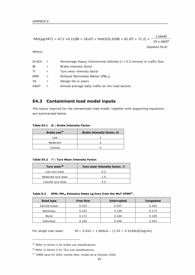
APPENDIX E
87
116440 PAH(µg/VKT) = 47.2 +0.123Bi + 18.6Ti + %HCV[0.325Bi + 81.9Ti + 71.3] +
Yd x AADT
(Equation E4.8)
Where:
%HCV = Percentage Heavy Commercial Vehicles (>=3.5 tonnes) in traffic flow
Bi = Brake intensity factor
Ti = Tyre wear intensity factor
EPM = Exhaust Particulate Matter (PM10)
Yd = Design life in years
AADT = Annual average daily traffic on the road section
E4.3 Contaminant load model inputs
The inputs required for the contaminant load model, together with supporting equations,
are summarised below:
Table E4.1 Bi : Brake Intensity Factor.
Brake use39 Brake intensity factor, Bi
Low 1
Moderate 3
Intense 4
Table E4.2 Ti : Tyre Wear Intensity Factor.
Tyre wear40 Tyre wear intensity factor, Ti
Low tyre wear 0.2
Moderate tyre wear 1.6
Intense tyre wear 3.3
Table E.3 EPM: PM10 Emission Rates (g/km) from the MoT VFEM41.
Road type Free flow Interrupted Congested
Central Urban 0.215 0.267 0.339
Motorway 0.223 0.158 0.173
Rural 0.172 0.166 0.198
Suburban 0.185 0.208 0.253
For single coat seals: Yd = 4.916 + 1.68ALD – (1.03 + 0.219ALD)log(elv)
39 Refer to Annex 2 for brake use classifications. 40 Refer to Annex 2 for Tyre use classifications. 41 VFEM rates for 2001 vehicle fleet, model as at October 2005.

IDENTIFYING SENSITIVE RECEIVING ENVIRONMENTS AT RISK FROM ROAD RUNOFF
88
For multilayer seals: Yd = 14.87 + ALD – 3.719log(elv)
Where:
Yd = design life in years
elv = equivalent light vehicles/lane/day
ALD = average least dimension of the sealing chip in mm used on the section
(Note: for multilayer seals the largest value of ALD is used.)
Where:
AADT = annual average daily traffic on the road section
Lanes = number of lanes
%HCV = percentage heavy commercial vehicles
E4.4 Treatment of road runoff
E4.4.1 Introduction
The equations described in Section E4.2 enable an estimate to be made of the
contaminant load (i.e. particulate matter, zinc, copper and PAH in mg/year) deposited on
a road surface from a given set of traffic and road attributes.
However, the actual contaminant load that leaves the highway in road runoff will be
determined by the nature of the highway drainage infrastructure, including any treatment
devices. The type of drainage infrastructure (e.g. swale or kerb/channel) plays a key role
in controlling the pollutant load and therefore the risk from contaminants in stormwater
runoff.
This section describes how the runoff model takes account of the existing (or proposed)
stormwater treatment device in order to estimate the contaminant load that is actually
discharged to the receiving environment.
E4.4.2 Stormwater treatment devices
Hartwell & Welsh (2005) conducted a detailed literature review of the most common
stormwater containment and treatment devices that are used for road runoff. A list with
a description of each of these treatment devices is given in Annex E3. Further details on
the design guidelines for each type are to be found in ARC (2003).
E4.4.3 Treatment efficiencies
Hartwell & Welsh (2005) also included a review of the contaminant retention (removal)
efficiency of a range of stormwater treatment devices. A summary is given in Table E4.4.
The flow treatment figures are approximate and refer to the percentage of influent by that
is treated by the device. It was assumed that the reduction rates for PAH are the same
⎟⎠⎞
⎜⎝⎛ +=
100)(%91 HCV
LanesAADTelv

APPENDIX E
89
as those reported by Hartwell & Welsh (2005) for TPH. This is a reasonable assumption
as PAH are a subgroup of Total Petroleum Hydrocarbons (TPH).
The removal efficiencies for the four contaminants provide the typical mass reduction that
is achievable for the device, assuming that this is well maintained and correctly sized for
the expected throughput. These rates have been used in the runoff model to take
account of any treatment device on the section of highway in estimating pollutant loads
discharged to the receiving environment from the road corridor.
The flow treatment figures are approximate and refer to the percentage of influent by that
is treated by the device. It was assumed that the reduction rates for PAH are the same
as those reported by Hartwell & Welsh (2005) for Total Petroleum Hydrocarbons . This is
a reasonable assumption as PAH are a subgroup of TPH.
Table E4.4 Approximate retention efficiency of various stormwater treatment devices42.
Retention efficiency total mass (%) Device
No. Treatment device
Annual flow
treated
%
Suspended
solids Zinc Copper PAH 43
1 Culvert/direct discharge 100 0 0 0 0
2 Catchpits (average) 44 100 64 29 36 10
3 Dry Water Quality Pond 100 63 27 41 10
4 Wet Water Quality Pond 100 77 36 51 10
5 Wet Extended Detention Pond 100 80 41 54 10
6 Constructed Wetland 100 77 54 69 10
7 Swale 100 75 47 57 47
8 Bio-retention Device
(80% rain garden; 20% swale) 100 83 59 62 65
9 Rain Garden 90 84 51 63 48
10 Proprietary Device Type 1(a)
- Gross Pollutant Traps 74 30 9 18 10
11 Proprietary Device Type 2(b)
- Filtration Systems 90 84 44 59 48
12 Proprietary Device Type 3(c)
- Catchpit Filter Systems 90 42 13 25 10
Note: (a) Examples include Downstream Defender, CDS, Ecosol, CleansAll; (b) Examples include Sand Filter, Storm Filter; (c) Examples include Enviropod, Ecosol 100, FloGuard
The removal efficiencies for the four contaminants provide the typical mass reduction that
is achievable for the device, assuming that this is well maintained and correctly sized for
the expected throughput. These rates have been used in the runoff model to take
account of any treatment device on the section of highway in estimating pollutant loads
discharged to the receiving environment from the road corridor.
42 From Hartwell & Welsh (2005) p36 Table 5.2, unless stated otherwise. 43 Listed values are for Total Petroleum Hydrocarbons and are assumed the same for PAH. 44 Derived from Timperley et al. (2005) and Ng et al. (2003).

IDENTIFYING SENSITIVE RECEIVING ENVIRONMENTS AT RISK FROM ROAD RUNOFF
90
E4.4.4 Relative contaminant values
Hartwell & Welsh (2005) produced benefit values based on the reduction of individual
contaminants in road runoff by various stormwater treatment devices. This was derived
from a Contingent Valuation approach to determine willingness-to-pay and impact
weightings based on survey questionnaires of communities in Rodney District, Waitakere
City and North Shore City. The survey found that 44% of households were in favour of
treating runoff from roads at a cost of $1,000 per household per year. The benefit values
for unit reduction of each of the key contaminants (in $/kg/year) are given in Table E4.5.
Table E4.5 Weighted benefit values for contaminant reduction45.
Contaminant Benefit value
$/kg/year
Suspended solids 44
Zinc 37,801
Copper 144,818
PAH46 106,871
Of the four contaminants considered, the lowest benefit is derived for suspended solids
and the highest is for copper. Reduction of copper has a perceived benefit of almost four
times that of zinc. Caution is needed in application of these benefit values. As the
authors point out, TPH was highly weighed by the public, possibly “because oils are very
visual and easy to connect these to roads. It is harder for the public to make the link
between roads and metals such as zinc and copper”.
With these limitations in mind, the benefit values can be used to add together the
differing emission loads of the four key contaminants derived by the runoff model to
provide an overall benefit for the road network. The runoff model includes the benefit
value calculation for ranking and comparative purposes only.
(Note: the monetary benefit derived from these values does not equate to the cost of
stormwater treatment for the relevant road section; it is merely the community’s
perceived value expressed in monetary terms of stormwater treatment in improving the
receiving environment.)
E4.5 User inputs
User-specified inputs that are required to run the model are listed in Table E4.6. The
column `RAMM Table’ indicates the equivalent designation of each variable (where
appropriate) in the RAMM database. The column `Modification’ refers to instructions on
how to adjust the RAMM input data to run the model or suit the user preference.
45 Hartwell & Welsh (2005) p39 Table 6.3. 46 Values for Total Petroleum Hydrocarbons, and assumed the same for PAH.

APPENDIX E
91
Table E4.6 User inputs to the model.
Variable name RAMM table(a) Modification
AADT (vehicle/day) Traffic [use ADT] None
Road Type Carriageway Allocate RAMM classifications to road type groups
defined in Annex E2
Level of Service (LoS) - Calculate and apply groups defined in Annex E2
HCV (%) Carriageway None
No of Lanes Carriageway None
Road Length (km) Carriageway None
Horizontal Terrain
(deg/km)
High speed geometry Convert radians to degrees via trigonometry
Vertical Terrain (m/km) High speed
geometry Convert units
No of Seal Layers Surface structure Allocate RAMM information as either single or
multilayer
ALD (mm) Surface structure None
Treatment Drainage
Insert device number (Table E4.1) or assign
nearest device to road section - alternative
treatment devices may need to be stipulated
from local knowledge
(a) New Zealand’s Road Asset Maintenance Management system
E4.6 Worked examples
Table E4.4 contains three worked examples of the road runoff contaminant load model.
These illustrates both the model input and output data and range of contaminant loads for
the four main pollutants – particulate matter, zinc, copper and PAH.
E4.6.1 Example A
Example A compares the effects of varying traffic flows on a typical suburban road under
three increasing Levels of Service: 10,000 AADT (free flow), 15,000 (interrupted) and
20,000 (congested). All other variables remain constant. The runoff is discharged
through a catchpit.
The example demonstrates the increase in contaminant load as a function of traffic flow.
However the relationship is not linear. A doubling of traffic from 10,000 to 20,000 AADT
increases the copper discharge by a factor of about 7 and the zinc discharge by a factor of
about 30. This is due to the increased level of congestion with the higher traffic flows and
consequent increase in vehicle braking, acceleration and tyre wear.
E4.6.2 Example B
This example compares the effects of pollutant load on two different road types (suburban
road and a motorway), both carrying the same level of traffic. The suburban road has 2
IDENTIFYING SENSITIVE RECEIVING ENVIRONMENTS AT RISK FROM ROAD RUNOFF
92
lanes while the motorway has six. All other variables remain constant. The runoff is
discharged without treatment.
In this case the heavy metal contaminant load in the road runoff is very similar. The
slight reduction for motorway values is due to a lower equivalent light vehicles per lane
per day (`elv’ term in Equation E3.34) and hence a slightly higher design life for the road
(`Yd' term in Equation E4.6 for zinc, and Equation E4.7 for copper). This results in a
small reduction in surface wear of the motorway compared with the suburban road. The
particulate matter load for the two road types is similar but in this case the difference in
PM10 emission rates for motorway and suburban roads (`EPM’ term in Equation E4.5) has
a further contributory effect. In practice these differences are negligible.
E4.6.3 Example C
Example C compares the effects of varying road conditions (bends and hills) on the
contaminant load for two sections of rural highway, one hilly and the other mountainous
(see terrain classification in Table A2.3), but each with identical levels of traffic and
%HCVs. All other variables remain constant. The runoff is discharged without treatment.
The example demonstrates the increase in contaminant load as a function of more
mountainous terrain with a larger number of tighter bends causing more braking (as seen
by 32% more copper) and much greater tyre wear (as seen by a doubling of the zinc).
Other pollutants also increase in the rugged mountain section compared with the hilly
road.
E4.6.4 Example D
The final example compares the contaminant loads from identical roads with and without
treatment. The suburban road with 10,000 AADT and a catchpit (column 1) is compared
with the same road with no stormwater treatment device (column 4), all other factors
being identical.
The example demonstrates the importance of catchpits in removing suspended sediment
and heavy metals. The average catchpit has an approximate retention efficiency of 64%
for suspended solids (see Table E4.7 with corresponding figures for copper of 36% and
zinc 29%). Retention of PAH is low at only 10%.

APPENDIX E
93
Table E4.7 Vehicle contaminant load model - input and output data for example road scenarios.
Attribute Example A
(Change in traffic flow)
Example B
(Change in road type)
Example C
(Change in road condition)
Model Input 1 2 3 4 5 6 7
Road Type Suburban Suburban Suburban Suburban Motorway Rural Highway Rural Highway
Level of Service (LoS) 1: Free Flow 2: Interrupted 3: Congested 1: Free Flow 1: Free Flow 1: Free Flow 1: Free Flow
AADT (veh/day) 10,000 15,000 20,000 10,000 10,000 10,000 10,000
HCV (%) 10% 10% 10% 10% 10% 15% 15%
No of Lanes 2 2 2 2 6 2 2
Road Length (km) 1 1 1 1 1 1 1
Horizontal Terrain (deg/km) 10 10 10 10 10 55 250
Vertical Terrain (m/km) 25 25 25 25 25 55 65
No of Seal Layers 1 1 1 1 1 1 1
ALD (mm) 8.5 8.5 8.5 8.5 8.5 8.5 8.5
Treatment Catchpit Catchpit Catchpit None(a) None(a) Culvert Culvert
Model Output
Particulates (g/day) 1,981 3,182 5,226 5,502 4,811 7,675 10,107
Zinc (mg/day) 1,623 17,447 47,270 2,286 2,275 18,878 38,372
Copper (mg/day) 359 1,457 2,555 561 552 1,690 2,230
PAH (mg/day) 551 1,332 2,594 612 610 1,092 1,619
Relative contaminant value47 1 10.7 29.0 1.4 1.4 11.6 23.6
(a) No treatment device - direct discharge to receiving environment (equivalent to ‘culvert’ in Table E4.4).
Example D (see text) compares columns 1 and 4.
47 Based on Weighted benefit value of contaminant reduction, Table E4.5.
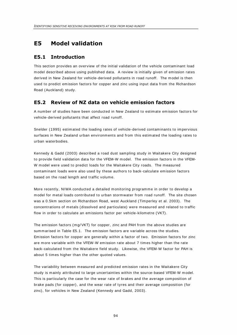
IDENTIFYING SENSITIVE RECEIVING ENVIRONMENTS AT RISK FROM ROAD RUNOFF
94
E5 Model validation
E5.1 Introduction
This section provides an overview of the initial validation of the vehicle contaminant load
model described above using published data. A review is initially given of emission rates
derived in New Zealand for vehicle-derived pollutants in road runoff. The model is then
used to predict emission factors for copper and zinc using input data from the Richardson
Road (Auckland) study.
E5.2 Review of NZ data on vehicle emission factors
A number of studies have been conducted in New Zealand to estimate emission factors for
vehicle-derived pollutants that affect road runoff.
Snelder (1995) estimated the loading rates of vehicle-derived contaminants to impervious
surfaces in New Zealand urban environments and from this estimated the loading rates to
urban waterbodies.
Kennedy & Gadd (2003) described a road dust sampling study in Waitakere City designed
to provide field validation data for the VFEM-W model. The emission factors in the VFEM-
W model were used to predict loads for the Waitakere City roads. The measured
contaminant loads were also used by these authors to back-calculate emission factors
based on the road length and traffic volume.
More recently, NIWA conducted a detailed monitoring programme in order to develop a
model for metal loads contributed to urban stormwater from road runoff. The site chosen
was a 0.5km section on Richardson Road, west Auckland (Timperley et al. 2003). The
concentrations of metals (dissolved and particulate) were measured and related to traffic
flow in order to calculate an emissions factor per vehicle-kilometre (VKT).
The emission factors (mg/VKT) for copper, zinc and PAH from the above studies are
summarised in Table E5.1. The emission factors are variable across the studies.
Emission factors for copper are generally within a factor of two. Emission factors for zinc
are more variable with the VFEW-W emission rate about 7 times higher than the rate
back-calculated from the Waitakere field study. Likewise, the VFEM-W factor for PAH is
about 5 times higher than the other quoted values.
The variability between measured and predicted emission rates in the Waitakere City
study is mainly attributed to large uncertainties within the source-based VFEM-W model.
This is particularly the case for the wear rate of brakes and the average composition of
brake pads (for copper), and the wear rate of tyres and their average composition (for
zinc), for vehicles in New Zealand (Kennedy and Gadd, 2003).
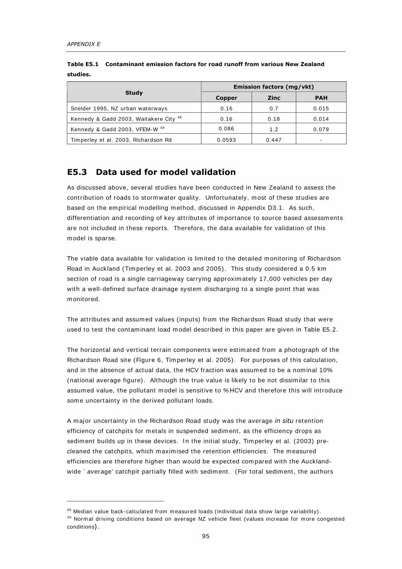
APPENDIX E
95
Table E5.1 Contaminant emission factors for road runoff from various New Zealand
studies.
Emission factors (mg/vkt) Study
Copper Zinc PAH
Snelder 1995, NZ urban waterways 0.16 0.7 0.015
Kennedy & Gadd 2003, Waitakere City 48 0.16 0.18 0.014
Kennedy & Gadd 2003, VFEM-W 49 0.086 1.2 0.079
Timperley et al. 2003, Richardson Rd 0.0593 0.447 -
E5.3 Data used for model validation
As discussed above, several studies have been conducted in New Zealand to assess the
contribution of roads to stormwater quality. Unfortunately, most of these studies are
based on the empirical modelling method, discussed in Appendix D3.1. As such,
differentiation and recording of key attributes of importance to source based assessments
are not included in these reports. Therefore, the data available for validation of this
model is sparse.
The viable data available for validation is limited to the detailed monitoring of Richardson
Road in Auckland (Timperley et al. 2003 and 2005). This study considered a 0.5 km
section of road is a single carriageway carrying approximately 17,000 vehicles per day
with a well-defined surface drainage system discharging to a single point that was
monitored.
The attributes and assumed values (inputs) from the Richardson Road study that were
used to test the contaminant load model described in this paper are given in Table E5.2.
The horizontal and vertical terrain components were estimated from a photograph of the
Richardson Road site (Figure 6, Timperley et al. 2005). For purposes of this calculation,
and in the absence of actual data, the HCV fraction was assumed to be a nominal 10%
(national average figure). Although the true value is likely to be not dissimilar to this
assumed value, the pollutant model is sensitive to %HCV and therefore this will introduce
some uncertainty in the derived pollutant loads.
A major uncertainty in the Richardson Road study was the average in situ retention
efficiency of catchpits for metals in suspended sediment, as the efficiency drops as
sediment builds up in these devices. In the initial study, Timperley et al. (2003) pre-
cleaned the catchpits, which maximised the retention efficiencies. The measured
efficiencies are therefore higher than would be expected compared with the Auckland-
wide `average’ catchpit partially filled with sediment. (For total sediment, the authors
48 Median value back-calculated from measured loads (individual data show large variability). 49 Normal driving conditions based on average NZ vehicle fleet (values increase for more congested conditions).

IDENTIFYING SENSITIVE RECEIVING ENVIRONMENTS AT RISK FROM ROAD RUNOFF
96
Table E5.2 Modelled attributes and values from Richardson Road study.
Attribute Assumed value
AADT 17,354
Road Type SU
LoS 2: Interrupted
% HCV 10%
# of Lanes 2
Horizontal Terrain (degrees/km) <50
Vertical Terrain (m/km) <45
# of Seal Layers 1
ALD (mm) 8.5
Treatment Catchpit (average)
estimated that this would equate to about 75% retention compared with an in situ figure
of about 60%.)
In the subsequent study (Timperley et al. 2005), reduced retention efficiencies were
developed for the more realistic situation of partially filled catchpit (the `average’
catchpit). The pollutant loads actually entering the stormwater system for these
`average’ catchpits are correspondingly higher.
The catchpit retention efficiencies used in this model validation are those given in Table
E4.1 for an `average’ catchpit. These equate to a partially filled catchpit derived from
data in Ng et al. (2003) and Timperley et al. (2005).
E5.4 Model predictions compared with field study
Contaminant load rates (in mg/VKT for total copper and total zinc) derived from applying
the contaminant load model to the Richardson Road site data are given in Table E5.3.
These are compared with results for total metals (sum of dissolved and particulate
fractions) reported in Timperley et al. (2005), assuming an average catchpit efficiency
from their model predictions at the same site. Also shown are data for the VFEM-W
model (Kennedy & Gadd 2003).
A direct comparison may be made between predictions for this model and the Timperley
model, both assuming an `average’ catchpit (i.e. one in use and partially filled with
sediment), as shown by data highlighted (*) in Table E5.3. The emission factors for
copper are within a factor of two while the emission factors for zinc are more divergent
(within a factor of four). In both cases, the model in this study overestimates the
contaminant load compared with Timperley et al. (2005).
As discussed in Section D3.1, the contaminant load model developed in this project (like
the MoT’s VFEM-W model) is a source-based model developed from vehicle emission

APPENDIX E
97
Table E5.3 Comparison of model predictions of emission factors for Richardson Road,
Auckland.
Study Total copper
(mg/VKT)
Total zinc
(mg/VKT)
This Model - average catchpit LoS = 1 0.05 0.23
This Model - average catchpit LoS = 2 0.15 * 1.6 *
This Model - average catchpit LoS = 3 0.20 3.3
Timperley et al. 2005 50 - average catchpit 0.078 * 0.45 *
Timperley et al. 2005 51 - clean catchpit 0.055 0.368
VFEM-W (normal driving conditions - LoS = 1) 52 0.086 1.2
VFEM-W (congested traffic – LoS = 3)52 0.12 2.3
Note: LoS = Level of Service (i.e. degree of traffic congestion – see Table A2.2).
* data comparable
factors derived from the MoT’s research programme, and based on source components
(e.g. zinc from tyres based on wear rates and tyre composition) and traffic/road
characteristics. The Timperley model is empirical where contaminant loads are derived
from correlating the measured concentrations of metals in road runoff to road traffic data
under actual field conditions. The results in Table E5.3 compare favourably, given the
different approaches used and the uncertainties in assumptions of both models.
The emission factors derived from the model (this study) are particularly sensitive to the
Level of Service (degree of traffic congestion). For example, copper shows a fourfold
increase in emission rates in moving from normal flows (LoS 1) to congested conditions
(LoS 3). The increase for zinc is even more marked (a factor of 14 for the same
comparison). The Level of Service has been estimated at a value of 2 for purposes of
comparing model outputs but the actual value may be less than 2. This limitation could
be overcome by replacing the discrete LoS bands with a continuous function relating
emission factors to vehicle speed.
The findings indicate that further refinement and calibration with field data is required
before the model may be used to estimate absolute pollutant loads in runoff from roads.
Notwithstanding these uncertainties, preliminary validation of the vehicle pollutant load
model developed in this study shows that it will find application in later stages of the
research project for comparative assessment of contaminant loads from different road
networks.
50 Timperley et al. (2005), p31, estimated for partially filled catchpits (reflecting likely in situ sediment retention efficiency). 51 Timperley et al. (2005), p29 Table 4, pre-cleaned catchpits (as per study). 52 Kennedy & Gadd (2003) Table 4.2.

IDENTIFYING SENSITIVE RECEIVING ENVIRONMENTS AT RISK FROM ROAD RUNOFF
98
E6 Conclusions and recommendations
E6.1 Conclusions
The following conclusions are drawn on the vehicle contaminant load model developed in
this study:
• A contaminant load model for road runoff has been developed for vehicle-derived
pollutants (copper, zinc, PAH and suspended solids). The model is based largely
on emission factors developed and published under the MoT’s research
programme on effects of transport on the aquatic environment. The model allows
user selection of stormwater treatment devices as part of the existing highway
drainage.
• Initial validation of the model for copper and zinc has been achieved by applying
the model to published field data and road characteristics for the Richardson Road
site in Auckland. The correlation between the predicted pollutant load rates from
the model (mg/VKT) is within a factor of two (copper) and four (zinc). In both
cases the model overestimates the contaminant load.
• The model output is particularly sensitive to the Level of Service (traffic
congestion) as this is currently incorporated in the model as three discrete bands.
A continuous function relating emission factors to vehicle speed would overcome
this limitation.
• There is considerable uncertainly in the derivation of emission factors in the
model, given the wide variability in source data, hence the model predictions
must be treated as only order of magnitude estimates of contaminant load.
• Based on these inherent limitations and uncertainties, the model should be used
to estimate contaminant loads from road networks on a comparative rather than
absolute basis.
E6.2 Recommendations
It is recommended that the following considerations be taken into account in development
of the risk-based SRE screening methodology that comprises the overall objective of this
project:
1) A simple screening of road networks based on VKT by sub-catchment be
considered in combination with criteria being developed for SRE sensitivity under
Stage 2 to identify sections of road with higher risk potential (Tier 1 screening
process).
2) The pollutant load model described in this report is applied to the identified higher
risk road sections to provide a more definitive and comparative measure of the risk

APPENDIX E
99
from road traffic, for taking forward in the SRE risk assessment process (Tier 2
assessment).
3) Further validation and sensitivity analysis of the contaminant load model is
undertaken to assess the limits of its application for estimating absolute
contaminant loads (outside the scope of this project).
E7 References
ARC 2003. Stormwater Management Devices: Design Guidelines Manual. Auckland
Regional Council Technical Publication No.10.
Bennett, C.R. & Greenwood, I.D. 2001. Volume Seven: Modelling road user and
environmental effects in HDM-4. In The Highway Development and Management
Series. Report to the International Study of Highway Development and Management
Tools, University of Birmingham.
Cadle, S.H. & Williams, R.L. 1978. Characterisation of tire emissions using an indoor
testing facility. Rubber Chemical Technology 51: 7.
Carpenter, P. & Cenek, P. 1999. Tyre wear modelling for HDM-4. Central Laboratories
Report, 98-529474. Report prepared for ISOHDM by Opus International Consultants
Limited, Central Laboratories, Lower Hutt.
Cha, S., Carter, P. & Bradow, R.L. 1983. Simulation of automobile brake wear dynamics
and estimation of emissions. SAE technical paper series 831036. Passenger car
meeting, Dearbon, Michigan June 6-9 1983. Society of Automotive Engineers.
Gertler, A.W., Gillies, J.A., Pierson, W.R., Rogers, C.F., Sagabiel, J.C., Abu-Allaban, M.,
Coulombe, W., Tarnay, L. & Cahill, T.A. 2002. Real world particulate matter and
gaseous emissions from motor vehicles in a highway tunnel. Research Report Number
107, Health Effects Institute.
Hartwell, S. & Welsh C. 2005. Development of a benefit evaluation technique applicable
to treatment of road runoff. Transfund New Zealand Research Report No. 264. 68pp.
Kennedy, P. & Gadd, J. 2003. Evaluation of road surface contaminant loadings in
Waitakere City for the development of the Vehicle Fleet Emission Model – Water.
Ministry of Transport, Wellington, New Zealand.
Kennedy, P., Gadd, J. & Moncrieff, I. 2002. Emission factors for contaminants released
by motor vehicles in New Zealand. Ministry of Transport, Wellington and
Infrastructure Auckland, New Zealand.
IDENTIFYING SENSITIVE RECEIVING ENVIRONMENTS AT RISK FROM ROAD RUNOFF
100
Kingett Mitchell, 1994. Used oil management in New Zealand. Report prepared by
Kingett Mitchell Ltd., Auckland, for the Used Oil Recovery Group.
Ministry of Transport 1998. Vehicle fleet emission model: New Zealand vehicle fleet
database and model development. Technical report compiled by the Ministry of
Transport, Wellington, New Zealand, in support of the Vehicle Fleet Emission Control
Strategy.
Moncrieff I. & Kennedy P. 2004. Road transport impacts on aquatic ecosystems: issues
and context for policy development. Prepared for Ministry of Transport, Wellington,
New Zealand.
Ng, W.H., Buckeridge, J.S. & Ockleston, G. 2003. Distribution of heavy metal
contaminants in road sediments. New Zealand Water and Waste Association, Third
South Pacific Conference on Stormwater and Aquatic Resource Protection, Auckland,
New Zealand.
Norbeck, J., Durbin, T. & Truex, T. 1998. Measurement of primary particulate matter
emissions from light-duty motor vehicles. CRC Project No. E-24-2. Center for
Environmental Research and Technology, University of California.
Rogge, W.F., Hildemann, L.M., Mazurek, M.A., Case, G.R. & Simoneit, B.R.T. 1993.
Sources of fine organic aerosol. 3. Road dust, tire debris and organometallic brake
lining dust: roads as sources and sinks. Environmental Science and Technology, 27:
636-651.
Snelder, T. 1995. Comparison of runoff quality from roads versus other urban landuses.
NIWA Consultancy Report No ARC60501: 1-16. National Institute of Water & Air,
Christchurch, New Zealand.
Transfund 2004. Amendment No. 8, Project Evaluation Manual PFM2.
Zi ba-Palus, J. 1998. Examination of used motor oils by flame AAS for criminalistic
purposes: a diagnostic study. Forensic Science International, 91: 171-179.

APPENDIX E
101
Annex E1 VKT split by vehicle type
An estimate of the VKT proportional splits for different vehicle types was taken from the
MoT’s Vehicle Fleet Emissions Model (VFEM), Table EA1.
The VFEM’s development has been dormant since 2002, and VKT estimates beyond 2001
are highly speculative. Hence, values for 2001 were used in this model. If the VFEM is
updated any improved data should be incorporated in this model.
Table EA1 VKT splits by vehicle type (2001).
Vehicle Size % of VKT % of VKT subtotals
Motorcycles - 0.35 -
Cars - 76.93 -
LCVs - 13.00 -
Total Light - - 90.28
HCVs Small 4.03 -
- Medium 1.66 -
- Large 4.03 -
Total Heavy - - 9.72

IDENTIFYING SENSITIVE RECEIVING ENVIRONMENTS AT RISK FROM ROAD RUNOFF
102
Annex E2 Definitions for road type, traffic condition and terrain
EA2.1 Definitions
The following section gives definitions for:
• Road Type • Traffic Condition (Level of Service) • Terrain
EA2.1.1 Road Type
The road type categories utilised in the model are outlined in Table EA2.1. Roads should
be assigned to the category that best exemplifies its nature. Accuracy in this area is not
critical to the operation of the model: the road type input is used primarily for the
selection of PM10 emissions, a minor contributor to suspended solid loading. The default
of ‘SU’ should be used in urban areas if further classification is not possible.
Table EA2.1 Road type.
Abbreviation Name Description53
MO Motorways
Essentially urban or urban fringe; characterised by limited
access design, grade separated intersections, multi-lane in
a relatively wide road reserve (includes urban State
Highways).
CU Central Urban
Roads
Central business areas, high frequency of signalised
intersection control and relatively low speeds, retail and
office land use in close proximity.
SU Suburban Roads Urban/suburban arterial/collector/distributor/local access
roads other than CU and MO.
RH Rural Highways
and local Roads
Rural highways: State highways, predominantly 2 lane main
connecting routes; relatively high percentage of heavy
traffic, some 3 lane sections on gradients and where
horizontal geometry is restricted.
Rural local roads: local authority, 2 lane, mainly distributor
and local access in nature.
53 Ministry of Transport (1998).
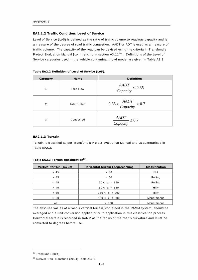
APPENDIX E
103
EA2.1.2 Traffic Condition: Level of Service
Level of Service (LoS) is defined as the ratio of traffic volume to roadway capacity and is
a measure of the degree of road traffic congestion. AADT or ADT is used as a measure of
traffic volume. The capacity of the road can be devised using the criteria in Transfund’s
Project Evaluation Manual [commencing in section A3.1154]. Definitions of the Level of
Service categories used in the vehicle contaminant load model are given in Table A2.2.
Table EA2.2 Definition of Level of Service (LoS).
Category Name Definition
1 Free Flow
2 Interrupted
3 Congested
EA2.1.3 Terrain
Terrain is classified as per Transfund’s Project Evaluation Manual and as summarised in
Table EA2.3.
Table EA2.3 Terrain classification55.
Vertical terrain (m/km) Horizontal terrain (degrees/km) Classification
< 45 < 50 Flat
> 45 < 50 Rolling
< 45 50 < x < 150 Rolling
> 45 50 < x < 150 Hilly
< 60 150 < x < 300 Hilly
> 60 150 < x < 300 Mountainous
All > 300 Mountainous
The absolute values of a road’s vertical terrain, contained in the RAMM system, should be
averaged and a unit conversion applied prior to application in this classification process.
Horizontal terrain is recorded in RAMM as the radius of the road’s curvature and must be
converted to degrees before use.
54 Transfund (2004). 55 Derived from Transfund (2004) Table A10.5.
35.0≤Capacity
AADT
7.035.0 <<Capacity
AADT
7.0≥Capacity
AADT

IDENTIFYING SENSITIVE RECEIVING ENVIRONMENTS AT RISK FROM ROAD RUNOFF
104
Table EA2.4 Brake use as a function of road/traffic condition.
Brake use Road/traffic condition
Intense Terrain = Mountainous
or Traffic Condition = Congested
Moderate
Terrain = Hilly
or Road Type = Central Urban
or Traffic Condition = Interrupted
Low All other conditions
Table EA2.5 Tyre wear as a function of road/traffic condition.
Tyre wear condition Road/traffic Condition
Intense tyre wear Terrain = Mountainous
or Traffic Condition = Congested
Moderate tyre wear
Terrain = Hilly
or Road Type = Central Urban
or Traffic Condition = Interrupted
Low tyre wear All other conditions
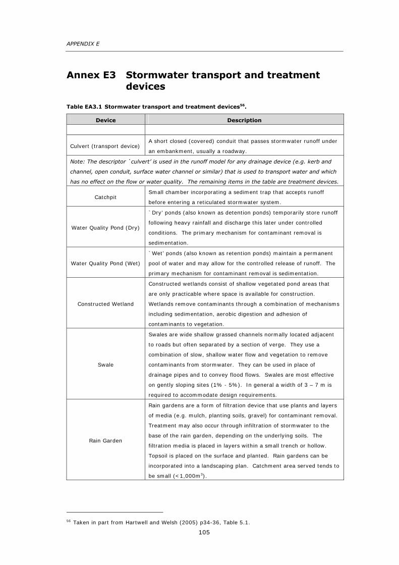
APPENDIX E
105
Annex E3 Stormwater transport and treatment devices
Table EA3.1 Stormwater transport and treatment devices56.
Device Description
Culvert (transport device) A short closed (covered) conduit that passes stormwater runoff under
an embankment, usually a roadway.
Note: The descriptor `culvert’ is used in the runoff model for any drainage device (e.g. kerb and
channel, open conduit, surface water channel or similar) that is used to transport water and which
has no effect on the flow or water quality. The remaining items in the table are treatment devices.
Catchpit Small chamber incorporating a sediment trap that accepts runoff
before entering a reticulated stormwater system.
Water Quality Pond (Dry)
`Dry’ ponds (also known as detention ponds) temporarily store runoff
following heavy rainfall and discharge this later under controlled
conditions. The primary mechanism for contaminant removal is
sedimentation.
Water Quality Pond (Wet)
`Wet’ ponds (also known as retention ponds) maintain a permanent
pool of water and may allow for the controlled release of runoff. The
primary mechanism for contaminant removal is sedimentation.
Constructed Wetland
Constructed wetlands consist of shallow vegetated pond areas that
are only practicable where space is available for construction.
Wetlands remove contaminants through a combination of mechanisms
including sedimentation, aerobic digestion and adhesion of
contaminants to vegetation.
Swale
Swales are wide shallow grassed channels normally located adjacent
to roads but often separated by a section of verge. They use a
combination of slow, shallow water flow and vegetation to remove
contaminants from stormwater. They can be used in place of
drainage pipes and to convey flood flows. Swales are most effective
on gently sloping sites (1% - 5%). In general a width of 3 – 7 m is
required to accommodate design requirements.
Rain Garden
Rain gardens are a form of filtration device that use plants and layers
of media (e.g. mulch, planting soils, gravel) for contaminant removal.
Treatment may also occur through infiltration of stormwater to the
base of the rain garden, depending on the underlying soils. The
filtration media is placed in layers within a small trench or hollow.
Topsoil is placed on the surface and planted. Rain gardens can be
incorporated into a landscaping plan. Catchment area served tends to
be small (<1,000m3).
56 Taken in part from Hartwell and Welsh (2005) p34-36, Table 5.1.
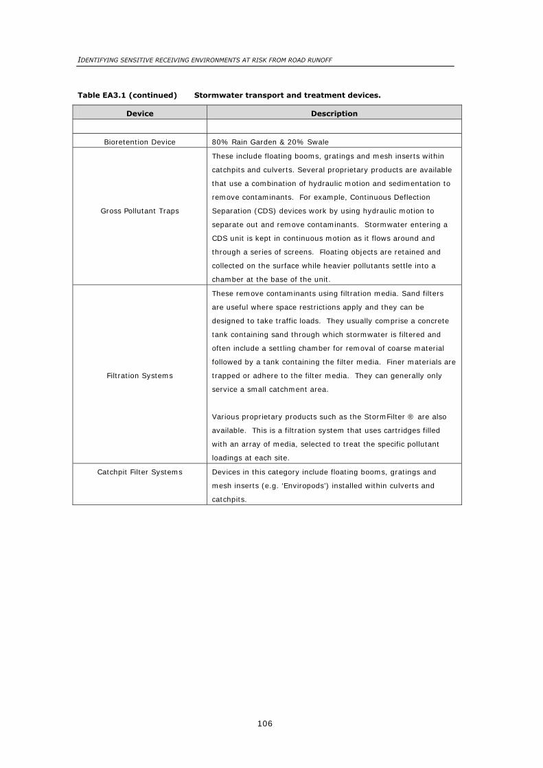
IDENTIFYING SENSITIVE RECEIVING ENVIRONMENTS AT RISK FROM ROAD RUNOFF
106
Table EA3.1 (continued) Stormwater transport and treatment devices.
Device Description
Bioretention Device 80% Rain Garden & 20% Swale
Gross Pollutant Traps
These include floating booms, gratings and mesh inserts within
catchpits and culverts. Several proprietary products are available
that use a combination of hydraulic motion and sedimentation to
remove contaminants. For example, Continuous Deflection
Separation (CDS) devices work by using hydraulic motion to
separate out and remove contaminants. Stormwater entering a
CDS unit is kept in continuous motion as it flows around and
through a series of screens. Floating objects are retained and
collected on the surface while heavier pollutants settle into a
chamber at the base of the unit.
Filtration Systems
These remove contaminants using filtration media. Sand filters
are useful where space restrictions apply and they can be
designed to take traffic loads. They usually comprise a concrete
tank containing sand through which stormwater is filtered and
often include a settling chamber for removal of coarse material
followed by a tank containing the filter media. Finer materials are
trapped or adhere to the filter media. They can generally only
service a small catchment area.
Various proprietary products such as the StormFilter ® are also
available. This is a filtration system that uses cartridges filled
with an array of media, selected to treat the specific pollutant
loadings at each site.
Catchpit Filter Systems Devices in this category include floating booms, gratings and
mesh inserts (e.g. ‘Enviropods’) installed within culverts and
catchpits.
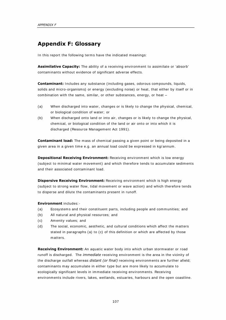
APPENDIX F
107
Appendix F: Glossary
In this report the following terms have the indicated meanings:
Assimilative Capacity: The ability of a receiving environment to assimilate or ‘absorb’
contaminants without evidence of significant adverse effects.
Contaminant: Includes any substance (including gases, odorous compounds, liquids,
solids and micro-organisms) or energy (excluding noise) or heat, that either by itself or in
combination with the same, similar, or other substances, energy, or heat –
(a) When discharged into water, changes or is likely to change the physical, chemical,
or biological condition of water; or
(b) When discharged onto land or into air, changes or is likely to change the physical,
chemical, or biological condition of the land or air onto or into which it is
discharged (Resource Management Act 1991).
Contaminant load: The mass of chemical passing a given point or being deposited in a
given area in a given time e.g. an annual load could be expressed in kg/annum.
Depositional Receiving Environment: Receiving environment which is low energy
(subject to minimal water movement) and which therefore tends to accumulate sediments
and their associated contaminant load.
Dispersive Receiving Environment: Receiving environment which is high energy
(subject to strong water flow, tidal movement or wave action) and which therefore tends
to disperse and dilute the contaminants present in runoff.
Environment includes:-
(a) Ecosystems and their constituent parts, including people and communities; and
(b) All natural and physical resources; and
(c) Amenity values; and
(d) The social, economic, aesthetic, and cultural conditions which affect the matters
stated in paragraphs (a) to (c) of this definition or which are affected by those
matters.
Receiving Environment: An aquatic water body into which urban stormwater or road
runoff is discharged. The immediate receiving environment is the area in the vicinity of
the discharge outfall whereas distant (or final) receiving environments are further afield;
contaminants may accumulate in either type but are more likely to accumulate to
ecologically significant levels in immediate receiving environments. Receiving
environments include rivers, lakes, wetlands, estuaries, harbours and the open coastline.

IDENTIFYING SENSITIVE RECEIVING ENVIRONMENTS AT RISK FROM ROAD RUNOFF
108
Sensitivity of Receiving Environment: The susceptibility or vulnerability of receiving
environments to adverse effects on ecology, human uses or human values (including
cultural values).