
Research 283 - Development of a New Zealand national ... · Booz Allen Hamilton (NZ) Ltd,...
78
Development of a New Zealand National Freight Matrix J. Bolland, D. Weir, M. Vincent Booz Allen Hamilton (NZ) Ltd, Wellington Land Transport New Zealand Research Report 283
Transcript of Research 283 - Development of a New Zealand national ... · Booz Allen Hamilton (NZ) Ltd,...

Development of a New ZealandNational Freight Matrix
J. Bolland, D. Weir, M. VincentBooz Allen Hamilton (NZ) Ltd, Wellington
Land Transport New Zealand Research Report 283

ISBN 0-478-25394-XISSN 1177-0600
© 2005, Land Transport New ZealandPO Box 2840, Waterloo Quay, Wellington, New ZealandTelephone 64 4 931 8700; Facsimile: 64 4 931 8701Email: [email protected]: www.landtransport.govt.nz
Bolland,* J., Weir, D., Vincent, M. 2005. Development of a New Zealandnational freight matrix. Land Transport New Zealand Research Report 283.110 pp.
Booz Allen Hamilton (NZ) Ltd, PO Box 10 926, Wellington, New Zealand.* now John Bolland Consulting, PO Box 51 058, Tawa, Wellington.
Keywords: commodity, EMME/2, freight, freight matrix, freight movement,freight transport, industry, loads, matrix, modelling, New Zealand, rail, road,transport

An important note for the reader
This report is the final stage of a project commissioned by Transfund New Zealand forthe 2003–2005 research programme, and is published by Land Transport New Zealand.
Land Transport New Zealand is a Crown entity established under the Land TransportNew Zealand Amendment Act 2004. The objective of Land Transport New Zealand is toallocate resources in a way that contributes to an integrated, safe, responsive andsustainable land transport system. Each year, Land Transport New Zealand invests aportion of its funds on research that contributes to this objective.
While this report is believed to be correct at the time of its preparation, Land TransportNew Zealand, and its employees and agents involved in its preparation and publication,cannot accept any liability for its contents or for any consequences arising from its use.People using the contents of the document, whether directly or indirectly, should applyand rely on their own skill and judgement. They should not rely on its contents inisolation from other sources of advice and information. If necessary, they should seekappropriate legal or other expert advice in relation to their own circumstances, and tothe use of this report.
The material contained in this report is the output of research and should not beconstrued in any way as policy adopted by Land Transport New Zealand but may beused in the formulation of future policy.

Acknowledgments
Booz Allen Hamilton (NZ) Ltd acknowledges the assistance provided for this researchproject by:
• Toll New Zealand Consolidated Ltd for assistance with details of rail freight
movements;
• Transport Engineering Research NZ (TERNZ) for background details of previous
research in the forestry field; and
• the many other businesses, organisations and individuals that provided details of
freight movements or other assistance, but which remain unnamed to protect the
confidentiality of those that have requested it.
5
Contents
Acknowledgments................................................................................................................4
Executive summary..............................................................................................................7
Abstract .............................................................................................................................10
1. Introduction .................................................................................................................111.1 Background ................................................................................................................111.2 Report structure..........................................................................................................11
2. Background ..................................................................................................................122.1 Context ..................................................................................................................122.2 The freight transport environment.................................................................................122.3 The freight transport industry .......................................................................................17
3. Overall approach to matrix development .....................................................................223.1 Introduction ...............................................................................................................223.2 Methodology...............................................................................................................223.3 Parameters.................................................................................................................23
4. Data collection .............................................................................................................284.1 Introduction ...............................................................................................................284.2 Key industries.............................................................................................................284.3 Market survey.............................................................................................................294.4 Supplementary data sources ........................................................................................32
5. Data analysis and the rail matrix .................................................................................345.1 Introduction ...............................................................................................................345.2 Survey returns............................................................................................................345.3 Supplementary industry analysis...................................................................................345.4 Commodity tables .......................................................................................................355.5 Road matrix inputs ......................................................................................................365.6 Rail matrix .................................................................................................................38
6. The road matrix and the final matrix ............................................................................416.1 Introduction ...............................................................................................................416.2 Process .....................................................................................................................416.3 Emme/2 overview .......................................................................................................416.4 Base network..............................................................................................................426.5 Data inputs ................................................................................................................426.6 Developing the seed matrix ..........................................................................................466.7 Developing the final road matrix ...................................................................................486.8 Sensitivity of average load ...........................................................................................576.9 Combining road with rail ..............................................................................................58
7. Examination of freight-trip-end model .........................................................................627.1 Introduction ...............................................................................................................627.2 Data used ..................................................................................................................627.3 Origin and Destination trip-end model estimation............................................................637.4 Application .................................................................................................................67
8. Conclusions ..................................................................................................................738.1 Main findings ..............................................................................................................738.2 Improvements to developing a freight matrix .................................................................748.3 Further work ..............................................................................................................75
Appendices
A References ................................................................................................................77B Industry by region ......................................................................................................79C Review of key industries and key firms .........................................................................83D Details of supplementary analysis ................................................................................93E Modelling technical notes ............................................................................................99

6
List of Tables
1.1 Population by region from 2001 census.......................................................................... 142.2 Industry by region (2002). .......................................................................................... 152.3 Imports by port for year ended 2003. ........................................................................... 162.4 Exports by port for year ended 2003. ........................................................................... 16
3.1 Freight growth rates at a GDP multiplier of 1.96. ............................................................ 243.2 Commodity groups sorted by share. .............................................................................. 253.3 Final commodity group descriptions. ............................................................................. 25
4.1 Summary of key industries and firms listed in Appendix C................................................ 29
5.1 Summary of 2002 tonnage data from the commodity tables. ............................................ 365.2 Inputs used to build the road freight matrix. .................................................................. 375.3 Total rail freight matrix. ............................................................................................... 40
6.1 Average heavy vehicle payload by region. ..................................................................... 456.2 Proportion of data by commodity and type. ................................................................... 476.3 Seed matrix for assignment-based estimation. ............................................................... 506.4 Seed, final and difference road matrix statistics. ............................................................ 526.5 Road final estimated matrix. ........................................................................................ 556.6 Road difference matrix of final minus seed. .................................................................... 566.7 Impact of load assumptions on final road matrix. ........................................................... 586.8 Road and rail matrix statistics. ..................................................................................... 596.9 Estimated road and rail freight matrix. .......................................................................... 61
7.1 Employment variables used for trip-end model examination. ............................................ 637.2 Estimated origin trip-end model coefficients. ................................................................. 657.3 Estimated destination trip-end model coefficients. .......................................................... 667.4 Trip-end-estimated total freight matrix. ......................................................................... 707.5 Absolute difference of fully-estimated minus trip-end-estimated freight matrix. .................. 717.6 Percentage difference (%) of fully-estimated minus trip-end-estimated freight matrix. ........ 72
List of Figures
2.1 Diagram of the general freight flows in New Zealand. ...................................................... 132.2 Estimated mode share by tonne-km (2002).................................................................... 182.3 Estimated mode share by tonnes carried (2002). ............................................................ 18
5.1 Distribution of trip length (km) of rail freight matrix. ....................................................... 39
6.1 Flow diagram showing the matrix estimation process. ..................................................... 436.2 Observed HV count locations. ....................................................................................... 446.3 Objective function value by iteration. ............................................................................ 496.4 Correlation of observed versus modelled road flows by iteration........................................ 496.5 Observed versus modelled (road seed matrix) assigned flows. .......................................... 516.6 Observed versus modelled (road final matrix) assigned flows. .......................................... 516.7 Trip length distribution of road seed matrix. .................................................................. 536.8 Trip length distribution of road final matrix..................................................................... 546.9 Trip length distribution of road difference matrix. ........................................................... 546.10 Assigned freight movements from road final matrix. ....................................................... 576.11 Trip length distribution of road + rail matrix. ................................................................. 59
7.1 Observed versus trip-end-estimated freight matrices by distance. .................................... 677.2 Scatterplot of fully-estimated versus trip-end-estimated regional freight movements. ......... 68

7
Executive summary
Introduction
This report documents the process and findings of a Land Transport New Zealand research
study carried out between 2003 and 2005.
The study objective was to:
• develop estimates of the main (non-urban) freight movements within New Zealand, by
commodity, tonnage, mode and origin-destination;
• relate these movements to the location of processing/export facilities in the case of
primary flows, and
• relate them to population and industrial production in the case of manufactured and
consumer goods.
In particular, the focus was on:
• longer-distance and higher tonnage movements; and on
• existing movements, rather than forecasts of future freight movements.
Freight transportation is one of the key but often overlooked areas of transport policy. Policy
decisions made by government can have a substantial impact on the movement of freight.
However, the requirements, patterns and complexities of the freight market are not well
understood and the management of these is often left to industry to resolve. The lack of
information has made it difficult to estimate impacts of policy changes and to understand and
plan for freight movements to, from and within the regions.
This study aims to begin the process of filling the information void. It provides the reader with
a broad overview of the types of freight transported, the methods used to move it, freight
origins and destinations, and establishes a basis for further more detailed research into this
topic. The focus is on the land transport modes of road and rail, with some investigation of
coastal shipping (excluding inter-island ferries). The study commences with an overview of the
freight transport environment and industry, and then describes the matrix and the
methodology used to build it.
Overall approach to development of a freight matrix
The overall approach taken to develop the matrix of long-distance higher tonnage freight
movements is outlined and the parameters around which it was constructed are summarised.
Data collection
The two elements to the collection of data used to build the initial road freight matrix are
detailed, and are:
• an initial research phase, which was used to identify key industries and firms and
provide a platform for further research, and
• a subsequent general data collection phase that utilised market surveys of freight
consignors or carriers, and other publicly available data sources to collect background
data.

DEVELOPMENT OF A NZ NATIONAL FREIGHT MATRIX
8
Data analysis and the rail matrix
The data collected, the analysis and classification procedures used are described, and details
are given of the inputs to the process of road matrix estimation and the final rail matrix. This
analysis involved the collation of data from all sources, standardisation to the base year (2002)
and to a common format, and the categorising of it by commodity and mode. Individual modes
were then separated, allowing the complete rail matrix to be constructed directly from the
available data, with rail bypassing the subsequent road matrix estimation process. Data
deficiencies precluded the creation of a final sea matrix and split by commodity.
The road matrix and final matrix
The development of the road matrix of freight movements is explained. Matrix estimation
formed the core part of the development of this matrix due to the limited range of road-based
data available. This process began with an initial matrix based on available industry data, then
used link-based data in the form of road traffic counts to update the initial matrix in an
iterative process until convergence was reached. Once completed, the road matrix was
combined with the rail matrix to give a total land transport matrix.
Freight-trip-end model
The development of a total freight-trip-end model is examined and compared with the total
matrix to check its suitability as a simplification of the previously applied matrix estimation
process. A trip-end model for freight origins/destinations takes the freight productions/
attractions estimated by the matrix estimation process and tries to relate these to explanatory
variables. This is simpler to implement than the full matrix approach, does not require detailed
data collection, and it gives the ability to crudely estimate future year matrices. The resulting
matrix is not as accurate as the fully estimated matrix.
Conclusions
Matrices of movements for the main land transport modes of road and rail are provided for the
2002 year, listing the approximate tonnages moving between and within origin and destination
regions. An indication of the significant commodities and industries utilising the freight
networks is also provided. This is the first time in New Zealand that such matrices have been
attempted or that inter-regional freight movement has been investigated in this detail.
The main findings are:
• Of the three main modes (road, rail, shipping), road transport conveys most freight
within New Zealand, having an approximate 83% share of tonnage and a 67% share of
tonne-km. Rail has an approximate 13% of tonnage and 18% of tonne-km, and coastal
shipping has a corresponding 4% of tonnage and 15% of tonne-km. Road has the
shortest average haul of the three main modes, while coastal shipping has the longest.
• Three regions –Auckland, Waikato and Bay of Plenty –account for the production and
attraction of over half of all road and rail freight, reflecting a concentration of population
and industry. Canterbury, the largest region by area, is the only other region with a
share of more than 10% of freight productions and attractions.

Executive summary
9
• Over two thirds of all road movements are of less than 200 km, with the Auckland region
dominating with around a quarter of both the production and attraction of all freight. The
greatest road tonnage corridors are, in descending order, Auckland to Auckland,
Canterbury to Canterbury, Waikato to Waikato, Bay of Plenty to Bay of Plenty, Waikato
to Auckland, and Waikato to Bay of Plenty. These corridors account for nearly half of all
road freight tonnage and show the preponderance of short-haul movements by road.
• Higher rail tonnages correspond to the locations of major industrial plants, mines and
ports. The greatest tonnage corridors for rail are, in descending order, Bay of Plenty to
Bay of Plenty, West Coast to Canterbury, and Waikato to Bay of Plenty. These three
corridors account for nearly half of all rail tonnage.
• A significant proportion (over half) of all freight cannot be easily classified into the
specific commodity groups as defined. This includes general freight movements, and
those relating to wholesale/retail, construction and other business sectors.
• The primary industries of agriculture and forestry are the largest originators of freight
that can be categorised into a specific commodity group. The transport of logs, milk and
livestock account for a significant share of total freight movements.
• A trip-end model for freight origins and destinations shows some correlation to the
modelled matrix, but further improvements in both the data and process would be
required to achieve a reasonable level of accuracy.
The results of this study have been limited by the availability of data and the associated
assumptions that have had to be made. The issue of commercial confidentiality reduced both
participation in the survey phase and the usefulness of the data supplied. This coupled with the
lack of statistics measuring freight and commodity data by weight have restricted the detail
that could be included. Additionally, the constantly evolving nature freight transport market
has limited the results presented here to a snapshot only of the economy as it was in 2002.
Nonetheless, the work is a considerable advance on anything available previously.
Improvements to developing a freight matrix
A number of recommended improvements could be made to the processes of developing the
freight matrix presented in this report, which would allow a more detailed matrix to be
developed and enhance the detail and results available.
For the full matrix such improvements would include:
• The compilation, by organisations such as Statistics New Zealand, of detailed statistics
relating to weight of goods transported. Where data is currently collected, it is often
recorded using measures other than weight, limiting its usefulness for tasks such as this.
• The collection of more complete observed data, by Transit New Zealand and other
organisations, such as the split of heavy vehicle types at telemetry sites.
• The use of better estimates of average loads, which would improve the accuracy of the
estimation process by limiting assumptions. The improvements to the collection of data
listed above might allow better estimates to be prepared.

DEVELOPMENT OF A NZ NATIONAL FREIGHT MATRIX
10
• For traffic counts, a review of the annualisation process to relate this more to the
movements of commercial vehicles. Average daily flows are currently designed primarily
to match general traffic patterns that are dominated by car journeys, and they may
therefore underestimate the weekday-oriented patterns associated with commercial
vehicles.
• Improvement of the modelled roading network and functions to take account of speed,
gradient, and road curvature, etc. This would allow a more accurate model of the
national transportation networks to be developed.
For the trip end approach such improvements would include:
• The collection of more disaggregated industry employment data for the trip-end model.
• The investigation of the feasibility of introducing factors to the matrix balancing process.
This would allow times or costs to be modified, to correct for inaccuracies in the network
or take account of perceptions and functions.
Further work
Three principal directions that future work might take are:
• The ongoing monitoring of the freight sector, which might involve the update of the
model every 2-3 years, to measure historical trends and increase knowledge of the
factors affecting the movement of freight in the New Zealand context.
• Use of the model to forecast future freight movements. This would be a valuable tool for
the planning of future requirements for roads, railways, ports and other freight facilities.
• The application of this process to create detailed freight matrices at the regional or even
TLA level. These would have a higher level of detail and could be combined as required
to look at freight movements within a specific geographic area (for example, the
southern South Island).
Abstract
Freight transportation is one of the key but often overlooked areas of transport
policy. Policy decisions made by government can have a substantial impact on the
movement of freight. However, the requirements, patterns and complexities of
the freight market are not well understood and the management of these is often
left to industry to resolve. The lack of information has made it difficult to estimate
impacts of policy changes and to understand and plan for freight movements to,
from and within the regions.
This study carried out between 2003 and 2005 aims to begin the process of filling
the information void. It provides the reader with a broad overview of what freight
is transported, where and how it is moved, and establishes a basis for further
more detailed research into this topic. The freight transport modes that are
studied are road, rail and to some extent coastal shipping.

1. Introduction
11
1. Introduction
1.1 Background
This report presents the findings of a research study undertaken as part of the Land
Transport New Zealand (formerly Transfund) 2004/05 Research Programme. The subject,
the Development of a National Freight Matrix, was initially part of the 2003/04 Research
Programme and was extended into the 2004/05 programme to allow completion.
As set out in Booz Allen Hamilton’s proposal of April 2003, the objective of the study was
to:
• develop estimates of the main (non-urban) freight movements within New Zealand,
by commodity, tonnage, mode and origin-destination;
• relate these movements to the location of processing/export facilities in the case of
primary flows, and relate them to population and industrial production in the case
of manufactured and consumer goods.
In particular, the focus was on:
• longer-distance and higher tonnage movements; and on
• existing movements, rather than forecasts of future freight movements.
1.2 Report structure
The report is structured as follows:
• Chapter 2 provides a background overview of the New Zealand freight transport
environment and industry.
• Chapter 3 presents an outline of the approach taken to developing the matrix and a
summary of matrix parameters.
• Chapter 4 details the collection of supporting data.
• Chapter 5 describes the analysis and classification of the data, and presents the rail
matrix.
• Chapter 6 explains the development of the road matrix, and presents this and the
final combined road and rail matrix.
• Chapter 7 examines whether an alternative freight trip end model can be
developed, and whether using such a model is a suitable simplification to the matrix
estimation process.
• Conclusions are reached in Chapter 8.

DEVELOPMENT OF A NZ NATIONAL FREIGHT MATRIX
12
2. Background
2.1 Context
Freight transportation is one of the key but often overlooked areas of transport policy.
Policy decisions made by government can have a substantial impact on the movement of
freight. However, the requirements, patterns and complexities of the freight market are
not well understood and the management of these is often left to industry to resolve.
Although earlier New Zealand studies have investigated various aspects of domestic policy
in this field, none have focused on the composition of long-distance (or local) freight
movements in terms of commodities moved, tonnages, origin-destination patterns and
mode shares, or investigated the relationships between them. The lack of information has
made it difficult for national policy makers to estimate the impacts of any policy changes
(pricing, regulation, etc.), and for regional planners to understand and plan for freight
movements to, from and within their regions.
This study aims to begin the process of filling the information void. It provides the reader
with a broad overview of what freight is transported, where and how it is moved, and
establishes a basis for further more detailed research into this topic. It commences with
an overview of the freight transport environment and industry.
2.2 The freight transport environment
The movement of freight within New Zealand is governed by several influencing factors,
which include both the country’s geography and various forces of supply and demand
(Cavana et al. 1997). These factors define the freight transport task by encouraging the
production and attraction of freight to specific locations, and affect the methods and
modes used to move it. The consequent links result in a complex network of transport
movements.
Geographically, the most important feature from a transport perspective is the
arrangement of New Zealand as two elongated main islands separated by a passage of
water (Cook Strait). As a consequence of this layout, each island has complete and self-
contained road and rail networks, linked with the other island via coastal shipping and
inter-island road and rail ferries to form a national network, and with the outside world
through gateways at international sea and to a lesser extent airports. Mountainous terrain
and the distribution of population dictate the course that the land transport networks
follow within each island.
Freight flows from points of supply within the system (origins), such as places of harvest
in rural areas or manufacturing plants, to points of demand (destinations), such as
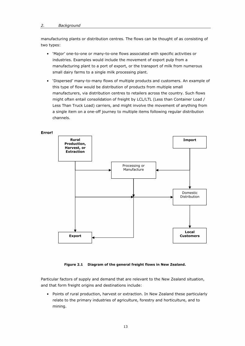
processing plants or export ports. Figure 2.1 illustrates the general freight flows within
the system. The actual flows can be highly complex and can involve many intermediate or
additional steps, involving trans-shipment, warehousing, or movement between multiple
2. Background
13
manufacturing plants or distribution centres. The flows can be thought of as consisting of
two types:
• ‘Major’ one-to-one or many-to-one flows associated with specific activities or
industries. Examples would include the movement of export pulp from a
manufacturing plant to a port of export, or the transport of milk from numerous
small dairy farms to a single milk processing plant.
• ‘Dispersed’ many-to-many flows of multiple products and customers. An example of
this type of flow would be distribution of products from multiple small
manufacturers, via distribution centres to retailers across the country. Such flows
might often entail consolidation of freight by LCL/LTL (Less than Container Load /
Less Than Truck Load) carriers, and might involve the movement of anything from
a single item on a one-off journey to multiple items following regular distribution
channels.
Error!
Figure 2.1 Diagram of the general freight flows in New Zealand.
Particular factors of supply and demand that are relevant to the New Zealand situation,
and that form freight origins and destinations include:
• Points of rural production, harvest or extraction. In New Zealand these particularly
relate to the primary industries of agriculture, forestry and horticulture, and to
mining.
Processing orManufacture
Import
DomesticDistribution
Export
RuralProduction,Harvest, orExtraction
LocalCustomers

DEVELOPMENT OF A NZ NATIONAL FREIGHT MATRIX
14
• The location and size of manufacturing and processing plants and the inputs that
they require for production. These range from large processing plants such as
Fonterra's Whareroa production facility near Hawera, to those of secondary
industries that are not closely tied to local inputs.
• The distribution of population. Cavana et al. (1997) indicate that this is an
important determinant of demand and, as a result, that it also influences the design
of logistics and distribution channels, particularly those relating to the service
industry. In the New Zealand context, population is not evenly distributed, with the
northern North Island dominating in both population and industrial activity. Much of
the warehousing and secondary industry is accordingly clustered around the
Auckland region, resulting in consumer-related distribution flows that operate in a
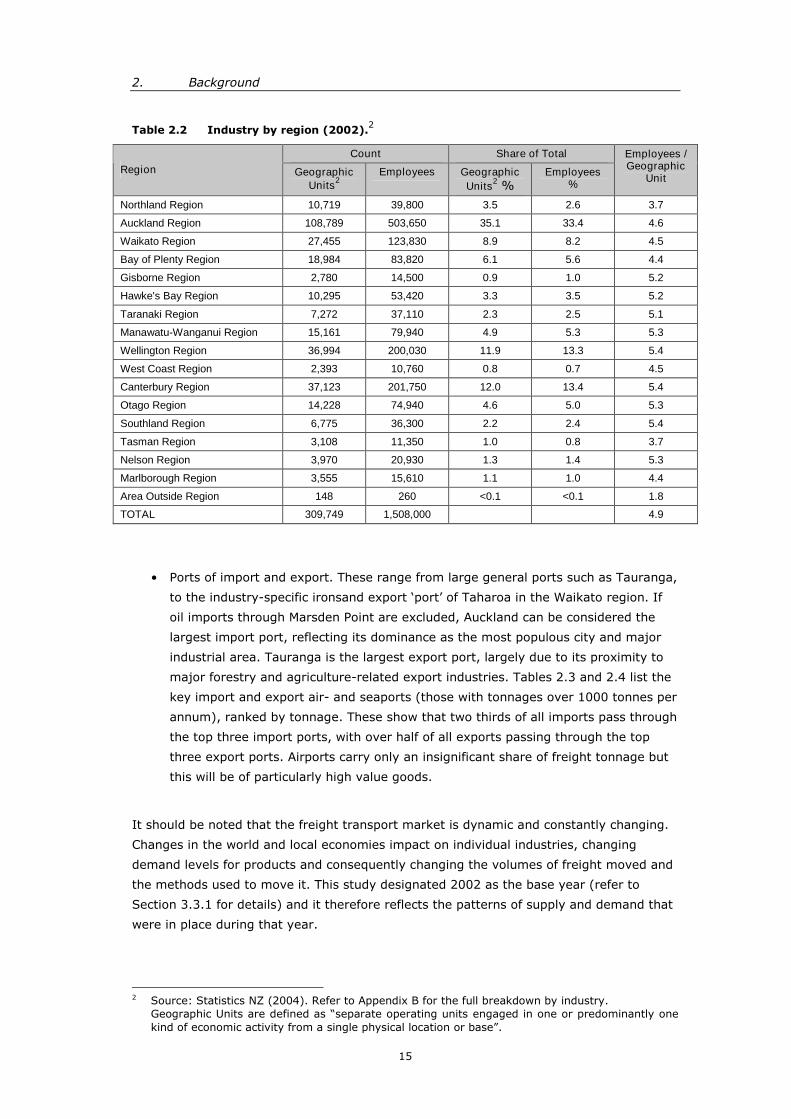
predominantly north-south direction. Table 2.1 shows the breakdown of population
by region from the 2001 census. Table 2.2 summarises industrial activity from
Appendix B, which lists the number of geographic units and employees in each
region that were involved in broad industry groups in the 2002 year.
Table 2.1 Population by region from 2001 census.1
Region Population Share of NationalTotal (%)
Northland Region 140,133 3.7
Auckland Region 1,158,891 31.0
Waikato Region 357,729 9.6
Bay of Plenty Region 239,412 6.4
Gisborne Region 43,974 1.2
Hawke's Bay Region 142,950 3.8
Taranaki Region 102,858 2.8
Manawatu-Wanganui Region 220,089 5.9
Wellington Region 423,765 11.3
Tasman Region 41,352 1.1
Nelson Region 41,568 1.1
Marlborough Region 39,558 1.1
West Coast Region 30,303 0.8
Canterbury Region 481,431 12.9
Otago Region 181,542 4.9
Southland Region 91,005 2.4
Area Outside Region 726 < 0.1
TOTAL 3,737,286 100
1 Source: Statistics NZ (2004).
2. Background
15
Table 2.2 Industry by region (2002).2
Count Share of TotalRegion Geographic
Units2Employees Geographic
Units2 %Employees
%
Employees /Geographic
Unit
Northland Region 10,719 39,800 3.5 2.6 3.7
Auckland Region 108,789 503,650 35.1 33.4 4.6
Waikato Region 27,455 123,830 8.9 8.2 4.5
Bay of Plenty Region 18,984 83,820 6.1 5.6 4.4
Gisborne Region 2,780 14,500 0.9 1.0 5.2
Hawke's Bay Region 10,295 53,420 3.3 3.5 5.2
Taranaki Region 7,272 37,110 2.3 2.5 5.1
Manawatu-Wanganui Region 15,161 79,940 4.9 5.3 5.3
Wellington Region 36,994 200,030 11.9 13.3 5.4
West Coast Region 2,393 10,760 0.8 0.7 4.5
Canterbury Region 37,123 201,750 12.0 13.4 5.4
Otago Region 14,228 74,940 4.6 5.0 5.3
Southland Region 6,775 36,300 2.2 2.4 5.4
Tasman Region 3,108 11,350 1.0 0.8 3.7
Nelson Region 3,970 20,930 1.3 1.4 5.3
Marlborough Region 3,555 15,610 1.1 1.0 4.4
Area Outside Region 148 260 <0.1 <0.1 1.8
TOTAL 309,749 1,508,000 4.9
• Ports of import and export. These range from large general ports such as Tauranga,
to the industry-specific ironsand export ‘port’ of Taharoa in the Waikato region. If
oil imports through Marsden Point are excluded, Auckland can be considered the
largest import port, reflecting its dominance as the most populous city and major
industrial area. Tauranga is the largest export port, largely due to its proximity to
major forestry and agriculture-related export industries. Tables 2.3 and 2.4 list the
key import and export air- and seaports (those with tonnages over 1000 tonnes per
annum), ranked by tonnage. These show that two thirds of all imports pass through
the top three import ports, with over half of all exports passing through the top
three export ports. Airports carry only an insignificant share of freight tonnage but
this will be of particularly high value goods.
It should be noted that the freight transport market is dynamic and constantly changing.
Changes in the world and local economies impact on individual industries, changing
demand levels for products and consequently changing the volumes of freight moved and
the methods used to move it. This study designated 2002 as the base year (refer to
Section 3.3.1 for details) and it therefore reflects the patterns of supply and demand that
were in place during that year.
2 Source: Statistics NZ (2004). Refer to Appendix B for the full breakdown by industry.Geographic Units are defined as “separate operating units engaged in one or predominantly onekind of economic activity from a single physical location or base”.

DEVELOPMENT OF A NZ NATIONAL FREIGHT MATRIX
16
Table 2.3 Imports by port for year ended 2003.3
Port Gross Weight(tonnes)
% Share ofNational Total
Whangarei / Marsden Point 5,444,743 33.7
Auckland Seaport 3,630,303 22.5
Tauranga Seaport 1,863,903 11.5
Christchurch Seaport (Lyttelton) 1,268,541 7.9
Invercargill Seaport (Bluff) 1,048,066 6.5
Wellington Seaport 1,009,034 6.2
Napier 684,084 4.2
New Plymouth 442,061 2.7
Timaru 287,243 1.8
Dunedin (Port Chalmers) 263,728 1.6
Nelson 97,679 0.6
Auckland Airport 77,044 0.5
Westport 23,805 0.1
Christchurch Airport 9,416 0.1
Wellington Airport 1,467 < 0.1
TOTAL 16,151,117
Table 2.4 Exports by port for year ended 2003.3
Port Gross Weight(tonnes)
% Share ofNational Total
Tauranga Seaport 7,864,543 31.0
New Plymouth 3,236,578 12.8
Christchurch Seaport (Lyttelton) 2,978,857 11.8
Auckland Seaport 2,006,391 7.9
Napier 1,975,668 7.8
Whangarei / Marsden Point 1,678,995 6.6
Nelson 1,132,750 4.5
Dunedin (Port Chalmers) 1,063,654 4.2
Taharoa 743,492 2.9
Wellington Seaport 634,333 2.5
Gisborne 605,786 2.4
Invercargill Seaport (Bluff) 577,218 2.3
Timaru 385,331 1.5
Picton 282,079 1.1
Auckland Airport 75,326 0.3
NZ Various 40,904 0.2
Westport 28,859 0.1
Christchurch Airport 17,840 0.1
Wellington Airport 1,338 < 0.1
TOTAL 25,329,941
3 Source: Statistics NZ (2003a).

2. Background
17
2.3 The freight transport industry
To perform the freight transport task, New Zealand has a highly competitive long-distance
domestic freight transport industry. Services are provided by numerous single-mode and
multi-modal freight companies which include road-based (truck) operators, rail (part of a
multi-modal business that includes road and sea divisions), coastal shipping (provided by
both local and international shipping companies), pipelines, and air transport carriers,
with competition occurring between both operators and modes.
While many of the transport companies involved in the New Zealand industry confine
themselves to a particular mode or niche area of specialisation, the trend within the
industry, across all modes, is towards greater consolidation and the provision of a wider
range of service offerings. Most of the major freight providers thus offer a broad array of
additional logistics services, covering the entire supply chain and including such areas as
warehousing and international freight. The larger freight companies do not confine
themselves to one transport mode, but instead use multiple modes to take advantage of
the particular time/cost/capacity advantages that each alternative offers.
This report focuses on the three main freight transport modes in terms of tonne-km:
road, rail, and coastal shipping. Figure 2.2 indicates that these provide the majority (over
99%) of non-pipeline freight transportation. Pipelines are used primarily to move gas and
petroleum products; with the most important being the Marsden Point-Auckland
petroleum products pipeline (conveying one third of the Marsden Point oil refinery’s
output) and the Maui and NGC long-distance gas transmission pipelines. Air freight is
primarily used to carry time-sensitive or perishable products (Cavana et al. 1997),
reflecting its comparatively high cost and low capacity, and it therefore has only a minor
share of the freight tonnage carried and tonne-km travelled. Figure 2.3 indicates the
approximate share of tonnage carried by the respective modes.
The dynamic market for freight transportation described in Section 2.2, and intense
competition between transport industry participants, has led to a continuously changing
industry environment. Some of the more noteworthy changes that have occurred since
the 2002 base year include:
• The 2003 acquisition of the railway company Tranz Rail (following financial
difficulties) by an Australian logistics company Toll Holdings, and the subsequent
transfer of the track and associated infrastructure to government ownership.
• A number of amalgamations between other freight carriers, the biggest of which
was the 2003 consolidation of two of the largest transport companies, Mainfreight
and Owens Group.
• A reduction in the number of vessels employed on coastal routes by the main New
Zealand-based coastal shipping operators.

DEVELOPMENT OF A NZ NATIONAL FREIGHT MATRIX
18
Figure 2.2 Estimated mode share by tonne-km (2002).4
Road, 66.5%
Rail, 17.8%
Sea, 15.3% Air, 0.3%
Figure 2.3 Estimated mode share by tonnes carried (2002).5
Road, 83.1%
Rail, 12.6% Sea, 4.2%
2.3.1 Road transport
Road transport is the dominant freight transport mode, with an estimated 67% of the
total tonne-km moved (Figure 2.2). Many of the road movements that contribute to this
mode share are short distance local moves; however a substantial number are longer
distance movements that often compete directly against other modes utilising the 10,700
kilometres of the state highway network. The principal advantage of road stems from its
ability to serve customers directly, accessing and using the roading network as required.
Rail and coastal shipping do not serve most freight customers directly and must therefore
rely on road transport to ‘bridge’ freight to their networks.
The transport of freight by road has increased considerably over time, particularly since
the 1983 removal of restrictions that prevented road transport from operating in direct
competition with rail. A recent profile of the heavy vehicle fleet by TERNZ6 (2004)
estimated that 19,450 million road freight tonne-km were operated in 2003, based on the
collection of Road User Charges (RUC), which compared to RUC-based estimates of
13,134 million tonne-km in 1996 and 8,854 million tonne-km in 1990 (Cavana et al.
1997). The TERNZ estimate compares with the lower 2002 figures of 12,923 tonne-km
4Note: Intended as a guide only. Road and rail shares are based on the findings of this study,coastal shipping (sea) share is calculated from Ministry of Transport (2005a) and excludes inter-island ferry traffic, air share is extrapolated from Cavana et al. (1997).
5Note: Intended as a guide only. Road and rail shares are based on the findings of this study,coastal shipping (sea) share is calculated from Ministry of Transport (2005a) and excludes inter-island ferry traffic.
6 TERNZ: Transport Engineering Research NZ.

2. Background
19
calculated by this study, and 15,782 million tonne-km calculated (and used as an input
for this study) from the 1999 figures of the HVLP project7 by Transit NZ (2001). However
the RUC-based estimates are based on a number of assumptions and are susceptible to
inaccuracies associated with the correct purchase of RUCs.
The road tonne-km were operated by three component groups:
• public carriers, which sold transport services to the market;
• own-account or private carriers, which performed an ‘in-house’ task hauling their
owners’ freight; and
• contract carriers, which contracted services to the two previous groups.
The commercial road freight transport industry, consisting primarily of public and contract
carriers, operated approximately 30% of the heavy vehicles over four tonnes8 in 2003.
The balance of vehicles were owned and operated by groups not primarily involved in
road transport, such as tradespeople, contractors, local councils and manufacturers.
The commercial industry is characterised by a large number of small operators, with 80%
of firms having five or fewer employees or vehicles (Road Transport Forum NZ 2004),
which is comparable with the road industry in other similar countries such as Australia.
This characteristic has not varied considerably from pre-deregulation levels as an early
1970’s study by King (1971) showed that 87% of firms had five or fewer vehicles at that
time, although it should be noted that modern vehicles are larger (up to 44 tonnes) and
operate over longer distances than their 1970’s counterparts did. Many of the smaller
operators provide contract services to the bigger operators and larger transport firms
often make significant use of a contracted owner-driver base.
2.3.2 Rail transport
Rail is the second largest mode in terms of freight tonne-km moved, with an approximate
18% market share (Figure 2.2). Because of its cost structure, it tends to be more
competitive in the high tonnage and/or long distance freight markets and consequently
has a greater market share in those areas than in the short distance or lower tonnage
markets.
The New Zealand rail system covers a network of 3898 kilometres, stretching from Otiria
in Northland to Bluff in Southland. A main trunk line runs from Auckland to Invercargill via
Hamilton, Palmerston North, Wellington, Christchurch, and Dunedin, and most other
major towns are served by either secondary or branch lines. Inter-island road/rail ferries
between Wellington and Picton link the lines in each island.
7 The HVLP study (Heavy Vehicle Limits Project) contained a comprehensive investigation into thelevel of payload tonne-km for the 1999 year. It was selected for its ability to provide a tonne-kmbreakdown by region and commodity.
8 22,900 of the 82,700 vehicles over four tonnes (Road Transport Forum (RTF) 2004).

DEVELOPMENT OF A NZ NATIONAL FREIGHT MATRIX
20
In the base year of this study, 2002, the rail network was owned by one vertically-
integrated company –Tranz Rail –that also operated all freight services over the system.
This firm, then named New Zealand Rail, had been purchased from the government in
1993. In 2003, following a period of financial difficulty, a majority stake in Tranz Rail was
acquired by the Australian company Toll Holdings. As part of that transaction, ownership
of the rail infrastructure (such as track, signalling and related staff and assets) was
transferred back to government ownership in mid-2004 (to the New Zealand Railways
Corporation, now known as ONTRACK). Under the associated agreement, Tranz Rail, since
renamed Toll New Zealand, has exclusive rights to operate all freight services until 2070,
subject to the maintenance of minimum traffic levels.
Toll NZ, which has renamed its railway division Toll Rail, operated a fleet of 232
locomotives and 4048 wagons, and carried 14.8 million tonnes of freight equating to 3853
million tonne-km in 2003 (Tranz Rail 2003). In spite of the financial problems that led to
the recent ownership changes, rail tonne-km have grown markedly since deregulation and
later privatisation, moving from 2735 million net tonne-km in 1990 (Cavana et al. 1997)
to the current level.
Toll currently operates three main types of freight services that were previously
introduced as part of a strategic reorganisation by Tranz Rail in 2001:
● ‘ITP’ intermodal (container) trains;
● ‘Sprint’ trains aimed at freight forwarder business between the major cities; and
● ‘Bulk’ trains carrying bulk commodities such as coal, milk and logs.
A separate division, Toll Tranzlink (formerly Tranzlink). has a large road transport
component and provides distribution services utilising all modes, while another division,
The Interisland Line, operates the ferry services.
2.3.3 Coastal Shipping
Coastal shipping accounts for an approximate 15% share of total tonne-km moved
(Figure 2.2). It can be divided into three component groups: inter-island road and rail
ferry (not included in the estimate of mode share), private bulk shipping, and general
‘public’ coastal shipping. Excluding inter-island ferry traffic, this mode carried an
estimated 4.9 million tonnes in 2003 (calculated from Ministry of Transport 2005a),
equating to an approximate level of 3200 million tonne-km, a decline from the estimated
4800 million tonne-km handled in 1990 (Cavana et al. 1997).
Ferry services operate between the North and South Islands, linking the road and rail
networks principally between Wellington and Picton. The Interisland Line and its
predecessors have dominated this market, operating road and road/rail ferries between
Wellington and Picton for over 40 years. The company currently operates three vessels.
The main alternative, Strait Shipping, has operated between Wellington, Picton and
Nelson since 1992. It diversified into the passenger service market in 2003 and currently
operates two vessels.

2. Background
21
Petroleum products, cement, coal and gas are the key bulk products transported by
coastal shipping. Petroleum products, the most significant of these with over half of all
non-ferry tonnage, are distributed by Silver Fern Shipping using two dedicated vessels,
operating from the Marsden Point refinery to 10 regional port terminals. The vessels also
back-haul condensate from New Plymouth to Marsden Point. Cement is distributed to
regional distribution centres by three bulk vessels, one operated by Golden Bay Cement
from the Portland cement plant near Whangarei, and the other two by Holcim NZ from the
Westport cement plant. Coal is barged from the South Island West Coast to New
Plymouth, Lyttelton (to supplement rail transport), and to the cement plant at Portland.
Gas (LPG) is distributed by foreign vessels (that have replaced a previously dedicated
domestic vessel), which are hired as required to perform coastal distribution.
Pacifica Shipping is the main domestic provider of general coastal shipping freight
services and currently operates two vessels. It is supplemented by Strait Shipping. Both
companies face direct competition from international shipping lines, which compete for
containerised, break-bulk and odd-sized cargoes, and have an estimated 15% share of
the coastal shipping market (P. Nicholas, New Zealand Shipping Federation, personal
communication, July 23, 2004; verified by Ministry of Transport 2005a). This competition
is a consequence of the partial deregulation of the industry in 1995, which allowed
international vessels visiting the country to transport cargo between ports in competition
with the domestic shipping. Prior to that, coastal shipping had been restricted to domestic
operators following the international practice of cabotage. International vessels compete
primarily for north-south traffic, utilising spare capacity between the unloading of imports
in northern ports and the loading of exports in southern ports. Both Pacifica and Strait
Shipping reduced their services and the number of vessels operated to the current level in
2003, as a result of intense price competition from the international lines (R. Grout,
Pacifica Transport Group, personal communication, October 28, 2004).

DEVELOPMENT OF A NZ NATIONAL FREIGHT MATRIX
22
3. Overall approach to matrix development
3.1 Introduction
This chapter presents an outline of the overall approach taken to develop the matrix of
freight movements, and summarises the parameters around which it was constructed.
3.2 Methodology
The methodology was governed by the project’s objectives, which were to estimate the
main long-distance, higher tonnage freight movements, define these by commodity,
tonnage, mode, origin and destination, and to relate them to the location of processing/
export facilities and to population. Given the complexity and detail required, a ‘bottom–
up’ approach, based around the freight flows and factors of supply and demand discussed
in Chapter 2 was employed to research and build the matrix. This was seen as the most
accurate way of gaining the detail needed to replicate the freight transport system.
The process involved the following steps, which have also been used as a basis for the
structure of the remainder of this report:
• Establishment of parameters relating to the research required for construction of
the matrix. This included the definition of ‘long-distance’ and ‘higher tonnage’ in the
context of this study.
• Assessment of the key industries responsible for the production and attraction of
freight, to serve as a basis for the collection of data relating to ‘major’ freight flows.
This step was undertaken in parallel with the previous step.
• Collection of data through the market survey of freight consignors for ’major’ flows
and freight carriers for ‘dispersed’ flows (defined in Section2.2), to build a matrix
of movements with known origin, destination, tonnage, commodity and mode, that
could be used as a basis for the final matrix.
• Collection of data from other publicly available sources, to supplement the matrix
movements collected through the market surveys. This data could then be
processed to produce freight origins or destinations based on total production/
attraction of freight. Undertaken in parallel with the market survey step.
• Analysis and classification of all data collected, with separation by mode to allow a
rail matrix to be constructed and a matrix estimation process to be used to
estimate the balance of unknown road movements. An intended coastal shipping
matrix could not be completed.
• Development of the road matrix using the matrix estimation process. There was
always an expectation that this step would be required to build the road matrix,
given the high complexity and disaggregated nature of the road industry.

3. Overall approach to matrix development
23
Known road movements were utilised to develop a seed matrix, and other
information about origins and destinations was then used to build a final matrix.
• Assembly of the final total freight matrix based on the estimated road matrix and
known rail matrix.
• Examination of whether a total freight trip end model could be developed and
whether it would be a suitable simplification to the matrix estimation process.
3.3 Parameters
A number of parameters were defined at the start of the project. These related to the
base year for the study, the classification of commodities, spatial classification (of freight
origins and destinations), and other details relating to the transport movements. These
were developed in parallel with the initial research into industrial activity (Section 4.2).
3.3.1 Base year
2002 was set as the base year for the study. This was selected as the year offering the
greatest range of published statistical data, and was subsequently found to be the year
for which survey participants most commonly provided data. For the purposes of this
study, the ‘2002 year’ was defined as any twelve-month period ending during 2002,
reflecting the fact that some data related to the calendar year, while others related to
financial or statistical years ending in months other than December.
To match data from other years to the base year, the 2002 levels were estimated using a
freight growth index derived from Gross Domestic Product (GDP). This used constant
price (Real) GDP9 for the year ending June (selected as the mid-point of the year),
multiplied by a freight growth elasticity of 1.96. This figure was calculated from inter-
island freight growth for a 2003 ferry study (Booz Allen Hamilton 2003). It was supported
by a 2002 report by the NZ Institute of Economic Research (NZIER 2002), which indicated
that the average annual growth in Real GDP between 1988 and 2002 had been 2.3%
while corresponding average annual transport growth over the same period had been
4.5%. Table 3.1 shows the growth rates used to estimate freight growth for each year.
It should be noted that tonnages estimated using these rates are an approximation only
and might be inaccurate in a number of ways. The above freight growth multiplier is
higher than that used in some similar studies, for example TERNZ (2003) used a
multiplier closer to 1.5, and freight growth in years of high GDP growth may have been
overestimated as a result.
Additionally, growth was applied uniformly to all data irrespective of trends within
individual industries, so the growth in movements of some commodities might have been
either under- or overestimated as a result.
9 GDP sourced from the seasonally adjusted chain-volume series in 1995/96 prices published byStatistics New Zealand (2004).

DEVELOPMENT OF A NZ NATIONAL FREIGHT MATRIX
24
Table 3.1 Freight growth rates at a GDP multiplier of 1.96.
Year Ended (June) GDP Growth (%)9 Estimated FreightGrowth (%)
1995 5.1 9.9
1996 3.8 7.5
1997 3.5 6.8
1998 0.4 0.9
1999 1.4 2.7
2000 5.5 10.9
2001 1.9 3.8
2002 3.9 7.6
2003 4.1 8.0
2004 4.4 8.6
Finally, the assumption was that logistics networks had remained static for the purposes
of the study, and no account was taken of the changes to individual transport routes or
modes that may have occurred between the data source year and the 2002 base year.
3.3.2 Commodity groups
The classification of movements by commodity was one of the main objectives of this
project. It was originally envisaged that such information would be readily available
through the identification of freight flows, and that it would provide an extra dimension to
the final matrix by identifying key origin-destination (O-D) patterns for individual
commodities.
The New Zealand Harmonised Classification (NZHC) system, used by Statistics New
Zealand and the New Zealand Customs Service, was initially chosen for the classification
of commodity data. Its 98 ‘Chapters’ (categories) were expected to provide a good level
of detail. However the system was found to be unnecessarily complex for this purpose
and generally did not match directly with the high tonnage commodity groupings
identified (see Section 4.2). It was subsequently decided that a classification system with
a reduced number of groups would provide a clearer picture of the major commodities
moved, and a higher level system with a reduced number of categories (16) was created,
with the groups based upon the key commodities identified and those chosen for a similar
study by Austroads (2003) in Australia.
All freight movements were thus assigned to one of the sixteen groups, either to one of
fifteen main commodity-based groups or to an ‘Other’ group (all movements that could
not be allocated to one of the main groups). The ‘Other’ group embraced a diverse range
of freight movements, including (but not limited to) general freight, wholesale and retail
supply, furniture removal and construction movements. Table 3.2 lists the sixteen
commodity groups, ranked by their estimated share of total road net-tonne-km, while
Table 3.3 provides the final definition of each group. Appendix D gives additional details
of assumptions relating to some groups. It should be noted that the composition of the
groups changed slightly over the course of the study, reflecting the availability of data.

3. Overall approach to matrix development
25
Table 3.2 Commodity groups sorted by share.
Commodity Group Estimated Share of TotalRoad Tonne-km (%)
10
Other 60.8
Logs 11.7
Milk 6.6
Livestock 6.4
Sawn Timber 2.9
Oil Products 2.6
Fertiliser 2.1
Coal 1.9
Wood Products 1.5
Produce 1.1
Cement 1.0
Minerals 0.5
Wool 0.4
Dairy 0.2
Metals 0.2
Meat 0.1
Total 100
Table 3.3 Final commodity group descriptions.
Commodity Group Booz Allen Description
Other All freight movements not fitting into the main commodity groupslisted below
Logs Logs moving from points of harvest to processing plants andports of export (includes woodchips)
Milk Unprocessed bulk milk moving from farms to processing plants
Livestock Live sheep, lambs and cattle moving from farms to processingplants or export ports
Sawn Timber Sawn timber moving from sawmills to local consumption andports of export
Oil Products Refined petroleum products moving from the Marsden Pointrefinery to retail distribution
Fertiliser Fertiliser moving from manufacturing plants to local consumption
Coal Coal moving from mines to local consumption or export
Wood Products Pulp, paper and wood panel products moving from productionplants to local consumption / export ports
Produce Unprocessed fruit, vegetables and grains moving to points ofconsumption, export or processing
Cement Cement moving from manufacturing plants to local consumption
Minerals Non-coal minerals, principally lime or marble moving from pointsof extraction to manufacturing/distribution
Wool Wool moving from farms to wool scourers and then to points ofexport or manufacture
Dairy Processed milk products moving from processing plants toconsumption or export
Metals Steel and aluminium moving from manufacturing plants to localconsumption and export
Meat Beef, veal, lamb, mutton, pigmeat and poultry moving fromprocessing plants to local consumption and export
Note: Other studies, such as those sourced for tonne-km references may define commoditiesdifferently.
10 Extrapolated from Cavana et al. (1997) and Transit New Zealand (2001).

DEVELOPMENT OF A NZ NATIONAL FREIGHT MATRIX
26
It should be noted that, while information was gathered and classified by commodity
during the data collection and analysis phases, data gaps precluded the inclusion of a
breakdown by commodity in the matrix building process. As a result, the final completed
matrix does not classify movements by commodity as originally intended. This is
discussed further in Sections 5.4 and 6.6.
3.3.3 Spatial classification
The complexity of the final matrix was dependent on the spatial level at which data was to
be collected. The Territorial Local Authority (TLA) was selected as the best level to at
which to work, with two advantages: it enabled New Zealand to be divided into 74
localised zones (excluding the Chatham Islands), permitting intra-regional movements to
be tracked; and it allowed the use of statistical data already collected at TLA level by
Statistics New Zealand and other organisations. The larger cities (Auckland and
Wellington) were to be incorporated into the final matrix on a regional basis to reduce the
impact of their complex localised inter-TLA movements.
All freight origins and destinations were assigned to a TLA. Where data was supplied on a
regional or national basis, two principal methods were used to allocate the traffic to the
correct TLA or multiple TLAs. The preferred method was to assign origins or destinations
based on the statistics of some driver of supply or demand, such as the number of people
employed in a relevant industry (full-time equivalents), the capacity/location of ports, the
number of animals farmed, or the number of hectares planted within each TLA in the
region. Where this method could not be applied, supply or demand was assigned to the
largest town- or city-based TLA within a region (for example Christchurch in Canterbury),
on the assumption that business and population would concentrate economic activity in
that area.
All data were subsequently categorised and analysed at the TLA level, however final
details have been presented at a regional level, both for clarity and because of the data
confidentiality requirements described elsewhere in this report. All movements are thus
assigned to fourteen region-based zones in the final matrices, which are based on
regional government areas, and not to the previously identified 74 TLA-based zones.
3.3.4 Transport movements
The focus of the study was on long-distance, high tonnage transport movements, made
by the main modes as previously described. Standards relating to the definition of
distance, tonnage and mode were defined at an early stage to ensure that there would be
consistency in the collection and processing of data.
As indicated in Section 3.3.3 above, the TLA was selected as the spatial level at which
data were to be collected. This effectively defined ‘long-distance’ as any inter-TLA
movement, and ‘short-distance’ as any intra-TLA movement. The complication of the
variability in size between large (i.e. Southland) and small (i.e. Napier) TLAs was
disregarded to maintain consistency in the approach to data collection, as was the fact
that some inter-TLA movements would be localised and therefore not relevant to the
3. Overall approach to matrix development
27
study. To downplay these factors, the minimum threshold for inclusion in the study was
specified as inter-TLA movements of more than 50 km and this was communicated to
those approached during the survey stage (Section 4.3).
The standard unit of measurement was set as the net weight in tonnes per annum. High
tonnage movements were defined as those of more than 5000 tonnes per annum to
minimise the effect of irregular movements and encourage survey response. Where data
was supplied in greater detail, it was included to a minimum level of 100 tonnes per
annum to take advantage of availability. Where data was supplied or available in
measures other than in weight (for example the number of containers/pallets moved or
the volume in litres) it was converted to a weight in tonnes using a conversion factor
(such as the density of 0.8 kg per litre for petroleum fuel) to allow inclusion.
Rules were also created for the definition of the mode of transport. Movements by a
single mode were considered to be by a single vehicle/train/vessel for the entire journey
and not split into component movements.
Movements by multiple modes (multi-modal journeys), such as barge-truck or truck-rail,
were broken into their separate component movements where known.
Where the component movements were not known, it was assumed that inter-island
movements would not be transhipped, and that rail and ship traffic would move by these
modes for most or all of the journey (excluding local pickup/delivery), except in areas
further from railheads/ports where it was assumed that there was transhipment to road.
Where the mode of transport was not specified, the movement was assumed to be by
road unless data from rail and coastal shipping operators showed otherwise.

DEVELOPMENT OF A NZ NATIONAL FREIGHT MATRIX
28
4. Data collection
4.1 Introduction
This chapter details the collection of data used to build the matrix. There were two
elements to this step:
• an initial research phase, which was used to identify key industries and firms and
provide a platform for further research (Section 4.2); and
• a subsequent general data collection phase that utilised market surveys of freight
consignors or carriers (Section 4.3) and other publicly available data sources
(Section 4.4) to collect background data.
4.2 Key industries
Initial research into key industries was undertaken at an early stage, in parallel with the
development of matrix parameters. It was used to provide a platform for subsequent
research by identifying the major freight generating industries and the key freight flows
related to these (the ‘major’ flows in Section 2.2). This research allowed later research to
be targeted towards the most important long distance freight flows.
A review of key industries and firms was produced. While not intended to be
comprehensive, it identified major commodities using the country’s freight transport
system, estimated the annual road tonne-km (as a guide to total tonne-km) and national
production tonnage for each commodity where possible, and provided a profile of the
relevant industry and suggested key firms within it. Data was sourced from the Ministry of
Economic Development, Statistics New Zealand, the Ministry of Agriculture and Forestry
(MAF), and reports from a variety of other sources, and used to construct a list of
significant commodities or industries and provide an approximate ranking of these by
tonne-km carried. As expected given their dominance as exports, most of the high tonne-
km and/or tonnage groups related to the primary industries such as agriculture and
forestry, or to minerals such as coal. A copy of the industry review, with reference
sources, is included as Appendix C of this report and its key findings are summarised in
Table 4.1.
As described above, the commodity groups identified at this stage became the basis for
the direction of further industry-based research. All groups were subsequently
investigated in greater detail, although some such as the large ‘Sand, Rock, Gravel, etc.’
group were later excluded from the matrix because of the short-distance localised nature
of the associated freight movements. Other categories such as ‘Wholesale and Retail’
were included in the matrix, but these were incorporated into the ‘Other’ group, largely
because of the difficulty in identifying and quantifying most movements.

4. Data collection
29
Table 4.1 Summary of key industries and firms listed in Appendix C.
PreliminaryCommodity Group
Estimated 2002Road Tonne-km
(million)
Total IndustryProduction
(million tonnes)
Road Tonne-km/ Production
(distance in km)
Logs 1466 20.94 70
Milk 827 14.37 58
Livestock 804 N/A N/A
Sand, Rock, Gravel, etc. 705 31.01 23
Bulk Wood Products 545 7.10 77
Wholesale & Retail 539 N/A N/A
Construction/Materials 456 N/A N/A
Lime & Fertiliser 322 7.83 41
Liquid Fuels 322 N/A N/A
Coal 240 4.46 54
Horticulture 141 N/A N/A
Grain 59 N/A N/A
Wool 44 0.20 226
Dairy Products 29 1.71 17
Meat 16 1.05 15
Cement N/A 1.05 N/A
Gas Fuels (LPG) N/A 0.22 N/A
Steel N/A 0.20 N/A
Aluminium N/A 0.05 N/A
Note:
(1) N/A indicates that this information was not available.
(2) Road Tonne-km/Production serves as a rough approximation of average haul in km.This is a guide only, as it is based on estimated tonne-km and assumes that allproduction of each commodity is transported once by road. No allowance is madefor transport by other modes (rail, sea or air) or for inconsistent definitions of eachcommodity across data sources. It is particularly evident that this figure is higherthan expected for wool. Wool production has declined by approximately 20% sincethe 1994 year on which the tonne-km figures are based and accounting for thiswould reduce average haul to around 180 km. This is still higher than expected, soit may be that other wool-related movements are included in the tonne-kmestimate.
4.3 Market survey
The market survey followed on from the initial industry research, and was used to collect
a matrix of movements with known origin, destination, tonnage, commodity and mode.
These were intended to be used as the basis for the building of the complete freight
matrix as discussed in Chapters 5 and 6.
Two types of flow were identified (see Section 2.2):
● ‘major’ (one-to-one or many-to-one) flows associated with specific activities or
industries, and
● ‘dispersed’ many-to-many flows of multiple products and customers.
DEVELOPMENT OF A NZ NATIONAL FREIGHT MATRIX
30
At the beginning of the study it was envisaged that each type of flow would require a
different research approach. Information on the ‘major’ flows was to be obtained by
approaching freight consignors (or consignees where applicable) to obtain information on
their transport tasks, and information on ‘dispersed’ flows was to be obtained by
approaching the carriers. It was expected that the overlap between the two sources of
data would provide a level of cross-checking.
4.3.1 Freight consignors
The primary source for information on ‘major’ flows was the surveying of freight
consignors. The firms that had been identified by the initial research as important
consignors within each of the commodity groups (see Section 4.2 and Appendix C) were
approached by telephone and email and invited to contribute information on their freight
flows to the study.
Additional firms were contacted as they became identified as significant freight
consignors. Industry organisations, such as the New Zealand Forest Owners Association
(NZFOA), were also surveyed to provide additional sources of information, particularly for
industries where tonnages were estimated to be high but where industry disaggregation
made it difficult to identify dominant firms.
Organisations were asked to provide estimates of their principal annual freight
movements (both inbound and outbound) for the most recent available year (with 2002
or 2003 stated as preferences), including commodity, origin and destination, tonnage,
and transport mode or modes. A standard spreadsheet template was offered to provide
guidance as to the type and format of data required and to standardise the response. To
simplify the task and to concentrate on the longer distance higher tonnage movements,
survey participants were asked to only include journeys of over 50 km with annual
tonnages of over 5000 tonnes. These were given as guideline minimum thresholds for
inclusion in the study (refer to Section 3.3.4).
This stage was a significant undertaking. In excess of 70 companies and industry
organisations were contacted and invited to contribute data to the project. The response
was disappointing given the commitment of resources, although it was in line with the
anticipated response for a survey of this type. Of those approached 26 companies
provided full or partial details of their logistics operations, which represented a 38%
response rate. Another nine organisations, representing a further 13% of those contacted,
indicated that their freight movements would not be relevant to the study, either because
tonnages were minor or because movements were of a short-haul nature only. The
aggregate sector (of sand, gravel and rock) exemplified this situation, having short
distance (if high tonnage) movements related to the low value of the product.
The detail of freight movements for some commodity groups was able to be gathered to a
reasonably complete point at the survey stage. The Coal, Minerals, Cement, Fertilisers
and Metals groups were well covered, largely as a result of the limited number of
participants in these industries, but also due to the willingness of most to contribute to
4. Data collection
31
the study. An acceptable level of data was also gathered for the Meat, Oil Products, Logs,
Sawn Timber, Wood Products and Other categories, although most forestry related data
came from existing research rather than direct industry participation. The Livestock,
Wool, Milk, Dairy and Produce groups proved very difficult to research, having little or no
input from industry.
A number of critical issues appear to have limited the response from freight consignors.
Principal amongst these was the issue of commercial confidentiality, which was the most
common reason given for non-participation in the study. Confidentiality was also
requested by most commercial organisations that did choose to participate, and the
majority of the information was supplied only on the basis that it would be kept
confidential. This issue reflects the small size of the New Zealand economy and the
corresponding minimal number of participants in most industrial sectors. Another problem
was that many organisations did not retain records of freight weights or volumes, and as
a consequence were unable to provide more than a rough estimate of tonnages for this
study. Finally, the issue of industry disaggregation made it difficult to obtain information
for some commodity groups with expected high tonnages. The wool industry illustrated
this situation, having relatively high tonnages but many independent industry players and
no central industry organisation co-ordinating or recording activities.
4.3.2 Freight carriers
The primary source for information on ‘dispersed’ flows was the surveying of freight
carriers, with different approaches undertaken for each mode. It was originally intended
that only the land transport modes –road and rail –would be included in the study.
However, coastal shipping was later added in recognition of its 'strategic fit' and
significant market share, particularly in the areas of inter-island and bulk freight. The
other transport modes –air transport and pipeline –were excluded as discussed in
Section 2.3.
Road proved to be the most difficult mode for which to obtain data, a situation not
entirely unexpected given the dispersed nature of the road industry. The original
methodology had proposed that road transport operators would be surveyed in a similar
way to freight consignors, and it anticipated that a response rate of approximately 25-
30% by numbers and up to 50% by tonnage could be expected. An initial approach was
made to the Road Transport Forum,11 to gain their input and help in contacting and
surveying operators. They declined to participate, and indicated that they expected that
the fast-changing and competitive nature of the industry, along with concerns about
commercial confidentiality, would prevent a reliable response from road operators and
11 This organisation describes itself as “the authoritative voice of the road transport industry…..created as a national body in 1997 to responsibly promote and advance the interest of the road transport industry and its member road transport operators. Over 80 percent ofcommercial road transport operators in New Zealand are members……[and it] acts for everyoneinvolved in the industry: owner drivers, fleet operators, in-house road transport operators andsuppliers of goods and services to the road transport industry, regardless of size, location or typeof business” (Road Transport Forum 2005).

DEVELOPMENT OF A NZ NATIONAL FREIGHT MATRIX
32
limit accuracy. For these and other reasons, road transport surveys were not
subsequently undertaken, and data from other sources and a process of elimination were
instead used to provide information on road transport tonnages.
In contrast to the difficulties in obtaining road data, a full matrix of rail tonnage data for
the 2002 year was supplied by Toll Rail. This information was made available on condition
that certain aspects were kept confidential.
Coastal shipping data were obtained through the survey of operators and the local
shipping industry organisation, the New Zealand Shipping Federation. Inter-island ferries
were treated as extensions of the road and rail networks and disregarded to avoid the
double-counting of movements. As with the survey of freight consignors, response rates
were variable, with confidentiality again proving a considerable barrier. Good detail was
obtained on the transport of bulk products such as petroleum products, cement and coal,
but it proved more difficult to quantify general freight movements, particularly the details
and level of domestic freight carried by foreign vessels in relation to the issue of cabotage
and, as a result, it was not possible to build a final matrix of sea-based freight
movements. A recently published report by the Ministry of Transport (2005) has
investigated the effects of the cabotage issue in greater detail.
4.4 Supplementary data sources
Additional data were collected from sources other than through the survey of freight
consignors and carriers, and these are discussed in more detail below and listed in the
appendices. Most of this information was publicly available; and was used to supplement
survey data, enabling analysis of commodities where survey response from industry was
weak, not available, or not requested; or to allow the cross-checking of other data.
The supplementary data sources generally provided information on single trip ends, as
commodity tonnages either originating or terminating, which contrasted with the matrices
of origin-destination pairs supplied by the survey sourced data. Information in this form
was less useful than the full matrix movements, however it was still valuable to the
process and it allowed lists of vector inputs to be created in preparation for the matrix
estimation stage (discussed in Section 5.3).
A number of issues limited the usefulness of much of the available information. Many
sources classified data by region rather than by TLA, or did not break national data down
into smaller units at all. Further, the definition of ‘region’ often varied depending on the
source and purpose for which it had been collected (for example, forestry regions differ
from regional government regions). Similarly, most data were not available by weight
(tonnage), with much publicly available information commonly quoted in either financial
units (for example, sales in dollars) or units of area (for example, hectares in production).

4. Data collection
33
4.4.1 Production data
Production data were used to estimate approximate tonnages of primary products
produced by TLAs. They were obtained from a variety of government sources including
the Ministry of Economic Development, MAF, and Statistics New Zealand (for example,
Agriculture Statistics 2002 (Statistics NZ 2003b)); and was supplemented by data
sourced from industry organisations such as NZFOA, Meat and Wool Innovation Economic
Service, and the Livestock Improvement Corporation.
4.4.2 Export data
Export data were used to determine the tonnage and port of departure for exports, and in
some cases to quantify imports. Export data were obtained principally from Statistics New
Zealand’s database of exports and imports by port, but they were also supplemented with
MAF and port company information.
4.4.3 Industry data
Industry data were used to determine locations and production levels of manufacturing
plants and the origins and destinations of freight relating to these. In some cases they
enabled transport paths to be traced from source through to points of export or
consumption. Data were obtained from Statistics New Zealand (principally data relating to
industry within each TLA), from industry organisations such as those listed in
Section 4.4.1, and from other industry sources such as annual reports and commercial
web sites.
4.4.4 Other sources
Two studies were referenced for estimates of the freight task in tonne-km. The Heavy
Vehicle Limits Project (HVLP) report for Transit New Zealand (2001) estimated the 1999
road freight task by region and industry, in payload tonne-km; while the Freight
Transport Industry in New Zealand working paper, by Cavana et al. (1997), provided
1994/95 estimates for major commodities moved by truck in addition to other general
transport information. These were used to estimate commodity group and total
movements by road, and provide a cross-check of information gathered from other
sources.
Additional key sources included the Heavy Vehicle Movements in New Zealand report for
the Land Transport Safety Authority by TERNZ (2003) (which provided assessments of
heavy transport movements for some commodities) and various regional reports. TERNZ
also supplied background research data relating to forestry industry transport
movements.

DEVELOPMENT OF A NZ NATIONAL FREIGHT MATRIX
34
5. Data analysis and the rail matrix
5.1 Introduction
This chapter describes the data collected, the analysis and classification procedures used,
and provides details of the inputs to the road matrix estimation process and the final rail
matrix. The analysis process involved the collation of data from all sources,
standardisation to the base year and common format, and classification by commodity
and mode. Individual modes were then separated, allowing the rail matrix to be
calculated.
5.2 Survey returns
Survey returns were received in a variety of formats, with many containing incomplete or
aggregated data that were often in a form that was difficult to use. All were put into the
standard format listing commodity, origin, destination, tonnage and transport mode for
each movement specified. Any data gaps were filled where possible, using the processes
described in Section 3.3. Processed data was then added to a series of standard
commodity tables, as described in more detail in Section 5.4 below.
5.3 Supplementary industry analysis
Additional analysis, using data obtained from sources other than from the surveys, was
performed on a number of commodity groups in two situations. The first was where the
survey returns were not considered to have provided a satisfactory proportion of the total
estimated movements of a commodity. This applied to the Milk, Livestock, Produce, Wool
and Meat groups. The second situation was where the freight consignors within a
commodity group had not been approached during the survey phase, where sufficient
public and carrier data were deemed to be available to map freight movements without
directly approaching the industry concerned. This applied only to the forestry related
commodity groups of Logs, Sawn Timber, and Wood Products.
This analysis was primarily aimed at providing an estimate of bulk movements relating to
the first stage of the production process: from collection/harvest/production in rural areas
to the initial points of processing or manufacture, although it was also used to estimate
further stages of the logistics process for the Wool, Meat, Sawn Timber and Timber
Products groups. It was not possible to produce a full matrix of origin-destination
movements for each commodity using this approach; rather two separate lists were
generated, one listing the estimated originating tonnages by TLA and the other listing
estimated terminating tonnages by TLA. These origins and destinations were then added
as vectors into the matrix estimation process as described in Section 6.5.

5. Data analysis & the rail matrix
35
The processing of this data involved a series of steps and assumptions, which are detailed
for each group (where applicable) in Appendix D. The main stages were:
• Generation of TLA origin tonnages: a level of production was estimated for the
commodity within each TLA, either using some type of production per unit (for
example, production per hectare multiplied by hectares planted per TLA), or
alternatively by allocating a national or regional production total to each TLA (as
described in Section 3.3.3).
• Generation of TLA terminating or destination tonnages: a level of consumption was
estimated for the commodity within each TLA, based on local drivers of demand,
such as exports by port, industrial activity, or population. This was done by
calculating the difference between total originating tonnage (identified in the
previous stage) and total exports, then allocating this difference to each TLA
according to a measure of industrial activity or population (using the same methods
as above). Any local exports could then be re-added to give a total consumption for
each TLA.
• Correction for known matrix movements: any ‘actual’ known matrix movements
(i.e. full origin-destination movements) were subtracted from the TLA origin and
destination tonnages generated above. This gave the final lists of unallocated road
origins and destinations by TLA (since all rail and most sea movements were
known), which could then be added to the commodity tables.
5.4 Commodity tables
A summary table was created for each commodity group. Both matrix- and vector-based
movements were then added to the appropriate tables to create a summary database of
information collected from all sources. As data were added to the tables, origins and
destinations were assigned to the appropriate TLA (where this had not already been done)
and tonnages were aligned to the base year using the process described in Section 3.3.1.
Tonnages were then assigned to the appropriate mode to allow 2002 mode totals to be
generated for each commodity.
The road tonnages from the commodity tables were retained and used as inputs to the
matrix estimation process. Rail and sea tonnages supplied by freight consignors were
disregarded, and operator-supplied data, being deemed more accurate, was instead used
to provide information on the movements relating to these modes. Coastal shipping was
excluded from further consideration at this point because of a shortage of data and, as a
consequence, a final sea matrix was not constructed. Table 5.1 presents a summary by
commodity of the road and rail tonnages used to create freight matrices for these modes.
Table 5.2 provides additional detail for road only (these figures are a guide only and may
not tally due to numerical rounding).

DEVELOPMENT OF A NZ NATIONAL FREIGHT MATRIX
36
Table 5.1 Summary of 2002 tonnage data from the commodity tables.
Commodity Group Available RoadCommodity
Tonnage
(million tonnes)
Rail CommodityTonnage*
(million tonnes)
Total AvailableTonnage
(million tonnes)
Other 1.6 2.5 4.2
Logs 18.8 3.6 22.4
Milk 13.0 0.8 13.7
Livestock 1.1 0.0 1.1
Sawn Timber 3.8 0.1 3.8
Oil Products 1.5 0.0 1.5
Fertiliser 1.9 0.2 2.1
Coal 1.1 2.7 3.8
Wood Products 2.0 1.4 3.3
Produce 3.1 0.2 3.4
Cement 1.2 N/A 1.2
Minerals 0.4 0.1 0.6
Wool 0.3 0.2 0.5
Dairy N/A 1.0 1.0
Metals 0.3 0.3 0.6
Meat 1.0 0.5 1.5
Total 51.1 13.6 64.7
* Rail commodity tonnages are estimated only. They have been matched as closely aspossible to the Booz Allen commodity groups; however they should be used only as aguide, due to potential differences in definitions and classifications.
Table 5.1 should be viewed only as a summary of the data gathered and applied to build
the road and rail matrices. It is clear that, although all rail movements are known, only a
portion of road tonnages have been explained (50-60% based on the later matrix
estimation) even though nearly 51.1 million tonnes of freight movements were accounted
for during the research stage. Road tonne-km data and industry production data provide
an insight into those areas where there is a particular shortfall (see Section 5.5 below).
The issues of confidentiality, insufficient survey matrix data, and a lack of road link-
based/traffic count information at a commodity level precluded the further use of this
information at a commodity level. Further stages used commodity data only for reference
purposes and, as a result, the final completed matrices do not break movements down by
commodity as originally intended.
5.5 Road matrix inputs
Table 5.2 lists the inputs that were used to build the road freight matrix. Matrix and
vector tonnages sourced from the commodity tables served as direct inputs to the matrix
estimation process, while the tonne-km data was used to provide check totals to the
estimation process (refer to Chapter 6 for further detail).

5. Data analysis & the rail matrix
37
Table 5.2 Inputs used to build the road freight matrix.
Commodity Group Road MatrixTonnage
(million tonnes)
Road VectorTonnage
(million tonnes)
Total Matrix +Vector Tonnage
(million tonnes)
Estimated RoadTonne-km
(million)12
Other 1.64 0 1.64 7,614
Logs 0 18.80 18.80 1,466
Milk 0 12.95 12.95 827
Livestock 0.27 0.83 1.10 804
Sawn Timber 0 3.75 3.75 357
Oil Products 1.51 0 1.51 322
Fertiliser 1.89 0 1.89 262
Coal 1.12 0 1.12 240
Wood Products 0 1.96 1.96 187
Produce 0.25 2.89 3.14 141
Cement 1.23 0 1.23 123
Minerals 0.43 0 0.43 60
Wool 0 0.31 0.31 44
Dairy 0 0 0 29
Metals 0.29 0 0.29 29
Meat 0.15 0.85 0.99 16
Total Calculated 8.78 42.34 51.11 12,523
Total from HVLP 15,782
Note:
(1) Tonnage figures are based on the available data collected for this research. They therefore representonly partial data as explained in Section 5.4.
(2) Tonne-km are provided only to indicate the relative magnitude of the transport task for eachcommodity. They are not comparable with tonnage figures, because of the inconsistent definitions ofeach commodity across data sources.
A comparison of road tonnages for each group, with estimated road tonne-km and
industry production levels (Table 4.1), reveals those commodity groups with a deficiency
of road tonnage data. It is particularly apparent that only a small share of the total likely
tonnage for the large ‘Other’ group has been collected (as expected, given the diversity of
road freight traffic), although many of these movements might be over short distances
and not relevant to this study. Other groups that appear to require much greater detail
are the ‘Livestock’ and ‘Dairy’ groups. The remaining groups have been assessed to an
acceptable level, although tonnage estimates are dependent on estimated values and
associated assumptions.
There is a variance of approximately 20% between the total tonne-km figure extrapolated
from the HVLP total and that calculated from the sum of the commodity groups. This can
be explained by the use of more than one source for commodity group tonne-km and the
difference in commodity definitions used by each source, and also by the possible
variance between individual commodity growth rates and the overall freight growth rate
applied to the study as a whole (Section 3.3.1).
12 Extrapolated from Cavana et al. (1997) and Transit New Zealand (2001).

DEVELOPMENT OF A NZ NATIONAL FREIGHT MATRIX
38
5.6 Rail matrix
The completed rail matrix is shown in Table 5.3. This can be interpreted by reading origin
regions (producers) vertically and the corresponding destination regions (attractors)
horizontally. For example, 282,000 tonnes originates in Auckland and terminates in the
Bay of Plenty.
From the matrix, it is clear that a high proportion of rail tonnage is related to the
productions and attractions associated with the locations of major industrial plants, mines
and ports. This is to be expected, given that heavier train movements occur where
tonnage is higher and these usually relate to the locations of the above facilities.
Two corridors can be used as examples. From Manawatu-Wanganui the highest tonnage
destination is Taranaki, and this is the location of a major dairy processing plant that
serves as a terminating point for unit milk trains from the Manawatu area. The most
important destination for rail tonnage originating on the West Coast is Canterbury, the
location of the export port of Lyttelton which serves as a terminating point for unit coal
trains from the Buller and Grey districts on the West Coast.
Examining the final matrix in further detail shows that Bay of Plenty region with its large
port (Tauranga), major forestry-related industry and good rail links, is both the largest
producer (22% of total) and attractor (35% of total) of rail freight. Waikato (with large
agriculture and forestry industries) and the West Coast (with a significant coal mining
industry) are the next largest producers of rail freight, with 20% and 15% shares of the
total respectively. Canterbury is the only additional significant attractor of freight (above
10% share) with 23% of the total, most likely related to the previously mentioned coal
exports and its role as an important distribution centre. Somewhat surprisingly, intra-
regional movements are significant in most parts of the country, although it is likely that
most of these are moving over longer distances within each region.
Figure 5.1 provides a trip length distribution for the rail matrix, displaying the number of
freight tonnes moved within each distance band, with each 200 km range shown in a
separate colour for clarity. It can be compared with similar plots for the road (Figure 6.8)
and total matrices (Figure 6.11), and is shown in the same scale as these to allow
comparison. This distribution shows that rail has a fairly even spread of tonnage over
most distances, with a slight predominance towards mid-length journeys in the region of
200 km. Table 6.8 compares road and rail statistics and shows that the average trip
length for rail is approximately 250 km.

5. Data analysis & the rail matrix
39
Figure 5.1 Distribution of trip length (km) of rail freight matrix.

DEVELOPMENT OF A NZ NATIONAL FREIGHT MATRIX
40
Table 5.3 Total rail freight matrix (annual tonnes ‘000).
Nor
thla
nd
Auc
klan
d
Wai
kato
Bay
ofP
lent
y
Gis
born
e
Hawke’s Bay
Tar
anak
i
Man
awat
u-
Wan
ganu
i
Wel
lingt
on
Tas
man
Nel
son
Mar
lbor
ough
Wes
tCoa
st
Can
terb
ury
Ota
go
Sou
thla
nd
TO
TA
L
Northland 405 157 5 43 - 0 0 0 0 - 0 0 0 1 0 1 613
Auckland 82 44 17 282 0 25 27 49 81 - 6 15 1 282 29 10 949
Waikato 8 76 777 1,862 0 1 6 6 4 - 1 0 0 33 4 2 2,780
Bay of Plenty 1 487 43 2,338 0 4 11 6 27 - 0 2 0 29 4 2 2,955
Gisborne - 0 0 0 - 2 0 0 0 - 0 0 - 0 0 0 4
Hawke’s Bay 1 53 3 8 25 143 46 111 37 - 1 1 0 38 1 3 471
Taranaki 0 68 19 132 0 5 179 8 49 - 2 2 1 29 5 1 499
Manawatu-Wanganui 0 56 3 18 0 43 730 27 163 - 1 1 0 35 3 2 1,082
Wellington 1 21 1 11 0 11 4 70 73 - 1 5 1 17 4 1 221
Tasman - - - - - - - - - - - - - - - - -
Nelson 0 7 1 1 0 1 0 1 2 - 22 2 0 8 0 0 46
Marlborough 0 37 0 8 0 2 1 3 16 - 8 9 0 20 5 2 111
West Coast 0 1 0 1 0 0 0 0 1 - 0 0 14 2,011 9 0 2,038
Canterbury 1 138 38 35 0 8 22 77 34 - 16 15 12 371 254 83 1,107
Otago 0 28 2 3 0 2 4 8 7 - 1 3 0 95 48 31 232
Southland 0 15 4 3 0 6 4 4 4 - 0 1 1 173 189 103 506
TOTAL 500 1,189 912 4,746 27 252 1,034 371 497 - 59 55 31 3,142 556 242 13,613
From
To

6. The road matrix & the final matrix
41
6. The road matrix and the final matrix
6.1 Introduction
This chapter explains the development of the road freight matrix and its amalgamation
with the rail matrix to form a total freight matrix.
Matrix estimation formed the core part of the development of the road matrix. This
technique was used to relate matrix-based data (TLA to TLA freight movements) to link-
based data (highway road vehicle counts), which was then used to update the matrix in
an iterative process until a convergence criterion was reached. A similar approach was
used for the Commercial Transport Study (CTS) in Sydney (Transport & Population Data
Centre 2002)13.
The process took data inputs relating to production and attraction of freight at specific
locations, as outlined in previous sections. Where full information was given, no further
processing was required; however where data was incomplete, estimation processes filled
the gaps to give a best estimate of a road freight matrix. This first matrix (or ‘seed’
matrix) was then used as an input to further estimation processes which attempted to
match matrix information with flow-based information (Transit New Zealand vehicle count
data), with the output giving the best estimate matrix. Finally, the road freight matrix
was combined with the rail freight matrix, to give a total land-based freight matrix.
6.2 Process
Figure 6.1 outlines the road-freight matrix estimation process, with each number referring
to an associated section in the report.
6.3 Emme/2 overview
Emme/2, the transport modelling package used for the estimation process, was developed
by INRO Consultants of Canada. It has the ability to model road and public transport
services and the interaction between them, and is well placed as a transport modelling
tool at a strategic level. Emme/2-based models are currently used in Auckland (through
ART and APT14) and Wellington (through WTSM14). The matrix estimation process
primarily uses matrix addition, matrix balancing, network calculation, and assignment
routines of the package. Appendix E provides additional information on Emme/2 and its
capabilities.
13 The Commercial Transport Study (CTS) Trip Table Estimation Procedure provides 2002- and baseyear (1996)-estimates of trips by light commercial, rigid and articulated trucks between eachtravel zone in the Greater Metropolitan Region of Sydney, Australia (T&PDC 2002).
14 ART Auckland Regional Transport; APT Auckland Public Transport; WTSM Wellington TransportStrategic Model.

DEVELOPMENT OF A NZ NATIONAL FREIGHT MATRIX
42
6.4 Base network
The base New Zealand network used for the freight matrix estimation project was
developed in Emme/2 to model a number of aspects of the Surface Transport Costs &
Charges Study for the Ministry of Transport (2005b). The network itself encompassed
both the rail and the main highway networks, and consisted of approximately 275 zones,
800 nodes, and 2650 directional links. It also included 12 modes (10 being rail/bus based,
1 transfer, and 1 auto), although only the highway (auto) mode was used for this
particular road-only modelling task.
No supporting documentation was available for the model network, and so a series of
checks were undertaken to ensure that it was valid and had a reasonable representation
of routes and corresponding distances. Such checks are vital to any matrix estimation
process. As a result, link-based distances were adjusted to broadly match observed
distances as described in Appendix E. Note that the highway network did not include
volume delay functions, and as such congestion has not been modelled, although this was
not seen as a significant issue as most long-distance freight movements would be either
outside the hours of congestion or on highways where congestion was not an issue.
Gradient and road curvature were also not modelled.
Checks relating to connectivity of links and zones were also undertaken. Where two links
were used to represent one piece of road, one was removed so that all demand assigned
on a link during the assignment process would be comparable with the observed
information and not located on adjoining links.
Freight movements were provided at a TLA level (as described in Section 3.3) but the
zone system in the Emme/2 network provided greater detail. Since there was no basis on
which to disaggregate the TLA data further, a representative zone was selected within
each TLA and all movements were assumed as going from (or to) this zone. A network
attribute was also created to represent the region that a particular highway link fell within
and this attribute was used to add region-specific average loads for link-based heavy-
vehicle flow data (see Figure 6.1).
6.5 Data inputs
Data inputs took the form of two distinct types: matrix-based and link-based inputs. The
matrix-based information was used as a starting point (since this did not include all
operators and commodities), and the link-based information gave an independent and
more complete source with which to improve the starting point.
Matrix-based input information took the form of either a full matrix, where complete
origin/destination matrix data was available; or a vector form, where information on
origins and/or destinations was available but not in matrix form. Chapter 5 discussed
these inputs.

6. The road matrix & the final matrix
43
Figure 6.1 Flow diagram showing the matrix estimation process.
6.4, 6.5, 6.6, 6.7 –refer to Sections 6.4, 6.5, 6.6, 6.7
Gradient MethodApproach
Convert toFreight Flows
Add ObservedMatrices Commodity Matrices
6.5 Matrix Inputs
6.5 Vector Inputs6.6 Calibration ofGravity Model foreach Commodity
Distance Matrix
6.6 First EstimateMatrix (Seed)
6.7 Matrix Link-based Updating
6.4 Emme/2Network
6.6 Matrix Balancingfor each Commodity
Average TripLength of allMatrices
6.7 Final Matrix
Checks and Statistics
6.5 ObservedLink-BasedVehicle Flows

DEVELOPMENT OF A NZ NATIONAL FREIGHT MATRIX
44
Link-based traffic information, based on data collected at telemetry sites, was provided by
Transit New Zealand for the 2002 year. This gave average annual daily total flows at 12
directional and 67 non-directional link locations on the state highway network, and the
proportion of heavy vehicles (HVs) at each location. These were used to give average
annual daily heavy vehicle movements.
Figure 6.2 shows the observed HV count locations and their relative magnitude. It would
have been useful to have had this data disaggregated further, by vehicle size, to better
determine average tonnage estimates at these locations, but this detail was not available.
Data were available at some (but not at most) locations by direction, and analysis of the
links where the direction could be determined showed that the average split was around
50:50, indicating that the flows were fairly symmetrical. It was therefore assumed that
where the direction could not be determined, flow would be split evenly in both directions.
Figure 6.2 Observed HV count locations.
Representative links within the Emme/2 model were determined and observed flows read
in as one of the link attributes. Because flows were received as ‘average daily vehicles’
they were converted to annual tonnes to match the matrix. The converted annual tonnage
by link was saved in another attribute and calculated using the following formula:
Tonnes i, j, r = AADT i, j x AveLoad r x Annualisation
where:
Tonnesi,j,r: Annual tonnage for link ‘i,j’ within region ‘r’ (tonnes/year)
AADT i,j: Average Daily Traffic (HMV’s) for link ‘i,j’ (vehicles/day)
AveLoad r: Average load factor within region ‘r’ (tonnes/vehicle)
Annualisation: 365 (days) as traffic is average annual daily traffic (AADT)

6. The road matrix & the final matrix
45
Average load factors (Table 6.1) were determined using data from the Heavy Vehicle
Limits Project (Transit NZ 2001), which gave annual vehicle km and payload tonne-km by
region and vehicle type for 1999. This classified vehicles as A (articulated), B (B-train)
and R (rigid) types, and also included a category called ‘other vehicle’ which appeared to
relate to smaller commercial vehicles (having an average payload of 3.3 tonnes). The
average payload took account of both empty running and partly laden travel.
Table 6.1 Average heavy vehicle payload by region (tonnes).15
Region All Vehicles Excluding‘Other’
Midpoint
Northland 6.3 11.1 8.7
Auckland 5.5 11.0 8.2
Waikato 7.9 14.7 11.3
Bay of Plenty 7.9 14.8 11.4
Gisborne 7.4 13.9 10.7
Hawke’s Bay 6.4 11.6 9.0
Taranaki 7.3 12.9 10.1
Wanganui-Manawatu 6.7 11.8 9.2
Wellington 5.5 11.5 8.5
Nelson-Marlborough 6.1 11.1 8.6
Canterbury 6.4 11.7 9.0
West Coast 7.0 11.2 9.1
Otago 7.0 13.3 10.1
Southland 7.1 13.1 10.1
National Average 6.6 12.5 9.5
Comparing across regions, Waikato and the Bay of Plenty had the heaviest average
payload, while Auckland and Wellington had the lightest (when smaller vehicles were
included). The variation is probably related to the types of commodities carried in each
region, the proportion of larger commercial vehicles, and the proportion of empty or part-
laden travel.
The table shows that there is a large variation in average payload when the ‘other’
vehicles are included, as these dominate the vehicle-km and tonne-km statistics. For
some links in the network (such as the Auckland Harbour Bridge or Ngauranga Gorge),
smaller freight moves would be more significant. However they would generally form a
lower proportion of longer distance travel, the focus of this freight study. We understand
that there may be a breakdown of heavy vehicles at a more disaggregated level at
telemetry locations, but this information was not available for this study (although more
work could be undertaken using this information).
15 Source: Transit New Zealand (2001).

DEVELOPMENT OF A NZ NATIONAL FREIGHT MATRIX
46
In light of these difficulties, it was decided that a middle ground would be used as the
central case (the midpoint column), and that sensitivities on the other two assumptions
would also be provided (see Table 6.7). It happens that the resulting freight matrix is
very sensitive to this assumption, and further research or data gathering is recommended
to give a better distribution of commercial vehicle types at counting locations.
There are issues relating to the annualisation factor used, in that the average daily flows
are designed predominantly to match car travel patterns rather than heavy vehicle
patterns. With heavy vehicle traffic concentrated during the week rather than at the
weekend, the averaging process may underestimate the number of heavy vehicles using
the network. However there was no basis on which to determine whether this was
significant, or to re-estimate this effect, and the annualisation factor has been left as is.
This could be another area for further investigation.
6.6 Developing the seed matrix
The ‘seed’ matrix was the starting matrix whereby assigned network flows were matched
to observed network flows. It was created using road matrix data inputs described in
Sections 5.5 and 6.5, and represented the best initial matrix based on the available
information.
The process of estimating a best road freight matrix took a number of steps, using the
matrix and vector data inputs as a starting point. Table 6.2 outlines the proportion
supplied in either a matrix form (i.e. where the full journey was known), or in vector form
(where total outputs and inputs were known but the individual movements were not).
Overall, only 17% of the total tonnage supplied was in a matrix form and, consequently,
most of the starting or seed matrix had to be estimated.
The first part of the estimation process was to convert vector-based information to a
matrix form, with specific origin to destination flows. This was achieved by taking the row
and column totals (origin and destination vectors) and distributing trips between them
based on a distance function (to represent utility), to ensure an average trip length. An
entropy model was used for this purpose (described in Appendix E).
The usual approach is to change the scaling parameter in the model so that the average
trip length of the resulting matrix matches an observed or known total. Research into
average trip lengths for freight movements did not result in any data that could be
applied in this case (in total, let alone by commodity), and the only alternative was to
base average trip lengths on the commodity matrices supplied. These gave average trips
ranging from 62 km to 228 km. However, as the commodity matrices provided only a
small share of supplied tonnage (17% on average), the use of commodity-specific trip
lengths was deemed inappropriate, particularly since much of this information was
available for only one consignor and/or one region (and not representative of the national
situation), or not available at all.

6. The road matrix & the final matrix
47
Table 6.2 Proportion of data by commodity and type.
Commodity Matrix Proportion(%)
Vector Proportion(%)
Other 100 0
Logs 0 100
Milk 0 100
Livestock 24 76
Sawn Timber 0 100
Oil Products 100 0
Fertiliser 100 0
Coal 100 0
Wood Products 0 100
Produce 8 92
Cement 100 0
Minerals 100 0
Wool 0 100
Dairy No data No data
Metals 100 0
Meat 15 85
Share of total tonnage % 17 83
As a result, the average trip length of all commodities combined, 137.3 km, was selected
as the final average trip length. It should be noted that the use of commodity-specific trip
lengths would have made little difference to the resulting matrix in totality, as such
numbers would have changed only the allocation of tonne-km within individual
commodities. Additionally, the lack of commodity-related link-based (traffic-count)
information would have prevented estimation at a commodity level in any case.
Evidence suggested that trip lengths for the Produce group were significantly shorter than
the average of 137.3 km. For this reason, a much lower trip length of 69 km was
assumed for this group, based on the existing matrix information. Since Produce data was
available only at the origin end, a singly constrained balancing approach (used in
situations where one trip end is unknown) was used to allocate trips.
Emme/2 has a matrix balancing function within the modelling suite to ensure that row
and column totals are in balance. It is an iterative approach, which stops when the
maximum percentage change in balancing coefficients is within a certain tolerance. A
series of balancing factors are determined for each origin and destination zone so that,
multiplied with the entropy matrix, the row and column totals match the origin and
destination vectors. The sum of the balanced matrices and the full supplied matrices
forms the ‘seed’ matrix to be used in the assignment-based matrix re-estimation. This
matrix is somewhat representative of relative freight movements. However it reflects data
availability, so it is not a true representation of actual freight movements.

DEVELOPMENT OF A NZ NATIONAL FREIGHT MATRIX
48
The seed matrix (Table 6.3) distributes the 51.1 million tonnes (see Table 5.2), with
approximately 50% of tonnage within region. It mirrors the greater availability of
information relating to rural industries, and so does not provide a true representation of
actual movements. It indicates that the largest generator of freight is the Waikato region,
which is shown as having around a third of all freight production. This is followed by
Canterbury, with around 10% of the total. Waikato is also shown to be the largest freight
destination, attracting almost a quarter of the total, and this is followed by Bay of Plenty
with close to 20% of the total, probably related to the large port at Tauranga. Other
notable destinations include Auckland and Canterbury with around 9% each. Auckland is
not dominant in the seed matrix however, and it is likely that this is because of a lack of
information about industries that prevail in that region, such as secondary manufacturing
and distribution.
6.7 Developing the final road matrix
The seed matrix was used as an input to a link-based form of matrix estimation.
Observed freight tonnages by link were loaded onto the highway network. The starting
matrix was then assigned on the network and assigned link flows compared with the
observed, with the difference computed. A gradient matrix was then determined, and
used to adjust the freight matrix in the right direction based on the largest discrepancy,
so as to minimise the total impact on the seed matrix. This routine was repeated until the
correlation of observed to modelled after assignment was high (50 iterations). Since the
factors are multiplicative, and the updating process only changes cells that have a value
other than zero, each zero-cell was given a minimum value of 0.001 to allow trips to be
generated where required (a standard procedure in matrix estimation).
Figures 6.3 and 6.4 show the convergence of the process. The objective function in
Figure 6.3 is related to the sum-of-squares of the difference between observed and
modelled between iterations, with the difference reducing as the number of iterations
increases. Similarly, the correlation plot of observed versus modelled flows in Figure 6.4
shows how well the assigned matrix fits the link-based tonnages and this indicates a
significant improvement through the process. Initially the fit of observed versus modelled
flows was not particularly good at around 0.2 (Figure 6.5).
This was driven by some significant outliers, particularly over the Auckland Harbour
Bridge where the seed matrix did not include some of the shorter freight journeys that
occur within the Auckland suburban boundary. Subsequent iterations improved the
correlation measure to be significantly closer to ‘1’ (a perfect match), so that after 15
iterations the modified matrix explained 90% of the observed variation, and that at 50
iterations it approached 99% with no significant outliers (Figure 6.6).

6. The road matrix & the final matrix
49
Figure 6.3 Objective function value by iteration.
0
100000
200000
300000
400000
500000
600000
0 5 10 15 20 25 30 35 40 45 50
Iteration
Ob
ject
ive
Fu
nct
ion
Figure 6.4 Correlation of observed versus modelled road flows by iteration.
0
0.1
0.2
0.3
0.4
0.5
0.6
0.7
0.8
0.9
1
0 5 10 15 20 25 30 35 40 45 50
Iteration
R^
2O
bse
rved
vsM
od
elle
d

DEVELOPMENT OF A NZ NATIONAL FREIGHT MATRIX
50
Table 6.3 Seed matrix for assignment-based estimation (annual tonnes ‘000).
Nor
thla
nd
Auc
klan
d
Wai
kato
Bay
ofP
lent
y
Gis
born
e
Hawke’s Bay
Tar
anak
i
Man
awat
u-
Wan
ganu
i
Wel
lingt
on
Tas
man
Nel
son
Mar
lbor
ough
Wes
tCoa
st
Can
terb
ury
Ota
go
Sou
thla
nd
TO
TA
L
Northland 1,822 733 154 64 1 2 12 3 0 0 0 0 0 0 0 0 2,790
Auckland 398 1,263 680 234 6 24 24 44 33 0 0 0 0 6 0 0 2,713
Waikato 590 1,639 7,908 4,777 164 786 477 416 98 9 12 16 1 5 0 0 16,898
Bay of Plenty 64 531 1,536 2,262 44 75 87 100 13 0 0 1 0 0 0 0 4,714
Gisborne 10 15 127 461 520 210 4 19 11 1 1 1 0 0 0 0 1,380
Hawke’s Bay 43 82 411 426 227 1,396 71 371 127 4 5 7 1 3 1 0 3,174
Taranaki 32 122 336 136 4 31 1,454 174 26 1 1 1 0 0 0 0 2,319
Manawatu-Wanganui 23 81 332 238 17 214 406 662 237 8 9 14 1 6 0 0 2,248
Wellington 3 9 57 39 7 89 143 424 615 16 34 41 2 14 1 0 1,493
Tasman 1 1 12 7 1 9 32 36 134 766 702 127 51 44 7 0 1,930
Nelson 0 0 1 1 0 1 0 2 31 63 111 67 36 15 4 0 334
Marlborough 1 1 20 15 2 18 36 50 196 131 188 281 25 65 1 0 1,030
West Coast 0 1 7 2 0 1 31 25 22 55 47 42 359 166 21 2 779
Canterbury 1 5 21 8 1 4 84 76 36 87 115 156 256 3,854 290 85 5,078
Otago 0 0 0 0 0 0 1 1 1 2 2 2 8 319 1,053 631 2,021
Southland 0 0 0 0 0 0 2 1 0 2 1 1 19 198 488 1,508 2,221
TOTAL 2,988 4,483 11,601 8,670 995 2,861 2,863 2,404 1,581 1,145 1,230 757 760 4,693 1,865 2,226 51,123
From
To
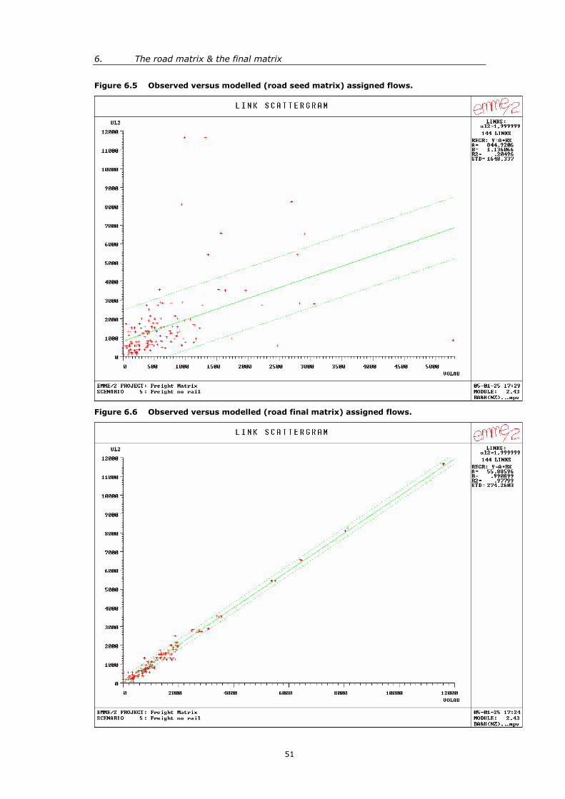
6. The road matrix & the final matrix
51
Figure 6.5 Observed versus modelled (road seed matrix) assigned flows.
Figure 6.6 Observed versus modelled (road final matrix) assigned flows.

DEVELOPMENT OF A NZ NATIONAL FREIGHT MATRIX
52
The resulting final road matrix after 50 iterations is much larger than the seed, by around
75% in volume and 90% in tonne-km. Freight volumes not explained by the seed matrix
have a longer average trip length than the seed (158 km v 133 km), which in turn
increases the average trip length of the final matrix to 144 km. While there are no
corresponding observed volumes to compare against, tonne-km estimates from the HVLP
study (Transit New Zealand 2001) gave a total of 12.8 billion (bn) tonne-km across all
vehicles for 1999. This compares well with our 2002 estimate of 12.9 bn tonne-km. It is
difficult to identify exactly how the freight market has changed since 1999, but with
freight movements somewhat correlated with GDP, we would expect them to be higher in
the 2002 year of our matrix. Using the growth estimates discussed in Section 3.3.1 and
the 1999 HVLP figures, the total tonne-km level could be as high as 15.8 bn tonne-km. As
such, our estimate may well be on the conservative side, accounting for 82% of tonne-km
by this measure (12.9 bn v 15.8 bn tonne-km), but it is clearly in the right order of
magnitude. It should be noted that this study and the HVLP have reached these figures in
an independent way.
As a further check, the tonne-km were divided by the average load factor to give vehicle-
km, and compared with the HVLP. The 12.9 bn tonne-km equates to approximately
1.36 bn vehicle-km (VKM) (using the national average load factor of 9.5 under the
midpoint scenario, see Table 6.1), while the HVLP study gave the total nationwide vehicle-
km as 0.69 bn VKM for A, B and R type vehicles,16 and 1.24 bn VKM for other smaller
commercial vehicles. In constructing our matrix we used a weighting of ½ for the smaller
commercial vehicles (to give the average payload), so weighting the smaller commercial
vehicles by ½ gave a nationwide vehicle-km value of 1.32 bn VKM (0.69+0.5×1.24). This
is around 3% lower than our value, and the difference can be partially explained by a
difference in base year, but it does indicate that the matrix is broadly consistent with
other information.
Table 6.4 Seed, final and difference road matrix statistics.
Matrix Tonnage (million) Tonne-km (million) Ave Trip Length
Seed 51.1 6818 133.4
Difference 38.5 6105 158.5
Total 89.6 12923 144.2
Seed 57% 53%
Difference 43% 47%
Table 6.4 presents summary statistics of the seed, final and difference (between the seed
and final) road matrices. The actual final road matrix is shown in Table 6.5 and the
difference matrix is shown in Table 6.6. Figures 6.7 to 6.9 display the number of freight
tonnes moved within each distance band of each matrix.
16 A –Articulated; B –B-train; R –rigid vehicles.

6. The road matrix & the final matrix
53
Examining the final road matrix (Table 6.5) in detail shows that the Auckland region is a
significantly larger player in both the production (23% of total) and attraction (25% of
total) of freight movements than in the seed matrix. This reflects the dominant role of
that city noted in Chapter 2. Waikato (contributing 20% of productions and 16% of
attractions) and Canterbury (13% productions and 12% attractions) are still very
important, and Bay of Plenty also remains as both a strong producer and attractor of road
freight. Intra-regional freight movements now comprise around 55% of the total (rather
than 50% in the seed matrix), indicating a higher proportion of shorter distance trips.
The seed matrix (the distribution for which is shown in Figure 6.7) contains around 75%
of freight movements within 200 km, and a further 15% between 200 km and 400 km. In
comparison, the final matrix (the distribution for which is shown in Figure 6.8) has a lower
proportion of trips of less than 200 km (around 73%) and a higher proportion between
200 km and 400 km (around 20%). This indicates the matrix estimation process
increased the proportion of medium and longer distance movements at the expense of
shorter distance movements. The difference-matrix trip-length distribution (Figure 6.9)
shows shorter distance (less than 200 km) freight movements comprise around 68% of
the total, while medium length (200-400 km) movements comprise around 24%.
Figure 6.7 Trip length distribution of road seed matrix.

DEVELOPMENT OF A NZ NATIONAL FREIGHT MATRIX
54
Figure 6.8 Trip length distribution of road final matrix.
Figure 6.9 Trip length distribution of road difference matrix.
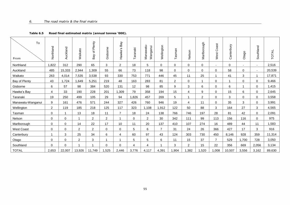
6. The road matrix & the final matrix
55
Table 6.5 Road final estimated matrix (annual tonnes ‘000).
Nor
thla
nd
Auc
klan
d
Wai
kato
Bay
ofP
lent
y
Gis
born
e
Hawke’s Bay
Tar
anak
i
Man
awat
u-
Wan
ganu
i
Wel
lingt
on
Tas
man
Nel
son
Mar
lbor
ough
Wes
tCoa
st
Can
terb
ury
Ota
go
Sou
thla
nd
TO
TA
L
Northland 1,822 312 290 65 3 2 18 5 0 0 0 0 - 0 - - 2,516
Auckland 485 15,333 2,944 1,309 55 66 73 118 98 0 0 0 0 58 0 - 20,539
Waikato 263 4,014 7,535 3,538 93 330 753 771 446 45 11 25 1 41 3 1 17,871
Bay of Plenty 43 1,724 1,649 5,251 219 48 163 283 81 2 0 1 0 1 0 0 9,466
Gisborne 6 57 98 384 520 131 12 98 85 9 3 6 0 6 1 0 1,415
Hawke’s Bay 4 33 190 228 201 1,309 79 358 194 15 4 9 0 15 6 0 2,645
Taranaki 19 250 499 105 29 94 1,826 457 269 5 1 2 0 3 0 0 3,558
Manawatu-Wanganui 9 161 476 571 244 327 426 760 946 19 4 11 0 35 3 0 3,991
Wellington 2 119 185 218 125 117 323 1,108 1,912 122 50 88 3 164 27 3 4,565
Tasman 0 1 13 18 11 7 18 24 138 766 746 197 28 81 42 0 2,091
Nelson 0 0 1 2 2 1 0 2 30 342 111 99 113 156 116 0 975
Marlborough 0 0 14 22 17 10 11 20 137 410 107 274 16 489 44 11 1,583
West Coast 0 0 2 2 0 0 5 6 7 31 24 26 366 427 17 3 916
Canterbury 1 3 25 34 6 4 60 97 43 124 303 730 450 8,146 928 359 11,314
Otago 0 0 2 3 1 1 5 5 6 11 15 37 7 529 1,700 728 3,050
Southland 0 0 1 1 0 0 4 4 1 3 2 15 22 356 669 2,056 3,134
TOTAL 2,653 22,007 13,926 11,749 1,525 2,446 3,776 4,117 4,391 1,904 1,382 1,520 1,008 10,507 3,556 3,162 89,630
From
To

DEVELOPMENT OF A NZ NATIONAL FREIGHT MATRIX
56
Table 6.6 Road difference matrix of final minus seed (annual tonnes ‘000).
(Final matrix tonnages that are lower than those of the seed matrix are in parentheses)
Nor
thla
nd
Auc
klan
d
Wai
kato
Bay
ofP
lent
y
Gis
born
e
Hawke’s Bay
Tar
anak
i
Man
awat
u-
Wan
ganu
i
Wel
lingt
on
Tas
man
Nel
son
Mar
lbor
ough
Wes
tCoa
st
Can
terb
ury
Ota
go
Sou
thla
nd
TO
TA
L
Northland - (421) 136 1 2 (0) 5 2 0 0 (0) (0) - 0 - - (274)
Auckland 87 14,069 2,264 1,074 49 41 49 74 65 0 (0) 0 - 52 0 - 17,825
Waikato (327) 2,375 (373) (1,238) (71) (456) 276 355 348 36 (1) 10 (0) 36 3 1 973
Bay of Plenty (21) 1,193 112 2,989 174 (27) 76 183 67 2 0 1 0 1 0 0 4,752
Gisborne (4) 42 (29) (77) - (79) 8 79 74 9 1 4 0 6 1 0 35
Hawke’s Bay (39) (49) (220) (198) (26) (87) 8 (13) 66 11 (1) 2 (0) 12 5 0 (528)
Taranaki (13) 128 163 (32) 25 63 372 283 243 4 (0) 1 (0) 2 0 0 1,239
Manawatu-Wanganui (14) 81 144 333 227 113 19 98 709 11 (5) (3) (1) 29 3 0 1,744
Wellington (1) 109 129 179 117 28 180 685 1,297 106 16 47 1 150 27 3 3,072
Tasman (1) (0) 1 11 10 (1) (15) (12) 4 - 45 70 (23) 37 34 (0) 161
Nelson (0) - 0 1 2 (0) 0 (1) (2) 279 - 31 77 141 112 0 641
Marlborough (1) (1) (5) 7 15 (8) (24) (30) (59) 279 (81) (7) (9) 424 43 11 553
West Coast (0) (1) (5) 0 0 (0) (25) (19) (15) (23) (23) (16) 7 261 (4) 0 138
Canterbury (1) (2) 5 26 5 (0) (24) 21 7 37 188 575 194 4,292 638 274 6,236
Otago - 0 2 3 1 0 4 4 5 9 12 34 (1) 210 647 98 1,029
Southland - 0 1 1 0 0 2 3 1 0 1 14 3 158 181 548 913
TOTAL (335) 17,523 2,325 3,079 530 (415) 913 1,713 2,811 759 152 764 248 5,814 1,691 935 38,507
From
To
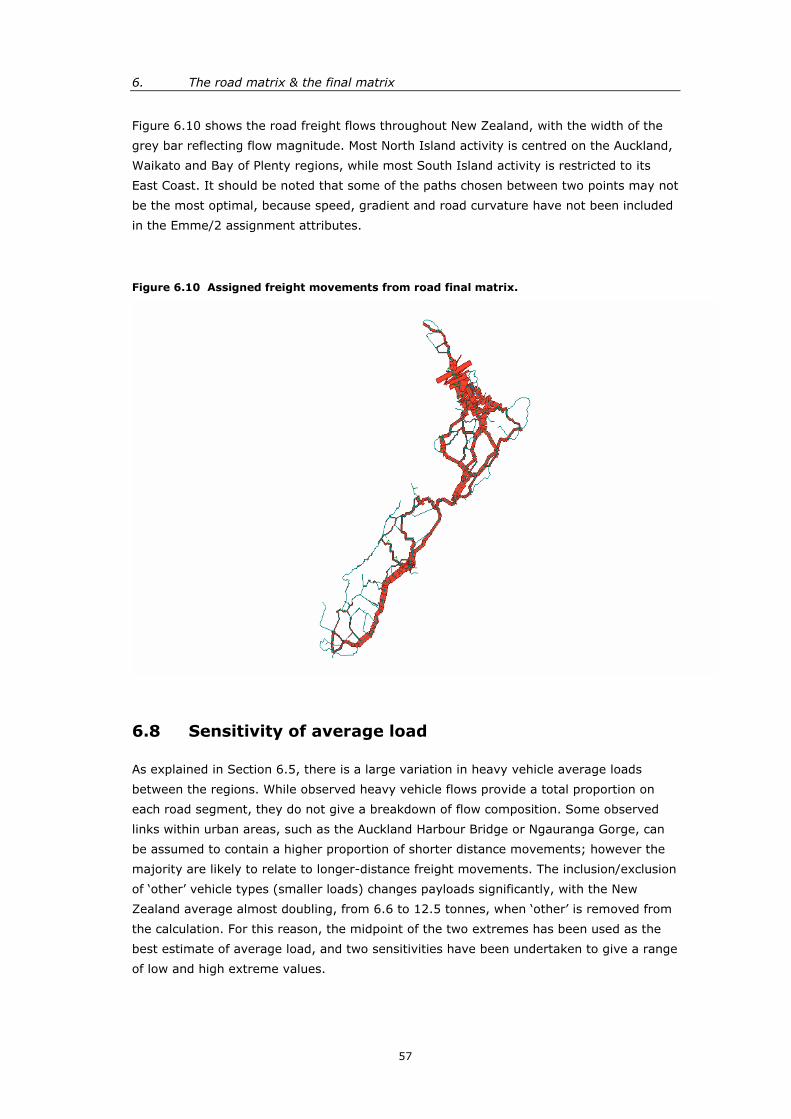
6. The road matrix & the final matrix
57
Figure 6.10 shows the road freight flows throughout New Zealand, with the width of the
grey bar reflecting flow magnitude. Most North Island activity is centred on the Auckland,
Waikato and Bay of Plenty regions, while most South Island activity is restricted to its
East Coast. It should be noted that some of the paths chosen between two points may not
be the most optimal, because speed, gradient and road curvature have not been included
in the Emme/2 assignment attributes.
Figure 6.10 Assigned freight movements from road final matrix.
6.8 Sensitivity of average load
As explained in Section 6.5, there is a large variation in heavy vehicle average loads
between the regions. While observed heavy vehicle flows provide a total proportion on
each road segment, they do not give a breakdown of flow composition. Some observed
links within urban areas, such as the Auckland Harbour Bridge or Ngauranga Gorge, can
be assumed to contain a higher proportion of shorter distance movements; however the
majority are likely to relate to longer-distance freight movements. The inclusion/exclusion
of ‘other’ vehicle types (smaller loads) changes payloads significantly, with the New
Zealand average almost doubling, from 6.6 to 12.5 tonnes, when ‘other’ is removed from
the calculation. For this reason, the midpoint of the two extremes has been used as the
best estimate of average load, and two sensitivities have been undertaken to give a range
of low and high extreme values.

DEVELOPMENT OF A NZ NATIONAL FREIGHT MATRIX
58
The midpoint payload is used in the conversion from link-based vehicle flows to freight
flows. Changing the assumption about average payload only affects the second part of the
matrix estimation process, from the seed matrix to the final matrix, and therefore, all
three scenarios have the same seed matrix.
Table 6.7 shows the impact of changing the assumption about average payload. As shown
in the previous section, the ‘midpoint load’ assumption results in 89.6million tonnes and
12.9 billion tonne-km. A more conservative view of average payloads (‘low load’) reduces
the total freight movements to 70.2 million tonnes (-22%) and tonne-km to 9.4 billion
(-27%). The average trip length is also lower at 134 km (-7%). The upper bound (or ‘high
load’) dramatically increases the final matrix, with freight movements at 180 million
tonnes (+21%) and tonne-km at 16.5 billion (+28%). The average trip length under this
scenario is also higher at 153 km (+6%). Changing the assumptions relating to average
payload gives a +/-20% bound for freight movements and +/-30% bound for freight km,
with the larger payloads encouraging longer trips.
Because of the large sensitivity of the matrix to these assumptions, further work needs to
be undertaken on average loads at each of the heavy-vehicle reporting sites. A
breakdown in the proportion of A, B, and R-type vehicles would be useful in that it could
be related to the HVLP and a better estimate at each site (rather than at a regional level)
could be undertaken.
Table 6.7 Impact of load assumptions on final road matrix.
Matrix Tonnage(million)
Tonne-km(million)
Average TripLength (km)
Seed (used for all) 51.1 6818 133.4
Midpoint Load
Difference 38.5 6,105 158.5
Total Midpoint Load 89.6 12,923 144.2
Low Load
Difference 19.1 2,591 135.6
Total Low Load 70.2 9,409 134.0
High Load
Difference 57.1 9,723 170.3
Total High Load 108.2 16,541 152.9
6.9 Combining road with rail
Once the road matrix had been generated through the modelling process, it was
combined with the previously described rail matrix (Section 5.6) to create a total land
transport matrix of freight movements, shown in Table 6.8. This total matrix largely
reflects the road matrix trends (as expected given the high mode share of road) and
shows that the Auckland region again dominates in both production (21% of total) and
attraction (22% of total) of freight movements. Waikato (contributing 20% of productions
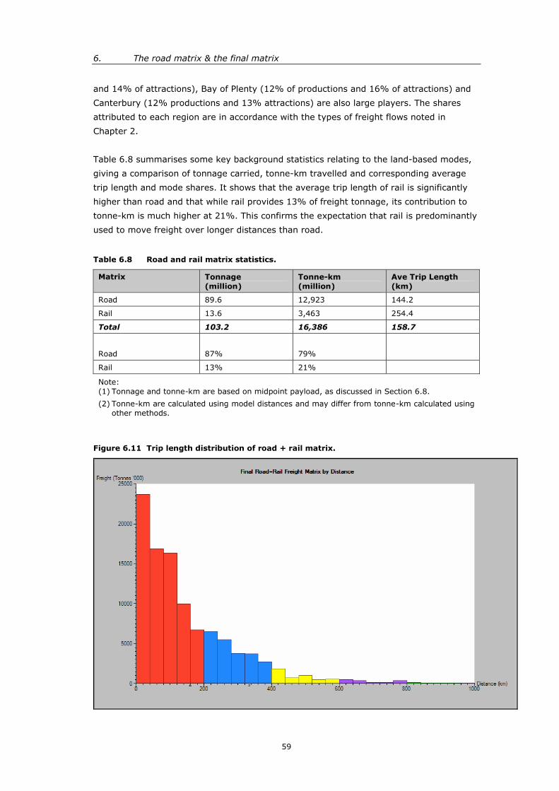
6. The road matrix & the final matrix
59
and 14% of attractions), Bay of Plenty (12% of productions and 16% of attractions) and
Canterbury (12% productions and 13% attractions) are also large players. The shares
attributed to each region are in accordance with the types of freight flows noted in
Chapter 2.
Table 6.8 summarises some key background statistics relating to the land-based modes,
giving a comparison of tonnage carried, tonne-km travelled and corresponding average
trip length and mode shares. It shows that the average trip length of rail is significantly
higher than road and that while rail provides 13% of freight tonnage, its contribution to
tonne-km is much higher at 21%. This confirms the expectation that rail is predominantly
used to move freight over longer distances than road.
Table 6.8 Road and rail matrix statistics.
Matrix Tonnage(million)
Tonne-km(million)
Ave Trip Length(km)
Road 89.6 12,923 144.2
Rail 13.6 3,463 254.4
Total 103.2 16,386 158.7
Road 87% 79%
Rail 13% 21%
Note:(1) Tonnage and tonne-km are based on midpoint payload, as discussed in Section 6.8.
(2) Tonne-km are calculated using model distances and may differ from tonne-km calculated usingother methods.
Figure 6.11 Trip length distribution of road + rail matrix.

DEVELOPMENT OF A NZ NATIONAL FREIGHT MATRIX
60
Figure 6.11 provides a trip length distribution of the combined road and rail matrix. This
distribution contains virtually the same proportion of freight movements of less than
200 km when compared with road. However it shows a greater proportion of movements
between 200 km and 400 km (at 22% rather than 20%) indicating that a larger
proportion of rail freight is of medium distance.
In summary, the final matrix shows that Auckland, Waikato, Bay of Plenty and Canterbury
are the dominant freight producing and receiving regions. Many freight movements are
intra-regional, and most are over the relatively short distances in which road dominates,
with a high proportion of less than 200 km distance. Rail has greatest mode share in the
medium and longer distance freight corridors.

6. The road matrix & the final matrix
61
Table 6.9 Estimated road and rail freight matrix (annual tonnes ‘000).
Nor
thla
nd
Auc
klan
d
Wai
kato
Bay
ofP
lent
y
Gis
born
e
Hawke’s Bay
Tar
anak
i
Man
awat
u-
Wan
ganu
i
Wel
lingt
on
Tas
man
Nel
son
Mar
lbor
ough
Wes
tCoa
st
Can
terb
ury
Ota
go
Sou
thla
nd
TO
TA
L
Northland 2,226 469 295 108 3 2 18 5 1 0 0 0 0 1 0 1 3,129
Auckland 567 15,377 2,961 1,590 55 91 100 167 179 0 6 15 1 340 29 10 21,488
Waikato 271 4,090 8,312 5,400 94 331 760 777 449 45 12 26 1 74 6 3 20,651
Bay of Plenty 44 2,211 1,692 7,589 219 52 174 290 108 2 1 3 0 30 4 2 12,421
Gisborne 6 57 98 384 520 133 12 98 85 9 3 6 0 7 1 0 1,419
Hawke’s Bay 5 86 193 236 226 1,452 124 470 230 15 5 10 0 53 7 3 3,116
Taranaki 19 318 517 236 29 98 2,005 465 319 5 3 4 1 31 5 1 4,057
Manawatu-Wanganui 9 217 479 589 245 370 1,156 787 1,109 19 5 12 1 70 5 2 5,074
Wellington 3 139 186 229 125 127 327 1,178 1,985 122 51 94 4 181 32 4 4,785
Tasman 0 1 13 18 11 7 18 24 138 766 746 197 28 81 42 0 2,091
Nelson 0 7 2 3 2 2 0 3 32 342 133 100 113 164 117 0 1,021
Marlborough 0 37 15 30 17 11 13 23 153 410 115 282 16 509 49 13 1,694
West Coast 0 2 2 3 0 0 5 6 8 31 24 26 380 2,439 26 3 2,955
Canterbury 2 142 63 69 6 12 83 174 77 124 319 746 462 8,517 1,183 442 12,421
Otago 0 28 4 6 1 3 9 13 13 11 16 40 7 624 1,748 759 3,282
Southland 0 15 6 4 0 6 8 8 5 3 2 15 23 529 858 2,159 3,640
TOTAL 3,153 23,196 14,838 16,495 1,552 2,698 4,810 4,488 4,889 1,904 1,441 1,575 1,039 13,649 4,112 3,404 103,243
From
To

DEVELOPMENT OF A NZ NATIONAL FREIGHT MATRIX
62
7. Examination of freight-trip-end model
7.1 Introduction
This chapter examines the possibility of developing a total freight-trip-end model (i.e.
including both road and rail), and whether it would be a suitable simplification to the
previously applied matrix estimation process.
A trip-end model for freight origins takes the matrix-estimated freight productions (total
freight originating by TLA in this case) and tries to relate these to explanatory variables
(also at a TLA level). A similar approach can be taken for freight destinations. Explanatory
variables are assumed to relate linearly to the productions/attractions, and accordingly
multiple linear regression is the statistical technique used.
Trip-end productions (by origin) and attractions (by destination) can be used in
conjunction with a distance matrix (using a gravity model as used in the matrix
estimation process) to give a new matrix estimate assuming the same average trip
length. The advantage of this process over the full matrix estimation approach is that it is
simpler to implement (once models are determined), does not require detailed data
collection from industry or freight operators, and gives the ability to crudely estimate
future year matrices. All that is potentially needed for future forecasts is a projection of
the explanatory variables and a view of any changes in average trip length. Note that the
resulting matrix is not as accurate as the fully estimated matrix, but it can be viewed as a
good approximation of it.
7.2 Data used
The variables used in this analysis were obtained from the Statistics New Zealand
website, which has datasets for the 2001 year that can be downloaded at a TLA level.
These include demographic information, such as population by age group and total
number of households, and employment statistics by industry and by full or part-time
classification (full-time equivalent (FTE) employment was estimated by taking full-time +
0.5 × part-time).
Table 7.1 shows employment segments and the associated FTE total for the whole
country. A final column has been added to the table to show the expected directed
influence of the employment sector on freight production and/or attraction. We would
expect some sectors to be generators of freight (such as agriculture, forestry and fishing;
mining; or manufacturing) and these are shown with a plus (+), while others to have a
negative impact on freight (such as service-based industries or education) and these are
shown with a minus (-). Some industries are not as easy to classify and so have been
given a question mark (?). These were the hypotheses by which conclusions were drawn
regarding the suitability of trip-end relationships that were derived.

7. Examination of freight-trip-end model
63
Table 7.1 Employment variables used for trip-end model examination.
EmploymentSegment
Description Total NZ FTEEmployed
ExpectedImpact on
Freight
AFF Agriculture, Forestry and Fishing 111,384 +
MIN Mining 2,622 +
MAN Manufacturing 191,609 +
EGW Electricity, Gas and Water 4,968 +
CON Construction 69,465 +
WST Wholesale Trade 83,057 +
RLT Retail Trade 158,508 +
ACR Accommodation, Cafes and Restaurants 58,554 ?
TAS Transport and Storage 48,887 ?
COM Communication Services 17.421 –
FIN Finance and Insurance 44,322 –
PRO Property and Business Services 156,906 –
GAD Government Admin. And Defence 50,793 –
EDU Education 101,352 –
HCS Health and Community Services 105,102 –
CRS Cultural and Recreational Services 31,014 –
PER Personal and other Services 48,539 ?
POP 2001 Total Population 3,736,101 ?
7.3 Origin and Destination trip-end model estimation
The trip-end models are linear multi-variate, and relate freight productions/attractions by
origin/destination TLA, with TLA specific employment by sector and/or population. One of
the difficulties when using employment by sector is that there is a high level of correlation
between most of the variables. Correlation is a measure of the degree to which behaviour
of one variable mirrors the behaviour of another: if correlation is high (close to +/- 1)
then either variable could be used as a substitute for the other. Including both variables
in the equation does not add anything to the model, and may affect the significance or
sign of the coefficient of the other.
The correlation matrix (refer Table E4 in Appendix E) shows that only AFF and MIN are
distinctly different from the other variables, with low correlation values. GAD is only
marginally correlated, while the rest are extremely similar and could be substitutes for
each other in the equation. As such, developing a robust set of equations is difficult, as
removal of a highly correlated variable from the analysis is likely to change other
variables it is correlated with, particularly in terms of sign and significance.
To derive an appropriate trip-end model, all variables were included in the initial model.
One by one, variables were excluded and the model re-estimated, a process known as
step-wise regression. Exclusion of variables was based on the extent to which a variable’s

DEVELOPMENT OF A NZ NATIONAL FREIGHT MATRIX
64
parameter value was statistically significantly different from zero, whether it was highly
correlated with another variable that had been included, or whether the expected sign of
the coefficient was correct (positive or negative). A constant was also included to allow for
any freight not explained by the variables.
After initial model estimations, significant outliers (where the modelled estimation was
very different from the observed values) were found. Further examination identified some
of these as TLAs with ports and it was found that employment categories were not
disaggregated enough to give an indication of port-based activity. It would be expected
that the loading/unloading of freight at ports would have a positive impact on freight
movements to/from port TLAs and, for this reason, two further variables were created to
represent port existence and relative size (see Appendix E).
7.3.1 Origin trip-end model
The following process was undertaken to arrive at an origin trip-end final formulation. The
number in brackets represents the adjusted R2, which indicates the level to which the
model corresponds to the observed data taking into account the number of variables
used. As variables are excluded, the adjusted R2 should increase if the model is improved:
• Start: All variables (0.616)
• Step 1: Exclude CON as not significant and wrong sign (0.622)
• Step 2: Exclude POP as not significant and wrong sign (0.629)
• Step 3: Exclude MAN as not significant and wrong sign (0.635)
• Step 4: Exclude RLT as not significant (0.640)
• Step 5: Exclude EGW as not significant (0.644)
• Step 6: Exclude COM as not significant (0.646)
• Step 7: Exclude GAD as not significant (0.650)
• Step 8: Exclude EDU as not significant and wrong sign (0.654)
• Step 9: Exclude CRS as not significant (0.655)
• Excluding any more variables had a negative impact on the adjusted R2
The final origin model parameters are listed in Table 7.2 which shows that all parameters
(other than the constant) are highly significant (different from zero, as indicated by a P-
value close to zero) to at least 10%.
A positive constant indicates that there are positive TLA freight production drivers not
explained by the variables included. A value of 5582 (5.6 million tonnes) for PORTORIG
gives an estimate of what the largest general import port (Auckland) would unload. This
compares with an observed figure of around 3.3 million tonnes for 2002. While the
estimated figure is higher, it should be noted that the observed number does not include
any coastal sea freight movements.
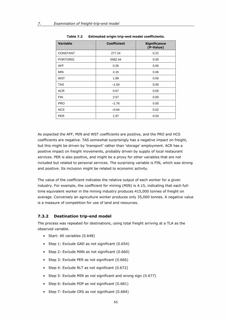
7. Examination of freight-trip-end model
65
Table 7.2 Estimated origin trip-end model coefficients.
Variable Coefficient Significance(P-Value)
CONSTANT 277.24 0.22
PORTORIG 5582.44 0.00
AFF 0.35 0.00
MIN 4.15 0.06
WST 1.99 0.00
TAS –1.04 0.00
ACR 0.67 0.05
FIN 2.57 0.00
PRO –1.76 0.00
HCS –0.64 0.02
PER 1.97 0.03
As expected the AFF, MIN and WST coefficients are positive, and the PRO and HCS
coefficients are negative. TAS somewhat surprisingly has a negative impact on freight,
but this might be driven by ‘transport’ rather than ‘storage’ employment. ACR has a
positive impact on freight movements, probably driven by supply of local restaurant
services. PER is also positive, and might be a proxy for other variables that are not
included but related to personal services. The surprising variable is FIN, which was strong
and positive. Its inclusion might be related to economic activity.
The value of the coefficient indicates the relative output of each worker for a given
industry. For example, the coefficient for mining (MIN) is 4.15, indicating that each full-
time equivalent worker in the mining industry produces 415,000 tonnes of freight on
average. Conversely an agriculture worker produces only 35,000 tonnes. A negative value
is a measure of competition for use of land and resources.
7.3.2 Destination trip-end model
The process was repeated for destinations, using total freight arriving at a TLA as the
observed variable.
• Start: All variables (0.648)
• Step 1: Exclude GAD as not significant (0.654)
• Step 2: Exclude MAN as not significant (0.660)
• Step 3: Exclude PER as not significant (0.666)
• Step 4: Exclude RLT as not significant (0.672)
• Step 5: Exclude MIN as not significant and wrong sign (0.677)
• Step 6: Exclude POP as not significant (0.681)
• Step 7: Exclude CRS as not significant (0.684)

DEVELOPMENT OF A NZ NATIONAL FREIGHT MATRIX
66
• Step 8: Exclude EGW as not significant and wrong sign (0.687)
• Step 9: Exclude EDU as not significant and wrong sign (0.690)
• Step 10: Exclude COM as not significant (0.693)
• Excluding any more variables had a negative impact on the adjusted R2
The final destination model parameters are listed in Table 7.3. All parameters other than
HCS are significant to at least 20%. Interestingly, the variables resulting from the model
estimation process bear a strong resemblance to the origin model in terms of sign and
magnitude. MIN is excluded and CON included, indicating that mining is a strong
generator of freight, and construction a strong attractor. PER is also excluded from the
destination model.
Table 7.3 Estimated destination trip-end model coefficients.
Variable Coefficient Significance(P-Value)
CONSTANT 315.90 0.17
PORTDEST 6201.14 0.00
AFF 0.28 0.01
CON 0.59 0.14
WST 1.79 0.00
TAS –1.00 0.00
ACR 0.51 0.18
FIN 2.67 0.00
PRO –1.49 0.00
HCS –0.24 0.27
A positive constant indicates that there are positive TLA freight attractor drivers not
explained by the variables included. A value of 6201 (6.2 million tonnes) for PORTDEST
gives an estimate of what the largest export port (Tauranga) would load. This compares
favourably with observed data of around 7.1 million tonnes for 2002.
All signs are consistent with the origin model, with parameter values being of a similar
magnitude, and most variables found to be significant in this model are also contained in
the origin model. This highlights the complex nature of freight movements, where an
industry can be a producer of freight in one leg of the process, but then an attractor
further down the production line (and vice versa).
7.3.3 Outliers
There are some significant outliers for both the origin and destination trip-end models.
These typically relate to areas where specific freight production or attraction facilities
have not been captured in the employment data.

7. Examination of freight-trip-end model
67
However with such general industry groupings it was not possible to represent these more
accurately. The exploration of industry employment at a more disaggregated level would
reduce the impact of this problem and might be an area for further work from this
project. Such data would provide a more detailed representation of the spread of relevant
industrial activity and allow the creation of a more accurate trip-end model.
7.4 Application
The purpose of this application was to produce an estimated matrix (Table 7.4) which
could be compared with the fully estimated matrix through matrix estimation procedures.
To achieve this, the trip-end origin and destination models and variable inputs were used
to create two vectors, providing an estimate of the total tonnage starting and finishing in
each TLA. These vectors were then read into the Emme/2 transport modelling package,
and a matrix-balancing procedure using an entropy function (see Chapter 6) was
undertaken to distribute trips by origin against trips by destination. This assumed the
same trip length as the final total freight matrix (158.7 km). The estimated matrix was
then compared with the total fully estimated matrix.
Initially the simplified regression process was found to overestimate shorter distance trips
and underestimate longer distance trips. To overcome this, differential functions (see
Appendix E for more information) were used for distances of less than and greater than
40 km. Figure 7.1 compares the final matrix (grey) with the estimated matrix using a
trip-end approach (white). The shaded area shows the overlap between the two.
Figure 7.1 Observed versus trip-end-estimated freight matrices by distance.

DEVELOPMENT OF A NZ NATIONAL FREIGHT MATRIX
68
Overall shorter-distance trips are underestimated by the trip-end approach, and medium-
distance trips are overestimated. Comparison of the two matrices at a TLA level gives
poor results (correlation of around 0.3), due to large differences being inherited from the
trip-end models. However, a comparison at a regional level (Figure 7.2) is more
favourable, with a correlation of 0.83 (where a correlation of ‘1’ would indicate a perfect
fit).
Figure 7.2 Scatterplot of fully-estimated versus trip-end-estimated regional freightmovements.
y = 1.0491xR2 = 0.8285
-
2,000
4,000
6,000
8,000
10,000
12,000
14,000
16,000
18,000
- 2,000 4,000 6,000 8,000 10,000 12,000 14,000
Estimated
Ob
serv
ed
A comparison of the resulting matrices from the two approaches (see difference matrices
in Tables 7.5 and 7.6) indicates an underestimation of intra-regional freight movements
by the trip-end approach (particularly for North Island regions), and an overestimation of
longer distance movements. Total freight movements are preserved through the
regression process which controls the constant to match the total. The largest origin
discrepancies relate to freight generated from Waikato and Bay of Plenty (which are
underestimated), and Hawke’s Bay and Manawatu-Wanganui (which are overestimated).
These regions also have the largest differences at the destination end. Trip-end total
differences indicate the fit of the trip-end regression models as discussed in Section 7.3.
The percentage differences between the fully-estimated and trip-end-estimated matrices
are large. All extreme values relate to minor flows and should be ignored, as a process
such as this is designed to represent larger flows, and it is assumed that the minor flows
would remain minor.

7. Examination of freight-trip-end model
69
There are large differences at a regional level, both in terms of productions and
attractions. These differences relate to the accuracy of the trip-end regression models in
matching actual levels. The use of a more disaggregated industry breakdown of
employment data might improve accuracy of the trip-end models in this respect. Any
errors in trip-ends have significant implications for individual region to region movements,
and these are indicated by the percentage differences in individual cells being generally
larger than the row or column differences.
While a fixed trip length gives an adequate fit, it does not provide a good representation
of short versus long distance freight. Further investigation would be required to determine
a more complex trip distribution function, which might be segmented into two or three
distance bands. A distribution function based on time rather than distance would allow the
development of a more representative road network, which might also improve model fit.
Finally, the introduction of ‘k-factors’ could be explored. These would be used to modify
times/costs at a regional level within the matrix, to either correct for inaccuracies in the
network (to allow for the loading/unloading of freight over Cook Strait or for steep
winding roads that might be deterrent for freight travel for example) or to take into
account freight-movement perceptions/functions that could not be represented solely in
cost or travel time terms (such as contracts).
In summary, the trip-end approach does have some merit, giving a matrix of the same
broad shape as the fully-estimated approach whilst preserving total movements.
However, individual region to region movements have large errors, which are a function
of the accuracy of the regression equations and the trip length distribution used.

DEVELOPMENT OF A NZ NATIONAL FREIGHT MATRIX
70
Table 7.4 Trip-end-estimated total freight matrix (annual tonnes ‘000).
Nor
thla
nd
Auc
klan
d
Wai
kato
Bay
ofP
lent
y
Gis
born
e
Hawke’s Bay
Tar
anak
i
Man
awat
u-
Wan
ganu
i
Wel
lingt
on
Tas
man
Nel
son
Mar
lbor
ough
Wes
tCoa
st
Can
terb
ury
Ota
go
Sou
thla
nd
TO
TA
L
Northland 1,620 2,391 345 228 10 27 47 25 4 0 0 0 0 0 - - 4,698
Auckland 1,786 12,668 3,778 2,916 126 341 597 320 56 3 2 6 1 3 0 0 22,603
Waikato 354 4,985 2,918 3,298 179 669 892 603 118 5 5 13 2 6 0 0 14,046
Bay of Plenty 105 1,807 1,692 2,843 351 447 290 285 62 3 3 6 1 3 0 0 7,899
Gisborne 6 96 105 349 400 342 23 74 31 1 1 3 0 1 0 - 1,431
Hawke’s Bay 25 425 609 756 556 2,174 257 988 436 16 15 36 4 16 0 0 6,313
Taranaki 28 488 528 351 27 197 1,878 677 203 9 9 22 3 10 0 0 4,429
Manawatu-Wanganui 28 477 640 583 146 1,166 1,072 2,191 1,065 48 45 112 13 49 1 0 7,636
Wellington 5 88 132 134 63 533 320 1,108 1,581 120 113 279 33 122 1 0 4,634
Tasman 0 7 11 11 4 34 27 90 206 597 570 244 140 166 3 1 2,111
Nelson 0 2 2 2 1 7 6 19 42 125 60 50 21 25 0 0 364
Marlborough 1 14 20 20 7 63 49 166 377 193 181 304 62 375 4 1 1,837
West Coast 0 6 9 8 3 27 21 70 160 395 273 214 814 1,099 35 21 3,156
Canterbury 1 10 14 14 5 44 35 117 266 211 146 536 560 10,705 742 284 13,689
Otago 0 0 0 0 0 1 1 2 5 6 4 10 33 820 1,262 1,093 3,236
Southland 0 0 0 0 0 0 0 1 3 5 3 6 30 527 1,577 3,013 5,166
TOTAL 3,959 23,464 10,803 11,514 1,881 6,071 5,513 6,736 4,615 1,738 1,430 1,841 1,718 13,925 3,625 4,414 103,247
From
To
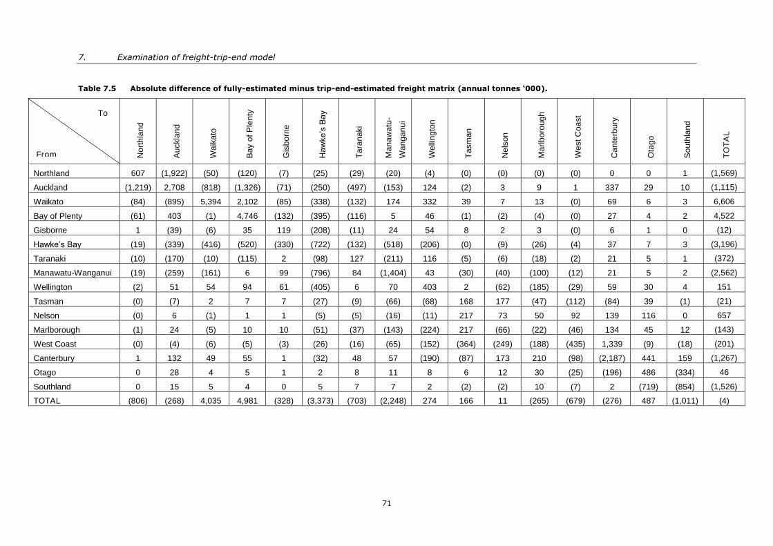
7. Examination of freight-trip-end model
71
Table 7.5 Absolute difference of fully-estimated minus trip-end-estimated freight matrix (annual tonnes ‘000).
Nor
thla
nd
Auc
klan
d
Wai
kato
Bay
ofP
lent
y
Gis
born
e
Hawke’s Bay
Tar
anak
i
Man
awat
u-
Wan
ganu
i
Wel
lingt
on
Tas
man
Nel
son
Mar
lbor
ough
Wes
tCoa
st
Can
terb
ury
Ota
go
Sou
thla
nd
TO
TA
L
Northland 607 (1,922) (50) (120) (7) (25) (29) (20) (4) (0) (0) (0) (0) 0 0 1 (1,569)
Auckland (1,219) 2,708 (818) (1,326) (71) (250) (497) (153) 124 (2) 3 9 1 337 29 10 (1,115)
Waikato (84) (895) 5,394 2,102 (85) (338) (132) 174 332 39 7 13 (0) 69 6 3 6,606
Bay of Plenty (61) 403 (1) 4,746 (132) (395) (116) 5 46 (1) (2) (4) (0) 27 4 2 4,522
Gisborne 1 (39) (6) 35 119 (208) (11) 24 54 8 2 3 (0) 6 1 0 (12)
Hawke’s Bay (19) (339) (416) (520) (330) (722) (132) (518) (206) (0) (9) (26) (4) 37 7 3 (3,196)
Taranaki (10) (170) (10) (115) 2 (98) 127 (211) 116 (5) (6) (18) (2) 21 5 1 (372)
Manawatu-Wanganui (19) (259) (161) 6 99 (796) 84 (1,404) 43 (30) (40) (100) (12) 21 5 2 (2,562)
Wellington (2) 51 54 94 61 (405) 6 70 403 2 (62) (185) (29) 59 30 4 151
Tasman (0) (7) 2 7 7 (27) (9) (66) (68) 168 177 (47) (112) (84) 39 (1) (21)
Nelson (0) 6 (1) 1 1 (5) (5) (16) (11) 217 73 50 92 139 116 0 657
Marlborough (1) 24 (5) 10 10 (51) (37) (143) (224) 217 (66) (22) (46) 134 45 12 (143)
West Coast (0) (4) (6) (5) (3) (26) (16) (65) (152) (364) (249) (188) (435) 1,339 (9) (18) (201)
Canterbury 1 132 49 55 1 (32) 48 57 (190) (87) 173 210 (98) (2,187) 441 159 (1,267)
Otago 0 28 4 5 1 2 8 11 8 6 12 30 (25) (196) 486 (334) 46
Southland 0 15 5 4 0 5 7 7 2 (2) (2) 10 (7) 2 (719) (854) (1,526)
TOTAL (806) (268) 4,035 4,981 (328) (3,373) (703) (2,248) 274 166 11 (265) (679) (276) 487 (1,011) (4)
From
To

DEVELOPMENT OF A NZ NATIONAL FREIGHT MATRIX
72
Table 7.6 Percentage difference (%) of fully-estimated minus trip-end-estimated freight matrix.
Nor
thla
nd
Auc
klan
d
Wai
kato
Bay
ofP
lent
y
Gis
born
e
Hawke’s Bay
Tar
anak
i
Man
awat
u-
Wan
ganu
i
Wel
lingt
on
Tas
man
Nel
son
Mar
lbor
ough
Wes
tCoa
st
Can
terb
ury
Ota
go
Sou
thla
nd
TO
TA
L
Northland 27 -410 -17 -111 -246 -1201 -163 -389 -729 -567 -428 -840 -1400 70 100 100 –50
Auckland -215 18 -28 -83 -128 -276 -497 -92 69 -1268 57 59 48 99 100 100 –5
Waikato -31 -22 65 39 -91 -102 -17 22 74 88 58 51 -1 93 99 99 32
Bay of Plenty -139 18 0 63 -61 -757 -66 2 43 -23 -319 -128 -78 90 99 99 36
Gisborne 11 -68 -7 9 23 -156 -93 25 64 88 61 55 -20 84 99 100 –1
Hawke’s Bay -368 -393 -216 -220 -146 -50 -106 -110 -89 -3 -181 -274 -956 70 97 98 –103
Taranaki -52 -53 -2 -49 5 -100 6 -45 36 -107 -185 -393 -228 69 98 97 –9
Manawatu-Wanganui -209 -119 -34 1 40 -215 7 -178 4 -160 -833 -853 -1479 30 90 92 –50
Wellington -70 37 29 41 49 -318 2 6 20 1 -122 -197 -753 32 96 88 3
Tasman -330 -1267 16 40 64 -375 -53 -270 -49 22 24 -24 -399 -104 94 -316 –1
Nelson -73 79 -35 25 52 -236 -1384 -632 -33 63 55 50 81 85 100 47 64
Marlborough -282 64 -35 33 56 -450 -292 -626 -146 53 -57 -8 -286 26 92 89 –8
West Coast -286 -281 -295 -176 -1224 -8106 -298 -1103 -1957 -1163 -1034 -723 -115 55 -33 -583 –7
Canterbury 71 93 78 80 13 -268 58 33 -248 -70 54 28 -21 -26 37 36 –10
Otago 85 99 94 95 91 72 93 84 62 49 75 76 -345 -31 28 -44 1
Southland 88 99 97 97 43 91 95 84 37 -86 -85 62 -30 0 -84 -40 –42
TOTAL % –26 –1 27 30 –21 –125 –15 –50 6 9 1 –17 –65 –2 12 –30 0
From
To

8. Conclusions
73
8. Conclusions
8.1 Main findings
This study has investigated the movement of freight within New Zealand. Through the
survey of freight consignors and carriers, the use of other data sources and the Emme/2-
based estimation process, it has estimated the main long-distance high tonnage freight
movements within the country during the year 2002. It has assembled matrices of
movements for the main land transport modes of road and rail, listing the approximate
tonnages moving between and within origin and destination regions during that year. An
indication of the significant commodities and industries utilising the freight networks has
also been provided, although such information has not been incorporated into the
matrices. This is the first time in New Zealand that such matrices have been attempted or
that inter-regional freight movement has been investigated in this detail.
The main findings are:
• Of the three main modes (road, rail, shipping), road transport conveys the majority
of freight within New Zealand, having an approximate 83% share of tonnage and a
67% share of tonne-km. Rail has an approximate 13% of tonnage and 18% of
tonne-km, and coastal shipping has a corresponding 4% of tonnage and 15% of
tonne-km. Road has the shortest average haul of the three main modes, while
coastal shipping (excluding the inter-island ferries) has the longest.
• Three regions –Auckland, Waikato and Bay of Plenty –are responsible for the
production and attraction of over half of all road and rail freight, reflecting a
concentration of population and industry. Canterbury, the largest region by area, is
the only other region with a share of more than 10% of freight productions and
attractions.
• Over two thirds of all road movements are of less than 200 km, with the Auckland
region dominating with around a quarter of both the production and attraction of all
freight. The greatest road tonnage corridors are, in descending order, Auckland to
Auckland, Canterbury to Canterbury, Waikato to Waikato, Bay of Plenty to Bay of
Plenty, Waikato to Auckland, and Waikato to Bay of Plenty. These corridors account
for nearly half of all road freight tonnage and show a preponderance by road to
short-haul movements.
• Higher rail tonnages correspond to the locations of major industrial plants, mines
and ports. The greatest tonnage corridors for rail are, in descending order, Bay of
Plenty to Bay of Plenty, West Coast to Canterbury, and Waikato to Bay of Plenty.
These three corridors account for nearly half of all rail tonnage.
• A significant proportion (over half) of all freight cannot be easily classified into the
specific commodity groups as defined. This includes general freight movements,
and those relating to wholesale/retail, construction and other business sectors.
DEVELOPMENT OF A NZ NATIONAL FREIGHT MATRIX
74
• The primary industries of agriculture and forestry are the largest originators of
freight that can be categorised into a specific commodity group. The transport of
logs, milk and livestock account for a significant share of total freight movements.
• A trip-end model for freight origins and destinations shows some correlation to the
modelled matrix, but further improvements in both the data and process would be
required to achieve a reasonable level of accuracy.
It should be noted that the results of this study have been limited by the availability of
data and the associated assumptions that have been made. The issue of commercial
confidentiality reduced both participation in the survey phase and the usefulness of the
data supplied. This coupled with the lack of statistics measuring freight and commodity
data by weight have restricted the detail that could be included. Additionally, the
constantly evolving nature freight transport market has limited the results presented here
to a snapshot only, of the economy as it was in 2002. Nonetheless, the work is a
considerable advance on anything available previously.
8.2 Improvements to developing a freight matrix
A number of recommended improvements could be made to the processes of developing
the freight matrix presented in this report, which would allow a more detailed matrix to
be developed and enhance the detail and results available.
For the full matrix such improvements would include:
• The compilation, by organisations such as Statistics New Zealand, of detailed
statistics relating to weight of goods transported. Where data is currently collected,
it is often recorded using measures other than weight, limiting its usefulness for
tasks such as this.
• The collection of more complete observed data, by Transit New Zealand and other
organisations, such as the split of heavy vehicle types at telemetry sites.
• The use of better estimates of average loads, which would improve the accuracy of
the estimation process by limiting assumptions. The improvements to the collection
of data listed above might allow better estimates to be prepared.
• Review the annualisation factor used in conjunction with AADT to relate this more
to the movements of commercial vehicles. Average daily flows are currently
designed primarily to match general traffic patterns that are dominated by car
journeys, and they may therefore underestimate the weekday-oriented patterns
associated with commercial vehicles.
• Improvement of the Emme/2 network and functions to take account of speed,
gradient, and road curvature, etc. This would allow a more accurate model of the
national transportation networks to be developed.
For the trip end approach such improvements would include:
• The collection of more disaggregated industry employment data for the trip end
model.

8. Conclusions
75
• The investigation of the feasibility of introducing k-factors to balancing process.
This would allow times or costs to be modified, to correct for inaccuracies in the
network or take account of perceptions and functions.
8.3 Further work
Three principal directions that future work might take are:
• The ongoing monitoring of the freight sector, which might involve the update of the
model every 2-3 years, to measure historical trends and increase knowledge of the
factors affecting the movement of freight in the New Zealand context.
• Use of the model to forecast future freight movements. This would be a valuable
tool for the planning of future requirements for roads, railways, ports and other
freight facilities.
• The application of this process to create detailed freight matrices at the regional or
even TLA level. These would have a higher level of detail and could be combined as
required to look at freight movements within a specific geographic area (for
example, the southern South Island).

DEVELOPMENT OF A NZ NATIONAL FREIGHT MATRIX
76
77
Appendix A References
The references contained in the main report and the appendices are listed here.
Austroads. 2003. Forecasting inter-regional freight transport from regional development.
Booz Allen Hamilton. 2003. Clifford Bay ferry terminal demand assessment.
Cavana, R.Y., Harrison, I.G., Heffernan, F.E.B., Kissling, C.C. 1997. Freight transport
industry in New Zealand. GSBGM Working Paper Series 2/97, Victoria University of
Wellington.
HortResearch. 2004. New Zealand horticulture facts & figures 2002. An annual publication
compiled by Martech Consulting Group for HortResearch (The Horticulture and
Research Institute of New Zealand).
King, M.A. 1971. The structure and ownership of the New Zealand licensed road goods
transport industry. Unpublished doctoral thesis, Victoria University of Wellington.
Livestock Improvement Corporation. 2003. Dairy statistics 2002-2003. Retrieved from
www.lic.co.nz
Meat & Wool Innovation –Economic Service. 2003. Annual review of the sheep & beef
industry 2002-03.
Ministry of Agriculture and Forestry (MAF). 2004a. General statistics from the MAF
website at www.maf.govt.nz
Ministry of Agriculture and Forestry (MAF). 2004b. National exotic forest description as at
1 April 2003. Published by MAF in April 2004. Available from the MAF website at
http://www.maf.govt.nz/statistics
Ministry of Economic Development. 2004. General statistics from MED website at
www.med.govt.nz
Ministry of Transport. 2005a. Coastal shipping cargo: 2004/05. Available from Ministry of
Transport website at www.mot.govt.nz
Ministry of Transport. 2005b. Surface transport costs and charges. Study prepared by
Booz Allen Hamilton for MOT, Wellington, New Zealand.
NZ Institute of Economic Research (NZ IER). 2002. Transport and economic growth:
coupled, decoupled or coupling? A report to the New Zealand Ministry of Transport.
Road Transport Forum NZ (RTF NZ). 2005. Road Transport Forum website at
www.rtfnz.co.nz
Road Transport Forum NZ. 2004. Road Transport Facts. Statistical publication produced
by the Road Transport Forum.

DEVELOPMENT OF A NZ NATIONAL FREIGHT MATRIX
78
Statistics New Zealand. 2003a. Overseas trade imports and exports by port. Sourced from
Statistics New Zealand.
Statistics New Zealand. 2003b. Agriculture statistics 2002. Available at the Statistics New
Zealand website.
Statistics New Zealand. 2004. General statistics from the Statistics New Zealand website
at http://www.stats.govt.nz/default.htm
Transit New Zealand. 2001. Heavy vehicle limits project (HVLP): Report 4 –industry
economics.
Transport & Population Data Centre. 2002. Commercial Transport Study. Details available
at the Transport & Population Data Centre website at www.planning.nsw.gov.au/tpdc
Tranz Rail. 2003. Tranz Rail Holdings Annual Report 2003.
TERNZ (Transport Engineering Research NZ). 2004. Profile of the heavy vehicle fleet:
Update 2004. Prepared for the Road Safety Trust.
TERNZ. 2003. Heavy vehicle movements in New Zealand. Prepared for Land Transport
Safety.