Requirements for Hybrid Cosimulation - Simulation...

Requirements for Hybrid Cosimulation

David BromanLev GreenbergEdward A. LeeMichael MassinStavros TripakisMichael Wetter

Electrical Engineering and Computer SciencesUniversity of California at Berkeley

Technical Report No. UCB/EECS-2014-157http://www.eecs.berkeley.edu/Pubs/TechRpts/2014/EECS-2014-157.html

August 16, 2014

Copyright © 2014, by the author(s).All rights reserved.

Permission to make digital or hard copies of all or part of this work forpersonal or classroom use is granted without fee provided that copies arenot made or distributed for profit or commercial advantage and thatcopies bear this notice and the full citation on the first page. To copyotherwise, to republish, to post on servers or to redistribute to lists,requires prior specific permission.

Acknowledgement

This work is supported in part by the iCyPhy Research Center (IndustrialCyber-Physical Systems, supported by IBM and United Technologies), andthe Center for Hybrid and Embedded Software Systems (CHESS) at UCBerkeley (supported by NSF award #0931843 (ActionWebs), NRL award#N0013-12-1-G015, the Assistant Secretary for Energy Efficiency andRenewable Energy, Office of Building Technologies of the U.S. DoE, underContract No. DE-AC02-05CH11231, and the following companies: Denso,National Instruments, and Toyota). This work was also supported by theAcademy of Finland and by the NSF via projects COSMOI: CompositionalSystem Modeling with Interfaces and ExCAPE: Expeditions in ComputerAugmented Program Engineering. This work was also supported by the Swedish Research Council #623-2013-8591.

Requirements for Hybrid Cosimulation ∗

David Broman1,2, Lev Greenberg3, Edward A. Lee1,Michael Masin3, Stavros Tripakis1,4, Michael Wetter5

1{broman,eal,stavros}@eecs.berkeley.edu, 3{levg,michaelm}@il.ibm.com, [email protected] of California, Berkeley, 2KTH Royal Institute of Technology,

3IBM Research – Haifa, Israel, 4Aalto University, 5Lawrence Berkeley National Laboratory

August 16, 2014

Abstract

This paper defines a suite of requirements for future hybrid cosimulation standards, and specificallyprovides guidance for development of a hybrid cosimulation version of the Functional Mockup Interface(FMI) standard. A cosimulation standard defines interfaces that enable diverse simulation tools tointeroperate. Specifically, one tool defines a component that forms part of a simulation model in anothertool. We focus on components with inputs and outputs that are functions of time, and specifically oninputs and outputs that are mixtures of discrete events and continuous time signals. This hybrid mixtureis not well supported by existing cosimulation standards, and specifically not by FMI 2.0, for reasonsthat are explained in this paper. The paper defines a suite of test components, giving a mathematicalmodel of an ideal behavior, plus a discussion of practical implementation considerations. The discussionincludes acceptance criteria by which we can determine whether a standard supports definition of eachcomponent. In addition, the paper defines a set of test compositions of components. These compositionsdefine requirements for coordination between components, including consistent handling of timed events.

1 Introduction

FMI (Functional Mock-up Interface) is an evolving standard for composing model components designed usingdistinct modeling and simulation tools [16]. The standard consists of a C API for simulation components andan XML schema for describing components. An FMU (Functional Mock-up Unit) is a component, typicallyexported from a modeling and simulation tool, that can be instantiated and used as part of a simulationin another modeling tool. To date, the emphasis of the standard has been on components that model thedynamics of physical systems, such as mechanical and electrical components. This emphasis reflects theorigins of FMI as a way to achieve interoperability of simulators for models of automotive suppliers andOEMs [4].

FMI provides two distinct mechanisms for interaction between an FMU and a host simulator. Thefirst mechanism is model exchange, where the host simulator is responsible for all numerical integrationmethods. The FMU provides procedures representing model equations, for example to compute the derivativeof state variables of the component given current values for those state variables. The host simulator

∗Acknowledgments: This work was supported in part by the iCyPhy Research Center (Industrial Cyber-Physical Systems,supported by IBM and United Technologies), and the Center for Hybrid and Embedded Software Systems (CHESS) at UCBerkeley (supported by the National Science Foundation, NSF award #0931843 (ActionWebs), the Naval Research Laboratory(NRL #N0013-12-1-G015), the Assistant Secretary for Energy Efficiency and Renewable Energy, Office of Building Technologiesof the U.S. Department of Energy, under Contract No. DE-AC02-05CH11231, and the following companies: Denso, NationalInstruments, and Toyota). This work was also supported by the Academy of Finland and by the NSF via projects COSMOI:Compositional System Modeling with Interfaces and ExCAPE: Expeditions in Computer Augmented Program Engineering.This work was also supported by the Swedish Research Council #623-2013-8591.

1

is responsible for advancing time and updating the values of state variables, for example by performingnumerical integration.

The second mechanism is cosimulation, where the FMU implements its own mechanisms for advancingthe values of state variables, for example by internally implementing its own numerical integration method.The host simulator provides input values to the FMU, requests that the FMU advance its state variablesand output values in time, and then queries for the updated output values. Cosimulation provides a loosercoupling of tools than model exchange, and in principle can have a smaller, simpler interface with fewerassumptions and constraints. In the FMI 2.0 standard [16], both of these mechanisms, but most particularlycosimulation, are optimized for simulating continuous dynamics. The emphasis in model exchange is onproviding enough information about the FMU component so that the host simulator can effectively usesophisticated integration algorithms. The emphasis in cosimulation is on loose coupling between continuousintegration algorithms, where time can advance somewhat independently within the FMU and the hostsimulator. For example, the current version of the standard provides no mechanism for a cosimulationFMU to output an instantaneous reaction to a changed input value (such reactions are central to reactivesystems [7]). The assumption is that inputs and outputs change reasonably smoothly, so delayed reactionshave small effects on the overall simulation behavior.

In view of these assumptions, the community-driven standardization process is considering a third mech-anism called hybrid cosimulation that strives for the loose coupling of cosimulation, but with supportfor discrete and discontinuous signals and instantaneous events. The intent of this mechanism is to supporthybrid systems [13, 1, 6, 19, 17], where continuous dynamics are combined with discrete mode changes anddiscrete events. Any mechanism that supports hybrid systems can also support purely discrete systems andpurely continuous systems, since those are both special cases.

In this paper, we provide a series of examples of simulation components (test components) that must besupported by any comprehensive mechanism that supports hybrid systems. These examples are chosen tocomprehensively cover the space of functionality needed to effectively model mixed continuous and discretesystems, and to be as simple as possible. In addition, we provide a small set of simulation models (testmodels) that compose test components. For the test components and models, we mathematically definean ideal behavior and discuss practical acceptance criteria by which we can determine whether a practicalimplementation conforms with the ideal behavior.

Note that although FMI 2.0 does not currently support hybrid cosimulation, small extensions to thestandard are sufficient to enable such support. Some such extensions are described and analyzed in [5,21], where it is shown for example how to support reactive systems. We believe, therefore, that a hybridcosimulation FMI standard that conforms with the requirements in this paper and yet is similar in spiritand style to the current standard is practical.

Together with the FMI 2.0 standards document, the FMI Development Group has developed an FMITest Package. This package provides a number of models given in the Modelica language [15, 20], togetherwith a specification of submodels that should be exported by a tool as FMUs, and re-imported by a toolas FMU. A tool passes the test if the behaviors all match the Modelica behavior. Compatibility betweentools can be checked by having one tool import FMUs exported by another. If all tests match the Modelicabehavior, the tools are compatible.

Although we could find no explicit statement to this effect, the tests specified in this package appearto be tests of the Model Exchange mechanism in FMI 2.0, since many of the tests are not implementableusing Co-Simulation. Nevertheless, many of these tests are just as relevant to a future Hybrid Cosimulationstandard as they are to the existing Model Exchange standard. Those tests include simple connections thattest for proper FMU sorting, connections with cycles (that can be resolved without algebraic loop solving),linear and non-linear systems, systems with mixed data types, systems with event propagation, and modelsthat test initialization of connected FMUs. Most (and possibly all) of these test cases could also form usefultest cases for a Hybrid Cosimulation standard. Hence, we mostly avoid in our test cases in this papersituations that are already covered by those tests.

In this paper, we also take a different approach towards specifying test cases. Instead of providing aModelica program as a reference, we give a mathematical ideal. The ideal correct behavior of a model is

2

unambiguous and language and tool independent.In some cases, the mathematical ideal is not exactly realizable by any computational system. Real

numbers, for example, are always approximated in a computational system, typically by floating pointnumbers. Such approximations are necessarily part of the test criteria, with specified tolerances.

Also, in some cases, the tests given here may not be directly realizable in Modelica, which, for example,lacks the notion of an absent value on a signal. These tests reflect discrete-event behaviors that are foundmore commonly in other types of simulators, such as network simulators (e.g. ns-3, http://www.nsnam.org/,and OPNET, from Riverbed)), hardware description languages (such as VHLD and SystemC), DEVS-basedsystem simulators [22], and synchronous-reactive languages [3]. Although these tests can be emulated inModelica through suitable encoding of signals, and Modelica tools should be able to import FMUs using thisnotion through such suitable encodings, it would be awkward and indirect to specify the tests in this way.

2 Principles

2.1 Definitions

We adopt the following definitions:

• A host simulator is a tool that imports a modeling component (an FMU) that is either written by handor exported from another tool (or possibly even the same tool).

• The master algorithm is the execution procedure and policy by which the host simulator invokes theinterface procedures of a component (an FMU).

• A communication point is the simulation time at which the master algorithm invokes an interfaceprocedure of an FMU.

• A deterministic FMU is one where the output values and states are uniquely defined given initialconditions, input values, and communication points.

• A deterministic composition of deterministic FMUs is one where for a valid sequence of commu-nication points, given initial conditions and inputs from outside the composition, the values of outputsof the deterministic FMUs are uniquely defined. Note that practical implementations may approximatethose values using imprecise numerical methods, but the composition is still deterministic if the idealcorrect values are uniquely defined.

The definition of determinism is a bit subtle. See [10] for a rigorous definition.

2.2 Assumptions

The FMI specification for hybrid cosimulation defines a contract between FMUs and master algorithms.This paper assumes the following principles to be followed in defining the specification:

• We prefer a weaker contract over a stronger contract. That is, we prefer fewer constraints on the design ofFMUs and master algorithms. Constraints that can be eliminated without violating the requirements ofthis document should be eliminated. This will maximize interoperability of FMUs and master algorithms.

• We assume superdense time and piecewise continuous signals (see below and [11]). Specifically, two distinctcommunication points can share the same notion of real simulation time and yet be ordered in time. Thisis necessary for rigorous modeling of discontinuities and discrete signals and is already included in FMI2.0 for model exchange.

• Where possible, the specification should use mechanisms already present in FMI 1.0 and 2.0, rather thanreplacing them with new mechanisms.

• The specification should enable, but not require, efficient execution.

2.3 Requirements

The FMI specification extension for hybrid cosimulation shall provide the following:

3

• It shall be able to handle all test cases that are described in this document, with approximations wherenecessary, as indicated in the discussion of the test cases below.

• It shall provide an unambiguous way of cosimulating FMUs.

• It shall enable (but not necessarily mandate) master algorithms that assure deterministic composition ofdeterministic FMUs.

• It shall be backwards compatible, meaning that current version 2.0 FMUs for cosimulation shall be possibleto simulate, at least with continuous inputs, together with new FMUs designed specifically for hybridcosimulation.

2.4 Notation

We use a particular mathematical notation to define the test cases in this paper. This notation is not intendedto be used explicitly in the FMI specification for hybrid cosimulation. It is a mathematical idealization ofwhat would be realized in an FMU and the host simulator.

The set T = R+ × N represents time, where R+ is the set of non-negative real numbers, and N ={0, 1, 2, · · · } is the set of natural numbers. A superdense time τ ∈ T is two-tuple, τ = (t, n), wherethe real number t represents a time in the usual Newtonian sense, and n is the microstep, which indexessequences of values at Newtonian time t. Every communication point is a member of the set T .

T is a totally ordered set, where for any τ1, τ2 ∈ T where τ1 = (t1, n1) and τ2 = (t2, n2), then τ1 > τ2 ifeither t1 > t2, or t1 = t2 and n1 > n2. Otherwise, τ1 ≤ τ2.

A signal x is a function of the formx : T → R ∪ {ε}, (1)

where ε represents the absence of a value. In the ideal, the signal is total, defined at all T , but in a simulation,signal values will be computed only at a finite subset of values of T . Note that the FMI specification willneed to deal with data types other than reals as well, but we assume here that those data types simplymatch what is provided by FMI 2.0. There is no need for a hybrid cosimulation standard to deviate fromthe existing standard in this regard. Also note that nothing in this paper requires that FMI include anyexplicit representation of ε. It is a semantical concept.

A continuous-time (CT) signal is one that has a non-absent value for all τ ∈ T . A discrete-event(DE) signal is one that has a non-absent value at only some τ ∈ T . Specifically, following [11], a DE signalx has a non-absent value x(τ) only for τ ∈ D ⊂ T , where D is a discrete set.1

A signal is discontinuous at any time t ∈ R if there exist n,m ∈ N such that x(t, n) 6= x(t,m).The initial-value signal xi for a signal x is a function of the form xi : R+ → R ∪ {ε} given by

xi(t) = x(t, 0)

for all t ∈ R+.At any t ∈ R+, the final microstep mt of a signal x is a number mt ∈ N such that for all m > mt,

x(t,m) = x(t,mt). The final value at time t is x(t,mt). If for any t ∈ R+, x has no final microstep, then xis said to be a chattering Zeno signal. It has a Zeno condition at time t, where it has an infinite sequenceof changing values. Put another way, for a chattering Zeno signal, there exists a time where the signal doesnot settle to a final value.

The final-value signal xf for a non-chattering Zeno signal x is a function of the form xf : R+ → R∪{ε}given by

xf (t) = x(t,mt)

for all t ∈ R+, where mt is the final microstep at time t.A continuous signal is a CT signal where for all t ∈ R+, mt = 0 and xi is continuous at t (in the usual

sense for functions of reals).A piecewise-continuous CT signal is one where

1A discrete set is an ordered set that is order isomorphic with a subset of the natural numbers [11].

4

1. mt = 0 for all t ∈ R+, except t ∈ D, where D ⊂ R+ is a discrete set.

2. xi is left-continuous for all t (in the usual sense for functions of reals).

3. xf is right-continuous for all t.

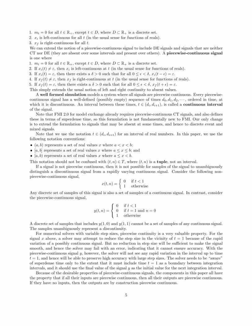
We can extend the notion of a piecewise-continuous signal to include DE signals and signals that are neitherCT nor DE (they are absent over some intervals and present over others). A piecewise-continuous signalis one where

1. mt = 0 for all t ∈ R+, except t ∈ D, where D ⊂ R+ is a discrete set.

2. If xi(t) 6= ε, then xi is left-continuous at t (in the usual sense for functions of reals).

3. If xi(t) = ε, then there exists a δ > 0 such that for all 0 ≤ ε < δ, xi(t− ε) = ε.

4. If xf (t) 6= ε, then xf is right-continuous at t (in the usual sense for functions of reals).

5. If xf (t) = ε, then there exists a δ > 0 such that for all 0 ≤ ε < δ, xf (t+ ε) = ε.

This simply extends the usual notion of left and right continuity to absent values.A well formed simulation models a system where all signals are piecewise continuous. Every piecewise-

continuous signal has a well-defined (possibly empty) sequence of times d0, d1, d2, · · · , ordered in time, atwhich it is discontinuous. An interval between these times, t ∈ (di, di+1), is called a continuous intervalof the signal.

Note that FMI 2.0 for model exchange already requires piecewise-continuous CT signals, and also definesthese in terms of superdense time, so this formulation is not fundamentally new to FMI. Our only changeis to extend the formulation to signals that may be absent at some times, and hence to discrete event andmixed signals.

Note that we use the notation t ∈ (di, di+1) for an interval of real numbers. In this paper, we use thefollowing notation conventions:

• (a, b) represents a set of real values x where a < x < b;

• [a, b] represents a set of real values x where a ≤ x ≤ b; and

• [a, b) represents a set of real values x where a ≤ x < b.

This notation should not be confused with (t, n) ∈ T , where (t, n) is a tuple, not an interval.If a signal is not piecewise continuous, then it is not possible for samples of the signal to unambiguously

distinguish a discontinuous signal from a rapidly varying continuous signal. Consider the following non-piecewise-continuous signal,

x(t, n) =

{0 if t < 11 otherwise

Any discrete set of samples of this signal is also a set of samples of a continuous signal. In contrast, considerthe piecewise-continuous signal,

y(t, n) =

0 if t < 10 if t = 1 and n = 01 otherwise

A discrete set of samples that includes y(1, 0) and y(1, 1) cannot be a set of samples of any continuous signal.The samples unambiguously represent a discontinuity.

For numerical solvers with variable step sizes, piecewise continuity is a very valuable property. For thesignal x above, a solver may attempt to reduce the step size in the vicinity of t = 1 because of the rapidvariation of a possibly continuous signal. But no reduction in step size will be sufficient to make the signalsmooth, and hence the solver may fail with an error, indicating that it cannot ensure accuracy. With thepiecewise-continuous signal y, however, the solver will not see any rapid variation in the interval up to timet = 1, and hence will be able to preserve high accuracy with large step sizes. The solver needs to be “aware”of superdense time only to the extent that it must include time t = 1 as a boundary between integrationintervals, and it should use the final value of the signal y as the initial value for the next integration interval.

Because of the desirable properties of piecewise-continuous signals, the components in this paper all havethe property that if all their inputs are piecewise continuous, then all their outputs are piecewise continuous.If they have no inputs, then the outputs are by construction piecewise continuous.

5

Note that for a DE signal x to be piecewise continuous, we need

xi(t) = xf (t) = ε

for all t ∈ R+. This is an important property that enables numerical integrators to interoperate cleanlywith discrete events. Numerical integrators will only deal with initial and final-value functions. For a DEsignal, these signals are absent everywhere, and therefore such signals have no effect on numerical integration.Hence, such signals can be used to represent cyber events in cyber-physical systems. For such signals toaffect the physical dynamics, they can be first converted to CT signals, for example using the Zero-OrderHold component described below.

Note that CT signals that are piecewise continuous can have discontinuities. At a point in time t wherethere is a discontinuity, mt 6= 0, and the initial and final-value signals may differ. At this point in time,the signal x(t, n) has a sequence of values x(t, 0), x(t, 1), · · · , x(t,mt). A numerical integrator deals onlywith the values x(t,mt) (which is a boundary value, specifically an initial value in an initial-value problem),and x(t, 0) (which is the final value in a final-value problem). Note the somewhat confusing reversal ofterminology, where an initial value of a signal at time t is the final value over a time interval that ends at t,and the final value of a signal at time t is the initial value over a time interval that begins at t.

In all of the test cases below, mt = 0, 1, or 2 at all t. I.e., the discontinuities are simple ones, where asignal either changes from one value to a single other value at time t, or progresses from absent to present andback to absent (in the case of discrete-event signals). However, in general, it is useful to support arbitrarymt ∈ N. A simple physical example is given by Newton’s cradle, where five steel balls suspended by threadsswing and collide. When one of the end balls collides with the remaining four, which are stationary, themomentum of that ball is successively transferred from one ball to the next down the chain until the fifthball, which has nothing further to collide with, lifts up and swings. The chain of instantaneous transfers ofmomentum are naturally and cleanly modeled in sequences of microsteps. Details are given in [9].

More generally, complex hybrid system models will likely include software subsystems that lack anytemporal semantics and are most cleanly modeled as sequences of instantaneous events, as done in thesynchronous-reactive languages [3]. Such sequences of instantaneous events also benefit from arbitrary finalmicrosteps mt (and even from the possibility of chattering Zeno conditions, which model non-terminatingcomputations).

Notice that a progression through a sequence of microsteps is not the same as the iteration commonlyused in simulators to solve algebraic loops. The purpose of those iterations is to find the value of signals ata single point in superdense time. The sequence of intermediate values in such iterations is an accident ofthe algebraic loop solving strategy, and is not an intrinsic part of the model.

Note that FMI 2.0 for model exchange [16] provides an event mode for handling discrete events anddiscontinuities. No such mechanism is provided in FMI for cosimulation. However, FMI for model exchangelacks the notion of an absent value. To see why this notion is important, consider a networked system, wherecomponents communicate over, say, a packet-switched network. There is an important semantic distinctionbetween receipt of a packet that happens to carry the same payload as the previous packet and the failure toreceive a packet. Any simulation of such a system necessarily has to make this distinction. Another examplewhere the notion of an absent signal is important is with voting schemes (e.g. for fault tolerance). Theabsence of a vote is distinctly different from, say, a nay vote.

One way to make this distinction is to explicitly encode the absence of a value as a particular datatypevalue. Tools providing hybrid cosimulation will be free to handle absent values this way, but it is moreefficient to handle absence of a value by doing nothing. This is how discrete-event simulators generally work.Components react only when there are input events present (or when a certain time has elapsed). To ensurethat such situations can be handled efficiently, in this paper, we treat absence of a value as a first-classsemantic concept. It does not require any explicit encoding, though it can be implemented with explicitencoding if necessary to support it in any particular tool.

6

2.5 Time

The specifications in this paper use real numbers to represent time. Computer programs typically approxi-mate real numbers using floating-point numbers, which can create problems. Specifically, real numbers canbe compared for equality, but it rarely makes sense to do so for floating point numbers.

Several of the components described below specify output events that occur at specific points in time.When composing components, it will be beneficial if the view of time across components is consistent. Forexample, if two components produce periodic events with the same period, then it should be assured thatthose events will appear simultaneously at any other component that observes them. Periods that are simplemultiples of one another should also yield simultaneous events. Quantization errors should not be permittedto weaken this property. In short, a useful hybrid cosimulation standard should provide a model of timewith a sound notion of simultaneity.

The following properties are sufficient for a sound notion of simultaneity:

1. The precision with which time is represented should be finite and should be the same for all observers ina model. Infinite precision (as provided by real numbers) is not practically realizable in computers, andif precisions differ to different observers, then the different observers will not agree on which events aresimultaneous.

2. The precision with which time is represented should be independent of the absolute magnitude of the time.In other words, the time origin (the choice for the meaning of time zero) should not affect the precision.

3. Addition of time should be associative. That is, for any three time intervals t1, t2, and t3,

(t1 + t2) + t3 = t1 + (t2 + t3).

The last two of these three properties are not satisfied by floating-point numbers, so floating-point numbersshould not be used as the primary representation for time. The first property implies that the precision ofthe representation of time should be a global property of a composition of components, not a property ofindividual components. For a practical implementation of a model of time that satisfies all three properties,see [18].

3 Test Components

An FMI hybrid cosimulation standard should at least be capable of supporting the suite of componentsdefined in this section. These vary wildly in sophistication, with some being quite trivial and some quitesubtle. In each case, we give a Platonic ideal, a mathematical description of idealized behavior, whichwill be approximated by any real implementation (such as an FMU). The ideals are expressed as functionsfrom superdense-time signals to superdense-time signals, and include operations on real numbers, such astesting for equality of reals, that are not precisely realizable in computational systems. Nevertheless, theseideals define useful test cases, in the same sense that the mathematics of real numbers provides useful testcases for floating-point arithmetic in digital hardware. Regression tests using these ideals will need to beparameterized with specified precision requirements.

We have chosen the suite of components to be a (nearly) minimal set that represents hybrid (mixeddiscrete and continuous) behaviors, plus a small set of components required to create useful test cases forcomposition of components, described in Section 4 below. This set of components is not meant to becomprehensive. Many more components would be needed for a reasonable simulation library. And eachcomponent in this set is not designed to be general and reusable. Library components similar to these wouldlikely have more parameters and a richer set of capabilities. This set is intended instead to represent thecapabilities that are needed for hybrid cosimulation, and to be barely sufficient to construct test cases thattest these capabilities.

7

3.1 Constant Signal Generator

• CT output signal y;

• Real parameter c.

For all τ ∈ T ,y(τ) = c (2)

Discussion. As with many test cases here, this component provides an output value at all values τ ofsuperdense time. Since there are an uncountably infinite number of such values, no computer execution ofthis component can actually provide output values at all such times. An FMU and host simulator for thistest case is deemed correct if at every point τ in superdense time where the host simulator chooses to observethe output of this FMU (a communication point), then the value of that output will be c. This test caseimposes no constraints on when such observations are made.

3.2 Gain

• Input signal x;

• Output signal y;

• Real parameter a.

For all τ ∈ T ,

y(τ) =

{ax(τ) if x(τ) 6= εε otherwise

(3)

Discussion. How this component handles absent inputs is an essential part of the definition. As defined,given a DE input, the output will be DE. An alternative definition would use the most recently seen inputvalue if the input is absent. The Zero-Order Hold component below can provide such behavior, so for thiscase, we stick to the definition in equation (3).

Note that if the input is piecewise continuous, the output will also be piecewise continuous.With the definition in (3), it may be reasonable for an FMU to require that at every communication

point τ for this FMU, x(τ) 6= ε. That is, the master algorithm should not invoke interface procedures ofthis FMU except at times when the input is present. This would make handling absent inputs extremelyefficient. The FMU would need to do nothing at all to handle them. The output will be absent if the inputis absent because the FMU will not be invoked to make the output non-absent. To support this, the hybridcosimulation standard would need to provide a way for an FMU to declare that it requires all input to bepresent when invoked. Or conversely, an FMU may indicate, as part of its interface definition, that it canreact even if some (or all) inputs are absent. We do not include in this paper any such requirements, however,because we prefer weaker contracts over stronger ones, and we are focused on a minimal set of requirements,and not on making cosimulation more efficient.

Note that there is no requirement that the FMU be invoked at all times when x is present, except atpoints of discontinuity, where any reasonable master algorithm will invoke it to ensure that a discontinuousinput results in a discontinuous output. For CT signals, it is not in fact possible to invoke an FMU at alltimes when x is present, because x is present at all times, which would imply an uncountably infinite numberof communication points.

Note that the 2.0 FMI standard for cosimulation cannot realize this component, even for CT inputs only.On page 95 of the standard, in the “mathematical description,” the document states “During the interruptedsimulation the slave [FMU] (and its individual solver) can receive values for inputs ... and send values ofoutputs ...” This encouragingly suggests that a master algorithm can “interrupt” the slave (the FMU) toprovide a new input value x(τ) at a communication point τ , and then retrieve output values that depend onthat input value according to the above equation. However, such a sequence of operations is not permittedin the standard. On page 104 the document states “There is the additional restriction in ‘slaveInitialized’state that it is not allowed to call fmi2GetXXX functions after fmi2SetXXX functions without an fmi2DoStep

call in between.” This requires that after an input value is provided, time must advance before the resultingoutput can be retrieved. But, as stated on page 95 of the FMI 2.0 specification, “The communication step

8

size has to be greater than zero.” The amount of the time advance is up to the host simulator, not up to theFMU. Hence, this FMU cannot implement the specified function once it enters the ‘slaveInitialized’ state.

This implies that the calculation performed by this component can only be performed during ‘initializationmode’ of an FMU, and that it would make no sense for the master algorithm to call fmi2GetXXX during‘slaveInitialized’ mode. We believe that there is no implementation of this component consistent with thisconstraint that supports the calling sequences defined in Figure 11 on page 103 of the standard document.The only way we see to implement this component in the 2.0 standard requires that the FMU never enterthe ‘slaveInitialized’ state. But this seems to imply that time cannot advance.

3.3 Triggered Constant

• Input signal x;


• Real parameter c.

For all τ ∈ T ,

y(τ) =

{c if x(τ) 6= εε otherwise

(4)

Discussion. This component extends the trivial Constant component with a trigger input that regulateswhether an output is produced or not. That is, an output is produced only if the input is present. Ifthe input is piecewise continuous, then the output will be piecewise continuous. For same reason as theGain component, this component is not implementable with the FMI 2.0 standard for cosimulation. Thecommunication points should include at least every τ ∈ T where x(τ) 6= ε.

3.4 Adder

• Input signals x1 and x2;


For all τ ∈ T ,

y(τ) =

x1(τ) + x2(τ) if x1(τ) 6= ε and x2(τ) 6= εx1(τ) if x1(τ) 6= ε and x2(τ) = εx2(τ) if x1(τ) = ε and x2(τ) 6= εε otherwise

(5)

Discussion. This component illustrates that an FMU may be presented at a communication point withsome inputs that are absent and some that are not, and that its behavior may depend on which inputs arepresent. Of course, a simpler Adder component would require all inputs to be present simultaneously, orwould use previous input values if an input is not present. We can certainly design such Adder components,and indeed a library for simulation might prefer those semantics. But our goal here is to test capabilitiesthat may be required in hybrid cosimulation, and reacting differently to different patterns of presence ofinputs most certainly will be required.

This component imposes no constraints on the communication points, but as usual, points of discontinuityof the inputs must be presented as communication points in order for the output to reflect the ensuingdiscontinuity.

For same reason as the Gain component, this component is not implementable with the FMI 2.0 standardfor cosimulation (and neither are the simpler Adder variants).

9

3.5 Periodic Piecewise Constant Signal Generator


• Real parameters a, b, p.

Informally, this component outputs the constant a from time zero to p, b from time p to 2p, a from 2p to 3p,etc., alternating between a and b, as illustrated in Figure 1.

We require that the output be piecewise continuous. Specifically, for all τ = (t, n) ∈ T ,

y(t, n) =

a if kp < t < (k + 1)p and k ∈ N is even;b if kp < t < (k + 1)p and k ∈ N is odd;b if t is an odd multiple of p and n ≥ 1;b if t is an even multiple of p, t > 0, and n = 0;a otherwise.

Discussion. A correct implementation of this component and host simulator will produce at least theoutput values shown in Figure 1 as filled and unfilled dots. Hence, in any correct implementation, theremust be at least two communication points at each multiple of p, one at microstep zero and one at microstepone. A host simulator may choose to invoke the FMU implementation at additional communication points,but this is not required. Typically a host simulator will use a step-size adjustment algorithm to choosecommunication points.

Note that this component is also not implementable using FMI 2.0 for cosimulation. First, the 2.0standard requires strictly positive time advances when time is advanced, so the progression from microstepzero to microstep one at multiples of p is not realizable.

In addition, the 2.0 standard provides only an awkward mechanism for an FMU implementation of thiscomponent to ensure that a communication point occurs at multiples of p. The FMU can reject proposedtime increments by returning fmi2Discard when its fmi2DoStep procedure is called. After the FMU rejects aproposed step, the host simulator can enquire the end time of the last successfully completed communicationstep.

However, for this component, the time of the next interesting event is knowable in advance. There isa predictable breakpoint, a required communication point that is knowable arbitrarily far in advance.Specifically, at any communication point (t, n) ∈ T , there exists a k ∈ N such that kp ≤ t < (k + 1)p. Thenext required communication point is

(t′, n′) =

{(kp, 1) if kp = t and n = 0((k + 1)p, 0) otherwise

(6)

So with better coordination between the FMU and the host simulator, there is no need for the host topropose a step that will be rejected. A specific extension to FMI that supports such predictable breakpointsis proposed in [5].

y(t, n)

t

b

a0 p 2p 3p

Figure 1: Example output from the Periodic Piecewise Constant component. The unfilled dots show valuesthat occur only at microsteps n ≥ 1, whereas the filled dots and lines show values at n = 0.

10

3.6 Periodic Discrete Signal Generator

• DE output signal y;

• Real parameters a, p.

This component outputs the constant a at integer multiples of p, and otherwise its output is absent. To bepiecewise continuous, the output signal should be absent for all (t, n) ∈ T where n = 0 or n > 1. Specifically,for all τ = (t, n) ∈ T ,

y(t, n) =

{a if t = kp and n = 1, where k ∈ N;ε otherwise.

This is illustrated in Figure 2.Discussion. This component provides a canonical source for a DE signal. It can be used to build

regression tests to verify, for example, that the Gain component above behaves correctly with DE inputs. Itcan also be used to provide discrete inputs to any of the test cases below that require discrete inputs.

This component requires that there be a communication point at all t = (kp, 1), k ∈ N. Communicationpoints at other times are not required, but if the host simulator provides them, then this component willproduce no output (its output will be absent).

Just like the Periodic Piecewise Constant Signal Generator, this component has predictable breakpointssimilar to (6), but slightly different. At any communication point (t, n) ∈ T , where k ∈ N is such thatkp ≤ t < (k + 1)p, the next required communication point is

(t′, n′) =

{(kp, 1) if kp = t and n = 0((k + 1)p, 1) otherwise

(7)

This component is not realizable using the FMI 2.0 standard, which lacks any notion of absent values.

3.7 Modal Model with Discrete Control

• DE input signal x;


• Real parameters a, b.

This component initially outputs the constant a. When the first input event arrives, it switches to producingoutput b. When the second input event arrives, it switches back to a. Etc. Formally,

y(t, n) =

{a if s(t, n) = 0b otherwise.

(8)

where s is a CT signal such that s(t, n) is the state of the component at time (t, n), defined as follows. Letd0, d1, d2, · · · denote the superdense times τ , in temporal order, at which x(τ) 6= ε. We are assured that sucha sequence, which may be empty, finite, or infinite, exists, because x is a DE signal. At any superdense time(t, n) ∈ T , there may exist a maximum i ∈ N such that (t, n) > di. If no such i exists, then either there are

y(t, n)

t

a

0 p 2p 3p

Figure 2: Example output from the Periodic Discrete Signal Generator. The unfilled dots are the onlynon-absent values, and they occur only at microstep n = 1.

11

Figure 3: Modal Model with Discrete Control.

no events at all in x or (t, n) ≤ d0. Hence, at time (t, n), the state s is given by

s(t, n) =

0 if no such i exists1 if s(di) = 00 if s(di) = 1

(9)

In this definition, at time (t, n), di, if it exists, is the time of the most recent but strictly earlier input event.Hence, at time (t, n), s(di) is the previous state of the component. The current state is always the oppositeof the previous state.

In words, the state s is initially 0. Each time an input event arrives, the state toggles from 0 to 1 orfrom 1 to 0. The toggle occurs strictly after the input event arrives. So when an input event arrives at time(t, n), the output depends on the current state s(t, n) as given by (8), and then, strictly later, the state isupdated as in (9).

An illustration of such a component is given in Figure 3 using a hierarchical modal model in the style of[11]. The logic of the component is given as a finite state machine (FSM) (middle level) with two states,each with a mode refinement that outputs a constant.

Discussion. The state of this component is changed after each non-absent input. Since the input isrequired to be a DE signal, the state changes occur only at a discrete subset of T . Hence, the state updatesare enumerable in temporal order, and hence computable.

The state of this component is changed after producing an output value. This ensures that the outputis piecewise continuous, assuming the input is piecewise continuous.

Notice that if we combine this component with a Periodic Discrete Signal Generator to drive its input,then we can implement the Periodic Piecewise Constant Signal Generator. Nevertheless, we keep the PeriodicPiecewise Constant Signal Generator in the suite of test cases to make it easier for readers to understandthe progression of capabilities.

The only constraint that this component imposes on communication points is that there be a commu-nication point at each superdense time di = (t, n) where the input is not absent and one superdense timelater (t, n + 1). At (t, n), the output will be determined by the current state, whereas at time (t, n + 1),the output will be determined by the next state. If a 6= b, then this creates a discontinuity, but the outputremains piecewise continuous.

Notice that once we have an FMI standard that supports this component and the other componentsdefined here, then it is easy to generalize this so that the output is not piecewise constant, but rather variesduring the time the component resides in each state, s = 0 and s = 1. Each state could have dynamics,

12

including perhaps an internally implemented numerical integration algorithm, so that instead of producingthe constant a while in state s = 0, it produces some dynamically changing output. An FMU realizing thiscomponent could influence step sizes taken by the master algorithm in a manner similar to the Integratorcomponent below. It is further easy to generalize this component to have more than two modes (values ofs). Hence, once we can support this component and the others included here, we can implement a broadclass of hybrid systems [13], including timed automata [2] and many others.

3.8 Integrator

The output is the integral of the input.

• CT input signal x;


For all (t, n) ∈ T ,

y(t, n) =

∫ t

0

x(α, 0)dα. (10)

We propose three variants of this component, which are meant to capture key properties of the most com-monly used numerical integration algorithms. All three variants require a communication point (t,mt) atevery t where x is discontinuous, where mt is the final microstep at t (note that this requires that the inputnot have a chattering Zeno condition for time to advance).

The first two variants do not require that the input x(t, n) be set at a communication point (t, n) beforethe output y(t, n) is retrieved (it must be eventually provided, but it can be provided after the output isretrieved). By definition (10), the output y(t, n) does not depend on the input x(t, k) for any k ∈ N at anytime t. Hence, there is no direct dependence between the input x and the output y (i.e., no instantaneousdependence, unlike most of the components above). A component without such a direct dependence is calleda non-strict component, meaning that the input need not be known at a particular time for the output atthat time to be produced. The third variant below, however, reflects that some integration algorithms arestrict, despite the definition (10) (namely, those using implicit integration methods). The variants are:

1. Variant 1 imposes no additional constraints on the communication points.

2. Variant 2 requires communication points at (t,mt) for t ∈ D, where D ⊂ R+ is an arbitrary discrete set,chosen by the component.

3. Variant 3 is strict, and requires a communication points at (t, 0) for any t where there is a communicationpoint.

In all cases, any additional communication points are optional, up the host simulator.Discussion. Note that by definition (10), the output of this component does not depend on input values

at non-zero microsteps, but a realization will need to see the final values at discontinuities of the input tomaintain accuracy. For this reason, all variants require that inputs be provided at final microsteps. The finalvalue of the input x at time t provides the boundary value for an initial value problem to be solved by thenumerical integration algorithm. The algorithm needs this value, even if the mathematical ideal (10) doesnot. The only variant that requires the initial value x(t, 0) to be also provided is variant 3, which reflectsthe requirements of an implicit integration algorithm. Such an algorithm requires input values at both thestart and end of an integration interval. At the start, it needs the final value, and at the end, it needs theinitial value (confusingly).

Suppose that the input is discontinuous at times t1 and t2, where t1 < t2, and is continuous in between.In each such an interval, an FMU realizing any variant of this component needs to solve an initial-valueproblem, where the initial value of the integrator state y is equal to the final value of the signal y at time t1,and the initial value of x (the derivative of y) is the final value of x at time t1. The integration algorithmcalculates the integral up to time t2 using standard numerical integration techniques, and the value of y thatit determines at t2 will define the initial value of the signal y at time t2.

During an interval (t1, t2) between discontinuities, the FMU may or may not be provided with additionalinput values x by the host simulator. I.e., there may or may not be communication points in between. In any

13

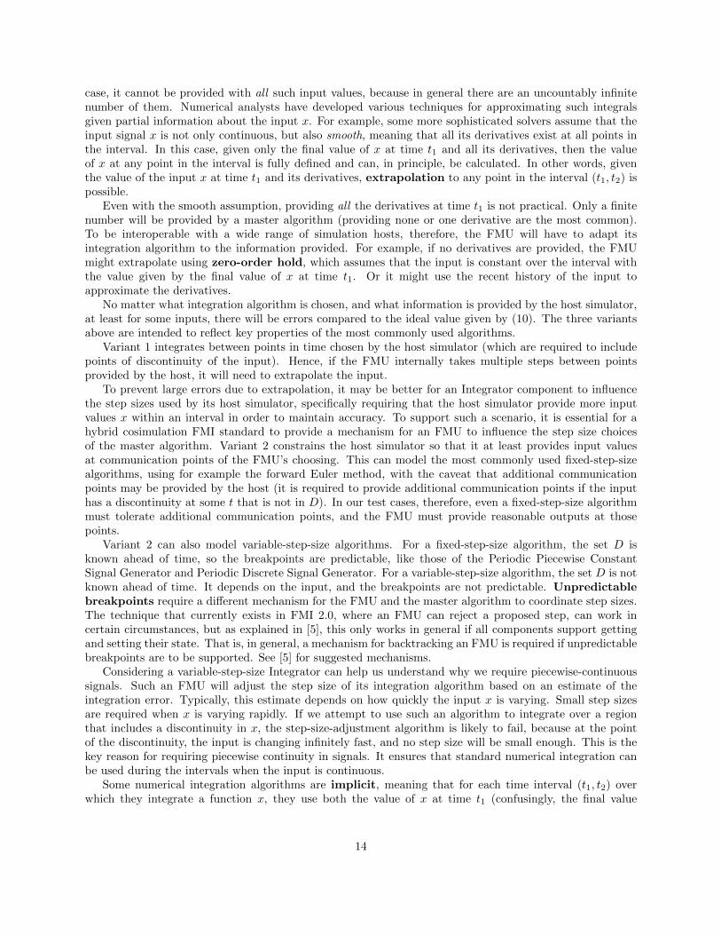
case, it cannot be provided with all such input values, because in general there are an uncountably infinitenumber of them. Numerical analysts have developed various techniques for approximating such integralsgiven partial information about the input x. For example, some more sophisticated solvers assume that theinput signal x is not only continuous, but also smooth, meaning that all its derivatives exist at all points inthe interval. In this case, given only the final value of x at time t1 and all its derivatives, then the valueof x at any point in the interval is fully defined and can, in principle, be calculated. In other words, giventhe value of the input x at time t1 and its derivatives, extrapolation to any point in the interval (t1, t2) ispossible.

Even with the smooth assumption, providing all the derivatives at time t1 is not practical. Only a finitenumber will be provided by a master algorithm (providing none or one derivative are the most common).To be interoperable with a wide range of simulation hosts, therefore, the FMU will have to adapt itsintegration algorithm to the information provided. For example, if no derivatives are provided, the FMUmight extrapolate using zero-order hold, which assumes that the input is constant over the interval withthe value given by the final value of x at time t1. Or it might use the recent history of the input toapproximate the derivatives.

No matter what integration algorithm is chosen, and what information is provided by the host simulator,at least for some inputs, there will be errors compared to the ideal value given by (10). The three variantsabove are intended to reflect key properties of the most commonly used algorithms.

Variant 1 integrates between points in time chosen by the host simulator (which are required to includepoints of discontinuity of the input). Hence, if the FMU internally takes multiple steps between pointsprovided by the host, it will need to extrapolate the input.

To prevent large errors due to extrapolation, it may be better for an Integrator component to influencethe step sizes used by its host simulator, specifically requiring that the host simulator provide more inputvalues x within an interval in order to maintain accuracy. To support such a scenario, it is essential for ahybrid cosimulation FMI standard to provide a mechanism for an FMU to influence the step size choicesof the master algorithm. Variant 2 constrains the host simulator so that it at least provides input valuesat communication points of the FMU’s choosing. This can model the most commonly used fixed-step-sizealgorithms, using for example the forward Euler method, with the caveat that additional communicationpoints may be provided by the host (it is required to provide additional communication points if the inputhas a discontinuity at some t that is not in D). In our test cases, therefore, even a fixed-step-size algorithmmust tolerate additional communication points, and the FMU must provide reasonable outputs at thosepoints.

Variant 2 can also model variable-step-size algorithms. For a fixed-step-size algorithm, the set D isknown ahead of time, so the breakpoints are predictable, like those of the Periodic Piecewise ConstantSignal Generator and Periodic Discrete Signal Generator. For a variable-step-size algorithm, the set D is notknown ahead of time. It depends on the input, and the breakpoints are not predictable. Unpredictablebreakpoints require a different mechanism for the FMU and the master algorithm to coordinate step sizes.The technique that currently exists in FMI 2.0, where an FMU can reject a proposed step, can work incertain circumstances, but as explained in [5], this only works in general if all components support gettingand setting their state. That is, in general, a mechanism for backtracking an FMU is required if unpredictablebreakpoints are to be supported. See [5] for suggested mechanisms.

Considering a variable-step-size Integrator can help us understand why we require piecewise-continuoussignals. Such an FMU will adjust the step size of its integration algorithm based on an estimate of theintegration error. Typically, this estimate depends on how quickly the input x is varying. Small step sizesare required when x is varying rapidly. If we attempt to use such an algorithm to integrate over a regionthat includes a discontinuity in x, the step-size-adjustment algorithm is likely to fail, because at the pointof the discontinuity, the input is changing infinitely fast, and no step size will be small enough. This is thekey reason for requiring piecewise continuity in signals. It ensures that standard numerical integration canbe used during the intervals when the input is continuous.

Some numerical integration algorithms are implicit, meaning that for each time interval (t1, t2) overwhich they integrate a function x, they use both the value of x at time t1 (confusingly, the final value

14

at that time) and the value of x at time t2 (confusingly, the initial value at that time). In this case,instead of extrapolating the input value, the numerical integrator interpolates the input. For example, thetrapezoidal method assumes that the input x varies linearly between t1 and t2, given only input valuesat t1 and t2.

Variant 3 supports implicit integration methods. However, as pointed out above, this variant makes theFMU strict, meaning that the output at any time t depends on the input at time t. Such a dependence is notpresent in the ideal definition of integration, given in (10). Use of such algorithms makes it more challengingto use such a component in a feedback loop, because such use could yield a causality loop.

3.9 Integrator with Reset

The output is the integral of the input, but an additional discrete input can reset the state of the integrator.


• DE input signal r;


Let D ⊂ T denote the set of time stamps (t, n) ∈ D where r(t, n) 6= ε. I.e., for all (t, n) ∈ T where (t, n) /∈ D,r(t, n) = ε. Since this set is order isomorphic with a subset of the natural numbers, we can list its elementsin order, d0, d1, d2, · · · , where dn < dn+1. For all (t, n) ∈ T , the output is defined to be

y(t, n) =

{ ∫ t

0x(α, 0)dα if (t, n) < d0 or D = ∅

r(d) +∫ t

ux(α, 0)dα otherwise

where d = (u,m) is the largest element in D s.t. (u,m) ≤ (t, n). We assume the same three variants as theIntegrator component, with the additional constraint that for all variants, there must be a communicationpoint at every (t, n) ∈ D. In addition, to ensure a piecewise-continuous output, for every (t, n) ∈ D, werequire a communication point at (t, 0).

Discussion. Absent any reset events r, this is identical to the Integrator above. At the time of resetevents, the state of the integrator (its output y) gets reset to the value of the reset event. Like the Integrator,the output y has no immediate dependence on the input x, and it does not depend on the value of the inputat non-zero microsteps (in the ideal). But the output y does immediately depend on the input r.

Assuming r is piecewise continuous, it is absent at all (t, 0). Reset events can only occur at microstepsgreater than zero. This ensures that the output y is piecewise continuous. Suppose a reset event occurs atsuperdense time (t1, 1). The output y(t1, 0) is unaffected by it, and hence is part of the preceding continuoussegment. At the next microstep, y(t1, 1) takes on the value given by r(t1, 1). If there are no further resetevents at time t1, then this will be the final value of the output, which provides the initial integrator statefor the next integration interval.

3.10 Zero-Crossing Detector

The output is a discrete event when the input hits or crosses zero.



For all (t, n) ∈ T , the output is

y(t, n) =

0 if x(t, 0) = 0, n = 1, and there exists a δ > 0 s.t.

for all 0 < ε < δ, x(t− ε, 0) 6= 00 if n > 0 and x(t, n− 1) and x(t, n) have opposite signs,0 if n > 0 and x(t, n− 1) 6= 0 and x(t, n) = 0,ε otherwise

(11)

To remove any ambiguity, “opposite signs” means that one value is negative, and the other value is positive.

15

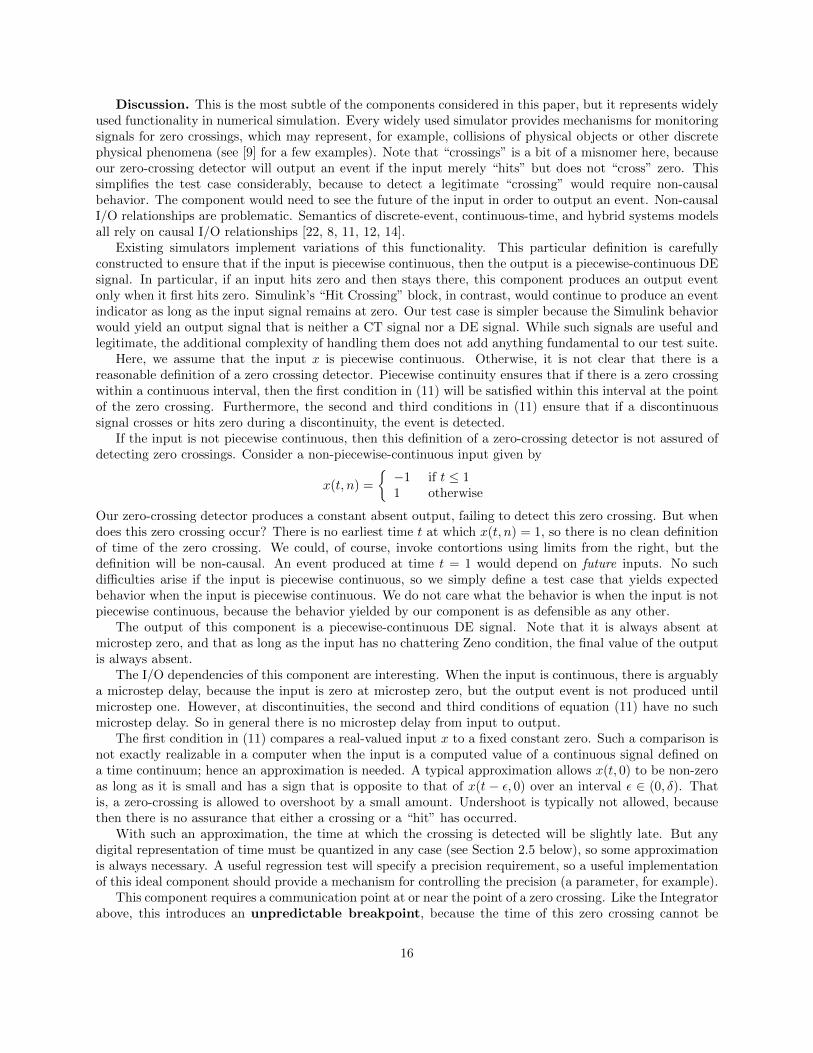
Discussion. This is the most subtle of the components considered in this paper, but it represents widelyused functionality in numerical simulation. Every widely used simulator provides mechanisms for monitoringsignals for zero crossings, which may represent, for example, collisions of physical objects or other discretephysical phenomena (see [9] for a few examples). Note that “crossings” is a bit of a misnomer here, becauseour zero-crossing detector will output an event if the input merely “hits” but does not “cross” zero. Thissimplifies the test case considerably, because to detect a legitimate “crossing” would require non-causalbehavior. The component would need to see the future of the input in order to output an event. Non-causalI/O relationships are problematic. Semantics of discrete-event, continuous-time, and hybrid systems modelsall rely on causal I/O relationships [22, 8, 11, 12, 14].

Existing simulators implement variations of this functionality. This particular definition is carefullyconstructed to ensure that if the input is piecewise continuous, then the output is a piecewise-continuous DEsignal. In particular, if an input hits zero and then stays there, this component produces an output eventonly when it first hits zero. Simulink’s “Hit Crossing” block, in contrast, would continue to produce an eventindicator as long as the input signal remains at zero. Our test case is simpler because the Simulink behaviorwould yield an output signal that is neither a CT signal nor a DE signal. While such signals are useful andlegitimate, the additional complexity of handling them does not add anything fundamental to our test suite.

Here, we assume that the input x is piecewise continuous. Otherwise, it is not clear that there is areasonable definition of a zero crossing detector. Piecewise continuity ensures that if there is a zero crossingwithin a continuous interval, then the first condition in (11) will be satisfied within this interval at the pointof the zero crossing. Furthermore, the second and third conditions in (11) ensure that if a discontinuoussignal crosses or hits zero during a discontinuity, the event is detected.

If the input is not piecewise continuous, then this definition of a zero-crossing detector is not assured ofdetecting zero crossings. Consider a non-piecewise-continuous input given by

x(t, n) =

{−1 if t ≤ 11 otherwise

Our zero-crossing detector produces a constant absent output, failing to detect this zero crossing. But whendoes this zero crossing occur? There is no earliest time t at which x(t, n) = 1, so there is no clean definitionof time of the zero crossing. We could, of course, invoke contortions using limits from the right, but thedefinition will be non-causal. An event produced at time t = 1 would depend on future inputs. No suchdifficulties arise if the input is piecewise continuous, so we simply define a test case that yields expectedbehavior when the input is piecewise continuous. We do not care what the behavior is when the input is notpiecewise continuous, because the behavior yielded by our component is as defensible as any other.

The output of this component is a piecewise-continuous DE signal. Note that it is always absent atmicrostep zero, and that as long as the input has no chattering Zeno condition, the final value of the outputis always absent.

The I/O dependencies of this component are interesting. When the input is continuous, there is arguablya microstep delay, because the input is zero at microstep zero, but the output event is not produced untilmicrostep one. However, at discontinuities, the second and third conditions of equation (11) have no suchmicrostep delay. So in general there is no microstep delay from input to output.

The first condition in (11) compares a real-valued input x to a fixed constant zero. Such a comparison isnot exactly realizable in a computer when the input is a computed value of a continuous signal defined ona time continuum; hence an approximation is needed. A typical approximation allows x(t, 0) to be non-zeroas long as it is small and has a sign that is opposite to that of x(t − ε, 0) over an interval ε ∈ (0, δ). Thatis, a zero-crossing is allowed to overshoot by a small amount. Undershoot is typically not allowed, becausethen there is no assurance that either a crossing or a “hit” has occurred.

With such an approximation, the time at which the crossing is detected will be slightly late. But anydigital representation of time must be quantized in any case (see Section 2.5 below), so some approximationis always necessary. A useful regression test will specify a precision requirement, so a useful implementationof this ideal component should provide a mechanism for controlling the precision (a parameter, for example).

This component requires a communication point at or near the point of a zero crossing. Like the Integratorabove, this introduces an unpredictable breakpoint, because the time of this zero crossing cannot be

16

known in advance, in general. A typical realization of such a Zero-Crossing Detector cooperates with themaster algorithm to regulate the step size taken by a simulator so that the detection delay is less thansome specified time resolution. As a consequence, a hybrid cosimulation FMI standard should include amechanism for an FMU to cooperate with the host simulator, regulating time steps taken by the simulator.One mechanism would be for the FMU to be able to reject step sizes proposed by the host simulator untilthe step size is small enough to detect the zero crossing within the specified resolution. Again, see [5] for adiscussion of such mechanisms.

When an FMU rejects a step size because a zero crossing has occurred, it may be able to estimate thetime at which the zero crossing actually occurs by interpolating between the specified inputs. Hence, forefficiency, a hybrid cosimulation standard should also include a mechanism for an FMU to be able to suggesta better step size when it rejects one.

Note that it appears that a reasonable approximation of a zero-crossing detector is difficult using FMI 2.0for cosimulation as defined in [16]. In particular, when advancing time using fmi2DoStep, the host simulatorprovides no information about the value of the inputs at the end of the step. Hence, the FMU cannot rejecta step size proposed by fmi2DoStep. The API does provide a way to reject a setting of input values usingfmi2SetReal (which can return fmi2Discard). But almost certainly this is not intended to be used to rejecta previously accepted step size and trigger a redoing of the step.

This component can only be approximated in FMI 2.0 for cosimulation by extrapolating the input, usingthe derivatives of the input, if provided, or an extrapolation based on the history of the input.

3.11 Zero-Order Hold



The output is defined to be

y(τ) =

{x(d) if d exists,ε otherwise

where d is the largest element in T s.t. d ≤ τ and x(d) 6= ε.Discussion. Recall that a DE signal is non-absent at a discrete subset of times. This property ensures

that if there is any input event at all, then all outputs at the time of that event and beyond are not absent.Specifically, if there is any time τ0 ∈ T where x(τ0) 6= ε, then for all τ ∈ T where τ ≥ τ0, there exists alargest d ≤ τ such that x(d) 6= ε.

If the input is piecewise continuous, then the output will also be piecewise continuous. This fact is notentirely obvious from the definition. Note that for x to be a piecewise-continuous DE signal, it must be truethat both its initial and final value functions are absent. Hence, if an event arrives on x at time t0 ∈ R+,then the event must occur at a microstep strictly greater than 0. That is, x(t0, 0) = ε. Hence, y(t0, 0)will have the value specified by previous event (or be absent if there is no previous event). Suppose thatx(t0, 1) 6= ε. Then y(t0, 1) = x(t0, 1). If final value of x at t0 is x(t0, 2) = ε, then the final value of y at t0will be y(t0, 1) = x(t0, 1), and this will be the value of y until (and including) (t1, 0), where t1 is the time ofthe arrival of the next event.

The output of this component has a discontinuity at each time t where x(t, n) 6= ε. In order for thisdiscontinuity to manifest correctly as a sequence of two distinct values at the same time t with distinctmicrosteps, there will need to be two distinct communication points at the time t of the input event. Supposethat an input event occurs at (t, n) for some n > 0. That is, x(t, n) 6= ε. It is sufficient for the host simulatorto provide a communication point at both (t, 0) and (t, n). But to provide a communication point at (t, 0),the host simulator needs to “anticipate” the event at (t, n). This seems to imply non-causal behavior.

Fortunately, we can meet this requirement without any non-causal mechanisms. The simplest mechanismis already realized in FMI 2.0, where whenever a non-zero step size is taken, the next communication pointautomatically occurs at microstep zero. There is no mechanism in FMI 2.0 to skip microstep zero. ThePtolemy II Continuous director [18], which implements hybrid system simulation, also always provides a

17

communication point (t, 0) for every communication point (t, n). So a Zero-Order Hold FMU will never beforced to reject a time step if Ptolemy II is the host simulator.

But even if the future hybrid cosimulation standard does provide a mechanism to advance from communi-cation point (t0, n0) to (t1, n1), where t1 > t0 and n1 > 0, then an FMU implementing this Zero-Order Holdcomponent can reject the proposed step. It thereby ensures that for every communication point (t, n), therewill also be a communication point (t, 0). This mechanism does not require anticipating future events.

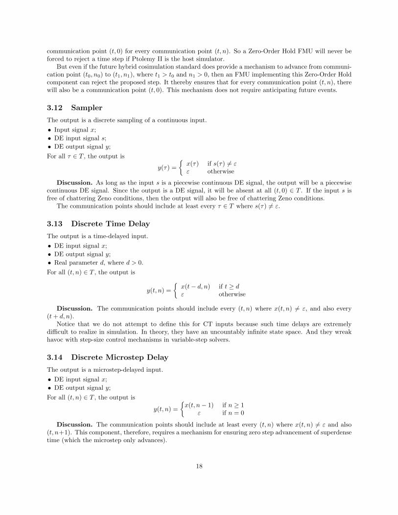
3.12 Sampler

The output is a discrete sampling of a continuous input.

• Input signal x;

• DE input signal s;


For all τ ∈ T , the output is

y(τ) =

{x(τ) if s(τ) 6= εε otherwise

Discussion. As long as the input s is a piecewise continuous DE signal, the output will be a piecewisecontinuous DE signal. Since the output is a DE signal, it will be absent at all (t, 0) ∈ T . If the input s isfree of chattering Zeno conditions, then the output will also be free of chattering Zeno conditions.

The communication points should include at least every τ ∈ T where s(τ) 6= ε.

3.13 Discrete Time Delay

The output is a time-delayed input.



• Real parameter d, where d > 0.


y(t, n) =

{x(t− d, n) if t ≥ dε otherwise

Discussion. The communication points should include every (t, n) where x(t, n) 6= ε, and also every(t+ d, n).

Notice that we do not attempt to define this for CT inputs because such time delays are extremelydifficult to realize in simulation. In theory, they have an uncountably infinite state space. And they wreakhavoc with step-size control mechanisms in variable-step solvers.

3.14 Discrete Microstep Delay

The output is a microstep-delayed input.




y(t, n) =

{x(t, n− 1) if n ≥ 1

ε if n = 0

Discussion. The communication points should include at least every (t, n) where x(t, n) 6= ε and also(t, n+1). This component, therefore, requires a mechanism for ensuring zero step advancement of superdensetime (which the microstep only advances).

18

Notice that we do not attempt to define this for CT inputs. Indeed, if presented with a CT input, thiscomponent will produce a rather odd output signal, one whose initial value is always absent, and subsequentvalues are present. If the input is a piecewise continuous DE signal, then the input is always absent atmicrostep zero, and the output will also be piecewise continuous. If the input is free of chattering Zenoconditions, then the output will be free of chattering Zeno conditions. In this case, the final value of theinput is also ε, so the final value of the output will be ε.

Notice further that we do not generalize this component to have a parameter m to delay by m microsteps.See the discussion in Section 4.4 below for the reason for this.

4 Composition Test Cases

A hybrid cosimulation FMI standard that enables definition of the above components provides a rich frame-work for composition of discrete and continuous simulation tools. Any such standard should be able tounambiguously define FMUs that realize such components and should ensure that host simulators are capa-ble of executing these FMUs. Such capabilities can be verified using unit tests that check each of the abovecomponents individually by providing a range of inputs and verifying that the outputs match the ideal (upto some precision, where appropriate). But such unit tests are not quite sufficient. We also need to ensurethat interactions between multiple components behave correctly.

In this section, we discuss some test cases that combine a few of the above components, and give accep-tance criteria that define correct behavior. These test cases are, in effect, constraints on master algorithms.Host simulators that conform with the standard must implement master algorithms that satisfy these ac-ceptance criteria.

4.1 Synchronous Events

This test case checks that multiple components with discrete timed behavior coordinate their representationsof time. Consider the composition shown in Figure 4. This has three components:

1. A Periodic Discrete Signal Generator with period p=1/3 and a=1.

2. A Periodic Discrete Signal Generator with period p=2/3 and a=1.

3. A Sampler with DE input x

The test criterion is that the output of the Sampler should equal the output of second Periodic DiscreteSignal Generator at all superdense times. More generally, we would like the periods to be p = q and 2q,where q is a representable time, given as 1/3 in our test case.

Discussion. FMUs may internally use representations of time that are different from that of the hostsimulator. This test criterion is intended to ensure that no matter how the FMU and host simulatorinternally represent time, the Sampler and Periodic Discrete Signal Generator semantics are respected. Thistest case also checks for a well-defined notion of simultaneity. In particular, the periods chosen are not

Figure 4: Test case for sampling of discrete event signals.

19

exactly representable with double precision floating point numbers, and the test is intended to ensure thatdespite any roundoff errors, every second output of the first Periodic Discrete Signal Generator is exactlysynchronous with every output of the second one. The Test component must see the events at the samecommunication point in superdense time.

4.2 Integrating Discontinuous Signals

Figure 5 shows a test case that integrates a discontinuous input. The output is continuous, and shouldmatch Figure 6. Every acceptable test result will produce at least one output sample at the times of thediscontinuities of the output of the Periodic Piecewise Constant Signal Generator. Samples in between thesepoints in time are optional, and may depend on the step-size control algorithm used by the host simulator.

Discussion. The key feature being tested here is that a host simulator does not get confused by a signalthat has two distinct values at the same (real) time, at distinct microsteps, and that a sequence of valuesat a (real) time does not affect the output of an Integrator, except that the final value at a discontinuitybecomes the initial value for the next integration interval.

4.3 Integrating Glitches

Figure 7 shows a test case that verifies that the Integrator output is unaffected by input values whoseduration is zero. In this test case, a constant-valued signal is modified using an Adder so that its value atinteger-valued times sequences from 1 to 2 and back to 1, without time elapsing. These glitches have zerowidth, and hence should not affect the output of the Integrator.

4.4 Zero-Delay Feedback

Figure 8 shows a test model using a Zero-Crossing Detector in a feedback loop. The Integrator with Resetis integrating a constant 1, and hence will produce a line with unit slope. When that line crosses 1, theZero-Crossing Detector is triggered. The event it produces is fed back through a Discrete Microstep Delayand through a Triggered Constant, which provides a discrete event with value 0 to the reset input of theIntegrator with Reset.

The expected output is shown in Figure 9. Because of the approximate nature of the Zero-CrossingDetector (see Section 3.10), the times at which the reset occurs and the value at which it is triggered areapproximate, so a regression test needs to specify a tolerance.

Figure 5: Test case for integrating discontinuous inputs.

y(t, n)

t

1

00 1 2 3

Figure 6: Result of the composition of components shown in Figure 5. The dots show required samples.

20

Figure 7: Test case for integrating glitches.

Figure 8: Test case for zero-delay feedback. The required output is shown in Figure 9.

y(t, n)

t

1

00 1 2 3

Figure 9: Required output from the test model in Figure 8. The unfilled dots show values that occur onlyat microsteps n ≥ 2, whereas the filled dots and lines show values at n = 0 and n = 1.

21

In the plot in Figure 9, the filled and unfilled dots are required samples, occurring at microsteps 0 and2 respectively. Samples in between are optional and may depend on the step-size control algorithm of thehost simulator. Specifically, at time t = 1, the output of the Integrator With Reset should be

y(1, 0) = a

y(1, 1) = a

y(1, 2) = 0

where a ≈ 1.Notice that the reset actually occurs in microstep 2, because the event at the output of the Zero-Crossing

Detector occurs at microstep 1, and it is then delayed by one additional microstep. In this particular instance,the Discrete Microstep Delay in the feedback loop might not seem to be required because the input to theZero-Crossing Detector is continuous, and by the definition of the Zero-Crossing Detector, it introduces amicrostep delay when the zero crossing occurs in a continuous region of the input. Nevertheless, our testcase includes a Discrete Microstep Delay for two reasons. First, it provides a test where microsteps explicitlygo beyond 1. Second, the Zero-Crossing Detector introduces a microstep delay only for some inputs. Sothe presence of a microstep delay in the loop is not a static property, which complicates scheduling of thecomponents. Specifically, the Discrete Microstep Delay is non-strict, meaning that its input at superdensetime τ need not be known to retrieve its output at τ . A scheduler can take this into account to break theapparent dependency loop created by the feedback. The Zero-Crossing Detector, however, is only non-strictat microstep zero (because its output is always absent at microstep zero). Hence, without the DiscreteMicrostep Delay, we would have a causality loop at all microsteps but zero. A master algorithm would haveto ensure that at the input to the Zero-Crossing Detector, mt = 0 for all t. In general, this is difficult toensure.

Discussion. A subtle point raised by this composition is that the master algorithm needs to “know”at any time t when all signals have reached their final microstep. Specifically, it is not sufficient to stopincrementing microsteps at time t when all signals become absent at time t. First, CT signals never becomeabsent at time t, so the mere presence of a CT signal will foil this strategy. Second, the Discrete MicrostepDelay may have an absent input, and yet, in the next microstep, produce a non-absent output.

Our assumption is that each FMU constrains step sizes so that prior to reaching the final microstep ofits outputs, it prevents the master algorithm from advancing time. It only permits advances in microstep.When no component does this, the master algorithm can assume that all signals have reached their finalmicrostep.

For simplicity, we have constrained Discrete Microstep Delay so that it can only produce a non-absentoutput at the very next microstep. I.e., it implements a unit microstep delay, not an m-step microstepdelay. It is certainly possible to generalize this mechanism to allow an m-step microstep delay, but we havenot encountered any need for such generality, so we have not included this in the test cases for a hybridcosimulation standard.

The Discrete Microstep Delay, the Discrete Time Delay, and both Integrator components have the prop-erty that they prevent causality loops when forming feedback compositions.2 Specifically, these componentshave the unique property that they are able to produce outputs at a superdense time τ without any knowl-edge of their input values at τ . Such components are said to be non-strict. The Integrator with Reset isnon-strict only with respect to the x input. It is strict with respect to the r input. Hence, strictness is arelation between input and output ports, and not a property of a component. This relationship needs tobe declared as a static interface property of a component, so that a master algorithm can analyze causalityproperties, check models for constructiveness (see [9]), and optimize the schedule of invocation of FMUs.The FMI 2.0 specification supports an optional element for specifying such dependencies between input andoutput ports. For a detailed discussion of such causality relations, see [23].

2This assumes the Integrators implement variants 1 or 2, using an explicit integration method.

22

Figure 10: Test case verifying that various ways of producing piecewise-constant signals produce identicalsignals. The required output is shown in Figure 1.

4.5 Piecewise Constant Signals

The test components given in Section 3 offer a number of ways to construct the piecewise-constant signal inFigure 1. The model in Figure 10 tests that these various ways produce identical signals.

5 Conclusion

Hybrid cosimulation is a far from trivial goal. A standard that enables composition of simulation tools hastwo conflicting objectives. It needs to be sufficiently rigorous to define the meaning of a composition ofcomponents. And it needs to be flexible enough to embrace industry-standard and established simulators.The former demands a rigorous semantics, but the later creates pressure for less well-defined semantics.

This paper does not define such a standard, but instead enumerates a set of capabilities that such astandard must support to be useful. In particular, the paper enumerates a suite of components and testcases that cover a wide range of hybrid system behaviors. We have attempted to keep the components assimple as possible, but some cases, “as simple as possible” is not very simple. The most complex of thecomponents are the Integrators, the Zero-Crossing Detector, and the Modal Models, which, although theyrepresent widely used functionality in hybrid system simulation, have subtle properties.

The components defined in this paper are meant to be test cases, not library components. In most cases,to be useful in a library of components, they would need to be further generalized and parameterized. Forexample, the Zero-Crossing Detector would probably have a parameter that would specify whether upwards,downwards, or both directions of crossing are of interest. It could also have another parameter for a levelcrossing other than zero to detect. While such enhancements would increase the utility of the components,they do not enhance their value as test cases.

The following features, at least, are captured by the test cases:

1. A component may have zero latency from an input to an output.

2. A component can output discontinuous signals, and so that those signals are compatible with integrationalgorithms, they are piecewise continuous.

3. A component can reject step sizes based on internal accuracy estimates of numerical integration.

4. A component can reject step sizes in order to ensure that the simulation does not step over or skip a timeat which a discrete event occurs.

23

5. A component can reject step sizes and suggest better step sizes in order to approximate event detection(such as zero crossings).

6. A component can react to DE inputs and produce DE outputs.

7. A component that reacts to DE inputs and produces continuous outputs produces piecewise-continuousoutputs.

8. Discontinuities in signals can be exactly represented by samples of the signal, thanks to superdense time.

9. A component can monitor a continuous input and produce discrete events when some condition is detected,such as a zero-crossing.

References

[1] R. Alur, C. Courcoubetis, N. Halbwachs, T. Henzinger, P. Ho, X. Nicollin, A. Olivero, J. Sifakis, and S. Yovine.The algorithmic analysis of hybrid systems. Theoretical Computer Science, 138:3–34, 1995.

[2] R. Alur and D. L. Dill. A theory of timed automata. Theoretical Computer Science, 126(2):183–235, 1994.

[3] A. Benveniste and G. Berry. The synchronous approach to reactive and real-time systems. Proceedings of theIEEE, 79(9):1270–1282, 1991.

[4] T. Blochwitz, M. Otter, M. Arnold, C. Bausch, C. Clauß, H. Elmqvist, A. Junghanns, J. Mauss, M. Monteiro,T. Neidhold, D. Neumerkel, H. Olsson, J.-V. Peetz, and S. Wolf. The functional mockup interface for toolindependent exchange of simulation models. In Proc. of the 8-th International Modelica Conference, Dresden,Germany, Mar. 2011. Modelica Association.

[5] D. Broman, C. Brooks, L. Greenberg, E. A. Lee, M. Masin, S. Tripakis, and M. Wetter. Determinate Compositionof FMUs for Co-Simulation. In Proceedings of the International Conference on Embedded Software (EMSOFT2013). IEEE, 2013.

[6] L. P. Carloni, R. Passerone, A. Pinto, and A. Sangiovanni-Vincentelli. Languages and tools for hybrid systemsdesign. Foundations and Trends in Electronic Design Automation, 1(1/2), 2006.

[7] D. Harel and A. Pnueli. On the development of reactive systems. In K. R. Apt, editor, Logic and Modelsfor Verification and Specification of Concurrent Systems, volume F13 of NATO ASI Series, pages 477–498.Springer-Verlag, 1985.

[8] E. A. Lee. Modeling concurrent real-time processes using discrete events. Annals of Software Engineering,7:25–45, 1999.

[9] E. A. Lee. Constructive models of discrete and continuous physical phenomena. IEEE Access, 2(1):1–25, 2014.

[10] E. A. Lee and A. Sangiovanni-Vincentelli. A framework for comparing models of computation. IEEE Transactionson Computer-Aided Design of Circuits and Systems, 17(12):1217–1229, 1998.

[11] E. A. Lee and H. Zheng. Operational semantics of hybrid systems. In M. Morari and L. Thiele, editors,Hybrid Systems: Computation and Control (HSCC), volume LNCS 3414, pages 25–53, Zurich, Switzerland,2005. Springer-Verlag.

[12] X. Liu, E. Matsikoudis, and E. A. Lee. Modeling timed concurrent systems. In CONCUR 2006 - ConcurrencyTheory, volume LNCS 4137, pages 1–15, Bonn, Germany, 2006. Springer.

[13] O. Maler, Z. Manna, and A. Pnueli. From timed to hybrid systems. In Real-Time: Theory and Practice, REXWorkshop, pages 447–484. Springer-Verlag, 1992.

[14] E. Matsikoudis and E. A. Lee. On fixed points of strictly causal functions. In International Conference onFormal Modeling and Analysis of Timed Systems (FORMATS), volume LNCS 8053, pages 183–197. Springer-Verlag, 2013.

[15] Modelica Association. Modelica textregistered - a unified object-oriented language for physical systems modeling:Language specification version 3.1. Report, May 27 2009.

[16] Modelica Association. Functional mock-up interface for model exchange and co-simulation. Report 2.0, July 252014.

[17] M. Otter, M. Malmheden, H. Elmqvist, S. E. Mattsson, and C. Johnsson. A new formalism for modeling ofreactive and hybrid systems. In Modelica Conference. The Modelica Association, 2009.

24

[18] C. Ptolemaeus, editor. System Design, Modeling, and Simulation using Ptolemy II. Ptolemy.org, Berkeley, CA,2014.

[19] P. Tabuada. Verification and Control of Hybrid Systems: A Symbolic Approach. Springer, 2009.

[20] M. M. Tiller. Introduction to Physical Modeling with Modelica. Kluwer Academic Publishers, 2001.

[21] S. Tripakis and D. Broman. Bridging the Semantic Gap Between Heterogeneous Modeling Formalisms and FMI.Technical Report UCB/EECS-2014-30, EECS Department, University of California, Berkeley, Apr 2014.

[22] B. P. Zeigler, H. Praehofer, and T. G. Kim. Theory of Modeling and Simulation. Academic Press, 2nd edition,2000.

[23] Y. Zhou and E. A. Lee. Causality interfaces for actor networks. ACM Transactions on Embedded ComputingSystems (TECS), 7(3):1–35, 2008.

25

Requirements for Hybrid Cosimulation - Simulation...

Documents

Transcript of Requirements for Hybrid Cosimulation - Simulation...