1

Reputation Effects of Disclosure*, **

Radhika Lunawat

†

July 2010

*This paper is based on my Ph.D. dissertation at University of Minnesota. I am indebted to my

dissertation committee for the valuable suggestions and guidance: John Dickhaut (Chair), Beth

Allen, Chandra Kanodia and Greg Waymire. I wish to thank Ron King, Christian Leuz, Harry

Evans, Gord Richardson and Jack Stecher for helpful comments and suggestions. I also wish to

thank conference participants at 2007 Economic Science Association North American meeting,

Vernon Smith Conference 2007, European Accounting Association 24th Doctoral Colloquium in

Accounting, Spring 2008 Midwest Economic Theory Conference, Econometric Society North

American Summer Meeting 2008, 2008 International Economic Science Association Conference,

American Accounting Association Annual Meeting 2008 and 2009 International Economic

Science Association Conference; workshop participants at London School of Economics, Indian

School of Business, University of Pittsburgh, Chapman University, University of Toronto and

University of Alberta; referees for National Science Foundation Doctoral Dissertation Grant and

referees for University of Minnesota Graduate School Fellowship.

**I gratefully acknowledge support from National Science Foundation Doctoral Dissertation

Grant Number 0820455 and from Accounting Research Center at Carlson School of

Management, University of Minnesota.

†Department of Accounting, Opus College of Business, University of St Thomas, 1000 LaSalle

Avenue, Mail# TMH 443, Minneapolis, MN 55403; e-mail: rlunawat@stthomas.edu.

2

Abstract

This paper analyzes the role of disclosure in building reputation for being trustworthy. I

allow for information asymmetry in a finitely repeated sender-receiver game and solve

for sequential equilibrium to show that if there are some trustworthy managers who

always disclose their private information (or there is simply a belief that there are some

trustworthy managers), then a rational manager will choose to disclose her private

information in an attempt to earn a reputation for being trustworthy. However, except

under certain circumstances, the rational manager will switch from mimicking to be the

trustworthy manager with probability one to mimicking to be the trustworthy manager

with a certain probability strictly less than one. I define two regimes, in both of which

there is information asymmetry but only one allows for disclosure in the form of

communication of private information. I show that the regime with disclosure allows for

a greater time of mimicking with probability one and this additional reputation building

opportunity results in higher probability of investment and higher probability of high

returns on investment. I also show that a manager will prefer the regime without

disclosure while an investor will prefer the regime with disclosure.

Keywords. Disclosure, Reputation, Investment, Trust.

3

1. Introduction

“In the United States, home to some of the largest corporate collapses, trust in business

collapsed as well, dropping 20 percentage points over the course of one year. With only

38% of informed public in the United States trusting business today, levels are the lowest

they have been in the Barometer‟s tracking history – even lower than in the wake of

Enron and the dot-com bust…For U.S. businesses, this downturn marks a stark reversal

from the steady uptick in trust of the last five years….”

– Edelman Trust Barometer 2009

“Something important was destroyed in the last few months. It is an asset crucial to

production…. While this asset does not enter standard national account statistics or

standard economic models, it is so crucial to development that its absence – according to

Nobel laureate Kenneth Arrow – is the cause of much of the economic backwardness in

the world. This asset is TRUST….Without trust, co-operation breaks down, financing

breaks down and investment stops. One can bomb a country back to the Stone Age,

destroy much of its human capital, and eliminate its political institution. But, if trust

persists, the country may be able to right itself in just a few years, as in Germany and

Japan after World War II. Conversely, you can endow a country with all the greatest

natural resources but if there is no trust, there is no progress.”

– Sapienza and Zingales, 2009

In the backdrop of the financial meltdown, trust and corporate reputation have been a

huge casualty. As businesses launch what print media refers to as the “Great Trust

Offensive (BusinessWeek, Sept 28th

2009)” to reclaim their lost trust and reputation in a

bid to win back consumer confidence, a natural question that arises is the role financial

disclosure may play in facilitating this trust. Extant literature in accounting attributes to

financial disclosure a role in reducing the information asymmetry component of cost of

capital (Verrecchia, 2001 and Dye, 2001). Another strand of literature explicates the role

4

financial disclosure plays in real investment and managerial decisions of a firm (Kanodia,

2006). This work establishes an additional role of financial disclosure, namely that of

building reputation for being trustworthy.

While anecdotally it seems that voluntary disclosure should provide opportunities for

reputation building, there are subtleties in the relation between disclosure and reputation

that are not so obvious. For example, I show that full disclosure will be sub-optimal and

that a rational manager will (except under certain specific circumstances) choose full

disclosure with a certain probability strictly less than one in order to ensure credibility of

her disclosure in instances where she chooses to disclose. The only exception will be

where the investor‟s belief about a manager‟s trustworthiness is exceptionally high and

then the manager will choose full disclosure to maintain the belief at that high level.

I examine the reputation building role of disclosure in a sender–receiver game, where the

sender / investor is endowed with some wealth and chooses whether or not to invest it in

a receiver / manager. The receiver is endowed with some production technology because

of which she channels the investment to productive uses. Depending on the state of

nature that obtains, the production may lead to a high or low yield. The manager may be

trustworthy or untrustworthy. A trustworthy manager will choose to share a fair

proportion of the yield with the investor whereas an untrustworthy manager‟s action will

be guided by her self-interest. This game is repeated finitely to allow for reputation

building.

I define two regimes, namely disclosure regime and no disclosure regime. In both

regimes, the manager learns the state of nature but the investor does not. However, in the

disclosure regime, the manager is allowed to share her private knowledge of the state of

nature with the investor. The finitely repeated nature of the game in both regimes allows

for reputation building. I solve for a sequential equilibrium in both regimes and examine

5

whether the ability to disclose private information provides reputation building

opportunities over and above those provided by the institution of dividend payment.

A question that arises is whether additional reputation building opportunities provided by

disclosure will result in higher investment and higher return in economies. This paper

sheds light on that question by comparing the probability of investment and the

probability of high returns on investment in the disclosure and no disclosure regimes.

While disclosure may result in higher investment and higher return on investment and

may therefore be socially optimal, do a manager and an investor both benefit from higher

disclosure? That is, given a choice will a manager opt for higher disclosure and will an

investor want her to do so? This paper examines the question by comparing an investor‟s

and a manager‟s payoffs in the disclosure and no disclosure regimes.

The sender-receiver game I define derives from the “investment game” first studied

experimentally in Berg, Dickhaut and McCabe, 1995. In this investment game a sender is

endowed with 10 units of wealth and decides how much of this endowment to send to a

receiver. The amount sent by the sender is tripled before it reaches the receiver. The

receiver decides how much of this tripled amount to keep and how much to send back.

Additionally, Dickhaut, Hubbard, Lunawat and McCabe, 2008 study a repeated

investment game where subjects play the investment game for 2 periods. Both studies

find evidence of trust, but trust is enhanced when the game is repeated. Specifically,

Dickhaut et al find that the amount returned by the receiver in period 1 is significantly

larger than the amount returned by the receiver in period 2, suggesting that in period 1

rational agents try to develop a reputation for being altruistic or trustworthy. Dickhaut,

Lunawat, Waymire and Xin, 2008 take the repeated investment game setting and replace

the multiplier of 3 by a stochastic multiplier. The receiver learns the multiplier but the

sender does not allowing for a definition of income (It is the amount received by the

receiver before sending something back) in their setting. They examine the relation of

6

disclosure and non-enforceable contract formation in single-venture settings and compare

the results as an economy grows in size and complexity. The question that remains open

is of the relation between disclosure and reputation and this works sheds light on that

relation.

While the setting derives from the investment game, the equilibrium solution derives

from Kreps and Wilson, 1982 and Kreps, Milgrom, Roberts and Wilson, 1982. Kreps and

Wilson, 1982 solve a sequential equilibrium for a monopolist entry deterrence game and

formally establish the role of reputation in a finitely repeated entry-deterrence game.

Kreps, Milgrom, Roberts and Wilson, 1982 solve for a sequential equilibrium in a finitely

repeated prisoners‟ dilemma game. Given the complexity of the equilibrium, Camerer

and Weigelt, 1988 play the lender-borrower game in a laboratory setting and find

experimental evidence supportive of sequential equilibrium. I solve for a sequential

equilibrium in both the disclosure and the no disclosure regimes.

The rest of the paper proceeds as follows. Sections 2 reviews related literature. Sections 3

and 4 respectively define the disclosure and no disclosure regimes and solve for

sequential equilibrium in respective regimes. Section 5 compares investment, return and

payoffs in the two regimes. Section 6 summarizes and concludes.

2. Literature Review

This paper contributes to the emerging literature looking at the very foundational issues

in accounting. Basu, Dickhaut, Hecht, Towry and Waymire, 2009 tests the evolutionary

hypothesis developed in Basu and Waymire, 2006 to provide evidence of the role of

financial recordkeeping in promoting trade and exchange. Jamal, Maier and Sunder, 2005

contrast the role of voluntary disclosure as a social norm with enforced standards and

conventions. This work explores foundational issues regarding the relation between

reputation and financial disclosure.

7

Theoretically, voluntary disclosure has been shown to occur because it is in the best

interest of rational agents (e.g. Grossman, 1981 and Dye, 1985a ). Disclosure has also

been shown to have a co-ordination role in an economy where higher-order beliefs are

crucial (Morris and Shin, 2002 and Angeletos and Pavan, 2004). This paper considers a

model of reputation formation under different institutional structures of disclosure to

show that voluntary disclosure occurs because rational self-interested agents have an

incentive to look like altruistic or trustworthy agents.

This paper is related to the strand of literature that looks at the different roles played by

disclosure. That literature has been surveyed by Healy and Palepu, 2001; Bushman and

Smith, 2001; and Leuz and Wysocki, 2008. Healy and Palepu, 2001 discuss several

motives for voluntary disclosure including its role in reducing cost of capital, in reducing

the likelihood of undervaluation, in avoiding litigation, in signaling managerial talent and

in lowering the cost of private information acquisition. It is also used strategically by

managers in receipt of stock-based compensation. Bushman and Smith, 2001 discuss

several channels through which financial accounting information affects economic

performance. It leads to better project identification, better governance and mitigates

adverse selection. Leuz and Wysocki, 2008 discuss the economic costs and benefits of

disclosure.

Arrow, 1972; Putnam, 1993; Fukuyama, 1995 and Solow, 1995 have written about the

effects of trust on economic activity. The question has been studied empirically by La

Porta, Lopez de Silanes, Shleifer and Vishny, 1997; Knack and Keefer, 1997; and Guiso,

Sapienza and Zingales, 2004 among others. However, the role of disclosure in facilitating

trust and thereby stimulating economic activity has not been analyzed and this paper

sheds light on that question.

Reputation for truthful reporting has been studied experimentally (e.g. King, 1996) and

reputation for informative reporting has been studied using archival data (e.g. Healy and

8

Palepu, 1993). The role of information disclosure in markets has been examined

experimentally in the context of market efficiency studies (e.g. Bloomfield, 1996 and

Bloomfield and Libby, 1996) and game-theoretic strategic disclosures (e.g. King and

Wallin, 1991, 1995). The role of information reporting or disclosure in developing

reputation for being trustworthy has not been studied and this paper sheds light on this

role.

Trust has been shown to induce reciprocity (e.g. Berg, Dickhaut and McCabe, 1995) and

foster economic exchange. The role of reputation versus reciprocity in repeated

interactions has been explored (e.g. McCabe, Rassenti and Smith, 1996). While these

questions have mostly been examined using behavioral theories and human subjects

experiments, at a theoretical level, trust has been conceptualized as a strategic attempt to

build reputation in a repeated game (e.g. Kreps, Milgrom, Roberts and Wilson, 1982).

Dickhaut, Hubbard, Lunawat and McCabe, 2009 explicitly model reputation for being

trustworthy while this paper introduces information asymmetry in the model to examine

the role of disclosure in building reputation for being trustworthy.

Berg, Dickhaut and McCabe, 1995 use the amount invested by the sender as a measure of

trust the sender has in the receiver. The efficacy of this measure in studying trust using

the World Values Survey is explored by Glaeser, Laibson, Scheinkman and Soutter,

2000. Sapienza, Toldra and Zingales, 2007 proposes the sender‟s expectation of the

receiver‟s behavior as a measure of trust and studies the efficacy of their measure in

studying trust using the World Values Survey. This paper shows that both the amount

invested by the sender and the sender‟s expectation of the receiver‟s behavior are higher

in the disclosure regime compared to the no disclosure regime.

3. Disclosure Regime

There are two players, A (sender / investor) and B (receiver / manager). Nature moves

first and selects B‟s type to be either trustworthy or untrustworthy. I will define

9

momentarily what I mean by each type. B knows her type but A does not. The game then

proceeds through n periods in each of which the A and B make a sequence of choices. In

what follows, the subscript t (t = 1, 2, …. , n) will be used to denote a period. B chooses

whether or not to disclose private information she will learn in the course of the game. A

decision to disclose is denoted by dt = 1 and a decision not to disclose is denoted by dt =

0. Note that B is not privy to the private information at the time she makes the choice of

whether or not to disclose it. It is information she will learn in the course of the game. It

is as if B is making a choice of an accounting system – B could choose an accounting

system that will generate information that both A and B will learn (by choosing to

disclose) or alternatively, B could choose an accounting system that will generate

information only B will learn (by choosing not to disclose).

A sees B‟s disclosure decision, is endowed with e > 0 units of wealth and chooses

whether or not to invest in B. Regardless of whether or not A chooses to invest, e is

common knowledge. That is, both A and B know the amount of wealth A in endowed

with. A‟s decision to invest is denoted by mt = e and A‟s decision not to invest is denoted

by mt = 0. If A chooses to invest, then the amount e is multiplied by a multiplier λt before

B receives it. λt {l, h} and is equally likely to be either l or h in every period. 1 ≤ l < 2

< h, l + h > 4.

Now B receives et and learns t. However, A learns λt only if B had earlier chosen to

disclose her private information. That is, if B had chosen an accounting system that

generates information both A and B learn, then A learns λt. Otherwise, if B had chosen an

accounting system that generates information only B learns, then A does not learn λt. In

this sense, λt is B‟s private information – she always learns the realized value of λt but

A‟s knowledge of λt is dependent on B‟s choice of accounting system.

After B receives et, she chooses to send back kt to B. If t = l, kt {0, el / 2}. If t = h,

kt {0, el / 2, eh / 2}. A receives kt and B keeps the residual et - kt.

10

A trustworthy B is defined as one that always chooses to disclose (dt = 1) and always

chooses to return returns half of what she receives (That is, if t = l, she chooses kt = el /

2 and if t = h, she chooses kt = eh / 2). An untrustworthy B is defined as a B that is not

trustworthy. The multiplied amount (eλt) may be thought of as the gross income of the

firm comprising A and B and the amount sent back by B (kt) may be thought of as the

dividend B pays to A. Risk neutrality, additively separable utility and no time

discounting are assumed.

Figure 1A – Timeline of Disclosure Regime

Nature

chooses B‟s

type to be

trustworthy or

untrustworthy.

B chooses

whether to

disclose private

information she

will learn in

course of the

game.

A sees B‟s

disclosure

decision, is

endowed with

e units of

wealth and

chooses

whether to

invest.

If A chooses to

invest, then B

receives et

where t{l,

h}, chooses to

return kt to A

and keeps the

residual et –

kt.

A receives kt

and learns t if

B had earlier

chosen to

disclose her

private

information.

Repeat for n periods

11

Figure 1B – Extensive Form Representation of the Stage Game in Disclosure Regime

A sequential equilibrium of this game is defined as follows. An equilibrium comprises a

strategy for each player and for each period t a function D

tP that takes the history of

moves up to period t into numbers in [0 , 1] such that :

(i) Starting from any point in the game where it is B‟s move, B‟s strategy is a

best response to A‟s strategy.

(ii) Starting from any point in the game where it is A‟s move, A‟s strategy is a

best response to B‟s strategy given that A believes B is trustworthy with

probability )( t

D

t hP .

(iii) The game begins with .0 DP

e,0 e,0

dt = 0 dt = 1

t = l, kt =0

t = h,

kt = 0 t = l,

kt = l/2

t = h,

kt = l/2

t = h,

kt = h/2

t = l,

kt =0

t = l,

kt = l/2 t = h,

kt = 0

t = h,

kt = l/2

t = h,

kt = h/2

B

A A

mt = 0 mt = e mt = 0

mt = e

B B

0, el

el/2, el/2

0, eh

el/2, eh-el/2 eh/2, eh/2

0, el

el/2, el/2

0, eh

el/2, eh-el/2

eh/2, eh/2

12

(iv) Each D

tP is computed from D

tP 1 and B‟s strategy, using Bayes‟ rule whenever

possible.

I will first define the function D

tP . But before defining D

tP , note that the set of subscripts

for D

tP is different from the set of subscripts for each of dt, mt, t and kt. While each of dt,

mt, t and kt is subscripted using the set {1, 2, …., n}, D

tP is subscripted using the set {0,

1, 2, …., n}. A enters the game with .0 DP She sees d1 and updates to DP1 before

choosing m1. Since A‟s updating from DP0 to DP1 occurs before her choice of investment

for the first period 1 (m1), this necessitates introduction of an additional element (namely,

„0‟) in the set of subscripts for D

tP .

Set .0 DP If B fails to disclose in period 1, then 01 DP and if B discloses in period 1,

then .01 DD PP For t > 1, if the history of play up to period t either includes any

instance where B fails to disclose or includes any instance where B fails to return half of

what she receives, set 0D

tP . If B has always chosen to disclose and has always

returned half of what she receives, then set .,))(/2(max 1 tn

t

D

t EP If A has never

invested, set .D

tP In other words, D

tP may be defined as:

(i) If B does not disclose in period 1 (that is, B chooses d1 = 0), then 01 DP and

if B discloses in period 1 (that is, B chooses d1 = 1), then .01 DD PP

(ii) For t > 1, if A does not invest in period t-1 (that is, A chooses mt-1 = 0), then

D

t

D

t PP 1 .

(iii) For t > 1, if A invests in period t-1 (that is, A chooses mt-1 = e) and B discloses

in period t and B returns half of what she receives in period t-1 and 01

D

tP

(that is, B chooses 1td and 2/11 tt ek ), then

.,))/(4(max 1 tnD

t hlP

13

(iv) For t > 1, if A invests in period t-1 (that is, A chooses mt-1 = e) but B either

does not disclose in period t or B does not return half of what she receives in

period t-1, (that is, B chooses either 0td or 01 tk ) then 0D

tP .

(v) If 01

D

tP , then 0D

tP .

Now, I will describe the strategies of A and untrustworthy B in terms of D

tP . Note that

by definition, a trustworthy B always chooses to disclose and always chooses to return

half of what she receives. An untrustworthy B‟s strategy depends on t and D

tP . The

strategy may be outlined as:

(i) If nhl ))/(4( , then .11 d

(ii) If t = n, B chooses to disclose but does not return anything. That is, B chooses

1nd and 0nk .

(iii) If t < n and tnD

t hlP ))/(4( , B chooses to disclose and chooses to return

half of what she receives. That is, B chooses 11 td and 2/tt ek .

(iv) If t < n and tnD

t hlP ))/(4( , then with a probability

)1())/(4/()))/(4(1( D

t

tntnD

t

D

t PhlhlPS , B chooses to return half of

what she receives in period t. With probability D

tS1 , B chooses not to return

anything in period t. In the instance where B returns half of what she receives

in period t, she chooses to disclose in period t+1. That is, with a probability

D

tS , B chooses 11 td and 2/tt ek and with a probability D

tS1 , B

chooses 0tk . Note that if 0D

tP , then 0D

tS and if tnD

t hlP ))/(4(

, then 1D

tS .

A‟s strategy may be outlined as:

(i) If 1))/(4( tnD

t hlP , A chooses not to invest, that is, mt = 0.

14

(ii) If 1))/(4( tnD

t hlP , A chooses to invest, that is, mt = e.

(iii) If 1))/(4( tnD

t hlP , with a probability )/(1 hlV t

D

t , A chooses to

invest and with a probability D

tV1 , A chooses not to invest. That is, with a

probability D

tV , A chooses mt = e and with a probability D

tV1 , A chooses

mt = 0.

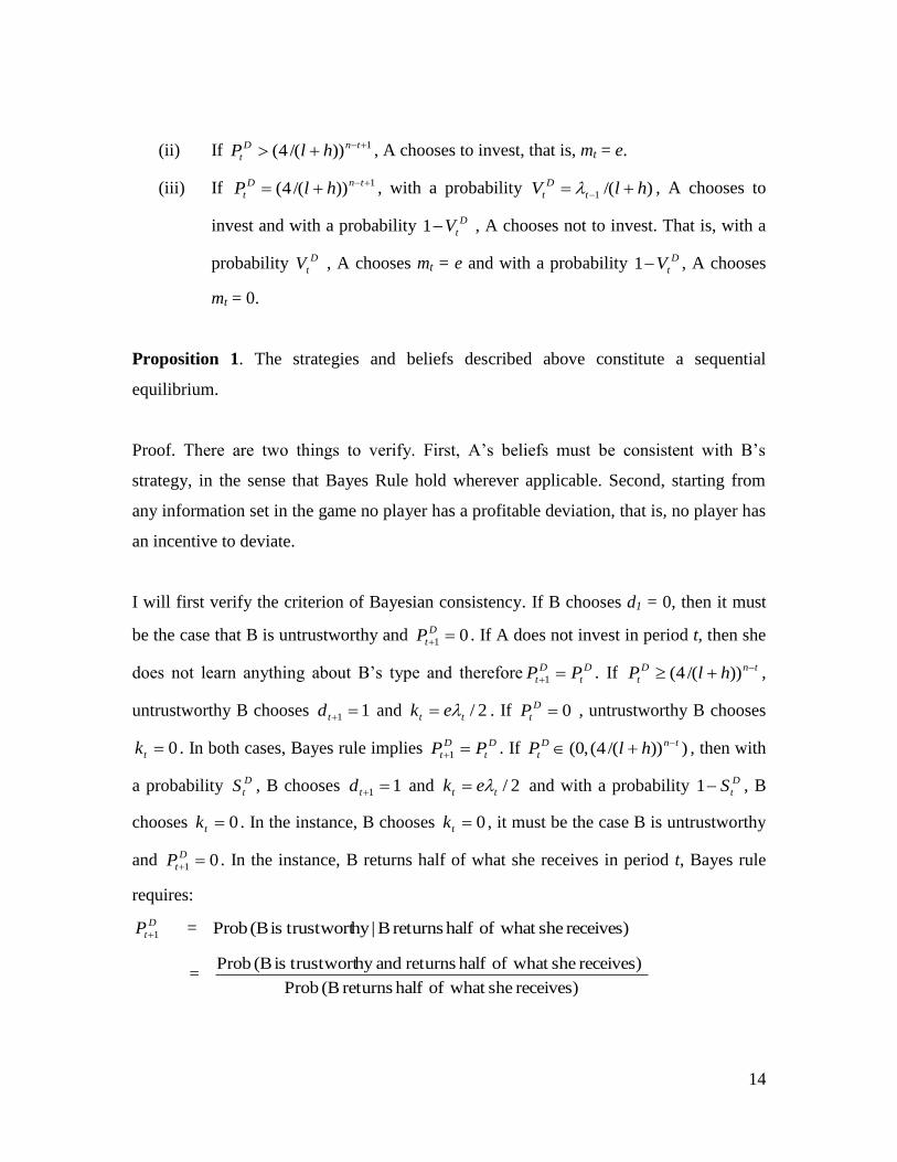
Proposition 1. The strategies and beliefs described above constitute a sequential

equilibrium.

Proof. There are two things to verify. First, A‟s beliefs must be consistent with B‟s

strategy, in the sense that Bayes Rule hold wherever applicable. Second, starting from

any information set in the game no player has a profitable deviation, that is, no player has

an incentive to deviate.

I will first verify the criterion of Bayesian consistency. If B chooses d1 = 0, then it must

be the case that B is untrustworthy and 01

D

tP . If A does not invest in period t, then she

does not learn anything about B‟s type and therefore D

t

D

t PP 1 . If tnD

t hlP ))/(4( ,

untrustworthy B chooses 11 td and 2/tt ek . If 0D

tP , untrustworthy B chooses

0tk . In both cases, Bayes rule implies D

t

D

t PP 1 . If )))/(4(,0( tnD

t hlP , then with

a probability D

tS , B chooses 11 td and 2/tt ek and with a probability D

tS1 , B

chooses 0tk . In the instance, B chooses 0tk , it must be the case B is untrustworthy

and 01

D

tP . In the instance, B returns half of what she receives in period t, Bayes rule

requires:

D

tP 1 = receives) she what of half returns B |hy trustwortis (B Prob

= receives) she what of half returns (B Prob

receives) she what of half returns andhy trustwortis (B Prob

15

=

thy)untrustwor is (B Prob thy)untrustwor is B | half returns (B Prob

+ hy) trustwortis (B Prob hy) trustwortis B | half returns (B Prob

hy) trustwortis (B Prob hy) trustwortis B | half returns (B Prob

= )1(.1

.1D

t

D

t

D

t

D

t

PSP

P

=

tn

hl

4

This satisfies the criterion of Bayesian consistency.

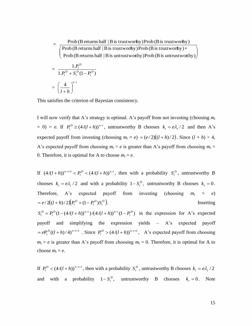
I will now verify that A‟s strategy is optimal. A‟s payoff from not investing (choosing mt

= 0) = e. If tnD

t hlP ))/(4( , untrustworthy B chooses 2/tt ek and then A‟s

expected payoff from investing (choosing mt = e) 2/)()2/( hle . Since (l + h) > 4,

A‟s expected payoff from choosing mt = e is greater than A‟s payoff from choosing mt =

0. Therefore, it is optimal for A to choose mt = e.

If tnD

t

tn hlPhl ))/(4())/(4( 1 , then with a probability D

tS , untrustworthy B

chooses 2/tt ek and with a probability ,1 D

tS untrustworthy B chooses 0tk .

Therefore, A‟s expected payoff from investing (choosing mt = e)

D

t

D

t

D

t SPPhle )1(2/)(2/ . Inserting

)1())/(4/()))/(4(1( D

t

tntnD

t

D

t PhlhlPS in the expression for A‟s expected

payoff and simplifying the expression yields – A‟s expected payoff

1)4/)(( tnD

t hleP . Since 1))/(4( tnD

t hlP , A‟s expected payoff from choosing

mt = e is greater than A‟s payoff from choosing mt = 0. Therefore, it is optimal for A to

choose mt = e.

If 1))/(4( tnD

t hlP , then with a probability D

tS , untrustworthy B chooses 2/tt ek

and with a probability ,1 D

tS untrustworthy B chooses 0tk . Note

16

.))/(4())/(4( 1 tntnD

t hlhlP Now, A‟s expected payoff from investing (choosing

mt = e) D

t

D

t

D

t SPPhle )1(2/)(2/ . Once again, inserting

)1())/(4/()))/(4(1( D

t

tntnD

t

D

t PhlhlPS in the expression for A‟s expected

payoff and simplifying the expression yields – A‟s expected payoff

1)4/)(( tnD

t hleP . However, since 1))/(4( tnD

t hlP , A‟s expected payoff from

choosing mt = e is less than A‟s payoff from choosing mt = 0. Therefore, it is optimal for

A to choose mt = 0.

If 1))/(4( tnD

t hlP then A‟s expected payoff from investing (choosing mt = e)

D

t

D

t

D

t SPPhle )1(2/)(2/ . Now .))/(4())/(4( 1 tntnD

t hlhlP Recall that

if tnD

t hlP ))/(4( , then with a probability D

tS , untrustworthy B chooses 2/tt ek

and with a probability ,1 D

tS untrustworthy B chooses 0tk . Once again, inserting

)1())/(4/()))/(4(1( D

t

tntnD

t

D

t PhlhlPS in the expression for A‟s expected

payoff and simplifying the expression yields – A‟s expected payoff

1)4/)(( tnD

t hleP . However, since 1))/(4( tnD

t hlP , A‟s expected payoff from

choosing mt = e is equal to A‟s payoff from choosing mt = 0. At this point, A is

indifferent between choosing mt = e and choosing mt = 0. Therefore, with a probability

D

tV , A chooses mt = e and with a probability D

tV1 , A chooses mt = 0. The choice of the

probability D

tV is such that it makes B indifferent between choosing 2/11 tt ek and

choosing 01 tk . To verify B‟s indifference at this point, note that B‟s payoff from

choosing 01 tk is 1te and B‟s expected payoff from choosing 2/11 tt ek is

2/)(2/1 hleVe D

tt . Since )/(1 hlV t

D

t , B‟s expected payoff from choosing

01 tk equals B‟s payoff from choosing 2/11 tt ek .

17

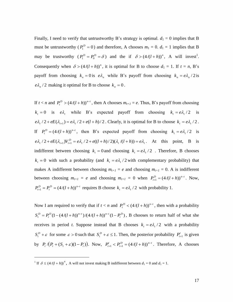
Finally, I need to verify that untrustworthy B‟s strategy is optimal. d1 = 0 implies that B

must be untrustworthy ( 01 DP ) and therefore, A chooses m1 = 0. d1 = 1 implies that B

may be trustworthy ( DD PP 01 ) and the if nhl ))/(4( , A will invest1.

Consequently when nhl ))/(4( , it is optimal for B to choose d1 = 1. If t = n, B‟s

payoff from choosing 0nk is ne while B‟s payoff from choosing 2/nn ek is

2/ne making it optimal for B to choose 0nk .

If t < n and tnD

t hlP ))/(4( , then A chooses mt+1 = e. Thus, B‟s payoff from choosing

0tk

is te

while B‟s expected payoff from choosing 2/tt ek

is

2/)(2/)(2/ 1 hleeeEe ttt . Clearly, it is optimal for B to choose 2/tt ek .

If tnD

t hlP ))/(4( , then B‟s expected payoff from choosing 2/tt ek

is

ttt

D

ttt ehlhleeVeEe ))/()(2/)((2/)(2/ 11 . At this point, B is

indifferent between choosing 0tk and choosing 2/tt ek . Therefore, B chooses

0tk with such a probability (and 2/tt ek with complementary probability) that

makes A indifferent between choosing mt+1 = e and choosing mt+1 = 0. A is indifferent

between choosing mt+1 = e and choosing mt+1 = 0 when tnD

t hlP

))/(4(1 . Now,

tnD

t

D

t hlPP

))/(4(1 requires B choose 2/tt ek with probability 1.

Now I am required to verify that if t < n and tnD

t hlP ))/(4( , then with a probability

)1())/(4/()))/(4(1( D

t

tntnD

t

D

t PhlhlPS , B chooses to return half of what she

receives in period t. Suppose instead that B chooses 2/tt ek with a probability

D

tS for some 0 such that 1D

tS . Then, the posterior probability 1

tP is given

by )1)((/ tttt PSPP . Now, tnD

tt hlPP

))/(4(11 . Therefore, A chooses

1 If ,))/(4(

nhl

A will not invest making B indifferent between d1 = 0 and d1 = 1.

18

mt+1 = 0. This implies the sum of B‟s expected payoff in periods t and (t+1) =

))(2/()1( tttt SeSe . In contrast, if B chooses 2/ttk with a probability

D

tS then her expected payoff = tttttttt eeVeSSeE )2/()1( 11 . Since B‟s

expected payoff from choosing 2/tt ek with a probability D

tS is higher than her

expected payoff from choosing 2/tt ek with a probability D

tS , she will not

choose 2/tt ek with a probability D

tS . Similarly, it can be shown that B will not

choose 2/tt ek with a probability D

tS for some 0 such that 0D

tS . The

only case remaining to be ruled out is one where B choose 2/tt ek with a probability

D

tS for some 0 such that 0D

tS . That is, the case where B never chooses

2/tt ek . In this case, the posterior probability 11 tP . That is, given a return of

2/tt ek , A believes with probability 1 that B is trustworthy. This strategy can never

constitute an equilibrium because a profitable deviation for an untrustworthy B is to

mimic to be the trustworthy type and choose 2/tt ek and then because 11

tP , A

will chose mt+1 = e.

This completes the proof that the set of beliefs and strategies described earlier constitutes

a sequential equilibrium.

Reputation Threshold. D

tP 1 must be at least 1))/(4( tnhl

for A to invest with some

probability. This threshold 1))/(4( tnhl may be thought of as B‟s reputation. B starts

mixed strategy play in some period t to ensure that A‟s updated (period t+1) belief about

B‟s type is exactly on the threshold. This threshold increases in t. That is, B‟s reputation

over time must be progressively higher for A to invest. For example, if n = 10, l = 1 and h

= 5, then this reputation threshold may be graphed as in Figure 2A.

19

Figure 2A – Reputation Threshold at which A invests with some probability when n = 10,

l = 1 and h = 5

Full Disclosure Strategy. What happens if untrustworthy B follows a strategy of

choosing 1td and 2/tt ek ? That is, untrustworthy B chooses to mimic to be the

trustworthy type with probability 1. This strategy will be a part of the equilibrium

described earlier if )/(40 hlPD . However, when )/(40 hlPD , then by Bayesian

updating DD

t

D

t PPP 01 ...... . At some t = i, 1)/(4

inD

i hlP and therefore, A will

not invest in any period it . In contrast, if B follows the strategy outlined in the

equilibrium described earlier, A will invest with some positive probability in period it .

In other words, full disclosure does not constitute equilibrium and will result in lower

investment. In equilibrium, B will mimic to be the trustworthy type but will do so

selectively instead of indiscriminately in order to ensure the credibility associated with

her choice in the instances where she actually chooses to mimic (except when

)/(40 hlPD ).

0

0.1

0.2

0.3

0.4

0.5

0.6

0.7

1 2 3 4 5 6 7 8 9 10

Period

A's Threshold

A's Threshold

20

For example, if n = 10, l = 1, h = 5 and 4.00 DP , then the reputation threshold is given

by the blue dotted line in Figure 2B. The way A‟s belief about B‟s type evolves in

equilibrium and under the full disclosure strategy respectively is shown by the red dotted

line and the green dotted line in Figure 2B. Note that under full disclosure strategy, A‟s

belief falls below the reputation threshold in period 9 but remains on the threshold under

equilibrium. Consequently, under full disclosure, A does not invest in periods 9 and 10

but in equilibrium, A may invest in both periods.

Figure 2B – Reputation Threshold at which A invests with some probability and A’s

beliefs about B’s type when n = 10, l = 1 , h = 5 and 4.00 DP

4. No Disclosure Regime

Now consider a world without disclosure. As before, there are two players, A (sender /

investor) and B (receiver / manager). Nature moves first and selects B‟s type to be either

trustworthy or untrustworthy. I will define momentarily what I mean by each type in this

regime. B knows her type but A does not. The game then proceeds through n periods in

each of which the A and B make a sequence of choices. In what follows, the subscript t (t

0

0.1

0.2

0.3

0.4

0.5

0.6

0.7

1 2 3 4 5 6 7 8 9 10

Period

A's Threshold and Beliefs

A's Threshold

A's Beliefs in Disclosure

Regime

A's beliefs if B plays

'Full Disclosure' strategy

21

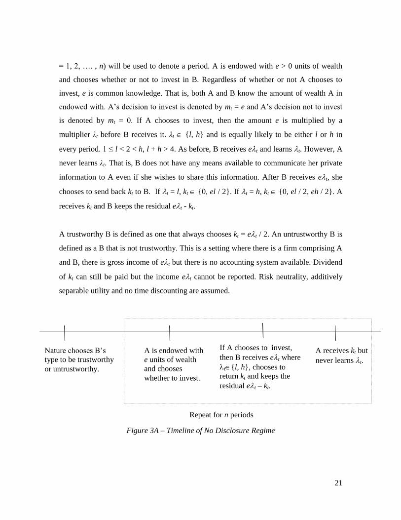
= 1, 2, …. , n) will be used to denote a period. A is endowed with e > 0 units of wealth

and chooses whether or not to invest in B. Regardless of whether or not A chooses to

invest, e is common knowledge. That is, both A and B know the amount of wealth A in

endowed with. A‟s decision to invest is denoted by mt = e and A‟s decision not to invest

is denoted by mt = 0. If A chooses to invest, then the amount e is multiplied by a

multiplier λt before B receives it. λt {l, h} and is equally likely to be either l or h in

every period. 1 ≤ l < 2 < h, l + h > 4. As before, B receives et and learns t. However, A

never learns λt. That is, B does not have any means available to communicate her private

information to A even if she wishes to share this information. After B receives et, she

chooses to send back kt to B. If t = l, kt {0, el / 2}. If t = h, kt {0, el / 2, eh / 2}. A

receives kt and B keeps the residual et - kt.

A trustworthy B is defined as one that always chooses kt = et / 2. An untrustworthy B is

defined as a B that is not trustworthy. This is a setting where there is a firm comprising A

and B, there is gross income of et but there is no accounting system available. Dividend

of kt can still be paid but the income et cannot be reported. Risk neutrality, additively

separable utility and no time discounting are assumed.

Figure 3A – Timeline of No Disclosure Regime

Nature chooses B‟s

type to be trustworthy

or untrustworthy.

A is endowed with

e units of wealth

and chooses

whether to invest.

If A chooses to invest,

then B receives et where

t{l, h}, chooses to

return kt and keeps the

residual et – kt.

A receives kt but

never learns t.

Repeat for n periods

22

Figure 3B – Extensive Form Representation of the Stage Game in No Disclosure Regime

A sequential equilibrium of this game is defined as follows. An equilibrium comprises a

strategy for each player and for each period t a function ND

tP that takes the history of

moves up to period t into numbers in [0 , 1] such that :

(i) Starting from any point in the game where it is B‟s move, B‟s strategy is a

best response to A‟s strategy.

(ii) Starting from any point in the game where it is A‟s move, A‟s strategy is a

best response to B‟s strategy given that A believes B is trustworthy with

probability )( t

ND

t hP .

(iii) The game begins with .1 NDP

(iv) Each ND

tP is computed from ND

tP 1 and B‟s strategy, using Bayes‟ rule

whenever possible.

e , 0

mt = 0 mt = e

A

B

t = h,

kt = l/2

t = l,

kt =0

t = h,

kt = 0

t = l,

kt = l/2

t = h,

kt = h/2 0, el

el/2, el/2

0, eh

el/2, eh-el/2 eh/2, eh/2

23

I will first define the function ND

tP as:

(i) Set .1 NDP

(ii) For t > 1, if A chooses mt-1 = 0, then ND

t

ND

t PP 1 .

(iii) For t > 1, if A chooses mt-1 = e and B chooses kt-1 > 0 and 01

ND

tP , then

.))12(2/(,))/(4(max 111 tttnND

t hlP .

(iv) For t > 1, if A chooses mt-1 = e but B chooses 01 tk , then 0ND

tP .

(v) If 01

ND

tP , then 0ND

tP .

Now, I will describe the strategies of A and untrustworthy B in terms of ND

tP . Note that

by definition, a trustworthy B always to return half of what she receives. An

untrustworthy B‟s strategy depends on t and ND

tP . The strategy may be outlined as:

(i) If t = n, B chooses 0nk .

(ii) If t < n and tntnND

t hlhlP ))/(4(1/))/(4.(2 , B chooses 2/elkt .

(iii) If t < n and tntnND

t hlhlP ))/(4(1/))/(4.(2 and lt , B chooses

2/elkt with some probability ND

tS3 )10( 3 ND

tS and chooses 0tk with

probability ND

tS31 .

(iv) If t < n and tntnND

t hlhlP ))/(4(1/))/(4.(2 and ht , B chooses

2/ehkt with some probability ND

tS1 )10( 1 ND

tS , chooses 2/elkt with

some probability ND

tS2 )10,10( 212 ND

t

ND

t

ND

t SSS and chooses 0tk

with probability ND

t

ND

t SS 211

such that

)1())/(4/()))/(4(1(321

ND

t

tntnND

t

ND

t

ND

t

ND

t PhlhlPSSS .

A‟s strategy may be outlined as:

(i) If 1))/(4( tnND

t hlP , A chooses mt = 0.

24

(ii) If 1))/(4( tnND

t hlP , A chooses mt = e.

(iii) If 1))/(4( tnND

t hlP and 2/1 ehkt , with a probability )/(1 hlhV ND

t ,

A chooses to invest and with a probability ND

tV11 , A chooses not to invest.

That is, with a probability ND

tV1 , A chooses mt = e and with a probability

ND

tV11 , A chooses mt = 0.

(iv) If 1))/(4( tnND

t hlP and 2/1 elkt , with a probability )/(2 hllV ND

t ,

A chooses to invest and with a probability ND

tV21 , A chooses not to invest.

That is, with a probability ND

tV2 , A chooses mt = e and with a probability

ND

tV21 , A chooses mt = 0.

Proposition 2. The strategies and beliefs described above constitute a sequential

equilibrium.

Proof. There are two things to verify. First, A‟s beliefs must be consistent with B‟s

strategy, in the sense that Bayes Rule hold wherever applicable. Second, starting from

any information set in the game no player has a profitable deviation, that is, no player has

an incentive to deviate.

I will first verify the criterion of Bayesian consistency. If A does not invest in period t,

then she does not learn anything about B‟s type and therefore ND

t

ND

t PP 1 . If 0ND

tP ,

untrustworthy B chooses 0tk and Bayes rule implies ND

t

ND

t PP 1 .

If tntnND

t hlhlP ))/(4(1/))/(4.(2 , untrustworthy B chooses 2/elkt and

Bayes Rule requires:

ND

tP 1 = )2/ chooses B |hy trustwortis (B Prob elkt

25

= )2/ chooses (B Prob

)2/ chooses andhy trustwortis (B Prob

elk

elk

t

t

=

thy)untrustwor is (B Prob thy)untrustwor is B | 2/ chooses (B Prob

+ hy) trustwortis (B Prob hy) trustwortis B | 2/ chooses (B Prob

hy) trustwortis (B Prob hy) trustwortis B | 2/ chooses (B Prob

elk

elk

elk

t

t

t

= )1(.2/1

.2/1D

t

ND

t

ND

t

PP

P

= ND

t

ND

t

P

P

2

=

)12(2 11 tt, since .1 NDP

Now, if tntnND

t hlhlP ))/(4(1/))/(4.(2 and 2/elkt , it could be lt and

B chose 2/elkt with probability ND

tS3 )10( 3 ND

tS or it could be ht and B chose

2/ehkt with probability ND

tS2 )10( 2 ND

tS . Recall that

)1())/(4/()))/(4(1(32

ND

t

tntnND

t

ND

t

ND

t PhlhlPSS . By Bayes Rule:

ND

tP 1 = )2/ chooses B |hy trustwortis (B Prob elkt

= )2/ chooses (B Prob

)2/ chooses andhy trustwortis (B Prob

elk

elk

t

t

=

) receives andthy untrustwor is (B Prob

thy)untrustwor is B | 2/ chooses (B Prob ) receives and

thy untrustwor is (B Prob thy)untrustwor is B | 2/ chooses (B Prob

+ hy) trustwortis (B Prob hy) trustwortis B | 2/ chooses (B Prob

hy) trustwortis (B Prob hy) trustwortis B | 2/ chooses (B Prob

eh

elkel

elk

elk

elk

t

t

t

t

= ND

t

ND

t

ND

t

ND

t

ND

t

ND

t

SPSPP

P

23 )1.(2/1)1.(2/1.2/1

.2/1

= ))(1( 23

ND

t

ND

t

ND

t

ND

t

ND

t

SSPP

P

26

=

14

tn

hl

Finally, if tntnND

t hlhlP ))/(4(1/))/(4.(2 and ht , B chooses 2/ehkt with

probability )1())/(4/()))/(4(1(1

ND

t

tntnND

t

ND

t PhlhlPS . By Bayes Rule:

ND

tP 1 = )2/ chooses B |hy trustwortis (B Prob ehkt

= )2/ chooses (B Prob

)2/ chooses andhy trustwortis (B Prob

ehk

ehk

t

t

=

thy)untrustwor is (B Prob thy)untrustwor is B | 2/ chooses (B Prob

+ hy) trustwortis (B Prob hy) trustwortis B | 2/ chooses (B Prob

hy) trustwortis (B Prob hy) trustwortis B | 2/ chooses (B Prob

ehk

ehk

ehk

t

t

t

= ND

t

ND

t

ND

t

ND

t

SPP

P

1)1.(2/1.2/1

.2/1

=

14

tn

hl

This satisfies the criterion of Bayesian consistency.

I will now verify that A‟s strategy is optimal. A‟s payoff from not investing (choosing mt

= 0) = e. If tntnND

t hlhlP ))/(4(1/))/(4.(2 , B chooses 2/elkt . A‟s

expected payoff from investing (choosing mt = e) = )2/)(1(4/)( lPehleP ND

t

ND

t is

greater than A‟s payoff from not investing (choosing mt = 0) = e if

elPehleP ND

t

ND

t )2/)(1(4/)( . Simplifying yields A‟s expected payoff from

choosing mt = e is higher if )/()2.(2 lhlPND

t . Now by definition of ND

tP , it must be

that ))12(2/( 11 ttND

tP and ).)12(2/(1

ttND

tP Algebraic simplification

yields ).2/(1

ND

t

ND

t

ND

t PPP Also, tnttND

t hlP

))/(4())12(2/(1

by

definition of .ND

tP

That is, .))/(4()2/(1

tnND

t

ND

t

ND

t hlPPP

Simplifying

27

tntntnND

t hlP 4)(/4.2 and I will have proved A‟s payoff from choosing mt = e is

higher if I can show .4)(/4.2)/()2.(2 tntntn hllhl Re-arranging this

inequality is equivalent to .4.).(4.2).(2 tntntntn hhllhl I will prove this by

induction. Denote .4.).(4.2).(2 tntntntn hhllhl by *. At t = n – 1, LHS of (*)

= 2.(l + h + 4) and RHS of (*) = l2 + lh + 4h. This LHS < RHS since (l + h) > 4.

Suppose LHS < RHS for some t = k+1. That is,

.4.).(4.2).(2 1111 knknknkn hhllhl

Multiplying both sides by (l+h) yields –

)(4.).()(4.2).(2 11 hlhhllhlhl knknknkn ……….. (**)

At t =k, (*) becomes .4.).(4.2).(2 knknknkn hhllhl ……….. (***)

LHS of (***) = knknhl 4.2).(2

)(4.2).(2 1 hlhl knkn (since 4 < l+h)

)(4.).( 1 hlhhll knkn (from **)

knkn hhll 4.).( (since 4 < l+h) = RHS of (***).

This completes the proof by induction. Note that

tntnND

t hlhlP ))/(4(1/))/(4.(2

implies 1))/(4( tnND

t hlP since it can be

shown that .))/(4(1/))/(4.(2))/(4( 1 tntntn hlhlhl .

If tntnND

t hlhlP ))/(4(1/))/(4.(2 and lt , B chooses 2/elkt with

probability ND

tS3 and chooses 0tk with probability ND

tS31 . If

tntnND

t hlhlP ))/(4(1/))/(4.(2 and ht , B chooses 2/ehkt with

probability ND

tS1 , chooses 2/elkt with probability ND

tS2 and chooses 0tk with

probability ND

t

ND

t SS 211 . This implies A‟s expected payoff from investing (choosing mt

= e) = .)4/)(1())(4/)(1(4/)( 132

ND

t

ND

t

ND

t

ND

t

ND

t

ND

t ShPeSSlPehleP Inserting

the expressions for ND

tS1 and )( 32

ND

t

ND

t SS and simplifying yields A‟s expected payoff

28

from investing = .4/)(1

tnND

t hleP Now ehlePtnND

t 1

4/)( if

.))/(4( 1 tnND

t hlP

That is, when tntnND

t hlhlP ))/(4(1/))/(4.(2 , it is

optimal for A to invest if 1))/(4( tnND

t hlP and not to invest if .))/(4( 1 tnND

t hlP

At ,))/(4( 1 tnND

t hlP

A‟s payoff from investing equals A‟s payoff from not

investing. That is, A is indifferent between choosing mt = e and choosing mt = 0.

Therefore, A chooses to invest with a probability that makes B indifferent between the

options available to her. That is when, 2/1 elkt , with a probability )/(2 hllV ND

t , A

chooses to invest and with a probability ND

tV21 , A chooses not to invest. To verify B‟s

indifference at this point, note that if ,1 lt B‟s payoff from choosing 01 tk is el

and B‟s expected payoff from choosing 2/1 elkt is 2/)(2/ 2 hleVel ND

t . Since

)/(2 hllV ND

t , B‟s expected payoff from choosing 01 tk equals B‟s payoff from

choosing 2/1 elkt . If ,1 ht B‟s payoff from choosing 01 tk is eh and B‟s

expected payoff from choosing 2/1 elkt is 2/)(2/ 2 hleVeleh ND

t . Since

)/(2 hllV ND

t , B‟s expected payoff from choosing 01 tk equals B‟s payoff from

choosing 2/1 elkt . Now when, 2/1 ehkt , with a probability )/(1 hlhV ND

t , A

chooses to invest and with a probability ND

tV11 , A chooses not to invest. To verify B‟s

indifference at this point, note that B‟s payoff from choosing 01 tk is eh and B‟s

expected payoff from choosing 2/1 ehkt is 2/)(2/ 2 hleVeh ND

t . Since

)/(1 hlhV ND

t , B‟s expected payoff from choosing 01 tk equals B‟s payoff from

choosing 2/1 ehkt .

29

Finally, I need to verify that untrustworthy B‟s strategy is optimal. If t = n, B‟s payoff

from choosing 0nk is ne while B‟s payoff from not choosing 0nk is strictly lower

making it optimal for B to choose 0nk .

If t < n and tntnND

t hlhlP ))/(4(1/))/(4.(2 , then A chooses mt+1 = e since

tntnND

t hlhlP ))/(4(1/))/(4.(2 implies tnND

t hlP

))/(4(1 . (It can be shown

that tntntn hlhlhl ))/(4())/(4(1/))/(4.(2 ). Thus, B‟s payoff from choosing

0tk

is te

while B‟s expected payoff from choosing 2/elkt is

2/)(2/)(2/ 1 hleeleeEele ttt . Clearly, it is optimal for B to choose

2/elkt .

If t < n and tntnND

t hlhlP ))/(4(1/))/(4.(2 , then by definition of ND

tP , it must

be that tnND

t hlP

))/(4(1 . If lt

and 2/elkt , then with a probability

)/(2 hllV ND

t , A chooses mt+1 = e and with a probability ND

tV21 , A chooses mt+1 = 0.

Thus, while B‟s payoff from choosing 0tk is el , B‟s expected payoff from choosing

2/elkt is )/()2/)((2/)(2/ 21 hllhleelVeEel ND

tt . At this point, B is

indifferent between choosing 0tk and choosing 2/elkt . Therefore, B chooses

2/elkt with probability ND

tS3 (and 0tk with complementary probability) that makes

A indifferent between choosing mt+1 = e and choosing mt+1 = 0. If t < n and

tntnND

t hlhlP ))/(4(1/))/(4.(2 , ht

and 2/elkt , then also with a

probability )/(2 hllV ND

t , A chooses mt+1 = e and with a probability ND

tV21 , A

chooses mt+1 = 0. Again, while B‟s payoff from choosing 0tk is eh , B‟s expected

payoff from choosing 2/elkt is ND

tt VeEeleh 21)(2/

)/()2/)((2/ hllhleeleh . Therefore at this point too, B is indifferent between

30

choosing 0tk and choosing 2/elkt . B chooses 2/elkt

with probability ND

tS2 (

2/ehkt with probability ND

tS1 and 0tk

with probability ND

t

ND

t SS 211 ) that makes

A indifferent between choosing mt+1 = e and choosing mt+1 = 0. A is indifferent between

choosing mt+1 = e and choosing mt+1 = 0 when tnD

t hlP

))/(4(1 . By Bayes Rule,

))(1(/ 231

ND

t

ND

t

ND

t

ND

t

ND

t

ND

t SSPPPP . Inserting ND

t

ND

t SS 32

)1())/(4/()))/(4(1( ND

t

tntnND

t PhlhlP and simplifying, we get

tnD

t hlP

))/(4(1 .

If t < n and tntnND

t hlhlP ))/(4(1/))/(4.(2 , ht and 2/ehkt , then with a

probability )/(1 hlhV ND

t , A chooses mt = e and with a probability ND

tV11 , A chooses

mt = 0. B‟s payoff from choosing 0tk is eh while B‟s expected payoff from choosing

2/ehkt is ND

tt VeEeh 11)(2/ )/()2/)((2/ hlhhleeh . This makes B

indifferent between choosing 0tk and choosing 2/ehkt . B chooses 2/ehkt

with

probability ND

tS1 ( 2/elkt with probability ND

tS2 and 0tk

with probability

ND

t

ND

t SS 211 ) that makes A indifferent between choosing mt+1 = e and choosing mt+1 =

0. A is indifferent between choosing mt+1 = e and choosing mt+1 = 0 when

tnD

t hlP

))/(4(1 . By Bayes Rule, ND

t

ND

t

ND

t

ND

t

ND

t SPPPP 11 )1(/ . Inserting ND

tS1

)1())/(4/()))/(4(1( ND

t

tntnND

t PhlhlP and simplifying, we get

tnD

t hlP

))/(4(1 .

This completes the proof that the set of beliefs and strategies described earlier constitutes

a sequential equilibrium.

The reputation threshold in the no disclosure regime turns out to the same as the

reputation threshold in the disclosure regime. That is, D

tP 1 and ND

tP 1 in the disclosure and

31

no disclosure regimes respectively must be at least 1))/(4( tnhl for A to invest with

some positive probability.

5. Investment, Return and Disclosure

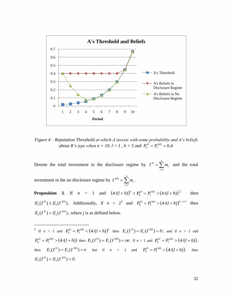
Consider n = 10, l = 1, h = 5 and 4.010 NDD PP . Then, the way A‟s belief about B‟s

type evolves in the disclosure and no disclosure regimes respectively is shown by the red

dotted line and the green dotted line in Figure 4. Note that when A‟s belief is above the

reputation threshold, A plays a pure strategy of always investing. When A‟s belief is on

the threshold, A switches to a mixed strategy play where the probability with which she

invests is given by the equilibrium described earlier. B switches to mixed strategy play to

prevent A‟s beliefs from falling below the threshold. In this example, even though the

game in both regimes begins with identical initial probability of 0.4, the disclosure

regime provides for more time of pure strategy play as compared to the no disclosure

regime. In this sense, the disclosure regime provides for additional reputation building

opportunities. Since probability of investment in a period of pure strategy play is higher

than probability of investment in a period of mixed strategy play, therefore more time of

pure strategy play in a disclosure regime should translate into higher investment in

disclosure regime.

32

Figure 4 – Reputation Threshold at which A invests with some probability and A’s beliefs

about B’s type when n = 10, l = 1 , h = 5 and 4.010 NDD PP

Denote the total investment in the disclosure regime by

n

t

t

D mI1

and the total

investment in the no disclosure regime by

n

t

t

ND mI1

.

Proposition 3. If n > 1 and )/(4)/(4 10 hlPPhl NDDn

2 then

)()( 11

NDD IEIE . Additionally, if n > 23 and 1

10 )/(4

jnNDD hlPP

then

)()( 11

NDD IEIE , where j is as defined below.

2 If n > 1 and nNDD hlPP )/(410

then 0)()( 11 NDD IEIE ; and if n > 1 and

)/(410 hlPP NDD then neIEIE NDD )()( 11 . If n = 1 and )/(410 hlPP NDD ,

then eIEIE NDD )()( 11 but if n = 1 and )/(410 hlPP NDD , then

0)()( 11 NDD IEIE .

0

0.1

0.2

0.3

0.4

0.5

0.6

0.7

1 2 3 4 5 6 7 8 9 10

Period

A's Threshold and Beliefs

A's Threshold

A's Beliefs in

Disclosure Regime

A's Beliefs in No

Disclosure Regime

33

Proof. Let .10 NDD PP

By definition, ,))/(4(max 1 tnD

t hlP and

.))12(2/(,))/(4(max 111 tttnND

t hlP At some t = k, .))/(4( 1 knD

k hlP

For t < k, D

tP and for t > k, .))/(4( 1 tnD

t hlP Also, at some t = j,

.))/(4( 1 jnND

j hlP

For t < j, ))12(2/( 11 ttND

tP and for t > j,

.))/(4( 1 tnND

t hlP At t < k, A invests with probability 1 in the disclosure regime and

similarly at t < j, A invests with probability 1 in the no disclosure regime. However, at

kt and jt in the disclosure and no disclosure regimes respectively, A invests with a

probability less than 1. Now, D

tP

is constant over time while

))12(2/( 11 ttND

tP is a decreasing function. Therefore, jk and this implies

that )()( 11

NDD IEIE . That is, there is at least as much period of time in the disclosure

regime where A invests with probability 1 as there is in the no disclosure regime and

therefore, expected investment in the disclosure regime will be at least as high as in the

no disclosure regime.

If 1

10 )/(4

jnNDD hlPP , then ND

j

jnknD

k PhlhlP 11 )/(4))/(4( .

This implies k > j and therefore, )()( 11

NDD IEIE . That is, there is greater period of

time in the disclosure regime where A invests with probability 1 than there is in the no

disclosure regime and therefore, expected investment in the disclosure regime will be

higher than in the no disclosure regime.

3 If n = 2 and )/(4)/(4 10 hlPPhl NDDn

, then k = j = 2 and )()( 11

NDD IEIE .

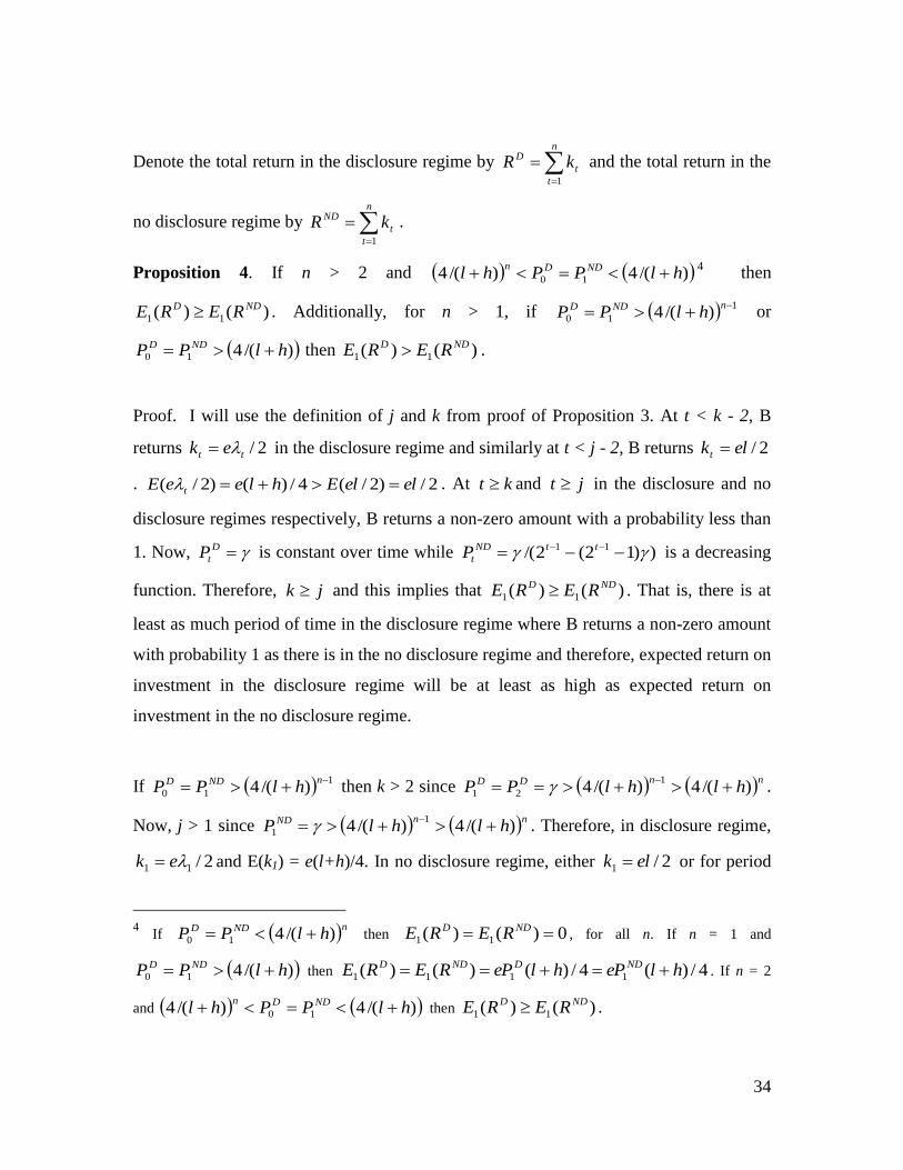
34

Denote the total return in the disclosure regime by

n

t

t

D kR1

and the total return in the

no disclosure regime by

n

t

t

ND kR1

.

Proposition 4. If n > 2 and )/(4)/(4 10 hlPPhl NDDn

4 then

)()( 11

NDD RERE . Additionally, for n > 1, if 1

10 )/(4

nNDD hlPP

or

)/(410 hlPP NDD then )()( 11

NDD RERE .

Proof. I will use the definition of j and k from proof of Proposition 3. At t < k - 2, B

returns 2/tt ek in the disclosure regime and similarly at t < j - 2, B returns 2/elkt

. 2/)2/(4/)()2/( elelEhleeE t . At kt and jt in the disclosure and no

disclosure regimes respectively, B returns a non-zero amount with a probability less than

1. Now, D

tP is constant over time while ))12(2/( 11 ttND

tP is a decreasing

function. Therefore, jk and this implies that )()( 11

NDD RERE . That is, there is at

least as much period of time in the disclosure regime where B returns a non-zero amount

with probability 1 as there is in the no disclosure regime and therefore, expected return on

investment in the disclosure regime will be at least as high as expected return on

investment in the no disclosure regime.

If 1

10 )/(4

nNDD hlPP then k > 2 since nnDD hlhlPP )/(4)/(4

1

21

.

Now, j > 1 since nnND hlhlP )/(4)/(41

1

. Therefore, in disclosure regime,

2/11 ek and E(k1) = e(l+h)/4. In no disclosure regime, either 2/1 elk or for period

4 If nNDD hlPP )/(410

then 0)()( 11 NDD RERE , for all n. If n = 1 and

)/(410 hlPP NDD then 4/)(4/)()()( 1111 hlePhlePRERE NDDNDD . If n = 2

and )/(4)/(4 10 hlPPhl NDDn

then )()( 11

NDD RERE .

35

1, B returns a non-zero amount with a probability less than 1. But in either of the two

cases in no disclosure regime, E(k1) < e(l+h)/4. This implies )()( 11

NDD RERE .

Similarly, if )/(410 hlPP NDD then in disclosure regime, E(k1) = e(l+h)/4. But in

no disclosure regime, either 2/1 elk or for period 1, B returns a non-zero amount with

a probability less than 1 which in turn implies E(k1) < e(l+h)/4. That is,

)()( 11

NDD RERE . In other words, expected return on investment in the disclosure

regime will be higher than expected return on investment in the no disclosure regime.

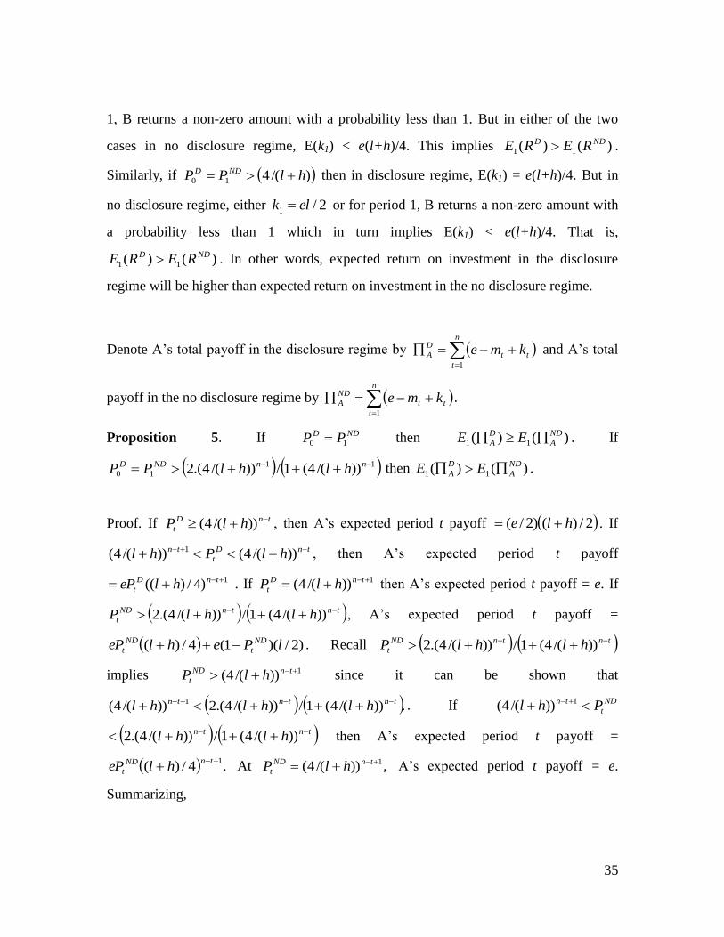
Denote A‟s total payoff in the disclosure regime by

n

t

tt

D

A kme1

and A‟s total

payoff in the no disclosure regime by

n

t

tt

ND

A kme1

.

Proposition 5. If NDD PP 10 then )()( 11

ND

A

D

A EE . If

11

10 ))/(4(1/))/(4.(2 nnNDD hlhlPP then )()( 11

ND

A

D

A EE .

Proof. If tnD

t hlP ))/(4( , then A‟s expected period t payoff 2/)()2/( hle . If

tnD

t

tn hlPhl ))/(4())/(4( 1 , then A‟s expected period t payoff

1)4/)(( tnD

t hleP . If 1))/(4( tnD

t hlP then A‟s expected period t payoff = e. If

tntnND

t hlhlP ))/(4(1/))/(4.(2 , A‟s expected period t payoff =

)2/)(1(4/)( lPehleP ND

t

ND

t . Recall tntnND

t hlhlP ))/(4(1/))/(4.(2

implies 1))/(4( tnND

t hlP

since it can be shown that

.))/(4(1/))/(4.(2))/(4( 1 tntntn hlhlhl . If ND

t

tn Phl 1))/(4(

tntn hlhl ))/(4(1/))/(4.(2

then A‟s expected period t payoff =

.4/)(1

tnND

t hleP At ,))/(4( 1 tnND

t hlP

A‟s expected period t payoff = e.

Summarizing,

36

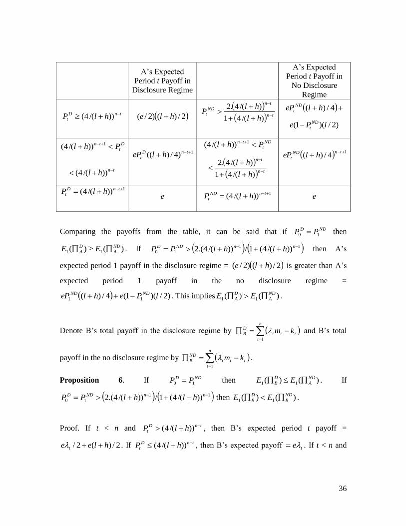
Comparing the payoffs from the table, it can be said that if NDD PP 10 then

)()( 11

ND

A

D

A EE . If 11

10 ))/(4(1/))/(4.(2 nnNDD hlhlPP then A‟s

expected period 1 payoff in the disclosure regime = 2/)()2/( hle is greater than A‟s

expected period 1 payoff in the no disclosure regime =

)2/)(1(4/)( 11 lPehleP NDND . This implies )()( 11

ND

A

D

A EE .

Denote B‟s total payoff in the disclosure regime by

n

t

ttt

D

B km1

and B‟s total

payoff in the no disclosure regime by

n

t

ttt

ND

B km1

.

Proposition 6. If NDD PP 10 then )()( 11

ND

A

D

B EE . If

11

10 ))/(4(1/))/(4.(2 nnNDD hlhlPP then )()( 11

ND

B

D

B EE .

Proof. If t < n and tnD

t hlP ))/(4( , then B‟s expected period t payoff =

2/)(2/ hlee t . If tnD

t hlP ))/(4( , then B‟s expected payoff te . If t < n and

A‟s Expected

Period t Payoff in

Disclosure Regime

A‟s Expected

Period t Payoff in

No Disclosure

Regime

tnD

t hlP ))/(4( 2/)()2/( hle

tn

tn

ND

thl

hlP

)/(41

)/(4.2

4/)( hleP ND

t

)2/)(1( lPe ND

t

D

t

tn Phl 1))/(4(

tnhl ))/(4(

1)4/)(( tnD

t hleP

ND

t

tn Phl 1))/(4(

tn

tn

hl

hl

)/(41

)/(4.2

14/)(

tnND

t hleP

1))/(4( tnD

t hlP

e

1))/(4( tnND

t hlP e

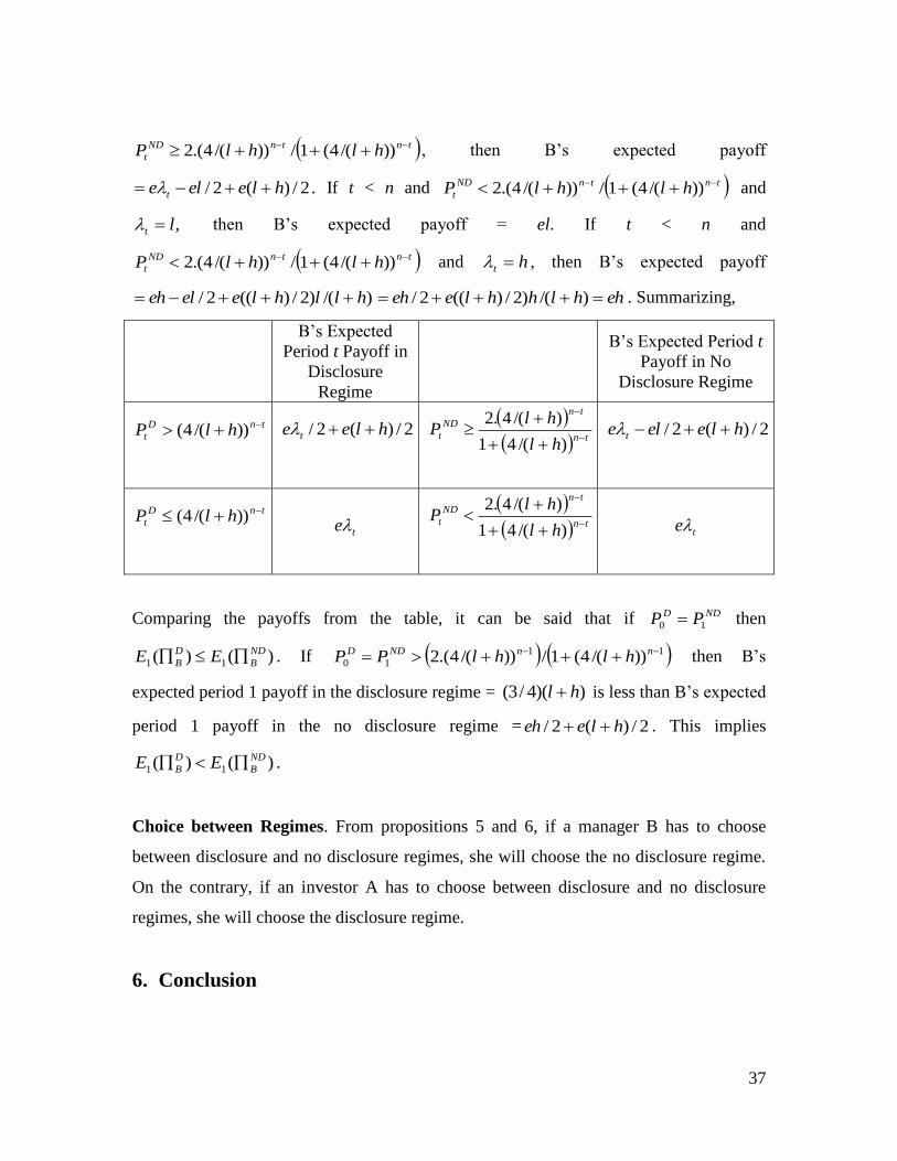
37

tntnND

t hlhlP ))/(4(1/))/(4.(2 , then B‟s expected payoff

2/)(2/ hleele t . If t < n and tntnND

t hlhlP ))/(4(1/))/(4.(2 and

,lt

then B‟s expected payoff = el. If t < n and

tntnND

t hlhlP ))/(4(1/))/(4.(2 and ht , then B‟s expected payoff

)/()2/)((2/ hllhleeleh ehhlhhleeh )/()2/)((2/ . Summarizing,

B‟s Expected

Period t Payoff in

Disclosure

Regime

B‟s Expected Period t

Payoff in No

Disclosure Regime

tnD

t hlP ))/(4(

2/)(2/ hlee t

tn

tn

ND

thl

hlP

)/(41

)/(4.2

2/)(2/ hleele t

tnD

t hlP ))/(4(

te

tn

tn

ND

thl

hlP

)/(41

)/(4.2

te

Comparing the payoffs from the table, it can be said that if NDD PP 10

then

)()( 11

ND

B

D

B EE . If 11

10 ))/(4(1/))/(4.(2 nnNDD hlhlPP then B‟s

expected period 1 payoff in the disclosure regime = ))(4/3( hl is less than B‟s expected

period 1 payoff in the no disclosure regime = 2/)(2/ hleeh . This implies

)()( 11

ND

B

D

B EE .

Choice between Regimes. From propositions 5 and 6, if a manager B has to choose

between disclosure and no disclosure regimes, she will choose the no disclosure regime.

On the contrary, if an investor A has to choose between disclosure and no disclosure

regimes, she will choose the disclosure regime.

6. Conclusion

38

This paper examines how financial disclosure enhances the building of trust and

trustworthiness to facilitate institutions for exchange and investment in complex

economic settings where there is separation of ownership and control of key economic

resources. In a setting with trustworthy and rational managers, choosing to disclose

voluntarily is a natural act of the trustworthy manager which the rational manager mimics

to receive additional future investments. However, a sequential equilibrium predicts that

such mimicking will switch from being indiscriminate (or perfect) to selective in order to

allow the rational manager to develop a reputation for being trustworthy. That is, a

manager will find it optimal to use a strategy of selective disclosure over a strategy of full

or perfect disclosure.

Disclosure and the concomitant credibility allow for a greater time of indiscriminate

mimicking and in this sense, the institution of disclosure provides reputation building

opportunities over and above those provided by the institution of dividend payment.

Characteristic features of the period of perfect mimicking are higher probability of

investment and higher probability of high returns on investment. By allowing for a

greater time of perfect mimicking, disclosure results in greater investor-manager trust,

higher investment and higher return.

While a manager‟s payoff will be higher in a world without disclosure, an investor‟s

payoff will be higher in a world with disclosure. This implies that while a manager will

prefer a world without disclosure, an investor will prefer a world with disclosure.

Given the complicated nature of the equilibrium described here, it is natural to ask if

people actually behave as predicted and this calls for an empirical examination in future

work. While disclosure has been argued to be a managerial talent signaling device, this

paper abstracts away from this question to focus on reputation building. An unanswered

question then is the role reputation building may play where managers have different

abilities in that a better manager has a higher probability of obtaining the high yield.

39

References

Angeletos, G. and A. Pavan, 2004. Transparency of Information and Co-ordination in

Economies with Investment Complementarities. American Economic Review 94(2): 91 –

98 (2004).

Arrow, K., 1972. Gifts and Exchanges. Philosophy and Public Affairs, 1972, 1 pp. 343 –

62.

Basu, S. and G. Waymire, 2006. Recordkeeping and Human Evolution. Accounting

Horizons 20(3): 201 – 229.

Basu, S., J. Dickhaut., G. Hecht, K. Towry, and G. Waymire, 2009. Recordkeeping Alters

Economic History by Promoting Reciprocity. Proceedings of the National Academy of

Sciences, 2009 106: 1009-1014.

Berg, J., J. Dickhaut and K. McCabe, 1995. Trust, Reciprocity and Social History. Games

and Economic Behavior 10(1): 122 – 142.

Bloomfield, R., 1996. Prices, Quotes and Estimates in a Laboratory Market. Journal of

Finance Vol. 51, No. 5 (Dec., 1996), pp. 1791 – 1808.

Bloomfield and Libby, 1996. Market Reactions to Differentially Available Information in

the Laboratory. Journal of Accounting Research Vol. 34, No.2 (Autumn, 1996), pp. 183 –

207.

Bushman R. and A. Smith, 2001. Financial Accounting Information and Corporate

Governance. Journal of Accounting and Economics 32 (2001) 237 – 333.

40

Camerer, C. and K. Weigelt, 1988. Experimental Tests of a Sequential Equilibrium

Reputation Model. Econometrica 56(1): 1-36.

Core, J. E., 2001. A Review of the Empirical Disclosure Literature: Discussion. Journal

of Accounting and Economics 31 (2001) 441 – 456.

Dickhaut, J., J. Hubbard, R. Lunawat and K. McCabe, 2008. Trust, Reciprocity, and

Interpersonal History: Fool me Once, Shame on You, Fool me Twice, Shame on Me.

Working paper, University of Minnesota and George Mason University.

Dickhaut, J., R. Lunawat, G. Waymire and B. Xin, 2008. Universal Adoption of Income

Reporting. Working paper, University of Minnesota, Emory University and University of

Toronto.

Dye, R., 1985a. Disclosure of Nonproprietary Information. Journal of Accounting

Research 23, 123 – 145.

Dye, Ronald A., 2001. An Evaluation of “Essays on Disclosure” and the Disclosure

Literature in Accounting. Journal of Accounting and Economics, Volume 32, Issues 1-3,

December 2001, 181 – 223.

Fukuyama, F., 1995. Trust: The Social Virtues and the Creation of Prosperity. New York:

Free Press, 1995.

Glaeser, E., D. Laibson, J.A. Scheinkman and C.L. Soutter, 2000. Measuring Trust.

Quarterly Journal of Economics 115(3): 811 – 846.

41

Grossman, S., 1981. The Informational Role of Warranties and Private Disclosure about

Product Quality. Journal of Law and Economics 24, 461 – 484.

Guiso, L., P. Sapienza and L. Zingales, 2004. The Role of Social Capital in Financial

Development. The American Economic Review, Vol. 94, No. 3 (Jun., 2004), pp. 526 –

556.

Healy, P.M. and K.G. Palepu, 1993. The Effects of Firms‟ Financial Disclosure

Strategies on Stock Prices. Accounting Horizons 7 (March): 1 – 11.

Healy, P.M. and K.G. Palepu, 2001. Information Asymmetry, Corporate Disclosure, and

the Capital markets: A Review of the Empirical Disclosure Literature. Journal of

Accounting and Economics 31 (2001) 405 – 440.

Jamal K., M. Maier and S. Sunder, 2005. Enforced Standards Versus Evolution by

General Acceptance: A Comparative Study of E-Commerce Privacy Disclosure and

Practice in the United States and the United Kingdom. Journal of Accounting Research,

Volume 43, Issue 1, pp. 73–96.

Kanodia, C. 2006. Accounting Disclosure and Real Effects. Foundations and Trends in

Accounting, Volume 1, No. 3, pp 167 – 258.

King, R. 1996. Reputation Formation for Reliable Reporting: An Experimental

Investigation. The Accounting Review 71(3): 375 – 396.

King, R. and D. Wallin, 1991a. Voluntary Disclosure when a Seller‟s Level of

Information is Unknown. Journal of Accounting Research 29: 96 – 108.

42

King, R. and D. Wallin, 1995. Experimental Tests of Disclosure with an Opponent.

Journal of Accounting and Economics 19: 139 – 168.

Knack, S. and P. Keefer, 1997. Does Social Capital Have an Economic Payoff? Cross

Country Investigation. Quarterly Journal of Economics, November 1997, 112(4), p. 1251.

Kreps, D. M. and R. Wilson, 1982. Reputation and Imperfect Information. Journal of

Economic Theory 27, 253 – 279.

Kreps, D.M., P. Milgrom, J. Roberts, and R. Wilson, 1982. Rational Cooperation in the

Finitely Repeated Prisoners‟ Dilemma. Journal of Economic Theory 27, 245 – 252.

LaPorta, R., F. Lopez de Silanes, A. Shleifer and R. Vishny, 1997. Trust in Large

Organizations. American Economic Review, May 1997b, (Papers and Proceedings),

87(2), pp. 333 – 38.

Leuz, C. and P. Wysocki, 2008. Economic Consequences of Financial Reporting and

Disclosure Regulation: A Review and Suggestions for Future Research, University of

Chicago Working paper.

McCabe, K., S. Rassenti and V. Smith, 1996. Game Theory and Reciprocity in Some

Extensive Form Experimental Games. Proceedings of the National Academy of Sciences,

Vol. 93, pp. 13421 – 13428, November 1996, Economic Sciences.

Morris, S. and H. S. Shin, 2002. Social Value of Public Information. American Economic

Review 92 (2002) (5) pp. 1521 – 1534 (December).

Putnam, R., 1993. Making Democracy Work: Civic Traditions in Modern Italy.

Princeton, NJ: Princeton University Press, 1993.

43

Sapienza, P. and L. Zingales, 2009. A Trust Crisis. Working paper, University of

Chicago.

Sapienza, P., A. Toldra and L. Zingales, 2007. Understanding Trust. NBER Working

Paper No. 13387.

Solow, R., 1995. Trust: The Social Virtues and the Creation of Prosperity (Book

Review). New Republic, 1995, 213, pp. 36 – 40.

Verrecchia, R. E., 2001. Essays on Disclosure. Journal of Accounting and Economics,

Volume 32, Issues 1-3, December 2001, 97 – 180.