Reproducible Research Tools for R

1

January 2017

Boriana Pratt

Princeton University

Literate programming

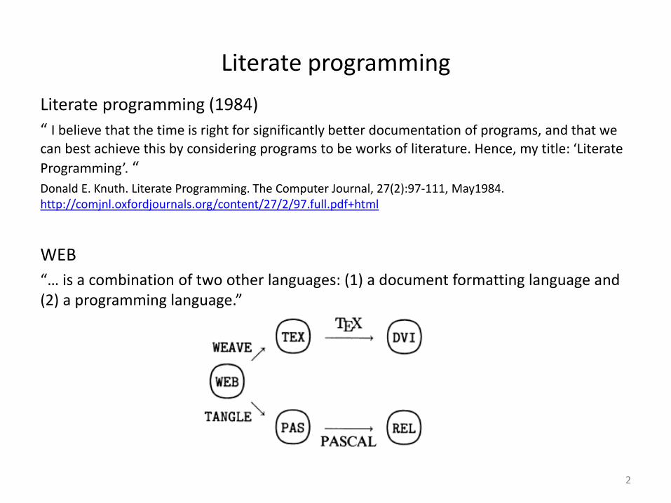
Literate programming (1984)

“ I believe that the time is right for significantly better documentation of programs, and that we can best achieve this by considering programs to be works of literature. Hence, my title: ‘Literate

Programming’. “ Donald E. Knuth. Literate Programming. The Computer Journal, 27(2):97-111, May1984. http://comjnl.oxfordjournals.org/content/27/2/97.full.pdf+html

WEB

“… is a combination of two other languages: (1) a document formatting language and (2) a programming language.”

2

terms

• Tangle

extract the code parts (code chunks), then run them sequentially

• Weave

extract the text part (documentation chunks) and weave back in the code and code output

3

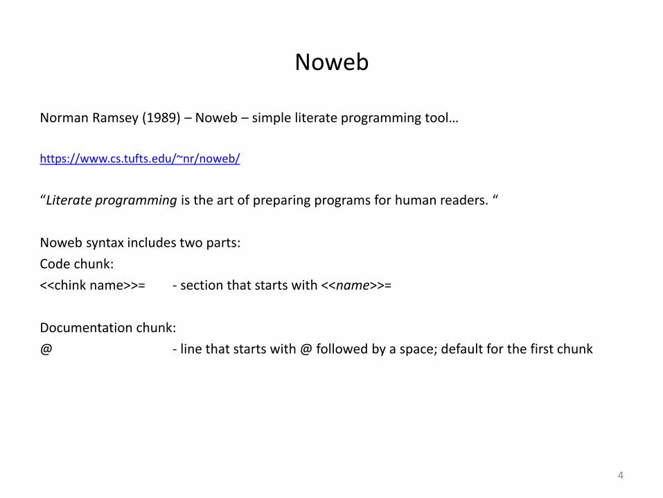
Noweb

Norman Ramsey (1989) – Noweb – simple literate programming tool…

https://www.cs.tufts.edu/~nr/noweb/

“Literate programming is the art of preparing programs for human readers. “

Noweb syntax includes two parts:

Code chunk:

<<chink name>>= - section that starts with <<name>>=

Documentation chunk:

@ - line that starts with @ followed by a space; default for the first chunk

4

Tools for R

5

Tools for R

• Sweave https://stat.ethz.ch/R-manual/R-devel/library/utils/doc/Sweave.pdf

What is Sweave?

A tool that allows to embed the R code in LaTeX documents. The purpose is to create dynamic reports, which can be updated automatically if data or analysis change.

How do I cite Sweave?

To cite Sweave please use the paper describing the first version:

Friedrich Leisch. Sweave: Dynamic generation of statistical reports using literate data analysis. In W. Härdle and B. Rönz, editors, Compstat 2002 – Proceedings in Computational Statistics, pages 575-580. Phisica Verlag, Heidelberg, 2002.

6

Tools for R

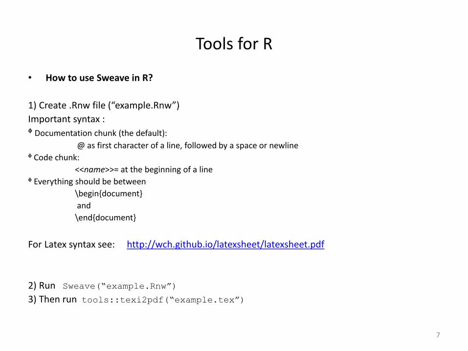
• How to use Sweave in R?

1) Create .Rnw file (“example.Rnw”)

Important syntax :

ᶲ Documentation chunk (the default):

@ as first character of a line, followed by a space or newline

ᶲ Code chunk:

<<name>>= at the beginning of a line

ᶲ Everything should be between

\begin{document}

and

\end{document}

For Latex syntax see: http://wch.github.io/latexsheet/latexsheet.pdf

2) Run Sweave(“example.Rnw”)

3) Then run tools::texi2pdf(“example.tex”)

7

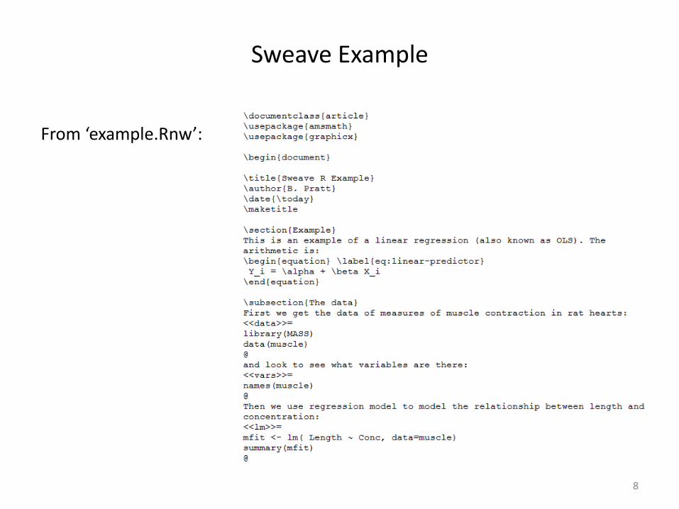
Sweave Example

From ‘example.Rnw’:

8

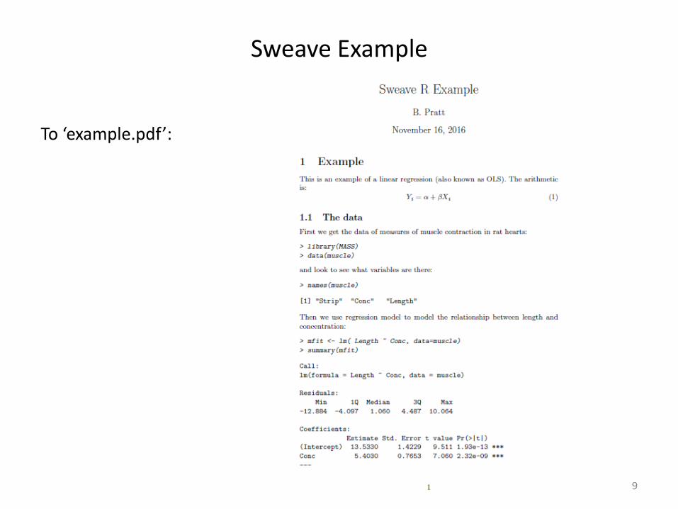
Sweave Example

To ‘example.pdf’:

9

Sweave Example

• in Rstudio: File > New File > R Sweave

try it…

10

Tools for R

• Knitr http://yihui.name/knitr/demo/manual/

http://yihui.name/knitr/demo/graphics/

Knitr is an R package that enables integration of R code

into LaTeX, LyX, HTML and other documents.

You write the R code in ‘code chunks’.

Code chunks are between ``` and ```.

Knitr package on GitHub: https://github.com/yihui/knitr

11

knitr Setting global option for the all code chunks:

```{r global_options, include = FALSE}

knitr:: opts_chunk$set(fig.width = 12, fig.height = 8, echo = FALSE, |

warning = FALSE, message = FALSE)

```

Options to use for code chunks:

12

Tools for R

Rmarkdown ( Yihui Xie, 2014) From http://rmarkdown.rstudio.com/authoring_quick_tour.html :

“ Markdown is a simple formatting language designed to make authoring content easy for everyone. Rather than write in complex markup code (e.g. HTML or LaTex), you write in plain text with formatting cues. Pandoc uses these cues to turn your document into attractive output. “

How it works: 1. Create an .Rmd file that contains a combination of markdown and R code chunks.

2. The .Rmd file is fed to knitr, which executes all of the R code chunks and creates a new markdown (.md) document which includes the R code and it’s output.

3. The .md file is then processed by pandoc, which creates a finished web page, PDF, MS Word document, slide show, handout, book, dashboard, package vignette or other format.

For pandoc file formats, see here: http://pandoc.org/

13

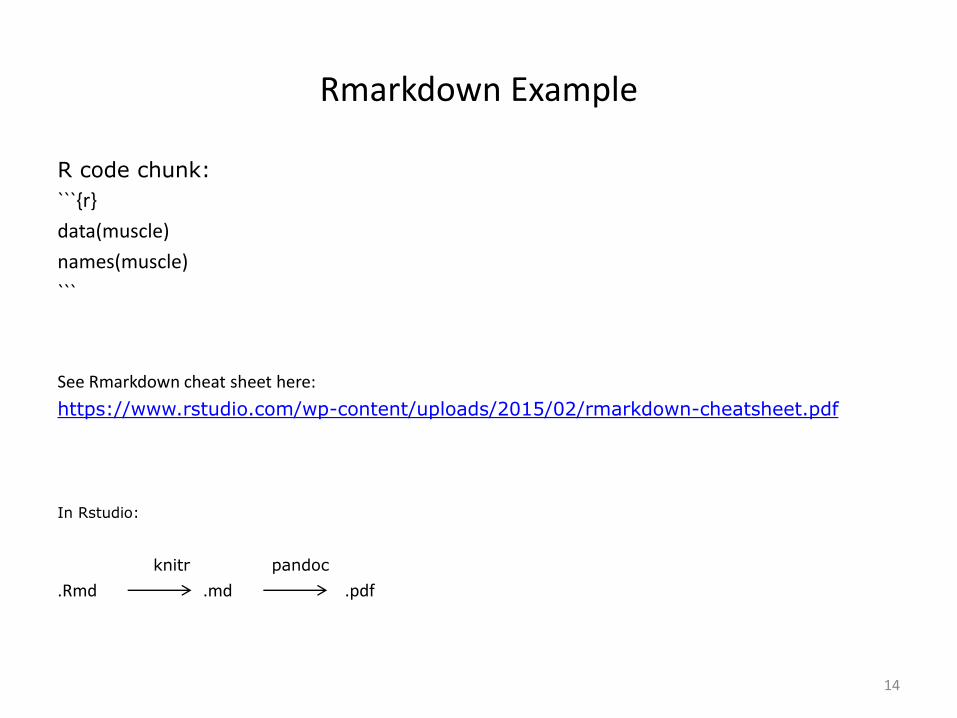
Rmarkdown Example

R code chunk:

```{r}

data(muscle)

names(muscle)

```

See Rmarkdown cheat sheet here:

https://www.rstudio.com/wp-content/uploads/2015/02/rmarkdown-cheatsheet.pdf

In Rstudio:

knitr pandoc

.Rmd .md .pdf

14

Rmarkdown in R

To run Rmarkdown in R (requires pandoc to be installed) :

install.packages(“rmarkdown”)

library(rmarkdown)

render(“example.Rmd”)

Default output is .pdf, could specify html: render(“example.Rmd”,html_document())

15

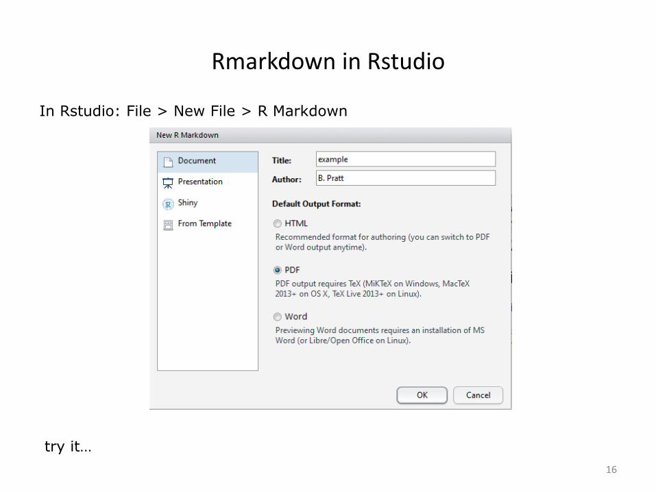
Rmarkdown in Rstudio

In Rstudio: File > New File > R Markdown

try it…

16

Top part is a YAML header. YAML is data serialization language.

For more on YAML, see: http://yaml.org/spec/1.0/

Rmarkdown in Rstudio

17

Rmarkdown in Rstudio

Let’s try to:

1.add a sentence

2. add a header

3. add a code chunk

Example code chunk: ```{r}

a <- 1:10

a

```

Some code chunk options:

```{r chunk_name, echo=FALSE, include=TRUE} – do not display code in output document

```{r scatter, fig.width=8, fig.height=6} – set size for figure

```{r, include=FALSE} – do not include output from this chunk

18

Rmarkdown in Rstudio

Inline Expressions: The sum of three, five and eight is `r 3+5+8`.

Result:

The sum of three, five and eight is 16.

Regression table: ```{r, results=„asis‟}

library(knitr)

n <- 100

x <- rnorm(n)

y <- 2*x + rnorm(n)

out <- lm(y ~ x)

kable(summary(out)$coef, digits=2)

```

Try to:

. add to your .Rmd file a plot, then re-size it using the chunk options

. add to your .Rmd file an inline expression

. add a regression table (could use package xtable)

19

R Notebook

In Rstudio (the newest version) go to File -> New File -> R Notebook to create a R Notebook file, which is a Rmarkdown file, accompanied by a .nb (notebook) file which could be previewed in a browser.

20

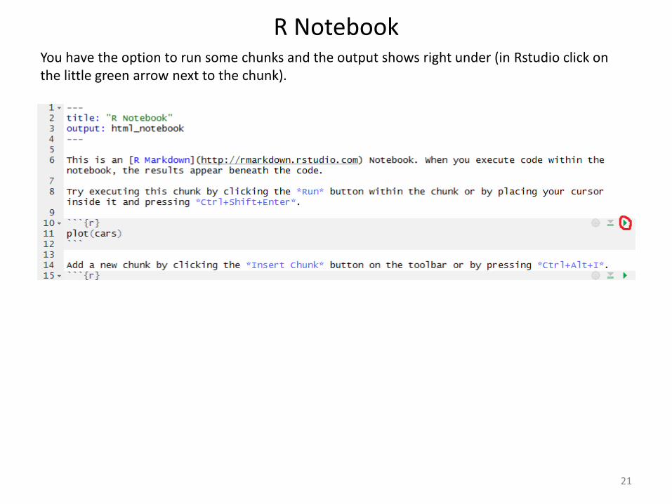
R Notebook You have the option to run some chunks and the output shows right under (in Rstudio click on the little green arrow next to the chunk).

21

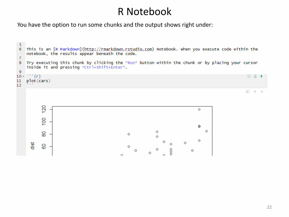
R Notebook You have the option to run some chunks and the output shows right under:

22

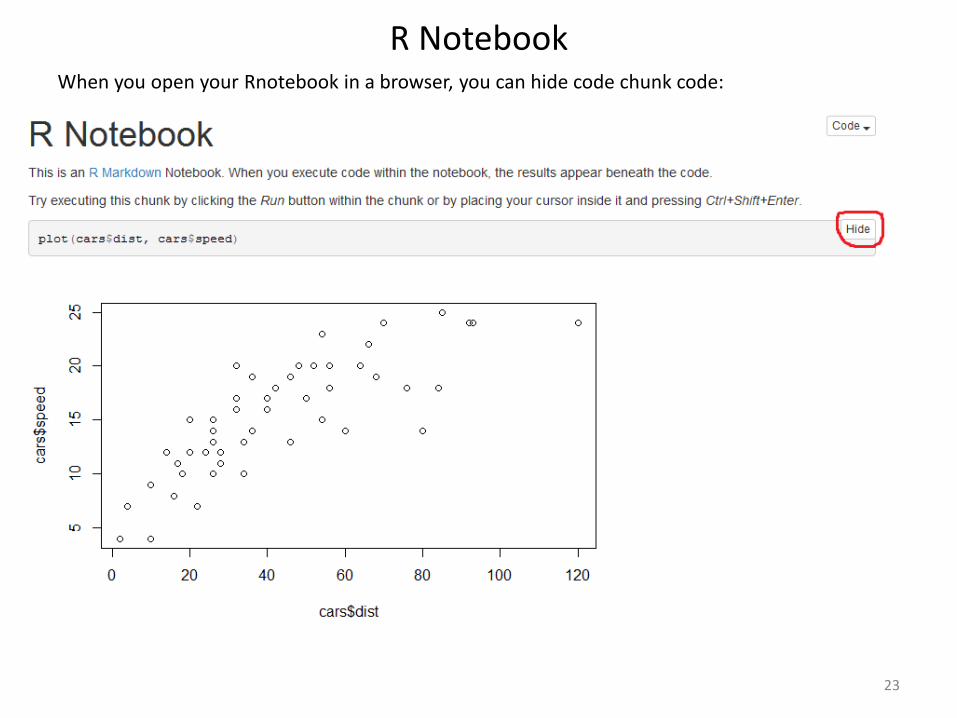
R Notebook When you open your Rnotebook in a browser, you can hide code chunk code:

23

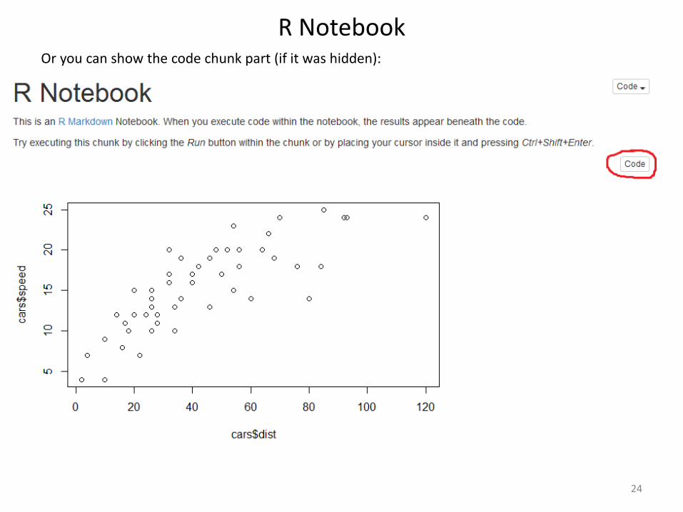
R Notebook Or you can show the code chunk part (if it was hidden):

24

R Notebook You can hide all code chunks and only leave the output visible:

25

Thank you.

26