Representations of Ordinal Numbers · number. I The successor of an ordinal number is an ordinal...
45
Representations of Ordinal Numbers Juan Sebasti´ an C´ ardenas-Rodr´ ıguez Andr´ es Sicard-Ram´ ırez * Mathematical Engineering, Universidad EAFIT September 19, 2019 * Tutor
Transcript of Representations of Ordinal Numbers · number. I The successor of an ordinal number is an ordinal...
Representations of Ordinal Numbers
Juan Sebastian Cardenas-Rodrıguez
Andres Sicard-Ramırez∗
Mathematical Engineering, Universidad EAFIT
September 19, 2019
∗Tutor
Ordinal numbersCantor
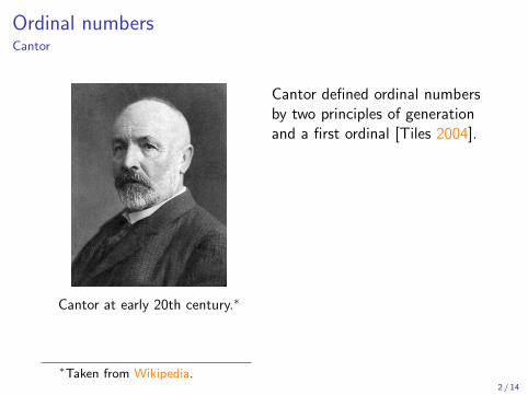
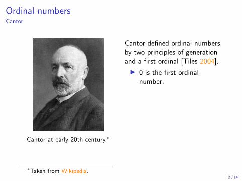
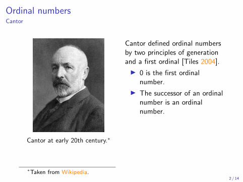
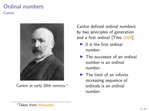
Cantor at early 20th century.∗
Cantor defined ordinal numbersby two principles of generationand a first ordinal [Tiles 2004].
I 0 is the first ordinalnumber.
I The successor of an ordinalnumber is an ordinalnumber.
I The limit of an infiniteincreasing sequence ofordinals is an ordinalnumber.
∗Taken from Wikipedia.2 / 14
Ordinal numbersCantor
Cantor at early 20th century.∗
Cantor defined ordinal numbersby two principles of generationand a first ordinal [Tiles 2004].
I 0 is the first ordinalnumber.
I The successor of an ordinalnumber is an ordinalnumber.
I The limit of an infiniteincreasing sequence ofordinals is an ordinalnumber.
∗Taken from Wikipedia.2 / 14
Ordinal numbersConstructing Some Ordinals
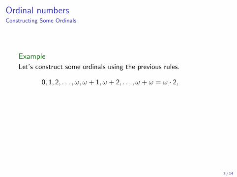
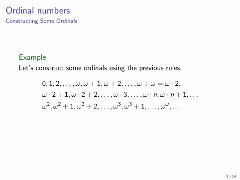
Example
Let’s construct some ordinals using the previous rules.
0, 1, 2, . . . , ω, ω + 1, ω + 2, . . . , ω + ω = ω · 2,ω · 2 + 1, ω · 2 + 2, . . . , ω · 3, . . . , ω · n, ω · n + 1, . . .
ω2, ω2 + 1, ω2 + 2, . . . , ω3, ω3 + 1, . . . , ωω, . . .
ωωω, . . . , ωωωω
, . . . , ωωωωω
, . . . , ε0, . . .
3 / 14
Ordinal numbersConstructing Some Ordinals
Example
Let’s construct some ordinals using the previous rules.
0, 1, 2, . . . , ω, ω + 1, ω + 2, . . . , ω + ω = ω · 2,
ω · 2 + 1, ω · 2 + 2, . . . , ω · 3, . . . , ω · n, ω · n + 1, . . .
ω2, ω2 + 1, ω2 + 2, . . . , ω3, ω3 + 1, . . . , ωω, . . .
ωωω, . . . , ωωωω
, . . . , ωωωωω
, . . . , ε0, . . .
3 / 14

Ordinal numbersConstructing Some Ordinals
Example
Let’s construct some ordinals using the previous rules.
0, 1, 2, . . . , ω, ω + 1, ω + 2, . . . , ω + ω = ω · 2,ω · 2 + 1, ω · 2 + 2, . . . , ω · 3, . . . , ω · n, ω · n + 1, . . .
ω2, ω2 + 1, ω2 + 2, . . . , ω3, ω3 + 1, . . . , ωω, . . .
ωωω, . . . , ωωωω
, . . . , ωωωωω
, . . . , ε0, . . .
3 / 14
Ordinal numbersConstructing Some Ordinals
Example
Let’s construct some ordinals using the previous rules.
0, 1, 2, . . . , ω, ω + 1, ω + 2, . . . , ω + ω = ω · 2,ω · 2 + 1, ω · 2 + 2, . . . , ω · 3, . . . , ω · n, ω · n + 1, . . .
ω2, ω2 + 1, ω2 + 2, . . . , ω3, ω3 + 1, . . . , ωω, . . .
ωωω, . . . , ωωωω
, . . . , ωωωωω
, . . . , ε0, . . .
3 / 14
Ordinal numbersvon Neumann Ordinals
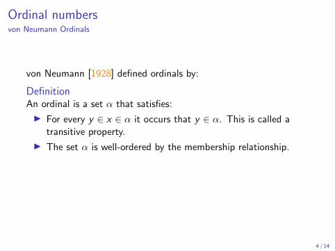
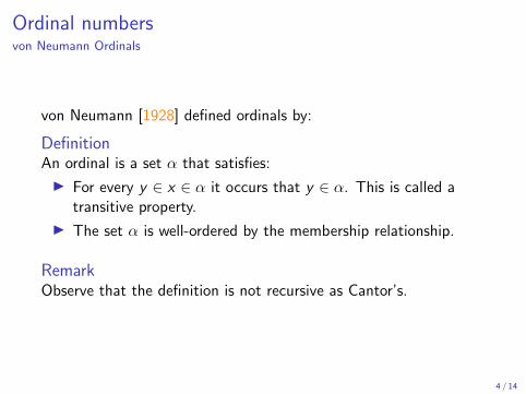
von Neumann [1928] defined ordinals by:
DefinitionAn ordinal is a set α that satisfies:
I For every y ∈ x ∈ α it occurs that y ∈ α. This is called atransitive property.
I The set α is well-ordered by the membership relationship.
RemarkObserve that the definition is not recursive as Cantor’s.
4 / 14
Ordinal numbersvon Neumann Ordinals
von Neumann [1928] defined ordinals by:
DefinitionAn ordinal is a set α that satisfies:
I For every y ∈ x ∈ α it occurs that y ∈ α. This is called atransitive property.
I The set α is well-ordered by the membership relationship.
RemarkObserve that the definition is not recursive as Cantor’s.
4 / 14
Ordinal numbersSome von Neumann Ordinals
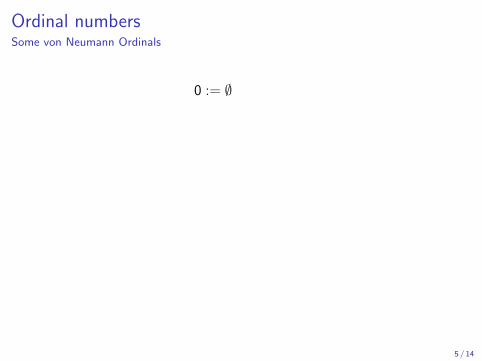
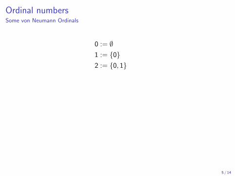
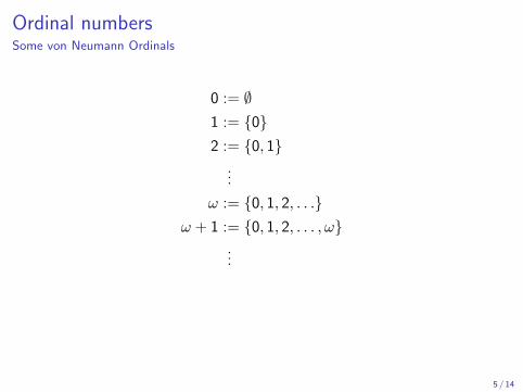
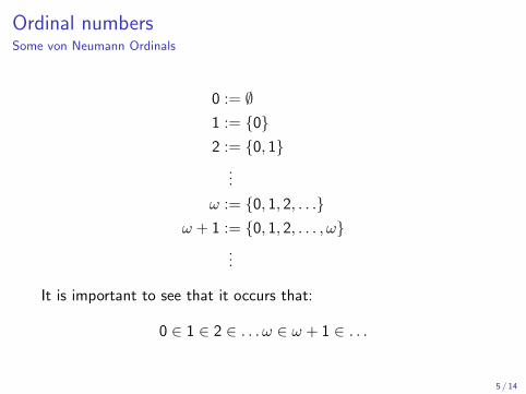
0 := ∅
1 := {0}2 := {0, 1}
...
ω := {0, 1, 2, . . .}ω + 1 := {0, 1, 2, . . . , ω}
...
It is important to see that it occurs that:
0 ∈ 1 ∈ 2 ∈ . . . ω ∈ ω + 1 ∈ . . .
5 / 14
Ordinal numbersSome von Neumann Ordinals
0 := ∅1 := {0}2 := {0, 1}
...
ω := {0, 1, 2, . . .}ω + 1 := {0, 1, 2, . . . , ω}
...
It is important to see that it occurs that:
0 ∈ 1 ∈ 2 ∈ . . . ω ∈ ω + 1 ∈ . . .
5 / 14
Ordinal numbersSome von Neumann Ordinals
0 := ∅1 := {0}2 := {0, 1}
...
ω := {0, 1, 2, . . .}ω + 1 := {0, 1, 2, . . . , ω}
...
It is important to see that it occurs that:
0 ∈ 1 ∈ 2 ∈ . . . ω ∈ ω + 1 ∈ . . .
5 / 14
Ordinal numbersSome von Neumann Ordinals
0 := ∅1 := {0}2 := {0, 1}
...
ω := {0, 1, 2, . . .}ω + 1 := {0, 1, 2, . . . , ω}
...
It is important to see that it occurs that:
0 ∈ 1 ∈ 2 ∈ . . . ω ∈ ω + 1 ∈ . . .
5 / 14
Ordinal numbersCountable Ordinals
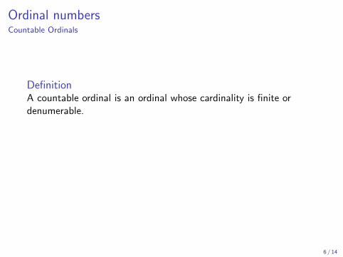
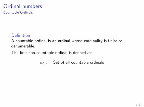
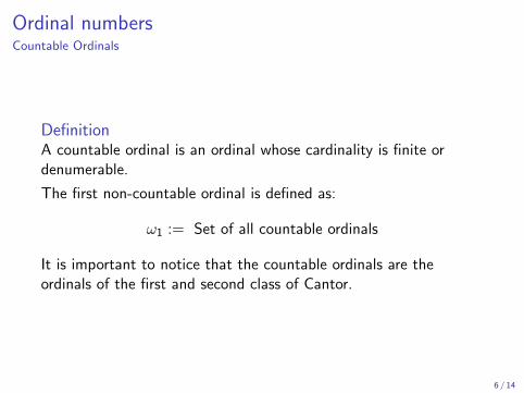
DefinitionA countable ordinal is an ordinal whose cardinality is finite ordenumerable.
The first non-countable ordinal is defined as:
ω1 := Set of all countable ordinals
It is important to notice that the countable ordinals are theordinals of the first and second class of Cantor.
6 / 14
Ordinal numbersCountable Ordinals
DefinitionA countable ordinal is an ordinal whose cardinality is finite ordenumerable.
The first non-countable ordinal is defined as:
ω1 := Set of all countable ordinals
It is important to notice that the countable ordinals are theordinals of the first and second class of Cantor.
6 / 14
Ordinal numbersHilbert Definition
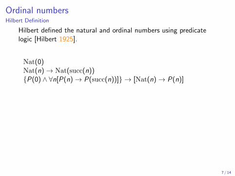
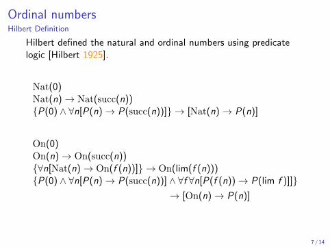
Hilbert defined the natural and ordinal numbers using predicatelogic [Hilbert 1925].
Nat(0)Nat(n)→ Nat(succ(n)){P(0) ∧ ∀n[P(n)→ P(succ(n))]} → [Nat(n)→ P(n)]
On(0)On(n)→ On(succ(n)){∀n[Nat(n)→ On(f (n))]} → On(lim(f (n))){P(0) ∧ ∀n[P(n)→ P(succ(n))] ∧ ∀f ∀n[P(f (n))→ P(lim f )]]}
→ [On(n)→ P(n)]
where Nat and On are propositional functions representing bothnumbers.
7 / 14
Ordinal numbersHilbert Definition
Hilbert defined the natural and ordinal numbers using predicatelogic [Hilbert 1925].
Nat(0)Nat(n)→ Nat(succ(n)){P(0) ∧ ∀n[P(n)→ P(succ(n))]} → [Nat(n)→ P(n)]
On(0)On(n)→ On(succ(n)){∀n[Nat(n)→ On(f (n))]} → On(lim(f (n))){P(0) ∧ ∀n[P(n)→ P(succ(n))] ∧ ∀f ∀n[P(f (n))→ P(lim f )]]}
→ [On(n)→ P(n)]
where Nat and On are propositional functions representing bothnumbers.
7 / 14
Ordinal numbersComputable Ordinals
Church and Kleene [1937] defined computable ordinals as ordinalsthat are λ-definable.
RemarkThe computable ordinals are less than the countable ones, as thereare less λ-terms than real numbers.
The first countable ordinal that is non-computable is called ωCK1
∗.Furthermore, all non-countable ordinals are non-computable.
∗See CK Wikipedia8 / 14
Ordinal numbersComputable Ordinals
Church and Kleene [1937] defined computable ordinals as ordinalsthat are λ-definable.
RemarkThe computable ordinals are less than the countable ones, as thereare less λ-terms than real numbers.
The first countable ordinal that is non-computable is called ωCK1
∗.
Furthermore, all non-countable ordinals are non-computable.
∗See CK Wikipedia8 / 14
Ordinal numbersComputable Ordinals
Church and Kleene [1937] defined computable ordinals as ordinalsthat are λ-definable.
RemarkThe computable ordinals are less than the countable ones, as thereare less λ-terms than real numbers.
The first countable ordinal that is non-computable is called ωCK1
∗.Furthermore, all non-countable ordinals are non-computable.
∗See CK Wikipedia8 / 14
RepresentationsHardy
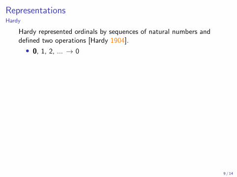
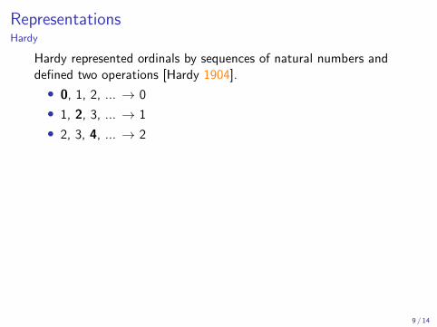
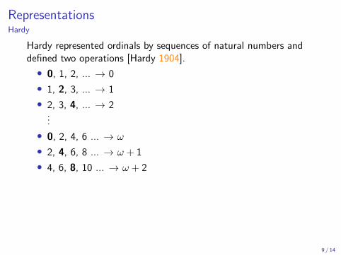
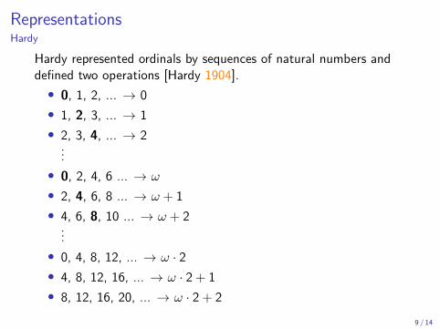
Hardy represented ordinals by sequences of natural numbers anddefined two operations [Hardy 1904].
• 0, 1, 2, ... → 0
• 1, 2, 3, ... → 1
• 2, 3, 4, ... → 2...
• 0, 2, 4, 6 ... → ω
• 2, 4, 6, 8 ... → ω + 1
• 4, 6, 8, 10 ... → ω + 2...
• 0, 4, 8, 12, ... → ω · 2• 4, 8, 12, 16, ... → ω · 2 + 1
• 8, 12, 16, 20, ... → ω · 2 + 2
9 / 14
RepresentationsHardy
Hardy represented ordinals by sequences of natural numbers anddefined two operations [Hardy 1904].
• 0, 1, 2, ... → 0
• 1, 2, 3, ... → 1
• 2, 3, 4, ... → 2
...
• 0, 2, 4, 6 ... → ω
• 2, 4, 6, 8 ... → ω + 1
• 4, 6, 8, 10 ... → ω + 2...
• 0, 4, 8, 12, ... → ω · 2• 4, 8, 12, 16, ... → ω · 2 + 1
• 8, 12, 16, 20, ... → ω · 2 + 2
9 / 14
RepresentationsHardy
Hardy represented ordinals by sequences of natural numbers anddefined two operations [Hardy 1904].
• 0, 1, 2, ... → 0
• 1, 2, 3, ... → 1
• 2, 3, 4, ... → 2...
• 0, 2, 4, 6 ... → ω
• 2, 4, 6, 8 ... → ω + 1
• 4, 6, 8, 10 ... → ω + 2
...
• 0, 4, 8, 12, ... → ω · 2• 4, 8, 12, 16, ... → ω · 2 + 1
• 8, 12, 16, 20, ... → ω · 2 + 2
9 / 14
RepresentationsHardy
Hardy represented ordinals by sequences of natural numbers anddefined two operations [Hardy 1904].
• 0, 1, 2, ... → 0
• 1, 2, 3, ... → 1
• 2, 3, 4, ... → 2...
• 0, 2, 4, 6 ... → ω
• 2, 4, 6, 8 ... → ω + 1
• 4, 6, 8, 10 ... → ω + 2...
• 0, 4, 8, 12, ... → ω · 2• 4, 8, 12, 16, ... → ω · 2 + 1
• 8, 12, 16, 20, ... → ω · 2 + 2
9 / 14
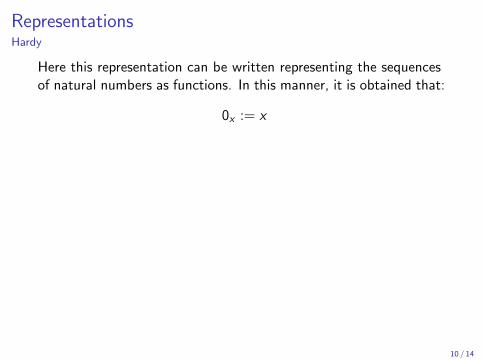
RepresentationsHardy
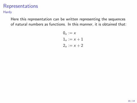
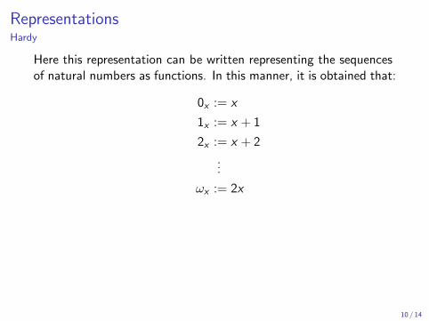
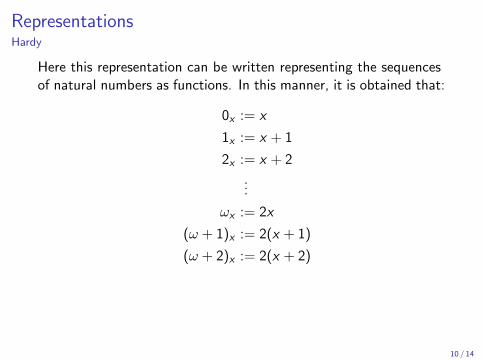
Here this representation can be written representing the sequencesof natural numbers as functions. In this manner, it is obtained that:
0x := x
1x := x + 1
2x := x + 2
...
ωx := 2x
(ω + 1)x := 2(x + 1)
(ω + 2)x := 2(x + 2)
...
(ω · n + k)x := 2n(x + k)
10 / 14
RepresentationsHardy
Here this representation can be written representing the sequencesof natural numbers as functions. In this manner, it is obtained that:
0x := x
1x := x + 1
2x := x + 2
...
ωx := 2x
(ω + 1)x := 2(x + 1)
(ω + 2)x := 2(x + 2)
...
(ω · n + k)x := 2n(x + k)
10 / 14
RepresentationsHardy
Here this representation can be written representing the sequencesof natural numbers as functions. In this manner, it is obtained that:
0x := x
1x := x + 1
2x := x + 2
...
ωx := 2x
(ω + 1)x := 2(x + 1)
(ω + 2)x := 2(x + 2)
...
(ω · n + k)x := 2n(x + k)
10 / 14
RepresentationsHardy
Here this representation can be written representing the sequencesof natural numbers as functions. In this manner, it is obtained that:
0x := x
1x := x + 1
2x := x + 2
...
ωx := 2x
(ω + 1)x := 2(x + 1)
(ω + 2)x := 2(x + 2)
...
(ω · n + k)x := 2n(x + k)
10 / 14
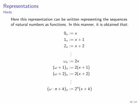
RepresentationsHardy
Here this representation can be written representing the sequencesof natural numbers as functions. In this manner, it is obtained that:
0x := x
1x := x + 1
2x := x + 2
...
ωx := 2x
(ω + 1)x := 2(x + 1)
(ω + 2)x := 2(x + 2)
...
(ω · n + k)x := 2n(x + k)
10 / 14
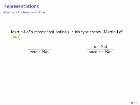
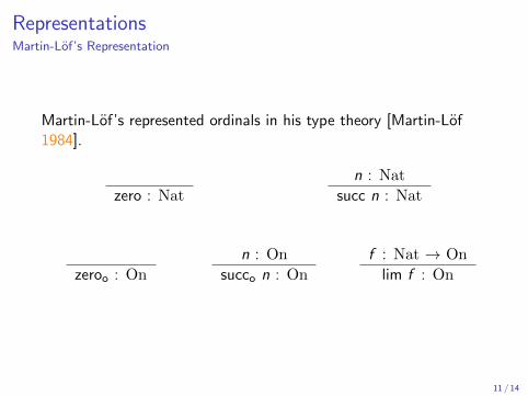
RepresentationsMartin-Lof’s Representation
Martin-Lof’s represented ordinals in his type theory [Martin-Lof1984].
zero : Nat
n : Nat
succ n : Nat
zeroo : On
n : On
succo n : On
f : Nat → On
lim f : On
11 / 14
RepresentationsMartin-Lof’s Representation
Martin-Lof’s represented ordinals in his type theory [Martin-Lof1984].
zero : Nat
n : Nat
succ n : Nat
zeroo : On
n : On
succo n : On
f : Nat → On
lim f : On
11 / 14
RepresentationsMartin-Lof’s Representation
Martin-Lof’s represented ordinals in his type theory [Martin-Lof1984].
zero : Nat
n : Nat
succ n : Nat
zeroo : On
n : On
succo n : On
f : Nat → On
lim f : On
11 / 14
RepresentationsMartin-Lof’s Representation
RemarkMartin-Lof’s definition is analogous to Cantor and Hilbert’sdefinition.
QuestionWhich ordinal cannot be constructed by Martin-Lof’srepresentation?
Is it possible to define, similarly, a ωML1 ?
12 / 14

RepresentationsMartin-Lof’s Representation
RemarkMartin-Lof’s definition is analogous to Cantor and Hilbert’sdefinition.
QuestionWhich ordinal cannot be constructed by Martin-Lof’srepresentation?
Is it possible to define, similarly, a ωML1 ?
12 / 14
RepresentationsMartin-Lof’s Representation
RemarkMartin-Lof’s definition is analogous to Cantor and Hilbert’sdefinition.
QuestionWhich ordinal cannot be constructed by Martin-Lof’srepresentation?
Is it possible to define, similarly, a ωML1 ?
12 / 14
References I
Church, Alonzo and Kleene (1937). “Formal Definitions inthe Theory of Ordinal Numbers”. In: FundamentaMathematicae 28, pp. 11–21.Hardy, Godfrey H. (1904). “A Theorem Concerning theInfinite Cardinal Numbers”. In: Quarterly Journal ofMathematics 35, pp. 87–94.Hilbert, David (1925). “On the Infinite”. In: Reprinted in:From Frege to Godel: A Source Book in Mathematical Logic,1879-1931 (1967). Ed. by Jean van Heijenoort. Vol. 9.Harvard University Press, pp. 367–392.Martin-Lof, Per (1984). Intuitonistic Type Theory. Bibliopolis.Neumann, J. von (1928). “Die Axiomatisierung derMengenlehre”. In: Mathematische Zeitschrift 27.1,pp. 669–752.
13 / 14
References II
Tiles, Mary (2004). The Philosophy of Set Theory: AnHistorical Introduction to Cantor’s Paradise. CourierCorporation.
14 / 14


![CONSTRUCTIVE VERSIONS OF ORDINAL NUMBER CLASSES · 1961] CONSTRUCTIVE VERSIONS OF ORDINAL NUMBER CLASSES 327 to the segment of ordinals through the "third number class" (i.e. through](https://static.fdocuments.in/doc/165x107/5e8b00784c19c5021b2230fd/constructive-versions-of-ordinal-number-1961-constructive-versions-of-ordinal-number.jpg)