
Baltic containerization - Baltic Press - Baltic Transport Journal

ICES SGABC Report 2006 ICES Baltic Committee
ICES CM 2006/BCC:08
Report of the Study Group on Ageing Issues
of Baltic Cod (SGABC)
16–19 May 2006
Gdynia, Poland

International Council for the Exploration of the Sea Conseil International pour l’Exploration de la Mer H.C. Andersens Boulevard 44-46 DK-1553 Copenhagen V Denmark Telephone (+45) 33 38 67 00 Telefax (+45) 33 93 42 15 www.ices.dk [email protected]
Recommended format for purposes of citation: ICES. 2006. Report of the Study Group on Ageing Issues of Baltic Cod (SGABC), 16–19 May 2006, Gdynia, Poland. ICES CM 2006/BCC:08. 45 pp. For permission to reproduce material from this publication, please apply to the General Secretary.
The document is a report of an Expert Group under the auspices of the International Council for the Exploration of the Sea and does not necessarily represent the views of the Council.
© 2006 International Council for the Exploration of the Sea.

ICES SGABC Report 2006 | i
Contents
Executive summary......................................................................................................... 1
1 Terms of Reference.................................................................................................. 2
2 Agenda and participation........................................................................................ 2
3 Statistical and model development (ToR a, b)....................................................... 2 3.1 Methodological development .......................................................................... 2
3.1.1 Theoretical considerations .................................................................. 2 3.1.2 Modelling cod bioenergetics and otolith accretion ............................. 3 3.1.3 Effects of non-normal distribution of weight frequencies .................. 5
3.2 Considerations by WGBFAS on ageing errors................................................ 6
4 Progress in compilation of otolith weight data (ToR c)........................................ 8 4.1 State of otolith weight database....................................................................... 8 4.2 Exploration of data .......................................................................................... 8
4.2.1 Comparison of otolith weight distributions between and within countries.............................................................................................. 8
4.2.2 Relation between otolith weight and fish length in ICES Subdivisions 26 and 28....................................................................... 9
5 Age determination workshop (ToR d, e, f) .......................................................... 10 5.1 Application of image analysis in age reading calibrations ............................ 10 5.2 Exchange programs ....................................................................................... 10
5.2.1 Results .............................................................................................. 11 5.2.2 Conclusions ...................................................................................... 12
5.3 Calibration exercises during SGABC, May 2006.......................................... 12 5.3.1 Results .............................................................................................. 12 5.3.2 Conclusions ...................................................................................... 13
5.4 Age reader discussion on the distribution of O1 across areas and season ..... 13 5.5 Overall conclusion and recommendations ..................................................... 14
6 Organisation of future work ................................................................................. 16 6.1 Relevant research projects and plans ............................................................. 16 6.2 Proposal for organisational structure ............................................................. 17
7 Recommendations.................................................................................................. 18
8 References .............................................................................................................. 19
Annex 1: Agenda for the SGABC meeting in Gdynia, 16–19 May 2006.................. 41
Annex 2: List of participants ....................................................................................... 43
Annex 3: Recommendation buzzlist ............................................................................ 45


ICES SGABC Report 2006 | 1
Executive summary
A model on otolith growth in weight has been developed that relates otolith accretion rate to physical and physiological conditions. Two main factors, food and temperature, which both influence otolith growth, have been explored and mathematical expressions have been developed that conforms to bioenergetic knowledge. The model has only partly been validated since very few relevant experiments with known-age cod have been done in the Baltic.
Data on 44 494 otolith weights of cod from 1996 to 2005 have been collected and compiled in a simple database. The database also contains individual ages as well as length frequencies. The international FISHFRAME database has been reconfigured to be able to include otolith weights and some national data have already been entered. The intention is that otolith weights from research surveys should be entered into the ICES DATRAS database.
Observed otolith weight distributions arranged by reader estimates of ages have been used to infer differences in the age determination process. Results indicate large discrepancies between age readers of different countries. This has also been confirmed by exchange programmes.
A new method to calibrate between age readers has been further tested. The method combines traditional optical inspection with the use of image mapping, where age readers can identify otolith annulli and compare their own identification with that of other age readers. The method was also used to quantify differences between age readers and thereby stimulated discussions among age readers.
SGABC concludes that:
• The development of an otolith growth model is hampered by the lack of validation material (mark-recapture or other data on known age). This will prevent not only validation but also the development of statistical methods to update historical data.
• The annual and intersessional age reading exercises have not improved the precision between age readers. Still, there is a large variation in the interpretation of ages both between laboratories but also within single readers.
• Annual study groups do not provide a sufficient effort to overcome above difficulties. Instead a dedicated and focussed research programme should address the age reading problems.

2 | ICES SGABC Report 2006
1 Terms of Reference
Baltic Committee resolution 2005/2/BCC08: The Study Group on Ageing Issues of Baltic Cod [SGABC] (Chair: J. Modin, Sweden) will meet in Gdynia, Poland, from 16–19 May 2006 to:
a ) demonstrate statistical tools that can be used to calibrate otolith and fish growth and to estimate age compositions of historical data based on otolith biometrics of Baltic cod;
b ) update the otolith growth model and evaluate its usefulness for an assessment of historical age compositions of Baltic cod;
c ) report on the progress of the compilation of biometric data of Baltic cod otoliths that have been collected from research surveys, market and sea sampling in 2001 to 2005;
d ) develop and advice on the reconstruction of historical age compositions from otolith biometrics. This activity should include a plan for an update of historical otolith weight data for Baltic cod stocks;
e ) perform an in depth analysis of difference in age reader interpretation of otolith spatial patterns and explore the usage of metric measurements of otolith structures as a solution to minimize the divergence in age estimation of Baltic cod;
f ) evaluate the use of traditional age determination combined with recent development in image analysis in order to include back-calculation of length at age and growth based on age structures defined by age-readers;
g ) organise the 2006 meeting in parallel sessions, which will enable age readers to meet separately and discuss interpretations of otolith structures in view of intersessional ex-change programs. The session will be co-chaired by Lotte Worsøe Clausen, Denmark.
2 Agenda and participation
The adopted agenda is presented in Annex 1, which also contains the agenda for the sub-group session with age reader experts.
The list of participants is presented in Annex 2.
3 Statistical and model development (ToR a, b)
3.1 Methodological development
3.1.1 Theoretical considerations
Francis and Campana (2004) demonstrated that otolith weight can be used to estimate age population structure of fishes. The authors stress that the purpose of inferring age is ultimately to obtain information on proportions at age at a population level, usually from some form of stock assessment model. Hence the intention of the methodology should be to estimate proportions at age, rather than to assign ages to individual fish, which has tended to be the purpose of previous work on the use of otolith measurements. The authors also note that the normal procedure for age-determination by otolith size distributions will be to work from a relatively small ‘calibration sample’ for which relatively detailed information on age proportions has been obtained, then use this to estimate the proportions at age for a larger ‘production sample’ for which only limited information is available. A short overview of their discussion is available in the SGABC (2006, Section 3.1).
The approach has been further examined by Francis et al. (2005). The authors showed that otolith weight could be used in a length mediated estimation of proportions at age and that the

ICES SGABC Report 2006 | 3
method was cost-effective compared to the traditional age determination of individual fishes by age readers.
In practice age population structure can be obtained directly from otolith weight using a known-age sample of individual fish, discriminating otolith weight cohorts from an overall otolith weight distribution using statistical methods or using otolith weight to refine the relationship between fish length and age and obtain a more accurate conversion of a length distribution to an age distribution (Francis et al., 2005).
However, Oeberst (2006) has shown that the Bhattacharya method, which assumes normal distributions, cannot be used to separate age groups from a combined otolith weight frequency distribution. The reason is that otolith weight is not normally distributed and, also, skewness of the frequency distributions of otolith weight increases with the age of the fish. This also creates problems when transforming frequencies of otolith weight into frequencies of otolith width or other related fish biometric variables. This is due to the fact that the relationship between, for example, otolith weight and otolith width approximates a power function (Figures 3.1a and b). Therefore, the use of otolith weight to estimate otolith width results in a skewed frequency distribution of otolith width, when assuming that otolith weight is normally distributed. This inconvenience could be overcome by transforming the distribution of otolith weight into an otolith width distribution. (Figure 3.2).
3.1.2 Modelling cod bioenergetics and otolith accretion
A newly finalised EU research project IBACS (EU FP5; QLRT-2001-01610) have addressed the understanding of otolith accretion in relation to fish physiological conditions. One of the case studies focused on cod otoliths and material from Baltic cod mark – recapture experiments was used to analyse influence of natural environmental conditions on cod growth and otolith accretion.
The work had three main components: a) the formulation of an operational growth model of cod based on bioenergetics, b) the parameterisation of otolith weight accretion and optical density of growth structures, and c) the validation of the model by independent experimental data.
The present section summarizes approaches relevant for the modeling of otolith weight accretion.
Cod metabolism and growth
The main controlling factors for fish activity, growth and reproduction are food, temperature and light (Brett and Groves, 1979). Other limiting factors like oxygen and salinity may create overall boarders for scope of existence. For the IBACS model development the effects of variation in the two most influential factors food and temperature was explored. Fish as exothermic animals exhibit progressively increasing oxygen consumption with increasing temperatures. Resting and swimming metabolism as well as aerobic scope, determined as respiration at maximum sustainable swimming speed was experimentally determined at different temperatures in cod between 100 and 300 g, Schurmann and Steffensen (1997). There is basis for a general scaling of metabolism to mass of M3/4 in living organisms (Gillooly et al., 2001). However quite some variation among species may be found and the scaling of metabolism to body size may turn out differently for resting, and routine metabolism (Hermann and Enders, 2000). Schurmann and Steffensen (1997), however, applied a relatively high value of 0.82 in recalculating their observed values for different sized cod to a standard size of 200 g. The respiration expenses for the IBACS modelling of cod growth build on a parameterisation using the original published data by Schurmann and Steffensen (1997).

4 | ICES SGABC Report 2006
The capture, handling, intake, digestion and assimilation of food set the limits to the amount of energy available for metabolism and growth. Digestion rate in cod has been found to increase within the naturally varying range of temperatures, and Q10 values are often higher than the above reported for resting metabolism, where e.g. Knutsen and Salvanes, (1999) found a Q10 of 3.4 in the range of 6–12oC. Since unlimited intake and thus successful feeding rate is expected to increase with digestion rate the energetic demands for the consumption processes may be investigated to find the reason for the generally observed dome shaped response of growth to temperature (Jobling, 1994).
The defecation loss from consumed food that has not been absorbed during digestion and the excretion of primarily N-rich waste products from protein metabolism may constitute important amounts of the total energy consumed. These two sources together with mechanical and biochemical energy demand from processing a consumed meal (SDA) have in many models been set as constant proportions of total energy consumed (see e.g. Hansson et al., 1996); but their proportionality to consumption especially at high or low levels has been questioned (Bajer et al., 2004).
For the IBACS modelling approach the specific formulation of the model subcomponents was shown to be of some importance to the parameters driving otolith formation.
Even under low temperature conditions growth in cod is food limited under natural conditions (Bjørnsson, 2002), this may partly be due to low energy content of invertebrates the most common natural food source and partly by the limited availability of food in general. Growth in cod is correlated with several indices of somatic condition e.g. hepasomatic index with a 44% correlation in well growing cod (Bjørnsson, 2002).
With increasing size fish often spend an increasing fraction of energy input on gonad growth and reproduction (Yoneda and Wright, 2005). The IBACS modeling approach adopted a von Bertallanffy approach to the fraction of energy directed from somatic growth into gonad development.
Differential formulation of otolith weight accretion
The IBACS model explore both otolith biomineralisation rate and organic influence on optical density, here the focus will be on the former.
Otolith weight accretion is considered to be composed of two elements:
1 ) the inorganic mineral component growth, OM, as a function of resting respiration rate and fish growth:
δOM/δt = aO·g(Ro ) + δW/δt · Peff
where R0 is the resting metabolism, δW/δt is the fish growth modified the proportion effective feeding Peff.
2 ) the organic component, OP, incorporated in the otolith accretion assumed proportionally to fish protein synthesis rate raised to a power less than one:
δOP/δt = (MAX(0 ; gPo·δW/δt) +rPo× Ro× W s/v-1)
where rPo is the scaling to synthesis rate of re-circulated protein, and gPo is the scaling of otolith organic component to fish growth rate δW/δt. Finally s/v is an exponent that scales as the active secreting epithelium surface in relation to whole fish body volume. However, the actual proportion active secreting surface area probably decreases with increasing fish size and age causing the flattening of the otolith 3D shape.
The fish bioenergetics model was exemplified with Baltic environmental conditions (Subdivision 25) with limited fish growth based on a proportion of day, P24, feeding in relation
ICES SGABC Report 2006 | 5
to unlimited growth (P24 =0.2) and ambient temperatures scaled by 1.1 compared to the recent 1990s data series. The output was exemplified for a 1.7 kg 55 cm cod caught in January 2004 with an estimated age of 4 years. The model run was started with a 0-group cod size of 6 g in 1 November 2000, which is the typical size found during the BITS November surveys in the Baltic.
The model output of the fish bioenergetics component was adjusted to the estimated size at age as an example of cod model output for 25 January 2004: Weight 1667 g, length 54 cm and P24 estimated equal to 0.45.
Assuming the above bioenergetics relationship implies that Baltic cod is to some extent limited by food in addition to temperature. However periods of low food intake corresponding to migrations and spawning may be balanced by compensatory growth during other periods. The model was not adjusted for seasonal variation and growth in length is a smooth almost linear function (Figure 3.3).
The next step was to fit otolith growth rate rPo to observed values of otolith growth in relation to cod size at age. The average otolith weight at each cod cm group in the Danish database from BITS surveys 2004 and 2005 were calculated and the estimated power function used for calibration.
The optimized otolith model output with a volume to weight scaling of 2/3 of Ro gave a higher exponent of 2.34 compared to the observed exponent of 1.98, indicating that either otolith accretion does not scale to resting metabolism with cod weight or that the estimate of cod size scaling of metabolism being 0.82 is too high (Figure 3.4a). If the cod weight exponent inherent in Ro is changed by multiplying with 0.66 according to a surface process the exponent changes some but insufficiently (Figure 3.4b); whereas a change in the multiplier from 0.66 to 0.54 fully adjusts the power relationship between otolith weight accretion and respiration (Figure 3.4c).
Validation towards an independent experiment
The results from the IBACS short term experiment of cod growth and otolith formation at different temperatures and ad lib feeding were analyzed in relation to model predictions of otolith growth. There was a good correlation (R2=0.70) between observed and modelled values. Furthermore, the temperature relationship followed the same increasing trend all though observed Q10 based on mean dOw by temperature and averaged over successive temperature groups appeared to be somewhat higher for measured Q10 than for model Q10, being 2.5 and 1.7 respectively. The model predictions are based on published values of resting metabolism, however the functional relationship to temperature is crucial for the shape of the response curve especially at low temperatures, forcing the intercept towards zero with a power function instead of the applied exponential may give more realistic values in this area. More research of these relationships is needed.
3.1.3 Effects of non-normal distribution of weight frequencies
The use of Bhattacharya’s method and NORMSEP which are available in FISAT II were discussed during previous meetings of SGABC as a method to separate frequencies of otolith weight in components which can be assigned to age groups. These methods assume that the frequencies of the different components are normally distributed. A working document was presented that simulated the effects of normally distributed length distributions on weight distributions (Oeberst, 2006). A short overview of the results is documented here.
Previous studies have shown that non linear regression models like Woto = a L b must be used to describe the relation between the length of cod and the otolith weight (SGABC 2005, 3.2). The exponent b of the regression is close to 2 and the regression parameters significantly

6 | ICES SGABC Report 2006
differed for cod captured in the different subdivisions. The non linear relation between length and weight of otolith results in skewed frequency distributions of otolith weight when it is assumed that length of the age group is normally distributed. Furthermore, the standard deviations and skewness of otolith weight increase with increasing mean length.
It was hypnotized based on these results that the frequency distributions of otolith weight can not be used to estimate unbiased proportion of age groups using methods which separate the frequency distribution in normally distributed components like Bhattacharya’s method and NORMSEP when it can be assumed that the length frequencies are normally distributed.
The analysis was based on simulated data. Different length frequencies with four normally distributed components with the same standard deviation, different means and different population sizes were transformed in frequency distribution of otolith weight using following relationship:
Woto = 0.055 L 2.18.
The combined frequencies of length and otolith weight were analysed with FISAT II, Version 1.2.0 (FISAT, 2005). The frequencies were separated in normally distributed components with NORMSEP using the means of the source distributions as approximated means. Furthermore, it was tried to separate the frequencies of otolith weight with Bhattacharya’s method to check whether it is possible to split up components which can be used as preliminary estimates for NORMSEP.
Results show that the estimated means of the weight distribution were underestimated, that standard deviation increased with component number and that population sizes of the first 3 component were grossly underestimated (Table 3.1 show one example from the outcome of the analyses).
The studies show that the use of FISAT for analysing the frequencies of otolith weight results in biased estimates of the population parameter even when the numbers of components and the approximated means of the components are known. The reason for these biased estimates is the skewed distribution of otolith weight of age groups due to the non linear relation between the length and the otolith weight. The estimated distribution parameters are biased although the number of components and the means were given. The biases increase with increasing standard deviation of the length, because, skewness of the distribution of the resulting frequencies of otolith weight increases (ICES, 2005, 3.2).
The uncertainty of the estimates will increase when field data are analysed since the number of age groups and the approximated means are not know. In summary the Bhattacharya’s method is not suitable to separate approximated means and to detect the right number of age groups based on the frequencies of otolith weight.
3.2 Considerations by WGBFAS on ageing errors
Over the years ICES have established numerous study groups and workshops in order to disentangle inconsistencies in the age determination of Baltic cod between age readers (e.g. ICES, 1994, 1997, 1999a, 2000, 2004a, 2005).
Potential age reading problems have been reported also by the Baltic Fisheries Assessment Working Group (WGBFAS) during several sessions (ICES, 1998, 1999b, 2001, 2004b). The consistency of input data (catch-at-age, weight-at-age) performed by WGBFAS, have revealed systematic differences between national age compositions when the effects of fishing pattern (gear, vessel sizes, spatial effects etc) were discounted. Following the WGBFAS findings several studies on the impact of ageing error on stock assessments and catch forecast have been presented (Reeves, 2001, 2003). A brief summary of these studies that estimate potential

ICES SGABC Report 2006 | 7
effects of age reading discrepancies on stock assessments is given in SGABC Report (ICES, 2004a).
During Baltic Fisheries Assessment Working Group meeting in Rostock (2006) weight-at-age data were used to illustrate differences in age composition. (The data presented below are taken from the draft of WGBFAS Report and were made available to SGABC by courtesy of the Chair of WGBFAS).
An analysis of catch-at-age data indicated different perceptions of the relatively strong year-class 2003 (age group 2) between countries (Figure 3.5). Danish, Swedish, German and Polish catch-at-age data was compared by subdivision, fishing gear and catch category (landings), in order to eliminate the potential impact on age composition by variations in fishing pattern. In Subdivision 25 age group 2 dominated in the Danish trawl landings, is pronounced in the Swedish and German landings while it is almost absent in the Polish landings.
A similar analysis performed for Polish, Russian and Latvian landings in Subdivision 26 (Figure 3.6). The trawl age composition indicated few age 2 cod caught in Latvia compared to Poland were landings from year-class 2003 was higher and compared to Russia where the highest catch at age 2 was observed. In general, Latvian landings differed by one age (the age composition was 1 year older as compared to Polish and Russian landings).
Above results indicate severe inconsistencies in age determination due to errors in the age determination process. These inconsistencies are manifested as a wide range of mean weight-at-age of age group 2 in 2005 by quarter and nation. Figure 3.7 shows that the mean weight-at age in the catch for cod of age 2 in Subdivision 25–32 varied from less than 0.1 kg to over 1 kg. In addition, the mean weight at age 2 in the 2005 landings is high compared to the estimates in 2000 to 2004.
The WGBFAS concluded that due to age reading problems the age composition of international catches is uncertain. Besides age determination problems, it is unclear whether unaccounted discarding or unallocated landings might have affected the age composition.
A working paper presented to the SGABC support the impression that age determinations differ between nations (Hüssy, 2006). The analysis compared observed length distributions of trawl landings taken in Subdivision 25 in 2005 by Denmark, Germany, Sweden and Poland (Figure 3.8). In addition age-length relations were compared between countries to detect the possible impact of systematic differences in age determinations (Figure 3.9). The analysis concluded that:
• Length distributions from landings were similar between countries (the mode of Denmark was slightly smaller) but age distributions varied between countries (differences in mode were 1–2 years).
• The age-length relationships showed linear relationships for all countries except Denmark.
• Small cod (<300 mm) was aged consistently between Poland and Denmark. • Mean sized cod (300–600 mm) was aged similarly by Denmark and Germany but
differed from Sweden and Poland who aged cod as 1 year older. • Large sized cod (600–800 mm) showed dissimilarities with an age difference of 1
year between the two country groups. The Danish age-length relation deviated from a linear assumption.

8 | ICES SGABC Report 2006
4 Progress in compilation of otolith weight data (ToR c)
4.1 State of otolith weight database
As decided by the SGABC 2004, a database of otolith weights has been compiled. It contains the traditional age reading results with the connected otolith weight. Otolith weight data has been provided by Denmark, Germany, Latvia, Poland, Lithuania and Sweden. Over 40 000 individual otolith weights spread over the period 2001–2005 has been provided. The otolith weights are taken from ICES Subdivisions 22, 24, 25, 26, 27 and 28 in the Baltic Sea and covers surveys as well as commercial sampling. Since last years meeting the corresponding length frequency data for the ageing samples has also been included in the database. The otolith weight data can thus be rescaled for the length frequency distribution in cases where a stratified sampling strategy is applied. The data aggregation level for some countries and data storage format complicated the task somewhat more than expected. As shown in tables 4.1 and 4.2 there are still some gaps in the collection of data.
The database is presently stored in Excel format which is cumbersome and not ultimate for the purpose. As far as possible, the outline from FishFrame has been used as the format for the present database. In future it will be of high priority to transfer the data to existing databases for biological sampling in the Baltic e.g. FishFrame (commercial data) and DATRAS (survey data). Overall this task has been implemented quite over our expectations. Data is available to all participating SGABC members for input of new data and corrections of old data. The data will be made available for the whole ICES community.
4.2 Exploration of data
4.2.1 Comparison of otolith weight distributions between and within countries
The frequency distributions of otolith weight of traditionally aged cod individuals (age classes 1 to 3, research surveys data only from SD 25) as estimated by the different countries, quarters and years are presented in Figure 4.1. Inspecting the distribution of the peaks in otolith weight for the different age classes and countries, it is evident that there is a large inconsistency not only between countries as previously pointed out (ICES, 2005) but also among the same country (i.e. different readers) or between ages or quarters within a country. For example, in 2001, 2002 and 2003 q1, German readers were consistently assigning 1 year less to fish of the same cohort compared to Swedish, Polish and Danish colleagues. In 2002, q4 there is a clear inconsistency among Danish readers for age 1 and Polish readers for age 2. Also, Polish readers in 2003 are plausibly ageing as 1-year old individuals that belong to the 0-years age class that are newly recruited to the stock in q4. This was evident only in 2003 due to the relative large size of this particular year class but this inconsistency might also be present in other years and quarters although it is probably more difficult to detect., Polish readers are again assigning 1 year less to the 2-and 3 years old cohorts and to 1–3 years old cohort in 2004 and 2005 q1 respectively, when compared to the Danish and Swedish colleagues.
However, when analyzing the frequency distribution of otolith weight (Figure 4.2) without age information, the distribution of the same cohorts as estimated in the same year for quarter 1 in SD 25 shows some differences in the position of the main peak between countries. This could be due to growth differences between different components of the Eastern Baltic cod stock that are possibly sampled by different countries but also just due to the fact that different cohorts are distributed in different areas at the same time where country surveys takes place (i.e. specific spatial structure of age classes). Nevertheless, considering the large differences in the mean otolith weight of the different cohorts in Figure 4.2, quarter 1, it seems that the observed peaks are representing different cohorts more than the same cohort with different

ICES SGABC Report 2006 | 9
growth rates. The same pattern was not evident for quarter 4, where peaks in otolith weight estimated for SD 25 in the same year coincides between countries.
The lack of a clear pattern in the inconsistencies in age reading highlights the fact that bias in the historical database is not consistent respect to any factor (i.e. countries or years, readers) and thus it cannot be corrected with any statistical methods. This also points out that, unless the entire historical database is re-analyzed after re-calibration between readers, the otolith weight is the only method to obtain a robust estimate of the age population structure for assessment purposes. However, due to the problems highlighted above, a known-age sample is considered crucial to validate both a growth model based on otolith weight or to obtain an accurate calibration between the readers. However, due to the inconsistent nature of the bias as shown in Figure 4.1, the assessment of the Eastern Baltic cod is considered significantly biased, especially regarding the estimate of F and recruitment year class.
4.2.2 Relation between otolith weight and fish length in ICES Subdivisions 26 and 28
Preliminary results of a study on the relation between otolith weight and fish length in ICES Subdivisions 26 and 28 were presented during the Study Group (Baranova and Zilniece, 2006). The study examined the correlation between length of cod and weight of otolith in different size and age groups during several years. A simple linear regression model seemed to provide a sufficiently good description of the relations between size of fishes and weight of their otoliths. The relationships between total length (TL) of cod and weight of otolith (WO) in age groups 1 in 1998–2005 show high correlations coefficients – 0.82–0.98. The variance of the data increase in older age groups and correlation coefficients decreased from 0.95 by 2-year-old cod to 0.70 by 5-year-old cod.
The following possible variations and differences were studied:
The relationships between length of 1-year old cod in spring of 1998–2004 and weight of these otoliths could be described with simple linear regression models with nearly the same correlation coefficients (more than 0.95). Outstanding was the correlation coefficient (R = 0.82) for cod in March of 2001 compared with correlations for other years (0.94–0.98). However, the high correlations indicated that size of otoliths is good descriptors of the somatic growth of the cod at least of young cod.
The statistical analysis shows that mean length of 1-year-old fishes and weight of these otoliths differs significantly almost in each year and accordingly in each cohort (p-values are less than 0.05).
Results indicated that growth of Baltic cod varies between cohorts. All cohorts for period 1995–2004 originated from late summer spawning and have smaller body length in comparison with cohorts in beginning of 1990s. There is a decreasing trend since 1997of mean length and weight of otoliths by 1-year-old cod.
The weight of otoliths by young fishes in length 6–10 cm varied more than twofold, which was interpreted to reflect high individual variances in growth rate.
An ANOVA was used to compare otolith weights in each 1 cm length group. There were statistically significant difference (p-value less than 0.05) between mean otolith weight in each group.
The comparison of length distribution of females and males in research surveys show a non-significantly differences between sexes (p-values are less than 0.05).
Results from research surveys showed large differences in weight of otoliths in length and age groups between years. Otolith size of fishes by length 15–40 cm in autumn 2002 was

10 | ICES SGABC Report 2006
generally larger than of fishes in other years. Accordingly the mean weight of otoliths in November 2002 in age groups from 1 to 3 considerably differs from other values. These differences cannot be assessed from measurements of otoliths weight alone.
The results of study show that there is a high correlation between fish size and otolith weight. However, this relation is not constant and varies between cohorts and age groups influencing by growth rate of fishes.
5 Age determination workshop (ToR d, e, f)
5.1 Application of image analysis in age reading calibrations
The image analysis system tool makes use of XY-coordinates corresponding to the points, the age reader marks on the digitised image of the otoliths. The two parts of the exercise is performed simultaneously thus the age reader had the otolith exposed under the stereo microscope while pointing at the age structures on the picture using the image analysis system tool and could consult the ‘live’ otolith if the pictures did not show all the desired otolith structures clearly.
Prior to the exercise the readers must agree on one axis, e.g. the longest axis, along which all points should be placed. All readings on the digitised images is done by marking the centre of the otolith as the first point and then marking all identified age structures along the agreed axis, marking the outer edge of each translucent ring identified as an annual structure and ending the reading by marking the edge of the otolith.
All points logged on each individual otolith are then transferred into an Excel spreadsheet with the correct ID (otolith number and picture number). In the Excel spreadsheet a combination of Visual Basic macros facilitates the projection of the XY coordinates as recorded by the readers for each individual otolith onto the corresponding digitised image of the otolith. This then is the basis for identifying qualitatively the differences in perception of age structures and can be used as directions towards the further analysis of the coordinates.
From the XY coordinates recorded by the age readers in the image analysis programme the otolith centre can be calculated as the mean X and mean Y for each otolith and each reader. This starting point can then be used to compare individual reader interpretations of translucent rings. Distances between the mean centre and each ring may be calculated and compared among otoliths and readers. The data coordinates can be further subjected to statistical analyses for the variance in different interpretations of the age structures and the span of different positions of the actual structures.
5.2 Exchange programs
During the SGABC meeting in Riga in May 2004 a comparative exercise on reader observation on otoliths using image analysis suggested that the method an be used to disentangle and explain reader inconsistencies both between and within readers. It was agreed that such an exercise should be performed intersessionally during an exchange program comprised of both traditional age calibration and image analysis.
Two exchange rounds was set up, the first beginning in November 2004 and the second beginning in March 2005. Both sets consisted of two collections; an otolith pair with one broken otolith and one whole otolith and digitised images of the broken otolith on CD. Included on the CD of the otolith images were the relevant data sheets in Excel format. One for the traditional age reading and one for the X-Y coordinate from the image analysis. Also the image analysis programme ImageJ was included on the CD.

ICES SGABC Report 2006 | 11
During the SGABC meeting in Riga in May 2004 the readers agreed on one axis, the longest axis, along which all points should be placed. All readings on the digitised images were done in accordance with the method described in Section 5.1.
The first exchange set consisted of 50 otoliths collected in Subdivision 25 during the Danish IBTS cruises in January and March 2004. The second exchange set consisted of 25 otoliths collected in Subdivision 25 during the Danish BITS cruise in November 2004.
The analysis of the traditional age determination calibration was performed using an Excel ad-hoc Workbook “AGE COMPARATIONS.XLS” from A.T.G.W. Eltink from RIVO following the recommendations of EFAN (Eltink et al., 2000). This analysis is based on a reference age when there are no validated ages available, which is the case for Baltic cod.
The analysis of the XY coordinates recorded by the age readers in ImageJ were analysed in the spreadsheet based program described in Section 5.1.
5.2.1 Results
The exchange commenced in November 2004 was finalized by the end of September 2005. A total of 7 readers completed the first set and thus all laboratories present in SGABC participated in the exchange.
The results from the traditional age calibration exercise clearly displayed the differences in perception of otolith structures between the participating age readers. The overall agreement was no more than 60.9% with a precision of 23.9% CV and in 22% of the otoliths the agreement was larger then 80%. The readers displayed an age-related bias pattern, where the younger ages were overestimated and the older ages were underestimated compared to the modal age (Figure 5.1). Despite this age-related bias pattern it appeared that agreement was higher in the older ages as illustrated in Figure 5.2.
As the otoliths in the two exchanges were collected during 3 months (January, March and November) the sampling month could potentially explain the disagreements in perception of age structures in the otoliths. This however was not the case (F=0.007, P=0.99).
The spreadsheet program, which combined image analysis and plots, made it possible to demonstrate where the individual age readers interpret the rings directly on the digitised images of the otoliths. Some otoliths showed to be very difficult to reach a common interpretation of the age and the points counted as age structures were scattered along the otolith.
Results suggest that the placement of the first winter ring (henceforth referred to as O1) appeared to be a major source of variation and the perception of the width of O1 was significantly different between readers as illustrated by Figure 5.3. The variation between otoliths in the median distance to successive rings is shown in Figure 5.4 as cumulated frequency distributions of the position of each ring. This variation declined with ring number.
The distance from the centre to O1 had no influence on the distance between the 1st and 2nd ring, thus the readers did not compensate for a high O1 by marking the second ring very close to the first ring.
From inspection of the position of points on otolith images it was seen that frequently some readers did not mark out rings that other readers interpreted as true annual structures. This occurred both in otoliths where the readers disagreed on the age of the individual but more interestingly also in otoliths where there were 100% agreement on the age among the readers. Figure 5.5 is an example of such a case.

12 | ICES SGABC Report 2006
5.2.2 Conclusions
The overall result of the age readings is that there is a general low agreement between readers. The image analysis exercise clarified that the lack of agreement can be referred to two reasons, the first being the position of O1. In 80% of the non-agreed otoliths the readers did among other things not agree upon which structure to point to as the first ring. Especially the younger ages had a high variability in the definition of O1 and these ages were associated with higher disagreement, thus in these cases a high disagreement could be related to a high variability in the definition of O1.
In cases where a reasonably common interpretation of individual rings existed, disagreement arose where some readers choose to leave out specific rings identified by other readers as true annual rings. Identification of ring position is in general varying between readers, even in readings, which estimate age equal to the modal age, do not all have the same interpretation of ring position
5.3 Calibration exercises during SGABC, May 2006
During the SGABC meeting in Klaipeda in May 2005 it was decided to organise the meeting in 2006 in parallel sessions, which would enable age readers to meet separately and discuss interpretations of otolith structures in view of intersessional exchange programs.
The parallel age reader session was structured into two separate calibration exercises with a discussion of the distribution of O1 across areas and season between the two exercises. The aim was to clarify whether the inclusion of simple image analysis and measurements as well as guides to certain otolith structures would improve the agreement on age structures among the age readers.
The first calibration was comprised of 24 randomly chosen otoliths from all areas and seasons provided by the participants. These were read following the same procedure as in the exchange, described in Section 5.1 and 5.2.
The second calibration set was comprised of 25 randomly chosen otoliths from all areas and seasons provided by the participants. These were read following the same procedure as in the exchange, described in Section 5.1 and 5.2, only now the digitised pictures of the otoliths a scale bar of 1 mm was included allowing for calibration of distances between age structures, in particular O1.
In between the two calibration exercises the age readers had a session where they discussed the definition of O1 in a subset of otoliths collected from all areas and seasons, again provided by the participants. The discussion was meant to be based on both live otoliths on a set-up with a camera connected to a computer and digitised images including a 1 mm scale bar. The results of this discussion are described in Section 5.4 below.
In addition to the group discussion results, the readers were supplied with a graphical description of the most likely distribution of O1 as illustrated by the development of derived otolith width from otolith weight on the large 2003 year-class (Figure 3.1a and b).
5.3.1 Results
All data were processed following the procedure described for the exchange in Section 5.2.
The results from the two age calibration exercises again displayed the differences in perception of otolith structures between the participating age readers. The overall agreement was 62.1% and 62.4% with a precision of 21.6% CV and 20.9% CV respectively, and thus slightly higher than in the exchange. The readers displayed an age-related bias pattern, where the younger ages were overestimated and the older ages were underestimated compared to the
ICES SGABC Report 2006 | 13
modal age. In comparison to the exchange set, however, the pattern of agreement in relation to modal age was reversed as the higher agreement was on the younger ages now (Figure 5.6).
In both calibration sets the modal age had a tendency to influence the reader perception of the O1 by modal age (Figure 5.7) increasing with modal age. Despite this, the O1 did differ significantly between calibration exercise 1 and 2, decreasing from a mean of 1.53 mm in calibration 1 to a mean of 1. 08 mm in calibration 2 (t = 7.89, p<0.001).
The negative correlation between the standard deviation on O1 as determined by readers and the % agreement in the age reading observed in both calibrations indicated that when agreement is hard to reach, the O1 is one of the reasons for this (Figure 5.8).
The discussion of O1 structure distribution in the age reader group and metric aids during age reading lead to a detectable though not significant decrease in standard deviation of O1, which is illustrated in Figure 5.9.
5.3.2 Conclusions
Though the overall agreement only improved slightly between the two calibration exercises, the difference in variation in O1 between the two exercises clearly demonstrates that combing simple visual aids as measurements of age structures (in this case O1) with knowledge of the most probably distribution of the age structures such as O1 improves the agreement among readers on the particular age structures, even across subdivisions, years and seasons.
The image analysis part of both exercises, however, demonstrated variation in perception of age structures as observed in the exchange set. It is worthwhile to notice though that the calibration sets were comprised of otoliths from many areas and thus all readers were faced with otoliths from unfamiliar subdivisions, which could explain some of the variation in perception of age structures.
5.4 Age reader discussion on the distribution of O1 across areas and season
In general there was a common agreement achieved in the group regarding the detection of the O1-ring. In spite of some false winter rings the group came up to agreement of general structure and pointed out the same O1-ring presented on a computer monitor.
Due to limited time, the majority of the otoliths were discussed using only digitised images which may result in improper perception of the otolith structures. Some of the presented images did not reflect the otolith structures clearly which made discussion of some of the otoliths difficult. In some cases it was difficult to distinguish if the hyaline zone was extended to the edge or not (as illustrated in Figure 5.4.1). Additionally, difficulty did arise concerning the detection of the ring length due to the difficulties in identifying the extreme edges of the hyaline zone (its beginning and end point).
In two cases of otoliths from Subdivision 28 the group could not get to an agreement of the age of the fish. Some of members of the subgroup assumed an invisible first winter ring before the first visible one. The otolith in Figure 5.10 origins from a cod of 19 cm which was caught in November 2005 is an example of such a case. The group got three different opinions of the first winter ring marked as A-C.
The majority of the group assumed that A represents the juvenile ring though one member had first considered it as a very narrow first winter ring. Another member considered B as the first ring whereas the remaining group members assumed that C might be the first winter ring. The disagreement concerning defining C as the first ring is the lack of a clear summer ring following it (the outermost opaque zone is probably an optical artefact). It is possible that C is

14 | ICES SGABC Report 2006
the beginning of the second winter ring and consequently this would be an example of an otolith with an invisible first ring.
The subgroup discussed very thoroughly the possible influence of varying hatching times of the fish in order to explain the various otolith structures formed in a fish inhabiting eastern Baltic. If an individual is hatched early in the spring 2005 then an eastern cod could hardly reach the size of 19 cm (contrary to another otolith example with exactly the same structure from the fish of 24 cm). If the individual was hatched in autumn 2004 then a clear first winter ring would be missing in the present example. The group did not reach to an agreement to whether the particular individual should be assigned to be zero or 1 year old.
The conclusion from the group discussion is that the age readers agreed about the two different ways to look at the otolith and that deciding the age for such individuals cannot be done with certainty without knowing the time of hatching. Thus in the future it will be necessary to have further investigations of otolith from small cods (less than 10 cm) to resolve this problem of ageing fish from the eastern Baltic. In addition the collection of samples of otolith from small cod throughout the whole year would improve the knowledge of the span of hatching times and consequently when the first winter ring is formed for a variety of hatch times.
The distribution of O1 from the otoliths upon which the group reached a common agreement is shown in Figure 5.11 alongside with the distribution of O1 in the few otoliths from the exchange, where all readers had pointed to the same structure as O1. The distribution of the more recent agreed O1 is wider; however, this may just be an effect of a larger material.
The average O1 width changed over season as smaller individuals were included over winter (0-group cod from BITS survey) as illustrated in Figure 5.12. Though the effect of sampling month is not significant this tendency is rather crucial for the assessment of O1.
5.5 Overall conclusion and recommendations
Though the major conclusion of the separate age reading session must be that the traditional age reading calibration combined with the specialised image analysis tool does not improve the overall agreement between readers, it did however demonstrate that the use of the image analysis tool enabled readers to reach to a more common interpretation of the O1, and thus narrow the distribution of O1. Thus the use of individual interpretation of age structures may be guided into being less variable, however, this cannot stand alone in the solution of the ageing problems of Baltic cod.
The group recommends, however, repeating the calibration exercise to test if the reached agreement on O1 is persistent with time. This is a small exercise only needing a minor coordination and effort. In continuation of the group discussion on the O1, the readers recommend the commencement of a specialised sampling programme directed towards the smallest individuals (< 10 cm length) across the season and area. This would enable identification of the time span for hatching across the Baltic and a possibility to follow the development of edge-opacity for these individuals. This would potentially facilitate a quantitative identification of the formation of O1 by area and hatch-time.
The availability of the otolith-weight based size distribution of O1 for the readers during the 2nd calibration exercise improved the agreement on the O1, leading the group to strongly recommend a continuation of the collection of otolith weights, as these potentially may direct the ageing into a less variable state. Additionally the readers suggest that the use of metric aids and otolith weight to reach age distributions for Baltic cod is considered to, with time, replace the visual inspection of individual otoliths as the prevailing age determination method for Baltic cod.

ICES SGABC Report 2006 | 15
The group suggests producing a set of agreed age otoliths based on a rather extensive exchange using metric aids and otolith weight distributions as guidelines for assigning ages using the developed image analysis system. The agreed age collection must include at least 200 individual otoliths belonging to a wide span of areas and length groups. It is the recommendation to use this agreed age otolith set as a learning sample for the development of the otolith weight based age discrimination method as described in the SGABC report in 2005 (ICES, 2005).
There was a common agreement achieved in the group regarding the detection of the O1-ring. In spite of some false winter rings the group came up to agreement of general structure and pointed out the right O1-ring presented on a computer monitor.
Looking only at video images may result in improper perception of the otolith structures. Some of the presented images did not reflect the otolith structures clearly. Because of that the discussion of some otoliths was hard to conduct. Sometimes it was difficult to distinguish if the hyaline zone was going all the way to the edge or not (see the picture included below). In some cases the detection of the ring length was hard because of the difficulties in identifying the extreme edges of the hyaline zone (its beginning and end point).
A solution to this problem might be to look at the otolith through a microscope beside the monitor. If any problem should arise then it will be possible to look at the otolith in real for the whole group.
In two very important cases the group could not get to an agreement of the age of the fish. The problem was related to some otoliths from Subdivision 28. Some of members of the subgroup assumed an invisible first winter ring before the first visible one. The fish shown in fig xx is of the length 19 cm and was caught in November 2005. The group got three different opinions of the first winter ring marked as A-C.
Most participants assumed that A represents the juvenile ring but one member had considered it as a very narrow first winter ring. Another one considered B as the first ring but all the rest of the members assumed that C might be the first to be seen. The problem with C as the first ring is the lack of a clear summer ring following it (the outermost opaque zone is probably an optical artifact). It might be so that C is the beginning of the second winter ring and consequently this is an example of an otolith with an invisible first ring.
The subgroup discussed very thoroughly the possible hatching time of the fish in order to explain its otolith structure formed in a fish inhabiting eastern Baltic. If it was hatched early in the spring 2005 then eastern cod could hardly reach the size of 19 cm (another otolith example with exactly the same structure from the fish of 24 cm). When hatched in autumn 2004 then a clear first winter ring is missing. After discussed these two very specific otoliths the group did not reach any common agreement if the fish is zero or one year old.
The conclusion is that we are agreed about the two different way to look at the otolith and that we could not decide the age without knowing the time of hatching. In the future it will be necessary to have more investigations of otolith from small cods (less than 10 cm) to resolve this problem of ageing fish from the eastern Baltic. It would be also necessary to collect samples of otolith from small cods throughout the whole year to be certain to get the right time of hatching and building the first winter ring (or not).

16 | ICES SGABC Report 2006
6 Organisation of future work
6.1 Relevant research projects and plans
The AFISA proposal
The SGABC was informed of a proposal for an EU policy-oriented project by a consortium of European research laboratories. The proposal is named the Automated FISh Ageing (AFISA) and the purpose is to develop automated ageing systems that shall provide methods to standardize ageing among laboratories and to control ageing consistency while reducing the cost of the acquisition of age data.
The two-year project aims at developing fully automated and robust systems for routine ageing. It will comprise four workpackages in addition to project management:
• the collation of the otolith material and the creation of bases of annotated otolith images,
• the development of algorithms for fish ageing automation from otolith features,
• the implementation these automated ageing modules in a software platform dedicated to otolith imaging,
• the cost-benefit analysis of the proposed automated ageing systems.
The whole processing chain from the acquisition of otolith data to the actual ageing issue using pattern recognition or statistical inference will be coped with. The demonstration component will include the demonstration of the degree of automation of the proposed systems and a cost-benefit analysis of these automated solutions for three case studies: cod, plaice and anchovy from six European seas. The focus will be on demonstrating the consistency of automated age estimation with respect to the major steps of the processing chain and to the joint analysis of ageing precision and acquisition costs with respect to stock assessment objectives.
Revision of methods for the age determination of Baltic cod
The SGABC participants was also informed of a project proposal for the revision of age estimates of Baltic cod that is expected to be submitted to the EU Commission. The goal of the project is to improve quality of the assessment of the eastern Baltic cod stock and to provide a precise scientific advice for the stock by the implementation of an objective method for the age-determination. The text of the proposal follows:
The assessment for Eastern Baltic Cod (Subdivisions 25–32) has presented a number of problems in recent years. One of the key problems is the severe inconsistencies in age determination which affect both the catch-at-age and the survey data.
The present method used to determine the age of Baltic cod is to interpret annual rings in the otoliths of the fish. Interpretation of the ring structure of Eastern Baltic cod is, however, very difficult as cod in this area do not lay down clearly defined rings in their otoliths. As a result there are substantial inconsistencies between institutes, and even between readers in the same institute, in how otoliths are interpreted.
A new method for providing unbiased estimates of population age structure from fish size and otolith biometrics has been published. The method can be used on historic data and this study aims at providing revised catch-at-age and survey data for use in the assessment of the Baltic cod stocks.

ICES SGABC Report 2006 | 17
The project will estimate age structure from three linked levels of information 1) calibration samples with detailed information on individual age, otolith biometrics, and fish length 2) representative samples of strata (e.g. season, area, and fishery) with otolith biometrics and fish length 3) production samples with strata weightings and length distributions by strata.
The primary source of calibration material will be survey time series with a sub yearly resolution, supported by any known age otoliths from mark recapture or containing natural marks (e.g. deviating population wide juvenile otolith microstructure pattern or chemistry).
To link calibration with estimation of age structure otolith weights should collated preferably from representative sampling of strata covering the recent historic time series (e.g. 1995–2005)
To estimate age composition of production samples covering all important strata of the Baltic Sea, the institutes of all major cod catching countries should collate historic catch information including length dist of catches.
The study is expected to:
• Establish historic representative and statistically accurate calibration procedures to link individual cod age with otolith biometrics.
• Collate/compile historic data on catch length distributions and corresponding otolith weights.
• Taylor the appropriate statistical method of estimating age-structure from fish size and otolith weight data to reconstruct historic age compositions of catch and survey data.
• Revise catch-at-age and survey data for the period 1995 to 2005 to be used by ICES Working Group on Baltic Fisheries Assessment.
The reconstruction of historic age compositions requires the participation of all major Baltic fisheries research institutes. The study should run in close association with the WGBFAS.
6.2 Proposal for organisational structure
The SGABC have confirmed previous studies that have demonstrated large inconsistencies in the age determination of cod between and even within age-readers. Although the general problems have been identified little results have been achieved and the ambiguity of age determination largely remains.
One reason for the slow progress towards a solution is simply that otoliths of Baltic cod are difficult to interpret compared to otoliths from for example North Sea cod. Baltic cod are partially pelagic due to low oxygen layers at the sea bottom. Diffuse vertical migrations over temperature zones in combination with a prolonged spawning period will affect the variation in both the somatic and otolith growth. Hence, otoliths will not form distinct annual growth zones and the otoliths will become difficult to read. Unfortunately, there are few data available on known-age cod that can be used to calibrate the age reading results.
Another reason is that co-operation between fisheries laboratories have been unsatisfactory. Age determination was for a long time the responsibility of single or few age readers with little contact outside their own office. However, this isolation has halted and presently several international projects have recognised the importance of co-operation and quality assurance among age readers.
A third reason has been the lack of interest by many assessment experts. There have been few attempts to evaluate the effects of low precision in catch at age data (see however Reeves,

18 | ICES SGABC Report 2006
2001, 2003). A plausible explanation is that the workload of the assessment experts has been big and that other priorities have been favoured.
In a broad sense the SGABC was set up to overcome these general problems and to suggest alternate methods for reliable age compositions. Despite some achievements such as a new modelling approach, the establishment of an otolith database and a new method to evaluate individual age determinations, the SGABC participants have recognised that the objectives could be reached faster with a more intense and dedicated effort. A fundamental prerequisite is that laboratories are funded so that sufficient resources and interest are allocated to the task.
Fortunately, the EU Commission is expected to fund a policy-oriented research programme that will enable more structured and focused work. The call for the programme is expected to be specifically addressed for the Baltic cod and to contain ToRs that should be very similar to the SGABC tasks. It was agreed that Denmark and Sweden should apply and coordinate this programme (Section 6.1: “Revision of methods for the age determination of Baltic cod”).
In order to establish a close cooperation with assessment experts, a regular member of the WGBFAS should participate in the research programme. The appointed person should report to the WGBFAS and the Baltic Committee and suggest further research initiatives and workshops that will enable a robust estimation of the age composition of Baltic cod.
7 Recommendations
Further work on age determination of cod needs to be organised in an international and focused co-operation based on EU or other funding (e.g. BSRP). This arrangement will enable a coherent work over a specified project period.
The WGBFAS should appoint an “age” coordinator who participates in above research activities, reports the status of the national age determinations based on updates of the otolith weight database and suggests ToR that should be resolved within the ICES framework of ad hoc workshops.
The collection of otolith weight should be extended to other stocks around the Baltic, as Kattegat cod and Western Baltic cod. Collection and storage of the otolith weight data should be included in the revised version of the EU Data Collection Regulation. This will allow the creation of an international database that can be used to re-estimate the population structure of other cod stock with an objective methodology than traditional age reading.
The production of accurate age composition of Baltic cod should be based on objective methodology rather than optical readings. Therefore, efforts should be made to calibrate and validate existing otolith growth models with known-age Baltic cod. Operational otolith growth models need to be further developed.
Mark and recapture programs for Baltic cod should be initiated in order to calibrate otolith growth models for the production of accurate age compositions of the Baltic cod stocks.
Additional effort should be made to compile and analyse data on individual cod that has been agreed during age reader exercises or are identified by demographic characteristics such as dominant year classes. These data can be used as a proxy of known aged individuals for the calibration of otolith weight models.
The DFU should coordinate the present database on otolith weights and provide checks on inconsistencies by nation. The DFU coordinator should report to the WGBFAS in 2007. Each participating nation should be responsible for the collection of otolith weight data and storage of these data. Updated data should be reported to the DFU and WGBFAS coordinators for a quality check on the status of the age determinations.

ICES SGABC Report 2006 | 19
National data on otolith weights and corresponding length frequencies should be stored in national DBs and, after approval of the EU Commission, included in the upcoming revised DCR.
The use of otolith biometrics as a means to produce accurate age compositions should be studied in other cod stocks.
The image calibration tools that has been developed and tested within the SGABC should be used to identify inconsistencies and temporal and spatial variation of otolith growth of Baltic cod.
Sampling and analysis of the growth of small cod (< 10 cm) should be initiated in order to use otolith size of small cod as an indication of the first annuli.
A calibration exercise should be performed in 2006 in order to test if the reached agreement among age readers on the first winter-ring is persistent with time. Results should be reported to the WGBFAS 2007.
8 References
Bajer, P. G., Whitledge, G. W., Hayward, R. S. 2004. Widespread consumption-dependent systematic error in fish bioenergetics models and its implications. Canadian Journal of Fisheries and Aquatic Sciences, 61: 2158–2167.
Baranova, T. and Zilniece, D. 2006. The relation between otolith weight and length of cod in the Eastern Baltic. Working paper presented to the SGABC, Gdynia, Poland in May 15–19, 2006.
Bhattacharya, C. G. 1967. A simple method of resolution of a distribution into Gaussian components. Biometrics, 23: 115–135 pp.
Björnsson, B. 2002. Effects of anthropogenic feeding on the growth rate, nutritional status and migratory behaviour of free-ranging cod in an Icelandic fjord. ICES Journal of Marine Science, 59(6) : 1248–1255.
Brett, J. R. and Groves, T. D. D. 1979. Physiological energetics. In Fish Physiology, Vol. 8, pp. 279–352. Ed. by W. S. Hoar, D. J. Randall, and J. R. Brett. Academic Press. New York.
FISAT. 2005. FAO-ICLARM Fish Stock Assessment Tools. www.fao.org/fi/statist/fisat/index.htm.
Francis, R. I. C. C., and Campana, S. E. 2004. Inferring age from otolith measurements: a re-view and a new approach. Canadian Journal of Fisheries and Aquatic Sciences, 61: 1269–1284.
Francis, R. I. C. C., Harley, S. J., Campana, S. E., and Doering-Arjes, P. 2005. Use of otolith weight in length-mediated estimation of proportions at age. Mar. Freshw. Res. 2005:735–743.
Gillooly, J. F., Brown, J. H., West, G.B., Savage, Van M., and Charnov, E. L. 2001. Effects of Size and Temperature on Metabolic Rate. Science, 293: 2248–2251.
Hansson, S., Rudstam, L. G., Kitchell, J. F., Hilden, M., Johnson, B. L., and Peppard, P. E. 1996. Predation rates by North Sea cod (Gadus morhua) – predictions from models on gastric evacuation and bioenergetics. ICES Journal of Marine Science, 53: 107–114.
Herrmann, J. P. and Enders, E. C. 2000. Effect of body size on the standard metabolism of horse mackerel. Journal of Fish Biology, 57: 746–760.
Hüssy, K. 2006. WGBFAS_2006 data. Results from input data 2006. Presentation for SGABC meeting. DIFRES.

20 | ICES SGABC Report 2006
ICES. 1994. Report of the Workshop on Baltic Cod Age Reading. ICES CM 1994/J:5.
ICES. 1997. Report of the Study Group on Baltic Cod Age Reading . Rostock, 7–11 October 1996. ICES CM 1997/J:1.
ICES. 1998. Report of the Baltic Fisheries Assessment Working Group. ICES CM 1998/ACFM:16.
ICES. 1999a. Report of the Study Group on Baltic Cod Age Reading. Charlottenlund, 16–20 November 1998. ICES CM 1999/H:4.
ICES. 1999b. Report of the Baltic Fisheries Assessment Working Group. ICES CM 1999/ACFM:15.
ICES. 2000. Report of the Study Group on Baltic Cod Age Reading. Karlskrona, Sweden 27–31 March 2000. ICES CM 2000.H:01.
ICES. 2001. Report of the Baltic Fisheries Assessment Working Group. ICES CM 2001/ACFM:18.
ICES. 2004a. Report of the Study Group on Ageing Issues in Baltic Cod. 11–14 May 2004. Riga, Latvia. ICES CM 2004/ACFM:21 Ref. G, H.
ICES. 2004b. Report of the Baltic Fisheries Assessment Working Group. ICES 2004/ACFM:22.
ICES. 2005. Report of the Study Group on Ageing Issues in Baltic Cod. 17–20 May 2005. Klaipeda, Lithuania. ICES CM 2005/ACFM:02 Ref. G, H.
Jobling, M. 1994. Fish Bioenergetics. In Fish and Fisheries (13). Ed. by T.J. Pitcher. Chapman and Hall, London.
Knutsen. I, Salvanes, A. G. V. 1999. Temperature-dependent digestion handling time in juvenile cod and possible consequences for prey choice. Marine Ecology Progress Series, 181: 61–79.
Oeberst, R. 2006. Can the frequency distribution of otolith weight be used for estimating unbiased proportions of age groups of Baltic cod. Working document presented to the SGABC, Gdynia, Poland in May 15–19, 2006.
Reeves, S. A. 2001. Age-reading problems and the assessment of Eastern Baltic cod. Working document presented to the WGBFAS. In: Report of the Baltic Fisheries Assessment Working Group. ICES CM 2001/ACFM:18: pp. 524–542.
Reeves, S. A. 2003. A simulation study of the implications of age-reading errors for stock assessment and management advice. ICES Journal of Marine Science, 60: 314–328.
Schurmann H., Steffensen, J. F. 1997 Effects of temperature, hypoxia and activity on the metabolism of juvenile Atlantic cod. Journal of Fish Biology, 50 (6): 1166–1180.
Yoneda, M., Wright, P. J. 2005. Effects of varying temperature and food availability on growth and reproduction in first-time spawning female Atlantic cod. Journal of Fish Biology, 67 (5): 1225–1241.

ICES SGABC Report 2006 | 21
Table 3.1. Distribution parameters of length and resulting otolith weight as well as estimates based on NORMSEP when the Mean (Woto) is used as approximated mean and with equal standard deviations of lengths and population sizes for all components.
COMPONENT 1 2 3 4
Mean(length) 20 30 38 44 StdVar(length) 4 4 4 4 Population size 10000 10000 10000 10000 Mean(Woto) 38.5 92.6 154.7 217.7 StdVar(Woto) 16.9 27.0 35.6 41.8 Estimated Mean(Woto) 30.18 52.21 94.71 177.66 Estimated StdVar(Woto) 10.17 15.64 27.59 54.46 Estimated population 5090.2 4912.6 8326.7 21669.5
Table 4.1. Number otoliths in otolith database by country and year.
YEAR DEN GER LAT POL RUS SWE TOTAL
1996 186 186
1998 1174 1174
1999 3454 3454
2000 1198 1198
2001 2731 2639 2456 2342 835 11003
2002 2584 1622 2458 1811 8475
2003 669 2261 2293 2081 1907 9211
2004 4309 439 686 5434
2005 1992 574 815 978 4359
Total 18297 6522 7207 7247 815 4406 44494
Table 4.2. Number otoliths in otolith database by Subdivision and year.
YEAR 25 26 27 28 TOTAL
1996 186 186 1998 1174 1174 1999 3454 3454 2000 1198 1198 2001 7381 3148 185 289 11003 2002 4964 2682 0 829 8475 2003 5151 3108 176 776 9211 2004 5276 108 50 5434 2005 3256 818 122 163 4359 Total 32040 9756 591 2107 44494

22 | ICES SGABC Report 2006
Baltic cod otolith measurements
y = 903.192761x0.481021
R2 = 0.954693
050
100150200250300350400450500
0 0.05 0.1 0.15 0.2 0.25 0.3
Sagitta weight g
Cod
leng
th m
m
aBaltic cod otolith measurements
y = 903.192761x0.481021
R2 = 0.954693
050
100150200250300350400450500
0 0.05 0.1 0.15 0.2 0.25 0.3
Sagitta weight g
Cod
leng
th m
m
a
Baltic cod otolith measurements
y = 10.769830x0.359073
R2 = 0.961375
0
1
2
3
4
5
6
7
0 0.05 0.1 0.15 0.2 0.25 0.3
Sagitta weight g
Sagi
tta h
eigh
t mm
bBaltic cod otolith measurements
y = 10.769830x0.359073
R2 = 0.961375
0
1
2
3
4
5
6
7
0 0.05 0.1 0.15 0.2 0.25 0.3
Sagitta weight g
Sagi
tta h
eigh
t mm
b
Figure 3.1. a) The relationship between otolith weight and fish length a) and otolith weight and otolith length b) with the superimposed power model curves.

ICES SGABC Report 2006 | 23
0 2 4 6 8 10 12 14
Sagitta height (mm)
freq
uenc
y
2004_12004_42005_12005_4est 2004_1est 2004_4est 2005_1est 2005_4
Figure 3.2. Reconstructed (thick line) otolith width frequency distributions of the 2003 age class of cod (all countries data combined) using the relationship between otolith weight and otolith width (Figure 1b) and the corresponding () fitted normal distributions. The normal distribution has been fitted adding a random factor with mean 0 and the standard error of the y-variable of the relationship between otolith weight and otolith width.

24 | ICES SGABC Report 2006
Figure 3.3. Ambient temperatures and cod growth in length.
Figure 3.4. a) upper panel model output with original scaling of Ro (0.66) and W (0.82) b) middle panel rescaling of W to (0.75) c) lower panel rescaling of Ro to (0.44)
0
10
20
30
40
50
60
Jan-00 Jan-01 Jan-02 Jan-03 Jan-04 Jan-05
Blu
e =T
emp
yello
w =
L (c
m)
y = 0.005x2.8005
050
100150200250300350400450
0 10 20 30 40 50 60
Length (cm)
otol
ith w
eigh
t (m
g) OBS_L-OWModel>20cmRo=c*W^(0.82)
Power (Model>20cm)
y = 0.0642x2.1604
050
100150200250300350400450
0 10 20 30 40 50 60
Length (cm)
otol
ith w
eigh
t (m
g) OBS_L-OWModel>20cmRo=c*W^(.82*.66)
Power (Model>20cm)
y = 0.165x1.9166
050
100150200250300350400450
0 10 20 30 40 50 60
Length (cm)
otol
ith w
eigh
t (m
g) OBS_L-OWModel>20cmRo=c*W^(.82*.54)
Power (Model>20cm)

ICES SGABC Report 2006 | 25
Denmark
0
500 1000 1500 2000 2500 3000
1 2 3 4 5 6 7 8 9 10+ Age
Sweden
0 500
1000 1500 2000 2500 3000
1 2 3 4 5 6 7 8 9 10+ Age
Germany
0
50 100 150 200 250 300 350 400
1 2 3 4 5 6 7 8 9 10+ Age
Poland
0 200 400 600 800
1000 1200 1400 1600
1 2 3 4 5 6 7 8 9 10+
Numbers*10-3
Figure 3.5. Cod in SD 25–32. The trawl age composition of the landings by country in Subdivision 25.

26 | ICES SGABC Report 2006
Figure 3.6. Cod in SD 25–32. The trawl age composition of the landings by countries in SD–26.
Poland
0
200
400
600
800
1000
1200
1400
1600
1 2 3 4 5 6 7 8 9 10+
Age
Russia
0
100
200
300
400
500
600
700
1 2 3 4 5 6 7 8 9 10+
Age
Latvia
0
50
100
150
200
250
300
350
400
1 2 3 4 5 6 7 8 9 10+

ICES SGABC Report 2006 | 27
Figure 3.7. Cod in SD 25–32. Weight at age 2 (g) for bottom trawl by country in SD 25–26.
Figure 3.8. Length distribution of Baltic cod in 2005 (Subdivision 25, trawl, landings).
0
200
400
600
800
1000
1200
1999 2000 2001 2002 2003 2004 2005 2006
Weight, g
DKprev. WGDEPLSERULT
Poland
0.000
0.020
0.040
0.060
0.080
0.100
350 380 410 440 470 500 530 560 590 620 650 680 710 740
Length (mm)
Freq
uenc
y
Sweden
0.0000.0100.0200.0300.0400.0500.0600.0700.0800.090
350 380 410 440 470 500 530 560 590 620 650 680 710 740
Length (mm)
Freq
uenc
yDenmark
0.0000.0100.0200.0300.0400.0500.0600.0700.080
350 380 410 440 470 500 530 560 590 620 650 680 710 740
Length (mm)
Freq
uenc
y
Germany
0.0000.0100.0200.0300.0400.0500.0600.0700.0800.090
350 380 410 440 470 500 530 560 590 620 650 680 710 740
Length (mm)
Freq
uenc
y

28 | ICES SGABC Report 2006
Figure 3.9. Age-length relation for Baltic cod in 2005. (Subdivision 25).
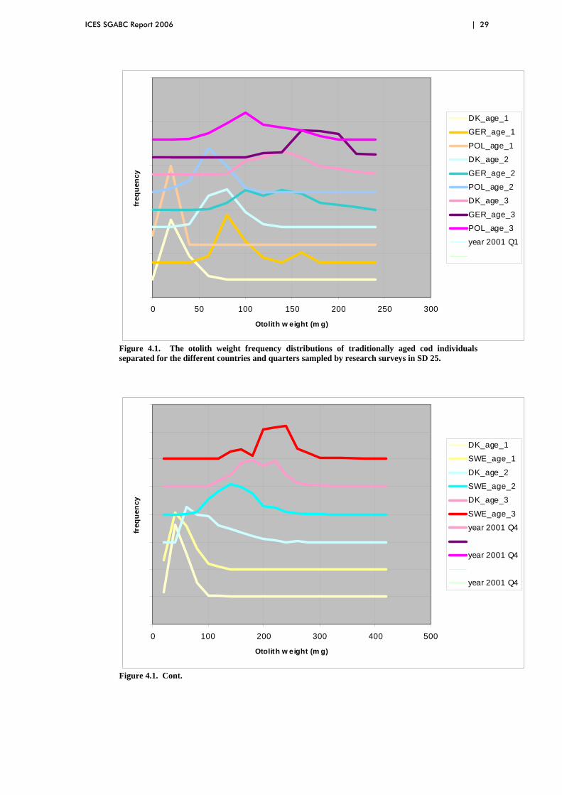
ICES SGABC Report 2006 | 29
Figure 4.1. The otolith weight frequency distributions of traditionally aged cod individuals separated for the different countries and quarters sampled by research surveys in SD 25.
Figure 4.1. Cont.
0 50 100 150 200 250 300
Otolith w eight (m g)
freq
uenc
y
DK_age_1
GER_age_1
POL_age_1
DK_age_2
GER_age_2
POL_age_2
DK_age_3
GER_age_3
POL_age_3
year 2001 Q1
0 100 200 300 400 500
Otolith w eight (m g)
freq
uenc
y
DK_age_1
SWE_age_1
DK_age_2
SWE_age_2
DK_age_3
SWE_age_3
year 2001 Q4
year 2001 Q4
year 2001 Q4

30 | ICES SGABC Report 2006
Figure 4.1. Cont.
Figure 4.1. Cont.
0 50 100 150 200 250 300
Otolith w eight (m g)
freq
uenc
yGER_age_1
POL_age_1
GER_age_2
POL_age_2
GER_age_3
POL_age_3
year 2002 Q1
0 100 200 300 400
Otolith w eight (m g)
freq
uenc
y
DK_age_1
POL_age_1
DK_age_2
POL_age_2
DK_age_3
POL_age_3
year 2002 Q4

ICES SGABC Report 2006 | 31
Figure 4.1. Cont.
Figure 4.1. Cont.
0 100 200 300 400 500
Otolith w eight (m g)
freq
uenc
yGER_age_1
POL_age_1
SWE_age_1
GER_age_2
POL_age_2SWE_age_2
GER_age_3
POL_age_3
SWE_age_3
year 2003 Q1
0 100 200 300 400
Otolith w eight (m g)
freq
uenc
y
DK_age_1
POL_age_1
SWE_age_1
DK_age_2
POL_age_2SWE_age_2
DK_age_3
POL_age_3
SWE_age_3
year 2003 Q4
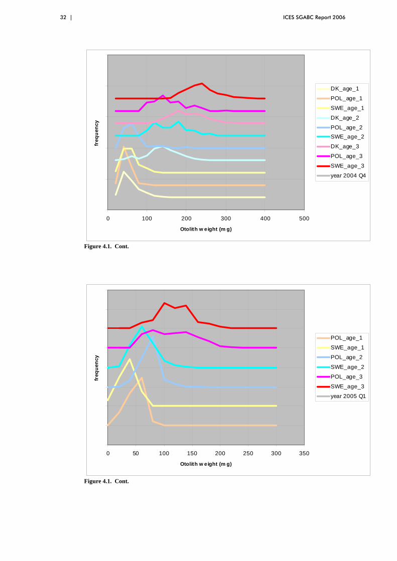
32 | ICES SGABC Report 2006
Figure 4.1. Cont.
Figure 4.1. Cont.
0 50 100 150 200 250 300 350
Otolith w eight (m g)
freq
uenc
y
POL_age_1
SWE_age_1
POL_age_2
SWE_age_2
POL_age_3
SWE_age_3
year 2005 Q1
0 100 200 300 400 500
Otolith w eight (m g)
freq
uenc
yDK_age_1
POL_age_1
SWE_age_1
DK_age_2
POL_age_2SWE_age_2
DK_age_3
POL_age_3
SWE_age_3
year 2004 Q4

ICES SGABC Report 2006 | 33
Figure 4.2.a. Otolith weight distribution in Q1 for the different countries.
Figure 4.2.b. Otolith weight distribution in Q4 for the different countries.
0 40 80 120
160
200
240
280
320
360
400
Otolith w eight (m g)
freq
uenc
y
DK_year_2001GER_year_2001POL_year_2001
0 40 80 120
160
200
240
280
320
360
400
Otolith weight (mg)
freq
uenc
y
GER_year_2002POL_year_2002
0 40 80 120
160
200
240
280
320
360
400
Otolith weight (mg)
freq
uenc
y
GER_year_2003POL_year_2003SWE_year_2003
0 40 80 120
160
200
240
280
320
360
400
Otolith w eight (m g)
freq
uenc
y
DK_year_2001SWE_year_2001
0 40 80 120
160
200
240
280
320
360
400
Otolith weight (mg)
freq
uenc
y
DK_year_2002POL_year_2002

34 | ICES SGABC Report 2006
Figure 5.1. The RELATIVE bias by modal age as estimated by all age readers combined.
Figure 5.2. Per cent agreement by modal age in the exchange set. It appears to be less difficult to reach a higher agreement on the age of the somewhat older individuals
-0.80
-0.60
-0.40
-0.20
0.00
0.20
0.40
0.60
0.80
0 1 2 3 4 5
% agreement by modal age
% agreement = 50.2054+3.3524*x; 0.95 Conf.Int.
0 1 2 3 4 5 6 7
MODAL AGE
30
40
50
60
70
80
90
100
110
% a
gree
men
t
MODAL AGE:% agreement: r = 0.1689, p = 0.0004
% agreement by modal age
% agreement = 50.2054+3.3524*x; 0.95 Conf.Int.
0 1 2 3 4 5 6 7
MODAL AGE
30
40
50
60
70
80
90
100
110
% a
gree
men
t
MODAL AGE:% agreement: r = 0.1689, p = 0.0004

ICES SGABC Report 2006 | 35
Figure 5.3. Current effect of reader on O1 (anova):F(9, 430)=10.338, p=.00000. Vertical bars denote 0.95 confidence intervals.
Figure 5.4. Variation in the median distance to rings from the standardised centre of the otolith. The variation is shown as a cumulative distribution.
Exchange 04/05
1 2 3 4 5 6 7 8 9 10
READER
0.1
0.2
0.3
0.4
0.5
0.6
0.7
0.8
0.9
Ave
rage
O1
(milli
met
er)
Distances from centre to WR
0
0.1
0.2
0.3
0.4
0.5
0.6
0.7
0.8
0.9
1
0 50 100 150 200 250 300 350 400 450
Distance (pix)
Cum
.freq
Dist 1WRDist 2WRDist 3WRDist 4WRDist 5WRDist 6WR

36 | ICES SGABC Report 2006
Figure 5.5. Example from the image analysis of an otolith where readers diverged to a high degree in interpretation of annual structures. Otolith from cod caught in Subdivision 25, March 2004.
Figure 5.6. Percentage agreement in relation to modal age in calibration set 1 and 2. It appears to be less difficult to reach a higher agreement on the age of the somewhat younger individuals in both calibration sets.
25 125 225 325 425 525 625 725 825 925 1025 1125 1225 1325
1-52_11:6
2-52_11:6
3-52_11:5
4-52_11:4
5-52_11:6
6-52_11:0
First calibration exercise
% Agreement = 85.4902-7.7648*x
0 1 2 3 4 5 6 7 8 9
Modal Age
30
40
50
60
70
80
90
100
110
% A
gree
men
t
Modal Age:% Agreement: r2 = 0.4208; r = -0.6487, p = 00.0000; y = 85.4902 - 7.7648*x Second calibration exercise
% Agreement = 78.0275-5.4493*x
0 1 2 3 4 5 6 7 8 9
Modal Age
30
40
50
60
70
80
90
100
110
% A
gree
men
t
Modal Age:% Agreement: r2 = 0.1949; r = -0.4415, p = 0.0000; y = 78.0275 - 5.4493*x

ICES SGABC Report 2006 | 37
Figure 5.7. Analysis of the effect of modal age on O1. In both calibration exercises the defined average O1 was significantly smaller in the younger individuals. Note the different scale on both X and Y axis.
Figure 5.8. Relationship between the standard deviation of O1 and % agreement.
Calibration 1: Closed diamonds, solid trendline (y=-0.0076x + 1.1016 R2 = 0.5959). Calibration 2: Open diamonds, broken trendline (y= -0.0086x + 0.9634 R2 = 0.8033)
First calibration exerciseCurrent effect of modal age on O1 (ANOVA):
F(5, 200)=2.5082, p=.03147Vertical bars denote 0.95 confidence intervals
1 2 3 4 5 8
Modal Age
0.8
1.0
1.2
1.4
1.6
1.8
2.0
2.2
2.4
2.6
2.8
O1
mm
Second calibration exerciseCurrent effect of modal age on O1 (ANOVA):
F(4, 214)=2.6637, p=.03355Vertical bars denote 0.95 confidence intervals
1 2 3 4 5
Modal Age
0.6
0.7
0.8
0.9
1.0
1.1
1.2
1.3
1.4
1.5
1.6
O1
(milli
met
er)
0
0.1
0.2
0.3
0.4
0.5
0.6
0.7
0.8
0.9
0 20 40 60 80 100 120
% Agreement
Stan
dard
dev
iatio
n of
O1

38 | ICES SGABC Report 2006
Figure 5.9. The change in standard deviation between calibration 1 and 2.
Mean calibration 1: 0.568 Mean calibration 2: 0.389 t-value = 1.910, p = 0.07 (n.s.)
Box & Whisker Plot of the standard deviation of O1 in the two reading calibrations
Mean Mean±SE Mean±1.96*SE
stdev calib1 stdev calib20.25
0.30
0.35
0.40
0.45
0.50
0.55
0.60
0.65
0.70
0.75
Sta
ndar
d de
viat
ion
on O
1

ICES SGABC Report 2006 | 39
Figure 5.10. An example of an otolith for which achieving a common O1 is difficult. A, B and C notes various interpretations of O1.
Figure 5.11. Distribution of agreed O1 in the exchange 04/05 and the recent discussion in the age reader subgroup in Gdynia, May 2006.
Agreed O1 exchange04/05: N = 7, Mean = 1.1567, StdDv = 0.2167, Max = 1.5036, Min = 0.8505.
Agreed O1 discussion06: N = 14, Mean = 2.5957, StdDv = 0.709, Max = 4.06, Min = 1.67
Distribution of agreed O1 in exchange and O1 discussion
Agreed O1exchange04/05Agreed O1 discussion060.5 1.0 1.5 2.0 2.5 3.0 3.5 4.0 4.5
O1 (millimeter)
0
1
2
3
4
5
6
No
of o
bs

40 | ICES SGABC Report 2006
O1 as agreed in discussion during SGABC, May 2006Current effect of month on O1: F(4, 9)=4.6629, p=.02584
Vertical bars denote 0.95 confidence intervals
2 3 4 9 11
Month (3-11 in 2005; 2 in 2006)
0.5
1.0
1.5
2.0
2.5
3.0
3.5
4.0
4.5
5.0O
1 (m
illim
eter
)
Figure 5.12. Seasonal development of O1 in the otoliths agreed by the group during SGABC, Gdynia, May 2006.

ICES SGABC Report 2006 | 41
Annex 1: Agenda for the SGABC meeting in Gdynia, 16–19 May 2006
MAIN AGENDA:
Tuesday 16th May, meeting starts at 10.00
1. Morning session
1.1. Welcome and housekeeping organisation.
1.2. Discussions on agenda and work schedule
1.3. Presentations
1.4. Organisation of tasks
1.5. Agreement on report outline
2. Afternoon session
2.1. Split into age-reading and modelling subgroups
2.2. Analysis and text production
Wendnesday 17th May, meeting starts at 09.00
3. Analysis and text production
Thursday 18th May, meeting starts at 09.00
4. Morning session
4.1. Review of work progress incl. suggested recommendations
4.2. Analysis and text production
5. Afternoon session
5.1. Preliminary results on age reader calibration and agreements
5.2. Preliminary results on model development
5.3. Discussions and recommendations on post-meeting work
5.4. Analysis and text production
Friday 19th May, meeting starts at 09.00
6. Text review
7. Recommendations

42 | ICES SGABC Report 2006
Age Reader Subgroup Agenda:
Tuesday May 16th
1 ) Introduction to the subgroup and the agenda 2 ) The recent analysis of previous exchanges and the size of the otolith at O1. 3 ) First reading calibration exercise. ‘Ordinary’ approach, using stereomicroscopes
and computers for the pointing of age structures 4 ) Discussion of O1 in the most recent collected otoliths. The aim is to reach an
agreement on an average O1 by area and season, acknowledging both year-to-year variation and growth effects.
Wednesday May 17th
5 ) First rough and dirty results from the calibration yesterday – do we still disagree on the same structures?
6 ) Second reading calibration exercise. This time using all metric possibilities available in addition to the ‘ordinary’ approach
7 ) Back-calculation of lengths – can we use back-calculated length-at-age as a guideline if the age structures are too difficult to identify?
8 ) Group discussion of a common set of ‘rules-of-thumb’ for age determination of Baltic cod. Not necessarily a long document, more in the line of a couple of pages with guidelines for new and experienced readers, that may guide all readers into a more common interpretation of age structures regardless the origin of the cod.

ICES SGABC Report 2006 | 43
Annex 2: List of participants
NAME ADDRESS PHONE/FAX EMAIL
Ann-Sofie Ågren National Board of Fisheries Institute of Marine Research Utövägen 5 371 37 Karlskrona Sweden
+46-455362856 [email protected]
Egidijus Bacevicius Fishery Research Laboratory PO Box 108 LT 91001 KLAIPEDA Latvia
+370-46-391122 [email protected] [email protected]
Tatjana Baranova LFRA Daugavgrivas Street 8 LV-1048 Riga Latvia
+37-17610766 [email protected]
Max Cardinale National Board of Fisheries Institute of Marine Research Box 4 SE-453 21 Lysekil Sweden
+46-52318750 [email protected]
Lotte Worsøe Clausen
DIFRES Charlottenlund Slot DK-2920 Charlottenlund Denmark
+45-33963364 [email protected]
Elena Fedotova Fishery Research Laboratory PO Box 108 LT 91001 Klaipeda Latvia
+370-46391122 [email protected] [email protected]
Edyta Gosz Sea Fisheries Institiute Kollataja 1 81-332 Gdynia Poland
+48-587356211 [email protected]
Igor Karpushevskiy AtlantNIRO 5, Dmitry Donskogo Street 236000 Kaliningrad, Russia
+0074012225560 [email protected]
Svend Erik Levinsky DIFRES Charlottenlund Slot DK-2920 Charlottenlund Denmark
+4533963444 [email protected]
Johan Modin (Chair)
Swedish Board of Fisheries P.O. Box 109 SE-74071 Öregrund, Sweden
+46-173-46463 [email protected]
Henrik Mosegaard DIFRES Charlottenlund Slot DK-2920 Charlottenlund Denmark
+45-33963461 [email protected]

44 | ICES SGABC Report 2006
Tomasz Nermer Sea Fisheries Institiute Kollataja 1 81-332 Gdynia Poland
+48-587356211 [email protected]
Krzysztof Radtke Sea Fisheries Institute Kollataja 1 81-332 Gdynia Poland
+48-587356269 [email protected]
Rajlie Sjóberg National Board of Fisheries Institute of Marine Research Box 4 SE-453 21 Lysekil Sweden
+46-52318726 [email protected]
Britta Stepputis Federal Research Centre for Fisheries Institute for Baltic Sea Fisheries Alter Hafen Süd 2 D-18069 Rostock Germany
+49-3818116151 [email protected]
Andrés Velasco Institute for Baltic Sea Fisheries Rostock Germany
+49-3818116123 [email protected]
Marianna Wolfram Federal Research Centre for Fisheries Institute for Baltic Sea Fisheries Alter Hafen Süd 2 D-18069 Rostock Germany
+49-3818116150 [email protected]
Dace Zilniece LFRA Daugavgrivas Street 8 LV-1048 Riga Latvia
+37-17610766 [email protected]

ICES SGABC Report 2006 | 45
Annex 3: Recommendation buzzlist
RECOMMENDATION ACTION 1. Application for research programme on otolith growth DFU, General, Baltic Committee 2. Establishment of an “age” coordinator WGBFAS 3. Compilation of otolith weight data in other cod stocks ICES assessment WGs 4. Calibration and validation of otolith growth models General, Baltic Committee 5. Initiation of mark and recapture programs General, Baltic Committee 6. Sampling and analysis of very young cod General, Baltic Committee 6. Studies to infer known-age Baltic cod from other methods General, Baltic Committee 7. Coordination of otolith weight database DFU, WGBFAS 8. Otolith database storage ICES DATRAS, FISHFRAME 9. Use of otolith biometrics in other stocks General, Baltic Committee 10. Use of the SGABC image calibration tool General, Baltic Committee 11. An age calibration exercise DFU, WGBFAS