REPORT OF THE COMMITTEE - sdnbd.org · REPORT OF THE COMMITTEE ... fractile) to 65.70 Tcf ......

$: REPORT OF THE COMMITTEE - sdnbd.org · REPORT OF THE COMMITTEE ... fractile) to 65.70 Tcf ... within 200 meter water depth and the resource forecast was made for a period of 30$
REPORT OF THE COMMITTEE FOR

GAS DEMAND PROJECTIONS AND DETERMINATION OF RECOVERABLE RESERVE & GAS RESOURCE POTENTIAL

IN BANGLADESH

PREPARED FOR

MINISTRY OF ENERGY AND MINERAL RESOURCES GOVERNMENT OF THE PEOPLE’S REPUBLIC OF BANGLADESH

DHAKA; JUNE 2002

PREFACE Government of the People’s Republic of Bangladesh intends to formulate some policies regarding energy issues in general and natural gas resources in particular. As such the Ministry of Energy and Mineral Resources of the Government of Bangladesh constituted two national Committees – one to report on the resource potential and recoverable reserve of natural gas in Bangladesh and the demand scenario for future years; another national Committee has been entrusted to evaluate and suggest the options available to the Government for better utilization of its natural gas resource for the benefit of the country. Constitution of both these national Committees has the approval of the Head of the Government i.e. the Prime Minister of Bangladesh. The Terms of Reference of the Committee were:

a. assessment of the resource potential and the recoverable reserve by updating proven, probable and possible natural gas reserve discovered in the country.

b. projection of future demand for natural gas in the country in different

scenarios. Notification of the Ministry of Energy and Mineral Resources of the Government of Bangladesh dated 26 December, 2001 has been attached to this report as Appendix-A. The notification has been published in the Bangladesh Gazette Page No. 10949 dated December 26, 2001.

The Committee consists of the following: Prof. Nooruddin Ahmed Ph.D. - Chairman Vice-Chancellor, BUET Prof. Ijaz Hossain Ph.D. - Member Chemical Engineering Department, BUET Prof. M. Nurul Islam Ph.D. - Member Institute of Appropriate Technology, BUET Prof. M. Tamim Ph.D. - Member Petroleum and Mineral Resources Engineering Department, BUET Prof. Edmond Gomes Ph.D. - Member Petroleum and Mineral Resources Engineering Department, BUET

i

Prof. A.S.M. Woobaidullah Ph.D. Chairman, Department of Geology - Member

University of Dhaka Prof. Khalilur Rahman Chowdhury Ph.D. - Member Department of Geology Jahangirnagar University, Savar M. Nazrul Islam

Director General - Member Geological Survey of Bangladesh M. Ismail Ph.D. -Member-Secretary Director (Operations) Petrobangla The first meeting of the Committee was held on January 12, 2002. Subsequently, seventeen (17) meetings were held, some lasting as long as four (4) hours. Initially, a time frame of thirty (30) days was given. Later, because of the complexity of the nature of the work it was extended to March 31, 2002. The work of the Committee was delayed by about a month since the Chairman and some Members had to go abroad for personal/official reasons. The Members of the Committee have worked hard to discharge the responsibility given to them by the Government. They are holding full-time positions in Universities/Petrobangla/GSB. All the work will be worthy of it if and when the findings of the Committee will be used by the concerned authorities in taking appropriate decisions. The Chairman would like to take this opportunity to thank the Members for their hard work, understanding, cooperation and support given during the deliberations and the write-up. The Committee would like to take this opportunity to thank the staff of the Vice-Chancellor’s office for their tireless effort in preparing the report.

ii

EXECUTIVE SUMMARY

There are considerable uncertainties in the estimation of energy/gas demand, gas

reserves and gas resources based on available data. Best possible judgement has been

made by the Committee.

(a) Energy Demand Projection

Energy demand projection for a developing country is an extremely difficult thing to

perform. This is because economic growth, which is the main driver for energy

growth, is very difficult to predict. The methodology based on energy intensity of the

economy was employed. Several scenarios were used to get an understanding of the

energy requirement for a level of economic performance. The natural gas requirement

from 2000 to 2050 has been summarized as follows:

If the economic performance is on the low side (3% GDP growth rate), the total gas

requirement will be between 40 and 44 Tcf.

If economic performance continues according to the historical trend (Business-as-

usual; 4.55% GDP growth rate), gas requirement will be between 64 and 69 Tcf.

If performance is on the moderately high side (6% GDP growth rate), gas


If performance is on the high side (7% GDP growth rate), gas requirement will be

between 141 and 152 Tcf.

(b) Recoverable Reserve

Reserve estimation is a dynamic process and therefore, the estimated reserves need to

be updated with additional pressure/production data and with new information of the

appraisal/development activities. All estimated reserve figures are associated with

certain degrees of uncertainties. Exact reserve of the country will be known for

sure on the day when all the gas fields will be depleted. But for optimum utilization

of this valuable national resource and for long term energy planning, efforts should be

made to find the best estimates with latest available information of the gas fields.

iii

In estimating the reserve, all published studies/reports available to the Committee have

been reviewed and carefully scrutinized. Industry standard procedure and definitions

have been followed in classifying reserves into proved (P1), probable (P2), possible

(P3) categories and in estimating their values. Mostly published reports/studies have

been considered and up to date data and information have been used in updating the

reserve. The important factors considered in judging the previous studies/reports

include: estimation methodology, timing of the study, data and information used and

their quality, and reservoir model and drive mechanism assumed.

After carefully reviewing the available studies/reports and analyzing the latest

information of the reservoir, the Committee concludes that as of April 2002, the

proved + probable (2P) reserve of the country lies between 12.04 Tcf and 15.55 Tcf

for 22 gas fields. The possible (P3) gas in place (GIIP) was estimated to be in the rage

of 4.14 Tcf to 11.84 Tcf. To reduce uncertainties in the reserve estimates, the

Committee recommends developing all gas fields to their full extent and update

reserves on a regular basis.

(c) Gas Resource Potential

The undiscovered resource assessment is basically a combination of hypothetical and

speculative numbers with little or no economic considerations. As such, these numbers

may only be used for petroleum exploration purposes, and not for petroleum

exploitation planning.

After thorough examination of all available estimates of undiscovered resources

assessment, this Committee feels that the 2001 USGS-Petrobangla Gas Resources

Assessment be considered to reflect the country’s undiscovered gas resources. The

study estimated a total undiscovered gas resource potential ranging from 8.43 Tcf (95

fractile) to 65.70 Tcf (05 fractile), with a Monte Carlo Simulation mean of 32.12 Tcf.

The minimum field size considered in the study was 42 Bcf, offshore prospectivity

within 200 meter water depth and the resource forecast was made for a period of 30

years.

iv

(d) Concluding Remarks

According to terms of reference the Committee has estimated three sets of data

required to take decisions on future use of natural gas. These data are natural gas

demand up to 2050, net recoverable reserves of natural gas from discovered fields and

natural gas resources in undiscovered areas. Natural gas demand projection period is

considered from year 2000 to 2050. In two years from 2000 to 2002, an estimated 0.7

Tcf gas has already been consumed. The summary of information is presented below:

(i) Natural gas demand up to 2020: 9.9 Tcf (10.6-0.7) to 17.4 Tcf (18.1-0.7)

(ii) Natural gas demand up to 2050: 39.3 Tcf (40.0-0.7) to 151.3 Tcf (152.0-0.7)

(iii) Net recoverable reserves of natural gas (as on May 2002) lies in a range of

12.04 Tcf to 15.55 Tcf

(iv) Natural gas resources in undiscovered areas: 8.4 Tcf (95F) to 65.7 Tcf (05F)

with a Monte Carlo Simulation mean of 32.0 Tcf

It may be mentioned here that there are some uncertainties in the estimated values of

the above mentioned figures. There is no way to estimate these accurately and

correctly. Therefore, these figures should be used with proper care and understanding.

v

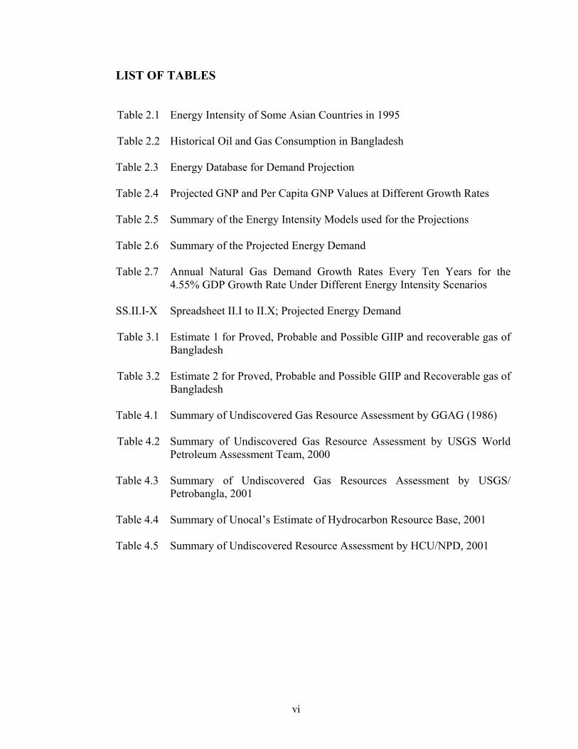
LIST OF TABLES Table 2.1 Energy Intensity of Some Asian Countries in 1995 Table 2.2 Historical Oil and Gas Consumption in Bangladesh Table 2.3 Energy Database for Demand Projection Table 2.4 Projected GNP and Per Capita GNP Values at Different Growth Rates Table 2.5 Summary of the Energy Intensity Models used for the Projections Table 2.6 Summary of the Projected Energy Demand Table 2.7 Annual Natural Gas Demand Growth Rates Every Ten Years for the

4.55% GDP Growth Rate Under Different Energy Intensity Scenarios SS.II.I-X Spreadsheet II.I to II.X; Projected Energy Demand Table 3.1 Estimate 1 for Proved, Probable and Possible GIIP and recoverable gas of

Bangladesh Table 3.2 Estimate 2 for Proved, Probable and Possible GIIP and Recoverable gas of

Bangladesh Table 4.1 Summary of Undiscovered Gas Resource Assessment by GGAG (1986) Table 4.2 Summary of Undiscovered Gas Resource Assessment by USGS World

Petroleum Assessment Team, 2000 Table 4.3 Summary of Undiscovered Gas Resources Assessment by USGS/

Petrobangla, 2001 Table 4.4 Summary of Unocal’s Estimate of Hydrocarbon Resource Base, 2001 Table 4.5 Summary of Undiscovered Resource Assessment by HCU/NPD, 2001

vi

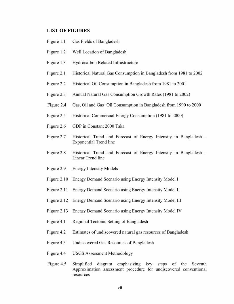
LIST OF FIGURES Figure 1.1 Gas Fields of Bangladesh Figure 1.2 Well Location of Bangladesh Figure 1.3 Hydrocarbon Related Infrastructure Figure 2.1 Historical Natural Gas Consumption in Bangladesh from 1981 to 2002 Figure 2.2 Historical Oil Consumption in Bangladesh from 1981 to 2001 Figure 2.3 Annual Natural Gas Consumption Growth Rates (1981 to 2002) Figure 2.4 Gas, Oil and Gas+Oil Consumption in Bangladesh from 1990 to 2000 Figure 2.5 Historical Commercial Energy Consumption (1981 to 2000) Figure 2.6 GDP in Constant 2000 Taka Figure 2.7 Historical Trend and Forecast of Energy Intensity in Bangladesh –

Exponential Trend line Figure 2.8 Historical Trend and Forecast of Energy Intensity in Bangladesh –

Linear Trend line Figure 2.9 Energy Intensity Models Figure 2.10 Energy Demand Scenario using Energy Intensity Model I Figure 2.11 Energy Demand Scenario using Energy Intensity Model II Figure 2.12 Energy Demand Scenario using Energy Intensity Model III Figure 2.13 Energy Demand Scenario using Energy Intensity Model IV

Figure 4.1 Regional Tectonic Setting of Bangladesh Figure 4.2 Estimates of undiscovered natural gas resources of Bangladesh Figure 4.3 Undiscovered Gas Resources of Bangladesh Figure 4.4 USGS Assessment Methodology Figure 4.5 Simplified diagram emphasizing key steps of the Seventh

Approximation assessment procedure for undiscovered conventional resources

vii

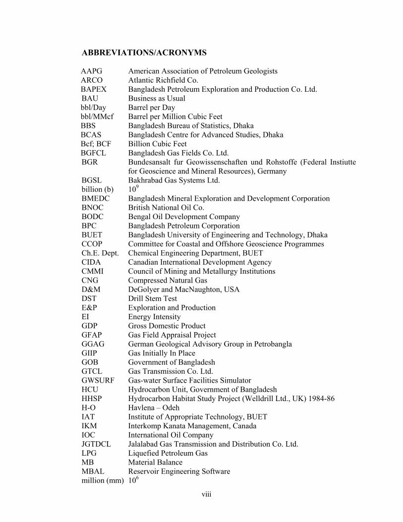
ABBREVIATIONS/ACRONYMS AAPG American Association of Petroleum Geologists ARCO Atlantic Richfield Co. BAPEX Bangladesh Petroleum Exploration and Production Co. Ltd. BAU Business as Usual bbl/Day Barrel per Day bbl/MMcf Barrel per Million Cubic Feet BBS Bangladesh Bureau of Statistics, Dhaka BCAS Bangladesh Centre for Advanced Studies, Dhaka Bcf; BCF Billion Cubic Feet BGFCL Bangladesh Gas Fields Co. Ltd. BGR Bundesansalt fur Geowissenschaften und Rohstoffe (Federal Instiutte

for Geoscience and Mineral Resources), Germany BGSL Bakhrabad Gas Systems Ltd. billion (b) 109 BMEDC Bangladesh Mineral Exploration and Development Corporation BNOC British National Oil Co. BODC Bengal Oil Development Company BPC Bangladesh Petroleum Corporation BUET Bangladesh University of Engineering and Technology, Dhaka CCOP Committee for Coastal and Offshore Geoscience Programmes Ch.E. Dept. Chemical Engineering Department, BUET CIDA Canadian International Development Agency CMMI Council of Mining and Metallurgy Institutions CNG Compressed Natural Gas D&M DeGolyer and MacNaughton, USA DST Drill Stem Test E&P Exploration and Production EI Energy Intensity GDP Gross Domestic Product GFAP Gas Field Appraisal Project GGAG German Geological Advisory Group in Petrobangla GIIP Gas Initially In Place GOB Government of Bangladesh GTCL Gas Transmission Co. Ltd. GWSURF Gas-water Surface Facilities Simulator HCU Hydrocarbon Unit, Government of Bangladesh HHSP Hydrocarbon Habitat Study Project (Welldrill Ltd., UK) 1984-86 H-O Havlena – Odeh IAT Institute of Appropriate Technology, BUET IKM Interkomp Kanata Management, Canada IOC International Oil Company JGTDCL Jalalabad Gas Transmission and Distribution Co. Ltd. LPG Liquefied Petroleum Gas MB Material Balance MBAL Reservoir Engineering Software million (mm) 106

viii

mmbbl Million Barrel MMcf Million Cubic Feet mtoe million ton of oil equivalent NORAD Norwegian Agency for Development NPD Norwegian Petroleum Directorate OBL Occidental of Bangladesh Limited ODA Overseas Development Agency, UK OECF Overseas Economic Cooperation Fund, Japan OGDVC Oil and Gas Development Corporation ONGC Oil and Natural Gas Corporation OXY Occidental Oil, USA Petrobangla Bangladesh Oil, Gas and Mineral Corporation (BOGMC) PMRE Petroleum and Mineral Resources Engineering Department, BUET POL Petrol, Oil, Lubricant PPL Pakistan Petroleum Ltd. PSC Production Sharing Contract PSOC Pakistan Shell Oil Company RPGCL Rupantarita Prakritik Gas Co. Ltd. SAPS Special Assistance for Project Sustainability SBED Shell Bangladesh Exploration and Development B.V. SGFL Sylhet Gas Fields Ltd. SPE Society of Petroleum Engineers, USA SVOC Standard Vacuum Oil Co., USA Tcf; TCF Trillion Cubic Feet TD Total Depth TGTDCL Titas Gas Transmission and Distribution Co. Ltd. thousand (m) 103 TOC Total Organic Content toe Ton Oil Equivalent trillion (t) 1012 UMC United Meridian Corporation UN/ECE United Nations/Economic Commission for Europe UNOCAL Unocal Bangladesh Ltd WDR World Development Report WESGAS Paschimanchal Gas Co. Ltd. WPC World Petroleum Congress

ix

REPORTS AND PAPERS MADE AVAILABLE TO THE COMMITTEE • Report on the Hydrocarbon Habitat Study (HHS) (1984-86)

Volumes I and II, December, 1986 (Welldrill Limited, UK)

• Review of Recoverable Gas Reserves in Bangladesh for BOGMC

Welldrill Limited, UK, November, 1991 • Gas Field Appraisal Project Management Report, Bangladesh

Intercomp-Kanata Management Ltd. (IKM), April, 1992 (Prepared for CIDA and BOGMC)

• Natural Gas Demand and Supply Forecast: Bangladesh

FY 2001 to 2050 M. Abdul Aziz Khan, Petrobangla, March, 2001

• Bangladesh 2020, A Long-Run Perspective Study

The World Bank and BCAS, September, 1998 Published for the World Bank The University Press Limited, Dhaka • National Energy Policy

Ministry of Energy and Mineral Resources, GOB Dhaka, September, 1995

• Quader, AKMA and Edmond Gomes – An Exploratory Review of Bangladesh Gas Sector: Latest Evidence and Areas of Further Research

Centre for Policy Dialogue, January 24, 2002 • Energy Sectoral Plan and Vision Statement

Petrobangla, April, 2001 • Reserve Estimation Report of Shahbazpur

BAPEX, February, 1996 • Study of Habiganj upper Sands

Hydrocarbon Resources for Enhanced Reservoir (Asset) Management Reservoir Study Cell, Petrobangla & Beicip-Franlab Consultants Interim Report, July, 2000

• Study of Bakhrabad Field Hydrocarbon Resources for Enhanced Reservoir (Asset) Management

Reservoir Study Cell, Petrobangla & Beicip-Franlab Consultants Interim Report, November, 2000

x

• Report on Reserves of the Bibiyana Field

DeGolyer & MacNaughton, USA January 31, 2000

• Certificate of Gas Reserves (Bibiyana Field)

DeGolyer & MacNaughton, USA August 1, 2000

• U.S. Geological Survey – Petrobangla Cooperative Assessment of Undiscovered Natural Gas Resources of Bangladesh

January 2001 • Strategic Gas Utilization Study for the People’s Republic of Bangladesh

Final Report, S.H. Lucas & Associates, USA January 22, 2002

• Bangladesh Petroleum Potential and Resource Assessment 2001

Hydrocarbon Unit, MEMR, GOB and Norweigian Petroleum Directorate March, 2002

• Estimation of Gas In Place of Bangladesh Using Flowing Material Balance Method

M. Bashirul Haq & Edmond Gomes PMRE Dept., BUET, Dhaka 4th Interntional Conference on Mechanical Engineering (ICME), December 26-28, 2001; Dhaka, Bangladesh, Section VII, pp. 83-88.

• Natural Gas Demand in Bangladesh to 2020

Multi-client Study Wood MacKenzie a Division of Deutsche Bank AG.; June, 2001

• Sangu Field Reservoir Performance and Reserves

Update June 2000 Shell Bangladesh Exploration and Development B.V.

• Petroleum Exploration Opportunities in Bangladesh

Petrobangla, February, 2000 • Energy Scenario and Policy in Bangladesh

Keynote paper, M. Nurul Islam, Institute of Appropriate Technology, BUET, Dhaka 4th Interntional Conference on Mechanical Engineering (ICME), December 26-28, 2001; Dhaka, Bangladesh

xi

• Energy Security in Bangladesh

Prof. M. Nurul Islam, Paper presented in the Dhaka Meet on Sustainable Development in Bangladesh; Achievements, Opportunities, and Challenges at Rio+10; Organized by Bangladesh Unnayan Parishad (BUP), Dhaka, 15-18 March, 2002.

xii

Page No.

PREFACE i

EXECUTIVE SUMMARY iii

LIST OF CONTENTS

LIST OF TABLES vi

LIST OF FIGURES vii

ABBREVIATIONS/ACRONYMS viii

REPORTS AND PAPERS MADE AVAILABLE TO THE COMMITTEE x

1. INTRODUCTION 1

2. ENERGY DEMAND PROJECTION UPTO 2050 8 2.1 Introduction 9 2.2 Energy Intensity 10 2.3 Oil and Gas Consumption in Bangladesh 12

2.4 Commercial Energy Demand Projection 18

2.5 Conclusions 35 2.6 References 39 3. ASSESSMENT OF RECOVERABLE GAS RESERVE 50 3.1 Introduction 51 3.2 Review of Past Reports 51 3.3 Methodology of Reserve Estimates 54 3.4 Reserve Classification 56 3.5 Recovery Calculation 58 3.6 Estimation of Reserves 59 3.7 Conclusions 63 3.8 Recommendations 64 3.9 References 64

xiii

4. GAS RESOURCE ASSESSMENT 66 4.1 Introduction 67 4.2 Regional Geological Setting and Tectonic Evolution 68 4.3 Petroleum System and Assessment Units 68 4.4 Assessment Methodology/Approaches 80 4.5 Summary of Undiscovered Resource Assessment 85 4.6 Observations and Comments 91 4.7 Conclusions 95 4.8 References 96

APPENDIX-A : Government Notifications regarding constitution of the Committee.

xiv

1. INTRODUCTION

1

1. INTRODUCTION

Natural gas is considered a very clean source of energy all around the world, more so

after the oil shock of the seventies and increasing environmental awareness about

burning coal. Natural gas as found in the gas fields of Bangladesh is 95% methane

(CH4) and is sulfur free. Because natural gas as found in Bangladesh contains mainly

C1 compound (CH4), this gas is not suitable as feedstock for petrochemicals. Absence

of sulfur compounds makes it sweet compared to sour gas as found in some other

countries. This also reduces/eliminates corrosion problems associated with raw sour

gas. Bangladesh being a small country, so far all the gas transmitted from the fields to

the power plants/fertilizer factories, commercial and domestic users has been without

the necessity of any booster compressor thus reducing cost of transmission. Gas

transmission through underground steel pipe line system is a standard fool proof

technology. With the availability of cathodic protection (CP) system for corrosion

prevention, underground and underwater pipe lines are not subject to soil and water

corrosion problems. Transmission of gas from one place to other is safe and reliable.

Natural gas is the most important indigenous energy source in Bangladesh. It is the

principal source of energy for power, industry, commercial and domestic sectors. It is

also the feedstock of all the urea fertilizer plants in the country. Urea has helped

Bangladesh attain self-sufficiency in rice – the major local food-crop. Recently, the

Government of Bangladesh has decided to use compressed natural gas (CNG) as a

substitute for gasoline (petrol) and diesel in the transport sector as has been done in

Italy, New Zealand and many other countries. This is being done to reduce the import

bill of liquid fuels viz. crude oil for the only oil refinery, gasoline and diesel.

Natural gas was first discovered in Bangladesh in 1955 at Haripur (Sylhet Gas Field).

Chhatak gas field was discovered in 1959. Subsequently, thus far 22 gas fields and one

small oil field have been discovered.

Bangladesh Oil, Gas and Mineral Corporation (BOGMC) popularly known as

Petrobangla, a fully state-owned Corporation and its subsidiary companies like

BAPEX, BGFCL, Titas Gas, etc. are responsible for exploration, production,

transmission, distribution and development of oil, gas and other mineral resources of

the country. Bangladesh Petroleum Corporation (BPC), another state owned 2

corporation is responsible for import of crude oil and other petroleum products,

refining, and marketing of liquid petroleum products including LPG. Only recently,

some private companies have been allowed to import, bottle and market LPG for

domestic consumption in areas where pipe line gas is not available.

BAPEX, a subsidiary organization of Petrobangla is involved with exploration work

with its limited financial resources. Some International Oil Companies (IOCs) are

involved in exploration and production of natural gas through Production Sharing

Contracts (PSC) with Petrobangla. Companies producing natural gas in Bangladesh

are:

• Bangladesh Gas Fields Company Ltd. (BGFCL) (operates Titas, Habiganj, Bakhrabad, Narsingdi, Meghna, Begumganj, Feni and Kamta gas fields)

• Sylhet Gas Fields Ltd. (SGFL) (operates Sylhet, Kailashtila, Rashidpur, Beanibazar and Chhatak gas fields)

• Bangladesh Petroleum Exploration and Production Company Ltd. (BAPEX) (operates Saldanadi, Fenchuganj and Shahbazpur gas fields)

• Shell Bangladesh Exploration and Development B.V (SHELL) (operates Sangu, Semutang and Kutubdia gas fields)

• UNOCAL Bangladesh Ltd. (UNOCAL) (UNOCAL is the successor company of Occidental, Bangladesh) (operates Jalalabad, Moulvibazar and Bibiyana gas fields)

Of these producing companies the first three are SOEs and the last two are IOCs

operating in Bangladesh under PSCs.

Figures 1.1, 1.2 and 1.3 depict different aspects of gas and oil sector of Bangladesh.

Quantification of energy source such as natural gas reserve is important for energy

sector planning and investments. But gas reserve estimation is not a simple matter. It

is rather complex and a dynamic process. Oil/Gas reserves are usually updated with

exploratory drilling, production and development activities. Laymen often get

confused with the use and misuse of the terms such as resource potential, gas initially

in place (GIIP) and gas reserve. Reserve figures are again categorized by proven (P1),

probable (P2) and possible (P3) reserves. Thus, one must be very clear about what one

is talking about while mentioning numerical figures quantifying gas wealth. All these 3

oints have been clearly discussed and enumerated in the following chapters of this

report.

Gas demand projection for a country for a definite time period is another sector which

is difficult because of assumptions involved in estimating such projections. Usually,

demand projections are made assuming different economic scenarios.

Because of the complexity, assumptions and uncertainties involved, different reputed

international consulting houses employed by Petrobangla or donor agencies have

come up with different figures at different times. In this report sincere efforts have

been made to forecast country’s gas demand, estimate gas reserves and resource

potential of the country objectively and professionally.

4

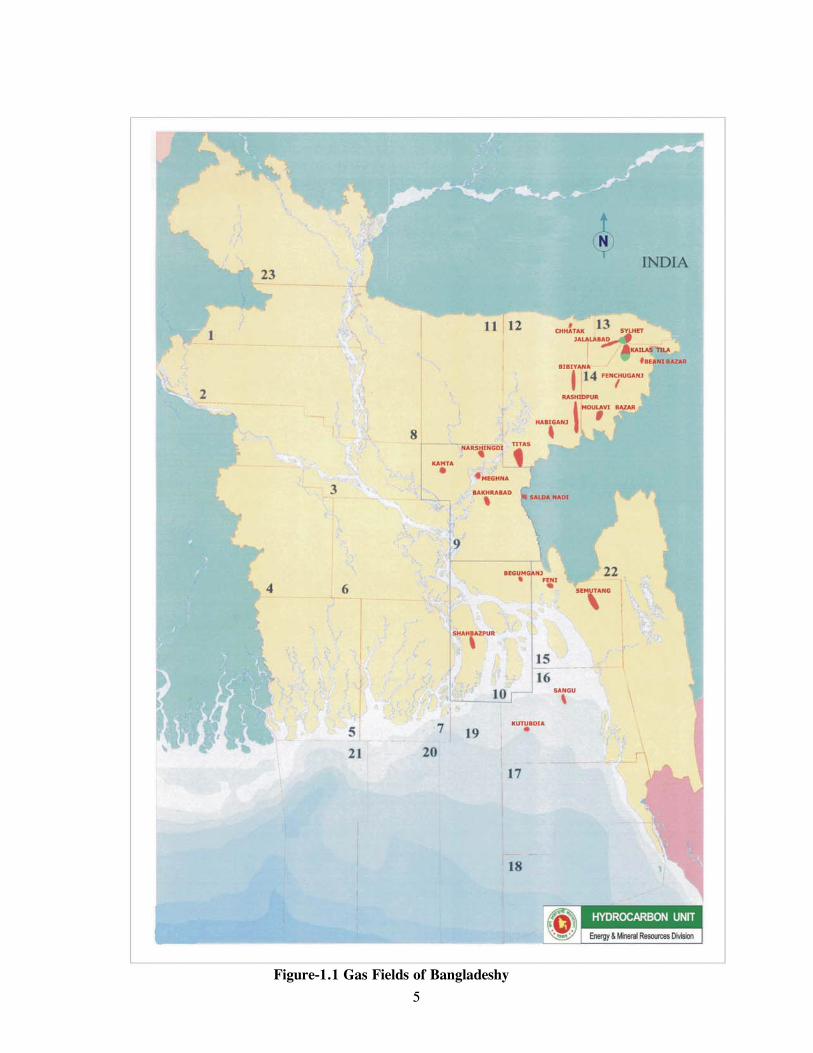
Figure-1.1 Gas Fields of Bangladeshy

5

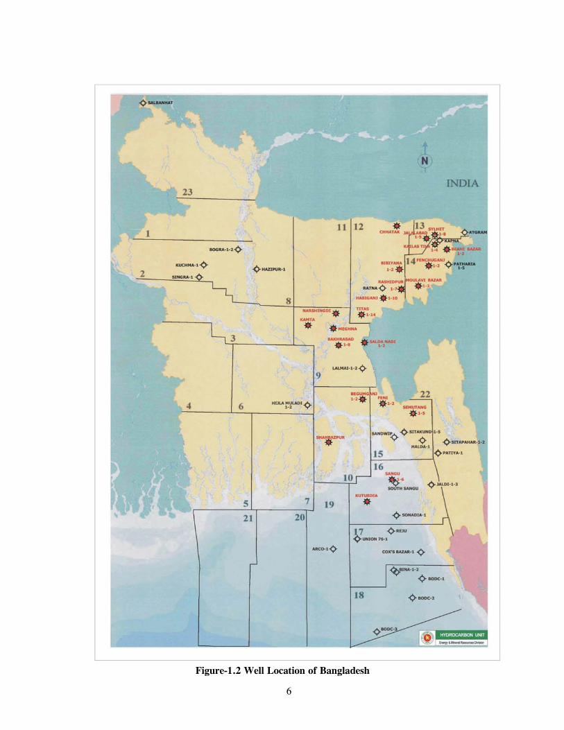
Figure-1.2 Well Location of Bangladesh

6

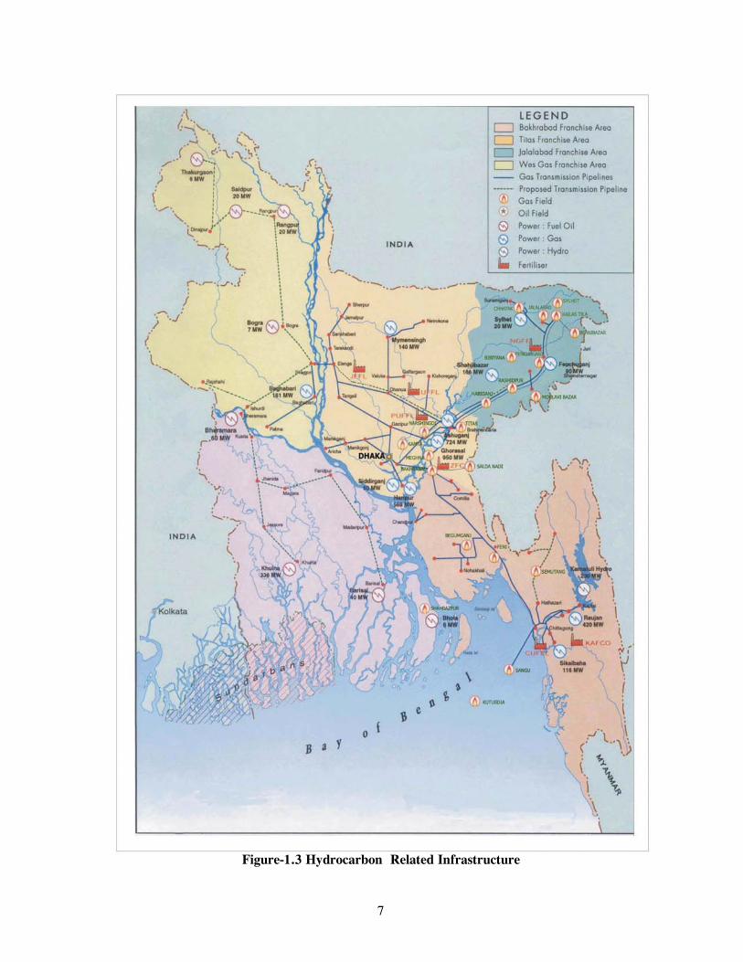
Figure-1.3 Hydrocarbon Related Infrastructure

7

2. ENERGY DEMAND PROJECTION UP TO 2050

8

2.1 Introduction

Energy demand projection for a developing country is an extremely difficult thing to

perform. This is because economic growth, which is the main driver for energy growth, is

very difficult to predict. It is axiomatic that if a developing country continues to achieve

economic growth energy demand will keep on rising. Apart from mature economies, a

decline in energy demand signals economic decline or recession. The best example of this

can be found in the East European countries. In these countries energy demand fell

dramatically with economic collapse experienced in the late eighties.

There are several different methodologies available for energy demand projection,

but the simplest two and hence most commonly used ones are

1. Projections based on the energy intensity of the economy (Top down approach)

2. Projections derived from disaggregated energy growth analysis (Bottom up

approach)

A disaggregated or sectoral type projection validated by a top down macroeconomic model

is the most desirable. Even for the simplest level of disaggregation, the exercise will be

laborious and time-consuming. Therefore, such a projection is outside the Committee’s

scope of work. The Committee has endeavored to provide an expert opinion on the probable

range of energy and gas requirements up to 2050 given different economic growth rates.

The task of projecting energy demand becomes that much more difficult when the horizon is

long. Thus energy demand projections beyond 25 to 30 years cannot be performed using

sectoral type analysis unless the sectoral growth pictures are known with reasonable

certainty. In a country like Bangladesh it is almost impossible to predict energy growth

based on purely sectoral analysis. In developing countries large growth potential cannot be

predicted for existing economic activities and new economic activities are difficult to

visualize. In addition, the detailed and involved nature of data collection and analysis of the

disaggregated demand projections precluded its use for this Committee’s work. In view of

the above, the methodology based on energy intensity of the economy had to be employed

9

by the Committee. Before presenting the Demand Projections, the energy intensity concept

is briefly described and an account of the historical consumption of gas and oil is provided.

2.2 Energy Intensity

The energy intensity (EI) is a very useful parameter to understand the energy

consumption in a country. EI is defined as

Commercial energy consumption (toe) GDP

To avoid very small numbers, the unit of EI can be expressed as kgoe/Taka. As is

clearly evident, EI gives the energy requirement per unit of GDP. If a projection of

GDP in constant Taka (the year for which EI was calculated) is available, it can be

multiplied by EI to get the energy requirement in the future. This conceptually

simple-to-understand methodology would have given a reliable energy demand

projection for different GDP growth rates had EI been constant. It is very difficult to

predict how EI will behave in the future. Several models may be constructed which

are expected to reflect reality.

Wide variations in the way EI changes over time have been observed for developing

countries. While some countries have managed to sustain growth with low and

constant energy intensities, others have experienced steady increase in their energy

intensities. However, it is universally accepted that such increases cannot go on

forever. After a period of increase, which can vary considerably, the following two

behaviors are possible

1. EI remains constant fluctuating about a mean

2. EI decreases at a slow pace

Of course, ups and downs in EIs have also been observed. What is of utmost importance

is the structure of the economy. If the emphasis is on heavy industries, EI will be high but if

the economy is more agriculture or service oriented, EI will be low. Table 2.1 provides EI

values for some Asian countries.

10

Table 2.1 Energy Intensity of Some Asian Countries in 1995

Country Per capita energy kgoe

Per capita GNP $

Energy Intensity kgoe/$

Bangladesh

67 240 .28

Sri Lanka 136 700 .19 Philippines 307 1050 .29 Thailand 878 2740 .32 Malaysia 1655 3890 .43 Vietnam 104 240 .43 Indonesia 442 980 .45 Pakistan 243 460 .53 India 260 340 .77 China 707 620 1.14 Source WDR (1997) for GNP per capita, WDR (1998/99) for per capita energy

The chances of EI decreasing in the near term for a low income-low energy intensity country

like Bangladesh are fairly remote. In general EIs become constant or start decreasing after a period of

steady increase. The reasons given to explain an increasing trend in EI are that developing countries

require a considerable amount of infrastructure building and experience a shift from traditional fuels to

commercial fuels with increasing prosperity. Infrastructure building and rural fuel switching will lead

to increasing commercial energy consumption but will not contribute to GDP growth proportionally.

In the past these phenomena have caused the very steep rise in EI in many countries. China and India

are prominent examples of very high EIs. In recent years, this trend is being negated by significant

increase in the efficiency of energy consuming equipment and devices. This aspect can be best

appreciated by observing what is happening to our electricity generation efficiency. Before the start-up

of the AES-Haripur power plant (full 360 MW), the average electricity generation efficiency in the

country was below 30%. Today it is around 33%. With the introduction of the AES-Meghnaghat and

Marubeni-Meghnaghat baseload combined cycle power plants, the average efficiency of electricity

generation in the country will reach 40% by 2006-07. All energy-consumption devices, be it a

domestic refrigerator or a large industrial motor, are undergoing continuous efficiency improvements.

One must also not overlook the probable impact of the Kyoto Protocol for limiting greenhouse gas

emissions, which might bring investments into the country for energy efficiency improvement

projects.

11

2.3 Oil and Gas consumption in Bangladesh

The historical consumption and year-to-year growth rates of gas, oil and gas+oil in

Bangladesh are presented in Table 2.2. For gas, the consumption data is given in

original units (billion cubic feet, Bcf). These have been converted into tons of oil

equivalent (toe) using the conversion factors which appear in the spreadsheets at the

end of this chapter. Graphical representation of these data are provided in Figures

2.1, 2.2 and 2.3. The graphs in Figure 2.3 are plots of consumption data from 1990

to 2000 and have been constructed to determine the recent growth trend of gas, oil

and gas+oil. These trends are important because any demand projection must

predict recent trends.

In all the plots in Figures 2.1, 2.2 and 2.3 the type of trendlines, which fit the data

best, have been chosen. For the gas consumption data an exponential trendline,

which implies a constant growth rate, is unable to fit the data. A 3rd-order

polynomial fits the data well. However, if only the data points from 1990 are

selected, then an exponential trendline is able to fit the data as can be clearly seen

from Figure 2.3. The annual growth rates for gas computed from the obtained

polynomial have been presented in Table 2.2 and plotted in Figure 2.4 for better

appreciation of how the gas consumption is growing. Figure 2.4 also shows the

actual year to year growth rates. Even though there is a large spread in the actual

growth rates, the declining trend is clearly visible.

The oil consumption data is very interesting. In the decade 1981 to 1990 annual oil

consumption has been virtually constant. This is the period when fuel switching from oil to

gas in the country was taking place. This coincides with the high gas consumption growth

rates observed in the eighties. The high gas growth rates of the past are, therefore, clearly

due to fuel switching. From the early nineties oil consumption began to rise as can be

observed from Figure 2.3.

The following general conclusions can be drawn from Table 2.2 and Figures 2.1 to

2.3.

(i) According to the polynomial trendline the annual growth rate of gas

consumption has declined from 31% in 1981-to-1982 to 7.1% in 1999-to- 12

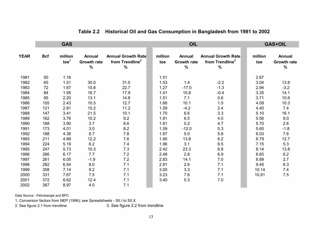
Table 2.2 Historical Oil and Gas Consumption in Bangladesh from 1981 to 2002

GAS OIL GAS+OIL

YEAR Bcf million Annual Annual Growth Rate million Annual Annual Growth Rate million Annual toe1 Growth rate from Trendline2 toe Growth rate from Trendline3 toe Growth rate

% % % % %

1981 50 1.16 1.51 2.671982 65 1.51 30.0 31.0 1.53 1.4 -2.2 3.04 13.81983 72 1.67 10.8 22.7 1.27 -17.0 -1.3 2.94 -3.21984 84 1.95 16.7 17.9 1.41 10.8 -0.4 3.35 14.11985 95 2.20 13.1 14.8 1.51 7.1 0.6 3.71 10.61986 105 2.43 10.5 12.7 1.66 10.1 1.5 4.09 10.31987 121 2.81 15.2 11.2 1.59 -4.2 2.4 4.40 7.41988 147 3.41 21.5 10.1 1.70 6.6 3.3 5.10 16.11989 162 3.76 10.2 9.2 1.81 6.5 4.0 5.56 9.01990 168 3.90 3.7 8.6 1.81 0.2 4.7 5.70 2.61991 173 4.01 3.0 8.2 1.59 -12.0 5.3 5.60 -1.81992 188 4.36 8.7 7.8 1.67 5.0 5.8 6.03 7.61993 211 4.89 12.2 7.6 1.90 13.8 6.2 6.79 12.71994 224 5.19 6.2 7.4 1.96 3.1 6.5 7.15 5.31995 247 5.73 10.3 7.3 2.42 23.3 6.8 8.14 13.81996 266 6.17 7.7 7.2 2.48 2.8 6.9 8.65 6.21997 261 6.05 -1.9 7.2 2.83 14.1 7.0 8.89 2.71998 282 6.54 8.0 7.1 2.91 2.6 7.1 9.45 6.31999 308 7.14 9.2 7.1 3.00 3.3 7.1 10.14 7.42000 331 7.67 7.5 7.1 3.23 7.6 7.1 10.91 7.52001 372 8.62 12.4 7.1 3.40 5.3 7.02002 387 8.97 4.0 7.1

Data Source - Petrobangla and BPC 1. Conversion factors from NEP (1996); see Spreadsheets - SII.I to SII.X2. See figure 2.1 from trendline 3. See figure 2.2 from trendline

13

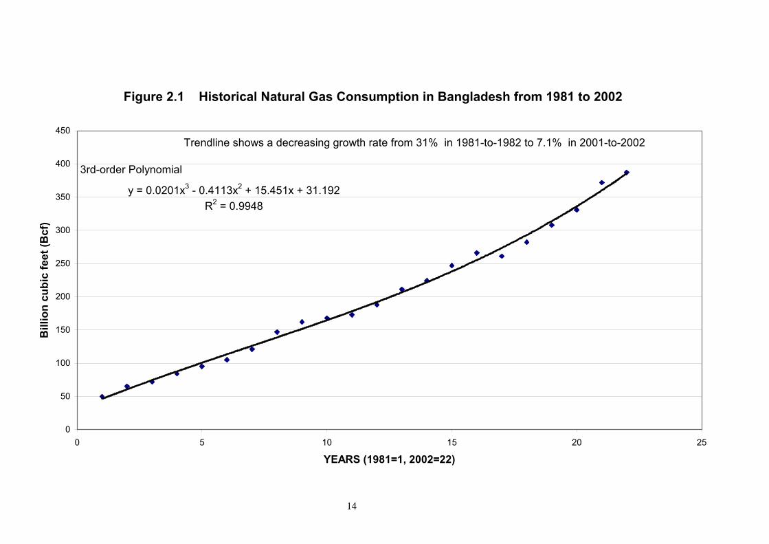
Figure 2.1 Historical Natural Gas Consumption in Bangladesh from 1981 to 2002

y = 0.0201x3 - 0.4113x2 + 15.451x + 31.192R2 = 0.9948

0

50

100

150

200

250

300

350

400

450

0 5 10 15 20 25

YEARS (1981=1, 2002=22)

Bill

ion

cubi

c fe

et (B

cf)

3rd-order Polynomial

Trendline shows a decreasing growth rate from 31% in 1981-to-1982 to 7.1% in 2001-to-2002

14

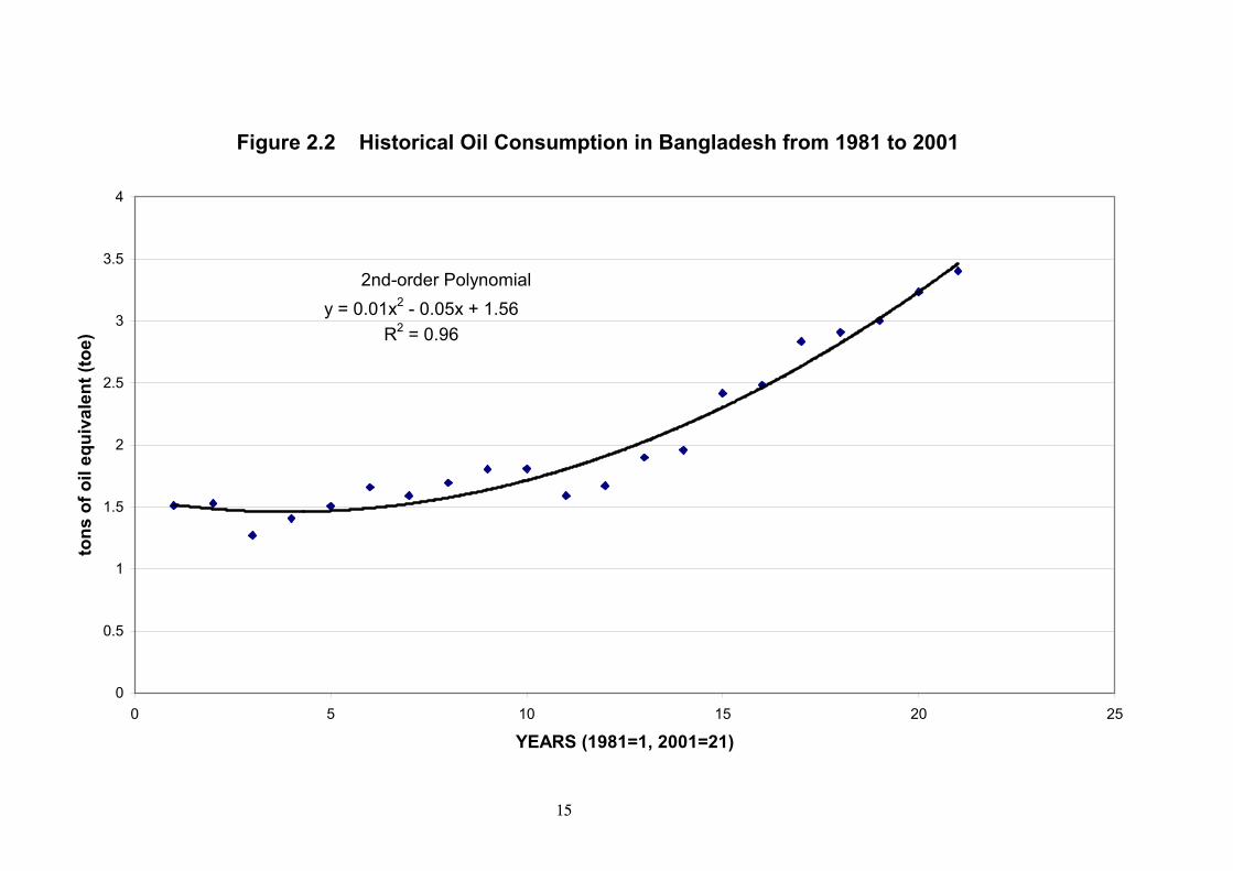
Figure 2.2 Historical Oil Consumption in Bangladesh from 1981 to 2001

y = 0.01x2 - 0.05x + 1.56R2 = 0.96

0

0.5

1

1.5

2

2.5

3

3.5

4

0 5 10 15 20 25

YEARS (1981=1, 2001=21)

tons

of o

il eq

uiva

lent

(toe

)

2nd-order Polynomial

15

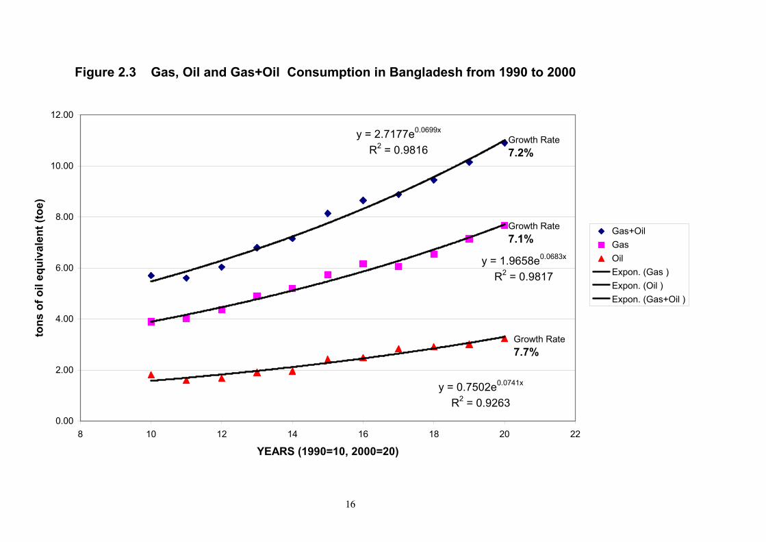
Figure 2.3 Gas, Oil and Gas+Oil Consumption in Bangladesh from 1990 to 2000

y = 1.9658e0.0683x

R2 = 0.9817

y = 0.7502e0.0741x

R2 = 0.9263

y = 2.7177e0.0699x

R2 = 0.9816

0.00

2.00

4.00

6.00

8.00

10.00

12.00

8 10 12 14 16 18 20 22

YEARS (1990=10, 2000=20)

tons

of o

il eq

uiva

lent

(toe

)

Gas+Oil Gas Oil Expon. (Gas )Expon. (Oil )Expon. (Gas+Oil )

Growth Rate 7.2%

Growth Rate 7.1%

Growth Rate 7.7%

16

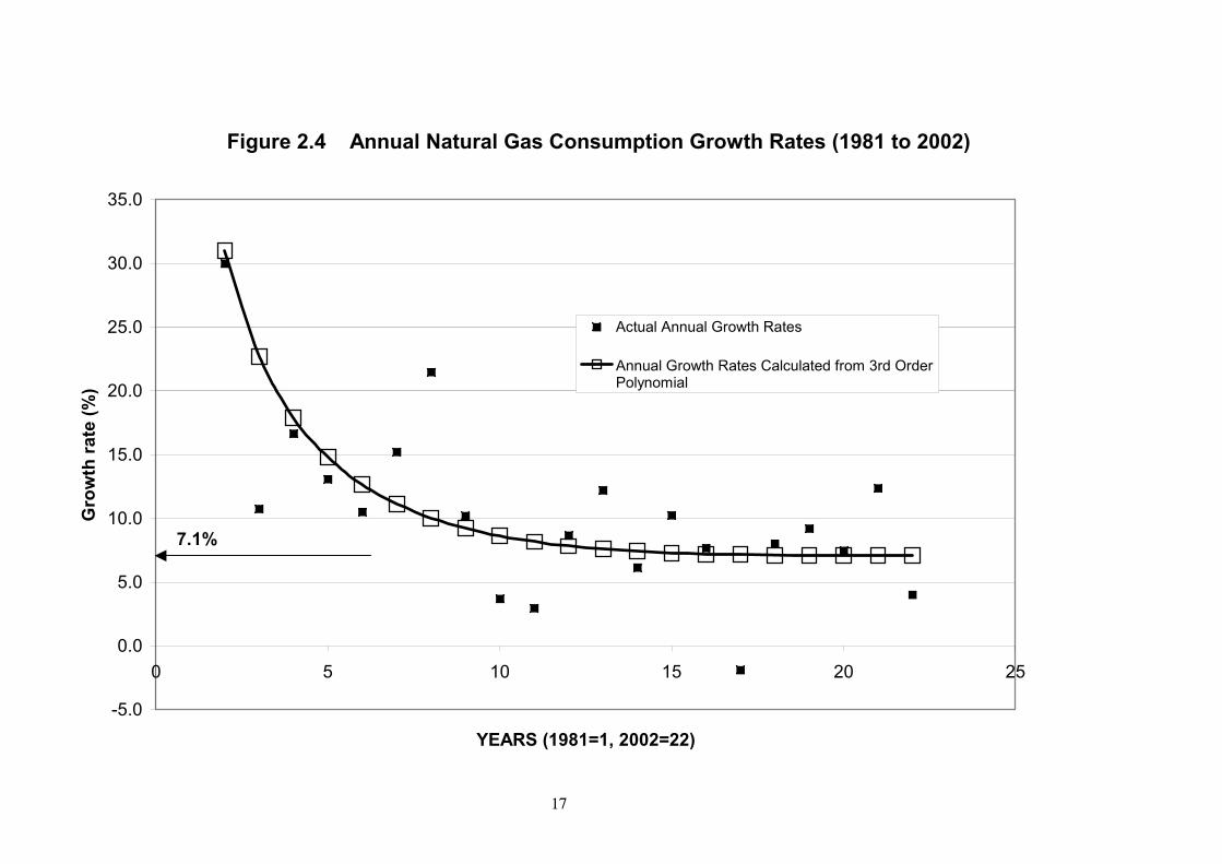
Figure 2.4 Annual Natural Gas Consumption Growth Rates (1981 to 2002)

-5.0

0.0

5.0

10.0

15.0

20.0

25.0

30.0

35.0

0 5 10 15 20 25

YEARS (1981=1, 2002=22)

Gro

wth

rate

(%)

Actual Annual Growth Rates

Annual Growth Rates Calculated from 3rd OrderPolynomial

7.1%

17

2000. However the plot of data from 1990 onwards shows that the growth

rate according to the exponential trendline has been steady at 7.1%

(ii) In the eighties annual oil consumption was constant. The growth rate in the

nineties according to the exponential trendline is 7.7%. However, the 7.7%

growth rate of oil is not the true historical growth rate because as is clearly

evident from Table 2.2 and Figure 2.2, there are some negative growth rates

in the eighties

(iii) The gas+oil, which constitute nearly 90% of commercial energy, growth rate

in the nineties has been a steady 7.2% according to the exponential trendline

of Figure 2.3. It is important to realize that this growth rate is from 1990 to

2000 and not the true historical growth rate.

2.4 Commercial Energy Demand Projection

2.4.1 General

The energy demand projection has been performed for 50 years on a total energy

requirement basis. No attempt has been made to disaggregate the total energy into sectoral

demand. To perform an energy demand projection using the GDP-Energy Intensity

methodology, the following two things are required during the planning period.

1. A model of EI

2. A prediction of GDP

It is obvious that the starting point for these should be historical data on energy and

GDP. Considering time and other limitations, the Committee found that it would be

most appropriate to work with the World Bank database as available in annually

published books known as the World Development Report (WDR) for the

commercial energy and the BBS for the GDP data in Taka. Thus data on population

and per capita commercial energy for the years between 1981 and 2000 were

collected from as many WDRs as the Committee could procure. The data collected

from the WDRs are shown in columns 2 and 3 of Table 2.3.

18

The WDR data have been used to calculate the commercial energy consumption as

shown in column 5 of Table 2.3. A plot of these data is given in Figure 2.5, which

shows that the total commercial energy in Bangladesh has been increasing at a

steady rate of 6.67% during the last two decades. It is instructive to compare

Figures 2.3 and 2.5. The slight lowering of growth rate is due to the fact that Figure

2.5 uses data for all commercial energy (including hydro and coal) from 1981. The

procedure followed to derive the GDP time series is explained in the following

section. The GDP and Total Energy values have been used to derive the Energy

Intensity (EI) values as shown in column 7 of Table 2.3. The full details of the

calculations performed in Table 2.3 can be found in BOX 1 termed – “Explanatory

Notes on Table 2.3”.

2.4.2 GDP Growth Rates

To use the energy intensity (EI) methodology for energy projection one must work with

constant GDP values. The Committee felt that it is most appropriate to work with as recent

data as possible, and therefore, chose 2000 as the base year. Since constant GDP values are

available in the BBS only for two base years, namely, 1984-85 and 1995-96, the Committee

had to find a way to generate the historical GDP values on a constant 2000 Taka basis. To

avoid laborious procedures of finding a deflator series for constant price GDP values for

2000, the Committee opted for the following simple procedure for generating past GDP

values.

The Committee decided to generate past GDP values using the following real GDP growth

rates as available in the latest World Bank publications (World Bank Website).

1980 to 1990 4.3%

1990 to 2000 4.8%

It is important to appreciate that these growth rates are constant Taka growth rates. The

World Bank merely reports the Bangladesh Bureau of Statistics data. The correctness of the

growth rates shown above has been confirmed from BBS publications (BBS, 1993 and BBS,

2002). Using these growth rates and the actual 2000 GDP (2371 billion Taka- BBS, 2002),

the GDP values for the years between 1981 and 1999 on a constant 2000 Taka have been

calculated as shown in Table 2.3 and Figure 2.6.

19

Figure 2.5 Historical Total Commercial Energy Consumption (1981 to 2000)

y = 3.0595e0.0646x

R2 = 0.9891

0.0

2.0

4.0

6.0

8.0

10.0

12.0

0 5 10 15 20 25

YEARS (1981=1, 2000=20)

Tota

l Com

mer

cial

Ene

rgy

(in to

e)

GROWTH RATE = 6.67 %

3.26

11.14

20

Table 2.3 Energy Database for Demand Projection

[1] [2] [3] [4] [5] [6] [7] Year Population Energy2 GDP1 Commercial YEAR Energy

per capita billion 2000 Taka Energy 1981=1 Intensity million kgoe (1981 to 1999 GDP values have million toe kgoe/Taka

(World Development Report Data) been generated from the actual 2000 values using GDP growth

rates shown below)

1981 90.7 34 1018 3.1 1 0.003031983 95.5 36 1108 3.4 3 0.003101985 100.6 43 1205 4.3 5 0.003591986 103.2 46 1257 4.7 6 0.003781987 106.1 47 1311 5.0 7 0.003801988 108.9 50 1367 5.4 8 0.003981990 106.7 57 1487 6.1 10 0.004091991 110.6 57 1555 6.3 11 0.004051992 114.4 59 1629 6.7 12 0.004141993 115.2 59 1708 6.8 13 0.003981994 117.9 64 1790 7.5 14 0.004221995 119.8 67 1876 8.0 15 0.004281997 124 71 2060 8.8 17 0.004271998 126 76 2159 9.6 18 0.004441999 128 81 2262 10.4 19 0.004582000 130 87 2371 11.3 20 0.00477

1. Year 2000 GDP is 2371 billion Taka. GDP growth rates: 4.3% - up to 1989, 4.55% - 1990, 4.8% - 1991 to 1999.

2. The per capita energy for the years 1997 to 2000 are Committee estimates from Bangladesh sources (see Table 2.2)

21

To join the two series 1980 to 1990 and 1990 to 2000, the annual growth rate between

1988-89 and 1989-90 was taken as the average of the two growth rates shown above, i.e.,

4.55%.

An exponential trendline was used for the generated GDP data shown in Figure 2.6, and as

may be expected the average annual growth rate was found to be 4.55%. Thus 4.55% has

been taken as the historical (20 years, 1980 to 2000) GDP growth rate trend, also called the

business-as-usual (BAU) trend. The BAU scenario, which says that the future is a reflection

of the past, is therefore 4.55% GDP growth in constant prices. At this point it is worth

clarifying two things. First, real growth rates can be used to generate constant Taka time

series for any base year because by definition real growth rate is independent of the base

year. The deflator series will of course be different for different base year, but real growth

rates calculated with any constant Taka time series would be the same. The second point

relates to the use of simulated as opposed to actual constant GDP values. As explained

earlier to generate actual 2000 time series data is simply not worth the effort because these

data are used only to calculate a suitable energy intensity model which can be projected into

the future. Moreover, the two EI models used in this work employs adjusted rather than

actual trend EI values. The Committee would like to emphasize that the purpose of this

entire exercise is an energy demand projection and NOT a GDP projection. The Committee

is making no comments on either past, present or future GDP growths, and is merely using

GDP as a parameter in the projections. It handles the delicate matter of future GDP

projections in the form of a sensitivity analysis.

The energy demand projection has been performed for GDP growth rates of 3.0, 4.55, 6.0

and 7.0%. All calculations have been performed using the constant 2000 Taka. Table 2.4

summarizes the GDP values for different growth rates for the years 2010, 2020, 2030, 2040

and 2050. Table 2.4 also gives the per capita GDP in constant 2000 Taka.

The Committee through a letter to the Secretary, Planning Commission requested for a

projection of GDP growth rates for Bangladesh in the next 50 years. Since no reply was

received to that request, the Committee opted for a large range of GDP values

22

Table 2.4 Projected GDP and Per Capita GDP at Different Growth Rates

2010 2020 2030 2040 2050 GDP, trillion 2000 Taka 3.19 4.28 5.76 7.73 10.39 3.0% Per capita GDP, 2000 T k

21435 25694 31416 39180 49845 GDP, trillion 2000 Taka 3.70 5.77 9.00 14.06 21.94 4.55% Per capita GDP, 2000 24888 34640 49176 71210 105187 GDP, trillion 2000 Taka 4.25 7.60 13.62 24.39 43.67 6.0% Per capita GDP, 2000 28563 45626 74337 123542 209437 GDP, trillion 2000 Taka 4.66 9.18 18.05 35.50 69.84 7.0% Per capita GDP, 2000 T k

31375 55051 98524 179859 334926

because members expressed the opinion that it is not possible to predict the growth rate of

Bangladesh economy in the next 48 years. The most likely scenario for any economy is

moderate growth interspersed by economic stagnation. However, the prospect of moderate to

high growth cannot be ruled out. It is outside the scope of the Committee’s work to comment

on what sort of economic growth Bangladesh will achieve. It is instructive to look at the GDP

values that have resulted from using the different GDP growth rates and draw conclusions

from those as to what Bangladesh is likely to achieve.

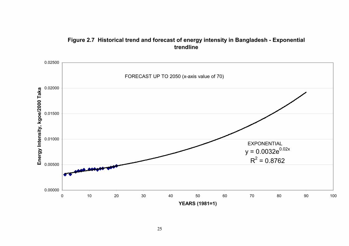
2.4.3 Energy Intensity Models

Plots of Energy intensity over time are shown in Figures 2.7 and 2.8. It is clear that the

energy intensity, which is calculated using real 2000 Taka, shows a clear increasing trend.

Figures 2.7 and 2.8 show linear and exponential trendlines for the data points. From a

visual observation it appears both linear and exponential trendlines are able to fit the data

points, with the exponential line fitting the recent points better. Figures 2.7 and 2.8 also

show how the trendlines would look if these were projected into the future (50 years is x-

axis value of 70). If the energy demand projection is done using the projected EI values as

shown in Figures 2.7 and 2.8 what one finds is that the exponential trendline predicts the

demand in the near term (say up to 2005) very well but gives a very large cumulative gas

requirement even for very low GDP growths: the linear trend on the other hand fails to

predict correctly the near term demand, but gives a reasonable future demand. These and

other considerations led the Committee to construct some realistic models for future energy

intensities.

23

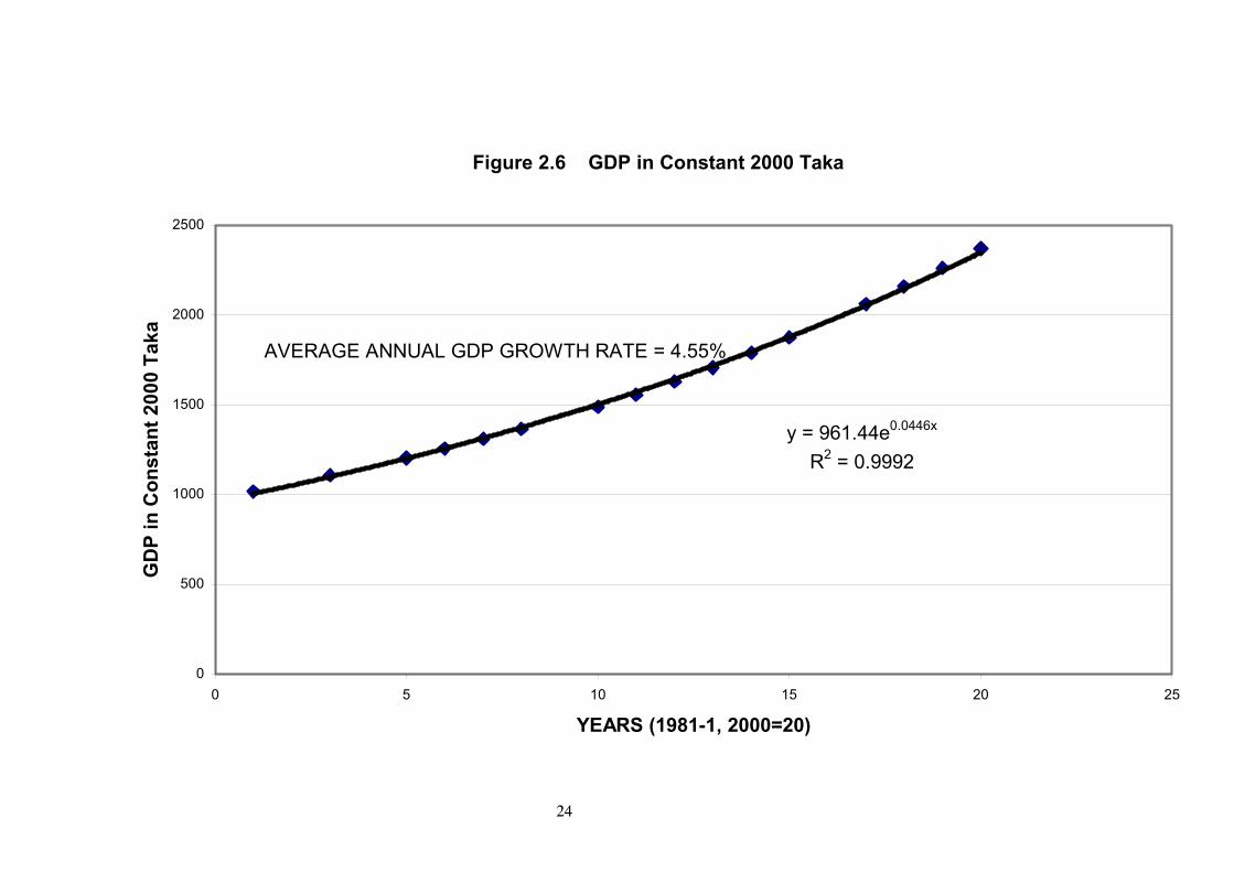
Figure 2.6 GDP in Constant 2000 Taka

y = 961.44e0.0446x

R2 = 0.9992

0

500

1000

1500

2000

2500

0 5 10 15 20 25

YEARS (1981-1, 2000=20)

GD

P in

Con

stan

t 200

0 Ta

ka

AVERAGE ANNUAL GDP GROWTH RATE = 4.55%

24

25

Figure 2.7 Historical trend and forecast of energy intensity in Bangladesh - Exponential trendline

y = 0.0032e0.02x

R2 = 0.8762

0.00000

0.00500

0.01000

0.01500

0.02000

0.02500

0 10 20 30 40 50 60 70 80 90 100

YEARS (1981=1)

Ener

gy In

tens

ity, k

goe/

2000

Tak

a

FORECAST UP TO 2050 (x-axis value of 70)

EXPONENTIAL

Figure 2.8 Historical trend and forecast of energy intensity in Bangladesh - Linear trendline

y = 8E-05x + 0.0031R2 = 0.9032

0.00000

0.00200

0.00400

0.00600

0.00800

0.01000

0.01200

0 10 20 30 40 50 60 70 80 90 100

YEARS (1981=1)

Ener

gy In

tens

ity, k

goe/

2000

Tak

a

FORECAST UP TO 2050 (x-axis value of 70)

LINEAR

26

Two models of energy intensity along with the exponential and linear trendlines

(labeled Model I and Model II) are shown in Figure 2.9, and the essential features

of those are summarized in Table 2.5. Models III and IV have been constructed in

such a way that the projected energy demands using these EI models yield realistic

values of cumulative gas requirement. These models in the first phase (15 years for

Model III and 5 years for Model IV) retain the exponential trend, after which the

shapes of these curves have been adjusted as shown in Figure 2.9 using expert

judgement. Model III reaches a maximum value at 2020, while Model IV reaches its

maximum value at 2015. The peak value of Model III is approximately 16% higher

than that of Model IV. The energy intensity in both these remain at the peak value

for about 5 years before descending to a common 2050 value. The rationale behind

these models is that as the economy matures, energy growth rate decreases. These

parabolic shaped curves are well known to energy analysts.

Table 2.5 Summary of the Energy Intensity1 Models used for the Projections

Energy Intensity Models

Exponential

up to YEAR

Peak value

of EI

2050 value

of EI

MODEL I EXPONENTIAL 2050 .01298 .01298

MODEL II LINEAR NA .0087 .0087

MODEL III ADJUSTED – HIGH 2015 .00677 .00383

MODEL IV ADJUSTED – LOW 2005 .00583 .00383 1 Energy intensity unit is kgoe/ 2000 Taka, see Figure 2.9

2.4.4 Energy Demand Projection

Using the Energy Intensity Models I to IV, energy demand projections up to the

year 2050 have been performed using Excel spreadsheets. The details of the

calculation methodology and the assumptions used for the demand projections are

presented in Box 2 titled “Calculation Methodology for the Energy Projection

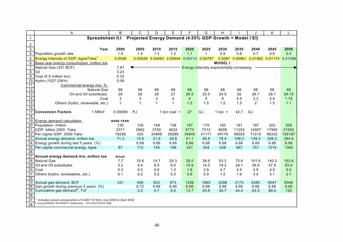
Spreadsheets”. Spreadsheet II.I presents the calculation using Model I EI for the

business-as-usual 4.55% GDP growth in real or constant 2000 Taka.

27

Figure 2.9 Energy Intensity Models

0

0.002

0.004

0.006

0.008

0.01

0.012

0.014

2000 2010 2020 2030 2040 2050 2060

YEARS

Ener

gy In

tens

ity, k

goe/

2000

Tak

a

MODEL IExponential

MODEL II Linear

MODEL III Adjusted - High

MODEL IV Adjusted - Low

28

2050 even for the 4.55% GDP growth is 125 Tcf as can be seen from Figure 2.10.

As remarked earlier, the Committee felt that the EI value of 0.01298 kgoe/2000

Taka in 2050 (see Model I in Figure 2.9) is too high. Therefore, no other GDP

scenarios were constructed with the exponential EI model.

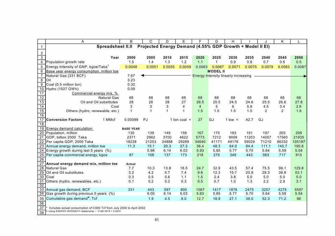
The spreadsheet for the linear model using the 4.55% GDP growth is presented in

Spreadsheet II.II. The gas requirement in 2050 is predicted to be 96 Tcf as can be

seen from Figure 2.11. This model has two deficiencies. First, it gives a high 50-

year gas requirement, and second, compared to the prevailing actual gas growth

rates (2001 and 2002), it under-predicts the gas requirement in the first few years of

the prediction. Both the exponential and linear EI model scenarios give high growth

rates of gas throughout the planning period. The Committee was of the opinion that

a high growth rate (between 6 and 7%) in the early years and a low growth rate

(between 1 and 2%) in the later years is more representative of the Bangladesh

reality. Thus, it was felt that it is not worth constructing other scenarios with the

linear model of EI.

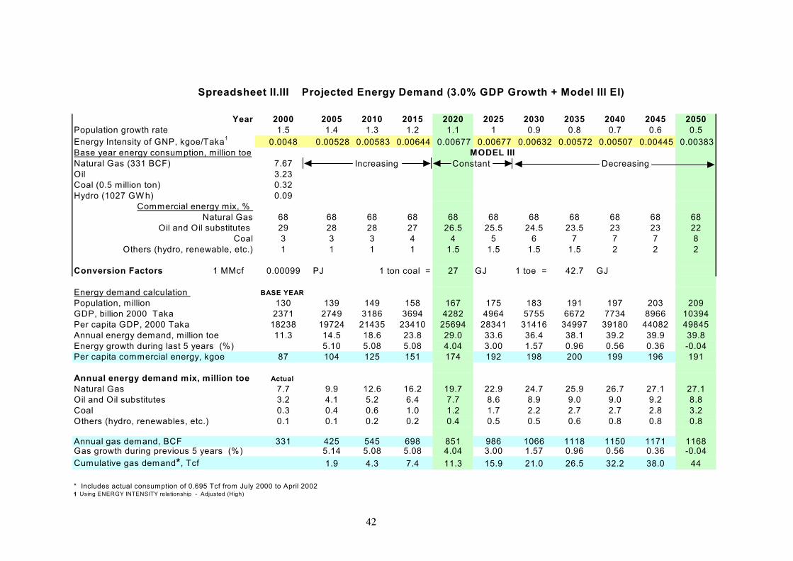
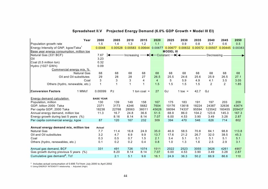
The energy demand prediction using Models III and IV are presented in eight

spreadsheets and two graphs (Figures 2.12 and 2.13). The 6 and 7% GDP growth

rates allow for the possibility of Bangladesh economy doing better than the business-

as-usual case of 4.55%. This is desirable but will certainly not be easily achievable

because with every passing year the size of the economy is growing. To achieve a

7% growth in 2040 when the economy size is 36 trillion in 2000 Taka (year 2000

economy size is 2.4 trillion Taka) will certainly not be easy because Bangladesh is

failing to achieve that kind of growth even when the economy size is small.

The 3.0% growth scenario is included to reflect the possibility of low growth and or

stagnation and recession during the 50-year period. It must be remembered that

probably no country in the world has achieved continuous economic growth for 80

years as predicated by the models. The 80 years comes about from the fact that

Bangladesh has already achieved 30 years of growth with no stagnation or recession

since its independence. Moreover, if one looks at the constant per capita GDP

values at 2050, it should become obvious that even continuous 3% growth for 50

years will deliver a considerable amount of prosperity to the nation. 29

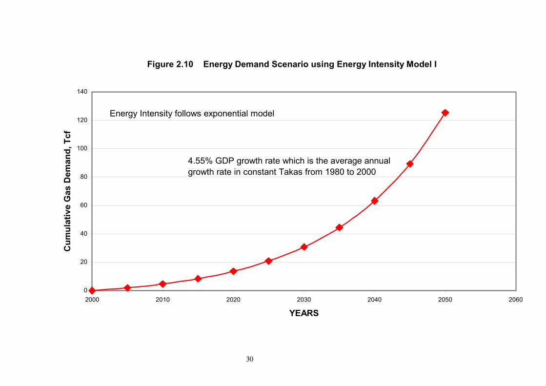
Figure 2.10 Energy Demand Scenario using Energy Intensity Model I

0

20

40

60

80

100

120

140

2000 2010 2020 2030 2040 2050 2060

YEARS

Cum

ulat

ive

Gas

Dem

and,

Tcf

4.55% GDP growth rate which is the average annual growth rate in constant Takas from 1980 to 2000

Energy Intensity follows exponential model

30

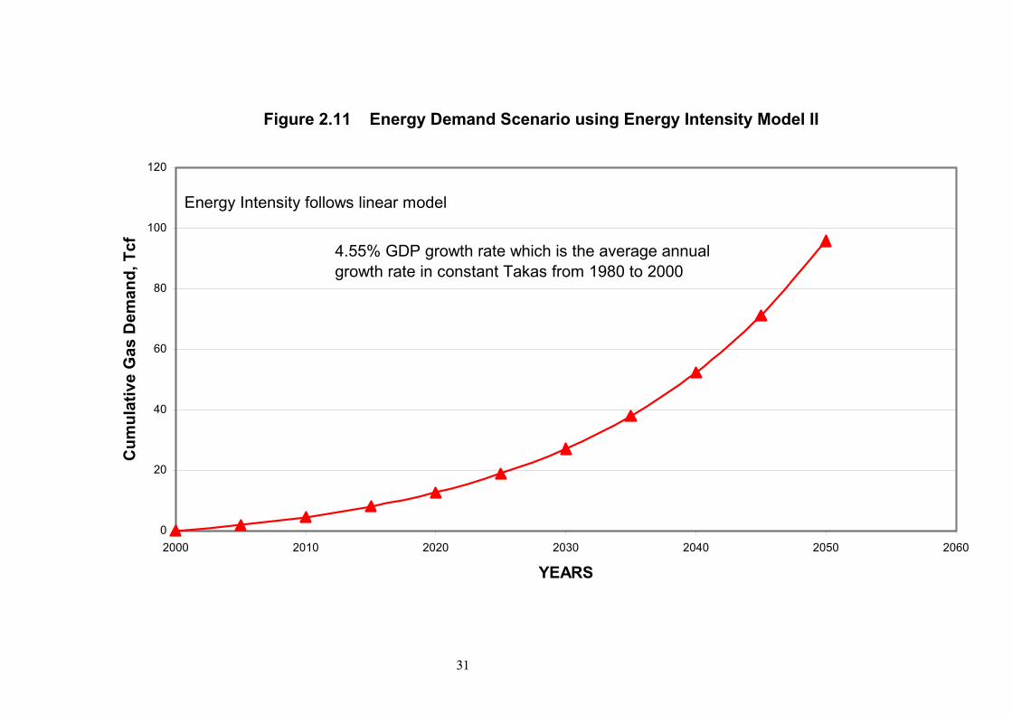
Figure 2.11 Energy Demand Scenario using Energy Intensity Model II

0

20

40

60

80

100

120

2000 2010 2020 2030 2040 2050 2060

YEARS

Cum

ulat

ive

Gas

Dem

and,

Tcf

Energy Intensity follows linear model

4.55% GDP growth rate which is the average annual growth rate in constant Takas from 1980 to 2000

31

Figure 2.12 Energy Demand Scenarios using Energy Intensity Model III

0

20

40

60

80

100

120

140

160

2000 2010 2020 2030 2040 2050 2060

YEARS

Cum

ulat

ive

Gas

Dem

and,

Tcf

4.55%

7.0%

3.0%

4.55% is 1980-2000 Average Annual GDP Growth Rate in Constant Taka

6.0%

32

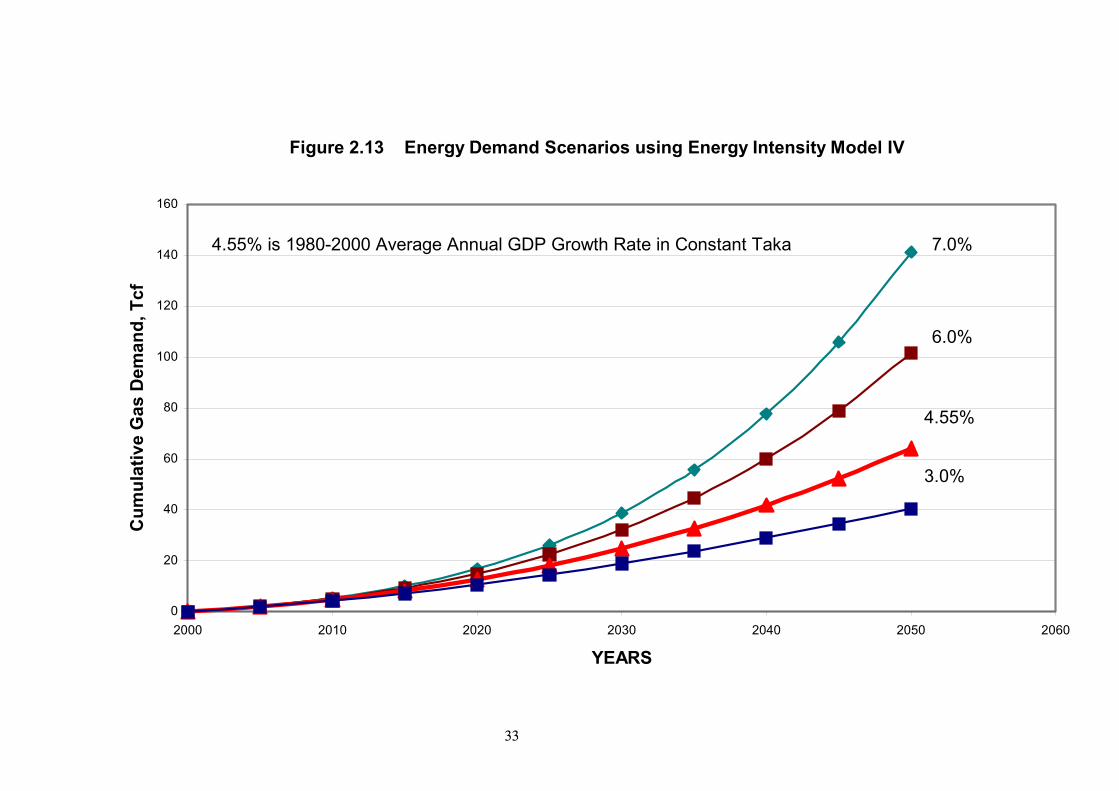
Figure 2.13 Energy Demand Scenarios using Energy Intensity Model IV

0

20

40

60

80

100

120

140

160

2000 2010 2020 2030 2040 2050 2060

YEARS

Cum

ulat

ive

Gas

Dem

and,

Tcf

4.55%

6.0%

7.0%

3.0%

4.55% is 1980-2000 Average Annual GDP Growth Rate in Constant Taka

33

Table 2.6 presents a summarized version of the results given in the 10 spreadsheets.

These results should be treated as a sensitivity analysis of the GDP. Using these

values of the matrix one can construct probable scenarios for the future for possible

growth rates between 3 and 7%. It is worth pointing out that because the modelling

starts at the year 2000 the results of the 3% and 7% scenarios will not totally reflect

reality because these do not match the actual growth rates of the last two years. In

fact one can expect that at least up to 2010 these will not match reality. The

projected 2050 energy demands for fixed GDP growth rates will therefore be under

prediction for the 3% scenario and over prediction for the 7% scenario. However,

as pointed out earlier these are sensitivity analysis values and should be interpreted

thus.

From Table 2.6 it can be seen that the gas requirement varies between 64 and 69 Tcf in the

business-as-usual (BAU) scenario when realistic models of energy intensities are used. In the

scenario where the energy intensity keeps on increasing exponentially, the requirement is 125

Tcf even in the BAU GDP growth case. It is instructive to compare these values with the

Petrobangla’s natural gas projection for 50 years. By consulting Table 2.6 one can conclude

that the projection more or less matches the BAU growth scenarios with realistic EI models.

The BAU scenarios’ gas growth rates along with those of the Petrobangla’s Projection are

presented in Table 2.7. The most noteworthy feature, which allows the logic for rejecting

Model I to be clearly appreciated, is that the exponential model predicts a constant 6.7%

annual gas demand growth rate up to 2050. The linear model also predicts high gas demand

growth rates all through the 50 years planning period. Considering the fact that during the last

two decades Bangladesh has already experienced very high gas growth rates, it is highly

unlikely that gas demand growth rates of 5.6 to 6.7% will be sustained for the next 50 years.

Model III and Model IV predict declining gas demand growth rates. Petrobangla’s 50-year

projection predicts high growth rates in the first two decades and very low growth rates in the

last two decades. From the analysis performed here, such a scenario cannot be constructed

unless in the last two decades the models use very low GDP growth rates or energy intensity

values.

34

Table 2.6 Summary of the Projected Natural Gas Demand Cumulative Gas Demand in Tcf GDP Growth

Rate 2010 2020 2030 2040 2050

Model I (Exponential) 4.55% 4.7 13.7 30.7 63.3 125

Model II (Linear) 4.55% 4.5 12.7 27.1 52.3 96

3.0% 4.3 11.3 21.0 32.2 44

4.55% 4.7 13.5 27.7 46.6 69

6.0% 5.1 16.1 36.3 66.9 110

Model III (Adjusted – High) (Exponential up to 2015, increase up to 2020, constant up to 2025, steady decrease up to EI value of 0.00383 kgoe/2000 Taka)

7.0% 5.4 18.1 43.8 86.6 152

3.0% 4.3 10.6 18.9 29.0 40

4.55% 4.7 12.6 24.7 41.8 64

6.0% 5.0 14.9 32.2 60.0 101

Model IV (Adjusted – Low) (Exponential up to 2005, slow increase up to 2015, constant up to 2020, steady decrease up to EI value of 0.00383 kgoe/2000 Taka)

7.0% 5.3 16.8 38.8 77.7 141

Petrobangla’s Projection 4.8 13.7 26.8 43.7 63

Table 2.7 Annual Natural Gas Demand Growth Rates Every Ten Years for the 4.55% GDP Growth Rate Under Different Energy Intensity Scenarios

Annual Gas Demand Growth Rate (%)

SCENARIOS 2000-10 2010-20 2020-30 2030-40 2040-50

Model I (Exponential) 6.7 6.7 6.7 6.7 6.7

Model II (Linear) 6.1 6.0 5.8 5.7 5.6

Model III (Adjusted – High) 6.7 6.1 3.8 2.3 1.7

Model IV (Adjusted – Low)

6.4 4.9 3.9 3.1 2.3

Petrobangla’s Projection 5.9 5.3 3.4 1.6 0.9

2.5 Conclusions

1. The usefulness of several scenarios is that one can readily get a picture of the energy

requirement given a level of economic performance. The natural gas requirement in the next

50 years starting from the year 2000 may be summarized as follows:

• If the economic performance is on the low side (3% GDP growth rate), the total

gas requirement will be between 40 and 44 Tcf.

35

•

•

•

If economic performance continues according to the historical trend (Business-

as-usual; 4.55% GDP growth rate), gas requirement will be between 64 and 69

Tcf.

If performance is on the moderately high side (6% GDP growth rate), gas


If performance is on the high side (7% GDP growth rate), gas requirement will

be between 141 and 152 Tcf.

2. It must be emphasized that these scenarios imply a sustained level of performance over the

entire 50 years. Whereas it may be quite possible for Bangladesh to achieve a 7% real Taka

GDP growth when the economy size is small, but achieving the same when the size of the

economy is large, say 8 to 10 times the present size of about 2.4 trillion Taka will certainly

not be easy. However, a large economy achieving a 7% or more growth is not an unheard

off thing. It is worth noting that even for the 4.55% GDP growth rate, the real per capita

income becomes Taka 105187. This is no mean performance, because it implies that if the

present day population were 209 million (the assumed 2050 population), every citizen would

have a per capita income of 105187 in 2000 constant Taka (nearly six times the 2000 per

capita income of Taka 18238).

3. It has been stated earlier that the energy requirement of the future will be crucially

dependent on what economic growth Bangladesh manages to achieve. Since the Committee

cannot predict the future economic performance of Bangladesh, it is constrained to present

the Demand Projections in the form of different scenarios. The Committee would like to

point out that if economic growth is high, energy demand will be high, but if economic

growth is low, energy demand will be correspondingly low. The Committee is able to state

with a reasonable level of certainty that the energy requirements given in Table 2.6 for

different growth rates of GDP may be used for planning purposes. It is highly unlikely

given the large range of predictions that the actual demand in the country will go outside

this range unless unforeseen things dominate the global energy scenario.

36

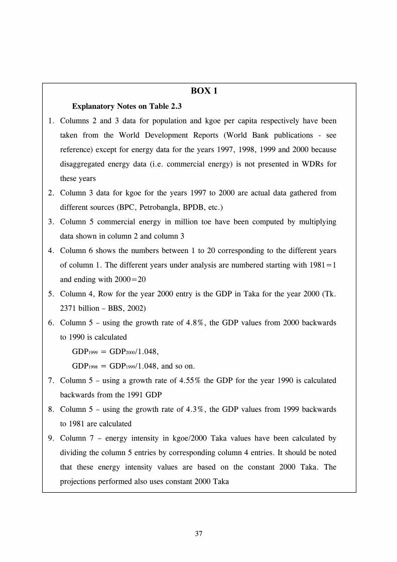
BOX 1 Explanatory Notes on Table 2.3

1. Columns 2 and 3 data for population and kgoe per capita respectively have been

taken from the World Development Reports (World Bank publications - see

reference) except for energy data for the years 1997, 1998, 1999 and 2000 because

disaggregated energy data (i.e. commercial energy) is not presented in WDRs for

these years

2. Column 3 data for kgoe for the years 1997 to 2000 are actual data gathered from

different sources (BPC, Petrobangla, BPDB, etc.)

3. Column 5 commercial energy in million toe have been computed by multiplying

data shown in column 2 and column 3

4. Column 6 shows the numbers between 1 to 20 corresponding to the different years

of column 1. The different years under analysis are numbered starting with 1981=1

and ending with 2000=20

5. Column 4, Row for the year 2000 entry is the GDP in Taka for the year 2000 (Tk.

2371 billion – BBS, 2002)

6. Column 5 – using the growth rate of 4.8%, the GDP values from 2000 backwards

to 1990 is calculated

GDP1999 = GDP2000/1.048,

GDP1998 = GDP1999/1.048, and so on.

7. Column 5 – using a growth rate of 4.55% the GDP for the year 1990 is calculated

backwards from the 1991 GDP

8. Column 5 – using the growth rate of 4.3%, the GDP values from 1999 backwards

to 1981 are calculated

9. Column 7 – energy intensity in kgoe/2000 Taka values have been calculated by

dividing the column 5 entries by corresponding column 4 entries. It should be noted

that these energy intensity values are based on the constant 2000 Taka. The

projections performed also uses constant 2000 Taka

37

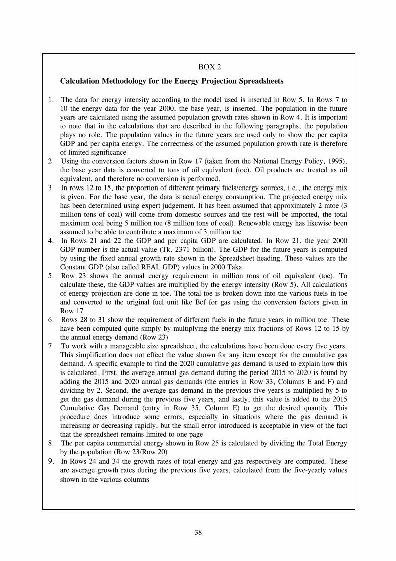
BOX 2

Calculation Methodology for the Energy Projection Spreadsheets

1. The data for energy intensity according to the model used is inserted in Row 5. In Rows 7 to 10 the energy data for the year 2000, the base year, is inserted. The population in the future years are calculated using the assumed population growth rates shown in Row 4. It is important to note that in the calculations that are described in the following paragraphs, the population plays no role. The population values in the future years are used only to show the per capita GDP and per capita energy. The correctness of the assumed population growth rate is therefore of limited significance

2. Using the conversion factors shown in Row 17 (taken from the National Energy Policy, 1995), the base year data is converted to tons of oil equivalent (toe). Oil products are treated as oil equivalent, and therefore no conversion is performed.

3. In rows 12 to 15, the proportion of different primary fuels/energy sources, i.e., the energy mix is given. For the base year, the data is actual energy consumption. The projected energy mix has been determined using expert judgement. It has been assumed that approximately 2 mtoe (3 million tons of coal) will come from domestic sources and the rest will be imported, the total maximum coal being 5 million toe (8 million tons of coal). Renewable energy has likewise been assumed to be able to contribute a maximum of 3 million toe

4. In Rows 21 and 22 the GDP and per capita GDP are calculated. In Row 21, the year 2000 GDP number is the actual value (Tk. 2371 billion). The GDP for the future years is computed by using the fixed annual growth rate shown in the Spreadsheet heading. These values are the Constant GDP (also called REAL GDP) values in 2000 Taka.

5. Row 23 shows the annual energy requirement in million tons of oil equivalent (toe). To calculate these, the GDP values are multiplied by the energy intensity (Row 5). All calculations of energy projection are done in toe. The total toe is broken down into the various fuels in toe and converted to the original fuel unit like Bcf for gas using the conversion factors given in Row 17

6. Rows 28 to 31 show the requirement of different fuels in the future years in million toe. These have been computed quite simply by multiplying the energy mix fractions of Rows 12 to 15 by the annual energy demand (Row 23)

7. To work with a manageable size spreadsheet, the calculations have been done every five years. This simplification does not effect the value shown for any item except for the cumulative gas demand. A specific example to find the 2020 cumulative gas demand is used to explain how this is calculated. First, the average annual gas demand during the period 2015 to 2020 is found by adding the 2015 and 2020 annual gas demands (the entries in Row 33, Columns E and F) and dividing by 2. Second, the average gas demand in the previous five years is multiplied by 5 to get the gas demand during the previous five years, and lastly, this value is added to the 2015 Cumulative Gas Demand (entry in Row 35, Column E) to get the desired quantity. This procedure does introduce some errors, especially in situations where the gas demand is increasing or decreasing rapidly, but the small error introduced is acceptable in view of the fact that the spreadsheet remains limited to one page

8. The per capita commercial energy shown in Row 25 is calculated by dividing the Total Energy by the population (Row 23/Row 20)

9. In Rows 24 and 34 the growth rates of total energy and gas respectively are computed. These are average growth rates during the previous five years, calculated from the five-yearly values shown in the various columns

38

2.6 References

1. BBS, 1993, “Twenty Years of National Accounting of Bangladesh

(1972-73 to 1991-92)”, Bangladesh Bureau of Statistics, Ministry of Planning, Government of People’s Republic of Bangladesh, Dhaka, Bangladesh, July 1993.

2. BBS, 2002, Statistical Pocketbook of Bangladesh 2000.

3. BPC, personal communication.

4. Khan, M.A. Aziz (2001), Natural Gas Demand and Supply Forecast: Bangladesh (FY 2001 to 2050), Bangladesh Oil, Gas and Mineral Corporation (Petrobangla), Petro Centre, 3 Karwan Bazar, Dhaka, 15 March 2001.

5. Petrobangla, personal communication.

6. National Energy Policy (NEP), GOB, (1996).

7. World Bank Website – www.worldbank.org.

8. World Development Report, 1983, World Bank.











19. World Development Report. 1997, World Bank.

20. World Development Report, 1989/99, World Bank.




39

http://www.worldbank.org/

1

23456789

1011121314151617181920212223242526272829303132333435363738

A B C D E F G H I J K LSpreadsheet II.I Projected Energy Demand (4.55% GDP Growth + Model I EI)

Year 2000 2005 2010 2015 2020 2025 2030 2035 2040 2045 2050Population growth rate 1.5 1.4 1.3 1.2 1.1 1 0.9 0.8 0.7 0.6 0.5Energy Intensity of GDP, kgoe/Taka1 0.0048 0.00528 0.00583 0.00644 0.00712 0.00787 0.0087 0.00961 0.01062 0.01174 0.01298Base year energy consumption, million toe MODEL I Natural Gas (331 BCF) 7.67 Energy Intensity exponentially increasing Oil 3.23Coal (0.5 million ton) 0.32Hydro (1027 GWh) 0.09

Commercial energy mix, % Natural Gas 68 68 68 68 68 68 68 68 68 68 68

Oil and Oil substitutes 29 28 28 27 26.5 25.5 24.5 26 26.7 28.1 29.15Coal 3 3 3 4 4 5 6 4.5 3.3 2.4 1.75

Others (hydro, renewable, etc.) 1 1 1 1 1.5 1.5 1.5 1.5 2 1.5 1.1

Conversion Factors 1 MMcf 0.00099 PJ 1 ton coal = 27 GJ 1 toe = 42.7 GJ

Energy demand calculation BASE YEAR Population, million 130 139 149 158 167 175 183 191 197 203 209GDP, billion 2000 Taka 2371 2962 3700 4622 5773 7212 9009 11253 14057 17560 21935Per capita GDP, 2000 Taka 18238 425 24888 29289 34640 41171 49176 59029 71210 86332 105187Annual energy demand, million toe 11.3 15.6 21.6 29.8 41.1 56.8 78.4 108.2 149.3 206.2 284.6Energy growth during last 5 years (%) 6.68 6.66 6.66 6.66 6.66 6.66 6.66 6.66 6.66 6.66Per capita commercial energy, kgoe 87 112 145 189 247 324 428 567 757 1014 1365

Annual energy demand mix, million toe Actual Natural Gas 7.7 10.6 14.7 20.3 28.0 38.6 53.3 73.6 101.6 140.2 193.6Oil and Oil substitutes 3.2 4.4 6.0 8.0 10.9 14.5 19.2 28.1 39.9 57.9 83.0Coal 0.3 0.5 0.6 1.2 1.6 2.8 4.7 4.9 4.9 4.9 5.0Others (hydro, renewables, etc.) 0.1 0.2 0.2 0.3 0.6 0.9 1.2 1.6 3.0 3.1 3.1

Annual gas demand, BCF 331 458 633 873 1206 1665 2298 3173 4380 6047 8348Gas growth during previous 5 years (%) 6.72 6.66 6.66 6.66 6.66 6.66 6.66 6.66 6.66 6.66Cumulative gas demand*, Tcf 2.0 4.7 8.5 13.7 20.8 30.7 44.4 63.3 89.4 125

* Includes actual consumption of 0.695 Tcf from July 2000 to April 2002 1 Using ENERGY INTENSITY relationship - Y=0.0032*EXP(0.02X)

40

1

23456789

1011121314151617181920212223242526272829303132333435363738

A B C D E F G H I J K LSpreadsheet II.II Projected Energy Demand (4.55% GDP Growth + Model II EI)

Year 2000 2005 2010 2015 2020 2025 2030 2035 2040 2045 2050Population growth rate 1.5 1.4 1.3 1.2 1.1 1 0.9 0.8 0.7 0.6 0.5Energy Intensity of GNP, kgoe/Taka1 0.0048 0.0051 0.0055 0.0059 0.0063 0.0067 0.0071 0.0075 0.0079 0.0083 0.0087Base year energy consumption, million toe MODEL II Natural Gas (331 BCF) 7.67 Energy Intensity linearly increasing Oil 3.23Coal (0.5 million ton) 0.32Hydro (1027 GWh) 0.09


Oil and Oil substitutes 29 28 28 27 26.5 25.5 24.5 24.6 25.5 26.6 27.8Coal 3 3 3 4 4 5 6 5.9 4.5 3.4 2.6

Others (hydro, renewable, etc.) 1 1 1 1 1.5 1.5 1.5 1.5 2 2 1.6





* Includes actual consumption of 0.695 Tcf from July 2000 to April 2002 1 Using ENERGY INTENSITY relationship - Y=8E-05*X + 0.0031

41

Spreadsheet II.III Projected Energy Demand (3.0% GDP Growth + Model III EI)

Year 2000 2005 2010 2015 2020 2025 2030 2035 2040 2045 2050Population growth rate 1.5 1.4 1.3 1.2 1.1 1 0.9 0.8 0.7 0.6 0.5Energy Intensity of GNP, kgoe/Taka1 0.0048 0.00528 0.00583 0.00644 0.00677 0.00677 0.00632 0.00572 0.00507 0.00445 0.00383Base year energy consumption, million toe MODEL III Natural Gas (331 BCF) 7.67Oil 3.23Coal (0.5 million ton) 0.32Hydro (1027 GW h) 0.09


Oil and Oil substitutes 29 28 28 27 26.5 25.5 24.5 23.5 23 23 22Coal 3 3 3 4 4 5 6 7 7 7 8

Others (hydro, renewable, etc.) 1 1 1 1 1.5 1.5 1.5 1.5 2 2 2


Energy demand calculation BASE YEAR Population, million 130 139 149 158 167 175 183 191 197 203 209GDP, billion 2000 Taka 2371 2749 3186 3694 4282 4964 5755 6672 7734 8966 10394Per capita GDP, 2000 Taka 18238 19724 21435 23410 25694 28341 31416 34997 39180 44082 49845Annual energy demand, million toe 11.3 14.5 18.6 23.8 29.0 33.6 36.4 38.1 39.2 39.9 39.8Energy growth during last 5 years (%) 5.10 5.08 5.08 4.04 3.00 1.57 0.96 0.56 0.36 -0.04Per capita commercial energy, kgoe 87 104 125 151 174 192 198 200 199 196 191


Annual gas demand, BCF 331 425 545 698 851 986 1066 1118 1150 1171 1168Gas growth during previous 5 years (%) 5.14 5.08 5.08 4.04 3.00 1.57 0.96 0.56 0.36 -0.04Cumulative gas demand*, Tcf 1.9 4.3 7.4 11.3 15.9 21.0 26.5 32.2 38.0 44

* Includes actual consumption of 0.695 Tcf from July 2000 to April 2002 1 Using ENERGY INTENSITY relationship - Adjusted (High)

Increasing Constant Decreasing

42

Spreadsheet II.IV Projected Energy Demand (4.55% GDP Growth + Model III EI)

Year 2000 2005 2010 2015 2020 2025 2030 2035 2040 2045 2050Population growth rate 1.5 1.4 1.3 1.2 1.1 1 0.9 0.8 0.7 0.6 0.5Energy Intensity of GNP, kgoe/Taka1 0.0048 0.00528 0.00583 0.00644 0.00677 0.00677 0.00632 0.00572 0.00507 0.00445 0.00383Base year energy consumption, million toe MODEL III Natural Gas (331 BCF) 7.67Oil 3.23Coal (0.5 million ton) 0.32Hydro (1027 GWh) 0.09


Oil and Oil substitutes 29 28 28 27 26.5 25.5 24.5 23.5 23 23.6 24Coal 3 3 3 4 4 5 6 7 7 6.4 6








43

Spreadsheet II.V Projected Energy Demand (6.0% GDP Growth + Model III EI)

Year 2000 2005 2010 2015 2020 2025 2030 2035 2040 2045 2050Population growth rate 1.5 1.4 1.3 1.2 1.1 1 0.9 0.8 0.7 0.6 0.5Energy Intensity of GNP, kgoe/Taka1 0.0048 0.00528 0.00583 0.00644 0.00677 0.00677 0.00632 0.00572 0.00507 0.00445 0.00383Base year energy consumption, million toe MODEL III Natural Gas (331 BCF) 7.67Oil 3.23Coal (0.5 million ton) 0.32Hydro (1027 GW h) 0.09


Oil and Oil substitutes 29 28 28 27 26.5 25.5 24.6 25.6 25.9 26.5 27.1Coal 3 3 3 4 4 5 5.9 4.9 4.1 3.5 3.05








44

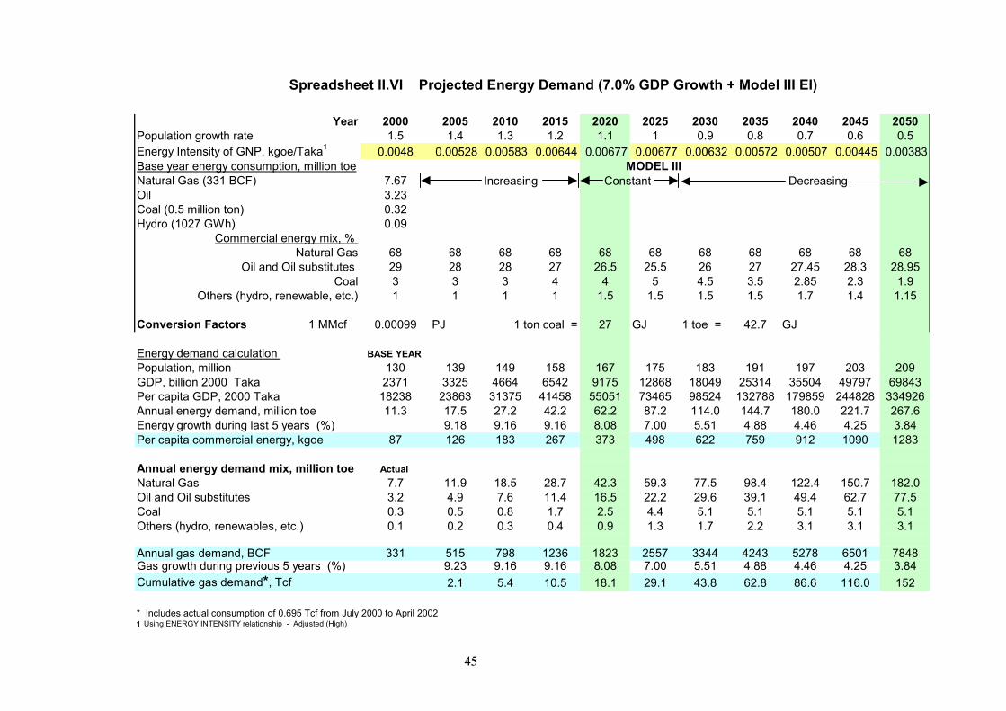
Spreadsheet II.VI Projected Energy Demand (7.0% GDP Growth + Model III EI)

Year 2000 2005 2010 2015 2020 2025 2030 2035 2040 2045 2050Population growth rate 1.5 1.4 1.3 1.2 1.1 1 0.9 0.8 0.7 0.6 0.5Energy Intensity of GNP, kgoe/Taka1 0.0048 0.00528 0.00583 0.00644 0.00677 0.00677 0.00632 0.00572 0.00507 0.00445 0.00383Base year energy consumption, million toe MODEL III Natural Gas (331 BCF) 7.67Oil 3.23Coal (0.5 million ton) 0.32Hydro (1027 GWh) 0.09


Oil and Oil substitutes 29 28 28 27 26.5 25.5 26 27 27.45 28.3 28.95Coal 3 3 3 4 4 5 4.5 3.5 2.85 2.3 1.9

Others (hydro, renewable, etc.) 1 1 1 1 1.5 1.5 1.5 1.5 1.7 1.4 1.15







45

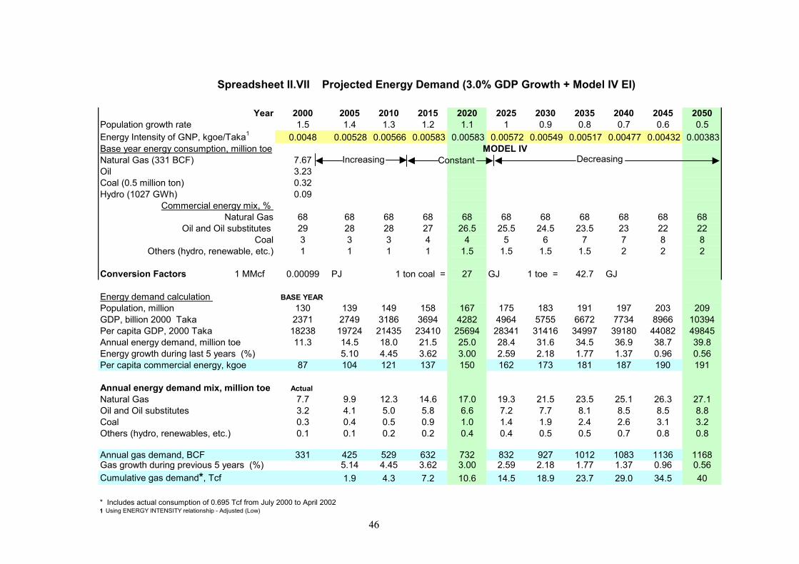
46

Spreadsheet II.VII Projected Energy Demand (3.0% GDP Growth + Model IV EI)

Year 2000 2005 2010 2015 2020 2025 2030 2035 2040 2045 2050Population growth rate 1.5 1.4 1.3 1.2 1.1 1 0.9 0.8 0.7 0.6 0.5Energy Intensity of GNP, kgoe/Taka1 0.0048 0.00528 0.00566 0.00583 0.00583 0.00572 0.00549 0.00517 0.00477 0.00432 0.00383Base year energy consumption, million toe MODEL IV Natural Gas (331 BCF) 7.67Oil 3.23Coal (0.5 million ton) 0.32Hydro (1027 GWh) 0.09


Oil and Oil substitutes 29 28 28 27 26.5 25.5 24.5 23.5 23 22 22Coal 3 3 3 4 4 5 6 7 7 8 8






* Includes actual consumption of 0.695 Tcf from July 2000 to April 2002 1 Using ENERGY INTENSITY relationship - Adjusted (Low)


Spreadsheet II.VIII Projected Energy Demand (4.55% GDP Growth + Model IV EI)



Oil and Oil substitutes 29 28 28 27 26.5 25.5 24.5 23.5 23 23.3 23.9Coal 3 3 3 4 4 5 6 7 7 6.7 6.1








47

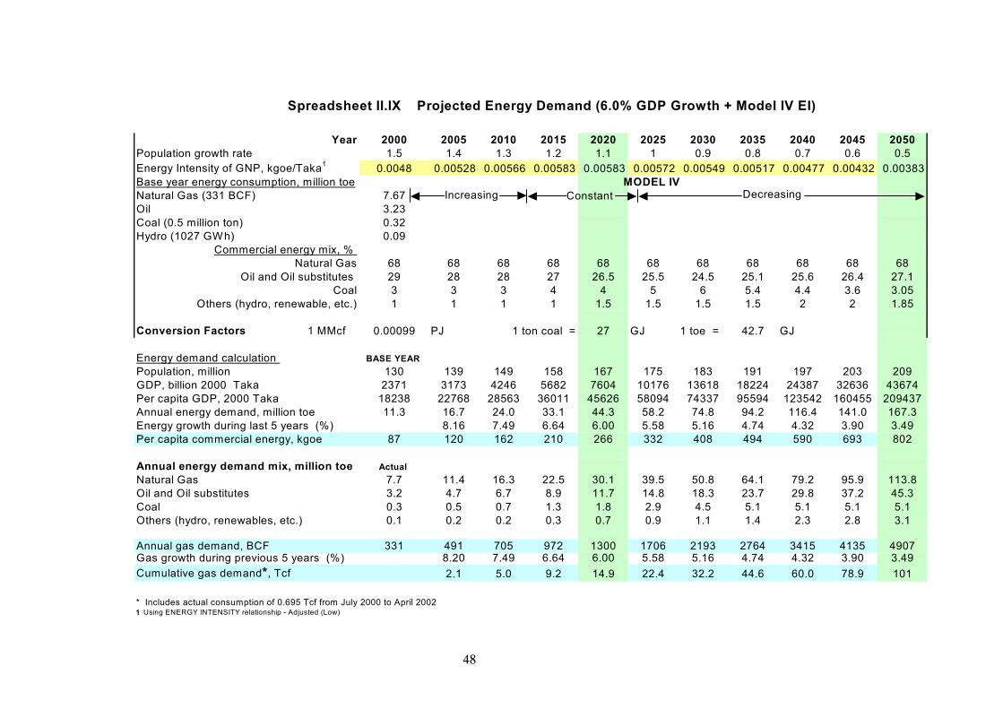
Spreadsheet II.IX Projected Energy Demand (6.0% GDP Growth + Model IV EI)



Oil and Oil substitutes 29 28 28 27 26.5 25.5 24.5 25.1 25.6 26.4 27.1Coal 3 3 3 4 4 5 6 5.4 4.4 3.6 3.05








48

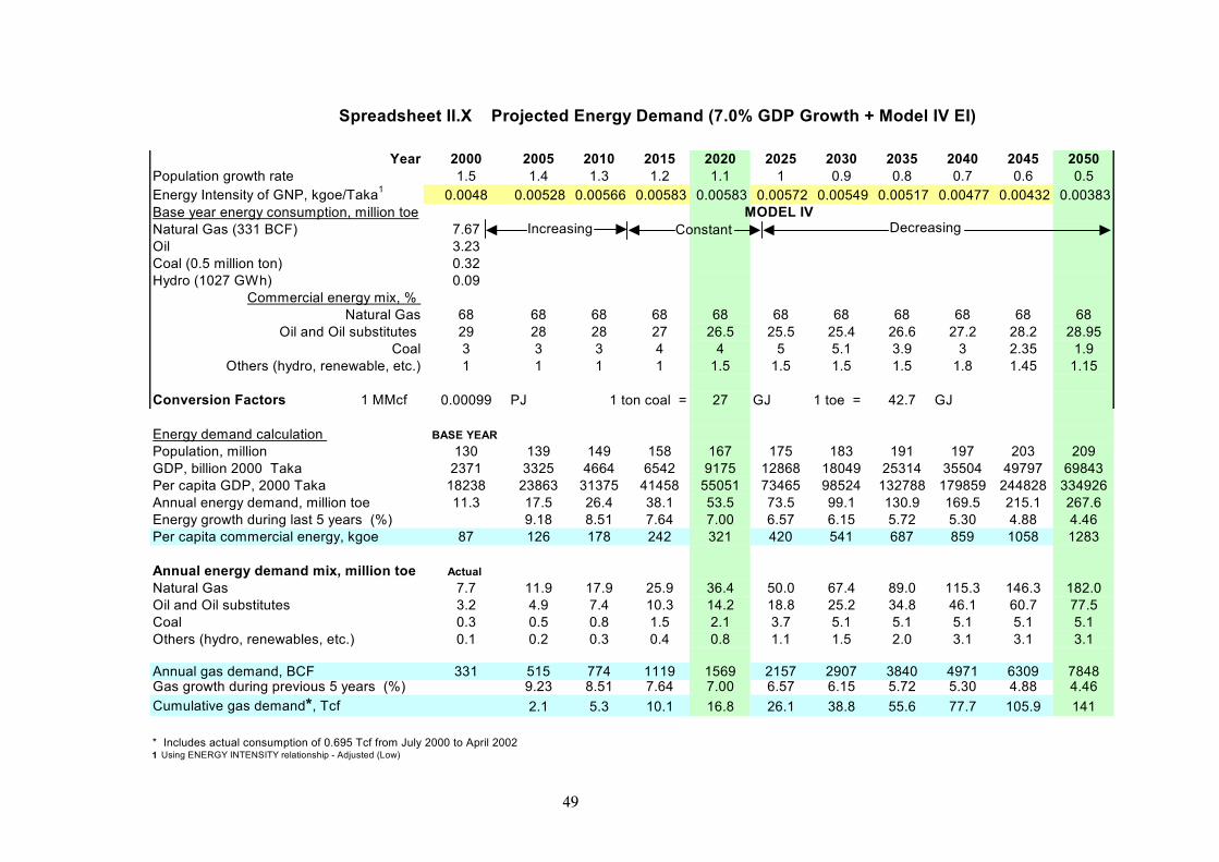
Spreadsheet II.X Projected Energy Demand (7.0% GDP Growth + Model IV EI)



Oil and Oil substitutes 29 28 28 27 26.5 25.5 25.4 26.6 27.2 28.2 28.95Coal 3 3 3 4 4 5 5.1 3.9 3 2.35 1.9

Others (hydro, renewable, etc.) 1 1 1 1 1.5 1.5 1.5 1.5 1.8 1.45 1.15







49

3. ASSESSMENT OF RECOVERABLE GAS RESERVE

50

3.1 Introduction

Gas is the most valuable natural resource of Bangladesh. Future development of the

country largely depends on judicious use of this valuable resource. In this chapter the

reserves of all the discovered gas fields have been updated based on previous study

reports and latest information of the fields. There has been a number of studies

conducted on the gas fields of Bangladesh starting from mid seventies. It is not an

easy task to review all the existing studies and come to a conclusion for the gas

reserve since these studies were conducted at different point of time following

different methodologies, criteria and using different set of data. The scope of re-

estimation using a uniform methodology for all the gas fields is beyond this

Committee. Only published results have been considered and the basis or rationales

behind the results have been examined. Within the time and resource limitation of this

Committee, maximum effort has been given to judge and analyse the works that are

available for review. Reserve estimation is a dynamic process and it needs to be

updated every year using additional pressure/production data and additional

information of the development/appraisal activities.

In this chapter reserve classification, review of past reports, and methodologies of

reserve estimates have been discussed briefly. Based on critical review and analysis of

the past studies/reports and latest information and data of the reservoir, reserve

estimates of all fields have been updated. Finally, some conclusions and

recommendations are made.

3.2 Review of Past Reports

A number of studies were conducted by various agencies/organisations in the past.

Some of them were for limited number of fields while the others were for

countrywide assessment. Bangladesh started producing gas on a commercial basis

since 1963. The early use was on a very limited basis. The total gas use until 1980

was about half a Tcf.

A number of foreign countries provided technical assistance in gas sector

development and assessing the gas reserve of the country. The then Soviet Union

51

(1964-75) provided technical assistance in geological and geophysical surveys and

exploration in different onshore areas of the country. The Federal Republic of

Germany (1976-86, 1995-96, 2000-To-date) provided technical assistance to

Petrobangla with geological and geophysical surveys, exploration, assessment of

hydrocarbon reserves and resources of the eastern and western parts of the country,

and human resource development. The United Kingdom (1979-86) also provided

assistance with geophysical and assessment of hydrocarbon reserves and resources

of the country.

Petroconsultant undertook the first significant effort for a gas inventory in the country

in 1979. After that, many other studies were conducted namely: Petrobangla (1981),

Degolyer & MacNaughton (1984), German Geological Advisory Group (GGAG,

1986), Hydrocarbon Habitat Study of Bangladesh (HHSB, 1986), Gasuine (1989),

Welldrill (1991), IKM (1991), Clyde Petroleum (1995), Nico/BAPEX (1997),

Petrobangla/Biecip-Franlab (2000) and Hydrocarbon Unit/Norwegian Petroleum

Directorate (HCU/NPD, 2001). Apart from these studies, the only other published

data on a reserve study was from the PMRE department, BUET (2001).

Most of the earlier studies severely suffered from lack of sufficient

production/pressure data and had to depend on the more uncertain volumetric

estimation. All of the above mentioned studies were reviewed in assessing the up to

date reserve of the country. Four gas fields under the PSC agreement with Shell and

UNOCAL were assessed differently. As each PSC has a dynamic process of

evaluating the fields where both Petrobangla and the IOC agree on a number at a

given time under the contract, fields under PSCs were not reviewed for reserves

update in the present study.

IKM (1991) studied eight gas fields (Titas, Bakhrabad, Kailashtilla, Habiganj,

Rashidpur, Beanibazar, Belabo and Meghna) and used different methods under

different field circumstances for reserve estimates and recovery calculation. These

included volumetric method using the isopach maps and material balance for reserve

estimate. Numerical simulation and material balance were used for recovery

calculation. The key parameter for all their decision making was the drive mechanism.

52

Water-drive or depletion-drive was considered case by case. Their recovery efficiency

was entirely dependent on the type of drive they assumed.

Welldrill (1991) reviewed seventeen gas fields (Titas, Bakhrabad, Kailashtilla, Habiganj,

Rashidpur, Beanibazar, Belabo, Meghna, Begumganj, Chattak, Fenchuganj, Feni, Jalalabad,

Kamta, Kutubdia, Semutang and Sylhet) at that time using a combination of volumetric and

material balance analyses. Like all other studies in the earlier period, they were limited by

lack of sufficient pressure-production data. Using a combination of volumetric and MB data,

they made a reasonable estimate. Both IKM and Welldrill studies were conducted about

twelve years ago. Since then significant pressure/ production data have become available. A

number of development/appraisal wells have also been drilled since then.

Nico/BAPEX (1997) conducted their study on three smaller fields. These are

Chatak, Feni and Kamta. These are one or two well fields where production was

suspended at different stages. At least two of these fields have strong indication of

engineering problem that are not related to the actual reserve or its recovery. Since

the study, Nico is trying to develop these reservoirs as marginal fields.

Under the reservoir management TA project, Reservoir Study Cell of Petrobangla

undertook an initiative to assess all the major producing fields with the help of

Beicip-Franlab Consultants (2001). This joint study completed their work on

Habiganj and Bakhrabad field and presented the report to the Petrobangla Board.

Both were very comprehensive studies analysing all aspects of reservoir

engineering. This project was supposed to study all the fields but due to funding

problem it was stopped in the middle of Titas field study. Because of that the two

complete field reports were presented as interim report.

HCU/NPD (2001) re-estimated four major gas fields (Rashidpur, Kailastila,

Habiganj and Titas) using volumetric and material balance methods (modified

classical and Hevlena-Odeh method). Along with the re-estimation of reserve, the

recovery factor was also adjusted based on reservoir performance. ‘GeoX’ software

was used for the volumetric estimate and MBAL for material balance. For the

remaining fields, old reports were reviewed and all recovery factors were adjusted

to 70%.

53

The PMRE (2001) study updated the reserves of all producing gas fields of

Bangladesh (including suspended ones). Flowing well material balance method was

used to do the estimate. A comparison of the volumetric estimates was also

presented. In absence of good shut-in pressure data, this method is well established

as a tool to estimate GIIP. In Alberta, Canada, this method is being used routinely

to estimate gas pool reserves.

3.3 Methodology of Reserve Estimates

Various methods are used to estimate the reserves of discovered reservoirs depending

on the availability of data and development stage of the reservoir. The methods that

are used predominantly are: Volumetric, Material Balance, Decline Curve, and

Reservoir Simulation. As all of these methods are associated with various degree of

uncertainties, most of the time more than one method is used to increase the accuracy

of the estimates.

Volumetric method: In volumetric method estimated rock volume of the reservoir is

multiplied with porosity and gas saturation to calculate the gas in place. Although the

calculation procedure is very simple, important consideration is the uncertainty

associated with the data used. Volumetric methods are used early in the life of the

reservoir before any significant production and development activities. Obviously

early in the production life of a reservoir when few data are available to establish the

subsurface geologic control, volumetric estimates are least accurate (Lee and

Wattenburger, 1996). Accuracy of volumetric estimates however increases with

production and development activities, as more data become available.

Material balance: Calculation of in-place volumes of hydrocarbons by material

balance requires equating the incremental expansion of the reservoir fluids upon

pressure drop to the reservoir voidage caused by the withdrawal of oil, gas and water,

corrected for any fluid influx or injection. It is generally accepted that methods based

on production performance data are more accurate than those based strictly on

inference from geological and engineering data. This conclusion is widely accepted in

literature and professional practices. Accuracy of material balance, a performance

based method, increases with production and pressure decline. Unlike the volumetric

54

method, the material balance accounts for reservoir heterogeneity and continuity

variations that occur away from the existing wellbore. In such instances, the accuracy

of reserve estimates is greatly improved through material balance analysis. Accuracy

of the volumetric estimates depends on quality of seismic and log data and is severely

affected by well density. Skill, experience and expertise also play a vital role on the

reliability of seismic interpretation. Similarly, lack of production/pressure data and

their reliability may affect the production performance based techniques. There are

several variations of the material balance method. These are: classical material

balance (CMB); modified classical material balance (MCMB); Hevlena and Odeh plot

(H-O); and flowing well material balance (FWMB). Based on specific situation and

available information one or more of these methods are applied.

Decline curve and Simulation: Among the production-based techniques, perhaps

production decline curve analysis would give the best GIIP value as this is applied to

the declining stage of the field production. Only a couple of fields have reached that

situation in Bangladesh and none of the studies considered this method. Numerical

simulation, specially the integrated reservoir simulation technique is also used for

estimating purpose. Numerical simulation is essentially a material balance method

applied to small cells of the reservoir and is used more for history matching and

predicting future production profile and/or recovery. While using numerical

simulation utmost importance should be given in establishing the correct reservoir

model to obtain meaningful results.

In the context of gas reserves, both volumetric and material balance methods are

extensively used depending on the various stages of development. Most of the

previous studies used volumetric and material balance methods to estimate the

reserves. Only IKM used simulation along with volumetric and material balance

methods. Since all methods are associated with certain degree of uncertainties, it is

standard industry practice to use several methods to reduce uncertainty and increase

the level of confidence in the estimates.

55

3.4 Reserve Classification

To improve the level of consistency in reserve estimation and reporting, the Society of

Petroleum Engineers (SPE) and the World Petroleum Congress (WPC) approved in

1997 a set of petroleum reserves definitions, which was supported by the American

Association of Petroleum Geologists (AAPG). Although these definitions are widely

referred, individual estimator’s judgement plays a big role in reserve classification.

Proved Reserves: Proved reserves (P1) are those quantities of natural gas, which by

analysis of geological and engineering data, can be estimated with reasonable

certainty to be commercially recoverable, from a given date forward, from known

reservoirs and under current economic conditions, operating methods, and

government regulations.

If deterministic methods are used, the term reasonable certainty is intended to

express a high degree of confidence that the quantities will be recovered. If

probabilistic methods are used, there should be at least a 90% probability that the

quantities actually recovered will equal or exceed the estimate. Proved reserves can

be categorised as developed or undeveloped.

Developed: Reserves that are recoverable from existing wells with current operating

methods and expenses. Developed reserves may be sub-categorised as producing or

non-producing.

Undeveloped: Reserves that are recoverable from additional wells yet to be drilled,

and/or where large expenditure is required among others to install production or

transportation facilities for primary or improved recovery projects.

Unproved Reserves: Unproved reserves are based on geologic and/or engineering

data similar to that used in estimates of proved reserves; but suffer from technical,

contractual, or regulatory uncertainties. The unproved reserves can be categorised

into probable and possible reserves.

56

Probable Reserves: Probable reserves (P2) are those unproved reserves which analysis of

geological and engineering data suggests are more likely than not to be recoverable. In this

context, when probabilistic methods are used, there should be at least a 50% probability that

the quantities actually recovered will equal or exceed the sum of estimated proved plus

probable reserves.

Possible Reserves: Possible reserves (P3) are those unproved reserves which

analysis of geological and engineering data suggests are less likely to be recoverable

than probable reserves. In this context, when probabilistic methods are used, there

should be at least a 10% probability that the quantities actually recovered will equal

or exceed the sum of estimated proved plus probable plus possible reserves.

Field Growth: Field growth means additional reserve potential of a field as a result

of applying new technology such as, 3D seismic, installing compression facilities

and applying better reservoir management techniques. Field growth reserve is

generally identified at a later stage of the reservoir life due to additional financial

incentives becoming available. As demonstrated in the Rashidpur gas field, 3D

seismic can identify thin beds, which can bring in additional gas reserve from an

existing field. In most of the gas fields of the country reserve is calculated assuming

1100 psi at the wellhead. Compression will allow reservoir pressure to fall further

than that normally required for the processing and high-pressure transmission lines,

and thus will enable further production from the reservoir. Better reservoir

management always means better recovery and additional production from the

reservoir. It is very difficult to quantify the total field growth potential of the

country at this early stage of development of its gas fields since no serious study has

been conducted in this regard. But considering the development stage of the gas

fields, it is axiomatic that the reserve of the discovered fields is going to increase in

future through field growth.

Limitations of SPE and WPC Definitions: The initial reserve of a field will be

known absolutely only on the day when the field is finally abandoned and the

reserve equates with the cumulative production. The SPE and WPC have

endeavoured, without much success, to find a compromise between the determinist

and probabilistic schools of thoughts. Their 1997 definition is a poor compromise and

is not strictly followed. The term “reasonable certainty”, which is used to define 57

proved status can mean anything with a probability of between 50% and 90%. Outside

the US, many companies prefer the probabilistic method, using P90, P50 and P10 to

generate a mean or expected value. UK accounting procedure requires to be defined

as Proved + Probable (2P), which is normally taken at a P50 value. All over the

world, an overwhelming majority of the organisations use the 2P for internal planning

purpose. On many occasions political and/or economic factors play a vital role behind

reporting a certain reserve figure, that has no bearing on the development-supply

planning of fields. Vast majority of the world reserve estimates use deterministic

approach where the ‘reasonable certainty’ for proved reserve solely depends on the

experience and judgement of the estimator.

3.5 Recovery Calculation

Recovery Efficiency (RE) depends mainly on the reservoir characteristics and drive

mechanism. Experience with volumetric gas reservoirs indicates that the recoveries

range from 80 to 90 percent (Crafts and Hawkins, 1991, Lee and Wattenberger,

1996). Gas reservoirs with active water drive may have recovery factor of 50 to 85

percent. These two being the worst and best case scenarios with most likely value of

around 70%. The true RE will depend on the reservoir condition and the influx rate

(aquifer strength) and pattern. The true recovery factor may be calculated from

residual gas saturation in the water invaded zone and the recommended method of

determining residual gas saturation is measurement from representative core samples

or from the actual inventory of the gas (Crafts and Hawkins, 1991). The best way to

estimate recovery is from well performance and reservoir simulation that should be

dynamically done with close well performance monitoring.

With the life of a field, recovery factor increases most of the time because of poor

estimate at the beginning, when using proper estimates, recovery factor does not

change too much with time (Laherrere, 1997). The first task for calculating

recovery factor is to identify the drive mechanism. In early stage of the production,

when the influence of water influx is difficult to identify, geologic and engineering

data are consulted to establish the drive mechanism. Once the field has produced

more than 10% of its GIIP, material balance may clearly indicate the drive

mechanism. Like any other mathematical model this also have exceptions.

58

The reservoir management is the most important issue that needs to be considered

for the ultimate RE estimation. Improper development plan, non-optimised

production ignoring drive mechanism and/or reservoir structure may damage the

reservoir. This could also occur due to wrong, inadequate or lack of engineering

intervention and delay in any remedial step. As a result, best recovery may not be

achieved leaving a large amount of resource under ground.

IKM used both material balance and numerical simulation to estimate the recovery.

Petrobangla/Biecip-Franlab and HCU/NPD studies tried to establish the drive

mechanism and based on that assumed the recovery factors. Welldrill study did

some limited analysis and suggested recovery factors reviewing all the reports

available at that time. In this study reservoir drive mechanism and results of

previous studies have been considered in estimating the recovery factors.

3.6 Estimation of Reserves

The Committee reviewed all the available studies/reports and latest information and

has come up with two estimates of the gas initially in place (GIIP) and recoverable

reserves of all the gas fields. The two estimates are identified as Estimate 1 and

Estimate 2, detail of which will be provided in Volume 2 of this report.

Following are the criteria for Estimate 1:

• No re-calculation/re-estimation was done

• Updating was done based on published data only that were made available to the

Committee

• First priority was given to appropriate MB results if the cumulative production

were at least 10% of the gas in place of the reservoir. Up to date

pressure/production data, drive mechanism and production history were

considered in accepting or rejecting any results

• Last (latest) volumetric estimate was used in absence of reliable/adequate/any

production-pressure data

59

• Combination of volumetric and MB results were used in case of inadequate

geologic control and pressure-production data

• For non-producing, suspended and PSC fields, official Petrobangla estimates were

used

Factors considered to estimate recovery efficiency are as follows:

• Drive mechanism

• Reservoir characteristics

• Reservoir management

For depletion type reservoirs and situations where sufficient production data are

available, recovery factors are estimated from the flowing material balance results

(PMRE, 2001).

Estimate 2 includes re-estimation of GIIP of the four major gas fields (Titas,

Kailashtila, Rashidpur and Habiganj) using the volumetric method. Predominant

criterion for this estimate was to consider mainly the volumetric results of previous

studies. Recovery efficiency estimation was mostly assumptions.

Results of the two estimates are provided in Table 3.1 and 3.2.

60

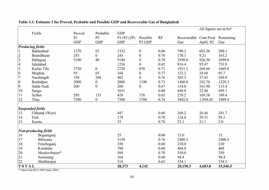
Table 3.1: Estimate 1 for Proved, Probable and Possible GIIP and Recoverable Gas of Bangladesh

All figures are in bcfFields Proved Probable GIIP

P1 P2 P1+P2 (2P) Possible RF Recoverable Cum Prod Remaining GIIP GIIP GIIP P3 GIIP Gas April, '02 Gas Producing fields 1 Bakhrabad 1270 62 1332 0 0.60 799.2 603.20 200.12 BeaniBazar 243 0 243 0 0.70 170.1 9.21 163.23 Habiganj 5100 40 5140 0 0.70 3598.0 926.30 2699.04 Jalalabad 1256 0 0.65 816.4 92.47 733.95 Kailas Tila 2720 0 2720 870 0.71 1931.2 268.60 1669.86 Meghna 95 65 160 0 0.77 123.2 28.60 95.77 Narshingdi 194 208 402 0 0.76 305.5 37.43 269.98 Rashidpur 2000 0 2000 1190 0.73 1460.0 242.76 1229.39 Salda Nadi 200 0 200 0 0.67 134.0 161.90 113.410 Sangu 1051 0.80 840.8 22.40 695.711 Sylhet 295 133 428 376 0.65 278.2 169.38 109.412 Titas 7300 0 7300 1700 0.74 5402.0 1,954.45 3489.4

Suspended fields 13 Chhatak (West) 447 0.60 268.2 26.46 241.714 Feni 178 0.70 124.6 39.51 85.115 Kamta 33 0.70 23.1 21.1 2.0

Non-producing fields 16 Begumganj 25 0.60 15.0 1517 Bibiyana 3150 0.76 2400.3 2400.318 Fenchuganj 350 0.60 210.0 21019 Kutubdia 780 0.60 468.0 46820 Moulovibazar* 500 0.70 350.0 35021 Semutang 164 0.60 98.4 98.422 Shahbazpur 514 0.65 334.1 334.1T 0 T A L 28,373 4,142 20,150.3 4,603.8 15,546.5

* Taken from HCU-NPD Study (2001)

61

Table 3.2: Estimate 2 for Proved, Probable and Possible GIIP and Recoverable gas of Bangladesh All figures are in bcf

Fields Proved Probable GIIP P1 P2 P1+P2 (2P) Possible RF Recoverable Cum Prod Remaining GIIP GIIP GIIP P3 GIIP Gas April, '02 Gas Producing fields 1 Bakhrabad 1,369.70 62.30 1432 0 0.61 873.52 603.20 270.322 BeaniBazar 243.10 0 243.1 0 0.65 158.02 9.21 148.813 Habiganj 3,501.66 0 3501.66 0 0.52 1,820.86 926.30 894.564 Jalalabad 1,015.31 179.36 1194.67 299.26 0.55(.71*) 685.77 92.47 593.35 Kailas Tila 1,722.08 0 1722.08 1,780.0 0.69 1,188.24 268.60 919.646 Meghna 76.00 83.00 159 128.00 0.65 103.35 28.60 74.757 Narshingdi 64.80 46.00 110.8 84.00 0.65 72.02 37.43 34.598 Rashidpur 1,304.25 697.75 2002 2,948.00 0.58 1161.17 242.76 918.419 Salda Nadi 134.78 244.81 379.59 0 0.65 246.74 22.40 224.3410 Sangu 592.00 439.00 1031 0 0.82 845.42 161.90 683.5211 Sylhet 383.02 60.98 444 0 0.65 288.6 169.38 119.2212 Titas 4,045.64 3,247.11 7292.75 2100.0 0.65 4740.29 1,954.45 2785.84

Suspended fields 13 Chhatak (West) 265.00 209.00 474 728.00 0.60 284.0 26.46 257.5414 Feni 66.00 105.00 171 207.00 0.60 102.6 39.51 63.0915 Kamta 38.00 0 38 36.00 0.60 22.8 21.1 1.7

Non-producing fields 16 Begumganj 14.00 32.60 46.6 107.70 0.65 30.29 30.2917 Bibiyana 1,583.65 1,560.87 3144.52 3,422.66 0.76 2389.84 2389.8418 Fenchuganj 85.00 319.00 404 0 0.65 262.6 262.619 Kutubdia 61.00 800.00 861 0 0.65 559.65 559.6520 Moulovibazar* 500 0.70 350.0 35021 Semutang 24.50 149.70 174.2 0 0.65 113.23 113.2322 Shahbazpur 306.60 207.20 513.8 0 0.65 334 334T 0 T A L 16,896.09 8,443.68 25,839.77 11,840.62 16,644.31 4,603.77 12,040.54

* Taken from HCU-NPD Study (2001)

62

Table 3.1 of Estimate 1 shows proved + probable (2P) GIIP and recoverable reserve as

28.37 Tcf and 20.15 Tcf, respectively. In April 2002, cumulative production stood at 4.60

Tcf. Therefore, the remaining reserve of the country is 15.55 Tcf. Estimate 1 also shows

a possible GIIP (P3) of 4.14 Tcf of gas.

Table 3.2 of Estimate 2 shows proved + probable (2P) GIIP and recoverable reserve as

25.84 Tcf and 16.64 Tcf, respectively Therefore, according to this estimate the remaining

reserve of the country is 12.04 Tcf as of April 2002. Estimate 2 however shows a possible

GIIP (P3) of 11.84 Tcf which is significantly higher than that of the Estimate 1.

Therefore, after reviewing the results of the two estimates, the Committee concludes that

the remaining recoverable proved + probable reserve (2P) of the country ranges between

12.04 Tcf and 15.55 Tcf. With regular reserve updates and additional information,

accuracy of reserve estimates is going to improve in the years to come.

3.7 Conclusions

1. Due to inadequate drilling and appraisal/development activities, reserve estimates of

Bangladesh have lot of uncertainties. A intensive drilling and appraisal program should be

undertaken to reduce these uncertainties.

2. Reserve estimation is a dynamic process and estimated results are always associated with

certain degree of uncertainties until the reservoir is fully depleted. As more and more data

and information become available with time, the uncertainty decreases with updated

reserve estimates.

3. At the beginning of the reservoir development and production, reserves are estimated

based on geological and engineering data having higher degree of uncertainty associated

with the estimates. However, at later stages, production data and additional well

information from appraisal/development drilling are given more emphasis in estimating

the reserves.

63

4. Recovery from gas reservoirs depends primarily on the nature of the reservoir, reservoir

drive mechanism, reservoir characterisation, reservoir heterogeneity, well locations, well

completions, reservoir depletion and reservoir management strategy.

5. After reviewing the available reports the Committee estimates the remaining recoverable

proved + probable reserve (2P) of the country to be in the range of 12.04 Tcf to 15.55

Tcf. The Committee also estimates the possible GIIP (P3) of the country to be in the

range of 4.14 Tcf to 11.84 Tcf.

3.8 Recommendations

Although Bangladesh is producing natural gas for over three decades all of its major gas

fields are underdeveloped and have not been properly delineated yet. Reserve estimation

is a dynamic process and all the estimation processes are associated with certain degree of

uncertainties. Therefore, a systematic and sustained approach should be taken by the

concerned organisations and agencies to develop all the gas fields of the country. The

reserve of each field should be updated once a year during the producing life of the field.

Additional seismic and appraisal/development activities should be undertaken to reduce

the high uncertainties of the country’s reserve estimate.

3.9 References

• Laherrere, J. (1997) : “Distribution and evolution of recovery factor”, Oil reserve conference, Nov. 11, USA.

• Lee and Wattenbarger (1996): “ Gas Reservoir Engineering” Published by the Society of Petroleum Engineers, Richardson, TX.

• Crafts and Hawkins (1991): “Applied Reservoir Engineering”, 2nd Edition, Prentice Hall Publishing Company, USA.

• Dake (1997): “The Practice of Reservoir Engineering” Elsevier Science, B.V., Netherlands.

• IKM (1991): Gas Field Appraisal Project, Geological, Geophysical, Petrophysical and Reservoir Engineering Reports, Petrobangla.

• Welldrill (UK) Ltd. (1991): “Review of Gas Reserves in Bangladesh for Petrobangla”, Petrobangla.

64

• Beicip-Franlab-Petrobangla (2000): “Interim Report on Hydrocarbon resources for Enhanced Reservoir (ASSET) Management” Petrobangla.

• HCU-NPD (2001): “Bangladesh Petroleum Potential and Resource Assessment 2001” , HCU, Ministry of Energy and Mineral Resources, GOB.

• PMRE (2001): “Estimation of Gas In Place of Bangladesh Using Flowing Material Balance Method” A paper by B. HOQ and E. Gomes presented at the 4th International Conference on Mechanical Engineering, BUET, December.

65

4. GAS RESOURCE ASSESSMENT

66

4.1 Introduction

The objective of this report is to provide an updated, reliable and scientific estimate of the

country's undiscovered gas resource potential by reviewing and evaluating various studies

conducted to date regarding hydrocarbon resources. Such an objective assessment has been

considered essential to support the national planners for gas exploration and utilization as a

number of studies provide widely varying results thus creating a lot of confusion amongst the

people. The most significant aspect that has been fuelling the confusion is the frequent use of the

terminology of gas reserves to mean undiscovered gas resources, or amalgamating the two

categories of resources. This chapter, therefore, only addresses the undiscovered gas resource

potentials and not the discovered gas resources (i.e. reserves), which have been treated in a

separate chapter by the Committee.

Gas was first discovered in the country in 1956 and production started in 1962. Since then

exploration activity was continuing in the country resulting in the discovery of 22 gas fields and 1

oil field. In fact, exploration for oil in the geologic area of today's Bangladesh started as early as

1908 by the India Petroleum Prospecting Company; which was continued by many other

companies and the State enterprises with occasional breaks resulting in improved understanding of

the regional geology from the geophysical acquisitions, drilling, logs and production data. As is

obvious many resource assessment studies have been conducted in the process to integrate these

information with newer tools and methodologies by various study groups/ explorationists. The

more representative of such reports cover the period of 1986 to 2001 which could be considered

by the Committee for its technical review and evaluation.

Natural gas is the main commercial energy in the county. This study update covers review, of the

geological development, and assessments of various methodologies and results of previous study

groups or consultants and recommends a set of results of undiscovered gas resource result that

could be used for exploration of this vital resource until these results are further updated with new

data.

67

4.2 Regional Geological Setting and Tectonic Evolution

The geology of Bangladesh may be traced back in time to the latest Paleozoic (350 million years

ago) when the ancient continent of Pangea broke apart and fragments of the earth’s crust began to

migrate northward toward an ultimate collision with the southern portion of Asia. One of these

lithospheric fragments, the Indian subcontinent, continued to drift throughout almost all of the

Mesozoic and into the early Cenozoic before early collision with southern Asia closed the ancient

ocean on the north of the Indian subcontinent and drove up the Himalaya Mountain chain. At the

same time, collision, subduction, and compressional forces formed the mountainous regions in

Myanmar to the east and produced the geoanticlinorium of the Arakan Yoma in adjacent Myanmar

and eastern India. These recently uplifted highlands to the north and east, as well as the ancient

land mass of India on the west, were subsequently eroded and shed sediment into the deep basin to

the east, south, and west, into the area currently underlying the great Ganges-Brahmaputra delta.

The sediments of the Ganges-Brahmaputra delta underlie almost all of Bangladesh, parts of eastern

India, and West Bengal. Total sedimentary thickness in Bangladesh is unknown, but probably

exceeds 20,000 meters in the area of the Surma Basin and in the southern part of the Ganges-

Brahmaputra delta. This thick pile of sediments overlies the deeply buried crust of the ancient

Indian subcontinent on the west and now deeply buried oceanic crust on the east and there is a

distinct geological difference between the eastern and western part of the country. On the east,

were the oceanic crust beneath the delta is being subducted into the earth beneath the Burma plate,

the overlying sediments are being scraped off into a series of elongate, and gentle to complexly

faulted folds (fig.4.1).

4.3 Petroleum System and Assessment Units

For undiscovered Gas Resource Assessment, the Petroleum System of a region or country needs to

be studied throughly. The information on Petroleum system is used to identify and describe Total

Petroleum Systems (TPS) within the assessed region. As far as possible, Total Petroleum Systems

encompass the natural process that begins with the Generation of hydrocarbon from kerogen-rich

source rocks, is followed by the migration of hydrocarbons from their soorce area, and ends with

68

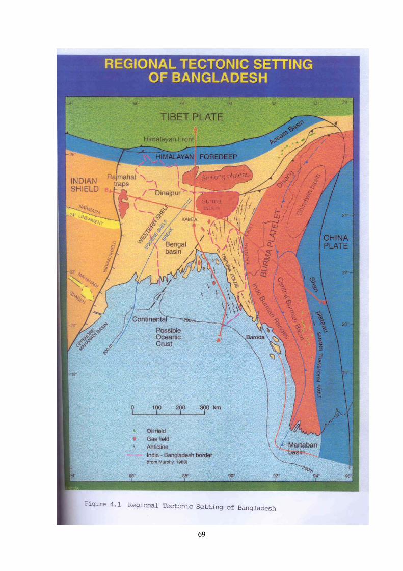
69

their entrapment within reservoir rocks beneath relatively impervious seals. The area (or country)

in which that total Petroleum System is active is then divided into Assessment Uints (AU) .

In USGS/ Petrobangla Gas Resource Assessment study the Total Petroleum System with system

elements like: Source Rock, Migration, Reservoir Rock, Seal and Trap within the great Tertiary

delta is treated as a single composite Total Petroleum System (TPS). The nomenclature, coding

system such as BANG 01 Tertiary Composite Total Petroleum System and supporting analytical

database follows procedures formally described in the USGS world Petroleum 2000 (U.S

Geological Survey World Energy Assessment Team 2000).

The USGS/ Petrobangla Gas Assessment team divided the country into six assessment units, based

to a large degree their geological structural attributes (fig.4.2).

These are : Bang 0101 Surma Basin Assessment Unit; This unit is a geophysically and

geologically defined area in the northeastern Bangladesh that contains a great thickness of tertiary

sedimentary strata. This AU is classified as a frontier area with a good umber of discovered Gas

fields that exceeded the minimum assessed size of 42 BCFG.

The Surma Basin Assessment Unit is a Potential source rocks include the shales and carbonaceous

shales of Eocene, Oligocene, and Miocene age. The strata generally contain about 0.5 to 3 percent

total organic carbon (TOC) although in places the content to organic matter may range up to 10.5

percent. Thermal maturation is sufficient to generate natural gas and natural gas liquids throughout

much of the area. Gas and condensates were generated at maturities equivalent to 1.1 to 1.3%

vitrinite reflectance (Ro) and at depths that range from about 6 to 7.5 km. Hydrocarbon generation

commenced a few tens of millions of years ago and has continued during the formation of the

major anticlinal traps, which began forming only several million year ago. Reservoir rocks in the

Surma Basin are chiefly tertiary age sandstones of the Boka Bil and Bhuban Formations (Miocene)

that were deposited in fluvial, deltaic and estuarine environments. Porosity ranges generally from

10 to 20 percent. Reservoir sands range from thick channel-fill and littoral or marine bar deposits

70

Figure-4.2 Estimates of Undiscovered Natural Gas Resources of Bangladesh

71

to sandstones thinly interlaminated with shale and siltstone that were deposited in tidally

influenced environments.

Structural and combination traps of Miocene age occur along stratigraphic boundaries, in

sandstone-filled channel deposits, and in sandstone beds sealed laterally by shale-filled channels,

and these comprise major traps in the eastern part of the basin. In general, these sedimentary

strata have been folded into several large scale anticlines that are unfolded or slightly to

moderately faulted in the western and central parts of the basin. Folding and faulting is intense

toward the east within the Chittagong-Tripura foldbelt, and becomes progressively less intense to

the west, where the folds are more broad and gentle. Major field discoveries in this AU include

Jalalabad Beanibazar, Chhatak, Sylhet, Moulavibazar, Rshidpur, Fenchuganj, Bibiyana, Kailshtila

and Habiganj.

Bang 0102 Eastern Extremely Folded Assessment Unit; This assessment unit is classified as

hypothetical because hydrocarbon in amounts exceeding the minimum field size have not been

found within it. This AU comprises the easternmost and most tectonically deformed AU in

Bangladesh. It consists of at least ten major anticlinal structures that being strata as old as Miocene

to the surface on their crests. The tertiary age stratigraphic units mapped in the tightly folded

anticlinal structures in the area (Alam and others, 1990) are the same as those recognized in the

subsurface of the Surma Basin. As a result of the intense folding and faulting, the source rocks

and reservoir rocks of the Surma Basin are exposed at the surface in this area where the anticlines

are breached by erosion. The few wells that have been drilled in this area tested the upper part of

the Surma Group, and all were plugged and abandoned. The Patiya well near Rangamati, drilled

into the Miocene in 1953 by Pakistan Petroleum Limited, encountered a show of oil in Miocene

strata.

Bang 0103 High amplitude Faulted Anticlines Assessment Unit; The Assessment Unit classified

as frontier because it has only one field that exceeds the minimum size of 42 BCFG. The High

Amplitude Faulted Anticlines Assessment Unit occupies the area east of the Moderately Faulted

Anticlines Assessment Unit and west of the Easternmost Extremely Faulted Assessment Unit in

easternmost Bangladesh.

72

It consists of at least seven major anticlinal structures that bring strata as old as Miocene up to the

surface in their cores. The Tertiary age stratigraphic units mapped in the tightly folded anticlinal

structures in this area (Alam and others, 1990) are the same as those recognized in the subsurface

of the Surma Basin. As a result of the intense folding the faulting, however, the source rocks and

reservoir rocks correlative to those in the Surma Basin are exposed at the surface in this area

where the anticlines are breached by crosion. Semutang Field the only field discovered in this

area, by the Pakistan Oil and Gas Development Corporation, and it is not producing.

This assessment unit was separated from Bang 0102 because it is not as greatly deformed

structurally, and contains a discovered gas field. In general the petroleum geology of the two

regions is much the same.

Bang 0104 Moderately Folded Anticlines Assessment Unit; The assessment unit is classified as

frontier unit because it has only nine fields that exceed the minimum size of 42 BCFG. The Bengal

foredeep, the large area generally to the south of the Surma Basin, is in the more distal region of

the thick Tertiary deltaic deposits of the Ganges-Brahmaputra delta. Overall, the sediments of the

AU are as thick as 20,000m in the Patuakhali depression, a depocenter located in the southeastern

side of the delta (Shamsuddin and Abdullah. 1997; Ganguly, 1997). Like Bang 0102 and Bang

0103 the Tertiary and Quaternary strata in this AU are deformed into a series of plunging folds

because of subduction beneath the Arakan Yoma geoanticlinorium to the east. In this AU

anticlinal structures range from tightly folded elongate and faulted structures on the east to broad

open relatively unfaulted structures on the west.

Although the source rocks in this area have not been identified with certainty they probably

contain woody organic matter in shale, shaly coal beds and coal from deeper Miocene and

Oligocene source rocks. The stratigraphic positions of the source beds are uncertain and the

hydrocarbons may be generated from relatively low concentrations of organic matter distributed

throughout a large volume of sediments. In addition, there is some evidence of potential marine

source rocks and more deeply buried Oligocene source rocks beneath the depths currently imaged

on seismic reflection data. Potential source rocks from Oligocene to mid-Miocene age are within

or have passed through the main gas-generating window prior to and during the development of

the major anticlines.

73

The low concentration of liquid hydrocarbons in fields from the southern limit of the Surma Basin

to offshore southeastern Bangladesh demonstrates that source rocks, wherever they are, are at an

appropriate level of thermal maturation to have generated large amounts of natural gas. Migration

pathways are complex and are generally vertical along faults and fractures and via gas chimneys,

and lateral through porous sandstones. Overpressured zones at depth may be a control on

migration and may impact on seal integrity, Such zones are believed to have significant future

potential for gas resources in Bangladesh. Future discoveries are expected within this

Overpressured zone, roll-over anticlines in extensional down-to-the basin structures and in a great

variety of stratigraphic and combination traps, many nearby existing known structures. Reservoir

rocks are in deltaic, littoral, and marine sandstones in the upper part of Mega Sequence MS 1, and

in the sandstone channel-fill deposits of MS-2. Porosity ranges generally from 10 to 25 percent.

Evidence from onshore sections to the east indicate that some of these tertiary strata may have

been deposited as turbidities in relatively deep water (Petrobangla and USGS Joint Resource

Assessment Team, “U.S. Geological Survey –Petrobangla Cooperative Assessment of

Undiscovered Natural Gas Resources of Bangladesh,” January 2001).

Major discoveries in this assessment unit include the following fields Titas, Bakhrabad, Megna,

Narsingdi, Shaldanadi, Kamta, Feni, Shahbazpur, Kutubdia and Sangu.

Bang 0105 Western Slope Assessment Unit; The Western Slope Assessment Unit occupies the

region between the Moderately Faulted Anticlines Assessment Unit on the east and the Western

Platform Assessment Unit on the west. It is classified as hypothetical because no gas fields larger

than 42 BCFG have been found in this sparsely explored area. Tectonically, the region is

generally unfolded and the major structures appear to be extensional rather than compressional.

The Tertiary strata of the assessment unit apparently overlie extended and thinned (transitional)

continental crust in the northern part of the AU and oceanic crust in near shore and offshore

regions to the south. The possibility of deep marine sediments, submarine fans, at the base of

74

prograding clonoforms seaward of a paleo-hinge line were also considered in this AU.

This AU has not been deformed in compression by the processes of crustal subduction that has

deformed easternmost Bangladesh. Major compressional structures are absent, and expected

structural traps will be related to extensional deformation, where listric down-to-the basin faults

have resulted in the formation of roll-over anticlines. These extensional faults may provide vertical

migration pathways for hydrocarbons that matured in more deeply buried source rocks.

Stratigraphic traps are anticipated to be abundant, and charging with hydrocarbons is expected to

have occurred early in the depositional history of this part of the basin as potential source rocks

and porous reservoirs were buried ever more deeply within the sedimentary basin. Thus far, this

large region of the delta has been little explored and no discoveries have been made therein.

Bang 0106 Western Platform Assessment Unit; This assessment unit is classified as hypothetical

since no fields have been found that exceed the minimum field size of 42 BCFG. In northwestern

Bangladesh, the Western Platform Assessment unit, consists of several buried regional geologic

structures. These structures are the eastward inclined Bogra shelf of early Tertiary age that is

terminated on the east by a paleo-hinge line, a buried structural saddle adjacent to the Shillong

Plateau, and a small area in northwesternmost Bangladesh that dips northwest into the Himalayan

foredeep. This area was assessed collectively as the Western Platform Assessment Unit.

Collectively the Mesozoic and Cenozoic strata in this area are about 5 to 7 km thick and consist

both of pre-collisional sequences that were deposited prior to and during the northward drift of

the Indian subcontinent, and the post collisional sequences that were deposited in mid to late

Tertiary time.

These strata have been drilled in numerous places in West Bengal, India and in a few places in

western Bangladesh. Although prospects and leads have been identified along unconformities, in

porous limestones and along extensional structures, only a few shows of hydrocarbons have been

discovered thus far. The most prospective areas of this assessment unit may be along the shelf

edge where hydrocarbons generated in the adjacent deep basin have migrated upward into traps to

the west.

75

The Western Platform Assessment Unit is underlain at depth by a Permian cost petroleum system,

which may contain coalbed gas in continuous accumulations within extensional Gondwana basins.

This petroleum system was not assessed in this study.

In Hydrocarbon Unit and Norwegian Petroleum Directorate (HCU/NPD) Resource Assessment

2001, the Country have been divided into 2 Petroleum province such as: Eastern Foldedbelt

Petroleum Province and Western Petroleum Province. Eastern Foldedlbelt Petroleum Province

again sub divided into 3 Petroleum Systems namely : Surma Petroleum System, Eastern Delta-

Hill tract Petroleum System, Southeastern Offshore Petroleum System. Similarly the Western

Petroleum Province have been subdivided into 3 Petroleum system namely: Gondwana Petroleum

System, Bogra Shelf Petroleum System and Western Delta Petroleum System (fig.4.3).

The Surma Petroleum System; is a northern Oligocence-Mioceene system, comprises the Surma

Trough and parts of the Eastern Foldbelt north of the Tangail-Tripura high. The system is

characterized by anticlinal traps with channel cuts created within Middle- to Late Miocene

reservoir sandstones. The play types of this petroleum system include anticlinal and a combination

of structural and stratigraphical traps that are already proved by drilling. In addition there are lots

of potential stratigraphic traps that are yet to be drilled. The hydrocarbon source of the system is

most likely the Middle Oligocene Jenam Shales, which have generated both gas and liquid

hydrocarbons. Additional source rocks may be the Bhuban- Bokabil Shales, deposited during

Early to Middle Miocene. About 80% of country’s discovered hydrocarbon resources are

currently found in this system. Only the anticlinal play has so far been drilled, and stratigraphical

and deeper plays are yet to be tested, which may contain significant hydrocarbon resource,-

including oil.

The Eastern Delta-Hill Tract Petroleum System; is the southern Miocence-Pliocene petroleum

system which includes the Hatia Trough and the Eastern Foldbelt south of the Tangail- Tripura

High , and extends into the offshore are to the south. Like the area to the north, this system is also

characterized by anticlinal trapping with intensive channeling and deep-seated faults. The

possibilities of stratigraphic traps are also high. The anticlines become steeper eastwards as a

result of the more intense folding.

76

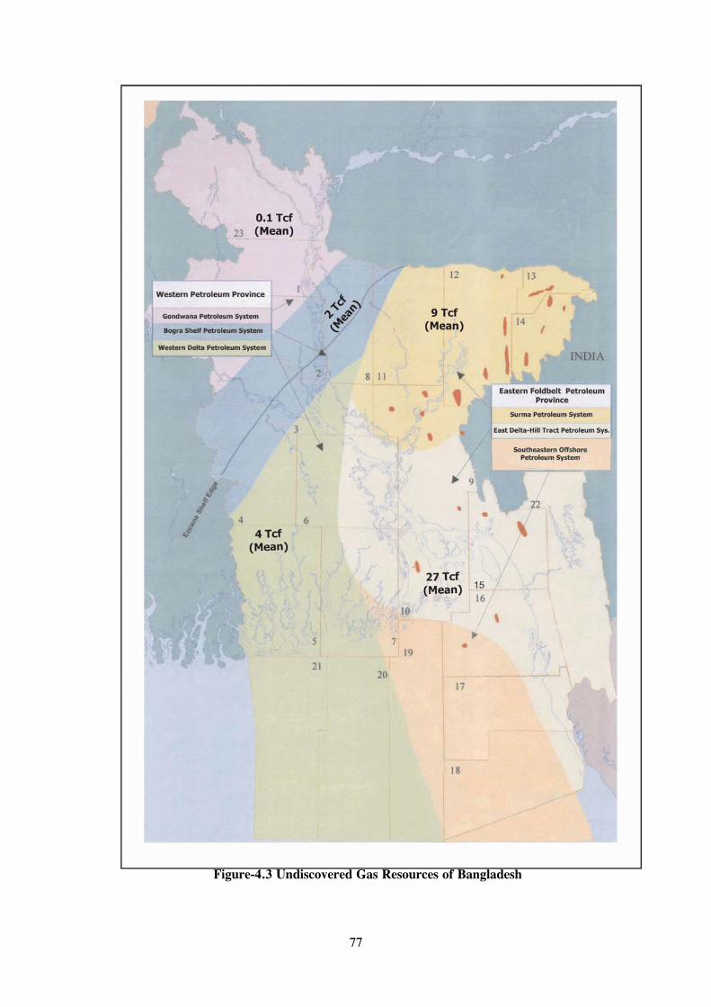
Figure-4.3 Undiscovered Gas Resources of Bangladesh

77

The reservoirs are Late Miocene to Pliocene sandstones deposited within fluvial distributary

channels and Miocene transgressive barrier bar sandstones. Seals are silty shales and mudstones,

and are developed locally within the Mio-Pliocene succession. Most likely the source rock is the

Miocene Bhuban Shales, found within the gas window, generating gas with a minimum of

condensate. Migration occurs mainly vertically, and is associated with deep-seated faults.

Accumulation of shallow, biogenic gas, along with thermogenic gas can also be observed in this

petroleum system. The area is relatively well explored. A recent discovery of gas in the

overpressure zone opens up a new potential of undiscovered resources of the entire country.

The Southeastern Offshore Petroleum System; a transition-like zone offshore, where the

southernmost petroleum system of each petroleum province merge. This will be overlying the East

Delta-Hill Tract Petroleum System, and comprises a stacked sedimentary succession of deposits

sourced both from the north as well as the east. The reservoir rocks will most likely be (Middle)/

Late Miocene-Pliocene delta front dominated sandstone bodies, turbidities and slope fan

complexes, but also large up-thrown and down-thrown growth fault traps. These stratigraphic

traps are sealed by interfingering, stacked shales, sourced by Late Miocene-Pliocene marine

deposits. Given the high sedimentation rates for the delta and slope fan complexes, these traps

must be regarded as important contributors to the resource base of Bangladesh. The Southeastern

Offshore Petroleum System is completely under-explored and needs further massive exploration.

So far no exploratory wells have yet been drilled in this system. The risk is regarded moderate.

Analogous deltaic systems around the world are regarded as very good petroleum systems.

The Gondwana Petroleum System; is restricted to the northwestern part of Bangladesh The

system is characterized by a passive margin setting within which the stratigraphic build-up took

place, creating potential traps ranging in age from Carboniferous through Late Cretaceous. The

succession comprises both sediments and volcanic rocks, providing all elements of a petroleum

system. The system has proved source rocks within the coal-bearing sequences. However, the

system is currently under-explored in Bangladesh and yet to be proved. The major play types of

78

this system are related to grabens and tilted fault blocks. As generation and migration of gases

from the Gondwana coals continue today, the Gondwana coals might also charge any trap within

the Paleogene -Neogene sediments above. The Gondwana Petroleum system must be regarded as a

high-risk system.

The Bogra Shelf Petroleum System; includes parts of the western shelf and the slope area of the

Bengal Foredeep. The system is characterized by a passive margin setting, underlain by a

continental basement within an extensional tectonic regime. The deposition took place from Late

Cretaceous through Late Eocene, with classic as well as carbonate sedimentation. Varieties of play

types like roll-over anticlines, Eocene carbonate build-ups, and unconformity related types traps as

well as late lowstand deposits and early transgressive sand bodies of the Oligocene close the shelf

slope break, could be the major exploration targets of this system. The Paleocene Tura

Sandstones, the Eocene fractured limestones and overlying younger sandstones are considered to

be the reservoir rocks. The Kopili Shale, tight limestones and Oligo- Miocene shales could be the

most effective seal for the system. The Paleocene-Eocene Cherra and Kopili Shales, with good

hydrocarbon source potential can be the best condidates for charging not only for gases but also

oil into this petroleum system. The expulsion of oil and gas from both the Cherra and Kopili

Shales are started recently and may charge hydrocarbon into any traps within lower and upper

slope areas. Due the close position of active source rocks and reservoir rocks , this system may

contribute significant volumes of not only the gaseous hydrocarbons but also the liquid into

Bangaldesh’s hydrocarbon resource base.

The system is completely unexplored as only one exploratory well is drilled so far. Recently,

however, in West Bengal, indication of oil in fractured limestone from the well Golf Green-1

enhances the possibility of oil generation and accumulation potential in an area west of the shelf-

slope break. Technical discovery of oil in the Ichapur well within this system, indicates mature

source rocks present as well as trend analogy of production along the shelf edge/upper slope in the

Assam area. This would indicate that this under-explored petroleum system is operative and would

keep the previously estimated risk lower.

79

The Western Delta Petroleum System; of the western delta area, is located east and south of the

Bogra palaeo-slope/ shelf edge of the Greater Bengal Basin. It comprises the Bengal Foredeep and

is dominated by stratigraphic traps filled with clastic deposits, ranging in age from Early Miocene

through Pliocene. It is most likely sourced from the Oligo-Miocene Barail and Surma-Disang

Shales. The traps will be stratigraphic with delta front deposits, turbidites and slope fan

complexes, but also large up-thrown and down –thrown growth fault traps. Given the high

sedimentation rates for the delta and slope fan complexes, these traps must be regarded as

important contributors to the resource base of Bangladesh. The Western Delta Petroleum System,

also extending offshore, is completely under-explored and needs further massive exploration. So

far no exploratory wells have yet been drilled in this system. The risk of this petroleum system is,

even though under-explored in Bangladesh, regarded moderate. Analogues around the world are

promoting these deltaic systems as very good petroleum systems.

4.4 Assessment Methodology/Approaches

For Undiscovered Gas Resource Assessment of Bangladesh, different Agencies/ Assessment team

have used more or less similar methods (Probabilistic using Monte Carlo simulation) with

application of different software. A flow diagram for the USGS methodology is shown in (Fig-

4.4) detailing various plays and prospect risking to yield technically Recoverable volume.

For USGS/ Petrobangla Resource Assessment the methodology used was that of the U.S.

Geological Survey World Energy Assessment Team (2000). This methodology has been used in

assessments throughout the world. It has been reviewed extensively and formally endorsed by the

American Association of Petroleum Geologists.

The USGS periodically conducts geologically based assessments of hydrocarbon resources of the

United States and of the world. As part of the process, regional geologists present descriptions of

the petroleum geology and known hydrocarbon resources of the region to be assessed to the

Assessment Team. This information is used to identify and describe Total Petroleum Systems

(TPS) within the assessed region. As far as possible, Total Petroleum Systems encompass the

80

81

natural process that begins whit the generation of hydrocarbons from kerogen-rich source rocks, is

followed by the migration of hydrocarbons from their source area, and ends whit thin entrapment

within reservoir rocks beneath relatively impervious seals. The area (or country) in which that

Total Petroleum System is active is then divided into Assessment Units (AU).

Assessment Units are areas of specific geological terrain and hydrocarbon development within a

given Total Petroleum System. Available historical oil and gas production data from existing wells

and fields and information on discovered prospects and leads are then allocated to each AU. The

AU is characterized as to type of hydrocarbon, in this case gas rather than oil, the minimum field

size to be assessed (42 Bcf for Bangladesh), the number of discovered fields exceeding the

minimum size, and the median size of discovered gas fields. Geological elements may be risked

only when no fields of the minimum field size have been discovered within an AU. In such an

hypothetical AU, assessment unit geologic risk probabilities the determined for adequate

petroleum charge, reservoirs, traps, and seals, and the timing of geologic events, e.g. traps must

form in time to intercept migrating gases. These probabilities are multiplied together to determine

the geological risk for an accumulation of one deposit equal to or greater than the minimum field

size. If there is no risk that one field of minimum size will be discovered, the risk is 1.

Accessibility is also risked to account for the possibility of adequate locations to allow for

exploration for a field equal to or greater than the minimum field size to be found within a 30 year

time frame.

Utilizing these data, their understanding of the geology and hydrocarbon potential of each AU,

and their combined knowledge of world petroleum resources and geology of hydrocarbon

accumulations worldwide, the Assessment Team conducts and iterative analysis of each AU until

they reach a consensus on the ranges of the numbers and sizes of undiscovered fields (minimum,

median, maximum) in that unit. These data are input onto a Seventh Approximation Data Form

(Schmoker and Klett, 1999) as shown in the flowchart – Fig 4.5 and then into a computer program

(EMC2, Charpentier and others, 2000) that generates probabilistic forecasts on the undiscovered

82

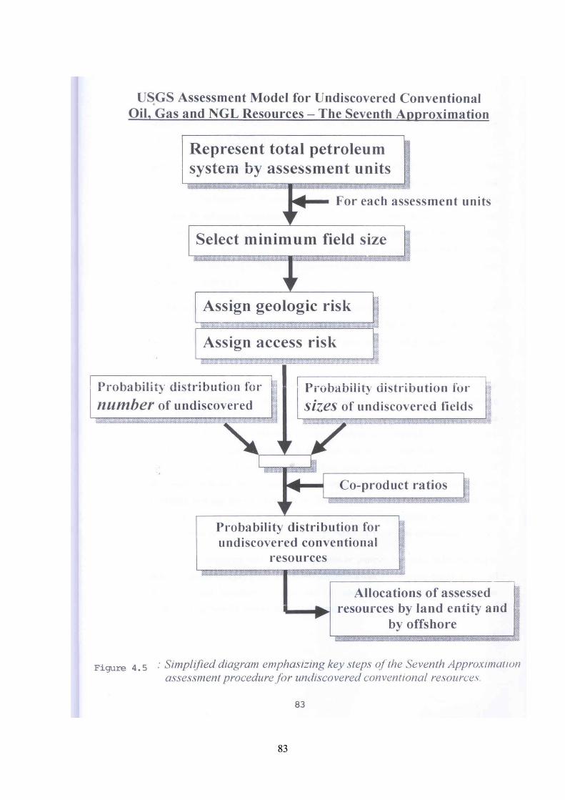
83

resources contained within the AU, such as the amount of gas in gas fields, or oil in oil fields and

their co-products.

Ratios of liquids to gas and ancillary data such as the composition of the gas or oil, drilling

depths, and depths of water are entered onto the form and allocations are made as to the location

of the resource (offshore vs onshore). In this study, these data are used to calculate undiscovered

resources of natural gas liquids and to allocate those resources to the onshore and offshore

portions of Bangladesh . Data used in this study reflect the known field size data provided by

Petrobangla and these fields were not grown in this analysis. Only undiscovered technically

recoverable resources were estimated in this study.

In HCU/NPD Assessment Geological and geo-chemical data together with information about

hydrocarbon discoveries and shows have been used to define petroleum systems, provinces and

plays. All discoveries and prospects have been evaluated and assigned to a specific play.

All prospects, with their key resource parameters were loaded into soft ware GeoX, to serve as

the prospect database. Each individual prospect and lead was evaluated according to geological

knowledge, taking into account the type and quality of the data. For each reservoir parameter a

range of values was selected and the data were loaded into a specific probability distribution. For

most of the parameters used to calculate volumes a triangular distribution was commonly used.

This type of distribution was selected because it gives a better spread in the low and high end than

a normal and log normal distribution. The simulated result for each prospect was recorded and the

prospect stored in GeoX under the appropriate play, petroleum system and area/ block. In this

manner the prospect database was established.

When all the prospects were loaded, they could be grouped and analyzed according to area,

petroleum system, play, and so on. Likewise a size distribution can be displayed and risked and

unranked resources can be calculated. These data are useful for guiding the imputs for estimating

the total undiscovered potential.

84

In the eastern part of the country discoveries prove that all the three defined petroleum system

works, hence they are proved systems. On the contrary, there are no discoveries in the petroleum

systems defined in the western part and they therefore represent unproved systems. There is a risk

associated with not only the prospects, but with the concept that defines the petroleum system.

This risk is broken down from the petroleum system to each play within the system, and is

assigned as a general play risk for all prospects within a specific play. In addition there is an

individual prospect risk. Hence, the risked volumes for these prospects are the result of both the

prospect and the play risk.

4.5 Summary of Undiscovered Resource Assessment

With a view to formulate plans for pragmatic hydrocarbon exploration activities a

number of undiscovered resource assessment have been conducted for Bangladesh over

the years. Some of these studies covered the entire country and the others are limited to

specific areas or known prospects only. Therefore these results are not comparable on an

apple-to-apple basis. However, in order to determine the acceptability and representatives,

the studies conducted during the period 1986 to 2001 are reviewed as under:

4.5.1 Welldrill/ Overseas Development Agencies (ODA) UK, 1986

BOGMC and Welldrill, (ODA) had taken up an exploration program of 8000 km2

area in the Hinge Zone (covering greater Kushtia and part of Jessore), and

identified 21 prospects and 3 leads on the basis of analysis of 2646 km multi-fold

seismic data. The study concluded a total undiscovered unrisked gas resource

potential of 7.55Tcf in the identified prospects.

4.5.2 Hydrocarbon Habitat Study Project (HHSP), 1986

The study conducted with technical support of Welldrill, UK covered both eastern and

western parts of Bangladesh. It identified 44 prospects and Reef Plays (Hinge Zone) with an

estimated maximum unrisked gas-in-place potential of 42.8 Tcf. Out of the estimated total

potential 22 Tcf was identified in 20 anticlinal prospects within Eastern Folded Belt, 16.4

Tcf was allocated for leads and prospects identified within the western shelf,

85

and the remaining quantities were estimated for the more risky buried hills and slope pinch-

out prospects.

4.5.3 German Geological Advisory Group (GGAG),1986

The GGAG study was confined mostly to the eastern part of the country. They identified

only 9 prospects with an unrisked and risked recoverable mean gas resource potential of

6.24 Tcf and 1.76 Tcf respectively. Table-4.1 shows a summary of GGAG estimates.

Table-4.1 Summary of Undiscovered Gas Resource Assessment by GGAG (1986)

TCF

Risking status

Minimum Mean Maximum Remarks

Unrisked

5.04

6.24

7.75

Risked

0.95 1.76 3.33

9 Prospects, Mostly in Eastern part

4.5.4 Anglo-Scandinavian Petroleum Group, 1988

The above Group conducted a hydrocarbon resource potential study of the greater

Mymensingh area and established a gross stratigraphic and structural relationship of the

area based on limited seismic and well data. The study identified 9 leads with an estimated

recoverable (unrisked) gas potential of 7.07 Tcf.

4.5.5 Bangladesh Study Group, 1989

Above Group comprising of Trend International Ltd., Indemitisu Oil Development Co. Ltd.,

Repsol Exploration Indonesia and Eurafrep S.A conducted a joint technical study on

hydrocarbon potential of Bangladesh excluding Block 13,14 and offshore areas. They

identified 130 leads and prospects and estimated an unrisked mode recoverable gas resource

potential of 112 Tcf .

86

4.5.6 Shell Bangladesh Exploration B. V., 1999.

In a paper named 'Gas Resource Estimation - Managing Risk' dated 20th

November Shell reported a total gas resource base of 38 Tcf for Bangladesh. This

included five classifications namely, unidentified potential, cumulative production,

mature reserves, immature reserves and identified potential. But no categorywise

breakdown was provided in the said paper.

4.5.7 Unocal Corporation, 2000.

In March,2000 Unocal reported a total gas resource base of Bangladesh amounting to 41.1

Tcf. This included Field Discoveries of 16.1 Tcf, Field Growth of 11.8 Tcf and New Field

Discoveries (in Block, 7,11,12,13,14 and 20) of 13.2 Tcf.

The above stated Field Growth was said to be the `additional probable` reserve from the

application of advance technologies to the existing gas fields.

The ‘New Field Discoveries’ on the other hand comprised of potential undiscovered gas

resources from the identified prospects and leads in the stated six Blocks.

4.5.8 USGS World Petroleum Assessment 2000

U.S. Geological Survey World Energy Assessment Team made an assessment of

Undiscovered Oil & Gas Resources in the Ganges-Brahmaputra Delta (Geologic

Province 8047) covering Bangladesh, India and Myanmar as a part of their World

Petroleum Assessment 2000. This Geologic Province comprised of Jalangi-

Sylhet/Burdwan Composite Total Petroleum System or the Western Shelf and

Slope Assessment Unit and the Jenam/Bhuban Bokabil Total Petroleum System.

The latter was sub-divided into two assessment units-the Central Basin Assessment

Unit and Eastern Fold Belt Assessment Unit. These three Assessment Units cover

most of the geographical area of Bangladesh and extends about 400 km into the

Bay of Bengal.

87

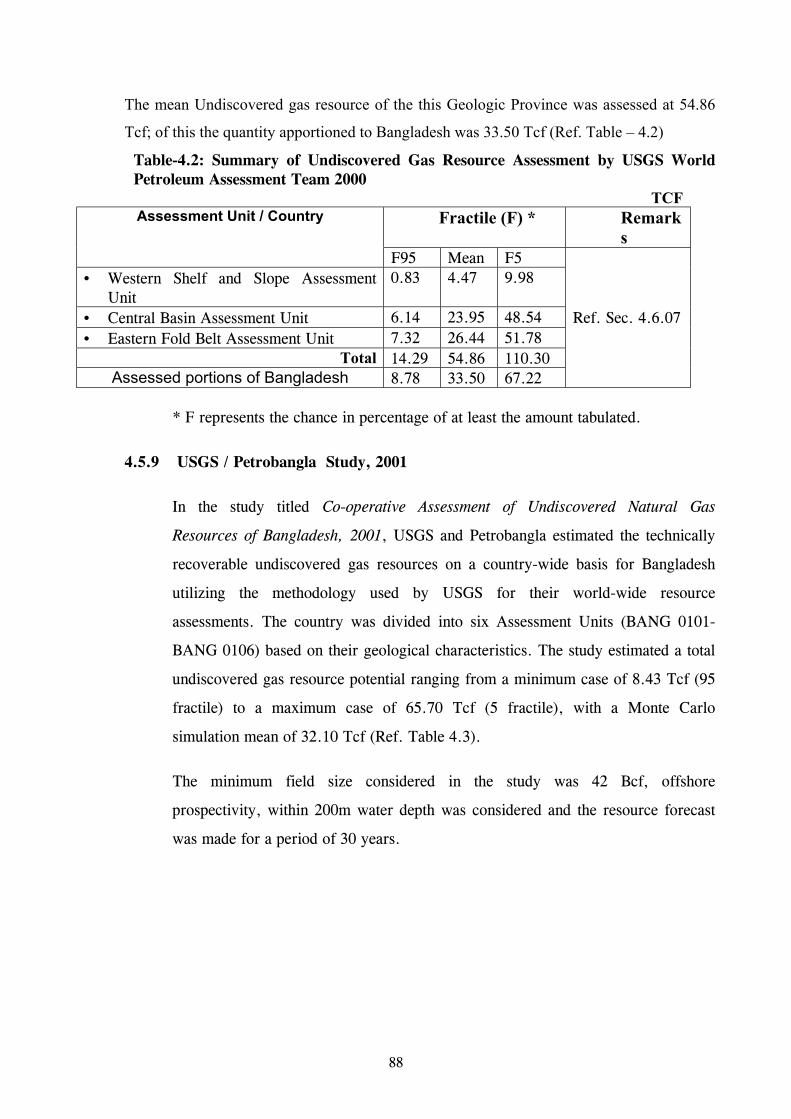
The mean Undiscovered gas resource of the this Geologic Province was assessed at 54.86

Tcf; of this the quantity apportioned to Bangladesh was 33.50 Tcf (Ref. Table – 4.2)

Table-4.2: Summary of Undiscovered Gas Resource Assessment by USGS World Petroleum Assessment Team 2000

TCF Fractile (F) * Remark

s Assessment Unit / Country

F95 Mean F5 • Western Shelf and Slope Assessment

Unit 0.83 4.47 9.98

• Central Basin Assessment Unit 6.14 23.95 48.54 • Eastern Fold Belt Assessment Unit 7.32 26.44 51.78

Total 14.29 54.86 110.30 Assessed portions of Bangladesh 8.78 33.50 67.22

Ref. Sec. 4.6.07

* F represents the chance in percentage of at least the amount tabulated.

4.5.9 USGS / Petrobangla Study, 2001

In the study titled Co-operative Assessment of Undiscovered Natural Gas

Resources of Bangladesh, 2001, USGS and Petrobangla estimated the technically

recoverable undiscovered gas resources on a country-wide basis for Bangladesh

utilizing the methodology used by USGS for their world-wide resource

assessments. The country was divided into six Assessment Units (BANG 0101-

BANG 0106) based on their geological characteristics. The study estimated a total

undiscovered gas resource potential ranging from a minimum case of 8.43 Tcf (95

fractile) to a maximum case of 65.70 Tcf (5 fractile), with a Monte Carlo

simulation mean of 32.10 Tcf (Ref. Table 4.3).

The minimum field size considered in the study was 42 Bcf, offshore

prospectivity, within 200m water depth was considered and the resource forecast

was made for a period of 30 years.

88

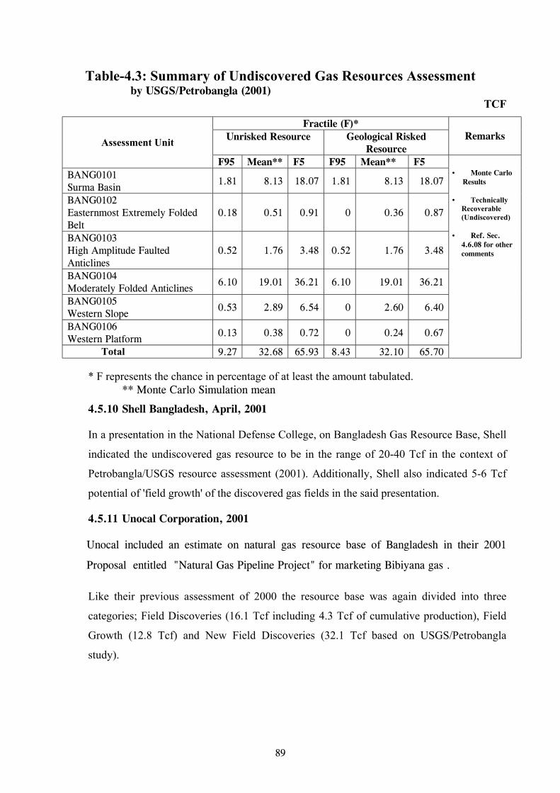
Table-4.3: Summary of Undiscovered Gas Resources Assessment by USGS/Petrobangla (2001)

TCF

Fractile (F)* Unrisked Resource Geological Risked

Resource Remarks Assessment Unit

F95 Mean** F5 F95 Mean** F5 BANG0101 Surma Basin

1.81 8.13 18.07 1.81 8.13 18.07

BANG0102 Easternmost Extremely Folded Belt

0.18 0.51 0.91 0 0.36 0.87

BANG0103 High Amplitude Faulted Anticlines

0.52 1.76 3.48 0.52 1.76 3.48

BANG0104 Moderately Folded Anticlines

6.10 19.01 36.21 6.10 19.01 36.21

BANG0105 Western Slope

0.53 2.89 6.54 0 2.60 6.40

BANG0106 Western Platform

0.13 0.38 0.72 0 0.24 0.67

Total 9.27 32.68 65.93 8.43 32.10 65.70

• Monte Carlo Results • Technically

Recoverable (Undiscovered)

• Ref. Sec.

4.6.08 for other comments

* F represents the chance in percentage of at least the amount tabulated. ** Monte Carlo Simulation mean

4.5.10 Shell Bangladesh, April, 2001

In a presentation in the National Defense College, on Bangladesh Gas Resource Base, Shell

indicated the undiscovered gas resource to be in the range of 20-40 Tcf in the context of

Petrobangla/USGS resource assessment (2001). Additionally, Shell also indicated 5-6 Tcf

potential of 'field growth' of the discovered gas fields in the said presentation.

4.5.11 Unocal Corporation, 2001

Unocal included an estimate on natural gas resource base of Bangladesh in their 2001

Proposal entitled "Natural Gas Pipeline Project" for marketing Bibiyana gas .

Like their previous assessment of 2000 the resource base was again divided into three

categories; Field Discoveries (16.1 Tcf including 4.3 Tcf of cumulative production), Field

Growth (12.8 Tcf) and New Field Discoveries (32.1 Tcf based on USGS/Petrobangla

study).

89

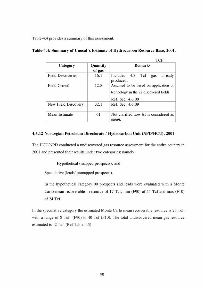
Table-4.4 provides a summary of this assessment.

Table-4.4: Summary of Unocal`s Estimate of Hydrocarbon Resource Base, 2001. TCF

Category

Quantity of gas

Remarks

Field Discoveries 16.1 Includes 4.3 Tcf gas already produced.

Field Growth 12.8 Assumed to be based on application of

technology in the 22 discovered fields.

Ref. Sec. 4.6.09 New Field Discovery 32.1

Ref. Sec. 4.6.09

Mean Estimate 61

Not clarified how 61 is considered as mean.

4.5.12 Norwegian Petroleum Directorate / Hydrocarbon Unit (NPD/HCU), 2001

The HCU/NPD conducted a undiscovered gas resource assessment for the entire country in

2001 and presented their results under two categories; namely:

Hypothetical (mapped prospects), and

Speculative (leads/ unmapped prospects).

In the hypothetical category 90 prospects and leads were evaluated with a Monte

Carlo mean recoverable resource of 17 Tcf, min (F90) of 11 Tcf and max (F10)

of 24 Tcf.

In the speculative category the estimated Monte Carlo mean recoverable resource is 25 Tcf,

with a range of 8 Tcf (F90) to 40 Tcf (F10). The total undiscovered mean gas resource

estimated is 42 Tcf. (Ref Table-4.5)

90

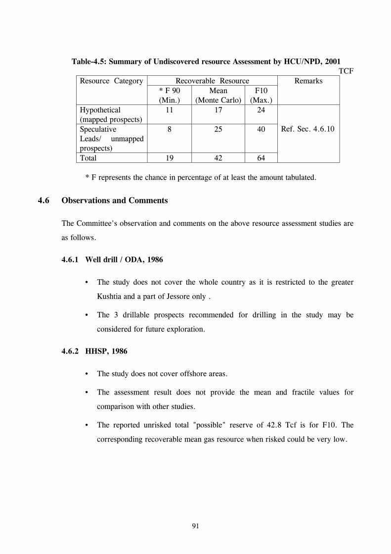
Table-4.5: Summary of Undiscovered resource Assessment by HCU/NPD, 2001

TCF Recoverable Resource Resource Category

* F 90 (Min.)

Mean (Monte Carlo)

F10 (Max.)

Remarks

Hypothetical (mapped prospects)

11 17 24

Speculative Leads/ unmapped prospects)

8 25 40

Total 19 42 64

Ref. Sec. 4.6.10

* F represents the chance in percentage of at least the amount tabulated.

4.6 Observations and Comments

The Committee's observation and comments on the above resource assessment studies are

as follows.

4.6.1 Well drill / ODA, 1986

• The study does not cover the whole country as it is restricted to the greater

Kushtia and a part of Jessore only .

• The 3 drillable prospects recommended for drilling in the study may be

considered for future exploration.

4.6.2 HHSP, 1986

• The study does not cover offshore areas.

• The assessment result does not provide the mean and fractile values for

comparison with other studies.

• The reported unrisked total "possible" reserve of 42.8 Tcf is for F10. The

corresponding recoverable mean gas resource when risked could be very low.

91

4.6.3 GGAG, 1986

• This study also does not cover the whole country as it is limited to the eastern

part.

• For the study area out of 9 prospects 6 were drilled of which 5 were gas

discoveries –– actual reserves are also quite close to the prognosed reserves

(1.70 Tcf vs 1.54 Tcf). The study quality, therefore, is considered to be very

high.

4.6.4 Anglo-Scandinavian, 1988

• The study is restricted to a very limited area, and that too is based on a very

limited database.

4.6.5 Bangladesh Study Group, 1989

• The study claims to be based on good database and to cover almost the entire

country giving a unrisked mode recoverable potential of 112 Tcf. This appears

to be very optimistic, since the subsequent studies with more reliable data and

applications of up-to-date technologies by various study groups have never

come up with such high numbers.

• Further, Blockwise results are provided as estimated Min, Mode and Max

Recoverable Reserve in MMBOE which may be considered optimistic based on

the "2nd Round Bidding" response for various PSC Blocks. For instance, for

Block 4 the Estimated Recoverable Reserve stated to be 2000 MMBOE in the

identified leads, with an Upside Potential of 1750 MMBOE. But no genuine

interest was received for such a supposedly prolific acreage.

4.6.6 Shell Bangladesh E&D, 1999 and 2001

• The 1999 Resource base assessment of Shell did not provide their estimated

number for undiscovered gas resource. On the other hand the 2001 report

indicated a range of 20 - 40 Tcf with reference to USGS/PB studies without

92

giving any analysis. The results, therefore, appear to be only indicative in nature.

4.6.7 USGS World Petroleum Assessment 2000

• The assessment was not based on a country boundary of Bangladesh. The result of

the Geologic Province of Ganges Brahmaputra Delta was apportioned to this

country.

• The study lacked adequate input data for geological description for hydrocarbon

potentials, which was subsequently improved in the USGS/Petrobangla Joint Study.

• The minimum field size considered for assessment was 2 MMBOE grown (> 1

MMBOE). The growth function assumed are taken from the U.S. experience of

their lower- 48 states. This analogy may not be applicable for Bangladesh. The

minimum field size also must be considered very optimistic.

4.6.8 USGS/Petrobangla Undiscovered Gas Resource Assessment, 2001.

• The summary Table of the Report indicates risked resource range of 8.43 Tcf (F95)

to 65.70 Tcf (F5) with a mean of 32.10 Tcf. The unrisked assessment numbers are

also shown in the Table 4.3.

• The USGS methodology applied in the study is endorsed by American Association

of Petroleum Geologist (AAPG).

• 30 year's period as the basis for resource forecast as well as the minimum field size

(42 Bcf) considered in the study seems to be quite reasonable for a developing

country like Bangladesh in the light of anticipated exploration and infrastructural

developments.

• The Study results provide technically recoverable resource, meaning recovery

factors are already built-in in the estimates. But commerciality of the resource

assessment are not considered.

93

4.6.9 Unocal Corp. 2000 and 2001

• The total resource base estimated by Unocal covers Field Discoveries (incl.

produced gas), Field Growth and New field Discoveries i.e. undiscovered

resources. Such an aggregation of quantities of widely varying certainties is

misleading.

• Regarding 'Field Growth' it should be noted that this concept is only valid for

producing fields; but Unocal has applied their assumed growth factors for all the

gas fields irrespective of their production status.

• Considering 'Field Growth' as 'additional probable' reserve as shown by Unocal in

their 2001 Report is not consistent with SPE/WPC definitions.

• Use of the terminology "New Fields Discoveries" for the undiscovered gas

resources / prospects /leads is misleading.

• In the 2001 assessment Unocal has placed PB/USGS countrywide assessment

number in the name of ‘New Field Discoveries’ under possible reserve categories.

This also contradicts SPE/WPC definitions and is therefore misleading

4.6.10 NPD/HCU, 2001

• The Undiscovered resource assessment by NPD/HCU has been done by using

GeoX software and available latest database . The study results have also rightly

identified the resources into hypothetical and speculative categories for the mapped

and unmapped prospects/leads.

• The minimum prospect size was chosen as 10 Bcf for onshore and 50 Bcf offshore.

This appears optimistic since a much larger offshore gas discovery ( Kutubdia, 468

Bcf ) is yet to be commercial even 25 years after its discovery. Likewise, the 98

Bcf onshore discovery Semutang (discovered in1969) is also awaiting development

by the PSC `Operator' for many years.

• The Petroleum System-wise and the summarised in-place resource and

recoverable resource analysis indicate a field recovery efficiency of over 72%.

94

This appear to be an optimistic assumption of undiscovered resource before knowing

any physical and dynamic conditions of the potential hydrocarbon accumulations.

• The study appears to be an open-ended forecast, as no specific forecast period has

been considered . This may not be helpful for taking up realistic exploration

strategies and corresponding infrastructural developments.

• Of the total 42 Tcf of mean recoverable resource, 25 Tcf is 'Speculative' based on

geological evaluation of different Petroleum Systems using Monte Carlo Simulation.

This also may be considered optimistic in view of recent negative outcome of several

offshore drillings including an over-pressure prospect at South Sangu.

4.7 Conclusions

1. The quality of a resource assessment study can best be evaluated by the `Performance

Indicator’ that would reflect the volume of undiscovered resource which is actually converted

to reserve through exploration activities. Going by this Indicator, the 1986 GGAG study should

be considered a very high quality work as the actual discovered reserve closely matched with the

pre-drilling resource assessment. But, the GGAG study was confined to the eastern part of the

country only. And, with respect to the series of assessment studies, conducted during 1999-2001

for the whole country, it is too early to quantify their performance since very few exploration

drilling have been done based on their recommendations so far.

2. The undiscovered resource assessment is basically a combination of hypothetical and

speculative numbers with little or no economic considerations. Therefore, these numbers may

only be used for petroleum exploration purposes and not for petroleum exploitation planning.

3. Of all the resources studies, USGS-Petrobangla and HCU-NPD studies are more recent,

extensive and systematically conducted. But considering the comments in the previous section,

95

it is concluded that the 2001 USGS-Petrobangla gas resource assessment may be considered to reflect

the country’s undiscovered gas resources. According to this study, the undiscovered Gas Resources of

the country ranges from 8.43 Tcf (95% chance) to 65.70 Tcf (05% chance) with a simulation mean of

32.10 Tcf.

4.8 References

Alam. K., Hasan. A. K. M. S Kahn. M. R., And Whitney. J. W. 1990. Geological map of Bangladesh : Geological Survey of Bangladesh Geological Map. Scale 1: 1,000,000. Bangladesh Oil Gas and Mineral Corporation: “Habitat of Hydrocarbons in Bangladesh -1986 “. Report on the Hydrocarbon Habitat Study (1984-86). Bangladesh Oil Gas and Mineral Corporation: “ The Oil and Gas Seismic Exploration Project, The Hinge Zone Survey, Western Bangladesh, BOGMC/WELDRILL -1986. Bangladesh study group: “Hydrocarbon Potential of Bangladesh” (Studied by Trend international Ltd., Idemitsu Oil Development Co., Ltd. & Repsol exploration Indonesia Eurafrep S. A) September 15, 1989 to January 15, 1990. German Geological Advisory Group with Petrobangla. “Hydrocarbon Reserves in Bangladesh”. M. Eder & G. Hildebrand. May 1986. Schmoker, J. W., and Klett, T. R., 1999, U.S. Geological Survey assessment model for undiscovered conventional oil, gas and NGL resources- The Servant Approximation: U.S. Geological Survey Bulletin 2165 Version 1.0. Shamsuddin, A. K. M. and Abdullah, S. K. M., 1997, Geologic evolution of the Bengal Basin and its implication in hydrocarbon exploration in Bangladesh: Indian Journal of Geology, vol.69, no.2, p.93-121 Hydrocarbon Unit (HCU) of the Energy and Mineral Resource Division and ;the Norwegian Petroleum Directorate, “ Bangladesh Petroleum Potential and Resource Assessment 2001,” January 2002. Petrobangla and USGS Joint Resource Assessment Team, “U.S. Geological Survey –Petrobangla Cooperative Assessment of Undiscovered Natural Gas Resources of Bangladesh,” January 2001. Shell Bangladesh Exploration and Development, “ Bangladesh Power and Energy Today, “National Defence College, Dhaka, Bangladesh, April 2001.

96

Shell Bangladesh Exploration and Development, “ Gas Resource Estimation-Managing Risk,” Bangladesh Institute of Law and International Affairs, Dhaka, November 1999. Unocal Corporation: “Bangladesh Natural Gas Pipeline Project” April 2001. Unocal Corporation: “Bangladesh Resource Assessment” March 2000. World Energy Assessment Team. 2000. U. S Geological Survey World Petroleum Assessment 2000-Description and results: USGS Digital Data Series DDS-60 Multi Disc Set, Version 1.0.

97

98

99

100

101

REPORT OF THE COMMITTEE - sdnbd.org · REPORT OF THE COMMITTEE ... fractile) to 65.70 Tcf ......

Documents

Transcript of REPORT OF THE COMMITTEE - sdnbd.org · REPORT OF THE COMMITTEE ... fractile) to 65.70 Tcf ......