Report Network Modelling

Network modelling: Theory and Simulation

Zoppi Samuele 202769

Ferro Demetrio 207872

Minetto Alex 211419

Network modelling: Theory and Simulation Laboratory 1

Laboratory 1

Task 1: The M/M/1 queue

Consider an M/M/1 queue.Plot the performance of the queue versus load in terms of:

· Average queuing delay

· Probability that the server is idle (i.e., fraction of time that the server is idle)

Verify Little’s law. Compare simulation and analytical results.

M/M/1 Queue

λ µ

Figure 1: Model of an M/M/1 Queue

The queueing system is modeled as follows:

· Arrivals are Poisson distributed with rate λ.

· Service times are Exponentially distributed with pa-rameter µ.

The stochastic behaviour can be modeled as a Continu-ous Time Markov Chain, whose state space refers to thenumber of customers in the system.

The chain has an infinite number of states, but it has a stationary distribution, hence preservesergodicity, just for λ < µ. The main indices of the system are the following:

· E[L], Average number of customers in the system: from the stationary distribution, it can beeasily computed.

· E[Ts], Average serving time: since service times are Exp(µ), it is always equal to 1µ .

· E[T ], Average time spent in the queue: it can be computed with Little’s Result: E[T ] = E[L]λ

· E[Tw], Average waiting time: it can be computed by difference: E[Tw] = E[T ] − E[Ts].

Once we considered all the theoretical issues, we proceeded with simulations, by computing:

Average queueing delay

In order to get to a global overview of the results when the load factor ρ, vary in ]0, 1[, we wrote abash script which executes the provided C program for the simulation for different values of ρ.

We fixed µ = 1 and let λ, hence ρ, vary in ]0, 1[.

A complete simulation consisted in letting λ vary from 0.001 to 0.999 with step 0.001 whose outputwill report here in plots.

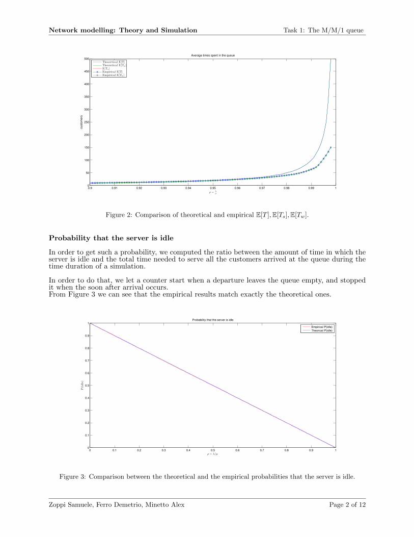
In Figure 2 is reported an overall view of the comparison between theoretical and empirical Timesspent in the queue.

The average time spent Serving is supposed to be constant and equal to E[Ts] = 1µ = 1, whereas the

time spent waiting E[Tw] and the total time E[T ] are obtained from the simulation and comparedto the theoretical ones.

As we can see, the theoretical results are very likely until the condition ρ < 1 is satisfied.

Zoppi Samuele, Ferro Demetrio, Minetto Alex Page 1 of 12

Network modelling: Theory and Simulation Task 1: The M/M/1 queue

0.9 0.91 0.92 0.93 0.94 0.95 0.96 0.97 0.98 0.99 10

50

100

150

200

250

300

350

400

450

500Average times spent in the queue

ρ = λµ

custo

mers

Theoretical E[T]Theoretical E[Tw]E[Ts]Empirical E[T]Empirical E[Tw]

Figure 2: Comparison of theoretical and empirical E[T ],E[Ts],E[Tw].

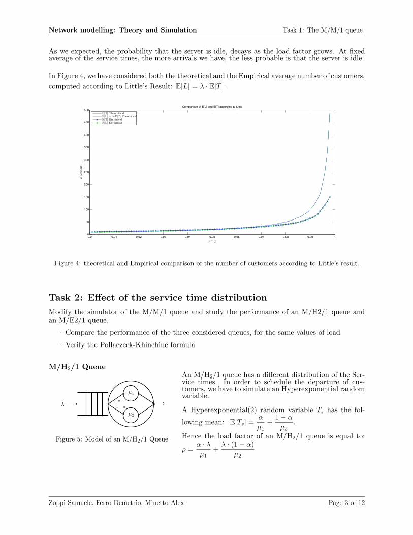
Probability that the server is idle

In order to get such a probability, we computed the ratio between the amount of time in which theserver is idle and the total time needed to serve all the customers arrived at the queue during thetime duration of a simulation.

In order to do that, we let a counter start when a departure leaves the queue empty, and stoppedit when the soon after arrival occurs.From Figure 3 we can see that the empirical results match exactly the theoretical ones.

0 0.1 0.2 0.3 0.4 0.5 0.6 0.7 0.8 0.9 10

0.1

0.2

0.3

0.4

0.5

0.6

0.7

0.8

0.9

1

ρ = λ/µ

P(idle)

Probability that the server is idle

Empirical P(idle)

Theorical P(idle)

Figure 3: Comparison between the theoretical and the empirical probabilities that the server is idle.


Network modelling: Theory and Simulation Task 1: The M/M/1 queue

As we expected, the probability that the server is idle, decays as the load factor grows. At fixedaverage of the service times, the more arrivals we have, the less probable is that the server is idle.

In Figure 4, we have considered both the theoretical and the Empirical average number of customers,

computed according to Little’s Result: E[L] = λ · E[T ].

0.9 0.91 0.92 0.93 0.94 0.95 0.96 0.97 0.98 0.99 10

50

100

150

200

250

300

350

400

450

500Comparison of E[L] and E[T] according to Little

ρ = λµ

cu

sto

me

rs

E[T] TheoreticalE[L] = λ·E[T] TheoreticalE[T] EmpiricalE[L] Empirical

Figure 4: theoretical and Empirical comparison of the number of customers according to Little’s result.

Task 2: Effect of the service time distribution

Modify the simulator of the M/M/1 queue and study the performance of an M/H2/1 queue andan M/E2/1 queue.

· Compare the performance of the three considered queues, for the same values of load

· Verify the Pollaczeck-Khinchine formula

M/H2/1 Queue

λα

1 − α

µ1

µ2

Figure 5: Model of an M/H2/1 Queue

An M/H2/1 queue has a different distribution of the Ser-vice times. In order to schedule the departure of cus-tomers, we have to simulate an Hyperexponential randomvariable.

A Hyperexponential(2) random variable Ts has the fol-

lowing mean: E[Ts] =α

µ1+

1 − α

µ2.

Hence the load factor of an M/H2/1 queue is equal to:

ρ =α · λµ1

+λ · (1 − α)

µ2


Network modelling: Theory and Simulation Task 2: Effect of the service time distribution

M/E2/1 Queue

λ µ1 µ2

Figure 6: Model of an M/E2/1 Queue

This time the Service times have a different dis-tribution. By supposing that the service is com-posed of two phases, it’s easy to see that theamount of time spent in service is the sum of thetime spent in the two phases. In order to sched-ule the departure of customers, we have to simu-late Erlang distribution made of two contributions(E2).

An Erlang(2) random variable Ts has the following mean:

E[Ts] =1

µ1+

1

µ2, and load factor: ρ =

λ

µ1+

λ

µ2=λ

µ.

In order to evaluate the performances of the 3 queues, we compared the results for:

· M/M/1 Queue with Exponential service times, with parameter µ = 1.

· M/H2/1 Queue with Hyperexponential(2) service times, with µ1 = 1, µ2 = 1, α = 12 .

· M/E2/1 Queue with Erlang(2) service times: with µ1 = 2, µ2 = 2.

By letting hence ρ, vary in ]0, 1[, we wanted to evaluate the performances of the three queueingsystems, for the same values of load.

0.97 0.975 0.98 0.985 0.99 0.9950

50

100

150

200

250

300

350

400

450

500

ρ

tim

e

Average Time spent in the queue

MM1 E[T

s] Theoretical

MM1 E[Tw

] Theoretical

MM1 E[T] TheoreticalMH

21 E[T

s] Theoretical

MH21 E[T

w] Theoretical

MH21 E[T] Theoretical

ME21 E[T

s] Theoretical

ME21 E[T

w] Theoretical

ME21 E[T] Theoretical

MM1 E[Tw

] Empirical

MM1 E[T] EmpiricalMH

21 E[T

w] Empirical

MH21 E[T] Empirical

ME21 E[T

w] Empirical

ME21 E[T] Empirical

Figure 7: Comparison of theoretical and empirical E[Ts],E[Tw],E[T ] in the three queueing systems.

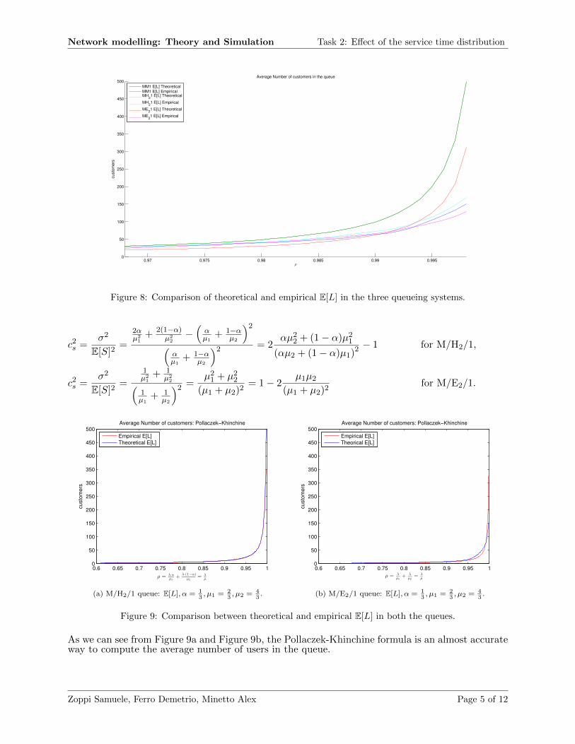
In Figure 7 and Figure 8 we reported the behaviour of the three queues, both empirical and theo-retical data.

From the comparison of the results, we could see that in terms of average number of users andaverage time spent in the queue, the M/E2/1 has better performances than the M/M/1, which stillhas better performances than the M/H2/1.

From the Pollanczeck-Khinchine, we shall consider:

E[L] = ρ+ρ2(1 + c2

s)

2(1 − ρ), E[T ] =

E[L]

λ= µ+

ρ(1 + c2s)

2µ(1 − ρ)where cs =

σsE[S]


Network modelling: Theory and Simulation Task 2: Effect of the service time distribution

0.97 0.975 0.98 0.985 0.99 0.9950

50

100

150

200

250

300

350

400

450

500

ρ

custo

me

rs

Average Number of customers in the queue

MM1 E[L] Theoretical

MM1 E[L] EmpiricalMH

21 E[L] Theoretical

MH21 E[L] Empirical

ME21 E[L] Theoretical

ME21 E[L] Empirical

Figure 8: Comparison of theoretical and empirical E[L] in the three queueing systems.

c2s =

σ2

E[S]2=

2αµ2

1+ 2(1−α)

µ22

−(αµ1

+ 1−αµ2

)2

(αµ1

+ 1−αµ2

)2 = 2αµ2

2 + (1 − α)µ21

(αµ2 + (1 − α)µ1)2 − 1 for M/H2/1,

c2s =

σ2

E[S]2=

1µ2

1+ 1

µ22(

1µ1

+ 1µ2

)2 =µ2

1 + µ22

(µ1 + µ2)2= 1 − 2

µ1µ2

(µ1 + µ2)2for M/E2/1.

0.6 0.65 0.7 0.75 0.8 0.85 0.9 0.95 10

50

100

150

200

250

300

350

400

450

500Average Number of customers: Pollaczek−Khinchine

ρ = λ·αµ1

+ λ·(1−α)µ2

= λµ

cu

sto

me

rs

Empirical E[L]

Theoretical E[L]

(a) M/H2/1 queue: E[L], α = 13, µ1 = 2

3, µ2 = 4

3.

0.6 0.65 0.7 0.75 0.8 0.85 0.9 0.95 10

50

100

150

200

250

300

350

400

450

500Average Number of customers: Pollaczek−Khinchine

ρ =λµ1

+λµ2

=λµ

cu

sto

me

rs

Empirical E[L]

Theorical E[L]

(b) M/E2/1 queue: E[L], α = 13, µ1 = 2

3, µ2 = 4

3.

Figure 9: Comparison between theoretical and empirical E[L] in both the queues.

As we can see from Figure 9a and Figure 9b, the Pollaczek-Khinchine formula is an almost accurateway to compute the average number of users in the queue.


Network modelling: Theory and Simulation Task 3: The M/G/k queue

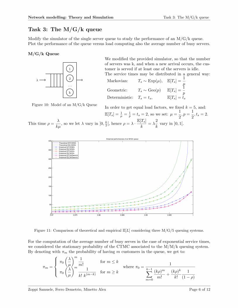
Task 3: The M/G/k queue

Modify the simulator of the single server queue to study the performance of an M/G/k queue.Plot the performance of the queue versus load computing also the average number of busy servers.

M/G/k Queue

1

2

· · ·

k

λ

Figure 10: Model of an M/G/k Queue

We modified the provided simulator, so that the numberof servers was k, and when a new arrival occurs, the cus-tomer is served if at least one of the servers is idle.The service times may be distributed in a general way:

Markovian: Ts ∼ Exp(µ), E[Ts] =1

µ

Geometric: Ts ∼ Geo(p) E[Ts] =1

pDeterministic: Ts = ts, E[Ts] = ts

In order to get equal load factors, we fixed k = 5, and:

E[Ts] = 1µ = 1

p = ts = 2, so we set: µ =1

2, p =

1

2, ts = 2.

This time ρ =λ

kµ, so we let λ vary in ]0, k2 [, hence ρ = λ · E[Ts]

k= λ

2

kvary in ]0, 1[.

0.97 0.975 0.98 0.985 0.99 0.995 10

50

100

150

200

250

300

350

400Empirical performances of an M/G/k queue

Theoretical E[T] M/M/k

Theoretical E[L] M/M/k

Empirical E[T] M/M/k

Empirical E[L] M/M/k

Empirical E[T] M/D/k

Empirical E[L] M/D/k

Empirical E[T] M/Geom/k

Empirical E[L] M/Geom/k

Figure 11: Comparison of theoretical and empirical E[L] considering three M/G/5 queuing systems.

For the computation of the average number of busy serves in the case of exponential service times,we considered the stationary probability of the CTMC associated to the M/M/k queuing system.By denoting with πm the probability of having m customers in the queue, we get to:

πm =

π0

(λ

µ

)m 1

m!for m ≤ k

π0

(λ

µ

)m 1

k! k(m−k)for m ≥ k

where π0 =1

k−1∑m=0

(kρ)m

m!+

(kρ)k

k!

1

(1 − ρ)


Network modelling: Theory and Simulation Task 3: The M/G/k queue

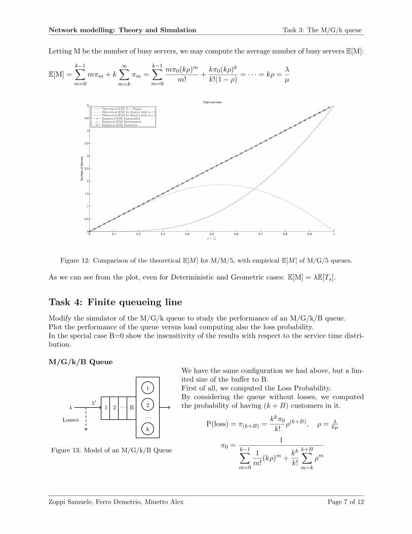
Letting M be the number of busy servers, we may compute the average number of busy servers E[M]:

E[M] =

k−1∑m=0

mπm + k

∞∑m=k

πm =

k−1∑m=0

mπ0(kρ)m

m!+kπ0(kρ)k

k!(1 − ρ)= · · · = kρ =

λ

µ

0 0.1 0.2 0.3 0.4 0.5 0.6 0.7 0.8 0.9 10

0.5

1

1.5

2

2.5

3

3.5

4

4.5

5

ρ = λmµ

Num

ber

of

Serv

ers

Total overview

Theoretical E[M] Ts ∼ Exp(µ)Theoretical E[M] for Exp(µ) with m < k

Theoretical E[M] for Exp(µ) with m ≥ k

Empirical E[M] ExponentialEmpirical E[M] DeterministicEmpirical E[M] Geometric

Figure 12: Comparison of the theoretical E[M ] for M/M/5, with empirical E[M ] of M/G/5 queues.

As we can see from the plot, even for Deterministic and Geometric cases: E[M] = λE[Ts].

Task 4: Finite queueing line

Modify the simulator of the M/G/k queue to study the performance of an M/G/k/B queue.Plot the performance of the queue versus load computing also the loss probability.In the special case B=0 show the insensitivity of the results with respect to the service time distri-bution.

M/G/k/B Queue

1 2 · · · B

1

2

· · ·

k

λ

Losses

λ′

Figure 13: Model of an M/G/k/B Queue

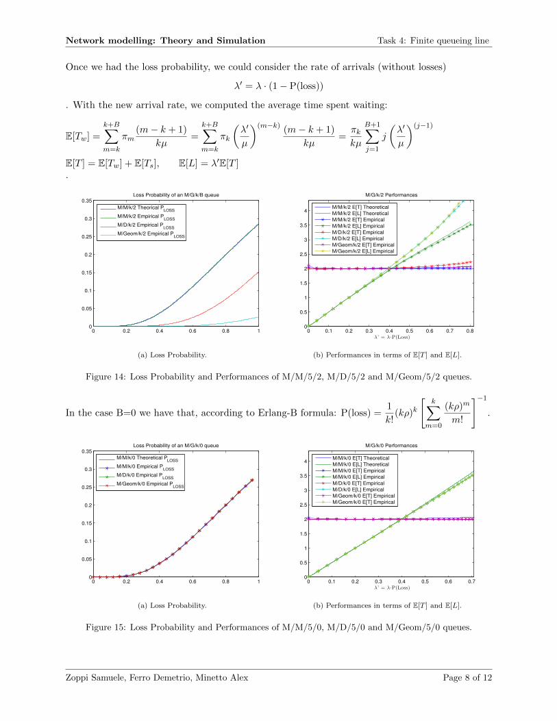
We have the same configuration we had above, but a lim-ited size of the buffer to B.First of all, we computed the Loss Probability.By considering the queue without losses, we computedthe probability of having (k +B) customers in it.

P(loss) = π(k+B) =kkπ0

k!ρ(k+B), ρ = λ

kµ

π0 =1

k−1∑m=0

1

m!(kρ)m +

kk

k!

k+B∑m=k

ρm


Network modelling: Theory and Simulation Task 4: Finite queueing line

Once we had the loss probability, we could consider the rate of arrivals (without losses)

λ′ = λ · (1 − P(loss))

. With the new arrival rate, we computed the average time spent waiting:

E[Tw] =

k+B∑m=k

πm(m− k + 1)

kµ=

k+B∑m=k

πk

(λ′

µ

)(m−k) (m− k + 1)

kµ=πkkµ

B+1∑j=1

j

(λ′

µ

)(j−1)

E[T ] = E[Tw] + E[Ts], E[L] = λ′E[T ].

0 0.2 0.4 0.6 0.8 10

0.05

0.1

0.15

0.2

0.25

0.3

0.35Loss Probability of an M/G/k/B queue

M/M/k/2 Theorical PLOSS

M/M/k/2 Empirical PLOSS

M/D/k/2 Empirical PLOSS

M/Geom/k/2 Empirical PLOSS

(a) Loss Probability.

0 0.1 0.2 0.3 0.4 0.5 0.6 0.7 0.80

0.5

1

1.5

2

2.5

3

3.5

4

λ’ = λ·P(Loss)

M/G/k/2 Performances

M/M/k/2 E[T] Theoretical

M/M/k/2 E[L] Theoretical

M/M/k/2 E[T] Empirical

M/M/k/2 E[L] Empirical

M/D/k/2 E[T] Empirical

M/D/k/2 E[L] Empirical

M/Geom/k/2 E[T] Empirical

M/Geom/k/2 E[L] Empirical

(b) Performances in terms of E[T ] and E[L].

Figure 14: Loss Probability and Performances of M/M/5/2, M/D/5/2 and M/Geom/5/2 queues.

In the case B=0 we have that, according to Erlang-B formula: P(loss) =1

k!(kρ)k

[k∑

m=0

(kρ)m

m!

]−1

.

0 0.2 0.4 0.6 0.8 10

0.05

0.1

0.15

0.2

0.25

0.3

0.35Loss Probability of an M/G/k/0 queue

M/M/k/0 Theoretical PLOSS

M/M/k/0 Empirical PLOSS

M/D/k/0 Empirical PLOSS

M/Geom/k/0 Empirical PLOSS

(a) Loss Probability.

0 0.1 0.2 0.3 0.4 0.5 0.6 0.70

0.5

1

1.5

2

2.5

3

3.5

4

λ’ = λ·P(Loss)

M/G/k/0 Performances

M/M/k/0 E[T] Theoretical

M/M/k/0 E[L] Theoretical

M/M/k/0 E[T] Empirical

M/M/k/0 E[L] Empirical

M/D/k/0 E[T] Empirical

M/D/k/0 E[L] Empirical



(b) Performances in terms of E[T ] and E[L].

Figure 15: Loss Probability and Performances of M/M/5/0, M/D/5/0 and M/Geom/5/0 queues.


Network modelling: Theory and Simulation Laboratory 2

Laboratory 2

Task 1: Two M/M/1 queues

Consider two M/M/1 queues in sequence. Implement the simulator to derive the steady state be-havior of the system. Verify the product form solution.

In order to implement the queueing network we modified the simulator, scheduling an arrival inthe second queue at every departure from the first queue. The record of one costumer comingfrom exogenous arrivals is created when it arrives in the first queue, it’s moved from one queue toanother and it’s freed only when it leaves the second queue, leaving the network.We measured the time in which the network was in a specific (k1, k2) condition and we dividedby the total time to get the steady state probabilities πk1,k2 . Finally we compared these empiricalresults with the theoretical product form solution for a network of two M/M/1 queues:

πN = πk1,k2 = π(1)k1

· π(2)k2

= (1 − ρ1)ρk11 · (1 − ρ2)ρk22

In order to verify the product form solution we used µ1 = 1 µ2 = 1 and let λ vary in ]0, 1[ so thatthe two M/M/1 had the same ρ = ρ1 = ρ2, varying in ]0, 1[.

The product form solution reduces to:

πN = πk1,k2 = (1 − ρ)2ρk1+k2

The computation of the probability density functions was implemented in the simulator, and in thefollowing figures (Figure 16, Figure 17) the empirical results are compared to the theoretical ones.

0 0.1 0.2 0.3 0.4 0.5 0.6 0.7 0.8 0.9 10

0.1

0.2

0.3

0.4

0.5

0.6

0.7

0.8

0.9

1

Empirical Pi0,0

Theoretical Pi0,0

Empirical Pi1,1

Theoretical Pi1,1

Empirical Pi2,2

Theoretical Pi2,2

Empirical Pi1,2

Theoretical Pi1,2

Figure 16: Steady state probabilities for π0,0, π1,1, π2,2.


Network modelling: Theory and Simulation Task 2: Effect of the service time distribution and . . .

0 0.2 0.4 0.6 0.8 10

0.01

0.02

0.03

0.04

0.05

0.06

0.07

Empirical Pi1,1

Theoretical Pi1,1

Empirical Pi2,2

Theoretical Pi2,2

Empirical Pi1,2

Theoretical Pi1,2

(a) Steady state probabilities for π1,1, π2,2, π1,2.

0 0.1 0.2 0.3 0.4 0.5 0.6 0.7 0.8 0.9 10

0.5

1

1.5

2

2.5

3

3.5

4

4.5x 10

−3

Empirical Pi10,10

Theorical Pi10,10

Empirical Pi10,5

Theorical Pi10,5

Empirical Pi10,1

Theorical Pi10,1

(b) Steady state probabilities for π0,0, π1,1, π2,2.

Figure 17: Steady state probabilities πk1,k2 : theoretical and empirical.

Task 2: Effect of the service time distribution and first moment

· Consider the case of two queues with different service rate. Evaluate and compare the averagebuffer occupancy of the two queues when µ1 > µ2 and when µ1 ≤ µ2.

· Consider the case of deterministic service times with µ1 ≤ µ2, evaluate and compare the averagebuffer occupancy and the buffer occupancy distribution for the two queues.

We computed the average buffer occupancies adding counters in the code able to track the behaviorof the buffer occupancies over time.We compared the results of the simulator with the following theoretical formula for the bufferoccupancy of an M/M/1 queue:

E[buffer occupancy] = E[Lw] =ρ2

(1 − ρ)

In Figure 18 are reported the plots of the comparison between the ideal M/M/1 and the actualqueueing network.

0.97 0.975 0.98 0.985 0.99 0.995 10

100

200

300

400

500

600

Empirical Avg Buffer Occupancy 1st queue

Theorical Avg Buffer Occupancy 1st queue

Empirical Avg Buffer Occupancy 2nd queue

Theorical Avg Buffer Occupancy 2nd queue

(a) Average buffer occupancy

when µ1 = 1 and µ2 = 1 .

0.97 0.975 0.98 0.985 0.99 0.995 10

100

200

300

400

500

600





(b) Average buffer occupancy

when µ1 = 1 and µ2 = 10 .

0.97 0.975 0.98 0.985 0.99 0.995 10

100

200

300

400

500

600





(c) Average buffer occupancy

when µ1 = 10 and µ2 = 1 .

Figure 18: Average buffer occupancy for different values of µ1, µ2.



Then we considered the case of deterministic service times:

In the case where µ1 = 1, µ2 = 1, the average buffer occupancy of the second queue when theservers have the same constant rate Ts = ts is always equal to 0, because the out-coming flow ofcostumers from the first queue is no longer Poisson. The two queues are synchronized, this leadsindeed to a 0 occupancy buffer in the second queue.

In the case where µ1 = 1, µ2 = 10 we have a similar behavior, the first queue is way too slow withrespect to the second one, so it’s very likely that the latter is going to be free when a new customerarrives from the former.

In the case where µ1 = 10, µ2 = 1 the second queue is slower to serve its customers, its bufferoccupancy is going to be higher than the first one.

0.97 0.975 0.98 0.985 0.99 0.995 10

100

200

300

400

500

600





(a) Average buffer occupancy

when µ1 = 1 and µ2 = 1 .

0.97 0.975 0.98 0.985 0.99 0.995 10

100

200

300

400

500

600





(b) Average buffer occupancy

when µ1 = 1 and µ2 = 10 .

0.97 0.975 0.98 0.985 0.99 0.995 10

100

200

300

400

500

600





(c) Average buffer occupancy

when µ1 = 10 and µ2 = 1 .

Finally we tried to determine the behavior of the buffer occupancy distribution for the two queues.In order to do it we implemented in the simulator the histogram of the buffer occupancy at differentvalues of ρ. The result is an exponential-like curve:

2 4 6 8 10 12 14 16 18 200

0.05

0.1

0.15

0.2

0.25

0.3

0.35

0.4

0.45

0.5Probability Distribution of the Number of Users in the Buffer

ρ = 0.2

ρ = 0.5

ρ = 0.8

ρ = 0.95

ρ = 0.98

ρ = 0.99

ρ = 0.995

Figure 20: Probability distribution of the number of users in the buffer.



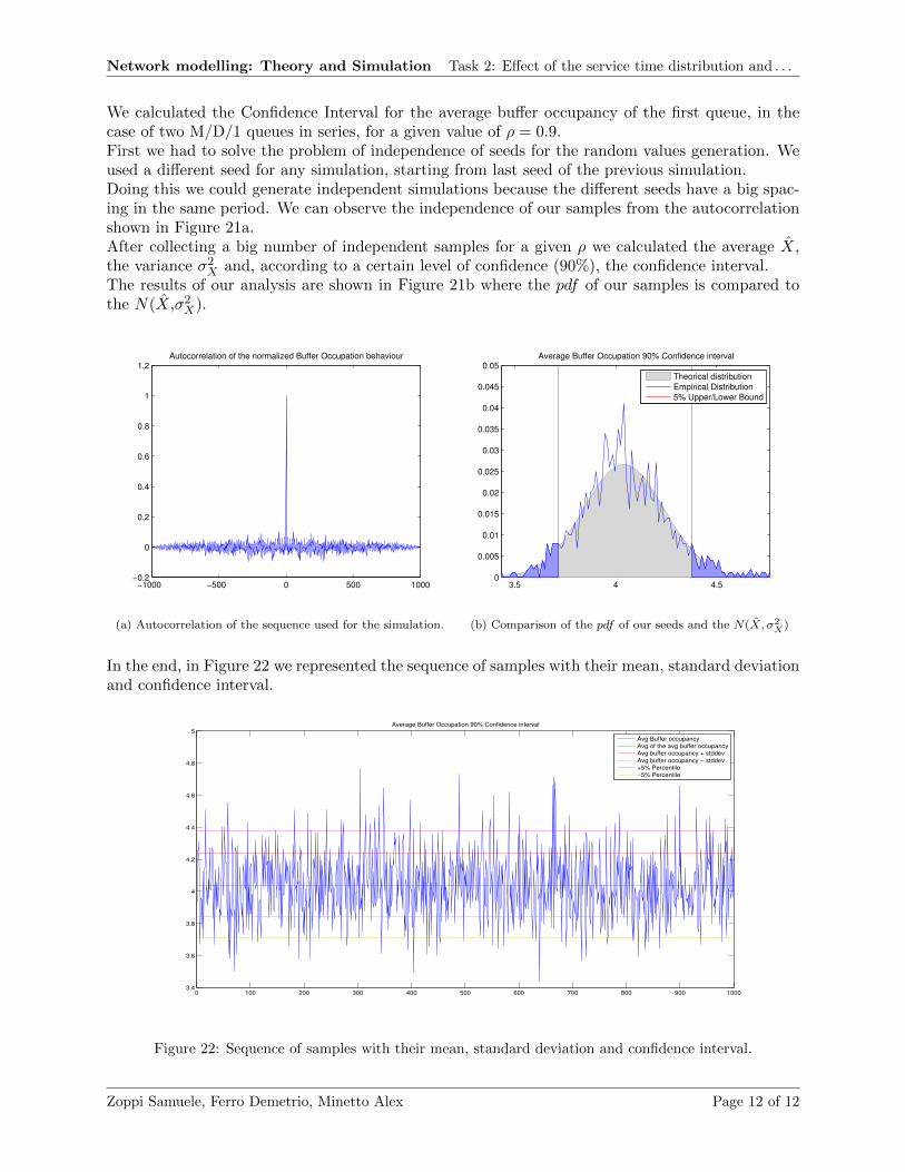
We calculated the Confidence Interval for the average buffer occupancy of the first queue, in thecase of two M/D/1 queues in series, for a given value of ρ = 0.9.First we had to solve the problem of independence of seeds for the random values generation. Weused a different seed for any simulation, starting from last seed of the previous simulation.Doing this we could generate independent simulations because the different seeds have a big spac-ing in the same period. We can observe the independence of our samples from the autocorrelationshown in Figure 21a.After collecting a big number of independent samples for a given ρ we calculated the average X̂,the variance σ2

X and, according to a certain level of confidence (90%), the confidence interval.The results of our analysis are shown in Figure 21b where the pdf of our samples is compared tothe N(X̂,σ2

X).

−1000 −500 0 500 1000−0.2

0

0.2

0.4

0.6

0.8

1

1.2Autocorrelation of the normalized Buffer Occupation behaviour

(a) Autocorrelation of the sequence used for the simulation.

3.5 4 4.50

0.005

0.01

0.015

0.02

0.025

0.03

0.035

0.04

0.045

0.05Average Buffer Occupation 90% Confidence interval

Theorical distribution

Empirical Distribution

5% Upper/Lower Bound

(b) Comparison of the pdf of our seeds and the N(X̂, σ2X)

In the end, in Figure 22 we represented the sequence of samples with their mean, standard deviationand confidence interval.

0 100 200 300 400 500 600 700 800 900 10003.4

3.6

3.8

4

4.2

4.4

4.6

4.8

5Average Buffer Occupation 90% Confidence interval

Avg Buffer occupancy

Avg of the avg buffer occupancy

Avg buffer occupancy + stddev

Avg buffer occupancy − stddev

+5% Percentile

−5% Percentile

Figure 22: Sequence of samples with their mean, standard deviation and confidence interval.


Report Network Modelling

Science

Transcript of Report Network Modelling