Learning Directed Probabilistic Logical

Models: Ordering-Search versus

Structure-Search

Daan Fierens

Jan Ramon

Maurice Bruynooghe

Hendrik Blockeel

Report CW490, May 2007

Katholieke Universiteit LeuvenDepartment of Computer Science

Celestijnenlaan 200A – B-3001 Heverlee (Belgium)

Learning Directed Probabilistic Logical

Models: Ordering-Search versus

Structure-Search

Daan Fierens

Jan Ramon

Maurice Bruynooghe

Hendrik Blockeel

Report CW490, May 2007

Department of Computer Science, K.U.Leuven

Abstract

There is an increasing interest in upgrading Bayesian networksto the relational case, resulting in so-called directed probabilisticlogical models. In this paper we discuss how to learn non-recursivedirected probabilistic logical models from relational data. This prob-lem has already been tackled before by upgrading the structure-search algorithm for learning Bayesian networks. In this paper wepropose to upgrade another algorithm, namely ordering-search, sincefor Bayesian networks this was found to work better than structure-search. We experimentally compare the two upgraded algorithms ontwo relational domains.

Keywords : Statistical Relational Learning, Probabilistic Logical Models, In-ductive Logic Programming, Bayesian Networks, Probability Trees, DtructureLearningCR Subject Classification : I.2.6

1

1 Introduction

There is an increasing interest in probabilistic logical models as can be seen from thevariety of formalisms that have recently been introduced for describing such models.Many of these formalisms deal with directed models that are upgrades of Bayesian net-works to the relational case. Learning algorithms have been developed for several suchformalisms [9, 12, 15]. Most of these algorithms are essentially upgrades of the tradi-tional structure-search algorithm for Bayesian networks [10]. In 2005, an alternativealgorithm for learning Bayesian networks was introduced: ordering-search. This wasfound to perform at least as good as structure-search while usually being faster. Thismotivates us to investigate how ordering-search can be upgraded to the relational case.

The contributions of this work are two-fold. First, we upgrade the ordering-searchalgorithm towards learning non-recursive directed probabilistic logical models. Second,we experimentally compare the resulting algorithm with the upgraded structure-searchalgorithm on two relational domains. We use the formalism Logical Bayesian Networks[5] but the proposed approach is also valid for related formalisms such as ProbabilisticRelational Models [8, 9], Bayesian Logic Programs [12, 13] and Relational BayesianNetworks [11]. Part of this work has been published before [6].

This paper is structured as follows. We review Logical Bayesian Networks in Sec-tion 2. We discuss the setting of learning non-recursive Logical Bayesian Networks inSection 3 and various learning algorithms in Section 4. We experimentally comparethese algorithms in Section 5. In Section 6 we briefly discuss learning in the recursivecase. Finally, in Section 7 we conclude.

2 Logical Bayesian Networks

We first discuss some preliminaries. Then we review Logical Bayesian Networks bymeans of an example. Then we briefly discuss the existence of syntactic variants ofLogical Bayesian Networks. Finally, we define the notion of non-recursive LogicalBayesian Networks.

2.1 Preliminaries: Bayesian Networks and Logic Programming

A Bayesian network is a compact specification of a joint probability distribution on aset of random variables under the form of a directed acyclic graph (the structure) and aset of conditional probability distributions (CPDs). When learning from data the goal isusually to find the structure and CPDs that maximize a certain scoring criterion (suchas likelihood or the Bayesian Information Criterion [10]).

Logical Bayesian Networks share some terminology with logic programming. Apredicate represents a property or relation and is denoted as p/n, where p is the nameand n is the number of arguments or arity, for example student/1. Arguments can beconstants (denoted by lower-case symbols), variables (denoted by upper-case symbols)or compound objects (not considered further). An atom is a predicate together with theright number of arguments, for example student(tim) or student(S). A literal is anatom or a negated atom, for example not(student(john)). A ground atom or literal is

2

an atom or literal that does not contain any variables as arguments. An interpretation ofa set of logical predicates is an assignment of a truth value to each ground atom that isbuilt from these predicates and that has arguments belonging to the considered domainof discourse (for example the considered set of people).

2.2 Logical Bayesian Networks: Example

A Logical Bayesian Network or LBN [5] is essentially a specification of a Bayesian net-work conditioned on some logical input predicates describing the domain of discourse.For instance, when modelling the well-known ‘university’ domain [9], we would usepredicates student/1, course/1, prof/1, teaches/2 and takes/2 with their obviousmeanings. The semantics of an LBN is that, given an interpretation of these logicalpredicates, the LBN induces a particular Bayesian network.

In LBNs random variables are represented as ground atoms built from certain spe-cial predicates, the probabilistic predicates. For instance, if intelligence/1 is a prob-abilistic predicate then the atom intelligence(ann) is called a probabilistic atom andrepresents a random variable. Apart from sets of logical and probabilistic predicatesan LBN basically consists of three parts: a set of random variable declarations, a setof dependency clauses and a set of logical CPDs. The former two together determinethe structure of the induced Bayesian network, while the logical CPDs quantify thedependencies in this structure.

The Structure of the Induced Bayesian Networks For a given interpretation of thelogical predicates, the random variable declarations in an LBN determine the set of ran-dom variables (nodes) in the induced Bayesian network while the dependency clausesdetermine the dependencies (edges). Together, this fully determines the structure of theinduced Bayesian network. We now illustrate this with an example.

For the university domain, the random variable declarations are the following.

random(intelligence(S)) <- student(S).random(ranking(S)) <- student(S).random(difficulty(C)) <- course(C).random(rating(C)) <- course(C).random(ability(P)) <- prof(P).random(popularity(P)) <- prof(P).random(grade(S,C)) <- student(S),course(C),takes(S,C).random(satisfaction(S,C)) <- student(S),course(C),takes(S,C).

In these clauses random/1 is a special predicate. Informally, the first clause, for in-stance, should be read as “intelligence(S) is a random variable if S is a student”. For-mally, in the induced Bayesian network, there is a node for each ground probabilisticatom p for which random(p) holds.

The dependency clauses for the university domain are the following.

grade(S,C) | intelligence(S), difficulty(C).ranking(S) | grade(S,C).

3

satisfaction(S,C) | grade(S,C).satisfaction(S,C) | ability(P) <- teaches(P,C).rating(C) | satisfaction(S,C).popularity(P) | rating(C) <- teaches(P,C).

Informally, the first clause should be read as “the grade of a student S for a course Cdepends on the intelligence of S and the difficulty of C”. There are also more complexclauses such as the last clause, which should be read as “the popularity of a professorP depends on the rating of a course C if P teaches C”. In this clause, popularity(P )is called the head, rating(C) the body and teaches(P,C) the context. Formally, in theinduced Bayesian network there is an edge from a node pparent to a node pchild if thereis a ground instance of a dependency clause with pchild in the head, with pparent in thebody, with true context and with random(.) true for each probabilistic atom in the headand body.

Quantifying the Dependencies To quantify the dependencies specified by the de-pendency clauses, LBNs associate with each probabilistic predicate a so-called logicalCPD. These logical CPDs can be used to determine the CPDs in the induced Bayesiannetwork.

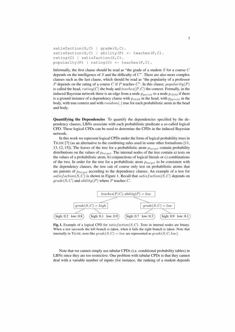
In this work we represent logical CPDs under the form of logical probability trees inTILDE [7] (as an alternative to the combining rules used in some other formalisms [11,13, 12, 15]). The leaves of the tree for a probabilistic atom ptarget contain probabilitydistributions on the values of ptarget. The internal nodes of the tree contain a) tests onthe values of a probabilistic atom, b) conjunctions of logical literals or c) combinationsof the two. In order for the tree for a probabilistic atom ptarget to be consistent withthe dependency clauses, the tree can of course only test on probabilistic atoms thatare parents of ptarget according to the dependency clauses. An example of a tree forsatisfaction(S,C) is shown in Figure 1. Recall that satisfaction(S,C) depends ongrade(S,C) and ability(P ) where P teaches C.

teaches(P, C), ability(P ) = low

grade(S, C) = high grade(S, C) = low

high: 0.2 low: 0.8 high: 0.1 low: 0.9 high: 0.7 low: 0.3 high: 0.9 low: 0.1

Fig. 1. Example of a logical CPD for satisfaction(S, C). Tests in internal nodes are binary.When a test succeeds the left branch is taken, when it fails the right branch is taken. Note thatinternally in TILDE, tests like grade(S, C) = low are represented as grade(S, C, low).

Note that we cannot simply use tabular CPDs (i.e. conditional probability tables) inLBNs since they are too restrictive. One problem with tabular CPDs is that they cannotdeal with a variable number of inputs (for instance, the ranking of a student depends

4

on his grades for all courses taken and the number of courses per student can vary).Logical probability trees in TILDE can deal with a variable number of inputs becausethe tests in the internal nodes can be first-order queries. As shown by Van Assche et al.[20], this makes it possible to express selection (for instance, does there exist a coursefor which the student has a high grade), aggregation (for instance, is the average of allgrades of the student high) and combinations of the two.

2.3 Equivalence of Sets of Dependency Clauses

Some LBNs have syntactic variants. The main manifestation of this is the fact that eachLBN that contains dependency clauses with multiple atoms in the body is equivalent toan LBN that contains only dependency clauses with one atom in the body (we explainthis below). Since syntactic variants could cause redundancy in the learning algorithm,they should be excluded as much as possible. Hence, when learning we only considerLBNs with dependency clauses with only one probabilistic atom in the body.

For each LBN with dependency clauses with multiple probabilistic atoms in thebody an equivalent LBN can be obtained by replacing each such dependency clause Cby a set of equivalent clauses. Concretely, for each probabilistic atom in the body of Cwe create a new clause with the same head, with only that atom in the body and with ascontext the context of C plus the condition that all other probabilistic atoms in the bodyof C are random variables. Rather than formally proving that this yields an equivalentLBN, we illustrate this with two examples.

Example 1 Consider the university domain from the previous section. The LBN for thisdomain contains one dependency clauses with multiple atoms in the body, namely thefollowing clause.

grade(S,C) | intelligence(S), difficulty(C).

Following the definition of dependency clauses, the dependency of grade on intelligenceand on difficulty only holds for student-course pairs for which intelligence and difficultyare defined (i.e. are random variables). Hence, this clause can be replaced by the fol-lowing set of equivalent clauses.

grade(S,C) | intelligence(S) <- random(difficulty(C)).grade(S,C) | difficulty(C) <- random(intelligence(S)).

We can simplify these clauses by using the information provided by the random variabledeclarations. First we can replace the random(.) literals in the context of the clausesby their definitions. This yields the following clauses.

grade(S,C) | intelligence(S) <- course(C).grade(S,C) | difficulty(C) <- student(S).

The random variable declarations can be used to simplify these clauses even further.The condition course(C) in the context of the first clause can be dropped since grade(S,C)is only defined if C is a course anyway. Similarly, the condition student(S) in the con-text of the second clause can be dropped. We finally obtain the following clauses.

5

grade(S,C) | intelligence(S).grade(S,C) | difficulty(C).

Example 2 As a more advanced example, consider the following LBN.

random(ranking(S)) <- student(S).random(intelligence(S)) <- student(S).random(thesis_score(S)) <- student(S), in_master(S).ranking(S) | intelligence(S), thesis_score(S).

Note that ranking and intelligence are defined for students but thesis-score is definedonly for particular students, namely master students. Following the definition of depen-dency clauses, the dependency of ranking on intelligence and thesis-score only holds forstudents for which both intelligence and thesis-score are defined. In other words, the de-pendency only holds for master students. This dependency clause can be replaced bythe following set of equivalent clauses.

ranking(S) | intelligence(S) <- random(thesis_score(S)).ranking(S) | thesis_score(S) <- random(intelligence(S)).

As in the previous example, we can again simplify these clauses by using the randomvariable declarations. After the first step we get the following clauses.

ranking(S) | intelligence(S) <- student(S), in_master(S).ranking(S) | thesis_score(S) <- student(S).

In the second step the condition student(S) in the context of both clauses can bedropped since ranking is only defined for students. We finally obtain the followingclauses.

ranking(S) | intelligence(S) <- in_master(S).ranking(S) | thesis_score(S).

Note that the second clause does not specify in the context that S should be a masterstudent. This is indeed not needed since thesis-score is only defined for master studentsand hence the clause only applies to master students anyway.

2.4 Recursive and Non-recursive Logical Bayesian Networks

The predicate dependency graph of an LBN is the graph that contains a node for eachprobabilistic predicate and an edge from a node p1 to a node p2 if the LBN contains adependency clause with predicate p2 in the head and p1 in the body.

An LBN is called non-recursive if its predicate dependency graph is acyclic andrecursive otherwise. Note that for non-recursive LBNs the induced Bayesian network(for any interpretation of the logical predicates) is always acyclic.

6

3 Learning Non-recursive Logical Bayesian Networks: TheLearning Setting

We now discuss the problem of learning LBNs from relational data. In the learningsetting that we consider, the random variable declarations are given (this is similar tothe setting for Probabilistic Relational Models where the relational schema is given[8, 9]). The goal of learning is to find the dependency clauses and logical CPDs thatmaximize the scoring criterion. We focus on learning non-recursive LBNs. We brieflydiscuss learning recursive models in Section 6.

We assume that we have a dataset of mega examples (terminology adapted fromMihalkova et al. [14]). Each mega example is a set of connected pieces of information.For instance, in a dataset about the inheritance of genes among family members, eachmega example would correspond to one particular family; in a dataset for the universitydomain, each mega example corresponds to one particular collection of students, pro-fessors and courses with their relations and properties. We assume that mega examplesare mutually independent. Learning from a dataset consisting of independent mega ex-amples (as opposed to learning from a single relational database) is useful for instancefor cross validation. We use the term ‘mega example’ rather than simply ‘example’because, as we will see later, each mega example can give rise to multiple smaller ex-amples for learning logical CPDs.

In our learning setting, each mega example consists of two parts: a logical part and aprobabilistic part. The logical part consists of an interpretation of the logical predicates.The probabilistic part consists of an assignment of values to all ground random variables(as determined by the random variable declarations). This is similar to the data used forlearning Bayesian Logic Programs [4] and Relational Bayesian Networks [11].

Example 3 Consider a simplified variant of the university domain in which we consideronly students and courses (but no professors) and use only four probabilistic predicates(ranking/1, difficulty/1, rating/1 and grade/2). The logical part of a mega examplewould then specify all students and courses and which students take which courses inthat mega example. This could for instance look as follows.

student(s1). student(s2).course(c1). course(c2).takes(s1,c1). takes(s2,c1). takes(s2,c2).

The probabilistic part of a mega example specifies a value for all random variables forthat mega example. This could for instance look as follows.

ranking(s1)=high ranking(s2)=middifficulty(c1)=mid difficulty(c2)=highrating(c1)=low rating(c2)=midgrade(s1,c1)=high grade(s2,c1)=mid grade(s2,c2)=low

7

4 Learning Non-recursive Logical Bayesian Networks: TheAlgorithms

We first briefly discuss a generic algorithm for learning the structure of LBNs in Sec-tion 4.1. In Section 4.2 we discuss how to learn logical CPDs under the form of logicalprobability trees. In Sections 4.3 and 4.4 we give two instantiations of the generic al-gorithm for learning LBNs. The first is the upgraded ordering-search algorithm that weintroduce in this paper. The second is the existing upgraded structure-search algorithm.To stress the difference with Logical Bayesian Networks we will sometimes refer toordinary Bayesian networks as ‘propositional’ Bayesian networks.

4.1 A Generic Algorithm for Learning Logical Bayesian Networks

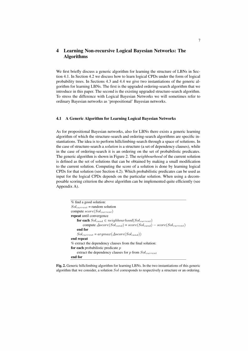
As for propositional Bayesian networks, also for LBNs there exists a generic learningalgorithm of which the structure-search and ordering-search algorithms are specific in-stantiations. The idea is to perform hillclimbing-search through a space of solutions. Inthe case of structure-search a solution is a structure (a set of dependency clauses), whilein the case of ordering-search it is an ordering on the set of probabilistic predicates.The generic algorithm is shown in Figure 2. The neighbourhood of the current solutionis defined as the set of solutions that can be obtained by making a small modificationto the current solution. Computing the score of a solution is done by learning logicalCPDs for that solution (see Section 4.2). Which probabilistic predicates can be used asinput for the logical CPDs depends on the particular solution. When using a decom-posable scoring criterion the above algorithm can be implemented quite efficiently (seeAppendix A).

% find a good solution:Solcurrent = random solutioncompute score(Solcurrent)repeat until convergence

for each Solcand ∈ neighbourhood(Solcurrent)compute ∆score(Solcand) = score(Solcand) − score(Solcurrent)

end forSolcurrent = argmax(∆score(Solcand))

end repeat% extract the dependency clauses from the final solution:for each probabilistic predicate p

extract the dependency clauses for p from Solcurrent

end for

Fig. 2. Generic hillclimbing algorithm for learning LBNs. In the two instantiations of this genericalgorithm that we consider, a solution Sol corresponds to respectively a structure or an ordering.

8

To use the generic algorithm of Figure 2 with a specific kind of solutions (structures,orderings, . . . ) one has to determine a) how to obtain an initial random solution1, b) howto define the neighbourhood of a solution, c) how to learn and score logical CPDs, andd) how to extract the dependency clauses from the learned solution. We explain learninglogical CPDs in Section 4.2. We explain each of the other issues for ordering-search inSection 4.3 and for structure-search in Section 4.4.

4.2 Learning Logical CPDs

Logical CPDs represented as logical probability trees (such as the tree in Figure 1) canbe learned using any of the standard probability tree algorithms in TILDE [7]. Belowwe discuss the data needed for learning such trees and the scoring criteria that we used.

Data for Learning Logical CPDs To learn a logical CPD for a target predicate ptarget

we need a dataset of labelled examples which can be derived from the mega examplesin the original dataset. In general, a single mega example can give rise to multipleexamples in the dataset for the logical CPD since there can be multiple ground atomsfor the predicate ptarget in the mega example. Concretely, each random variable (groundprobabilistic atom) R built from ptarget in each mega example m leads to one examplee in the dataset for the logical CPD. This example e is labelled with the value of R inm and consists of the part of m that is relevant for R.

Example 4 Consider the logical CPD for the probabilistic predicate difficulty/1 in theuniversity domain. Note that each random variable for difficulty/1 in each mega exam-ple corresponds to a particular course. Hence, each course C in each mega example mgives rise to another example e in the dataset for this logical CPD. Such an example econtains all information from the mega example m that is about the course C or abouta student linked to C (for instance through the takes relationships).

Concretely, the simplified mega example given in Example 3 contains two coursesand hence leads to two examples in the dataset for the logical CPD for difficulty/1. Thefirst example is about course c1, is labelled with ‘difficulty=mid’ and looks as follows.

course(c1).student(s1). student(s2).takes(s1,c1). takes(s2,c1).

ranking(s1)=high ranking(s2)=midrating(c1)=lowgrade(s1,c1)=high grade(s2,c1)=mid

The second example is about course c2, is labelled with ‘difficulty=high’ and looks asfollows.

1 The initial solution might influence the final result since the algorithm only converges to a localoptimum. Hence, we experimented with random restarts (multiple runs with different initialrandom solutions) but we found this not to be significantly better than a single run.

9

course(c2).student(s2).takes(s2,c2).

ranking(s2)=midrating(c2)=midgrade(s2,c2)=low

Scoring Criteria In this paper we consider two ways of learning and scoring trees.A straightforward approach is to learn and score trees using the Bayesian InformationCriterion (BIC) [7, 10]. We also looked for an alternative approach since BIC is knownto perform poorly when the cardinality (number of possible values) of the random vari-ables is rather high. In this alternative approach we learn trees using randomizationtest pruning [7] since this works well even when the cardinality is high. However, ran-domization is a pruning criterion that can only be used to learn trees but not to scorethem. Of course, we cannot use BIC to score the trees learned using randomizationsince this would not solve our original problem. As a simple solution, we instead uselog-likelihood as a scoring criterion, although this has the drawback of not penalizingextra dependency clauses which could potentially lead to overfitting. We refer to thisalternative approach as “randomization/likelihood”.

4.3 Ordering-search

We now discuss ordering-search. First we briefly discuss the propositional case. thenwe discuss the case of LBNs and the differences between the two.

Ordering-search for Propositional Bayesian Networks Ordering-search is based onthe fact that it is relatively easy to learn a Bayesian network if an ordering on the setof random variables is given [19]. Such an ordering eliminates the possibility of cycles.This makes it possible to decide for each variable X separately which variables, fromall variables preceding it in the ordering, are its parents. This can simply be done bylearning a CPD for X under the assumption that ‘selective’ CPDs are used , i.e. CPDsthat select from all candidate inputs the relevant inputs (for instance conditional prob-ability tables with a bound on the number of effective inputs [19]). However, the scoreof the Bayesian network that is learned in this way depends heavily on the quality ofthe ordering that is used. Hence, the idea of ordering-search is to perform hillclimbingthrough the space of possible orderings, in each step applying the above procedure.

Teyssier and Koller [19] experimentally compared ordering-search to structure-search for propositional Bayesian networks and found that ordering-search is alwaysat least as good and usually faster. As an explanation they note that the space of or-derings is smaller than the space of structures and that ordering-search does not needcostly acyclicity checks.

Ordering-search for Logical Bayesian Networks Until now ordering-search has notyet been upgraded to the case of non-recursive directed probabilistic logical models.

10

The above conclusions from the propositional case motivated us to investigate this up-grade. We now show how to upgrade ordering-search towards learning non-recursiveLBNs.

Similar to the case of propositional Bayesian networks, it is easy to learn a non-recursive LBN when an ordering on the set of probabilistic predicates is given. Wecan then learn an LBN simply by learning for each probabilistic predicate p a logicalprobability tree with as inputs all predicates preceding p in the ordering. Ordering-search corresponds to applying the generic algorithm of Figure 2 with orderings assolutions. This is basically hillclimbing through the space of orderings. As an initialordering we use any random ordering. The score of an ordering is defined as the scoreof the LBN that is learned for that ordering. The neighbourhood of an ordering O isdefined as the set of orderings that can be obtained by swapping a pair of adjacentpredicates in O (this is similar to what is done for propositional Bayesian networks[19]). Note that this implies that the size of the neighbourhood is linear in the numberof probabilistic predicates. Once we found the optimal ordering and the logical CPDsfor this ordering, we still need to extract the dependency clauses from these logicalCPDs. We now discuss this in more detail.

Extracting the Dependency Clauses from the Logical CPDs Below we explain howto extract the dependency clauses from a logical probability tree. To obtain an LBN,this procedure has to be applied to the probability tree for each probabilistic predicate.

When extracting dependency clauses from a logical probability tree with as targetthe probabilistic atom ptarget, we want to find the most specific set of clauses that isconsistent with the tree. With consistent we mean that the tree should never test anyprobabilistic atom that is not a parent of ptarget according to the set of clauses.

When extracting dependency clauses from a tree, we create a clause for each test ona probabilistic atom in each internal node of the tree. Call the atom that is tested ptest

and the node N . In the most general case, apart from the test on ptest, the node N cancontain a number of tests on other probabilistic atoms and a conjunction l of logicalliterals. We then create a dependency clause of the form ptarget | ptest ← l, path(N),where path(N) is a conjunction of logical literals that describes the path from the rootto N . Each node on this path can contribute a number of logical literals to path(N).A succeeded node (i.e. a node for which the succeeding branch of the tree was chosenin the path) contributes all logical literals that it contains. A failed node that does notcontain any tests on probabilistic atoms contributes the negation of all its logical literals.A failed node that contains a test on a probabilistic atom does not contribute to the path(letting such a node contribute the negation of its logical literals could be inconsistentsince we cannot be sure that it were the logical literals that caused the failure and notthe probabilistic tests).

Example 5 Consider the probability tree shown in Figure 1. For this tree, ptarget issatisfaction(S,C). For the root node, ptest is ability(P ), l is teaches(P,C) and thepath is empty. For the internal node below the root to the left, ptest is grade(S,C), lis empty and the path is teaches(P,C). For the node below the root to the right, ptest

is grade(S,C) and l and the path are both empty. The three resulting clauses for thesenodes are respectively the following.

11

satisfaction(S,C) | ability(P) <- teaches(P,C).satisfaction(S,C) | grade(S,C) <- teaches(P,C).satisfaction(S,C) | grade(S,C).

Note that in principle the second clause can be dropped (it is a special case of the third).However, such a form of post-processing is currently not implemented in our learningsystem.

Note that in the above procedure for extracting the dependency clauses from a log-ical probability tree, the probabilistic atoms in the internal nodes never contribute topath(N) for a node N . The reason for this is that the context of a dependency clause isnot allowed to contain probabilistic atoms. This implies that generally not all indepen-dence information specified in a logical probability tree can be captured by the depen-dency clauses. This is of course not surprising since this also holds in the propositionalcase (for instance, a CPD under the form of a probability tree can capture context-specific independence while the structure of a Bayesian network cannot [3]).

Differences between Ordering-search for LBNs and Propositional Ordering-searchTwo obvious differences between ordering-search for LBNs and ordering-search as pro-posed by Teyssier and Koller [19] for propositional Bayesian networks are that forLBNs we use orderings on the set of probabilistic predicates (instead of on the setof random variables) and the extraction of the structure from the CPDs is more com-plex. A third and more important difference is that we use logical probability trees asCPDs whereas Teyssier and Koller use tabular CPDs. Recall that for LBNs we cannotuse simple tabular CPDs since they are too restrictive (see Section 2.2). However, forpropositional Bayesian networks it would be possible to use (propositional) probabilitytrees instead of tabular CPDs. Such an approach would have both an advantage and adisadvantage with respect to efficiency.

The advantage of using probability trees instead of tabular CPDs is that the effectiveparents of a random variable X can then be determined from the set of candidate parentsof X (i.e. all variables preceding X in the current ordering) by learning only a singleCPD for X . This is because probability trees are selective, so we can simply learn a treeusing all candidate parents as input and determine the effective parents as all randomvariables that are used in the learned tree. In contrast, tabular CPDs are not selective.Hence, the approach of Teyssier and Koller is to put an upper bound k on the number ofinputs for the CPDs; the lower k, the more selective the approach is. Teyssier and Kollercompute the score of all CPDs for X having at most k candidate parents as inputs andthen determine the effective parents as all random variables that are used in the highestscoring CPD for X . Of course, this is only feasible for small k (Teyssier and Koller useat most k = 4).

The disadvantage of using probability trees instead of tabular CPDs is that a tabularCPD can be learned more efficiently than a probability tree, especially if the number ofinputs for the CPD is bounded by a small number k. This allows Teyssier and Kollerto compute beforehand the sufficient statistics for all CPDs that could ever be neededduring the search over orderings. As a consequence, the actual search over orderingsbecomes very fast. In contrast, when using probability trees it is not efficient to learn all

12

CPDs beforehand. Hence, in our ordering-search algorithm for LBNs we do not learnprobability trees beforehand but learn them on the fly as they are needed.

To the best of our knowledge, ordering-search for propositional Bayesian networkshas not yet been used with probability trees. Hence, it is unclear whether the aboveadvantage of probability trees over tabular CPDs outweighs its disadvantage or viceversa. Note, however, that this issue is only relevant in the propositional case and not inthe case of LBNs since there tabular CPDs are too restrictive.

4.4 Structure-search

Structure-search (also known as DAG-search) is the most traditional and most straight-forward approach for learning propositional Bayesian networks [10]. It is essentiallyhillclimbing through the space of possible structures. The neighbourhood of the cur-rent structure typically consists of all acyclic structures that can be obtained by adding,deleting or reversing an edge. This algorithm has already been upgraded to the rela-tional case for several formalisms [8, 9, 12, 13, 15]. The algorithm that we use for LBNsis very similar to these existing upgrades.

To derive a concrete structure-search algorithm for LBNs from the generic algo-rithm of Figure 2, we have to define the notion of a neighbourhood and define how aninitial structure is obtained (note that for structure-search the final step in the genericalgorithm, extracting clauses from the solution, is not needed since a solution is a setof dependency clauses). We define the neighbourhood of the current structure as theset of all non-recursive structures that can be obtained by adding a dependency clause,deleting a clause or swapping the head and body of a clause in the current structure.Note that this implies that the size of the neighbourhood is quadratic in the numberof probabilistic predicates. To find an initial set of clauses we borrow some elementsfrom the ordering-search algorithm. Specifically, we generate a random initial ordering,learn logical CPDs for this ordering and apply the procedure for extracting dependencyclauses from logical CPDs. In our experiments, we use the same random initial orderingfor ordering-search and structure-search. Hence, both algorithms always start from thesame point. This ensures that an experimental comparison of both algorithms evaluatesthe search process itself and not the starting point of the search.

We implemented one extension to the above structure-search algorithm for LBNs:lookahead. When using lookahead we not only try adding one clause but also addingtwo clauses with the same head during a single refinement step. This is useful whenadding only one of the two clauses does not change the score, which is the case whenthe parent introduced by one clause is not predictive for the head in itself but onlytogether with the parent introduced by the other clause. In the propositional case, thishappens for instance when the head is the XOR of both parents. In the relational case,this happens for instance when the function of one predicate inside the logical CPD forthe head is only to introduce a new logical variable used by another predicate in thelogical CPD (this is a standard case of lookahead in inductive logic programming [1,16]). Of course, in order for lookahead at the level of dependency clauses to have aneffect, lookahead also needs to be applied at the level of logical CPDs. In our case thismeans that the logical probability trees should be learned using lookahead [1].

13

5 Experiments

We first discuss the datasets used and the experimental setup. Then we discuss ourexperimental results: first we compare ordering-search to structure-search, next we an-alyze runtimes of both algorithms and finally we briefly investigate the influence of thescoring criterion.

5.1 Datasets

We perform experiments on two relational domains: the synthetic university domainand the real-world UWCSE dataset.

For the synthetic university domain we generated datasets with a varying numberof mega examples from the LBN given in Section 2. The logical part of each mega ex-ample was specified by hand (it contains 20 students, 10 courses, 5 professors and theirrelationships). The probabilistic part of each mega example was constructed by sam-pling from the given LBN. Each mega example corresponds to 230 random variables.We used datasets of 5, 10, 15, 31, 62, 125 and 250 mega examples.

The UWCSE dataset is a real-world dataset that is currently a popular benchmark inthe field of statistical relational learning [18]. This dataset was constructed by extract-ing information about graduate students, professors and courses from the web pages ofa computer science department. The dataset consists of 5 mega examples, each cor-responding to a specific research area. Since in this dataset relations are of specialimportance2, we decided to incorporate them into the probabilistic model, leading towhat Getoor et al. call relational uncertainty [9]. In LBNs this can be accomplishedby simply modelling the relations as probabilistic predicates. We only used four logi-cal predicates: student/1, prof/1, course/1 and same area/2. The random variabledeclarations look as follows.

random(phase_in_PhD(S)) <- student(S).random(year_in_PhD(S)) <- student(S).random(nb_publications(S)) <- student(S).random(position(P)) <- prof(P).random(nb_publications(P)) <- prof(P).random(level(C)) <- course(C).random(teaches(P,C)) <- prof(P),course(C),same_area(P,C).random(assistant(S,C)) <- student(S),course(C),same_area(S,C).random(advised_by(S,P)) <- student(S),prof(P),same_area(S,P).random(co_author(S,P)) <- student(S),prof(P),same_area(S,P).

In total the dataset contains 140 students, 132 courses and 52 professors, leading to9607 random variables. Of course, since this is a real-world dataset the true dependencyclauses are unknown.

2 For instance, this dataset has been used for supervised learning with the ‘advised by’ relationas the target [18].

14

5.2 Experimental Setup

For all experiments we performed 5-fold cross validation. For the synthetic universitydomain, mega examples were divided over folds randomly. For UWCSE, each foldcorresponds to one mega example. We report the average results over the folds and usetwo-tailed paired t-tests (with α=0.05) to assess the significance of differences betweentwo algorithms.

We use four evaluation criteria: normalized test log-likelihood (the log-likelihoodon the test data divided by the number of mega examples), normalized train score (thescore on the training data divided by the number of mega examples; while not impor-tant in itself it can give some insight into the degree of overfitting of an algorithm),number of dependency clauses learned (smaller is usually better because of ease ofinterpretation) and runtime.

For the synthetic university domain we know the true LBN that generated the data.Hence, we can use as a fifth evaluation criterion the degree to which the learned LBNsmatches this true LBN. A simple measure for this degree of overlap would be the num-ber of dependency clauses in the true LBN that are also in the learned LBN. However,the problem with this is that it is in general not possible to learn the true direction (whichatom is in the head and which in the body) of each dependency clause from data. This issimilar to the case of propositional Bayesian networks. The reason for this is that eachBayesian network has a Markov equivalence class, which is a set of networks that allhave the same score but different directions for some of the edges [2]. Hence, insteadof directly comparing the learned LBN and the true LBN, we measure the overlap be-tween the Markov equivalence class of the learned LBN and the true LBN. We do thisby finding the LBN in the equivalence class of the learned LBN which has the mostdirected edges in common with the true LBN. We refer to this number as the number ofcorrect dependencies learned.

For all evaluation criteria we report the results for the various algorithms. For testlog-likelihood and train score we additionally report the results for the ‘empty LBN’ asa baseline. With an ‘empty LBN’ we mean an LBN with no dependency clauses, thisis the LBN according to which all random variables are independent. We report resultsboth with BIC as a scoring criterion and with randomization/likelihood.

In the following sections we only give summaries of our experimental results. Thefull results are given in Appendix B.

5.3 Ordering-search versus Structure-search

We now discuss the results of our experimental comparison of ordering-search andstructure-search. We first discuss our results on the synthetic university domain andthen our results on the UWCSE dataset.

The Synthetic University Domain We tried two algorithms on the datasets for thisdomain: ordering-search (OS) and structure-search without lookahead (SS). We did nottry structure-search with lookahead on these datasets since lookahead is not needed tolearn the target LBN for this domain (there are no probabilistic predicates whose onlyfunction is to introduce a new logical variable).

15

The results are summarised in Table 1. An entry in this table (for a particular evalu-ation criterion and dataset size) has the following meaning: if one of the two algorithms(OS or SS) is significantly better than the other we show the best algorithm; if there isno statistically significant difference between the two algorithms we fill in “/”. We alsoplotted the results as a function of dataset size in Figure 3 (we only show the resultswith BIC as a scoring criterion since the results with randomization/likelihood lookvery similar).

Table 1. Significance of differences between results of OS and of SS on synthetic universitydatasets of varying size (upper half of table: BIC; lower half: randomization). Both OS and SShave significantly better test log-likelihood and train score than the empty LBN in all cases (thisis not shown in the table).

#MegaEx (#Vars) LogLik(Test) Score(Train) #Clauses #CorrectDepend Time5 (1150) / / / / OS10 (2300) / / / / OS15 (3450) / / / / OS31 (7130) / / / / OS62 (14260) / / / / OS125 (28750) / / / SS OS250 (57500) / / / SS OS

5 (1150) / SS OS / OS10 (2300) / / OS / OS15 (3450) / SS / / OS31 (7130) / / / SS OS62 (14260) / / / / OS125 (28750) / SS OS / OS250 (57500) / / / / OS

We can see from Table 1 that the results for test log-likelihood and runtime are con-sistent over various datasets sizes and scoring criteria (BIC or randomization/likelihood).The results for the number of dependency clauses and the number of correct dependen-cies learned are less clear.

OS and SS always obtain significantly better test log-likelihood and train score thanthe empty LBN. Table 1 shows that SS in some cases obtains significantly better trainscore than OS but this does not carry over to the test data: there is never a significant dif-ference in test log-likelihood between OS and SS. The evolution of test log-likelihoodand train score as a function of the dataset size (Figure 3) is as expected: both improverapidly when initially increasing the dataset size but this improvement slows down whenmoving to bigger datasets and likelihood and score seem to saturate. The figure alsoshows that the differences between OS and SS are small as compared to the differenceswith the empty LBN.

The results for the number of dependency clauses are not very clear. OS learnssignificantly less clauses than SS (i.e. learns more compact models) on three cases with

16

-1.5

-1.45

-1.4

-1.35

-1.3

-1.25te

stlo

g-lik

.

0 50 100 150 200 250-1.5

-1.45

-1.4

-1.35

-1.3

-1.25

trai

nsc

ore

0 50 100 150 200 250

0

4

8

12

#cl

ause

s

0 50 100 150 200 2500

2

4

6

#co

rrde

pend

enci

es

0 50 100 150 200 250

number of mega examples

0

200

400

600

time

(s)

0 50 100 150 200 250

number of mega examples

10

20

30

40

50

60

70

80

90

100

10 20 30 40 50 60 70 80 90 100

Legend:OSSSempty LBN

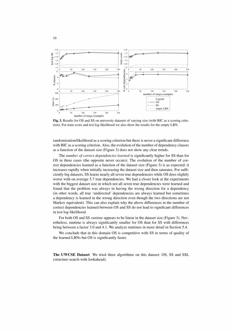
Fig. 3. Results for OS and SS on university datasets of varying size (with BIC as a scoring crite-rion). For train score and test log-likelihood we also show the results for the empty LBN.

randomization/likelihood as a scoring criterion but there is never a significant differencewith BIC as a scoring criterion. Also, the evolution of the number of dependency clausesas a function of the dataset size (Figure 3) does not show any clear trends.

The number of correct dependencies learned is significantly higher for SS than forOS in three cases (the opposite never occurs). The evolution of the number of cor-rect dependencies learned as a function of the dataset size (Figure 3) is as expected: itincreases rapidly when initially increasing the dataset size and then saturates. For suffi-ciently big datasets, SS learns nearly all seven true dependencies while OS does slightlyworse with on average 5.7 true dependencies. We had a closer look at the experimentswith the biggest dataset size in which not all seven true dependencies were learned andfound that the problem was always in having the wrong direction for a dependency(in other words, all true ‘undirected’ dependencies are always learned but sometimesa dependency is learned in the wrong direction even though the two directions are notMarkov equivalent). This can also explain why the above differences in the number ofcorrect dependencies learned between OS and SS do not lead to significant differencesin test log-likelihood.

For both OS and SS runtime appears to be linear in the dataset size (Figure 3). Nev-ertheless, runtime is always significantly smaller for OS than for SS with differencesbeing between a factor 3.0 and 4.1. We analyze runtimes in more detail in Section 5.4.

We conclude that in this domain OS is competitive with SS in terms of quality ofthe learned LBNs but OS is significantly faster.

The UWCSE Dataset We tried three algorithms on this dataset: OS, SS and SSL(structure-search with lookahead).

17

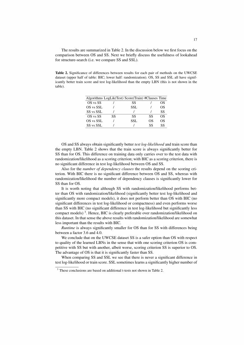
The results are summarized in Table 2. In the discussion below we first focus on thecomparison between OS and SS. Next we briefly discuss the usefulness of lookaheadfor structure-search (i.e. we compare SS and SSL).

Table 2. Significance of differences between results for each pair of methods on the UWCSEdataset (upper half of table: BIC; lower half: randomization). OS, SS and SSL all have signif-icantly better train score and test log-likelihood than the empty LBN (this is not shown in thetable).

Algorithms LogLik(Test) Score(Train) #Clauses TimeOS vs SS / SS / OS

OS vs SSL / SSL / OSSS vs SSL / / / SSOS vs SS SS SS SS OS

OS vs SSL / SSL OS OSSS vs SSL / / SS SS

OS and SS always obtain significantly better test log-likelihood and train score thanthe empty LBN. Table 2 shows that the train score is always significantly better forSS than for OS. This difference on training data only carries over to the test data withrandomization/likelihood as a scoring criterion; with BIC as a scoring criterion, there isno significant difference in test log-likelihood between OS and SS.

Also for the number of dependency clauses the results depend on the scoring cri-terion. With BIC there is no significant difference between OS and SS, whereas withrandomization/likelihood the number of dependency clauses is significantly lower forSS than for OS.

It is worth noting that although SS with randomization/likelihood performs bet-ter than OS with randomization/likelihood (significantly better test log-likelihood andsignificantly more compact models), it does not perform better than OS with BIC (nosignificant differences in test log-likelihood or compactness) and even performs worsethan SS with BIC (no significant difference in test log-likelihood but significantly lesscompact models) 3. Hence, BIC is clearly preferable over randomization/likelihood onthis dataset. In that sense the above results with randomization/likelihood are somewhatless important than the results with BIC.

Runtime is always significantly smaller for OS than for SS with differences beingbetween a factor 3.6 and 4.0.

We conclude that on the UWCSE dataset SS is a safer option than OS with respectto quality of the learned LBNs in the sense that with one scoring criterion OS is com-petitive with SS but with another, albeit worse, scoring criterion SS is superior to OS.The advantage of OS is that it is significantly faster than SS.

When comparing SS and SSL we see that there is never a significant difference intest log-likelihood or train score. SSL sometimes learns a significantly higher number of

3 These conclusions are based on additional t-tests not shown in Table 2.

18

dependency clauses (i.e. learns a significantly less compact model) while the oppositenever occurs. SSL is significantly slower than SS with differences being between afactor 1.9 and 2.4. Hence there is no reason to prefer SSL over SS so we conclude thatlookahead in structure-search has no added value on this dataset.

Finally, we investigated the learned LBNs to gain some more insight into this dataset.Most of the dependencies that were frequently learned (for the various algorithms andfolds) confirm our intuitions about this dataset. Some examples of such dependenciesand their common sense interpretations (obtained by investigating the correspondinglogical CPDs) are the following.

– phase in PhD(S) depends on year in PhD(S) (the logical CPD specified thata student is more likely to be in a later phase if he is in a higher year)

– nb publications(S) depends on year in PhD(S) (a student is more likely tohave many publications if he is in a higher year)

– nb publications(P ) depends on advised by(S, P ) (a professor is more likely tohave many publications if he advises more students)

– assistant(S,C) depends on advised by(S, P ) and teaches(P,C) (a student ismore likely to be the teaching assistant for a particular course if he is advised by aprofessor who teaches that course)

5.4 Analysis of Runtimes

In this section we analyze the runtime of the various algorithms in more detail by look-ing at the runtimes of the main different steps in the algorithms. Such an analysis hasnot been made before for ordering-search (also not for the propositional case).

The total runtime Ttotal of any concrete algorithm derived from the generic algo-rithm of Figure 2 can be decomposed as follows4

Ttotal = Tinit + Tfirst + Trest,

where Tinit denotes the initialization time (the time for learning and scoring all logicalCPDs for the initial random solution), Tfirst denotes the time for the first iteration (i.e.the first execution of the repeat loop in the generic algorithm) and Trest denotes thetime for all other iterations. The reason for considering the first iteration separately isthat it typically takes a lot longer than any of the other iterations (i.e. Tfirst > Tavg)since all the score-changes needed in the first iteration effectively have to be computed,while in the next iterations most of them can be reused without extra computation (seeAppendix A). Let I denote the number of iterations not including the first one. If wedefine the average time per iteration (not including the first one) as Tavg = Trest/I , wecan rewrite the total runtime as follows

Ttotal = Tinit + Tfirst + Tavg × I.

We now discuss our experimental results for each of the above measures. Note thatTinit is the same for all algorithms that we considered. Hence we only discuss Tfirst,Tavg and I . First we compare OS and SS, then we briefly compare SS and SSL.

4 The time needed for the final step of extracting the dependency clauses from the logical CPDscan be ignored since it is very small (it does not depend on the dataset size).

19

Recall from the previous section that in our experiments the total runtime Ttotal wasalways significantly lower for OS than for SS with differences being between a factor3.0 and 4.1. This can be explained as follows.

– The time for the first iteration, Tfirst, is always significantly lower for OS than forSS. This was expected since in the first iteration all elements of the neighbourhoodof the initial solution have to be scored and the size of the neighbourhood is smallerfor OS than for SS (linear in the number of probabilistic predicates for OS butquadratic for SS, see Section 4). In our experiments the difference in Tfirst betweenOS and SS goes from a factor 2.8 to 4.6.

– The average time per iteration (not including the first one), Tavg , is also alwayssignificantly lower for OS than for SS. This was expected for the same reasons asfor Tfirst above. In our experiments the difference in Tavg between OS and SSgoes from a factor 1.7 to 3.0.

– The conclusions about the number of iterations I are less clear: in 10 cases I issignificantly lower for OS than for SS, while in the remaining 6 cases there is nosignificant difference.

We now briefly discuss the influence of lookahead on the efficiency of structure-search. Recall from the previous section that in our experiments on the UWCSE datasetthe total runtime was always significantly higher for SSL than for SS. When analyzingruntimes we found that Tfirst and Tavg are always significantly higher for SSL than forSS. This was expected since the neighbourhood for SSL is bigger than for SS. However,we also found that the number of iterations is not significantly different for SSL thanfor SS. This was somewhat against our expectations. One would expect SSL to needless iterations than SS to convergence since SSL can take bigger steps in the searchspace (in a single step SSL can not only add one dependency clause but can also addtwo dependency clauses with the same head) but apparently this is not the case.

5.5 Influence of the Scoring Criterion

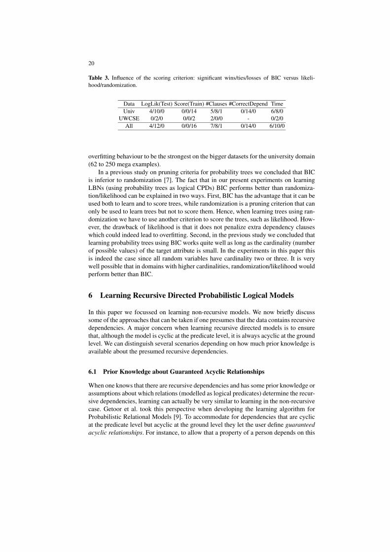
In this section we briefly compare the results for the two scoring criteria that we used:BIC and randomization/likelihood. The main results are summarized in Table 3. Thistable is based on all results for OS and SS (we left out SSL since we already concludedthat it does not have any advantages over SS). An entry like “5/8/1” in this table meansthat in 5 cases BIC is significantly better, in 8 cases there is no significant differenceand in 1 case randomization/likelihood is significantly better.

The main conclusion from Table 3 is that BIC is preferable over randomization/likeli-hood both in terms of test log-likelihood, number of dependency clauses learned andruntime. In fact it appears that randomization/likelihood overfits. This hypothesis isbased on two observations. First, although randomization/likelihood is always signifi-cantly better than BIC on training data, it is never significantly better and sometimessignificantly worse than BIC on test data. Second, randomization/likelihood often learnssignificantly more clauses than BIC while the number of correct clauses is never sig-nificantly higher than for BIC. In other words, the extra clauses learned by random-ization/likelihood are mainly redundant clauses. Upon closer inspection, we found this

20

Table 3. Influence of the scoring criterion: significant wins/ties/losses of BIC versus likeli-hood/randomization.

Data LogLik(Test) Score(Train) #Clauses #CorrectDepend TimeUniv 4/10/0 0/0/14 5/8/1 0/14/0 6/8/0

UWCSE 0/2/0 0/0/2 2/0/0 - 0/2/0All 4/12/0 0/0/16 7/8/1 0/14/0 6/10/0

overfitting behaviour to be the strongest on the bigger datasets for the university domain(62 to 250 mega examples).

In a previous study on pruning criteria for probability trees we concluded that BICis inferior to randomization [7]. The fact that in our present experiments on learningLBNs (using probability trees as logical CPDs) BIC performs better than randomiza-tion/likelihood can be explained in two ways. First, BIC has the advantage that it can beused both to learn and to score trees, while randomization is a pruning criterion that canonly be used to learn trees but not to score them. Hence, when learning trees using ran-domization we have to use another criterion to score the trees, such as likelihood. How-ever, the drawback of likelihood is that it does not penalize extra dependency clauseswhich could indeed lead to overfitting. Second, in the previous study we concluded thatlearning probability trees using BIC works quite well as long as the cardinality (numberof possible values) of the target attribute is small. In the experiments in this paper thisis indeed the case since all random variables have cardinality two or three. It is verywell possible that in domains with higher cardinalities, randomization/likelihood wouldperform better than BIC.

6 Learning Recursive Directed Probabilistic Logical Models

In this paper we focussed on learning non-recursive models. We now briefly discusssome of the approaches that can be taken if one presumes that the data contains recursivedependencies. A major concern when learning recursive directed models is to ensurethat, although the model is cyclic at the predicate level, it is always acyclic at the groundlevel. We can distinguish several scenarios depending on how much prior knowledge isavailable about the presumed recursive dependencies.

6.1 Prior Knowledge about Guaranteed Acyclic Relationships

When one knows that there are recursive dependencies and has some prior knowledge orassumptions about which relations (modelled as logical predicates) determine the recur-sive dependencies, learning can actually be very similar to learning in the non-recursivecase. Getoor et al. took this perspective when developing the learning algorithm forProbabilistic Relational Models [9]. To accommodate for dependencies that are cyclicat the predicate level but acyclic at the ground level they let the user define guaranteedacyclic relationships. For instance, to allow that a property of a person depends on this

21

property for his parents the parent relation has to be defined as guaranteed acyclic. Sim-ilarly, to allow that the topic of a paper depends on the topic of the papers publishedearlier by the same author, the published-earlier relation has to be defined as guaran-teed acyclic. Getoor et al. then apply structure-search and use the information aboutthe guaranteed acyclic relationships during the acyclicity checks to deduce that certaincycles at the predicate level are legal.

The algorithm of Getoor et al. is very similar to the structure-search algorithm usedfor LBNs in this paper. Hence the approach of using guaranteed acyclic relationshipscan be directly applied to our structure-search algorithm as well. Moreover, the sameapproach can also be applied to our ordering-search algorithm for LBNs. When learn-ing the logical CPD for a predicate p, the probabilistic predicates used as input wouldnot only be all predicates that precede p in the current ordering but also p itself and pos-sibly also all predicates following p in the ordering, with the restriction that p can onlydepend on itself and on the latter predicates through a guaranteed acyclic relationship.This actually requires no changes to our ordering-search algorithm but only requires toextend the declarative bias for the logical CPDs.

6.2 No Prior Knowledge

When one does not have enough prior knowledge about the data to find a set of guar-anteed acyclic relationships, more complicated approaches have to be taken. Whenapplying structure-search, one can use the techniques developed for Bayesian LogicPrograms [12, 13]. The idea is that the learning algorithm searches itself for the log-ical relations that determine the recursion and that acyclicity of a candidate model ischecked at the ground level for each example. The main drawback of this approach isthat the acyclicity checks might be computationally very expensive since the cost de-pends on the number of examples and the size of the examples. This is different fromthe non-recursive case where acyclicity of a candidate model only needs to be checkedonce and at the predicate level.

An alternative approach is to use generalized ordering-search [17], an algorithm werecently developed to learn recursive dependencies. Generalized ordering-search con-siders orderings on ground probabilistic atoms instead of on predicates (as the ordering-search algorithm proposed in this paper). In principle, generalized ordering-search canalso be used to learn non-recursive LBNs but in this respect it has a number of dis-advantages as compared to the algorithm proposed in this paper. One disadvantage isthat it does not learn an LBN ‘in closed form’: it does not learn a set of dependencyclauses but rather a procedural description of how to determine the induced Bayesiannetwork given any possible interpretation of the logical predicates. Another disadvan-tage is that it deviates quite far from the propositional ordering-search algorithm. Forinstance, when applied on propositional data generalized-ordering search does not cor-respond to the original propositional ordering-search algorithm, while this is the casefor the algorithm in this paper. This might make generalized-ordering search harder tounderstand for people familiar with the propositional ordering-search algorithm.

22

7 Conclusion

We upgraded the ordering-search algorithm for propositional Bayesian networks to-wards non-recursive directed probabilistic logical models. We experimentally comparedthe resulting algorithm with the existing upgraded structure-search algorithm on tworelational domains. The results show that ordering-search is competitive with structure-search in terms of quality of the learned models but is significantly faster than structure-search. We conclude that ordering-search is a good alternative to structure-search forlearning non-recursive directed probabilistic logical models.

Acknowledgements

Daan Fierens is supported by the Institute for the Promotion of Innovation by Scienceand Technology in Flanders (IWT Vlaanderen). Jan Ramon and Hendrik Blockeel arepost-doctoral fellows of the Research Foundation-Flanders (FWO Vlaanderen). Thisresearch is also supported by GOA 2003/08 “Inductive Knowledge Bases”.

References

1. H. Blockeel, and L. De Raedt. Lookahead and discretization in ILP. In Proceedings of the7th International Workshop on Inductive Logic Programming (ILP), volume 1297 of LectureNotes in Computer Science, pages 77–85. Springer Verlag, 1997.

2. D.M. Chickering. Learning equivalence classes of Bayesian network structures. Journal ofMachine Learning Research, volume 2, pages 445–498, 2002.

3. C. Boutilier, N. Friedman, M. Goldszmidt and D. Koller. Context-specific independence inBayesian networks. In Proceedings of the 12th conference on Uncertainty in AI (UAI), pages115–123. 1996.

4. L. De Raedt and K. Kersting. Probabilistic Inductive Logic Programming. In Proceedingsof the 15th International Conference on Algorithmic Learning Theory (ALT), volume 3244 ofLecture Notes in Computer Science, pages 19–36. Springer, 2004.

5. D. Fierens, H. Blockeel, M. Bruynooghe, and J. Ramon. Logical Bayesian networks and theirrelation to other probabilistic logical models. In Proceedings of the 15th International Con-ference on Inductive Logic Programming (ILP), volume 3625 of Lecture Notes in ComputerScience, pages 121–135. Springer, 2005.

6. D. Fierens, J. Ramon, M. Bruynooghe, and H. Blockeel. Learning Directed ProbabilisticLogical Models: Ordering-search versus Structure-search. In Proceedings of the 18th Euro-pean Conference on Machine Learning (ECML), volume 4701 of Lecture Notes in ComputerScience, Springer, 2007. To appear.

7. D. Fierens, J. Ramon, H. Blockeel, and M. Bruynooghe. A comparison of pruning criteriafor learning trees. Technical Report CW 488, Department of Computer Science, KatholiekeUniversiteit Leuven, April 2007.

8. N. Friedman, L. Getoor, D. Koller, and A. Pfeffer. Learning Probabilistic Relational Models.In Proceedings of the 16th International Joint Conference on Artificial Intelligence (IJCAI),pages 1300–1307, Morgan Kaufmann, 1999.

9. L. Getoor, N. Friedman, D. Koller, and A. Pfeffer. Learning Probabilistic Relational Models.In S. Dzeroski and N. Lavrac, editors, Relational Data Mining, pages 307–334. Springer-Verlag, 2001.

23

10. D. Heckerman, D. Geiger, and D.M. Chickering. Learning Bayesian networks: The com-bination of knowledge and statistical data. Machine Learning, volume 20, pages 197–243,1995.

11. M. Jaeger. Parameter learning for relational Bayesian networks. In Proceedings of the 24thInternational Conference on Machine Learning (ICML), 2007.

12. K. Kersting and L. De Raedt. Towards combining inductive logic programming and Bayesiannetworks. In Proceedings of the 11th International Conference on Inductive Logic Program-ming (ILP), volume 2157 of Lecture Notes in Computer Science, pages 118–131. Springer-Verlag, 2001.

13. K. Kersting and L. De Raedt. Basic principles of learning Bayesian logic programs. Techni-cal Report No. 174, Institute for Computer Science, University of Freiburg, June 2002.

14. L. Mihalkova, T. Huynh and R. Mooney. Mapping and revising Markov logic networks fortransfer learning. In Proceedings of the 22nd Conference on Artificial Intelligence (AAAI),2007.

15. S. Natarajan, W. Wong, and P. Tadepalli. Structure refinement in First Order ConditionalInfluence Language. In Proceedings of the ICML workshop on Open Problems in StatisticalRelational Learning (SRL), 2006.

16. R. Quinlan. Learning logical definitions from relations. Machine Learning, volume 5, pages239–266, 1990.

17. J. Ramon, T. Croonenborghs, D. Fierens, H. Blockeel, and M. Bruynooghe. Generalizedordering-search for learning directed probabilistic logical models. 2007. Conditionally ac-cepted for Machine Learning, special issue on Inductive Logic Programming.

18. M. Richardson and P. Domingos. Markov logic networks. Machine Learning, volume 62(1–2), pages 107–136, 2006.

19. M. Teyssier and D. Koller. Ordering-based search: A simple and effective algorithm forlearning Bayesian networks. In Proceedings of the 21st Conference on Uncertainty in AI(UAI), pages 584–590. AUAI Press, 2005.

20. A. Van Assche, C. Vens, H. Blockeel and S. Dzeroski. First order random forests: learningrelational classifiers with complex aggregates. Machine Learning, volume 64(1–3), pages149–182, 2006.

A Efficiently Implementing the Algorithms

In this appendix we briefly discuss how to efficiently implement ordering-search andstructure-search. The optimizations discussed below apply equally well to the proposi-tional case as to the case of LBNs. In fact, in the propositional case these optimizationsare standard [10].

A decomposable scoring criterion is a criterion for which the score of a solutionis the sum of the scores of all logical CPDs for that solution. Both scoring criteriaused in this paper, BIC and log-likelihood, are decomposable. When using a decom-posable scoring criterion, the generic algorithm of Figure 2 and the ordering-search andstructure-search algorithms derived from it can be implemented quite efficiently. To beprecise, there are two important insights.

First, the score-change for a candidate solution (∆score(Solcand) in the algorithmof Figure 2) can be computed efficiently. This is because it only depends on the score ofthe logical CPDs that are different for the candidate solution and the current solution.For ordering-search there are only two such logical CPDs for each candidate solution

24

(a new candidate ordering is obtained by swapping two adjacent predicates in the cur-rent ordering and this influences only the logical CPDs for these two predicates). Forstructure-search there are also at most two such logical CPDs (a new candidate structureis obtained by adding/deleting/swapping a dependency clause in the current structureand adding/deleting a dependency clause influences only the logical CPD for the pred-icate in the head of the clause while swapping a clause influences the logical CPDs forboth predicates in the clause).

Second, many of the score-changes that are computed during one iteration of therepeat loop are still valid during the next iteration and can be reused. To be precise,a score-change due to a modification m1 is still valid after a modification m2 to thecurrent solution if and only if the set of potential parents that is changed by m1 was notchanged by m2.

B Detailed Experimental Results

This appendix contains detailed results for the experiments discussed in Section 5.

Table 4. Experimental results on the UWCSE dataset (upper half of table: BIC; lower half: ran-domization). The best results are shown in bold.

Method LogLik(Test) Score(Train) #ClausesOS -0.4288 -0.3539 15.2SS -0.4160 -0.3489 14.6

SSL -0.4156 -0.3484 16.2empty -0.4631 -0.3961 -

OS -0.4318 -0.3343 20.6SS -0.4227 -0.3301 18.6

SSL -0.4251 -0.3286 22.4empty -0.4631 -0.3865 -

Table 5. Detailed timings for the UWCSE dataset (upper half of table: BIC; lower half: random-ization).

Method Ttotal Tinit Tfirst Trest I Tavg

OS 135s 27s 61s 46s 2.4 20sSS 535s 27s 279s 229s 4.6 52s

SSL 1287s 27s 806s 453s 5.4 87sOS 208s 35s 69s 104s 4.2 23sSS 738s 35s 309s 394s 6.2 62s

SSL 1428s 35s 724s 669s 6.8 97s

25

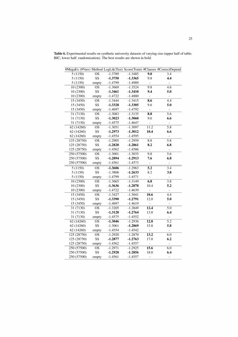
Table 6. Experimental results on synthetic university datasets of varying size (upper half of table:BIC; lower half: randomization). The best results are shown in bold.

#MegaEx (#Vars) Method LogLik(Test) Score(Train) #Clauses #CorrectDepend5 (1150) OS -1.3789 -1.3485 9.0 3.45 (1150) SS -1.3750 -1.3365 9.8 4.45 (1150) empty -1.4799 -1.4989 - -10 (2300) OS -1.3669 -1.3524 9.8 4.610 (2300) SS -1.3461 -1.3410 9.4 5.010 (2300) empty -1.4722 -1.4880 - -15 (3450) OS -1.3444 -1.3415 8.6 4.415 (3450) SS -1.3328 -1.3305 9.6 5.015 (3450) empty -1.4697 -1.4792 - -31 (7130) OS -1.3083 -1.3135 8.8 5.631 (7130) SS -1.3023 -1.3060 9.6 6.631 (7130) empty -1.4575 -1.4647 - -62 (14260) OS -1.3051 -1.3097 11.2 5.862 (14260) SS -1.2973 -1.3012 10.4 6.662 (14260) empty -1.4554 -1.4595 - -125 (28750) OS -1.2905 -1.2959 8.8 5.8125 (28750) SS -1.2828 -1.2861 8.2 6.8125 (28750) empty -1.4562 -1.4586 - -250 (57500) OS -1.3001 -1.3035 9.8 5.6250 (57500) SS -1.2894 -1.2913 7.6 6.8250 (57500) empty -1.4561 -1.4573 - -

5 (1150) OS -1.3606 -1.2963 5.2 3.45 (1150) SS -1.3806 -1.2633 8.2 3.85 (1150) empty -1.4799 -1.4571 - -10 (2300) OS -1.3665 -1.3149 6.8 3.810 (2300) SS -1.3636 -1.2878 10.4 5.210 (2300) empty -1.4722 -1.4639 - -15 (3450) OS -1.3427 -1.3041 10.6 4.415 (3450) SS -1.3390 -1.2791 12.0 5.015 (3450) empty -1.4697 -1.4619 - -31 (7130) OS -1.3205 -1.2849 12.4 5.031 (7130) SS -1.3128 -1.2764 13.0 6.431 (7130) empty -1.4575 -1.4552 - -62 (14260) OS -1.3046 -1.2936 12.8 5.262 (14260) SS -1.3061 -1.2869 15.8 5.862 (14260) empty -1.4554 -1.4542 - -125 (28750) OS -1.2920 -1.2870 13.2 6.0125 (28750) SS -1.2877 -1.2763 17.0 6.2125 (28750) empty -1.4562 -1.4557 - -250 (57500) OS -1.2971 -1.2925 15.6 6.0250 (57500) SS -1.2928 -1.2856 18.0 6.4250 (57500) empty -1.4561 -1.4557 - -

26

Table 7. Detailed timings for synthetic university datasets of varying size (upper half of table:BIC; lower half: randomization).

#MegaEx (#Vars) Method Ttotal Tinit Tfirst Trest I Tavg

5 (1150) OS 35s 7s 15s 13s 2.4 6s5 (1150) SS 137s 7s 60s 70s 5.8 12s10 (2300) OS 42s 7s 20s 15s 2.0 7s10 (2300) SS 134s 7s 69s 57s 4.2 13s15 (3450) OS 51s 8s 18s 24s 3.0 8s15 (3450) SS 164s 8s 73s 83s 5.8 14s31 (7130) OS 55s 10s 24s 20s 2.2 9s31 (7130) SS 168s 10s 85s 73s 4.6 16s62 (14260) OS 78s 13s 31s 34s 2.8 12s62 (14260) SS 262s 13s 101s 147s 6.2 24s125 (28750) OS 120s 18s 45s 57s 3.2 19s125 (28750) SS 407s 18s 161s 228s 4.4 56s250 (57500) OS 194s 33s 89s 71s 2.2 33s250 (57500) SS 586s 33s 246s 307s 4.8 66s

5 (1150) OS 31s 7s 17s 7s 1.2 6s5 (1150) SS 120s 7s 64s 49s 4.0 13s10 (2300) OS 42s 8s 20s 15s 2.0 8s10 (2300) SS 167s 8s 70s 89s 6.0 14s15 (3450) OS 56s 10s 25s 22s 2.6 8s15 (3450) SS 202s 10s 79s 11s4 6.8 17s31 (7130) OS 74s 11s 28s 35s 2.8 13s31 (7130) SS 256s 11s 92s 152s 6.8 21s62 (14260) OS 124s 19s 36s 68s 4.6 14s62 (14260) SS 415s 19s 124s 272s 8.2 33s125 (28750) OS 171s 31s 58s 82s 4.2 21s125 (28750) SS 692s 31s 192s 470s 10.2 46s250 (57500) OS 321s 56s 102s 164s 3.8 43s250 (57500) SS 1179s 56s 358s 765s 8.6 88s