REPORT - fudinfo.trafikverket.sefudinfo.trafikverket.se/fudinfoexternwebb/Publikationer... · In...

REPORT

Contact person Date Reference Page

Mikael Lindgren 2015-06-24 MTk4P06467-2 1 (31) Measurement Technology +46 10 516 57 13 [email protected]

Trafikverket Petter Hafdell Solna Strandväg 98 172 90 Sundbyberg

Final report - Traffic compensated luminance estimation

SP Technical Research Institute of Sweden

Postal address Office location Phone / Fax / E-mail This document may not be reproduced other than in full, except with the prior written approval of SP. SP

Box 857 SE-501 15 BORÅS Sweden

Västeråsen Brinellgatan 4 SE-504 62 BORÅS

+46 10 516 50 00 +46 33 13 55 02 [email protected]

Abstract Active control of street light sources based on sensor data is desired to meet requirements on traffic safety and environmental protection. In this report, we summarise the results of a research study focusing on some of the fundamental problems occurring when performing real-world sensor measurements for lighting control. In particular, we present results on the impact of traffic and the relationship between sensor angle and measured road surface luminance. Moreover, we present a comparison between different approaches to estimating the veiling luminance in tunnel lighting applications.

Contributing authors: Kenneth Jonsson, Cipherstone Technologies AB Mikael Lindgren, SP Technical Research Institute of Sweden Björn Löfving, University of Gothenburg Rene Nilsson, Cipherstone Technologies AB Jörgen Thaung, University of Gothenburg

REPORT

Date Reference Page

2015-06-24 MTk4P06467-2 2 (31)


1 Introduction International standards such as EN 13201 (CEN, 2004, 2003abc) require the amount of reflected light or road surface luminance to exceed a specified minimum level to allow the driver to identify objects of interest on the road with sufficient accuracy. At the same time, national transport administrations and local authorities face increasing demands on reducing the environmental impact by lowering energy consumption and consequently greenhouse gas emissions. Thus, in general, there is a desire to keep the luminance at the minimum required level. However, as the road surface characteristics change continuously over time due to ageing and varying weather conditions, the actual luminance may change dramatically over time and the use of active control to optimize light source output is needed to maintain the luminance at the desired level.

The active control of road light sources is a problem for which no cost-effective solution has been available until recently. Modern lighting control systems in combination with the new generation of light source technology such as light emitting diodes (LEDs) now allow continuous adjustments of street light output to meet the requirements on both traffic safety and environmental protection. To reflect the actual conditions, the control of light sources needs to be based on continuously updated sensor data from e.g. illuminance or luminance meters. The lighting control system may also integrate information from traffic sensors such as inductive loops, video analysis and radar systems. Moreover, wind meters, road surface friction meters and visibility sensors may be employed to provide data to a lighting control system.

In this report, we detail a research project aiming to study some of the fundamental problems occurring when measuring luminance in real-world traffic applications. Recent standards such as EN 13201 require the measurement of road surface luminance. However, in urban areas, the road surface is frequently covered with vehicles and the typical measurement will include light reflected from both the vehicle roof tops and from the road. As 25 percent of new cars worldwide have white colour this may result in a significant luminance error (PPG, 2013). In this report, we present results from field tests using a novel patent pending approach where light and traffic measurements are integrated to ensure that the measured luminance only includes contributions from the road surface. This is achieved by continuously tracking the vehicles using a prototype camera system employing advanced image analysis to block out image areas with vehicles from the luminance measurements.

Another problem of interest is the angle dependency in luminance estimation. Ideally, the road surface luminance should be measured at a position identical to the average driver position, i.e. in the middle of the lane and at approximately 1,5 meters above the road surface, as dictated in EN 13201. In practice, this may be accomplished when verifying a lighting installation by taking measurement from within a moving vehicle but not when continuously monitoring road surface luminance using a stationary sensor. In this report, we present the results of experiments aiming to investigate the relationships between sensor position, angle and surface characteristics. Measurements were taken from a selection of dry and wet road surface samples by varying the angle of the sensor in relation to the samples.

Finally, we also present results from a tunnel lighting application. The task was to calculate daytime lighting levels for the threshold zone of long tunnels using the “perceived contrast method” described in (CIE, 2004). For this application, the traffic compensated luminance camera was located at the stopping distance from the tunnel entrance and the system dynamically calculated the veiling luminance, Lseq, contribution to the tunnel entrance which is a key parameter for further calculation of the preferred luminance in the tunnel. By continuously monitoring the field of view for drivers approaching a tunnel, the lighting in the

REPORT

Date Reference Page

2015-06-24 MTk4P06467-2 3 (31)


threshold zone can be optimized for best quality of vision and an early warning system can be activated if the visibility drops because of increased disability glare in the field of view.

In the following section, we present the methods employed to calibrate the system and to analyse the traffic scene. Then, in the next section, we detail the measurement setup including the hardware configuration and the geometry of the installation. In the subsequent sections, we list the results obtained when studying specific problems such as the influence of traffic and the angle dependency. Finally, we discuss possible future research work and draw conclusions.

REPORT

Date Reference Page

2015-06-24 MTk4P06467-2 4 (31)


2 Methodology In this section, we detail the procedure for calibrating the prototype video photometer and the methods applied for real-time analysis of the traffic scene.

2.1 Camera calibration

The prototype video photometer is corrected for spectral, spatial and temporal response artefacts of the system. These artefacts originate from the different system sub-components and their settings. The spectral response of a number of samples of all sub-components of the system was measured over the visible range between 380 nm and 780 nm. Based on this information a suitable optical filter was selected resulting in an overall spectral response close to the CIE 1931 photopic luminosity function (CIE, 1932). The filter was placed in the optical path between the lens and the sensor.

The spatial artefacts of interest are primarily optical distortion and vignetting. The distortion of the system, which is a third order lens aberration, was measured with a dot chart (from Image Engineering GmbH, see Figure 1) under uniform incandescent lamp illumination. Vignetting of light that passes the system and gives rise to a relative signal degradation towards each corner of the image was measured by the use of an integrating sphere equipped with a light source suitable for the application.

Figure 1. Dot chart from Image Engineering, model TE 260.

The correction for vignetting is illustrated in Figure 2. The top row shows the result of correcting a single image of a white uniform surface (left is raw data colour coded, and right is the result after correction). The bottom row shows the result of correcting an average image (generated from 50 samples) of the same uniform surface (left is average raw data colour coded, and right is the result after correction). The benefits of averaging is clear from the figure – the signal-to-noise ratio is improved significantly after averaging.

REPORT

Date Reference Page

2015-06-24 MTk4P06467-2 5 (31)


Figure 2. Correction for vignetting: Single image before (top left) and after (top right) correction, average image before (bottom left) and after (bottom right) correction.

To capture the luminance information of the scene accurately the video photometer was finally calibrated against a luminance reference, using the same setup as for the vignetting measurements. The calibration of the system was done with the selected f-number, correct focus setting, suitable set of integration times, optimum gain and required frame rate. A large number of images were averaged to reduce the noise in the measurements before the data was fitted to a first order regression model.

For the tunnel measurements, the system was calibrated for four integration times with the same gain settings allowing the resulting images to be combined into a high dynamic range image. In the case of EN 13201, the system was calibrated for two different gain settings to make maximum use of the analogue to digital converter range and to increase the dynamic range of the system under the limitation of the maximum allowed integration time for traffic analysis.

2.2 Video analysis

The prototype system continuously analyses video frames at a rate of at least 40 frames per second. The relatively high frame rate is required to capture high dynamic range data (multiple exposure times) while keeping track of vehicles moving at high speed. The resulting data rate is high, meaning that we need to keep the complexity of operations low. The first step is to analyse the video frames corresponding to the different exposure times to determine which one provides the optimal non-saturated representation of the vehicles. The analysis is then restricted to the chosen frame. To further reduce the complexity, we restrict the subsequent operations to the region of interest for traffic analysis – the area of the chosen image occupied by road surface. Finally we apply a dynamic model to select the subset of pixels that belong to the road surface and reject the pixels that belong to potential vehicles on the road. The selected

REPORT

Date Reference Page

2015-06-24 MTk4P06467-2 6 (31)


pixels will then contribute to the luminance estimate while the rejected will not. This model is continuously updated to reflect low-frequency changes in time due to varying lighting conditions, without incorporating the high-frequency changes introduced by vehicles.

3 Luminance estimation In this section, we summarise the measurements performed using the prototype video photometer. We detail the prototype hardware, the two installation sites, and the measurements undertaken at these sites.

3.1 Prototype hardware

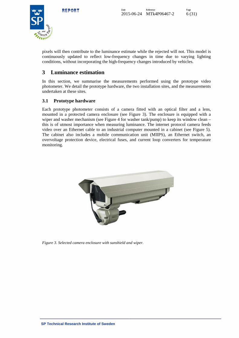
Each prototype photometer consists of a camera fitted with an optical filter and a lens, mounted in a protected camera enclosure (see Figure 3). The enclosure is equipped with a wiper and washer mechanism (see Figure 4 for washer tank/pump) to keep its window clean – this is of utmost importance when measuring luminance. The internet protocol camera feeds video over an Ethernet cable to an industrial computer mounted in a cabinet (see Figure 5). The cabinet also includes a mobile communication unit (MIIPS), an Ethernet switch, an overvoltage protection device, electrical fuses, and current loop converters for temperature monitoring.

Figure 3. Selected camera enclosure with sunshield and wiper.

REPORT

Date Reference Page

2015-06-24 MTk4P06467-2 7 (31)


Figure 4. Washer tank, pump and controller unit (two different versions used).

Figure 5. Cabinet with computer, communication unit (MIIPS) etc.

3.2 Installation sites

We have installed four prototypes at two different locations in the Gothenburg area in Sweden. At the EN 13201 site (see Figure 6) two cameras overview a stretch of an orbital four-lane motorway with a yearly average day traffic (ÅDT) of between 49 000 and 53 000 (2010). This is a busy route connecting the south and east part of the town with one of the main industrial areas in the west. The road is equipped with 123 W LED lighting (supplier Thorn Lighting, model “Victor LED”) with a 30 percent automatic power reduction during the 6 darkest hours of the day (as determined from a built-in sensor). At this particular site, the lights are mounted at a height of 10 m and the distance between the light poles is 48 m. The road has a lighting

REPORT

Date Reference Page

2015-06-24 MTk4P06467-2 8 (31)


class of ME3 (CEN, 2003) meaning that the average road surface luminance should not fall below 1,0 cd/m2 in dry road conditions.

Figure 6. Test site for measuring luminance according to EN 13201.

At the EN 13201 site, the cameras are mounted on a road portal overlooking an area between two street lights, as dictated in EN 13201. The distance between the portal and the nearest street light is approximately 44 m – note that this is less than the 60 m defined in EN 13201. We believe that this distance is representative for the distances that will be used in practice when monitoring road surface luminance in fixed installations. In a typical installation, we would mount the sensor on the light pole preceding the starting pole of the measurement area. By using existing infrastructure we can keep the installation costs low.

The first camera is mounted at a height of 7,4 m above the road surface and is centred horizontally on the left lane. The second camera is mounted at a height of 8,8 m and is centred on the right lane. Consequently, the horizontal distance between the two cameras is one lane width or 3,5 m.

Example scenes from the two prototype cameras at this site are shown in Figure 7 with EN 13201 measurement grids overlaid (blue colour). The green solid rectangles indicate the boundaries of the measurement areas – one for each lane. As can be seen in the pictures, measurement points are frequently covered by vehicles.

Figure 7. EN 13201 installation: Camera images with measurement points overlaid.

REPORT

Date Reference Page

2015-06-24 MTk4P06467-2 9 (31)


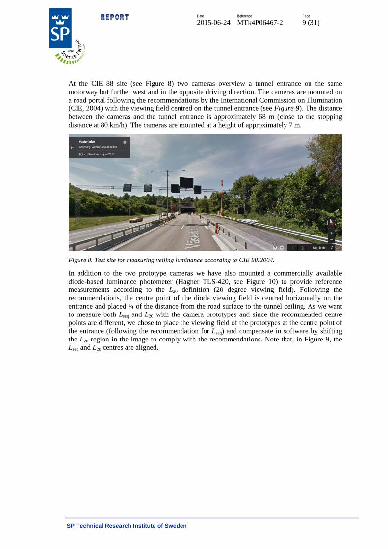
At the CIE 88 site (see Figure 8) two cameras overview a tunnel entrance on the same motorway but further west and in the opposite driving direction. The cameras are mounted on a road portal following the recommendations by the International Commission on Illumination (CIE, 2004) with the viewing field centred on the tunnel entrance (see Figure 9). The distance between the cameras and the tunnel entrance is approximately 68 m (close to the stopping distance at 80 km/h). The cameras are mounted at a height of approximately 7 m.

Figure 8. Test site for measuring veiling luminance according to CIE 88:2004.

In addition to the two prototype cameras we have also mounted a commercially available diode-based luminance photometer (Hagner TLS-420, see Figure 10) to provide reference measurements according to the L20 definition (20 degree viewing field). Following the recommendations, the centre point of the diode viewing field is centred horizontally on the entrance and placed ¼ of the distance from the road surface to the tunnel ceiling. As we want to measure both Lseq and L20 with the camera prototypes and since the recommended centre points are different, we chose to place the viewing field of the prototypes at the centre point of the entrance (following the recommendation for Lseq) and compensate in software by shifting the L20 region in the image to comply with the recommendations. Note that, in Figure 9, the Lseq and L20 centres are aligned.

REPORT

Date Reference Page

2015-06-24 MTk4P06467-2 10 (31)


Figure 9. CIE 88 installation: Prototypes (left) and Lseq and L20 diagrams (right).

Figure 10. Commercially available diode-based luminance photometer: Hagner TLS-420.

3.3 Centring the field of view

As noted above, the centring of the viewing field is an important part of the installation procedure. To investigate how sensitive the luminance measurements are to the viewing field we selected data from a clear day and varied the vertical and horizontal position of the L20 measurement area in the luminance image. Note that this constitutes a translation of the viewing field and is not exactly equivalent to a change of viewing field resulting from a camera rotation. In Figure 11, we show the relative luminance error as a function of the vertical or horizontal displacement, and the corresponding heat map (with relative luminance error colour coded, black is 0,0 and white is 1,0, colour sequence is black-red-orange-yellow-white, maximum error in Figure 11 is 0,63 or 63 percent). As expected, vertical displacements have a strong impact on the luminance. For this particular sunny day in April, a vertical shift of 12 pixels (or 2 percent of the number of image lines) corresponding to the distance between the Lseq and L20 centre points results in a relative luminance shift of 7,6 percent. Over a longer time period (see Table 1), we have estimated the average luminance shift to 5,4 percent.

REPORT

Date Reference Page

2015-06-24 MTk4P06467-2 11 (31)


Figure 11. Relationship between relative luminance error and displacement.

3.4 Long-term measurements

In Table 1, we show summary statistics for the L20 and Lseq measurements for different viewing field centre points and with/without traffic compensation (TC). We show the mean and maximum luminance values as well as the deviation (Δ) with respect to the reference configuration (top row) in percentages.

Table 1. Summary statistics: Period 2015-04-15 to 2015-05-11 (27 days).

Measurement

Centre TC Mean (cd/m2)

Δ (%)

Max (cd/m2)

Δ (%)

L20 ½ Yes 608 0,0 3785

0,0

L20 ½ No 595 2,1 4145 9,5

L20 ¼ Yes 641 5,4 4127 9,0

L20 ¼ No 627 3,1 4525 19,6

Lseq ½ Yes 30 N/A 186 N/A

3.5 Traffic compensation

The objective of the study reported in this section was to investigate the impact of traffic on the luminance estimation. The results are compiled from the EN 13201 site where the field of view is dominated by road surface and the impact of traffic is likely to be the highest. The measurements were carried out in April and May and, unfortunately, during this period of the year, peak traffic times do not coincide with twilight or nocturnal conditions (the conditions of interest in dimming of street lights). Therefore the luminance values reported below are from daytime scenes only.

In Figure 12 and Figure 13, we show the average luminance computed over the EN 13201 measurement grid as a function of time for parts of two days. We show the average luminance

REPORT

Date Reference Page

2015-06-24 MTk4P06467-2 12 (31)


with (blue line) and without (light blue line) traffic compensation. Moreover, we show the result of applying a one-dimensional infinite impulse response (IIR) filter to the uncompensated signal (green line). The IIR filter is included for comparison and represents a best-effort approach to smooth the one-dimensional raw signal (in a real-world scenario the raw signal would not be used directly to control the lighting). The relative error between the filtered uncompensated and compensated signals is also shown (light red line).

In Figure 12, we can see several periods where the uncompensated and filtered uncompensated signals both deviate significantly from the compensated signal. For example, the 16-minute period between 14:45 and 15:01 where the relative error is around 8 - 10 percent. The average traffic flow at 14:55 was 3555 vehicles per hour (as measured by inductive loops) which is the peak flow between 14:30 and 15:30.

Figure 12. Traffic compensation vs no compensation: Tuesday 2015-04-28.

In Figure 13, we can see a distinct deviation around 08:40 in the morning where the relative error is 73 percent. This deviation coincides with the peak traffic flow between 08:15 and noon which is 3864 vehicles per hour.

REPORT

Date Reference Page

2015-06-24 MTk4P06467-2 13 (31)


Figure 13. Traffic compensation vs no compensation: Monday 2015-05-11.

As noted above, there is a correlation between traffic density and uncompensated luminance. But there are also other factors affecting the luminance such as the colour and size distribution of the vehicles, and the shadows vehicles may cast on the road. For example, a large white (or black) lorry may have a significant impact on the luminance but only a minor effect on the density.

In Figure 14, Figure 15 and Figure 16, we illustrate the effect of traffic compensation by overlaying the EN 13201 measurement points on camera images. The measurement points are colour coded using a heat map (matlab ‘jet’) with colour sequence blue-yellow-orange-red corresponding to low-to-high luminance values. In Figure 14, we show a reference scene without traffic. In Figure 15, we show a scene with a lorry passing and without traffic compensation activated. Finally, in Figure 16, we show the same scene as in Figure 15 but with traffic compensation activated. As can be seen in the last two figures, the two columns of measurement points to the right in the images are clearly affected by the passing lorry. Note that the colour coding is applied with transparency, meaning that the heat map colour for a measurement point is mixed with the local image colour. In Figure 15 and 16, the effect of traffic compensation is most clearly visible in the dark regions at the back of the lorry (lower right corner of images).

REPORT

Date Reference Page

2015-06-24 MTk4P06467-2 14 (31)


Figure 14. EN 13201 measurement grid overlaid on camera image, reference scene.

Figure 15. EN 13201 measurement grid, without traffic compensation.

REPORT

Date Reference Page

2015-06-24 MTk4P06467-2 15 (31)


Figure 16. EN 13201 measurement grid, with traffic compensation.

3.6 Angle dependencies

The continuous monitoring of road surface luminance requires a sensor position which deviates substantially from the requirements in EN 13201. There are well developed methods for determining the luminance coefficient of tarmac (CIE, 1982, 1999), but little data is available for other (higher) observation angles than the prescribed 1° (Ekrias, Ylinen). For the purpose of the proposed method of luminance measurement, it is necessary to mount the sensor at observation angles in the range 4° – 10°. The resulting measurement of luminance will therefore differ from the road surface luminance experienced by the vehicle driver by an unknown amount. In addition, the difference may vary due to external factors, e.g. tarmac type, age and/or weather conditions. In order to investigate the dependency of luminance on the observation angle, measurements have been performed on two samples of used tarmac.

The setup for road lighting design uses the designations given in Figure 17.

REPORT

Date Reference Page

2015-06-24 MTk4P06467-2 16 (31)


Figure 17. Designation of angles used in description of road surface luminance coefficient, from CIE 132.

In the investigation described here, we have used an angle β = 0°, an illumination angle γ = 67,4°, and the observation angle α was varied from 1° up to ~30°. The choice of β and γ angles corresponds to the conditions of the field test site. In addition, a LED light source with ~4000 K correlated colour temperature was used and the luminous intensity of the light source was adapted by choosing a distance (P – A) so the illuminance on the road surface was in the same range as our field test site. Measurements were performed in the optics laboratory of SP in Borås, Sweden, under indoor conditions, see Figure 18.

Figure 18. Measurement setup for measuring tarmac reflectance angle dependency.

The road surface luminance was measured using a spot luminance meter (Photo Research PR-735). The acceptance angle of the meter was varied from 0,125° (for the lowest angle range) to 0,5°. The distance from the tarmac sample was ~4,0 m. In the investigation, two samples of used asphalt concrete of the size 0,4 × 0,6 m were utilized, placed horizontally. Measurements were performed on both dry and wet surfaces. The two samples differed in terms of the small and large aggregates, both taken from roads in the SP area.

LED lamp4000 K

Tarmac sampleObservation angle

Illuminationangle

Spectroradiometer

REPORT

Date Reference Page

2015-06-24 MTk4P06467-2 17 (31)


Results from measurement of luminance on dry surfaces are shown in Figure 19.

Figure 19. Results from measurements on dry road surface samples.

The results show that the perceived luminance decreases with increasing observation angle. However, the luminance shows large variation with sample (aggregate size), particularly in the lowest angle range. Also, in the range of interest for our application (4° - 10°) the results differ substantially.

Results from measurement of luminance on wet surfaces are shown in Figure 20.

Figure 20. Results from measurements on wet road surface samples.

The results show a substantially higher level for the perceived luminance and also a different dependence on the observation angle. Clearly, a wet surface must be handled differently than a dry surface.

The measurements show quite different results and stronger dependencies than reported elsewhere (Guo, 2007). It suggests that further investigation is necessary and perhaps that

0,0

0,5

1,0

1,5

2,0

2,5

0 5 10 15 20 25 30 35

Lum

inan

ce (c

d/m

2 )

Observation angle (deg)

Dry (small aggregate)

0

1

2

3

4

5

6

0 5 10 15 20 25 30 35

Lum

inan

ce (c

d/m

2 )Observation angle (deg)

Dry (large aggregate)

0

5

10

15

20

25

30

0 5 10 15 20 25 30 35

Lum

inan

ce (c

d/m

2 )


Wet (small aggregate)

0

20

40

60

80

100

120

140

160

0 5 10 15 20 25 30 35

Lum

inan

ce (c

d/m

2)


Wet (large aggregate)

Specularreflection

REPORT

Date Reference Page

2015-06-24 MTk4P06467-2 18 (31)


individual adaptation to the road surface conditions at the luminance measurement site is needed.

3.7 Veiling luminance estimation

3.7.1 Introduction to veiling luminance and disability glare

Veiling luminance arise in the human eye due to light scattering in mainly the lens, cornea and retina. The veiling luminance will be superimposed on the retinal image and will reduce the contrast levels. This will degrade the visual quality as low contrast objects might become undetectable. When vision is degraded in this way it is called “veiling glare”, which is defined in the CIE e-ILV Termlist:

Veiling glare: light, reflected from an imaging medium, that has not been modulated by the means used to produce the image.

NOTE 1 veiling glare lightens and reduces the contrast of the darker parts of an image.

NOTE 2 the veiling glare is sometimes referred to as "ambient flare”.

Another CIE term that is a little more general is:

Disability glare: glare that impairs the vision of objects without necessarily causing discomfort.

The most general term “glare” also includes situations where discomfort is experienced, but can also mean veiling and disability glare. According to CIE, the definition is:

glare: condition of vision in which there is discomfort or a reduction in the ability to see details or objects, caused by an unsuitable distribution or range of luminance, or by extreme contrasts.

There is always some degree of veiling luminance in the human eye, but for an observer with normal eyes, the observer might not be aware of any veiling glare or disability glare until the visual ability is put to the test. A particularly difficult visual task is to detect objects in a dark region of the field of view when there are much brighter regions present at the same time. Bright areas tend to “smear out” and mask dark areas of the image because the proportion of scattered light is high compared to the amount of light forming an image in the dark areas. Sometimes it is easy to determine if the veiling luminance from a specific light source or bright area causes disability glare or not, by temporarily obscuring it with the hand. If the contrast in the view increases when the light source is obscured, it causes disability glare. When the light source is no longer present in the field of view, the veiling luminance immediately also disappears and the image quality improves.

3.7.2 Mathematical description of veiling luminance

In (CIE. 1999b) mathematical descriptions of veiling luminance, Leq, are presented. Leq for a normal observer that doesn’t suffer from any eye disease, depends mainly on the angle to the glare source, age and eye colour. The scattered light increases with age and is commonly referred to as a consequence of normal ageing. The eye colour affects the scattered light in the eye because a dark iris more efficiently blocks light from entering the eye because of higher absorption than a blue pigmented iris.

The most complete formula for calculating Leq, often referred to as “the best mathematical description of the foveal visual point spread function at the present state of knowledge”, is:

REPORT

Date Reference Page

2015-06-24 MTk4P06467-2 19 (31)


𝐿eq 𝐸gl⁄ = �1 − 0,08 �𝐴

70�4� �

9,2 ∙ 106

[1 + (Θ 0,0046⁄ )2]1,5 +1,5 ∙ 105

[1 + (Θ 0,045⁄ )2]1,5�

+ �1 + 1,6 �𝐴

70�4� ��

4001 + (Θ 0,1⁄ )2 + 3 ∙ 10−8 ∙ Θ2�

+ 𝑝 �1300

[1 + (Θ 0,1⁄ )2]1,5 +0,8

[1 + (Θ 0,1⁄ )2]0,5��+ 2,5 ∙ 10−3𝑝 [𝑠𝑠−1]

… eq. (1)

where Leq = equivalent veiling luminance, in cd/m2; Egl = glare illuminance at the eye, in lux; Θ = glare angle in degrees, 0° < Θ < 100°; A = age; p = pigmentation factor (p = 0 for very dark eyes, p = 0,5 for brown eyes, and p = 1,0 for blue-green Caucasians), cf. (CIE. 1999b).

In this equation, the glare source is expressed as an illuminance in “lux”, Egl. If instead the luminance of the glare source, Lgl, is known from a luminance measurement for example, Lgl has to be multiplied by its solid angle viewed from the observer. To calculate the veiling luminance contribution Leq,i from a luminance image “pixel” with luminance Li, it has to be multiplied with the solid angle of that pixel from the position of the observer to obtain Egl,i:

𝐸gl,i = 𝐿i ∙ Ωi …eq. (2)

where Ωi is the solid angle of the glare source (pixel) from the position of the observer (camera).

Eq. (1) can be approximated to a large extent. A simple approximation called “Age Adapted Stiles-Holaday Glare Equation” (AASH) cf. (CIE. 1999b), still constitutes a good estimate for the veiling luminance in the range 3° < Θ < 30° and reads:

𝐿eq 𝐸gl⁄ = �1 + � 𝐴70�

4� ∙ 10

Θ2 for 3° < Θ < 30° …eq. (3)

Figure 21 shows the complete glare function calculated for the ages 35 and 80 years (with p = 1) and the AASH approximation plotted together. AASH is a good approximation in the range 2° < Θ < 30°.

REPORT

Date Reference Page

2015-06-24 MTk4P06467-2 20 (31)


Figure 21. The complete veiling glare function and the Age adapted Stiles-Holaday approximation plotted together.

3.7.3 Application of the veiling glare function

In the CIE. 2004 document it is recommended to control the lighting in the threshold zone of tunnels with an estimate to the veiling luminance, Lseq, as an input parameter.

Lseq, is calculated based on the relation for the veiling luminance:

Leq Egl⁄ = �1 + � A70�4� ∙ 10

Θ2 for 3° < Θ < 30° …eq. (3)

The veiling luminance is calculated in one position in the centre of the tunnel opening viewed from the “stopping distance” in front of the tunnel.

Lseq is calculated by summing luminance contributions from 108 sections in the angular range of 1° < Θ < 28°. The size of the sections is chosen so that the average luminance occurring in them, Li, contributes equally to the veiling luminance. That means the area of the sections is proportional to Θ-2.

𝐿seq = 5,1 ∙ 10−4 �𝐿I,e

𝑁

i=1

…eq. (4)

where Li,e is the average luminance of section i (measured in front of the eye) and N is the total number of sections. See Figure 9 right where the sections are drawn.

To confirm the correctness of the Lseq implementation, and possible effects due to the calculation based on the limited number of sections, we have compared Lseq with calculations of the veiling luminance, Leq, based on eq. (1) that uses all image points in a luminance image L. Leq was calculated in all image points and added to L to obtain a visualization of the contrast reduction. Such an image is shown in the right half of Figure 22 (left).

Five luminance images representing the highest Lseq, L20, and maximum ratios L20/Lseq, Lseq/L20, and Lseq/L2 respectively, were extracted from the measurement period in order to investigate Lseq and veiling luminance estimations. (L2 and L20 are the average luminance computed over a

REPORT

Date Reference Page

2015-06-24 MTk4P06467-2 21 (31)


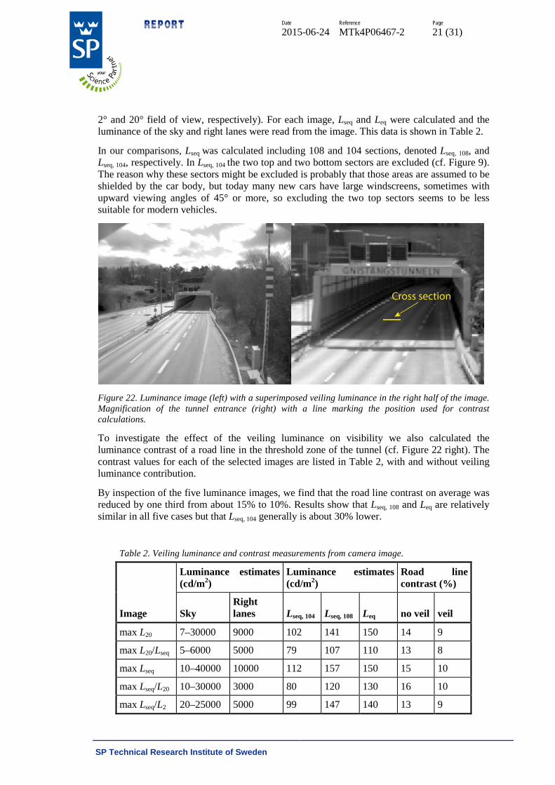
2° and 20° field of view, respectively). For each image, Lseq and Leq were calculated and the luminance of the sky and right lanes were read from the image. This data is shown in Table 2.

In our comparisons, Lseq was calculated including 108 and 104 sections, denoted Lseq, 108, and Lseq, 104, respectively. In Lseq, 104 the two top and two bottom sectors are excluded (cf. Figure 9). The reason why these sectors might be excluded is probably that those areas are assumed to be shielded by the car body, but today many new cars have large windscreens, sometimes with upward viewing angles of 45° or more, so excluding the two top sectors seems to be less suitable for modern vehicles.

Figure 22. Luminance image (left) with a superimposed veiling luminance in the right half of the image. Magnification of the tunnel entrance (right) with a line marking the position used for contrast calculations.

To investigate the effect of the veiling luminance on visibility we also calculated the luminance contrast of a road line in the threshold zone of the tunnel (cf. Figure 22 right). The contrast values for each of the selected images are listed in Table 2, with and without veiling luminance contribution.

By inspection of the five luminance images, we find that the road line contrast on average was reduced by one third from about 15% to 10%. Results show that Lseq, 108 and Leq are relatively similar in all five cases but that Lseq, 104 generally is about 30% lower.

Table 2. Veiling luminance and contrast measurements from camera image.

Image

Luminance estimates (cd/m2)

Luminance estimates (cd/m2)

Road line contrast (%)

Sky Right lanes Lseq, 104 Lseq, 108 Leq no veil veil

max L20 7–30000 9000 102 141 150 14 9

max L20/Lseq 5–6000 5000 79 107 110 13 8

max Lseq 10–40000 10000 112 157 150 15 10

max Lseq/L20 10–30000 3000 80 120 130 16 10

max Lseq/L2 20–25000 5000 99 147 140 13 9

REPORT

Date Reference Page

2015-06-24 MTk4P06467-2 22 (31)


3.7.4 Comparison between Lseq and L20

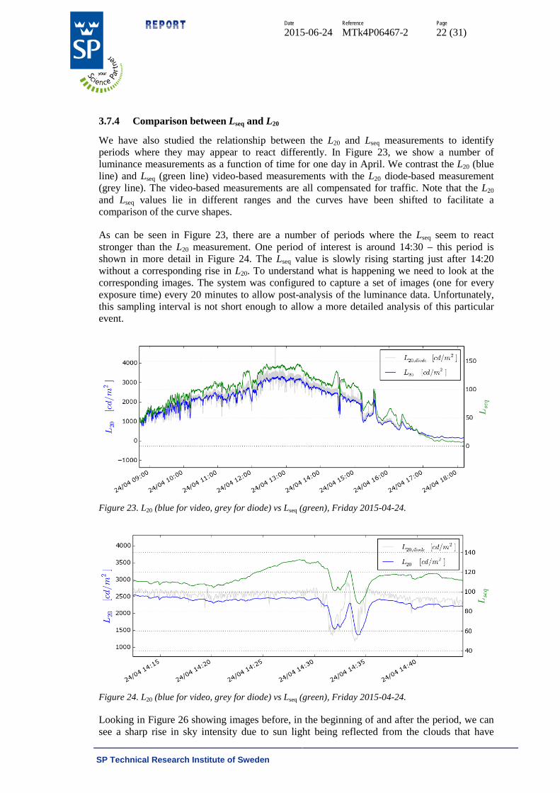
We have also studied the relationship between the L20 and Lseq measurements to identify periods where they may appear to react differently. In Figure 23, we show a number of luminance measurements as a function of time for one day in April. We contrast the L20 (blue line) and Lseq (green line) video-based measurements with the L20 diode-based measurement (grey line). The video-based measurements are all compensated for traffic. Note that the L20 and Lseq values lie in different ranges and the curves have been shifted to facilitate a comparison of the curve shapes.

As can be seen in Figure 23, there are a number of periods where the Lseq seem to react stronger than the L20 measurement. One period of interest is around 14:30 – this period is shown in more detail in Figure 24. The Lseq value is slowly rising starting just after 14:20 without a corresponding rise in L20. To understand what is happening we need to look at the corresponding images. The system was configured to capture a set of images (one for every exposure time) every 20 minutes to allow post-analysis of the luminance data. Unfortunately, this sampling interval is not short enough to allow a more detailed analysis of this particular event.

Figure 23. L20 (blue for video, grey for diode) vs Lseq (green), Friday 2015-04-24.

Figure 24. L20 (blue for video, grey for diode) vs Lseq (green), Friday 2015-04-24.

Looking in Figure 26 showing images before, in the beginning of and after the period, we can see a sharp rise in sky intensity due to sun light being reflected from the clouds that have

REPORT

Date Reference Page

2015-06-24 MTk4P06467-2 23 (31)


drifted in. This increase in light levels is not reflected in the L20 measurements as the L20 region only includes a small part of the sky area. The benefits of Lseq are clear in the case when the sun is present within the field of view. However, this period is an interesting example of another scenario when the Lseq measurement is superior to the L20 – when light is reflected into the scene from clouds.

3.7.5 Contributions from individual Lseq-sections

To investigate the contribution from individual Lseq-sections in a specific traffic environment, each section was visually identified using the luminance camera image with superimposed sectors. Eight sections representing contributions from the sky were identified and marked with blue patches (cf. Figure 25). Sections corresponding to road surface were marked with a grey patch (28 sections), and sections corresponding to vegetation or other areas (e.g. dark surfaces in the tunnel) were marked with green patches. By individually summing contributions in the three categories (Lseq for blue, green and grey areas) a comparison between the three categories could be made. Nine images during a 25-minute period were examined.

When calculating Lseq, 104 (top two and bottom two sectors excluded) the road surface was the dominant contributor in seven of the nine calculations. An interesting finding was that the sky category never was the dominant source to Lseq, 104.

When calculating Lseq, 108 (all sections included) the sky was the dominant contributor to Lseq in six of the nine calculations. Despite the two extra sections detecting road surface contribution, the top two sections detecting the sky were even stronger giving the sky category the largest impact on the Lseq, 108 calculation. Since many new cars have large windscreens it may seem strange that these Lseq - sections are excluded as discussed in Section 3.7.3.

Figure 25. Luminance camera image with superposition of all 108 Lseq-sections. Each individual section is marked with a patch that indicates if the major contribution comes from sky (blue), road (grey) or vegetation/other areas (green). In calculation on Lseq,104 the top two and bottom two sections are excluded (light coloured patches with dotted border lines).

REPORT

Date Reference Page

2015-06-24 MTk4P06467-2 24 (31)


3.7.6 Error estimation in threshold zone luminance calculations

In CIE. 2004 it is recommended to use Lseq as a parameter for calculating the threshold zone luminance, Lth, in a tunnel. The formula for calculating Lth is derived from a visual situation where the contrast, Cm, of an obstacle on the road in the tunnel threshold zone, should be at least 28 %. Cm is referred to as “minimum perceived contrast” and is measured at the stopping distance.

The formula for calculating Lth can be found in CIE. 2004 and is not repeated here. We have calculated how an underestimation of Lseq might influence Cm. Two examples are given in Table 3 where we assume that Lseq is underestimated by 30 %. If Lth was calculated based on a too low Lseq the consequence would be that Cm would drop because of too little illumination.

Table 3. Example of error in minimum perceived contrast, Cm, because of an underestimation of the value of Lseq by 30 %.

Lseq (cd/m2)

Lseq − 30% (cd/m2)

Cm

Example 1 100 70 26 %

Example 2 200 140 25 %

We conclude that an underestimation of Lseq by 30 % gives a reduction in Cm of about 3 percentage points (28 % – 25 %) at these luminance levels. This impact has to be considered when deciding how the veiling luminance should be determined, so an adequate measure is used.

REPORT

Date Reference Page

2015-06-24 MTk4P06467-2 25 (31)


Figure 26. Before deviation period (14:03), start of period (14:24), and after period (14:45).

REPORT

Date Reference Page

2015-06-24 MTk4P06467-2 26 (31)


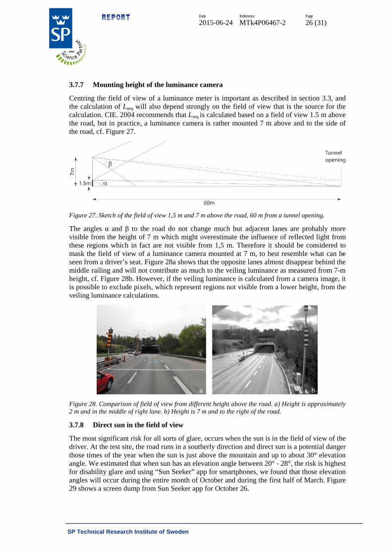
3.7.7 Mounting height of the luminance camera

Centring the field of view of a luminance meter is important as described in section 3.3, and the calculation of Lseq will also depend strongly on the field of view that is the source for the calculation. CIE. 2004 recommends that Lseq is calculated based on a field of view 1.5 m above the road, but in practice, a luminance camera is rather mounted 7 m above and to the side of the road, cf. Figure 27.

Figure 27. Sketch of the field of view 1,5 m and 7 m above the road, 60 m from a tunnel opening.

The angles α and β to the road do not change much but adjacent lanes are probably more visible from the height of 7 m which might overestimate the influence of reflected light from these regions which in fact are not visible from 1,5 m. Therefore it should be considered to mask the field of view of a luminance camera mounted at 7 m, to best resemble what can be seen from a driver’s seat. Figure 28a shows that the opposite lanes almost disappear behind the middle railing and will not contribute as much to the veiling luminance as measured from 7-m height, cf. Figure 28b. However, if the veiling luminance is calculated from a camera image, it is possible to exclude pixels, which represent regions not visible from a lower height, from the veiling luminance calculations.

Figure 28. Comparison of field of view from different height above the road. a) Height is approximately 2 m and in the middle of right lane. b) Height is 7 m and to the right of the road.

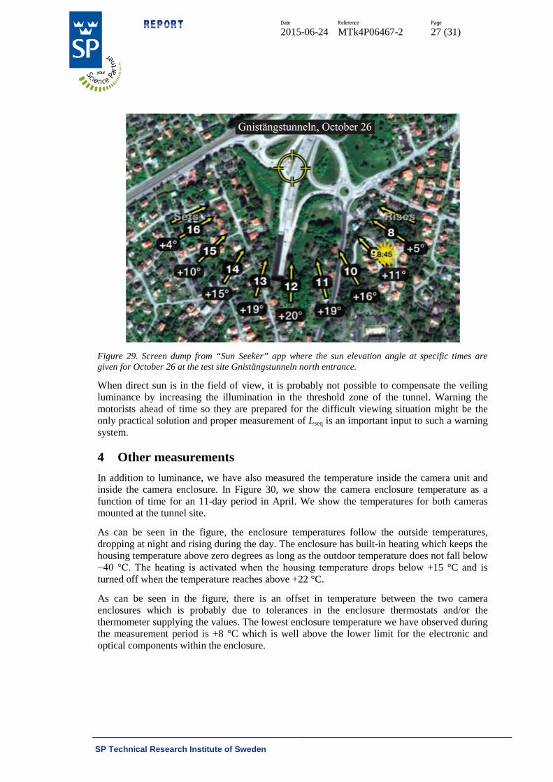
3.7.8 Direct sun in the field of view

The most significant risk for all sorts of glare, occurs when the sun is in the field of view of the driver. At the test site, the road runs in a southerly direction and direct sun is a potential danger those times of the year when the sun is just above the mountain and up to about 30° elevation angle. We estimated that when sun has an elevation angle between 20° - 28°, the risk is highest for disability glare and using “Sun Seeker” app for smartphones, we found that those elevation angles will occur during the entire month of October and during the first half of March. Figure 29 shows a screen dump from Sun Seeker app for October 26.

REPORT

Date Reference Page

2015-06-24 MTk4P06467-2 27 (31)


Figure 29. Screen dump from “Sun Seeker” app where the sun elevation angle at specific times are given for October 26 at the test site Gnistängstunneln north entrance.

When direct sun is in the field of view, it is probably not possible to compensate the veiling luminance by increasing the illumination in the threshold zone of the tunnel. Warning the motorists ahead of time so they are prepared for the difficult viewing situation might be the only practical solution and proper measurement of Lseq is an important input to such a warning system.

4 Other measurements In addition to luminance, we have also measured the temperature inside the camera unit and inside the camera enclosure. In Figure 30, we show the camera enclosure temperature as a function of time for an 11-day period in April. We show the temperatures for both cameras mounted at the tunnel site.

As can be seen in the figure, the enclosure temperatures follow the outside temperatures, dropping at night and rising during the day. The enclosure has built-in heating which keeps the housing temperature above zero degrees as long as the outdoor temperature does not fall below −40 °C. The heating is activated when the housing temperature drops below +15 °C and is turned off when the temperature reaches above +22 °C.

As can be seen in the figure, there is an offset in temperature between the two camera enclosures which is probably due to tolerances in the enclosure thermostats and/or the thermometer supplying the values. The lowest enclosure temperature we have observed during the measurement period is +8 °C which is well above the lower limit for the electronic and optical components within the enclosure.

REPORT

Date Reference Page

2015-06-24 MTk4P06467-2 28 (31)


Figure 30. Camera enclosure temperature over time (degrees Celsius).

REPORT

Date Reference Page

2015-06-24 MTk4P06467-2 29 (31)


5 Future work The prototype installations in Gothenburg will remain in operation until the end of the year. This means that there will be opportunities to study some of the above problems in more detail and under a larger set of conditions. In particular, we will be able to study the impact of traffic compensation during the late autumn when peak traffic density coincides with twilight and nocturnal conditions (when light dimming is applicable). Also, we will capture conditions in the autumn when the sun is at lower elevation angles and appears within the field of view, causing disability glare.

We have identified a number of areas where further research may be motivated:

• Angle dependence: The results obtained so far indicate a need for separate treatment of dry and wet road surfaces. However, it is not clear how this should be implemented and whether adaptations to the actual measurement sites may be required. Moreover, the preliminary results are based on a small sample count and the study needs to be extended to confirm the results on a larger sample set.

• Traffic compensation: As noted above, the measurement period does not include conditions when peak traffic coincides with twilight/nocturnal conditions. The conditions of interest will occur during the autumn and the analysis should then be repeated to determine the impact of traffic on luminance estimation.

• Field of view for veiling luminance camera: The calculated veiling luminance depends strongly on the field of view of the camera and should resemble the real situation for a driver, as closely as possible. Studying how to compensate the difference in field of view for a driver and for a camera would be valuable for correct calculation of the veiling luminance.

• Tunnel exit zones: In existing installations, the veiling luminance is monitored at the entrance of tunnels only. However, the lighting is dynamically adjusted in both the entrance and exit zones. A question that was raised during the project is if we need separate monitoring of veiling luminance in the exit zones of tunnels? And if so how do we measure veiling luminance from inside the tunnel?

• Sensor density and complexity: The prototype platform for EN 13201 measurements is suitable for low density installations (large number of lights per sensor). If we require higher density to accurately capture local variations in luminance levels, then another hardware solution may be required. A fundamental question to answer is what the acceptable luminance error is. Given a maximum luminance error we can determine suitable hardware (camera, optics etc). Then, given the hardware cost, we can decide on a density allowing the investment to be re-gained in terms of energy savings over a three or five year period.

REPORT

Date Reference Page

2015-06-24 MTk4P06467-2 30 (31)


6 Concluding remarks In this report, we summarised the results of a research study focusing on some of the fundamental problems occurring when performing real-world sensor measurements for lighting control. Our results indicate that traffic may have a significant impact on the road surface luminance estimates. Luminance errors in the order of 10 percent are common and may, in extreme cases, reach above 70 percent. We also studied the relationship between sensor angle and measured luminance. Further investigations are needed but the preliminary data indicate that dry and wet road surfaces may require separate treatment.

Our results regarding the veiling luminance indicate that it should be computed from all 108 sections as defined in CIE 88. By reducing the number of sections to the recommended 104, one may introduce an error in the luminance estimate which according to our measurements may reach 30 percent. Moreover, the results indicate a need for Lseq (as opposed to L20) even in scenarios when the sun is not present in the field of view. Sun light may be reflected from clouds causing a strong contribution from the upper sky sections in the Lseq diagram.

7 Acknowledgements This research study was funded by the National Transport Administration of Sweden to whom we are grateful for all support. Also, we would like to acknowledge the work carried out by engineers at SP Technical Research Institute of Sweden (Stefan Källberg) and Cipherstone Technologies AB (David Samuelsson, David Tingdahl and Gauthier Östervall). Their effort was invaluable in building/installing the prototypes and performing measurements.

REPORT

Date Reference Page

2015-06-24 MTk4P06467-2 31 (31)


8 References CEN. 2004. CEN/TR 13201-1:2004: E. Road lighting – Part 1: Selection of lighting classes. Brussels: CEN.

CEN. 2003a. EN 13201-2:2003 E. Road lighting – Part 2: Performance requirements. Brussels: CEN.

CEN. 2003b. EN 13201-3:2003 E. Road lighting – Part 3: Calculation of performance. Brussels: CEN.

CEN. 2003c. EN 13201-4:2003 E. Road lighting – Part 4: Methods of measuring lighting performance. Brussels: CEN.

CIE. 1932. Commission internationale de l’Eclairage proceedings, 1931. Cambridge: Cambridge University Press.

CIE. 1982. CIE 30-2:1982. Calculation and measurement of luminance and illuminance in road lighting. Computer program for luminance, illuminance and glare. Vienna: CIE.

CIE. 1999a. CIE 132:1999. Design Methods for Lighting of Roads. Vienna: CIE.

CIE. 1999b. CIE 135/1-1999. Report on disability glare. ISBN 3 900 734 97 6. Vienna: CIE.

CIE. 2004. CIE 88:2004. Guide for the lighting of road tunnels and underpasses. Vienna: CIE.

EKRIAS, A. 2010. Development and enhancement of road lighting principles. Report 56. Espoo: Aalto University.

GUO, L, ELOHOLMA, M, and HALONEN, L. 2007. Luminance monitoring and optimization of luminance metering in intelligent road lighting control systems. Ingineria Iluminatului, 9, 24 - 40.

JÄGERBRAND, A, CARLSON, A. 2011. Potential för en energieffektivare väg- och gatubelysning. VTI rapport 722. Stockholm: VTI.

PPG. 2013. “PPG data shows white continues to be most popular global car color”. Troy: PPG.

YLINEN, A, PUOLAKKA, M, and HALONEN, L. 2010. Road surface reflection properties and applicability of the R-tables for today’s pavement materials in Finland. Light & Engineering 18, 78-90.

SP Technical Research Institute of Sweden Measurement Technology - Communication Performed by

__Signature_1 __Signature_2

Mikael Lindgren

REPORT - fudinfo.trafikverket.sefudinfo.trafikverket.se/fudinfoexternwebb/Publikationer... · In...

Documents

Transcript of REPORT - fudinfo.trafikverket.sefudinfo.trafikverket.se/fudinfoexternwebb/Publikationer... · In...