REPORT DOCUMENTATION PAGE Form App ro ved … · REPORT DOCUMENTATION PAGE Form App ro ved OMB N o....

REPORT DOCUMENTATION PAGE Form Appro ved

OMB No. 0704-0 188

The public reponing burden for this collec tion ol informatiOn •s estimated to average 1 hour per response. including the ti~e for rev•ewing i':sHuction!., searching existing _data sou.rces .

gtnhenng and maimainmg the data needed, and completing and reviewing the collectron of in f~rmation. Send comment~ regar~mg th•s burden est•m a.te or ar1y other aspect o f th ts collect ton of

In formation, Including suggestions for reducing the burden, 10 Depanment of Defense. Washtngton Headquarters se.rvtces, !?•rectorate for lnfo_r':"a!IOO Op lf3tlons and Repor ts (07_04·0 188).

12 15 Jefferson Dav•s Highway. Su• te 1204, Arlington. VA 22202-4302. Respondents should be aware thaT noTw•Thstandrng any other provrsron of law, no person shall be subJeCT to any

penalty for failing to comply w11h a collectron of information if it does not display a currently valid OMS control number.

PLEA SE DO NOT RETURN YOUR FORM TO THE ABOVE ADDRESS.

1. REPORT DATE IDD-MM-YYYYJ Jz REPORT TYPE 3 . DATES COVERED !From - To)

11-05-2010 4 . TITLE AND SUBTITLE 5a. CONTRACT NUMBER

A Novel Approach to Turbulence Stimu lation for Ship-Model Testing

5b. GRANT NUMBER

5c. PROGRAM ELEMENT NUMBER

6. AUTHOR(S) 5d. PROJECT NUMBER

Mmphy, Jason Christopher

5e. TASK NUM BER

5f. WORK UNIT NUMBER

7 . PERFORMING ORGANIZATION NAME(S) AND ADDRESS(ES) 8 . PERFORMING ORGANIZATION REPORT NUMBER

9. SPONSORING/MONITORING AGENCY NAME(S ) AND ADDRESS(ES) 10. SPONSOR/MONITOR 'S ACRONYM(S)

U.S . Naval Academy Annapolis, MD 21402

11. SPONSOR/MONITOR'S REPORT NUMBER(S)

Trident Scholar Report no. 390 (20 I 0)

1 Z. DISTRIBUTION/AVAILABILITY STATEMENT

This document has been approved for public re lease; its distribu tion is UNLIMITED

13. SUPPLEM ENTARY NOTES

14. ABSTRACT

The goa l of this project was to deve lop an approach for creating a boundary layer on a sh ip-model that more closely represents the actual bou ndary layer on a full-size ship. Analytical predictions and experimental data were used to work towards deve loping a set

of guidelines to provide a more rationa l approach to replicating a ship's bou ndary layer through the use of turbu lence stimulation.

During the course of this project, the primary focus was on fa ctors that affect boundary layer flow and transition and how these

fac tors can be used for determini ng the optimum location of turbulence stimu lation . A series of tests was performed firs t on a flat

plate and then on a 2-D model. The tests consisted of using hot film sensors to measure the time fraction of turbulent flow within the

model's bounda1·y laye1·. These data were then analyzed to determine the most effective means to create a turbu lent model boundary

layer. The results obta ined were able to shed light on the issues of sizi ng and placement of turbulence stimulation devices and provide guidance for future research in the fie ld.

15. SUBJECT TERMS

Ship models, turbu lence, turbulence stimulation, boundary layer

16. SECURITY CLASSIFICATION OF: 17. LIMITATION OF

a. REPORT b. ABSTRA CT c. THIS PAGE ABSTRACT 18. NUMBER

OF PA GES

87

19a. NAME OF RESPONSIBLE PEnSON

19b. TELEPHONE NUM BER 1/nc/ude area code!

Standard Form 298 (Rev. 8/98 ) Prescribed by ANSI Std. 239. 18

1

Abstract

Ship-model testing is vital component of naval architecture, allowing testing and

evaluation on a small scale. The goal of this project was to develop an approach for creating a

boundary layer on a ship-model that more closely represents the actual boundary layer on the

ship. Flow within a ship’s boundary layer is turbulent for nearly the entire length of the ship.

However, in the boundary layer on a model, the flow can range from completely laminar, to

intermittently laminar or turbulent, or fully turbulent. In order for model tests to provide

accurate predictions of ship drag and powering, the boundary layer of the ship and the model

must be “similar.” Currently, the solution to creating similar boundary layers is empirically

based and is guided largely by the individual naval architect’s experience and intuition. This

project used analytical predictions and experimental data to work towards developing a set of

guidelines to provide a more rational approach to replicating a ship’s boundary layer through

the use of turbulence stimulation. During the course of this project, the primary focus was on

factors that affect boundary layer flow and transition and how these factors can be used for

determining the optimum location of turbulence stimulation. A series of tests was performed

first on a flat plate and then on a 2-D model. The tests consisted of using hot film sensors to

measure the time fraction of turbulent flow within the model’s boundary layer. These data were

then analyzed to determine the most effective means to create a turbulent model boundary layer.

The results obtained were able to shed light on the issues of sizing and placement of turbulence

stimulation devices and provide guidance for future research in the field.

2

Table of Contents

Abstract ........................................................................................................................................... 1 Table of Contents ............................................................................................................................ 2 Acknowledgements ......................................................................................................................... 4 List of Figures ................................................................................................................................. 5 List of Tables .................................................................................................................................. 6

Section 1: Introduction

1.1 Background ............................................................................................................................ 7

Section 2: Theory 2.1 Similitude............................................................................................................................... 8 2.2 Ship Resistance ...................................................................................................................... 9 2.3 Residuary Resistance and Froude Number .......................................................................... 11 2.4 Frictional Resistance and Reynolds Number....................................................................... 11 2.5 Ship-Model Tester’s Dilemma ............................................................................................ 13 2.6 Turbulence Stimulation ....................................................................................................... 16 2.7 Previous Research................................................................................................................ 18

Section 3: Analytical Analysis Method 3.1 Momentum Thickness Reynolds Number ........................................................................... 22 3.2 Pressure Gradient Factor ..................................................................................................... 24 3.3 Vortex Panel ........................................................................................................................ 25 3.4 Thwaites-Walz Integral Method .......................................................................................... 26 3.5 Blasius Flat Plate Theory ..................................................................................................... 29

Section 4: Experimental Analysis Method 4.1 Hot-Film Anemometers ....................................................................................................... 32 4.2 ThermalPro Software ........................................................................................................... 33

Section 5: Thickened Panel Model 5.1 Model Design and Features ................................................................................................. 35 5.2 Plate Mounting .................................................................................................................... 38 5.3 Analytical Analysis.............................................................................................................. 40 5.4 Experimental Analysis ......................................................................................................... 42

Section 6: 2-D Model 6.1 Model Design and Mounting ............................................................................................... 58 6.2 Analytical Analysis.............................................................................................................. 60 6.3 Experimental Analysis ......................................................................................................... 63

7. Conclusions and Recommendations for Future Work .............................................................. 70

3

References ..................................................................................................................................... 75 Appendix A – Steps For Using ThermalPro Software................................................................ A-1 Appendix B – MATLAB Code for Analyzing Data ................................................................... B-1

4

Acknowledgements I would like to thank the following people for their assistance with my Trident Project: Professor Greg White and Professor Mike Schultz, for their support, wisdom, and guidance.

Mr. Mark Pavkov, Mr. John Zseleczky, Mr. Bill Beaver, Mr. Don Bunker, and Mr. Dan Rhodes

for their generous help in the laboratory.

Mr. Tom Price for his assistance in model construction and probe mounting.

5

List of Figures Figure 1: Ship Resistance Components .......................................................................................... 9 Figure 2: Diagram of Flat Plate Boundary Layer ......................................................................... 12 Figure 3: Diagram of Model's Boundary Layer ............................................................................ 16 Figure 4: Turbulence Stimulator Examples .................................................................................. 17 Figure 5: Vortex Panel Applet Outputs ........................................................................................ 25 Figure 6: Walz Boundary Applet .................................................................................................. 27 Figure 7: Applet Outputs vs. Length............................................................................................. 29 Figure 8: Rnθ comparison between theory and applets ................................................................. 30 Figure 9: δ comparison between theory and applets ..................................................................... 31 Figure 10: Schematic of Dantec Hot-Film Sensor ........................................................................ 32 Figure 11: Schematic of Flat Plate Design ................................................................................... 36 Figure 12: Picture of Thickened Panel Design ............................................................................. 36 Figure 13: Bow of Thickened Panel ............................................................................................. 37 Figure 14: Mounted Flat Plate Model ........................................................................................... 39 Figure 15: Rn vs. % Length for the Thickened Panel .................................................................. 41 Figure 16: Raw Probe Voltage Signal .......................................................................................... 44 Figure 17: Raw Signal and Associated Square Wave ................................................................... 46 Figure 18: Intermittency vs. Rn Thickened Panel No Stimulation .............................................. 48 Figure 19: Initial Thickened Panel Stimulation Comparison ....................................................... 52 Figure 20: Intermittency vs. Rn Thickened Panel w/ 7-layer Hama Strip .................................. 54 Figure 21: Intermittency vs Rn Thickened Plate (7 and 10 layer) .............................................. 56 Figure 22: Suboff Model Design .................................................................................................. 58 Figure 23: 2-D Model Attached to Towing Rig............................................................................ 59 Figure 24: 2-D Model Visual Pressure Gradient .......................................................................... 60 Figure 25: 2-D Model Applet Output, K (2.5 fps) ........................................................................ 61 Figure 26: 2-D Comparison between Stimulation and No Stimulation ........................................ 65 Figure 27: Intermittency vs. Rn for all 2-D Stimulated Conditions ............................................ 67 Figure 28: ThermalPro Home Screen ......................................................................................... A-2 Figure 29: ThermalPro Probe Table ........................................................................................... A-3 Figure 30: ThermalPro Acquistion Screen ................................................................................. A-5 Figure 31: ThermalPro Output Screen ........................................................................................ A-6 Figure 32: ThermalPro Final Save Screen .................................................................................. A-7

6

List of Tables

Table 1: Rn values - Thickened Panel ......................................................................................... 42 Table 2: Intermittency for Thickened Panel w/ No Stimulation ................................................... 47 Table 3: Intermittency Thickened Plate 1 layer Hama strip ......................................................... 50 Table 4: Intermittency Thickened Plate 2 layer Hama Strip ......................................................... 50 Table 5: Hama Strip Sizing Tool .................................................................................................. 51 Table 6: Intermittency Thickened Panel w/ 7-layer Hama strip ................................................... 53 Table 7: Intermittency 10 layer Hama Strip ................................................................................. 55 Table 8: Rn Values Probe 2, 2-D Model ..................................................................................... 62 Table 9: Intermittency for Initial 2-D Conditions ......................................................................... 63 Table 10: Intermittency 2-D Model Stimulation Cases ................................................................ 66 Table 11: K Values for Tripped Conditions .................................................................................. 68 Table 12: Probe Inputs for ThermalPro Probe Table .................................................................. A-4

7

1.1 Background

Since the days of Leonardo Da Vinci, model testing has been an integral part of naval

architecture. Today, nearly all vessel designs, from yachts and pleasure craft to merchant oil

tankers and U.S. Navy ships, have been validated through model testing. A large component of

ship-model testing is gathering and analyzing resistance, or drag, data for a given hull form. As

van Manen and van Oossanen note, ship resistance is related to “the proportions and shape… of

the hull, the size and type of propulsion plant to provide motive power, and the device or system

to transform the power into effective thrust” (van Manen and van Oossanen, 1988). Ship-model

testing is essential, then, to ensure that ship effectiveness is maximized while key factors such as

power consumption and fuel costs are minimized.

Even while model testing plays such a prominent role in the ship design process, there are

those who would question why more technologically advanced methods of design are not used.

The use of computational fluid dynamics (CFD) and computer simulation for modeling has been

embraced by numerous disciplines, such as civil and aeronautical engineering. However, within

naval architecture, the ability to use computer simulation is hindered by the complicated nature

of ship resistance. The ability to predict drag and power requirements accurately is illusive

computationally. A ship is constantly subjected to unique and unpredictable forces. For

instance, a ship experiences bow slap as it drives through waves. This occurrence, in which the

bow of the ship emerges from the water at the crest of wave and then experiences a strong force

as the bow slaps down back into the water is extremely unpredictable and is a function of

numerous variables including speed, and wave height. A ship, then, must be physically modeled

and tested in numerous environments to determine the design’s ability to deal with the

inhospitable conditions of the sea.

8

2.1 Similitude

In order to successfully test a ship design using models, a model and a ship must be in a

condition of similitude. Similitude is defined as being able to utilize “measurements made in the

laboratory [to predict] the behavior of other similar systems” (Moran et al, 2003). In the context

of naval architecture and model testing, similitude is taking the results determined from a model

that is “similar” to a ship and scaling these results to predict how a ship will actually operate in

the marine environment.

There are three conditions that must be met for a ship and a model to be considered in a

state of similitude. The first of these is the condition of geometric similitude. Geometric

similitude requires that all length ratios be the same. If the length of a ship is 100 feet long and

the length of a model is 10 feet long, in order for the condition of geometric similitude to be

satisfied, all ratios of length from ship to model must be 10 to 1. The second condition is that of

kinematic similitude. Kinematic similitude requires that the flow fields around the model and

ship have scaled magnitudes and identical directions. If water flows across the ship from bow to

stern, the flow must be the same for the model. Both geometric and kinematic similitude are

easily achieved as compared to the final condition that must be satisfied, that of dynamic

similitude.

Dynamic similitude requires that the forces associated with the fluid motion around both

the model and ship have scaled magnitudes and identical directions. The forces of fluid motion

are those that are associated with the drag experienced by the model or ship. Dynamic similitude

is achieved when both the ship and the model experience comparable frictional and residuary

resistance. Frictional and residuary resistances are functions of the Froude (Fn) and Reynolds

(Rn) numbers respectively. These two dimensionless quantities are key components of

9

determining a ship’s coefficient of total resistance and are used to assure that a given model and

ship reach complete dynamic similitude.

2.2 Ship Resistance

The resistance a ship or a model experiences, as mentioned above, is composed of two

components, frictional and residuary resistance. Frictional resistance is the effect of the shear

force water imparts on the hull of a ship or model. Residuary resistance is an overarching term

which encompasses all resistances that are not associated with frictional forces acting on a ship.

The prime source of residuary resistance is wave-making resistance. The summation of a ship or

model’s frictional and residuary resistance is equal to that ship or model’s total resistance. Figure

1 below demonstrates this relationship.

Figure 1: Ship Resistance Components (Gillmer and Johnson, 1982)

10

The above figure plots the resistance a ship or model experiences versus a generic speed scale.

The lower dashed line represents the frictional resistance experienced by the ship or model,

while the top line is the sum of frictional and residuary resistance or the total resistance. The

trend of the figure shows that at higher speeds, residuary resistance, especially wave-making

resistance is dominant, whereas at lower speeds the effect of friction is greater. Thus when

testing models at slow speeds, frictional resistance is the primary form of resistance measured

whereas the total resistance of a ship running at high speed is primarily residuary resistance.

A ship or model’s resistance can be expressed in terms of various dimensionless

coefficients. The equation for the coefficient of total resistance is as follows:

SURC T

T 221 (1)

Where

CT = coefficient of total resistance

RT = total resistance

= density of water

U = model or ship’s velocity

S = wetted surface area of ship or model

Just as the resistive force experienced by a ship or model is made up of two components,

the coefficient of total resistance is comprised also of two parts, the coefficient of frictional

resistance and the coefficient of residuary resistance. These coefficients are summed according

to the following relationship:

)()( RnCFnCC FRT (2)

Where

CT = coefficient of total resistance

CR = coefficient of residuary resistance

CF = coefficient of residuary resistance

11

The above relationship indicates that the two critical numbers, the Froude and Reynolds

numbers, each play a major role in the overall coefficient of resistance for a ship or model.

2.3 Residuary Resistance and Froude Number

The first component of total resistance discussed above is residuary resistance. Residuary

resistance is a term used to characterize all resistive forces that are not caused by friction.

Examples of residuary resistance are form drag, which is the change in pressure caused by hull

geometry, and wave-making resistance, the primary source of residuary resistance. The

coefficient of residuary resistance is a function of one of the two dimensionless numbers

mentioned previously, the Froude number, named for William Froude. The Froude number

represents the ratio between the inertia of an object and the gravitational forces that object

experiences. The number is used as relationship between speed of the ship or model and its

length. The Froude number is used to scale the speed of a model to match the scaling of its

length as compared to the ship. The formula for the Froude number is

gLUFn (3)

Where

Fn = Froude number

U = ship or model velocity

g = acceleration due to gravity

L = length of ship or model

This relationship is used to determine the coefficient of residuary resistance, one portion

of the total coefficient of resistance for the ship or model.

2.4 Frictional Resistance and Reynolds Number

The remaining portion of the total resistance experienced by a ship or model is frictional

resistance. Frictional resistance is caused by the shear force imparted on a ship or model by

12

water flowing over the hull. The amount of frictional resistance is directly related to the

characteristics of flow within a ship or model’s boundary layer. The boundary layer is a

“relatively thin layer next to [a] surface…in which the velocity of the fluid changes from 0 on

the surface to U at some distance away from the surface”(Moran et al, 2003). The variable u

represents the mean velocity of the water relative to the hull, which is 0 at the surface because of

the no-slip condition. The no-slip condition states that a water particle encountering a surface

will not continue around the object, it will “stick” in place on the surface and have zero velocity.

At the same point on the surface, if one moves further away from that surface, the velocity of the

fluid increases from 0 at the surface until it reaches the free-stream velocity U at some distance

δ, termed the boundary layer thickness. Moving down the surface of a body in the direction of

flow, δ increases. Figure 2 below is a diagram of a boundary layer formed by a flat plate or wall.

Figure 2: Diagram of Flat Plate Boundary Layer The overall layer that is formed between the body and where flow reaches its free-stream

velocity is considered the boundary layer. Within this boundary layer the flow is considered to

be either turbulent or laminar. Laminar flow is marked by smooth, uninterrupted flow whereas

turbulent flow is rough and fluctuating.

The coefficient of frictional resistance is a function of the second critical quantity

discussed above, the Reynolds number, Rn. Because Osborne Reynolds experimented with the

frictional resistance coupled with laminar and turbulent flow, the number is named for him. The

13

Reynolds number is a measure of the relative importance of inertial and viscous effects on the

flow. That is to say, the Reynolds number relates the viscosity, or a fluid’s resistance to shear,

the speed of water and the length of a ship. The formula for the Reynolds number is

ULRn (4)

Where

Rn = Reynolds number

U = ship or model velocity

L = length of ship or model

= kinematic viscosity of testing fluid

The Reynolds number identifies whether flow is laminar or turbulent. If a ship or model

has a Reynolds number greater than 3 million, the flow around that ship or model is considered

turbulent. The significance of this difference is the effect the flow has on the ship. If a ship or

model experiences laminar flow, the frictional drag will be lower than if the flow were turbulent.

Turbulent flow, however, results in much higher frictional drag force; that is, the effect of the

water moving over the hull causes added friction and serves to impede the ships forward motion.

On all ships the flow passing around the hull is virtually all turbulent, meaning that there is a

large amount of frictional drag that must be accounted for when conducting model testing.

2.5 Ship-Model Tester’s Dilemma

In order to be in a state of dynamic similitude, a ship-model tester must ensure that a

model for a given ship design will experience similar frictional and residuary resistance meaning

both ship and model have the same Froude number and Reynolds number. However, here the

tester encounters what is known as the Ship-Model Tester’s Dilemma, which van Manen and van

Oossanen define as “the conditions of mechanical similitude for both friction and wave-making

[residuary resistance] cannot be satisfied in a single test” (van Manen and van Oossanen, 1988).

14

It is impossible to run a test on a model and keep the Froude number and the Reynolds number

the same as experienced by the ship. The problem stems from the location of the length within

the equations for the two critical numbers. The Froude number, equation (1), has the square root

of length in the denominator while the variable for speed is in the numerator. Therefore, if a

model has a scale factor of 100 (i.e. the length of the ship over the length of the model is equal to

100), the model would have to be run at a speed 10 times slower than that of the ship. These

kinds of speeds for model-testing can be easily attained. The Reynolds number, equation (2),

however, has both length and speed in the numerator. Therefore, assuming the kinematic

viscosity remains fairly constant, a model 100 times shorter than the ship design would need to

be tested at speeds 100 times greater than that expected for the ship. It would be very difficult to

run a model at such high speeds, making it almost impossible to achieve the same Reynolds

number for a model and ship. Thus, the model ship tester must run tests with a Froude number

equal to that of the full-scale ship while developing a system to account for the difference in

Reynolds numbers and the subsequent difference in frictional drag experienced by the model and

ship.

The current solution to the model ship tester’s dilemma, first discussed by Froude in

1877, is to extrapolate data to achieve acceptable results. As seen in equation (3), the total

resistance experienced by a ship is the sum of the residuary resistance and frictional resistance,

which are assumed to be functions of the Froude number and the Reynolds number respectively.

The total resistance of a model can be measured and recorded, while the coefficient of frictional

resistance is calculated using the smaller model’s Reynolds number and the International Towing

Tank Conference’s (ITTC) 1957 formula

15

210 2log

075.0

Rn

CF (5)

Where

CF = coefficient of frictional resistance

Rn = Reynolds number

The ITTC formula is an empirically derived relation between Reynolds number and the

coefficient of residuary resistance that is based off flat plate testing conducted by Hughes and

Allan in 1951. By subtracting the calculated frictional resistance coefficient, CF, from the

measured total resistance, one obtains the model’s coefficient of residuary resistance. If the

Froude numbers are the same for both the ship and the model, then coefficient of residuary

resistance for the ship will be the same as that obtained from the model. Using the ITTC formula

again, the full-scale ship’s coefficient of frictional resistance can be calculated and added to the

coefficient of residuary resistance to give the ship’s coefficient of total resistance.

While this process of extrapolation is acceptable in many cases, various problems still

arise. As stated above, turbulent flow creates more frictional resistance than laminar flow. By

using a low Reynolds number on the model, one may be extrapolating inaccurate results for

frictional resistance that can drastically affect final values. Figure 3 below illustrates this

problem.

16

Figure 3: Diagram of Model's Boundary Layer (Gillmer and Johnson, 1982)

The ITTC formula used for calculating the coefficient of frictional resistance assumes

that the flow is turbulent over the entire length of a model or a ship. Figure 3 shows, however,

that for a model this is not the case. There are regions of laminar and transitional flow that are

not accounted for by the ITTC formula. In order to achieve the best results from model testing,

then, the laminar and transitional regions must be moved as far forward as possible to imitate the

regions experienced within a ship’s boundary layer.

2.6 Turbulence Stimulation

As mentioned previously, a ship experiences turbulent flow over a vast majority of the

hull as it moves through water, whereas ship-models may experience laminar flow over all or

most of the hull. In order to achieve dynamic similitude between a ship and a model, the flow

17

within a model’s boundary layer must mimic the flow in a ship’s boundary layer. The flow

within a model’s boundary layer is often times laminar or transitional (i.e. partially turbulent).

Consequently, to make a model’s boundary layer more representative of a ship, the boundary

layer flow must be made turbulent. The primary method to make the flow within a model’s

boundary more turbulent is turbulence stimulation. Turbulence stimulation consists of

“tripping,” or causing the laminar flow to transition into turbulent flow. In order to “trip” the

flow, foreign objects are generally placed on the forward portion of the model’s hull. These

objects include sand grains, small pins, Hama strips, and trip wires. Figure 4 shows some

examples of turbulence stimulators.

Figure 4: Turbulence Stimulator Examples (Top Left, Small Pins; Top Right, Sand Grains; Bottom Left, Hama Strips; Bottom Right, Trip Wire)

Turbulence stimulators introduce instability to the flow around a model. This instability disrupts

the flow and causes it to be turbulent. So, while the flow that would normally be associated with

18

the model should be laminar, the turbulent stimulator causes the flow to become turbulent. This

turbulent flow more closely represents the flow experienced within the boundary layer of a ship

and increases the frictional drag experienced by the model, more closely aligning the model’s

frictional drag with that of the full-size ship. All these items are featured on models in the

Hydromechanics Lab and are designed to disrupt the smooth, constant shape of the hull design

and thus prevent the water flowing around the model from remaining laminar. An effective

turbulence stimulation method will allow reliable frictional and residuary resistance data to be

obtained.

It would appear that, through the use of turbulence stimulation, the problem of similitude

between model and ship has essentially been resolved. However, a new problem has emerged

with turbulence stimulation. There is no set methodology for determining the location, type, or

amount of turbulence stimulation. There are limited guidelines, primarily of empirical nature, to

answer questions about what type of stimulators should be used and/or where a given type of

stimulator should be placed on a model. Currently, the answers to the above questions are

different for each ship-model testing facility and ship-model tester. There is no consistent

method, based on flow physics, that can be used for a given ship type or model size between the

various tow tanks around the world. It is left for each person to discover his or her own method

based on trial and error and the constant tweaking of results to achieve the desirable outcome.

2.7 Previous Research

There has been previous work done in the area of turbulence stimulation for ship-model

testing, especially within the past 50 years or so. In 1951, Hughes concluded that the best results

for turbulence stimulation were “obtained by a relatively small number of moderate size pins

rather than by a large number of very small pins” (Hughes, 1951). However, Hughes makes no

19

definite statement about the steps necessary to successfully use turbulence stimulation on a given

model. He even states that “it is hoped that the data given in the paper will assist other tanks to

decide the best method of turbulence stimulation for their particular conditions”(Hughes, 1951).

Hughes presents valid data but acknowledges that there has been no attempt to set a definite

system for use at all tow tanks and testing facilities.

In 1957, Hama investigated the problem of turbulence stimulation and outlined his

experiment and solution. Hama prefaces his detailed explanation of his experiment and

technique by stating that “The experiments presented are intentionally limited to qualitative

observations. It is hoped that the present investigations will supplement more quantitative wind-

tunnel investigations and provide a guide to further theoretical analysis which, in turn, may help

further refinement in experimentation”(Hama, 1957). Hama’s experiment was meant to observe

the vortices created when flow encounters turbulence stimulation on a flat plate and determine

how these vortices transition into turbulent flow. Hama concluded that he had successfully been

able to observe flow transition from laminar to turbulent and that the problem that lay ahead was

finding the mechanism that ultimately triggered turbulent flow.

Studies in turbulence stimulation have also been conducted in the fields of aerodynamics

and aeronautical engineering. Air flow over an airfoil or wing behaves in a similar fashion to

water flowing over a hull form. Turbulence stimulation is thus utilized when turbulent flow is to

be studied over a wing or airfoil. In 1986, J.C. Gibbings, discussed in his three-part paper what

effect trips have on the transition of flow from laminar to turbulent over an airfoil. Gibbings

examined both wire trips and what he termed “spherical trips,” which are comparable to the

small pins pictured in Figure 2. Gibbings concluded that a single spherical trip is effective in

tripping the flow but the size of such a trip generates unwanted effects in downstream regions of

20

the boundary layer (Gibbings, pt 2., 1986). He also concluded that using a “row of spherical

roughness elements is effective for tripping transition [from laminar to turbulent flow]”

(Gibbings, pt 3, 1986). Gibbings’ work with air flow is similar to the experimentation that will

be done in this study with flow over a ship-model hull.

S.P. Schneider, a professor of aeronautical engineering at Purdue University, discussed

methods for measuring the transition region within a boundary, that is, the region in which the

flow transitions from laminar to turbulent flow. Schneider presents a method of using a

probability density function (PDF) of collected data to determine the peaks of turbulent and

laminar data (Schneider, 1995). While Schneider’s method is different from that done in this

project, he acknowledges the importance of being able to replicate results for other conditions

and produce a general case that can be used for various fluids and objects. Thus, the work done

with turbulence stimulation in aerodynamics has provided the motivation for the relationship

between momentum thickness Reynolds number and pressure gradient that will be explored in

this project.

Most recently, MIDN Rebecca Islin conducted an independent research project in 2007

that investigated various turbulence stimulation devices. She wrote a paper entitled “Turbulent

Flow Stimulation on a Thickened Panel.” Within the paper she discussed how her intended goal

was to “bridge the gap between flat plates and ship-models”(Islin, 2007). Islin’s work in

turbulence stimulation was intended to determine the best method of stimulation for a flat plate

and see if that method could be adjusted and revamped to be successful in ship-model testing.

While Islin’s experimental set up is the basis for this project, her data was collected and studied,

but no real conclusions came from her work. The hypothesis for my study is that one can

analytically determine the point along the hull of the model where turbulence stimulation will be

21

most effective. Thus, the project in a way picks up roughly where Islin left off in 2007. The goal

was to test and verify the use of two computer programs in finding the ideal location of

stimulators.

22

3.1 Momentum Thickness Reynolds Number

The analytical tools used were two computational fluid dynamics codes, developed by

William J. Devenport and Joseph Schetz of Virginia Tech’s Department of Aerospace and Ocean

Engineering. These codes are available for use from the Virginia Tech Department of Aerospace

and Ocean Engineering website, <http://www.engapplets.vt.edu/>. The codes give us results that

allow the computation of two key parameters, the momentum thickness Reynolds number, Rn,

and the pressure gradient factor, K. The goal was to study these two parameters and determine

the effect each has on the flow within the boundary layer and the impact on the effectiveness of

turbulence stimulation.

As stated above, the most common form of Reynolds number, detailed in Equation (4), is

calculated based off the overall length, L, of an object. However, since the Reynolds number is a

dimensionless quantity, other variables may be used in place of the overall length. For instance,

the local Reynolds number at a specific point along a body, in this case the hull of a ship, can be

expressed as

UxRnx (6)

Where

Rnx = Reynolds number based off longitudinal location

U = free stream velocity

x = longitudinal location of point of interest

ν = kinematic viscosity of water

As one moves aft, the local Reynolds number increases until the greatest Reynolds

number is achieve at the stern, where x is equal to L. Thus, as the Reynolds number changes

with relationship to hull location, one can pinpoint key spots that mark the possible transition

from laminar to turbulent flow.

23

However, another form of the Reynolds number can be computed based on the

momentum thickness of the boundary layer. Due to momentum losses to the frictional forces at

the wall, a reduction in momentum flux occurs in the boundary layer as one moves downstream.

Momentum flux is related to how much viscosity affects the flow in the boundary layer.

Momentum thickness, θ, is a means to quantify this momentum flux reduction in terms of a

length scale (Munson et al, 2006). Momentum thickness is obtained by comparing the

momentum of a fluid at some point along the hull to the momentum an inviscid fluid would have

at the same point. The momentum thickness at that point is the distance the flow of the inviscid

fluid would have to be shifted in order to have the same momentum flux as the actual fluid. The

equation for momentum thickness at a given point is as follows

dyUu

Uu

1

0

(7)

Where

θ = momentum thickness

U = free-stream velocity

u = velocity of the flow at a given distance normal to the wall

δ = boundary layer thickness

The Reynolds number, as stated above, can also be expressed in terms of the momentum

thickness. The equation for the momentum thickness Reynolds number thus becomes

URn (8)

Where

Rn = momentum thickness Reynolds number

= momentum thickness



24

If a ship or model has values of the momentum thickness Reynolds number around 800, the flow

has the potential to become turbulent without stimulation at that point (Ridgely-Nevitt, 1967).

The fluid codes used provided an analytical prediction of the values needed to calculate the

momentum thickness Reynolds number for the models tested. These values were studied to

determine a correlation between momentum thickness and turbulence stimulation.

3.2 Pressure Gradient Factor

The second parameter of interest in this study was the pressure gradient factor, K. The

pressure gradient is directly related to the shape of the object, in this case the shape of the ship

hull that moves through a fluid. The pressure gradient plays a large role in defining the

characteristics of the flow over a surface. As Munson observes, the “variation in the free-stream

velocity, is the cause of the pressure gradient in the boundary layer” (Munson et al, 2006). The

pressure gradient is defined by another dimensionless quantity, the pressure gradient parameter,

represented by the variable K. The equation for the pressure gradient factor is

dxdU

UK 2

(9)

Where

K = pressure gradient factor



dU/dx = the rate of change of the free-stream velocity with respect to distance

along the surface of an object

If K for an object drops below 3.0 x 10-6, the flow over the object at the point has the potential to

be naturally tripped to turn turbulent without relaminarization. Relaminarization is a condition

that occurs when a turbulent boundary layer returns to laminar flow due to a strong pressure

gradient (Schetz, 1993).

25

3.3 Vortex Panel

As stated previously, the two codes from Virginia Tech provided analytical outputs that

were used to calculate the values of momentum thickness Reynolds number and the pressure

gradient factor. These two codes, the Vortex Panel and the Thwaites-Walz integral methods, are

directly related, for the outputs of the Vortex Panel method are used as the inputs for the

Thwaites-Walz method. The Vortex Panel method uses vortex sheets to model the flow around a

model. The vortex sheets are shaped to match a hull form inputs based on a model’s half-

breadths. It should be noted that the half-breadths of the model must be scaled so that the length

of the inputted shape is normalized to one. Figure 5 below is a shot of the Vortex Panel output

screen.

Figure 5: Vortex Panel Applet Outputs

26

The outputs are the pressure coefficient CP, which is plotted versus the length of the model in the

upper right-hand corner of the screen, and the tangential velocity of flow along a given waterline.

3.4 Thwaites-Walz Integral Method

The values for the pressure coefficient and the tangential velocity are then used as the

inputs for the Thwaites-Walz integral method. The Thwaites-Walz method was formulated by

A. Walz in 1941 and was expanded on by B. Thwaites in 1949. The method refines a method for

relating momentum thickness and pressure gradient developed by K. Pohlhausen in 1921

(Schetz, 37-40). According to Joseph A. Schetz, one of the developers of the applet used, the

Thwaites-Walz method has a “range of inaccuracy [that] is generally less that 10% for favorable

pressure gradients” (Schetz, 40). The Thwaites-Walz method takes the tangential velocities and

applies these velocities to a flat plate. Thus any model analyzed with any curvature must be

normalized to represent a flat plate that has a length equivalent to the distance from stem to stern

along the surface of the model. Figure 6 below is a screen shot of the Walz method window.

27

Figure 6: Walz Boundary Applet The topmost plot on the above screen should have a similar shape to that of Cp vs. x plot from

the Vortex Panel screen. In the lower left-hand box, the parameters need to be adjusted to the

appropriate velocity being analyzed as well as the proper kinematic viscoscity of water. The

applet calculates boundary layer thickness and pressure distribution for a given free-stream

velocity. It should be noted that all the inputs for the Walz applet are in metric units and thus

must be converted from standard units before analysis. The Walz applet provides six outputs

which are then used to calculate Rnθ and K. The outputs generated are

28

x/L = percent length along the chord the data pertains too

Ue/U = ratio of velocity at the edge of the boundary layer to free-stream

velocity


δ* = displacement thickness


Cf = coefficient of friction

The outputs used for calculations were x/L, Ue/U, and θ. Equations 8 and 9 above and the

following relationships were used to determine Rnθ and K.

ee

UU UU

(10)

m

eee

LLxLxUU

dxdU

12

12

(11)

The values for Rnθ and K were calculated for a single velocity at various points along the length

of a model. The applets were run multiple times to obtain results over a range of different

velocities. Figure 7 below is a graphical representation of the computed results for Rnand K

over the length of a model.

29

0

100

200

300

400

500

600

0.0000 0.1000 0.2000 0.3000 0.4000 0.5000 0.6000

% Length

Rn

-0.0002

0

0.0002

0.0004

0.0006

0.0008

0.001

K

Rnk

Figure 7: Applet Outputs vs. Length 3.5 Blasius Flat Plate Theory

The first step towards experimentation was to ensure that the codes used provided valid

results. To do this the codes were compared against the Blasius flat plate theory. The Blasius

theory is the standard in fluid dynamics for theoretical prediction of laminar flow across a flat

plate. Taking a single velocity, in this case 10 m/s, the theoretical boundary layer thickness and

momentum thickness Reynolds number values were calculated. The boundary layer thickness

was calculated using the following.

xRn

x5 (12)

Where


x = length

Rnx = Reynolds number based off longitudinal location (equation 6)

30

The momentum thickness Reynolds number was calculated using equation 8 but the momentum

thickness was calculated using equation 13 below rather than the integral in equation 7.

0.664

x

xRn

(13)

Where


x = length

Rnx = Reynolds number based off longitudinal location (equation 6)

Once these values were determined, the applets were used to calculate the same values

for a virtual flat plate, that is, one with zero thickness (a thickness of 0.001 meters was inputted

into the codes). The results for both momentum thickness Reynolds number and boundary layer

thickness from theory and code could then be plotted versus percent length to compare. The

plotted results can be found in Figure 8 and Figure 9 below.

0

200

400

600

800

1000

1200

0.00E+00 5.00E-02 1.00E-01 1.50E-01 2.00E-01 2.50E-01 3.00E-01 3.50E-01

Rn Rnblasius

Figure 8: Rnθ comparison between theory and applets

31

0.00E+00

2.00E-04

4.00E-04

6.00E-04

8.00E-04

1.00E-03

1.20E-03

0.00E+00 5.00E-02 1.00E-01 1.50E-01 2.00E-01 2.50E-01 3.00E-01 3.50E-01

delta deltablasius

Figure 9: δ comparison between theory and applets The dashed line in each plot represents the theoretical values for Rn and while the blue

diamonds represent the data determined from the applets. As can be seen in the plots, there is

only minor variation between the theoretical results and the analytical results. The conclusion

from this comparison was that the results obtained from the applets could be considered

reasonable.

32

4.1 Hot-Film Anemometers

The experimental portion of this project was done as a means to collect data from models

in support of the applets discussed above. The experimentation process consisted of using

anemometers to analyze the flow around various models. These anemometers are probes

manufactured by Dantec Dynamics. Figure 10 below is a schematic of the sensors used for the

project.

Figure 10: Schematic of Dantec Hot-Film Sensor The probes are single-sensor flush-mounted film probes meant to be used in either air or water

(Dantec Dynamics). An anemometer works by having a voltage supplied through a bridge to a

wire within the anemometer, which is kept at a constant temperature (Lee and Basu, 1999). The

voltage adjusts rapidly to ensure that a constant temperature is maintained. Turbulent flow

transfers heat out of a system much more effectively than laminar flow. Because of this the

voltage to the anemometer must increase to compensate for the heat loss. Plotting the voltage vs.

time, the transition from laminar to turbulent flow can easily be seen as a jump in voltage and an

increase in the frequency of voltage fluctuations. However, further analysis of the voltage can be

done to define more exactly when and where flow is laminar, transitional, or turbulent. Initially

there were three probes available for data collection, but due to the condition of the probes,

human error, and other factors, this number was reduced to one. However, two more probes were

purchased and utilized for the first portion of data collection, with one probe being deemed

inoperable in the middle of experimentation.

33

4.2 ThermalPro Software

As discussed above, in 2007 Midshipmen Rebecca Islin conducted tests on a flat plate

using the TSI IFA 300 anemometer system. The IFA 300 utilizes a single processor, or cabinet,

into which all Dantec probes are connected. The cabinet is used to turn on each probe and supply

the voltage necessary to maintain the constant temperature of the probe. The probes and the

computer system itself were inherited for use in this project. However, it was with the IFA 300

system that the first and possibly largest obstacle was encountered. The IFA 300 system uses a

standard personal computer unit (PCU) to run its testing software, ThermalPro. Despite the fact

that the system had been used previously, the software turned out to be incredibly unfriendly for

the user and provided a real challenge when beginning the process of data collection. The first

several weeks of research were devoted to attempting to learn and master the ThermalPro

software. Once mastered, the steps for how to use the program were documented and can be

found below in Appendix A.

The ThermalPro software is designed to be able to supply voltage to up to eight probes,

collect data from these probes, and then analyze the data based on inputs from the operator. For

the purposes of this research, the software was intended to merely serve as an on/off switch for

the probes. The actual data collection was done with a different computer and software. Still the

issue that arose was how to turn on the probes, that is to begin supplying power, by using the

software. The initial attempts to turn on the probes led to having the ability to supply voltage to

one of the probes at a time. Even though all probes were connected to the system, if one was

turned on and another probe was selected, the first probe would shut down, leaving only the new

probe engaged. During this process of attempting to employ all probes, various inputs for the

gain of each probe were used as a means to try and clarify any signal ambiguity. The initial trials

34

with the probes were done in air rather than water, and as the gain was increased, the probes

heated to very high temperatures, at times glowing red due to the current through the film. Had

the probes been in water, the water would have served as a heat sink to prevent such drastic

heating, but due to initial trials in air, two probes were burned out due to too large of a gain value

being input.

It was determined that the initial route taken within the software to engage the probes was

incorrect. The probes had to be treated as a group, rather than individuals. The program contains

a data table in which probes can be input. Here, however, another problem surfaced: it was not

possible to simply generate a new file for a probe. The software contains a small database of

generic probe configurations, but any attempt to add a new probe was not recognized by the

program. After much trial and error and thanks to the assistance of Professor Ralph Volino, the

software’s preloaded probes could be modified to represent the actual probes connected to the

system. This modification, however, was limited by the fact that the largest configuration

contained only three probes. While this was the maximum number of probes used for the

purposes of this project, any future attempt to use four or more probes would encounter the same

problem of uploading new probes.

After all the issues discussed above were sorted out, a set of instructions for the usage of

the IFA300 were written. These steps appear in Appendix A.

35

5.1 Model Design and Features

After successfully mastering the ThermalPro software and ensuring all the probes could

be turned on, the researcher could start the first part of the project’s experimental portion. The

focus in the first part of data collection was to develop a more in-depth understanding of the

effect of Rn on the turbulence in the boundary layer. The hypothesis for this effect, as stated

above, is that there is a certain Rn value that, when surpassed, the flow will naturally transition

from laminar to turbulent. The first goal, then, for testing was to determine at approximately

what value of Rn the flow naturally transitions.

For this first set of data runs, a thickened panel was mounted with the anemometers and

then run at a range of speeds in the 380’ tow tank at the Hydromechanics Laboratory. The

thickened panel used was the same one built and used by MIDN Rebecca Islin in 2007 for her

study of turbulence stimulation. Figure 11 and Figure 12 below show the dimensions and design

of the thickened panel.

36

Figure 11: Schematic of Flat Plate Design (Islin, 2007)

Figure 12: Picture of Thickened Panel Design (Islin, 2007)

Stern Bow

Mounting Rig

Stern Bow

37

The panel is specifically designed to “ensure attached laminar flow, while the trailing edge was

tapered to reduce flow separation downstream”(Islin, 2007). The curve used at the bow and stern

of the plate is pictured below (Figure 13).

Figure 13: Bow of Thickened Panel (Islin, 2007)

The probes are mounted from the inside of the model. The port side of the model is able

to be removed and the probes can be placed in the appropriate positions. The flat plate is

equipped to mount four probes at once. However, in this project only the forward three mount

locations were used. The probes were mounted using a simple locking device constructed out of

PVC. One side of the clamp was glued to the model and the other was free. When the screw was

tightened, the free end clinched down on the glued side, preventing rotation or the translation of

the probe. It is critical to ensure the probes are oriented properly with the actual film

perpendicular to the flow before the probes are clamped in position. Any rotation will reduce the

effectiveness of the probes to detect turbulence.

Because the flat plate model had not been used since 2007, it was not in the optimal

condition for running tests in the tow tank. Thus, one of the first tasks to ensure the model was

ready was to determine whether or not the probes still fit in the drilled holes and could be made

flush with the surface of the model. Ensuring the probes are flush is a key step prior to testing

because, if the probes are not flush, the results may be erroneous. As discussed above, the way

the probes are mounted allows for transverse movement prior to locking the probe in place.

38

Placing a solid object such as foam or PVC against the outside allows the probe to be pushed

forward until it is flush with the surface.

As well as ensuring the probes were flush with the surface of the model, the model had to

be prepped to an acceptable smoothness before testing. Since the main object of focus for this

entire project was stimulating turbulence, each model needed to be free of any ridge, bump,

hollow, or foreign object that might incidentally trip the flow. The first step, then, in fairing the

surface of the model was to fill in any holes on the surface. These holes were either part of the

manufacturing of the plate or unused holes drilled for probes. To fill these holes, an epoxy-based

mixture was used, which was applied over a hole and the surrounding surfaces. Once the epoxy

had cured, the model was wet sanded with several different grits of sanding, ending with a very

fine 400 grit paper that achieved the desired smoothness. After sanding the model several times,

the researcher deemed it ready for testing.

5.2 Plate Mounting

The flat plate was mounted to the towing carriage used in the 380-foot towing tank found

in the Hydromechanics Laboratory here at the United States Naval Academy. The tank is capable

of towing a model at speeds exceeding 30 feet per second. The plate was mounted with a single

post centered transversely and longitudinally on the model. The mounted rig is pictured below in

Figure 14.

39

Figure 14: Mounted Flat Plate Model

The blue block seen at the base of the post in Figure 14 above is a force block oriented to

read forces acting transversely along the model. These side force measurements were necessary

to ensure that the model had zero angle of attack as it moved down the tank. Any significant

positive or negative force indicated that either the model was yawed to starboard or port

respectively. There are two reasons for maintaining a zero-angle of attack. The first is safety; a

significant angle of attack could cause enough lift force to pull the model off the rig, damaging

not only the model and carriage but the operator as well. The second reason is that an angle of

attack would impact the flow around the model, which would cause for erroneous results to be

recorded that would affect conclusions drawn from the experimentation. Ultimately, the goal was

to maintain zero angle of attack for each run with minimal variation.

Force Gage

40

5.3 Analytical Analysis

To reiterate the material mentioned at the beginning of the paper, the primary focus of

this project was to establish if one could determine the ideal thickness and location of turbulence

stimulation devices for a given ship model. The hypothesis put forward was that when the Rn

value was above a threshold value and the pressure gradient parameter, K, was below a threshold

value, that location would be best for placing stimulation. The experimentation was then

structured to study first one of these factors, Rn, and then once conclusions were drawn about

Rn, further testing would be done that introduced K as a parameter of study. The thickened

panel was meant to be studied as a flat plate; therefore, the pressure gradient parameter was

considered negligible. Thus, beginning with the flat plate, all testing was focused solely on

exploring Rn.

Rn was meant to indicate the likelihood that the flow would transition from laminar to

turbulent flow. As shown in the plot found in Figure 7, the Rn values can be plotted over the

length of a model. The values for Rn along the length increase as the velocity of the model

increases. Thus, the value of Rn at a given point can be ascertained at any given velocity. The

velocities at which data was collected for this project were from 1.0 to 5.0 fps at ¼ fps

increments and 0.5 fps as well. This was the first step in beginning experimentation on the

thickened panel model. The panel was analyzed using the applets available from Virginia Tech.

The Rn values were plotted vs. model length for each of these velocities.

The focus for all the testing and experimentation in this project was on small models run

at slow speeds. Based on previous experience with testing ship-models, it was decided that above

5.0 fps the flow would naturally transition to turbulent before any sensing could be done. Figure

15 below is an example of what the Rn vs. length output looked like for the thickened panel.

41

0

100

200

300

400

500

600

700

0 0.1 0.2 0.3 0.4 0.5 0.6 0.7 0.8 0.9

% Length

Rn

Probe 1

Probe 2

Probe 3

V = 2.5 fps

Figure 15: Rn vs. % Length for the Thickened Panel

I l t

t --- --- ---

1 I 1 ~

t t

t t t +------11----------------+--------'--+--+--- ----+--+----------'---+--------'-----·

1[ [1 I 1[ [1 +-------1---+---.-----+-------c---+--+--- ----+--+--.---+--------,------ - -

t[ [t I t[ [t t t t

42

From the plot in Figure 15, one can determine the value of Rn at the location of each probe for a

given speed. These Rn values were tabulated for further use in analyzing the outcomes of the

various tests conducted. The three probes were located at 17 inches aft of the bow, 24 inches aft

of the bow, and 31.5 inches aft of the bow. In terms of percent length, these values were 28%,

40%, and 53% aft of the bow respectively. The red lines on the plot above represent where the

Rn value for each probe was drawn from the plot. The values for Rn for the flat plate across the

entire range of speeds is tabulated in

Table 1 below.

Table 1: Rn values - Thickened Panel

Rnθ (applets) Probe 1 Probe 2 Probe 3

176 211 240

249 299 339

305 366 415

330 396 448

352 423 479

374 448 508

394 473 536

413 496 562

431 518 587

450 539 611

466 559 634

482 579 656

498 598 678

514 616 699

501 602 682

543 652 739

557 669 758 5.4 Experimental Analysis

The next step in the testing process was to run the thickened panel at all the velocities of

interest discussed above. The order of velocities at which the model was run was kept constant

43

throughout the course of the project. The panel was towed first at 0.5 fps increments from 0.5 to

5.0 fps. Following the completion of these tests, the panel was then towed at 0.5 fps increments

from 1.25 to 4.75 fps. The sampling rate for the system was 1000 Hz, and the length of each data

run was 30 seconds, giving 30,000 data points for each run. At the slower velocities, multiple

speeds were tested in one run so as to optimize testing time in the tank. When the towing

carriage returned to its home position, the system was re-zeroed after a 30-second pause. This

time was maintained for all testing performed.

After successfully running the panel at all desired velocities, one of the first conclusions

was able to be drawn: the probes are sensitive enough to detect and output the transition from

laminar to turbulent form. Figure 16 on the next page is a plot of raw output from the same probe

taken at three different speeds.

Visually, it can be seen that there is marked difference between the signals produced by

the same probe at different velocities. Turbulent flow is represented by a spike in the average

voltage as well as an increase in the oscillations from a lower to higher voltage. The three

different signals represent the various stages the flow around the model could be classified as:

laminar (the orange signal taken at 0.5 fps), early transitional (the pink signal taken at 2.0 fps),

and late transitional (the blue signal taken at 5.0 fps). The early transitional signal had more of a

laminar characteristic while the late transitional signal was nearly fully turbulent. Although one

could visually identify a difference in the signal output, it is not possible to visually approximate

just how turbulent or laminar a given signal is. Therefore, the results from each data run were

exported to MATLAB and analyzed using a code written specifically for this project.

44

0

0.5

1

1.5

2

2.5

3

3.5

4

4.5

5

10 10.5 11 11.5 12 12.5 13 13.5 14 14.5 15

Time (sec)

Pro

be O

utp

ut

Vo

ltag

e (

V)

5.0 fps (Late Transitional)2.0 fps (Early Transitional)0.5 fps (Laminar)

Figure 16: Raw Probe Voltage Signal

45

The code was written in MATLAB primarily with the assistance of Professor Michael

Schultz. The code took the voltage outputted by the probes and performed two separate time

derivatives of the signal (Volino, 2003). In order for these derivatives to display proper results,

the signal had to be passed through a series of high and low pass filters. The complete code is

included in Appendix B. When a data file is loaded into the code, any part of the signal that

satisfies the thresholds set for each of the two derivatives is assigned a value of 1. If a part of the

signal does not satisfy the threshold requirements, it is assigned a value of 0. Thus, each signal is

converted into a simple square wave. Figure 17 on the next page shows a raw signal clip along

with the square wave generated in MATLAB.

The MATLAB code then generates an associated ratio of how often the square wave has

a value of 1 compared to the total time analyzed. This ratio can be seen in equation 14 below.

TimeTotal

TurbulentTime_

_ (14)

From this point forward this ratio will be referred to as intermittency. A fully turbulent signal

will have an intermittency of 1, while a laminar signal will have an intermittency of 0. Values in

between indicate transitional flow that are either closer to returning to laminar or about to

become fully turbulent. The signal in Figure 17 has an intermittency value of 0.72. The

thresholds for determining the intermittency of a given signal needed to be adjusted for each

individual run. Therefore it was not possible to merely run a series of data files in bulk. Time and

care had to be taken to ensure that each signal’s corresponding square wave made sense with

what could be visually seen in the raw signal.

46

0

1

2

3

4

5

6

10 10.5 11 11.5 12 12.5 13 13.5 14 14.5 15

Time (secs)

Vo

ltag

e (

V)

5.0 fps

Figure 17: Raw Signal and Associated Square Wave

1111 1111

I I f

ff [II fll

I I j

47

Once all the signals for the initial test case of thickened panel with no stimulation had

been analyzed, all the values of % intermittency were compiled for all the probes at all speeds.

These results for the initial testing on the thickened panel are tabulated below in Table 2.

Table 2: Intermittency for Thickened Panel w/ No Stimulation

Run Intermittency Velocity

(fps) Probe 1 Probe 3

0.5 0.00 0.00

1 0.00 0.00

1.5 0.00 0.03

1.75 0.00 0.15

2 0.00 0.59

2.25 0.00 0.80

2.5 0.00 0.76

2.75 0.00 0.93

3 0.00 1.00

3.25 0.00 1.00

3.5 0.00 1.00

3.75 0.00 1.00

4 0.00 1.00

4.25 0.00 0.96

4.5 0.00 0.95

4.75 0.00 0.86

5 0.00 0.96 It was determined that probe 2 was not functioning properly for this condition, thus the results

were not included in Table 2. The next step was to achieve a graphical representation of the

entire transition process. This was accomplished by plotting intermittency vs. the Rnvalues

tabulated earlier in Table 1.This plot can be found below in Figure 18.

48

0.00

0.20

0.40

0.60

0.80

1.00

1.20

0 100 200 300 400 500 600 700 800

Rn

Inte

rmit

ten

cy

Probe 1Probe 3

Figure 18: Intermittency vs. Rn Thickened Panel No Stimulation

~ ~ ~ - ---.-----& - - -

~ ~ I A A •

• - - -

~ ~ I ~-A

~ ~ I - - -

~ ~ I - - -

~ ~ t A

49

The results seen above in Figure 18 are what would be expected for the probe locations

and the speeds at which the panel was tested. Some of the variation may be explained by

problems with the probes that will be discussed later in this paper. However, it makes sense that

the first probe, the most forward of the three never detected any transition from laminar to

turbulent. The shape of the plot for probe 3 was about the ideal form that one would expect.

There is a region of transition beginning at a Rn value of about 400 and then achieving full

turbulence around a Rn value of 580. The goal from this point was to determine what thickness

of stimulation caused the same transition to occur at lower value of Rn. It should be noted here

that the value of Rn at which the flow transitioned around the panel was less than the value of

800 which was hypothesized as the threshold value for Rn. Possible reasons for this and further

discussion is contained in section 7.1 below.

As mentioned above, the stimulators used for this project were Hama strips. Hama strips

are created using electrical tape cut with pinking shears so that the edge facing the bow of a

model has a series of wedges that serve as vortex generators. The thickness of the strip is varied

by placing several layers of tape together and then cutting the strips to the desired length. The

first two thicknesses used were 1 strip and 2 strips, having a thickness of 0.006 and 0.01 inches

respectfully. The trips were placed 22” aft of the bow or about 1 inch in front of the second

probe. (It had been determined at this point that the first probe was no longer functioning

properly.)

The panel was then run with the two different strip thickness again in the same fashion as

it was with no stimulation. The intermittency values for the two probes can be found below in

Table 3 and Table 4.

50

Table 3: Intermittency Thickened Plate 1 layer Hama strip Run Intermittency

Velocity (fps) Probe 2 Probe 3

0.5 0.01 0.00

1 0.02 0.00

1.25 0.00 0.00

1.5 0.00 0.00

1.75 0.00 0.01

2 0.01 0.07

2.25 1.00 0.44

2.5 0.22 0.87

2.75 0.44 0.93

3 0.28 0.99

3.25 0.59 1.00

3.5 0.67 1.00

3.75 0.18 1.00

4 0.00 1.00

4.25 0.00 0.92

4.5 0.00 0.81

4.75 1.00 0.45

5 0.02 0.80

Table 4: Intermittency Thickened Plate 2 layer Hama Strip Run Intermittency


0.5 0.00 0.00

1 0.00 0.00

1.5 0.00 0.02

2 1.00 0.06

2.5 0.54 0.96

3 0.50 1.00

3.5 0.84 1.00

4 0.00 1.00

4.5 1.00 0.86

5 0.10 0.93

51

Once the intermittencies were determined for the 1-layer and 2-layer conditions, these results

could again be plotted vs. Rn in order to determine if the trip had caused transition to occur at a

lower Rn value. The plots for probe 3 can be found on the next page in Figure 19.

It is evident from the plots in Figure 19, that there is no significant change in when the

transition from laminar to turbulent flow occurs along the model. The conclusion to be drawn

from this is that a 1-layer or 2-layer Hama strip does not provide enough of a trip to the flow to

cause it to transition earlier.

Evidently more of a trip was required to trip the flow along the thickened plate. The next

step in the process was to determine how Hama strips are normally sized in the USNA

Hydromechanics Laboratory. The lab uses a spreadsheet based on results from wind tunnel

testing (Barlow, Rae, and Pope, 309-310). The spreadsheet takes data inputs such as velocity and

length to approximate the thickness of Hama strips. Table 5 seen below is an example of that

spreadsheet.

Table 5: Hama Strip Sizing Tool Hama Strip Sizing Reference - Low Speed Wind Tunnel Testing by Barlow, Rae and Pope, pgs. 309-310, John Wiley and Sons Inc, 1999 V 3.65 fps L 5.07 ft Viscosity 1.30E-05 Trip Location 10.0 (%chord) Rn 1.42E+06 Rn/ft 2.81E+05 Rn at Trip 1.42E+05 Height of Hama Strip 0.026 inches Location of Hama Strip 6.084 inches aft LE

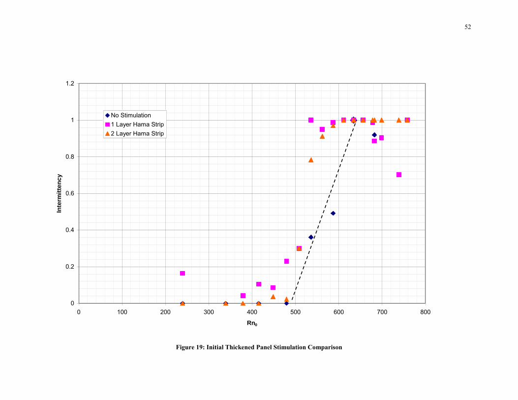
52

0

0.2

0.4

0.6

0.8

1

1.2

0 100 200 300 400 500 600 700 800

Rn

Inte

rmit

ten

cy

No Stimulation1 Layer Hama Strip2 Layer Hama Strip

Figure 19: Initial Thickened Panel Stimulation Comparison

• c---- • .. . r--------~------~------------. I ~ / =- ... t '---... ---,-------,-------r t t t .--+ / : •• t t

t t t ,' t . -----+-'/ '---.--,---------+-t -.i.----,----------1

:: t t I

I

t t t t t t / . t t I

I f--------~------~------~------~------~--, ----~------~-----

~

t t t t t • / • / r ' ~--- ~--- 1----r ~--- . ~-----c-. 1:------+-----r---:,' :-- ~--- ~-----

r A ~ [•i 6/ - ""'

53

The sizing tool estimated that the thickened panel needed a minimum of 0.041 inches of

thickness, or about 7-layers of tape. The appropriate sized strip was assembled and placed on the

model. The model was then rerun over the same range of speeds. The intermittency for the two

probes is tabulated below in Table 6.

Table 6: Intermittency Thickened Panel w/ 7-layer Hama strip Run Intermittency


0.5 0.00 0.00

1 0.00 0.00

1.25 0.00 0.00

1.5 0.00 0.00

1.75 0.00 0.37

2 0.00 0.86

2.25 0.05 1.00

2.5 0.89 1.00

2.75 0.96 1.00

3 1.00 1.00

3.25 1.00 1.00

3.5 1.00 1.00

3.75 1.00 1.00

4 1.00 1.00

4.25 1.00 1.00

4.5 1.00 1.00

4.75 1.00 1.00

5 1.00 1.00 The results for the 7-layer Hama strip were then also plotted on the same chart as the results for

no stimulation. The plot is featured below in Figure 20.

54

0

0.2

0.4

0.6

0.8

1

1.2

0 100 200 300 400 500 600 700 800

Rn

Inte

rmit

ten

cy

No Stimulation7 Layer Hama Strip

Δ Rn

Figure 20: Intermittency vs. Rn Thickened Panel w/ 7-layer Hama Strip

I ---I-

I I

I I I

I --+--

1 I

'~ --+----, ..... I I I

-r-•

55

Here, the results clearly show that the 7-layer Hama strip (the pink line) transitions at a lower

Rn value than the no-stimulation case (blue line). The effective difference in Rn is

approximately 100. Clearly the guidance based on empirical evidence is sound for providing a

stimulation thickness that effectively trips the flow.

The next step in the testing process was to see if a thicker Hama strip caused more of a

difference for the values of Rn where the flow transitioned. A 10-layer Hama strip was cut and

placed on the model, and the model was retested and reanalyzed. The intermittency results for

the 10 layer are listed in Table 7.

Table 7: Intermittency 10 layer Hama Strip Run Intermittency


0.5 0.00 0.00

1 0.00 0.00

1.25 0.00 0.00

1.5 0.00 0.32

1.75 0.02 0.79

2 0.08 0.96

2.25 0.42 0.99

2.5 0.99 1.00

2.75 1.00 1.00

3 1.00 1.00

3.25 1.00 1.00

3.5 1.00 1.00

3.75 1.00 1.00

4 1.00 1.00

4.25 1.00 1.00

4.5 1.00 1.00

4.75 1.00 1.00

5 1.00 1.00 The results for the 10-layer Hama strip were then plotted along with the 7-layer strip. Figure 21

below is the plot comparing 10-layer to 7-layer. The goal was to determine if the larger trip

would cause a greater shift in the value of Rn at which the flow transitioned.

56

0

0.2

0.4

0.6

0.8

1

1.2

0 100 200 300 400 500 600 700 800

Rn

Inte

rmit

ten

cy

10 Layer Hama Strip7 Layer Hama Strip

Figure 21: Intermittency vs Rn Thickened Plate (7 and 10 layer)

t t t I I t t J• I .... -o--o-.. ~ & A

j •,:-j -I I t t I I t t

I I

-----------------------------------,-1----------------------I

t t I

t t , ,

I I

--------------------------------,---t----------------------I

t t I

t t I I I

-------------------------------~---1----------------------I I

t t I

t t , I

t I I

t t l ~ ~ t t ..... ...... ...... t - - - - - -

57

Figure 21 demonstrates that having a thicker Hama strip does not cause there to be a

more significant difference in what value of Rn the flow transitions at. It can therefore be

concluded, based on the data collected from the thickened panel, that there is a certain optimal

thickness that at a minimum needs to be present in order to cause flow to transition from laminar

to turbulent at a lower value of Rn. It is not necessary to exceed this desired thickness as the

increased thickness has no positive affect on the lower Rn value. The greater thickness is

actually undesirable due to the increase in parasitic drag accompanying the thicker Hama strip.

58

6.1 Model Design and Mounting

The next stage of the project was to run tests and analyze the results of a “2-D” model.

The model is considered 2-D because it only has planar curvature; that is, the flow only changes

in the x and y directions. The 2-D model utilized for this project was designed and created based

on the Defense Advanced Research Projects Agency (DARPA) Suboff model. The Suboff model

is a generic submarine form developed by using two separate parabolic formulae for the bow and

stern sections (Stettler, 2009). The 2-D model created for this project took the bow and stern

formulae from the Suboff model and only applied it to the x and y plane. That is to say, looking

at the design from the waterplane view, straight down the z-axis, the model looks like the shape

outlined in Figure 22.

-2.5

-2

-1.5

-1

-0.5

0

0.5

1

1.5

2

2.5

0 0.5 1 1.5 2 2.5 3 3.5 4 4.5 5

Figure 22: Suboff Model Design

Length (ft)

Width (ft)

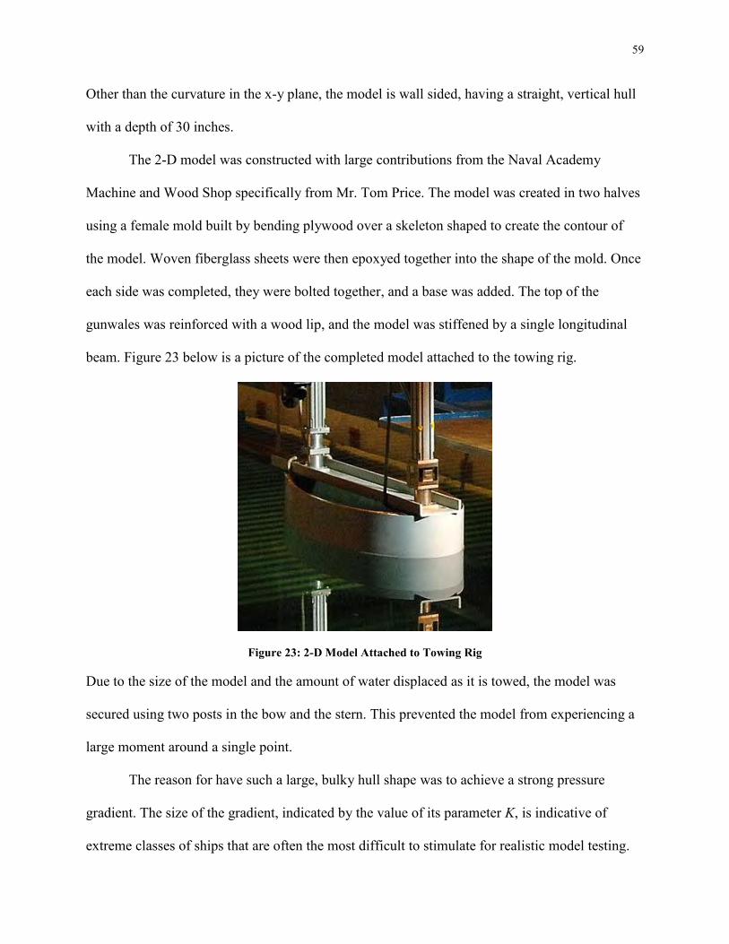
59

Other than the curvature in the x-y plane, the model is wall sided, having a straight, vertical hull

with a depth of 30 inches.

The 2-D model was constructed with large contributions from the Naval Academy

Machine and Wood Shop specifically from Mr. Tom Price. The model was created in two halves

using a female mold built by bending plywood over a skeleton shaped to create the contour of

the model. Woven fiberglass sheets were then epoxyed together into the shape of the mold. Once

each side was completed, they were bolted together, and a base was added. The top of the

gunwales was reinforced with a wood lip, and the model was stiffened by a single longitudinal

beam. Figure 23 below is a picture of the completed model attached to the towing rig.

Figure 23: 2-D Model Attached to Towing Rig Due to the size of the model and the amount of water displaced as it is towed, the model was

secured using two posts in the bow and the stern. This prevented the model from experiencing a

large moment around a single point.

The reason for have such a large, bulky hull shape was to achieve a strong pressure

gradient. The size of the gradient, indicated by the value of its parameter K, is indicative of

extreme classes of ships that are often the most difficult to stimulate for realistic model testing.

60

The extreme pressure gradient developed by the model can be seen visually at higher velocity

runs. Figure 24 below is a picture of the model being run at 4.5 fps.

Figure 24: 2-D Model Visual Pressure Gradient One can see that there is a distinct point at which the water goes from following the contours of

the model cleanly to becoming random and extremely chaotic. This point is at the thickest point

of the model and is where the pressure gradient transitions from positive to negative.

6.2 Analytical Analysis

It was established from testing the thickened panel model that a thick enough Hama strip

placed in the flow around a model would cause the water to behave as though it was moving over

the model at a higher velocity. The goal with the 2-D model was to confirm the results of the

thickened panel and then to determine if the pressure gradient had suppressed the flow and

forced the flow to relaminarize. If this was the case, the next step would be to determine at what

location fore to aft the effect of the trip was not influenced by the pressure gradient. The

hypothesis made at the beginning of the project was the optimal point to place a trip would be

when the pressure gradient parameter K was below a certain value. Figure 25 below represents

where that location may be on the applet outputs for the 2-D model.

61

-0.0002

0

0.0002

0.0004

0.0006

0.0008

0.001

0.0000 0.1000 0.2000 0.3000 0.4000 0.5000 0.6000 0.7000

% Length

K

Pressure Gradient Parameter, K

Estimation of threshold K value

Figure 25: 2-D Model Applet Output, K (2.5 fps)

t I f r-

I ' i I

I i I

I --

l- I l -:-

t I -

I i i - '-~ f--

~

~ ~ I ' i j f I - l r

62

The red arrow points to approximately where the pressure gradient, while still positive, was no

longer as extreme and therefore would allow for flow transitions without relaminarization. The

goal, then, in testing was to see if indeed such an optimal location could be found.

The first step in beginning testing on the 2-D model was the same as that for the

thickened panel. The hull form was entered into the programs available from Virginia Tech and

analyzed at the same range of velocities used for the thickened panel testing. The results for Rn

for each of the probe locations were recorded and are tabulated in below in Table 8.

Table 8: Rn Values Probe 2, 2-D Model Velocity (fps) Probe 2

0.5 138

1 195

1.25 218

1.5 239

1.75 258

2 276

2.25 293

2.5 308

2.75 324

3 338

3.25 352

3.5 365

3.75 378

4 390

4.25 402

4.5 414

4.75 425

5 434

It should be noted that as testing on the 2-D model began, it became apparent that the third probe

used for the thickened panel was no longer operating properly and was not considered in any

conclusions drawn from the 2-D model. Therefore, only one operational probe was available for

use during this phase of testing.

63

6.3 Experimental Analysis

The 2-D model was tested for five different conditions. The first of these was no

stimulation; this data set just as with the thickened panel would serve as the basis for

interpretation. The model was also tested with four different stimulation conditions. The first of

these conditions was to place a 7-layer Hama strip 1 inch in front of the probe (11 inches aft of

the bow or 18.3% of the length). The same sizing spreadsheet used on the thickened panel was

employed to approximate the thickness of the Hama strip for the 2-D model. Since the primary

focus of this second portion of testing was on K and strip location, 7 layers of tape were the

constant thickness for all stimulation placed on the 2-D model. For each data file collected from

tests done on the 2-D model, the same MATLAB code written for the thickened panel was

utilized to analyze the results. The results are listed below in Table 9.

Table 9: Intermittency for Initial 2-D Conditions Intermittency

Velocity (fps) No Trip 11 in aft

0.5 0.00 0.00

1 0.00 0.00

1.25 0.02 0.01

1.5 0.00 0.16

1.75 0.00 1.00

2 0.00 1.00

2.25 0.00 1.00

2.5 0.02 1.00

2.75 0.00 1.00

3 0.02 1.00

3.25 0.04 1.00

3.5 1.00 1.00

3.75 1.00 1.00

4 1.00 1.00

4.25 1.00 1.00

4.5 1.00 1.00

4.75 1.00 1.00

5 1.00 1.00

64

Once again intermittency was plotted vs. Rn. Figure 26 on the next page is a plot of the results

obtained from the no stimulation condition and with the trip 1 inch forward of the probe.

It is evident from the results plotted again that the 7-layer strip is effective in reducing the

Rn value at which the flow transitions for the 2-D model. This confirms the conclusion drawn

from the thickened panel. From here the next step was to determine how far forward stimulation

could be placed to still achieve turbulent flow.

65

0

0.2

0.4

0.6

0.8

1

1.2

050100150200250300350400450500

Rn

Inte

rmitte

ncy

7 Layer Strip (11 in aft)No Stimulation

Δ Rn

Figure 26: 2-D Comparison between Stimulation and No Stimulation

- ---- ---- --- - -~ ~ . ... -· ·- - - _.. -~ .. - -

~

. ~ ~ +- +- +- I ~ ~ ~

t t Hl1 . t t t I

I

r------r------r------.-r------------~---------r------r-----------

~ ~ ~ I ~ ~ I ~ ~ -1- -1- -1- ..... . -1- -1- -1- -1-

t t I

t t t t I

~ ~ t- t- t- t- 1 t- t- t- t- ~ f .. .. .. I .. .. I --r------ r--· --r------r---

I t t " • .. ,. ,. I .. .. I

.. .. +- +- +- i l . . r +-

I II . d t t t t I I

~ ~ ~ I ~ ~ I

--r--- • --r------r---~ ~ ~ I ~ ~

~ ~ t- t- t- I t- t- t- t-

t t t t t .. .. +- +- +- I . +- +- +- +- I

.. .. I .. .. I

--r----___t- r--- • --r------r---.. .. I .. .. I

f I I

t I

t t t t ~ ~ -1- -1- -1- I -1- -1- -1- -1- -1-I

.. .. ,. I .. .. I ---- __ .. .... .... .... .... +- .... r--- ---- ·-----· ................ ...... ..... -------r--- -· -r ~ ~ ~ ~ ~

~ ~ t- t- t- t- t- t- t- t-

I I I I -. -

.. .. +- +- +- +- +- +- +- +-

t t t t t ~ ~ -1- -1- -1- -1- -1- -1- -1- -1-

66

The next phase of testing began by placing a 7-layer Hama strip at a distance of 10% of

the model length aft of the bow (6 in aft). 10% is considered to be the fall-back position for

placing stimulation on ship-models. After the model was tested with stimulation at 6 inches aft of

the bow, it was also tested at 4 inches aft and 8 inches aft of the bow. The data collected was all

analyzed, and the results for the last three conditions are tabulated below in Table 10.

Table 10: Intermittency 2-D Model Stimulation Cases Intermittency

Velocity (fps) 6 in aft 4 in aft 8 aft

0.5 0 0 0.0261

1 0.0291 0 0

1.25 0.1925 0.01 -

1.5 0.7916 0.0496 0.7358

1.75 0.973 0.8803 -

2 1 1 1

2.25 1 1 -

2.5 1 1 1

2.75 1 1 -

3 1 1 1

3.25 1 1 -

3.5 1 1 1

3.75 1 1 -

4 1 1 1

4.25 1 1 -

4.5 1 1 -

4.75 1 1 -

5 1 1 -

Once all the data was compiled, more plots were made and conclusions were drawn from these

plots. The plot for all the 2-D model stimulation conditions is below in Figure 27.

67

0

0.2

0.4

0.6

0.8

1

1.2

0 50 100 150 200 250 300 350 400 450 500

Rn

In

term

itte

ncy

11 in aft6 in aft4 in aft8 in aftNo Stimulation

Δ Rn

Figure 27: Intermittency vs. Rn for all 2-D Stimulated Conditions

I I t t d( • • .. • ••

• q1 -. -t t

--- --- --- ---

t t t I t I I

--- ---

I

t t t I

t I I I I

--- --- --+-I I

t t t I

t : t t I I I I

I

t I

t I

68

The striking result that can be seen from the plot in Figure 27 is that there was no

significant difference in the effect of the trip based on the longitudinal position of the Hama

strip. The significance of this is more aptly put in terms of the pressure gradient parameter K.

Table 11 below is a listing of the K values at all the stimulation locations at 2.5 fps.

Point aft (in) K 4 0.000158 6 9.89E-05 8 6.42E-05

11 3.05E-05 Table 11: K Values for Tripped Conditions

The values of K at which each Hama strip was placed is greater than the value at which it was

hypothesized that stimulation would have to be placed in order to over come the effect of the

pressure gradient on the flow. It also should be noted that again the Rn values at which the flow

transitioned were much lower than the hypothesized value. Indeed, the values for the 2-D were

less than those for the thickened panel, which is not what would be expected. Based on the

results from the 2-D model, one could conclude that the location of the strip is not a large factor

in tripping the flow; however, this conclusion does not align with previous testing results.

Further discussion of why this conclusion holds true for this project is found in section 7.1.

Unfortunately, during the testing of the 2-D model the last probe that was available for

use on the project stopped functioning, meaning further testing and comparisons were not

possible. The probes used posed numerous problems over the course of the project. Three of the

original probes that were inherited from previous projects were never able to provide reliable

data, and the three other probes that were acquired over the course of the project all failed either

due to human error (stripping of wires, e.g.) or due to the testing environment. While the sensors

are meant to be used in air or water, it could have been that the condition of the water in the

towing tank and the process of taking the probes in and out of the water may have contributed to

69

the short lifetime of some of the sensors. That, however, in and of itself is a lesson learned from

this experiment. Using a hot-film anemometer system is a means to determine whether or not

flow is laminar, transitional, or turbulent. However, due to the sensitivity of the probes, the high

cost of the probes, and the difficulty in achieving replicable results, another avenue of research

and testing may need to be considered in the future.

70

7. Conclusions and Recommendations for Future Work

The extent and depth of this project must be considered in order to fully comprehend the

results and conclusions given. 342 data files were collected over the course of this project,

totaling about 250 total runs in the towing tank, or about 23 total miles of model towing. From

all these runs and data files, several significant conclusions were drawn and are discussed below:

Flow transition can be characterized by Rn and K. The majority of work and research

done with these parameters up to this point has been focused on testing in a wind tunnel.

It was a novel approach to apply these parameters to testing done in a towing tank, and

the work done in this project confirms that these values do characterize the flow around a

model. All the tests run on the thickened panel and the 2-D panel show that the flow can

be accurately described used Rn and K.

Differentiation between laminar and turbulent flow. As mentioned in Section 2.7, MIDN

Islin laid out some of the ground work for this project with her own research performed

in 2007. However, at the onset of this project the value of her data collection methods

was unknown. After major analysis of the data collected from this project, it was found

that using the hot film probes proved very valuable. The analysis of each signal proved

time consuming as well. The code discussed above in Section 5.3 was able to be used for

all data files collected; however, these files could not be analyzed in bulk. Each signal

had to analyzed and then visually checked to ensure that the result made sense. It was

necessary to scrutinize each output before plotting results and drawing conclusions.

However, this level of scrutiny proved that not only can one differentiate whether the

flow is laminar or turbulent but one can tell exactly how far between laminar and

turbulent the flow is when transitioning. The intermittency of each signal can be

71

measured to tell whether the flow is early in the transition phase or further along. These

results can be extrapolated to determine the earliest velocity at which transition occurs.

Measuring the effect of a stimulator on the flow. As mentioned above, the purpose of a

turbulence stimulator, such as the Hama strips used in this project, is to induce a

momentum jump in the flow. This jump is characterized by the flow beginning to

transition at a lower Rn value. The results from the thickened panel and the 2-D model

indicate that the momentum jump induced by a 7-layer Hama strip is about 100. The goal

is to find the smallest amount of stimulation that will produce the largest momentum

jump. The steps and application of the methods used in this project allow for the

measurement of the momentum jump for various types and sizes of turbulence

stimulators.

Optimizing location of turbulence stimulator. Based on the results of the effectiveness of

a given stimulator, one can use the Applets and the discussions above to see where the

trip can be placed in order to cause the flow to transition. Viewing the results of natural

transition for a given ship-model and coupling those results with the measure of

effectiveness for a given trip, one can determine the farthest location forward along the

hull where the trip can be placed to cause the earliest transition.

Determining untrippable velocities. Based on the results of both the thickened panel and

the 2-D model testing, it is evident that there is an optimal size for a turbulence stimulator

that will cause the flow to transition at a lower Rn value. It is also evident that there are

certain speeds at which no size stimulator will cause the flow to transition. The presence

of the stimulators causes the flow to trip at an Rn value about 100 times less than the

value required for no stimulation. However, there is still a minimum value that must be

72

achieved before transition occurs. For the 2-D model this minimum value was 250. Thus,

one can take any hull form, analyze the shape using the applets discussed above, and, if

the Rn value in addition to the jump of 100 provided by a trip is less than 250, the flow

will not transition. The significance of this is that a naval architect can tell if testing a

given velocity on a certain model will be productive or not. For instance, the USS

Constitution model was tested at speeds often as low as 0.5 fps. The use of the applets

would tell researchers the feasibility of tripping the flow at that velocity. The results

indicate that while further research and testing is necessary to optimize turbulence

stimulation, the testing limitations and constraints for a given model can be more clearly

defined.

Future research and work will only further expound on the conclusions discussed above.

There are several areas of interest that still need to be concentrated on in order to further the

results featured here. As mentioned above in sections 5.4 and 6.3, the values of Rn for both the

thickened panel and 2-D model at which the flow transitioned were much lower than the

hypothesized threshold of 800. There are multiple possible reasons why this may be the case for

each model. One explanation could be the difference in facilities where testing was occurring.

The threshold value of 800 was primarily based on information and data collected from work

done in a wind tunnel. The fact that all these tests were done in a towing tank may have

contributed to the difference. The turbulence of the water in the tank prior to each test most

likely had a large impact on the results. After a test run, the water on the surface settles relatively

quickly. However, the amount of sub-surface turbulence remains for a sustained period after a

single run. In a wind tunnel, the air is passed through a series of flow management devices in

73

order to produce an “ideal” medium for each test. Ship-model testers do not have such a luxury.

A model tester will generally use the level of turbulence on the surface as the gauge for when to

begin the next run. One could wait between runs for the water in a tow tank to completely settle,

but this process could take hours. It is not economically feasible to conduct tests in this way; runs

must be made when the water is still disturbed. Thus, while the results seem to not follow the

initial assumptions made, they may more closely represent what one should expect when

conducting ship-model testing.

In similar fashion, one would have expected the values of Rnat which the 2-D model

transitioned to be greater than those for the thickened panel. However, as the results indicated

above, the values for the 2-D model were in fact less. A possible explanation for this occurrence

would be the size difference between the two models. Because the 2-D model displaced so much

more water than the thickened panel, the amount of disturbance caused in the tow tank may be

that much greater as well. Since the same interval of 30 seconds was kept between runs for both

models, the water may have been more chaotic for each 2-D run and thus more prone to tripping.

The sensors on the model are located with 2 feet of the surface, thus another possibility is that

the effects on the surface caused by the large model may be detected by the sensors. These

occurrences should be explored in depth prior to conducting any furthering testing.

Significant strides were made for future research and work. This project began with the

overall goal of exploring a “novel” approach to turbulence stimulation. The novelty of the

approach was to use analytical means to determine the ideal size and location of a stimulation

device. The ultimate output from this project and future research will be to have a universal

analytical tool that can take inputs from a given model and optimize turbulence stimulation for

that model. As mentioned above, to achieve this end state, further testing and analysis must be

74

done on the models used in this project and on actual ship-models.

Ultimately, the biggest step forward is to begin conducting similar testing on an actual

ship-model. It had been discussed in the proposal for this project that testing would be done on

the model of the USS Constitution. The reasoning for this was that the Constitution’s hull form is

challenging due to its bulk similar to that of the 2-D model. However, at this stage testing on any

ship-model will lead to more positive results and more definite conclusions. The way ahead is

promising, large strides have been taken in right direction, and the positive results of this project

are sure to be followed by more.

75

References

Dantec Dynamics, A/S. “Flush mounted hot-film probe (55R45 and 55R46).” 2010

<http://www.dantecdynamics.com/Default.aspx?ID=757>.

Devenport, William and Joseph Schetz. engAPPLETS. Version 1.0 28 Aug. 1998

<http://www.engapplets.vt.edu>.

Gibbings, J.C., O.T. Goksel, and D.J. Hall. “The Influence of Roughness Trips Upon Boundary-

Layer Transition: Part 1 Characteristics of Wire Trips.” Aeronautical Journal 898.90

(1986): 289-301.


Layer Transition: Part 2 Characteristics of Single Spherical Trips.” Aeronautical Journal

899.90 (1986): 357-367.


Layer Transition: Part 3 Characteristics of Rows of Spherical Transition Trips.”

Aeronautical Journal 900.90 (1986): 393-398.

Gillmer, Thomas C. and Bruce Jonson. Introduction to Naval Architecture. Annapolis, MD:

United States Naval Institute, 1987, 209, 217.

Hama, Francis R., James D. Long, and John C. Hegarty. “On Transition from Laminar to

Turbulent Flow.” Journal of Applied Physics 28.4 (1957): 388-394.

Hughes, G. and J.F. Allan. “Turbulence Stimulation on Ship-models.” 1951.

Islin, Rebecca L. “Turbulent Flow Stimulation on a Thickened Panel: An Investigation of

Turbulence Stimulation Devices.” EN496 report, United States Naval Academy, 2007.

http://www.engapplets.vt.edu/

76

Lee, T. and S. Basu. “Measurement of unsteady boundary layer developed on an oscillating

airfoil using multiple hot-film sensors.” Experiments in Fluids. New York, NY:

Springer-Verlag, 1998.

Moran, Michael J, Howard N. Shapiro, Bruce R. Munson, and David P. DeWitt. Introduction to

Thermal Systems Engineering: Thermodynamics, Fluid Mechanics, and Heat Transfer.

John Wiley & Sons, Inc, 2003.

Munson, Bruce R., Donald F. Young, and Theodore H. Okiishi. Fundamentals of Fluid

Mechanics. 5th ed. John Wiley & Sons, Inc, 2006.

Ridgely-Nevitt, Cedric. “The Resistance of Trawler Hull Forms of 0.65 Prismatic Coefficient.”

Society of Naval Architects and Marine Engineers: Transactions, 1956, 433-445.

Ridgely-Nevitt, Cedric. “The Resistance of a High Displacement-Length Ratio Trawler Series.”

Society of Naval Architects and Marine Engineers: Transactions, 1967, 426-468.

Schetz, Joseph A. Boundary Layer Analysis. New Jersey: Prentice-Hall, Inc., 1993.

Schneider, S.P. “Improved Methods for Measuring Laminar-Turbulent Intermittency in Boundary

Layers.” Experiments in Fluids. New York, NY: Springer-Verlag, 1995, 370-375.

Stettler, Jeffery. Personal Interview. 29 April 2009.

van Manen, J.D. and P. van Oossanen. “Resistance.” Principles of Naval Architecture. Vol. 2.

Ed., 53.

Volino, Ralph J., Michael P. Schultz, and Christopher M. Pratt. “Conditional Sampling in

Transitional Boundary Layer Under High Freestream Turbulence Conditions.” Journal of

Fluids Engineering, 2003, 1-3.

Waltman, Charles II. “Low-Speed Performance Characteristics of a Full Bodied Sailing Vessel.”

EN495 Report, United States Naval Academy, 2003.

A-1

Appendix A – Steps For Using ThermalPro Software

The steps for using the IFA300 ThermalPro software are as follows:

1. System start-up

a. Ensure the IFA300 unit is turned on, the on/off switch is located in the back

left corner of the unit.

b. Connect probes to the appropriate IFA300 channels using BNC cables.

i. There are eight possible connection ports, so ensure you begin in

numerical order, probe 1 connects to channel 1, etc.

c. Ensure the attached PCU is turned on and logged into. The automatic login

screen that comes up can be utilized by pushing enter at start-up. Once the

computer is up and running, the ThermalPro software must be opened.

i. There are two versions of ThermalPro on the computer; one is an

outdated version. However, the outdated version cannot be uninstalled

without affecting the newer version. To open the newest version, pull

up the start menu, select the Programs tab, and then ThermalPro. The

program labeled ThermalPro v. 4.6 is the older version. It should also

be noted that the ThermalPro shortcut on the desktop is for the older

version and cannot be modified to open the new version.

2. Probe inputs

a. To begin, one must access the probe table, which can be found under the

acquisition tab as indicated in Figure 28 below.

A-2

Figure 28: ThermalPro Home Screen

b. Press the blue Get File icon on the right side of the window to bring up a list

of probes already inputted into the system. Select the option labeled

sfilm3.R0001. This will open a table of three film sensors as seen below in

Figure 29.

Probe Table command under Acquisition Tab

A-3

Figure 29: ThermalPro Probe Table

c. Each preloaded probe must be modified to represent the actual sensor that is

being plugged into the system.

i. Double click on each probe to adjust the input options under the

Sensor Setup box.

1. The IFA channel number must first correspond to the terminal

that the probe is plugged into in the rear of the system.

2. The cable resistance should either by 0.33 Ω or 0.3 Ω

depending on the length of the cable connected to the probe. A

longer cable requires the higher resistance.

Generic Probe Files found here

A-4

3. The probe resistance is read by the system and cannot be

changed or modified.

4. The Opr Resistance or operational resistance is the resistance

required for the probe to function. This value is provided with

each probe, but the actual resistance may need to be adjusted

throughout test runs as it fluctuates to accommodate for

changes to the sensor through overuse, time, or other external

factors.

5. The offset is adjusted to have the probe read 0 volts when

stationary with no flow over its surface. Attach the output from

the IFA system directly to a voltmeter and then adjust the

offset up or down until the voltmeter is reading approximately

0.

6. The gain serves to amplify the signal put out by each probe.

The goal is have a high enough gain to be able to visually read

each signal.

ii. Table 12 below contains all the values that were inputted for the

probes utilized in this project.

Table 12: Probe Inputs for ThermalPro Probe Table Probe 1 Probe 2 Probe 3

Cable Res. = 0.33 Ω

Cable Res. = 0.3 Ω

Cable Res. = 0.3 Ω

Opr Res. = 20 Ω Opr Res. = 15 Ω Opr Res. = 17 Ω Offset = 0.78 V Offset = 1.1 V Offset = 1.75 V

Gain = 10 Gain = 5 Gain = 5

A-5

iii. After each probe has all values inputted, selecting the save line button

will lock the values in for that probe.

3. Engaging Probes and Saving the Probe Table

a. Select the green Next Screen button in the lower right corner of the screen

seen in Figure 29.

i. Probes will engage and the acquisition screen seen below in Figure 30

will pop up.

Figure 30: ThermalPro Acquistion Screen

ii. From this point forward the probes will remained turned on until the

screen is closed and/or the system is shut down. It should be noted that

A-6

one must turn off the probes before removing from the water in order

to prevent overheating.

b. Select the green Next Screen button to bring up the screen seen below in

Figure 31.

Figure 31: ThermalPro Output Screen

c. Select the green Trigger button in the bottom right corner of the screen.

A-7

i. Selecting this will cause the computer to “run” the probes for a brief

amount of time and then bring up the small window seen below in

Figure 32.

Figure 32: ThermalPro Final Save Screen

d. Select Ok and the system will return to the screen pictured in Figure 30.

i. The probes will still be turned on and the data inputted into the probe

table will be saved.

B-1

Appendix B – MATLAB Code for Analyzing Data

clear all load file339.txt data=file339; t=data(5001:30000,1); tau1=data(5001:30000,4); tau2=data(5001:30000,5); tau3=data(5001:30000,6); n=length(t); [B,A] = butter(9,10/500,'high'); tau1_filt=filtfilt(B, A, tau1); tau2_filt=filtfilt(B, A, tau2); tau3_filt=filtfilt(B, A, tau3); tau1floor=ceil(floor(abs(tau1_filt)/0.12)/1000); tau2floor=ceil(floor(abs(tau2_filt)/0.05)/1000); tau3floor=ceil(floor(abs(tau3_filt)/0.08)/1000); %plot(t,tau2_filt) %figure %plot(t,tau3_filt) %figure %plot(t,tau2floor) %figure %plot(t,tau3floor) %figure tau1new=ceil(abs(tau1floor.*tau1_filt)); tau2new=ceil(abs(tau2floor.*tau2_filt)); tau3new=ceil(abs(tau3floor.*tau3_filt)); tau1new_prime=gradient(tau1new,t); tau2new_prime=gradient(tau2new,t); tau3new_prime=gradient(tau3new,t); index1=find(tau1new_prime~=0); index2=find(tau2new_prime~=0); index3=find(tau3new_prime~=0); dindex1=diff(index1); dindex2=diff(index2); dindex3=diff(index3); lamindex1=find(dindex1>250); lamindex2=find(dindex2>250); lamindex3=find(dindex3>250); lamindex1=lamindex1+1; lamindex2=lamindex2+1; lamindex3=lamindex3+1; if isempty(index1)==1

B-2

int1(1:n)=0; else int1(1:index1(1)-1)=0; end if isempty(index2)==1 int2(1:n)=0; else int2(1:index2(1)-1)=0; end if isempty(index3)==1 int3(1:n)=0; else int3(1:index3(1)-1)=0; end if isempty(index1)==1 int1(1:n)=0; elseif isempty(lamindex1)==1 int1(1:n)=1; else int1(index1(1):index1(lamindex1(1)-1))=1; end if isempty(index2)==1 int2(1:n)=0; elseif isempty(lamindex2)==1 int2(1:n)=1; else int2(index2(1):index2(lamindex2(1)-1))=1; end if isempty(index3)==1 int3(1:n)=0; elseif isempty(lamindex3)==1 int3(1:n)=1; else int3(index3(1):index3(lamindex3(1)-1))=1; end if isempty(index1)==1 int1(1:n)=0; elseif isempty(lamindex1)==1 int1(1:n)=1; else

B-3

for i=1:length(lamindex1)-1 int1(index1(lamindex1(i)-1):index1(lamindex1(i))-1)=0; int1(index1(lamindex1(i)):index1(lamindex1(i+1)-1))=1; end end if isempty(index2)==1 int2(1:n)=0; elseif isempty(lamindex2)==1 int2(1:n)=1; else for i=1:length(lamindex2)-1 int2(index2(lamindex2(i)-1):index2(lamindex2(i))-1)=0; int2(index2(lamindex2(i)):index2(lamindex2(i+1)-1))=1; end end if isempty(index3)==1 int3(1:n)=0; elseif isempty(lamindex3)==1 int3(1:n)=1; else for i=1:length(lamindex3)-1 int3(index3(lamindex3(i)-1):index3(lamindex3(i))-1)=0; int3(index3(lamindex3(i)):index3(lamindex3(i+1)-1))=1; end end if isempty(index1)==1 int1(1:n)=0; elseif isempty(lamindex1)==1 int1(1:n)=1; else int1(index1(lamindex1(length(lamindex1))):index1(length(index1)))=1; int1(index1(length(index1))+1:n)=0; end if isempty(index2)==1 int2(1:n)=0; elseif isempty(lamindex2)==1 int2(1:n)=1; else int2(index2(lamindex2(length(lamindex2))):index2(length(index2)))=1; int2(index2(length(index2))+1:n)=0; end

B-4

if isempty(index3)==1 int3(1:n)=0; elseif isempty(lamindex3)==1 int3(1:n)=1; else int3(index3(lamindex3(length(lamindex3))):index3(length(index3)))=1; int3(index3(length(index3))+1:n)=0; end %plot(t,tau1) %hold on %plot(t,int1,'r') %figure %plot(t,tau2) %hold on %plot(t,int2,'r') figure plot(t,tau3) hold on plot(t,int3,'r') interfract1=length(find(int1==1))/n interfract2=length(find(int2==1))/n interfract3=length(find(int3==1))/n

REPORT DOCUMENTATION PAGE Form App ro ved … · REPORT DOCUMENTATION PAGE Form App ro ved OMB N o....

Documents

Transcript of REPORT DOCUMENTATION PAGE Form App ro ved … · REPORT DOCUMENTATION PAGE Form App ro ved OMB N o....