Replies to Reviewer Comments - CP - Recent

David Wade on behalf of the authors 1 of 25

Replies to Reviewer Comments David Wade on behalf of the authors

We would like to extend our gratitude to Jim Kasting and the anonymous reviewers for the time and care they took in reviewing the paper. The comments will be dealt with in turn and changes to the updated manuscript will be described. In all cases, reviewer comments can be identified by the red text and the author reply in the black text. We’ve provided a tracked changes document for the editor where the new additions (bold black text here) are added in blue and text we have deleted is scored out in red for clarity.

Jim Kasting This paper describes an exhaustive study of the effects of changing pO2 on Phanerozoic climates. The calculations are carried out with two different state-of-the-art climate models, one of which is an Earth system model that includes coupling between the atmosphere and the biota (forests in particular). This paper responds to a disagreement between the original 3-D climate simulations by Poulsen et al. (2015) and subsequent 1-D simulations by Goldblatt (2016) and Payne et al. (2016) (the latter of which is my own research group). The Poulsen et al. model predicted that higher pO2 leads to lower surface temperatures; the two 1-D models predicted just the opposite. The new paper basically agrees with the 1-D models, i.e., high pO2 leads to higher surface temperatures. But the results are more complicated. High pO2 can actually lead to lower surface temperature when the starting state is a warm climate. In general, the calculations seem to be well done, and the results are well described. I have a few minor comments below. But this paper should be useful in close to its present form. The basic conclusion, which is restated in point 4 below, is that changes in pO2 are secondary drivers of Phanerozoic climate. The main driver is changes in pCO2, and also in solar luminosity, which is not mentioned too many times explicitly but which is implicit in the calculations. 1. (p. 3, l. 2) ‘Indeed, there is support for elevated O2 by carbon isotope measurements (Beerling et al., 2002).’–Elevated O2 during what time period? We thank Prof. Kasting and have added the following to clarify: “... isotope measurements during the Permian (Berling et al., 2002).” 2. (p. 9, l. 1) ‘Proxy data for the Maastrichtian was obtained..’ –Proxy data..were obtained. (‘Data’ is plural.) This same mistake is found elsewhere. Thanks for spotting this. We have changed this in the text on P9 line 1, P9 line 3, P24 line 20. 3. (p. 19, l. 18) ‘The changes in terrestrial carbon storage are equivalent to 56% of the atmospheric CO2 content in the Asselian and 16% in the Wuchiapingian which suggests that pO2 induced Earth system feedbacks could have significant impacts on


atmospheric pCO2.’ –No, I don’t buy this argument. Think of the numbers and the relevant time scales. Today, the atmospheric CO2 reservoir is about 1/60th the size of the dissolved inorganic carbon (DIC) reservoir in the ocean. On long time scales (> 0.5 m.y.), what changes is the total CO2 content of the combined atmosphere-ocean system. Sequestering 56% of atmospheric CO2 in forests is a trivial change to this combined reservoir. Forests can only directly affect atmospheric CO2 if they are chopped down or regrown on very short time scales, less than the time required for the atmosphere and ocean to equilibrate. We take Prof. Kasting’s point here. In our study we neglected to simulate ocean biogeochemistry and as a result there are issues in interpreting the effects of changes in pO2 on the carbon cycle. In light of this and the other comments from the reviewers we suggest to leave the section on Earth system feedbacks in (section 3.4) but with some modifications to the text. As a result we have modified the text and deleted lines 18 and 19 on P19 and lines 1 and 2 on P 20 and added the following (in bold): “Note that while the atmosphere and vegetation are coupled in the physical sense, the carbon cycle is not interactive so determining the impacts of atmospheric pO2 on the carbon cycle remains an outstanding problem.” 4. (p. 27, l. 11) ‘pO2 therefore remains a secondary contribution to climatic variability in the Phanerozoic but most likely to be important during the Permian.’ –The first part of this statement is essentially what we said in the conclusion section of Payne et al. (2016): ‘Given the large uncertainties in past levels of both O2 and CO2, we agree with Berner [2006] that Phanerozoic climate has been driven largely by changes in atmospheric CO2 and solar luminosity, coupled with changes in continental geography.’ So, we are in fundamental agreement on this question. We thank Prof. Kasting for the comment and have added the following text to clarify this point: “pO2 therefore remains a secondary contribution to climatic variability in the Phanerozoic in agreement with Payne et al. (2016) but most likely to be important during the Permian.” 5. (p. 27, l. 17) ‘If pCO2 and pO2 are intimately linked such that cooler climates tends to increase pO2 this would suggest that pO2 responses have helped to prevent Snowball Earth initiation in the Phanerozoic.’ –Cool! I like this result. The effect of pO2 on climate is not strong, but it may help to prevent Phanerozoic Snowball Earth events. Thank you for the comments, we agree this is indeed an interesting result. Jim Kasting Penn State


Anonymous Reviewer #2 Wade et al. quantify the climatic impact of changing atmospheric oxygen concentrations (pO2) using two ocean-atmosphere general circulation models in the Holocene, the Cretaceous and the Permian. They systematically conduct their simulations at 3 pO2 levels (10, 21 and 35 ‰), which are shown to reasonably cover the pO2 changes reported during the Phanerozoic. In their model, higher pO2 values (and associated greater atmospheric mass) lead to two competing effects: an increase in Rayleigh scattering that induces an increase in albedo and surface cooling, and an increase in greenhouse effect that leads to surface warming. The authors first run the two models on the preindustrial Holocene configuration. Interestingly, the state-of-the-art IPCC-class model (HadGEM-AO) and the version of the model designed for deep-time studies (HadCM3-BL) provide climatic responses that agree at first-order, thus supporting the robustness of the subsequent deep-time HadCM3-BL integrations. In their Holocene simulations, the mean annual global climate response to an increase in pO2 is a warming, with varying regional patterns. The warming is particularly strong in the northern high latitudes, especially during the cold month. A cooling is simulated at low latitudes, which is especially strong and extends to most continental areas during the warm month. Higher pO2 values tend to flatten the equator-to-pole temperature gradient. They also lower the climate sensitivity to atmospheric carbon dioxide. Then the authors run the HadCM3-BL model in the Cretaceous and two Permian time slices. They show similar climatic behaviors and discuss two specific points related to each case study: the response of the terrestrial vegetation to changing O2 levels during the Permian and the impact of changing O2 levels on the capacity of their model to simulate the low latitudinal temperature gradients traditionally reconstructed for the Cretaceous based on proxy data. They notably show that changing oxygen concentration only slightly improves model-data agreement in the Maastrichtian. Last but not least, they propose a quantification of the uncertainty in global temperature resulting from uncertainties in the pO2 during the Phanerozoic. They show that the temperature bias associated with poorly constrained pO2 levels is significantly lower than the uncertainty associated with the lack of constraints on the pCO2, with a notable contribution of pO2 during the Permian though. It should be noted that Wade et al.’s implementation of O2 forcing leads to results that agree at firstorder with most previous attempts, but differ in sign with the simulations of Poulsen et al. (2015; 10.1126/science.1260670). Analysis of the model runs led the authors to suggest that Poulsen et al.’s implementation may not be totally coherent. We would like to thank the reviewer for their time in providing such an in depth review of our manuscript and for their comments and suggestions on how to improve it. I think that Wade et al. provide a very interesting and innovative study that shades new light on the poorly explored question of the potential impact of changing pO2 levels on deep-time climate. The results are based on numerous general circulation model simulations using two generations of climate models. The manuscript is relatively well organized (an exception if the methods section, see comments) and richly illustrated with high-quality figures and abundant information embedded in tables. The manuscript is lengthy (as testified by the length of my summary above). This is essentially due to the large amount of diagnostics


provided by the authors but I also suggest below deleting the section of the manuscript relative to the impact of wind stress, which I think is not very useful and relatively badly integrated in the manuscript (see hereafter). We thank the reviewer for this comment. This is also suggested by reviewer #3 and we agree that removing this from the paper will help make the overall messages clearer. The discussion of the discrepancy with Poulsen et al.’s (2015) results is well conducted. Indeed, Wade et al. not only compared their results with the diagnostics provided by Poulsen et al. but also downloaded and analyzed the climatic simulations of the latter, by repeating key diagnostics that they previously provided for their own model runs. This effort deserves to be acknowledged. As a reviewer of this paper, I would be happy to have Poulsen et al.’s response, be it as another review or at least as a comment on the ClimPast Discussion forum. Therefore, I encourage the Editor to contact Poulsen et al. I also encourage the authors to make their implementation of O2 forcing available online (as numerical – fortran – code or as equations) in order to allow other research groups to conduct similar experiments using other climate models, thus permitting to determine to what extent the discrepancy between Poulsen et al.’s results and theirs is model-dependent (and conversely, implementation-dependent; see major comment). We thank the reviewer for the comments and suggestions for us to provide some numerical code or equations to help others. We did consider this at length but after consideration we feel that this would end up not being useful beyond users of the specific climate models we have used in this study. We will make clear in the manuscript that users of the versions of the climate models we have used are welcome to our code changes, upon request, but these changes are so specific to our models that they would not prove useful to other modelling groups. Indeed, implementing the changes in HadGEM3-AO was very different to implementing the changes in HadCM3-BL. Added to the Code and data availability section: “Readers who would like advice on how to implement alterations to pO2 in their climate model are encouraged to contact the corresponding authors. UM users can obtain the code changes for these particular versions from the corresponding authors.” Most of my comments are intended to help the authors sharpen and clarify their manuscript. The only (other) major (potentially critical) comment I have regards the robustness of the analyzed climatic simulations. I suggest accepting this manuscript with moderate revisions, provided that Wade et al. can demonstrate that their climatic simulations are robust (i.e., sufficiently close to equilibrium). Please note that the text refers in several places to supplementary figures. I did not find any SOM. We thank reviewer #2 for pointing this out and this was an error at the submission stage we will rectify in the response. A. Major comments: • On the discrepancy with Poulsen et al.’s results. Since the current study casts doubts about the Poulsen et al. implementation of O2 forcing, I suggest making the implementation of Wade et al. available online to allow other modelers to repeat such experiments using


alternative climate models – using GENESIS in particular. I think that such common effort will allow improving the implementation of oxygen forcing in a collaborative and efficient way. As we have alluded to above we don’t feel that this would be a practical action going forward. Instead, we would be very willing to help others with implementing the code changes required to repeat the calculations we have performed in their own models. Indeed, the formulation of equations used in different climate models may make it deeply difficult, if not nigh impossible, to perform these types of simulations. As we mentioned above, the code changes we made in the two different versions of the Hadley centre climate model were drastically different. • On the robustness of the climatic simulations. I recently had the opportunity to attend a presentation by Dan Lunt showing that the climatic simulations published by Lunt et al. (doi:10.5194/cp-12-1181-2016), run for 1422 years, did not reach equilibrium. A longer duration in the order of 10 kyrs is necessary to reach deep-ocean equilibrium, with the global mean SST simulated at the end of the longer simulation significantly differing (several °C) from the SST simulated after 1422 years of model integration time. Therefore I logically wonder if the climatic results used in the present manuscript based on the 1422-year long model integrations (see page 6, line 15) can be trusted. To what extent are the model runs equilibrated? I encourage the authors to clarify this point. Otherwise, the subsequent publication of longer model runs may significantly question the robustness of this entire study. We thank the reviewer for this comment, which touches on an important issue in climate modelling more widely. We reject the idea that the simulations we have shown are not sufficiently well spun up to allow us to make robust conclusions. The desirable length of a particular climate model integration depends intrinsically on the question being asked and on a number of factors including:

● Model components (e.g. inclusion of land ice would lead to a longer integration time due to the response time of that physical system)

● Magnitude of the imposed changes (with respect to the baseline state) ● Pragmatics (time and computational resources required to perform the integration)

The main question we ask here is how does the climate simulated by the models we’ve investigated, and by proxy the Earth, respond to changes in the amount of O2 in the atmosphere. This is a form of a forcing-feedback study in which the forcing is being imposed by changing pO2 in our climate models. Forcing-feedback studies are widely used for example to understand how climate change will evolve over the coming century. Ultimately we are trying to understand if the signal from the forcing is large or is within the internal noise present in the chaotic climate system. We believe we have robustly shown the amount of climate change from changing the amount of pO2 in the atmosphere is second order compared to changes in pCO2 but is not insignificant and we believe we have identified the major mechanisms behind the changes in climate. However, we wish to further elaborate on why we feel these simulations are robust. Hereafter e will refer to the doi:10.5194/cp-12-1181-2016 study as Lunt et al. 2016. Model Components While the deep ocean does take a considerable amount of time to spin-up, the interest of our study is much more in the shallow ocean response to the imposed changes. Indeed, one


simulation passing some ocean bifurcation and entering into a new pattern of circulation after several thousand model years would be an intriguing result but would not be insightful for our understanding of the impact of atmospheric pO2 changes. It is worth noting that on long enough time periods, orbital changes would need to be accounted for as these are not fixed on timescales of 10 kyr so would ideally need to be integrated over a number of Milankovitch cycles in order to be properly spun up. This would be too computationally expensive for all but Earth system models of intermediate complexity, which would not be suitable for this study due to their simplistic treatment of atmospheric radiation. Magnitude The smaller the imposed change, the less time is required for integration. It is worth noting that the Lunt et al. (2016) experiment is initialised with an ocean at rest and an idealised temperature profile while the imposed atmospheric change is a quadrupling of CO2 from preindustrial conditions. With no initial ocean circulation, it will take a significant amount of time for the deep ocean to respond. This kind of spin-up process is required in the context of that study, where the new continental configuration has been imposed. In our proposed study we use existing, well spun-up simulations and perform perturbations to the pO2 content off these which, as shown by the model results, are substantially smaller than the impact of quadrupling the atmospheric pCO2 as performed in Lunt et al. 2016. Pragmatics Given the range of time periods over which pO2 has varied, it is desirable to attempt to simulate a few different time periods. In addition, the desire to perform the idealised Holocene run with a more “state-of-the-art” model means that each simulation with HadGEM3-AO took at least 120 days of continuous simulation, compared to each HadCM3-BL which run around a month. Significantly longer simulations would not be possible given the available computational resource. We therefore believe that the simulations presented are sound, given their application to understanding the impacts of pO2 variability. ALSO: Page 8, line 6. “iterated for 100, 1000 and 100 years”. What’s the justification for the 100-year integration time used for two of the 3 experiments? I doubt that such duration is sufficient to reach equilibrium under a doubled CO2 level. The 100 year simulations were designed explicitly for performing Gregory analysis to understand the forcing-feedback relationships and this requires fairly short runs. The 1000 year simulations for Ma-CM were run to enable a model-data comparison (section 3.5) which, based on the reviewers comments, we propose to remove. On this basis we will modify the text in the manuscript to read: “The PI2x-CM*, Ma2x-CM* and As2x-CM* experiments were spun off from the end of the PI-CM, Ma-CM and As-CM experiments and iterated for 100 years in order to perform a Gregory (2004) analysis.” B. Other comments: • Title: I would suggest revising the title to clearly indicate that several case studies are considered – maybe something like: “Simulating the climate response to atmospheric oxygen variability in the Phanerozoic – Holocene, Carboniferous and Permian case studies”. In my


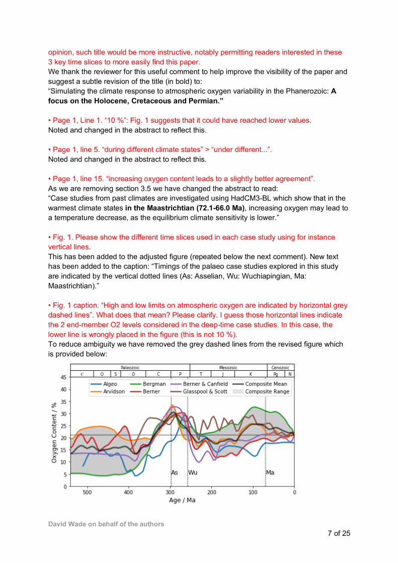
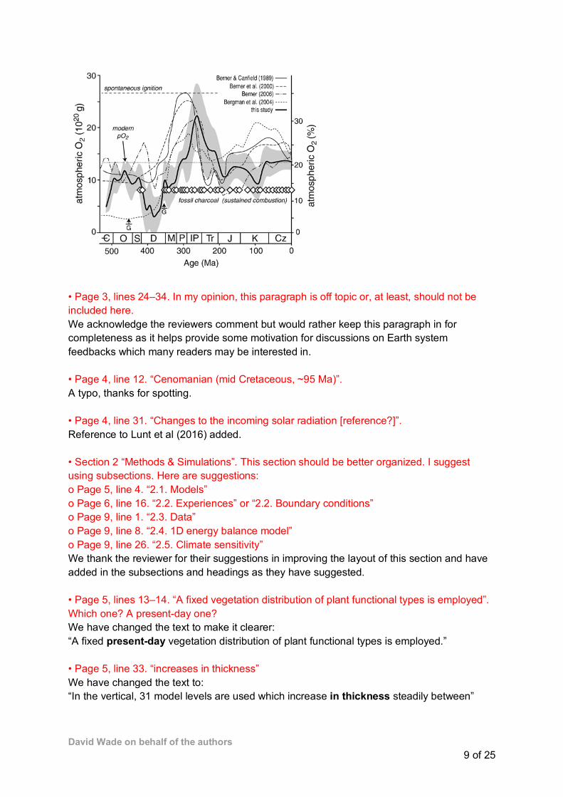
opinion, such title would be more instructive, notably permitting readers interested in these 3 key time slices to more easily find this paper. We thank the reviewer for this useful comment to help improve the visibility of the paper and suggest a subtle revision of the title (in bold) to: “Simulating the climate response to atmospheric oxygen variability in the Phanerozoic: A focus on the Holocene, Cretaceous and Permian.” • Page 1, Line 1. “10 %”: Fig. 1 suggests that it could have reached lower values. Noted and changed in the abstract to reflect this. • Page 1, line 5. “during different climate states” > “under different...”. Noted and changed in the abstract to reflect this. • Page 1, line 15. “increasing oxygen content leads to a slightly better agreement”. As we are removing section 3.5 we have changed the abstract to read: “Case studies from past climates are investigated using HadCM3-BL which show that in the warmest climate states in the Maastrichtian (72.1-66.0 Ma), increasing oxygen may lead to a temperature decrease, as the equilibrium climate sensitivity is lower.” • Fig. 1. Please show the different time slices used in each case study using for instance vertical lines. This has been added to the adjusted figure (repeated below the next comment). New text has been added to the caption: “Timings of the palaeo case studies explored in this study are indicated by the vertical dotted lines (As: Asselian, Wu: Wuchiapingian, Ma: Maastrichtian).” • Fig. 1 caption. “High and low limits on atmospheric oxygen are indicated by horizontal grey dashed lines”. What does that mean? Please clarify. I guess those horizontal lines indicate the 2 end-member O2 levels considered in the deep-time case studies. In this case, the lower line is wrongly placed in the figure (this is not 10 %). To reduce ambiguity we have removed the grey dashed lines from the revised figure which is provided below:


• Page 3, line 1. “to 20–35 % in the Permian and subsequently stabilized at levels around 15–30 % from the Mid Triassic onward” or similar. Thanks for the suggestion which we have adopted directly in the text. • Page 3, line 6. See studies by Dahl et al. (doi:10.1073/pnas.1011287107) and Lu et al. (doi: 10.1126/science.aar5372) though, which provide very interesting insights into the evolution of pO2 during the Phanerozoic. The authors may want to refer to these studies. We’d like to thank the author for bringing these to our attention. We have adapted the sentence in question to “At the time of writing, there are no direct geochemical proxies for atmospheric pO2 on the Phanerozoic timescale. However, there is isotopic evidence of oceanic oxygenation in steps at approximately 560 (Dahl et al 2010), 400 (Dahl et al 2010, Lu et al 2018) and 200 Mya (Lu et al 2018).” • Page 3, line 12. “visible life”. OK, but I’m pretty sure it refers to the ocean realm, not to terrestrial life. Similarly, I think that the most prominent change between the Precambrian and the Phanerozoic is the advent of complex forms of life in the ocean during the Cambrian Explosion and subsequent Ordovician radiation. We don’t mean to diminish the role of the ocean and so suggest modifying the manuscript to read: “visible life and one of the marked.. ”. • Page 3, line 15. “possibly led to the Ordovician glaciation” (there are a lot of alternative hypotheses and the spatial cover and thus climate impact of the primitive Ordovician vegetation remain poorly constrained). We have added “possibly” as the reviewer suggests. • Page 3, lines 17–18. “which is consistent with a long-term sensitivity of the Earth system to CO2”. I do not understand what the authors want to convey here, please rephrase. We have removed this last part of the sentence starting on line 16 page 3. • Page 3, line 21. “continuously since the late Silurian”. Fig. 5 of Algeo and Ingall (doi:10.1016/j.palaeo.2007.02.029) (below) suggests that the charcoal record is more or less continuous since the latest Devonian or so. We thank the reviewer for the comment and have modified the text to reflect the point: “Charcoal appears in the fossil record continuously since the late Devonian (~ 360 Ma, Algeo et al 2007, Scott and Glasspool 2006).”


• Page 3, lines 24–34. In my opinion, this paragraph is off topic or, at least, should not be included here. We acknowledge the reviewers comment but would rather keep this paragraph in for completeness as it helps provide some motivation for discussions on Earth system feedbacks which many readers may be interested in. • Page 4, line 12. “Cenomanian (mid Cretaceous, ~95 Ma)”. A typo, thanks for spotting. • Page 4, line 31. “Changes to the incoming solar radiation [reference?]”. Reference to Lunt et al (2016) added. • Section 2 “Methods & Simulations”. This section should be better organized. I suggest using subsections. Here are suggestions: o Page 5, line 4. “2.1. Models” o Page 6, line 16. “2.2. Experiences” or “2.2. Boundary conditions” o , line 1. “2.3. Data” o Page 9, line 8. “2.4. 1D energy balance model” o Page 9, line 26. “2.5. Climate sensitivity” We thank the reviewer for their suggestions in improving the layout of this section and have added in the subsections and headings as they have suggested. • Page 5, lines 13–14. “A fixed vegetation distribution of plant functional types is employed”. Which one? A present-day one? We have changed the text to make it clearer: “A fixed present-day vegetation distribution of plant functional types is employed.” • Page 5, line 33. “increases in thickness” We have changed the text to: “In the vertical, 31 model levels are used which increase in thickness steadily between”


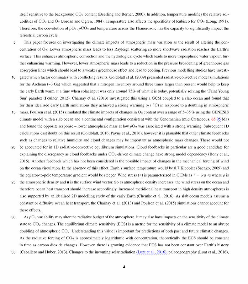
• Fig. 2. Temperature unit? We are not sure what the reviewers comment is? The figures clearly show the surface temperature in degrees Celsius -- the most commonly used unit for the variable -- indicated in both the figure and the figure caption. • Page 6, line 5. “limited to 4 m thick”? Changed. • Page 6, lines 18–19. “as it is possible to alter the model topography and bathymetry”. Please delete. Deleted. • Table 1. o Please explain how the experiments name is built. As it is, the reader has to figure it out himself. The use of “2x” and “4x” in particular, is not obvious. This is placed at the beginning or in the middle of the experiment name and does not refer to any CO2 level but rather seems to multiply the CO2 value used in the baseline runs. Please, explain all this, for instance in the caption of Table 1. Also, what’s the “*”? o What’s the horizontal bar delimiting the 2 parts of Table 1? I guess that “baseline runs” and “sensitivity tests” may be included to refer to each part. The simulation names have been harmonised throughout such that XX-YYY refers to time period XX and model YYY, while a prefix of Nx indicates that the CO2 content has been multiplied by a factor of N with respect to experiment XX-YYY, i.e. 4xPI reads “Four-times preindustrial” which is more intuitive. The horizontal lines now separate the equilibrium experiments from the transient Gregory experiments. The table caption has been expanded to read: “Experiment names AA-BBB include the continental configuration (AA) and model used (BBB). Experiment names NxAA-BBB indicate a multiplier of CO2 with respect to AA-BBB. A star (*) indicates that the CO2 multiplier was applied instantaneously and the transient adjustment to climate was analysed for the purpose of a Gregory 2004 analysis.” o Here and throughout (Table 2, Fig. 6, Fig. 9, Fig. 12, Fig. 16 etc.), I would prefer to see the unit in parentheses rather than with a “/”: “CO2 / Pa” > “CO2 (Pa)”. The use of “/” is confusing when it does not represent a ratio. https://www.bipm.org/en/publications/si-brochure/section5-3.html suggests that SI recommendations are to use “/” to express units so this convention has been retained in the revised manuscript. • Fig. 3. Precipitation unit? + “Continental outline is represented with the thick black line” or similar. We will add “Continental outline is represented with the thick black line.” to both Figure 2 and Figure 3 for consistency. • Page 7, lines 2–4. “The annual average … Figs. 2 and 3.” Please move these lines and figures into the results section.


These are not really results per se, they reflect the standard output of the model for the base simulations and so we argue they belong where they are in the method section as a reference for the reader. • Page 8, line 4. I guess this is “O2 content”. We have changed “O2” to “pO2” to reflect this. • Page 8, line 11. This sounds unlikely, see for instance Fig. 1 of Royer et al. (doi:10.1130/1052-5173(2004)014<4:CAAPDO>2.0.CO;2). We stand by the fact that absolute constraints on pre-quaternary CO2 levels are not as good as those in the quaternary. However, we suggest toning down/rewording the sentence to make it clearer that we mean that the upper limits of CO2 are on the order of ~ 100s of Pa, rather than specifically about 100 Pa. The text now reads: “however there is growing evidence that CO2 is unlikely to have been significantly higher than the order of hundreds of Pa since the radiation of land plants” • Page 9, line 3. “heuristically”. Well, this is obviously “by hand”. Agreed, and as we suggested above this section will be removed. • Page 9, line 24. What’s τs,ebm referring to? The tau was a typo and should be T. We have corrected this in the modified version. • Page 10, line 5. Please define “CS” and “CRE”. They are defined on line 3. • Page 10, lines 14–21. Here and throughout: the text is sometimes difficult to follow because the authors do not refer to figure panels. Please explicitly include “(Fig. 4b)” etc. when appropriate. Also page 13. References to Figure 4a-f have been added at relevant points in the first and second paragraphs of the Surface Climate subsection and references to Figure 6a-f in the final paragraph of the Surface Climate subsection. • Page 10, line 23. “(Figure 4 centre)” > “(Fig. 4 middle column)” Changed • Page 10, lines 25–27. “These could be … reduction with height”. Is this effect really significant? This could be tested with a flat Earth simulation. While the result of this sort of idealised study would be of interest, the intention was to note the possible mechanism rather than to quantify the impacts. • Fig. 4a. Is Panama really open? The plots show the land sea mask employed by the model. In the case of HadGEM3-AO the ocean is not allowed to mix across the isthmus of Panama but the atmosphere component does not resolve the land bridge hence appears open while the ocean is separated. This is a peculiarity of the differing atmosphere and ocean grids employed by the atmosphere and ocean components.


• Fig. 4. Please define the “cold month” and the “warm month”. This has been added as “change in the mean gridbox temperature of the coldest month in the monthly mean climatology” • Table 2. o Missing data for 4xPI-GEM. While preparing the manuscript it became evident that the 4x-PI-GEM21 had not been performed so these results are unfortunatley not available. o The authors may want to include data for their EXP21 experiments in brackets next to their EXP35 results to permit the comparison with Poulsen et al.’s results. We’d like to thank the reviewer for the suggestion and did implement this, however the resulting table was so crowded as to render it unclear so this has not been updated in the revised manuscript. • , line 9. “Comparing the surface temperature (Fig. 4a,b) and precipitation response”. Precipitation is showed in the next paragraph. • Page 12, line 12. “air temperature and precipitation anomalies”. Precipitation is showed in the next paragraph. We’d like to thank the reviewer for noticing these discrepancy. We have moved “Comparing the surface temperature and precipitation response between HadCM3-BL and HadGEM3-AO suggests that the model responses are broadly consistent.” and “A gridbox-by-gridbox comparison of annual mean surface air temperature and precipitation anomalies for PI-GEM35

10 vs PI-CM3510 is presented in Fig. S1. The largest discrepancy in surface air

temperature response between the two models occurs for the largest temperature changes simulated by HadGEM, which is strongest in Northern Hemisphere polar regions. This could be linked to differences in the representation of polar climate processes between the two models. There is broad consistency in cold and warm-month means (Figure 4a and b) with stronger warming in the cold month mean and terrestrial cooling in the warm month mean.” to a new paragraph at the end of the Surface Climate subsection. • Page 12, line 12. “Fig. S1”. Missing supplementary figures? Please check throughout, including on page 15, line 8 + page 18, lines 7–11. We would like to thank the reviewer for drawing this to our attention. We will ensure that the supplementary figures will be submitted with the revised manuscript - based on the reviewers suggestions we will be including many of these in the main text having removed the Model-data comparison and wind stress sections. • Page 13, line 1. “representation of polar climate processes between the two models” + amplification by polar ice feedbacks. The sentence has been adapted to read “This could be linked to differences in the representation of polar climate processes and amplification by polar ice feedbacks between the two models” • Page 13, line 12. Bjerkness compensation. This has been added to the sentence: “A northward shift in the ITCZ would be consistent with stronger warming in the Northern Hemisphere due to Bjerknes compensation (Bjerknes 1964, Broccoli et al. 2006).”


• , line 15. “suggests that pO2 could mediate monsoon climate”. Please check in the model output. Have removed “which suggests that pO2 could mediate monsoon circulations” as there is no supporting analysis. • Fig. 6 caption. “Global mean values (mm/day) are offset”. Please rephrase. As it is, this suggests that values are really offset, which would be annoying. The text label is offset. The global mean values are offset from the plot to the top-right. We have rephrased this from “are offset” to “are offset to the top-right of each plot” as for figure 4. • Fig. 7. and Fig. 8: o Bottom left: What are the dashed lines? o Bottom right: Grey line is missing in the legend. The emissivity is indicated by the dashed purple line and the clearsky emissivity is indicated by the solid purple line while the albedo is indicated by the dashed green line and the clearsky albedo is indicated by the solid green line. The dashed green and dashed purple lines are included again in the bottom-left panel so that the reader can contrast the clear-sky vs all-sky components (the remainder being the cloudy-sky component). We infer from the questions that ambiguity arises from the figure caption, hence this is updated to ensure clarity. The grey line is included in the legend, however is inset in the top-left plot. To ensure that the reader can more easily interpret that the legend entries are common across the plot Figures 7 and 8 have been slightly adjusted: “Bottom left: Clear-sky emissivity (dark purple) and clear-sky albedo (dark green) components of the EBM. The all-sky components are included for comparison. Bottom right: Decomposition of EBM into the total clear-sky (blue), cloudy-sky (red) and all-sky (grey) components.”


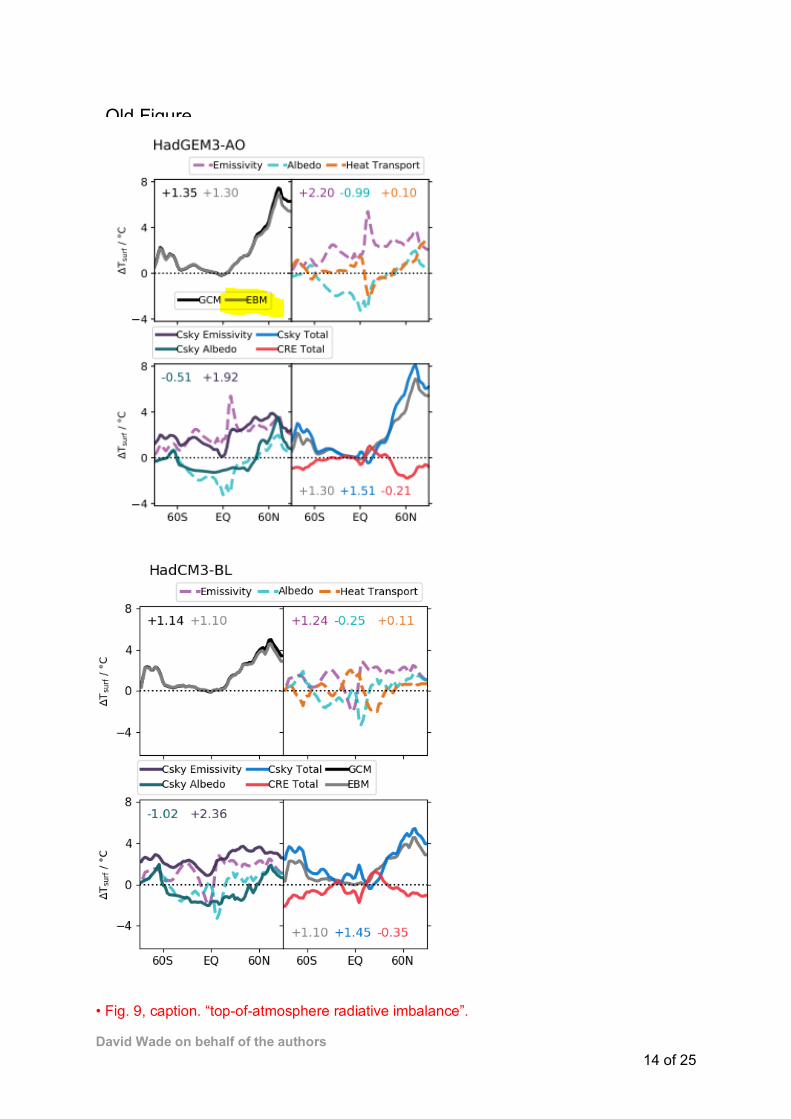
• Fig. 9, caption. “top-of-atmosphere radiative imbalance”.

Old Figure


Thanks - changed “top-of-atmosphere radiative imbalance” • Page 18, line 11. “numerically unstable”. Any idea why? An inspection of the model dump files before the crash revealed very high temperatures in the tropics, however a root cause of the instability could not be found. “Runaway” temperatures* have been found in the MPI model at high CO2 (see Heinmann M., PhD Thesis https://pure.mpg.de/rest/items/item_993927_4/component/file_2388525/content Chapter 3 p40). This limit may have been reached in HadCM3-BL in the context of the Maastrichtian climate. *note this is distinct from a runaway greenhouse effect, the physics of which are typically not properly accounted for in climate models as water vapour is usually assumed to be a minor gas while in a runaway greenhouse will become a major gas and therefore come across similar issues with atmospheric pressure and heat capacity changes. In addition, models would need to better account for water vapour continuum lines than current radiation schemes allow. The rapid runaway temperatures are therefore a model feature rather than an indication that a runaway greenhouse has been reached. • Section 3.4. o I suggest changing the title for something more specific like “Response of Permian vegetation to changing O2 levels” since this section really deals with the Permian case study. At the suggestion of the reviewer we have renamed the section “Response of Permian vegetation to pO2” o The temperature and precipitation dependence of the dominant PFT simulated in the Permian should also be considered. To what extent are the changes in vegetation cover and type due to changes in temperature and precipitation? Changes in precipitation in the Wu-CM runs (Fig. 6e), in particular, seem to spatially correspond to the expansion of the BLT PFT (Fig. 10). I would like to see a short analysis of the environmental affinities of the main PFTs shown on the maps in Fig. 11. I suspect that temperature and precipitation threshold values may play a more important role than changing O2/CO2 ratios. Disentangling the myriad of impacts on vegetation cover would be a challenge. The goal of this section is to highlight that pO2 will have implications beyond those of photorespiration, including the impacts of precipitation and temperature changes. • Fig. 11. The color map is reversed from a to b, which makes it difficult to read. Please revise. The color maps used are different in all three plots as they represent different variables. If the reader has deuteranopia the scales should still be discernible but will appear to be reversed from a to b. • Page 19, line 15. “expansive”. What does than mean? Greater in extent - reworded to “broadleaf trees cover more area in…” • Page 20, line 8. I guess it means that the simulated changes in carbon storage on land do not impact the pCO2 level? It would be good to clearly state what the authors mean by “not interactive”.


This is correct. The sentence now reads “the carbon cycle is not interactive (atmospheric CO2 is fixed)” to clarify this point. • Page 20, lines 20–22. “however, it is likely … equator-to-pole temperature gradient”. Please provide references to support this statement. This section has been removed from the revised manuscript. • Section 3.6 “Importance of Wind Stress”. I get that atmospheric mass impacts wind stress, which in turn impacts the ocean circulation and the heat transport (see page 4, line 20). Unless I get it wrong, those effects are included in the coupled ocean-atmosphere simulations conducted by the authors, which is a good point. However, I do not understand why the authors test the impact of removing wind stress. In my opinion, this section is off topic and should be deleted and possibly kept for another contribution, which would simultaneously shorten the present manuscript and leave the possibility to conduct a robust analysis of the climate response (including the response of ocean dynamics, the analysis of which is essentially lacking so far). (For this reason, I did not include the minor comments relative to this section in this review). We have removed the section, as advised by the review in the major comments above. • Fig. 12, caption. “Proxy data locations (Upchurch et al., 2015) are indicated”. This section has been removed, as advised by the reviewer in the major comments above. • Fig. 14, caption. What’s the unit of precipitation in panel c? Is this an annual mean? The unit mm day-1 has been added to the caption (is already included in the plot). It is annual mean, this has also been added. Now reads: “annual mean precipitation (mm day-1)” NB this is now Figure 15 in the revised paper. • Page 24, line 1. “mainly due to”. We have added the word mainly: “HadCM3-BL simulates a reduced equilibrium climate sensitivity mainly due to changes in longwave cloud feedbacks.” • Page 24, lines 2–3. “The pre-industrial Holocene … of the Archean”. Please support this statement with appropriate references. The references Payne et al (2016), Chemke et al (2016) and Charnay et al (2013) have been added to support the statements made in this sentence. • Page 24, lines 13–15. So, the implementation of pressure broadening is not the same as in Poulsen et al.? Page 7 line 2 suggests that O2 forcing is analogous to Poulsen et al. Please clearly state what’s common between both studies and what’s different. Also, I encourage the authors to make their numerical code available for future work (see major comment). The O2 forcing ought to have been made in an analogous way, however without a deep understanding of the structure of the climate model used and the relevant subcomponents it would not be possible to verify the implementation or identify the commonalities between the implementations. Even if the GENESIS model code and settings were made available, it would be beyond the expertise of the authors to be able to provide a detailed verification. It


is for this reason that we do not believe that releasing model code changes would be useful particularly as the HadCM3-BL and HadGEM3-AO model codebases are under UK crown copyright and the required model changes may vary considerably between models. It is worth noting that while the general approach to changing the pO2 was the same in HadCM3-BL and HadGEM3-AO the specific details are considerably different. Hence we propose that the similarities between the model results and similarities with the more idealised studies elsewhere are what give confidence in the way that the general approach was applied in the specific model versions. • Page 24, lines 18–21. Since sub-daily model output was not written on disk in Wade et al. model runs and thus not made available for analysis, I suggest deleting this comparison that is not that instructive. These two sentences have been removed in the revised manuscript. • Page 24, lines 22–24. Please be cautious: even in a slab model, the continental configuration can impact the ocean heat transport due to the varying ocean area and global climate and thus temperature (which is also impacted by the continental configuration). Another, maybe more robust argument to support the comparison, is that (i) both reconstructions are not so different at first-order and (ii) both simulations provide a relatively close global climate state (compare the mean annual SAT in Poulsen et al. 21% and this study 21% – ca. 18°C vs. 22°C). We thank for reviewer for this suggestion and have included in this sentence, which we have slightly adjusting to clarify which Cretaceous stage was used. “Note that the Poulsen et al. 2015 simulations were for an earlier Cretaceous period (Cenomanian) than those performed in HadCM3-BL (Maastrichtian), however the continental configurations and the global mean temperatures are reasonably similar (22.2 oC in HadCM3-BL vs 20.5 oC in Poulsen et al 2015).” • Page 24, lines 25–31. The contribution of changing ocean dynamics / deep circulation to the simulated climate changes is addressed for the first time here. I suggest either deleting this unsupported statements or providing clear diagnostics of the changes in ocean dynamics. We have removed lines 25-31 and lines 32- p25 l1-2 as both paragraphs discuss the offending material. • Page 25, lines 1–2. The authors may want to refer to Pohl et al. (doi:10.5194/cp-10-2053- 2014), who demonstrated the importance of ocean dynamics to simulate Ordovivician climate changes. We’d like to thank the reviewer for this suggestion. We have removed this paragraph as a result of the above comment, so have not included it in the revised manuscript. • Page 25, lines 5–6. “Increases … high latitudes”. Please provide a reference. Kiehl and Shields 2013 reference has been added. • Page 25, lines 3–14. The authors may also want to refer to the climatic mechanism demonstrated by Rose and Ferreira (doi: 10.1175/JCLI-D-11-00547.1), which was subsequently invoked by Ladant and Donnadieu (doi:10.1038/ncomms12771) to explain the climate changes observed in their Cretaceous model runs.


We’d like to thank the reviewer for this insight, while not completely analogous to Rose and Ferreira the enhanced convection at low pO2 is consistent with an atmospheric moistening. Mechanistically, this is more sensitive in a warmer climate due to Clausius-Clapeyron. The subsequent analysis and addition to the manuscript has been included in a response for AR#3. • Page 25, line 16. “While subsequent experiments have put this in doubt”. Please support this statement with a reference. Wildman et al. 2004 reference added • Page 25, lines 24–25. “although there is evidence of vegetation which causes C4-like fractionation”. During which geological period? Lower Carboniferous - added to the text as “fractionation in the Mississippian, suggesting” • Page 25, line 31. “Other approaches such as trait based methods”. The authors may want to cite Porada et al. (doi: 10.1038/ncomms12113) who applied a trait-based model to simulate the impact of the Ordovician primitive terrestrial vegetation on weathering. We’d like to thank the reviewer for drawing our attention to this interesting and relevant article and have added to the reference in this sentence: “Other approaches such as trait based methods (Van Bodegom et al., 2012; Porada et al., 2016)” • Page 25, line 32 to page 26, line 2. I suggest deleting this paragraph. We have removed “We also have not accounted for changes… may be sensitive to atmospheric pO2 (Clarkson et al., 2018)” inclusive. • Figure 16. The authors previously demonstrated that Poulsen et al.’s implementation of O2 forcing may not be robust. I think this is thus relatively unexpected that they here use those results in their Phanerozoic calculations, even if this may constitute a conservative estimate. I suggest using the results of the current study instead. The motivation for doing so is that even if the climate state was that sensitive to pO2 (which seems unlikely based on previous studies and is also not supported by the proposed study) the differences this causes to global mean temperatures is minor compared to that due to the uncertainty in CO2 content. • Page 27, lines 17–18. “If pCO2 and pO2 … in the Phanerozoic”. Why? Why would cooler climates be associated with higher pO2 levels? I cannot imagine any clear and straightforward explanation to this. CO2 and O2 are linked by photosynthetic productivity and organic carbon burial - increased carbon burial reduces CO2 and increases O2 (CO2 → Corg + O2), see e.g. Montañez 2016 (https://doi.org/10.1073/pnas.1600236113) in the context of pCO2 and pO2 in the Carboniferous-Permian. This mechanism was invoked by Poulsen et al 2015 also. C. Minor points: • Page 3, line 2. “(grey shading in Fig. 1)”. Changed • Page 5, line 13. “which simulates”. Changed


• Page 6, line 12. Reference formatting: “(Valdes et al., 2017)”. Changed • Page 6, lines 20–21. Reference formatting. Changed • Page 7, line 3. Please use correct experiment names instead of 4 x PI-CM21. This has been updated and also now includes the sub-letters as the reviewer kindly suggested in an earlier comment: “Fig. 1 shows the annual average surface temperatures and Fig. 2 shows the annual average precipitation for the (a) PI-CM21, (b) Ma-CM21, (c) Wu-CM21 and (d) As-CM21 simulations.” • Page 8, line 17. “monotically increasing ozone column”. Please rephrase. The ozone column increases monotonically with pO2 in the Harfoot et al 2007 study, hence was described as such in the manuscript. • Page 8, line 29. Reference formatting. Changed • Page 10, line 19. “Wu-CM” (lower-case). Changed • Page 10, line 21. “This suggests that … but is non-linear”. Please revise. We have reworded to “This suggests that the climate response to pO2 variability depends on the background climate state. • Page 12, line 14. “, which are strongest”. Changed • Fig. 5, caption. “4XPI-GEM(red)”: missing space. See also multiple occurrences on page 18, lines 1–5. Changed (fig 5 caption) and updated 5 occurrences page 18. • Fig. 6 color bar labels. Font size issue leading to overlapping text. An adjusted figure has been provided in the revised manuscript • , line 6. “Fig. 11a”. Changed • Page 19, line 16. “reduces” > “reduce” (2 occurrences on the same line). Changed • Page 20, line 13. Please delete question mark. Section removed in the revised manuscript • Page 20, lines 25–26. “These show that across both CO2 contents that increasing”. Please rephrase. Section removed in the revised manuscript • Page 22, lines 4–5. “has the capacity to alter the radiative budget of the atmosphere and therefore on Earth’s climate”. This is verbatim from the original manuscript. Rereading we are suggested to rephrase this text to: “therefore has implications for Earth’s climate.” We hope this aids in the clarity of the sentence. • Page 22, line 6. “with increasing pO2:”. Colon added • Fig. 15, caption. Missing space. Space added • Page 25, line 3. “also contribute”. This sentence has been removed from the revised manuscript.


• Page 25, line 9. “compared”. This sentence has been removed from the revised manuscript. • Page 25, line 13. “which may increase lead to”. Please revise. This sentence has been removed from the revised manuscript. • Page 27, line 7. “PAL”. Please write in full or provide meaning. Changed: PAL → “present atmospheric levels of” • Page 27, line 16. “When pO2 was higher”. Changed: were → was


Anonymous Reviewer #3 The manuscript “Simulating the Climate Response to Atmospheric Oxygen Variability in the Phanerozoic” by Wade et al. presents results from two ocean-atmosphere global circulation models to test the response of temperature, precipitation, and climate sensitivity to variable oxygen levels in earth’s past. The primary results are that increasing oxygen levels causes global temperature to increase, precipitation to decrease, and climate sensitivity to change slightly. These results lead the authors to conclude that oxygen is a secondary factor (to CO2, though presumably also to solar luminosity and paleogeography) in earth’s climate history. The study is mostly very well done, interesting, and well presented. My comments are mostly minor, and should not impede the eventual publication of the manuscript in Climates of the Past. The use of two climate models is a strength of this paper, and I commend the authors for the extra effort. However, without a more in-depth discussion of how the models are different and how the differences lead to the responses reported in the paper, the effort falls a little short. It is worth noting and discussing that both models Edwards and Slingo (1996) radiation scheme. What about other physics schemes? Would other non-Hadley models that don’t share the same physical parameterizations be expected to have larger differences than these two models? While the two models are part of the Met Office Unified Model family of models, the two share few physical schemes except for the use of the Edwards and Slingo radiation scheme, although different versions, and the convection scheme is similar (but with a number of updates between HadCM3-BL and HadGEM3-AO). However, there are a number of large differences. It should be noted that the models do not share the same dynamical core and the cloud and precipitation schemes are different. In addition, the ocean model used is different. Whether other models would be expected to have larger differences will depend on the main driver of those differences. If the radiation scheme would cause the greatest difference, this would not be captured here, for instance. Deconvolving the drivers of differences between the model results to individual physics schemes would require a considerable model development effort and the authors are not aware of any effort to perform such a task in the paleoclimate community. While it is possible to rationalise the differences between models (e.g. Lunt et al 2012 doi:10.5194/cp-8-1717-2012), ascribing these changes to particular model components is much more challenging and beyond the scope of our study. We therefore propose to update the description of model comparison as follows: “, also suggesting this is not a model dependent result. It is worth noting that HadCM3-BL and HadGEM3-AO are not completely distinct climate models, for instance sharing the Edwards and Slingo 1996 radiation scheme, so this is unlikely to capture the full variability in possible climate model responses. That the results are This is in reasonable agreement with the 1-D results of Payne et al. 2016, who simulated a temperature response between +1.05 and +2.21 oC depending on assumptions about atmospheric ozone, gives some confidence in the HadCM3-BL and HadGEM3-AO results. One of the most interesting results in the study is the difference in response with geography,


and specifically the fact that the Wuchiapingian simulations show a temperature response that is opposite of the other runs. This is especially interesting in light of the conflicting results from previous models. The authors need to include an analysis and explanation of this result. The response seen in the Wuchiapingian simulations combined with the lower (less positive) temperature anomaly for 4xPI-GEM35

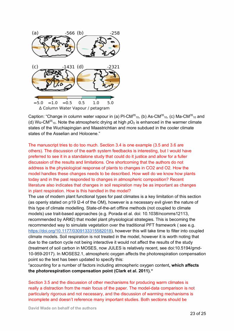
10 motivated the transient CO2 doubling experiments which permit an interrogation of the climate sensitivity and the components that contribute towards these. These are provided in the section Climate Sensitivity and suggest a higher climate sensitivity at low pO2 which is consistent with the order of temperature anomalies across the experiments (higher in cooler climates, smaller to negative for warmer climates). In addition to this, we have investigated a potential cause of the change and propose that the increase in convection at low pO2 increases atmospheric moistening (see figure overleaf) which has a warming effect analogous to Rose and Ferreira 2013. This would serve to explain not only the changes in climate sensitivity but also the temperature response in the Wuchiapingian. Changed around p18 l10: “which tended to cool the low pO2 (Fig. 11). Unlike the clear sky shortwave effects, the longwave cloud radiative effects seem consistent across the three experiments. It should be noted that attempts were made to simulate...” Added final paragraph of Climate Sensitivity subsection: “The increase in climate sensitivity appears to be linked to the reduction in temperature anomaly in a warmer climate state. We propose that this is due to more vigorous convection at low pO2 (Goldblatt et al. 2009) leading to an atmospheric moistening (Fig. 12) which causes warming analogously to Rose and Ferreira 2013. This is consistent with the increases in climate sensitivity observed - in a warmer climate the atmosphere can hold more water vapour, so any changes to water vapour will be amplified in their impacts on the radiative budget of the atmosphere. This water vapour feedback is also consistent with the weaker clear sky shortwave radiative effect observed in 2xMa-CM and the temperature response observed in the Wuchiapingian simulations.”


Caption: “Change in column water vapour in (a) PI-CM35

10, (b) As-CM3510, (c) Ma-CM35

10 and (d) Wu-CM35

10. Note the atmospheric drying at high pO2 is enhanced in the warmer climate states of the Wuchiapingian and Maastrichtian and more subdued in the cooler climate states of the Asselian and Holocene.” The manuscript tries to do too much. Section 3.4 is one example (3.5 and 3.6 are others). The discussion of the earth system feedbacks is interesting, but I would have preferred to see it in a standalone study that could do it justice and allow for a fuller discussion of the results and limitations. One shortcoming that the authors do not address is the physiological response of plants to changes in CO2 and O2. How the model handles these changes needs to be described. How well do we know how plants today and in the past responded to changes in atmospheric composition? Recent literature also indicates that changes in soil respiration may be as important as changes in plant respiration. How is this handled in the model? The use of modern plant functional types for past climates is a key limitation of this section (as openly stated on p19 l2-4 of the OM), however is a necessary evil given the nature of this type of climate modelling. State-of-the-art offline methods (not coupled to climate models) use trait-based approaches (e.g. Porada et al. doi: 10.1038/ncomms12113, recommended by AR#2) that model plant physiological strategies. This is becoming the recommended way to simulate vegetation over the traditional PFT framework ( see e.g. https://doi.org/10.1177/0309133315582018), however this will take time to filter into coupled climate models. Soil respiration is not treated in the model, however it is worth noting that due to the carbon cycle not being interactive it would not affect the results of the study (treatment of soil carbon in MOSES, now JULES is relatively recent, see doi:10.5194/gmd-10-959-2017). In MOSES2.1, atmospheric oxygen affects the photorespiration compensation point so the text has been updated to specify this: “accounting for a number of factors including atmospheric oxygen content, which affects the photorespiration compensation point (Clark et al. 2011).“ Section 3.5 and the discussion of other mechanisms for producing warm climates is really a distraction from the main focus of the paper. The model-data comparison is not particularly rigorous and not necessary, and the discussion of warming mechanisms is incomplete and doesn’t reference many important studies. Both sections should be


deleted. We thank the reviewer for this suggestion and have removed the model-data section from the revised manuscript. We have also removed the paragraph beginning “Increased oxygen content may also contribute to explaining…” Section 3.6 on the influence of wind stress is interesting, but not very insightful without a proper analysis of the explanation for the differences between runs. This section should be removed or (preferably) expanded. How does the total heat transport differ between these runs with and without wind stress? We thank the reviewer for this suggestion and have removed this section from the revised manuscript. One of the main results of the paper is that the response to changes in O2 is very much a function of cloud feedbacks (e.g. Section 3.2). How robust then are the results? How do cloud feedbacks in HadCM and Had GEM3 compare to each other and to other models? This major point is not discussed in the Discussion or presented in the Conclusions. The cloud feedbacks due to pO2 changes have not been assessed in other climate models. Studies of cloud feedbacks in the context of climate models mostly relate to CO2 forcing. The closest analogue to the radiative changes associated with pO2 variability would be solar geoengineering due to the offset of shortwave and longwave radiation. A slightly earlier version of the HadGEM3 model (HadGEM3-ES v6.6.3 vs HadGEM3-AO v7.3) has longwave cloud feedbacks broadly in line with other climate models (Russotto et al. 2018, see https://doi.org/10.5194/acp-18-11905-2018) P. 3, L. 17. “which is consistent with the long-term sensitivity of the Earth system to CO2 changes. . .” I don’t understand this comment. The fact that the CO2 range is constrained should not have an influence on the climate system sensitivity to CO2. We have removed this last part of the sentence starting on line 16 page 3. P. 16, L. 6-7. Please state the climate sensitivity of HadGEM3-AO and HadCM3-BL. This information and references to the values have been added to the text as “For reference, HadGEM3 has a climate sensitivity of +3.6 oC (Nowack et al. 2015) and HadCM3 has a climate sensitivity of +3.1 oC (Johns et al 2006).” P. 18, L. 1. “The clear-sky longwave radiative flux changes are higher in PI2X-CM. . .” That’s not what I see in Fig. 9a. Is there a typo here, or am I misinterpreting something? The change is quite small, so this has been reworded to “radiative flux changes are slightly higher”. P. 18, L. 8. “For Ma-CM, this value is much larger.” This is an interesting result that is not intuitive. The authors should provide a fuller explanation of the large change in sensitivity with this paleogeography and include the figure in the main text. These figures have moved to the main text. The cause of this difference is addressed in the comment above.

Simulating the Climate Response to Atmospheric OxygenVariability in the Phanerozoic

::::::A

:::::::::Focus

:::::on

:::::the

:::::::::::::::Holocene,

::::::::::::::::::Cretaceous

::::::and

:::::::::::::Permian

David C. Wade1, Nathan Luke Abraham1,2, Alexander Farnsworth3, Paul J. Valdes3, Fran Bragg3, andAlexander T. Archibald1,2

1Centre for Atmospheric Science, Department of Chemistry, Cambridge, UK2National Centre for Atmospheric Science, Department of Chemistry, Cambridge, UK3School of Geographical Sciences, University of Bristol, Bristol, UK

Correspondence: [email protected], [email protected]

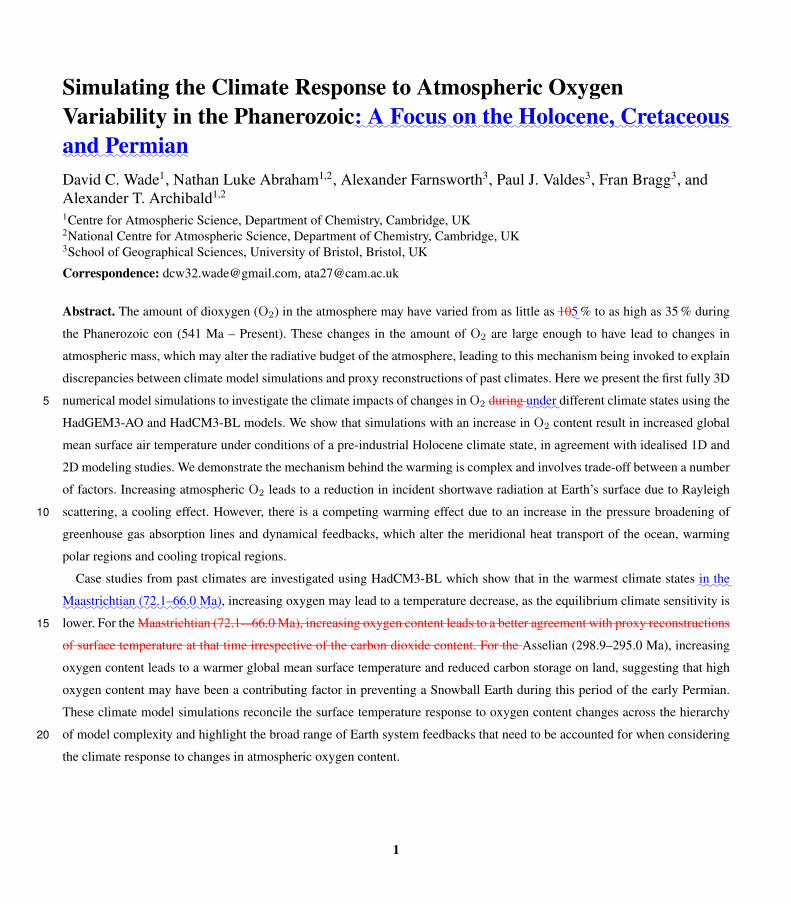
Abstract. The amount of dioxygen (O2) in the atmosphere may have varied from as little as 10:5 % to as high as 35 % during

the Phanerozoic eon (541 Ma – Present). These changes in the amount of O2 are large enough to have lead to changes in

atmospheric mass, which may alter the radiative budget of the atmosphere, leading to this mechanism being invoked to explain

discrepancies between climate model simulations and proxy reconstructions of past climates. Here we present the first fully 3D

numerical model simulations to investigate the climate impacts of changes in O2 during:::::under different climate states using the5

HadGEM3-AO and HadCM3-BL models. We show that simulations with an increase in O2 content result in increased global

mean surface air temperature under conditions of a pre-industrial Holocene climate state, in agreement with idealised 1D and

2D modeling studies. We demonstrate the mechanism behind the warming is complex and involves trade-off between a number

of factors. Increasing atmospheric O2 leads to a reduction in incident shortwave radiation at Earth’s surface due to Rayleigh

scattering, a cooling effect. However, there is a competing warming effect due to an increase in the pressure broadening of10

greenhouse gas absorption lines and dynamical feedbacks, which alter the meridional heat transport of the ocean, warming

polar regions and cooling tropical regions.

Case studies from past climates are investigated using HadCM3-BL which show that in the warmest climate states::in

:::the

:::::::::::Maastrichtian

:::::::::(72.1–66.0

::::Ma), increasing oxygen may lead to a temperature decrease, as the equilibrium climate sensitivity is

lower. For the Maastrichtian (72.1-–66.0 Ma), increasing oxygen content leads to a better agreement with proxy reconstructions15

of surface temperature at that time irrespective of the carbon dioxide content. For the Asselian (298.9–295.0 Ma), increasing

oxygen content leads to a warmer global mean surface temperature and reduced carbon storage on land, suggesting that high

oxygen content may have been a contributing factor in preventing a Snowball Earth during this period of the early Permian.

These climate model simulations reconcile the surface temperature response to oxygen content changes across the hierarchy

of model complexity and highlight the broad range of Earth system feedbacks that need to be accounted for when considering20

the climate response to changes in atmospheric oxygen content.

1

0100200300400500Age / Ma

0

5

10

15

20

25

30

35

40

45

Oxyg

en C

onte

nt /

%

O S D C P T J K Pg NPaleozoic Mesozoic Cenozoic

As Wu Ma

AlgeoArvidson

BergmanBerner

Berner & CanfieldGlasspool & Scott

Composite MeanComposite Range

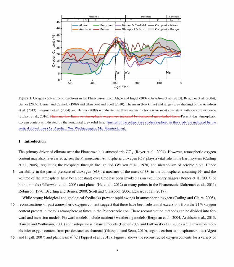
Figure 1. Oxygen content reconstructions in the Phanerozoic from Algeo and Ingall (2007), Arvidson et al. (2013), Bergman et al. (2004),

Berner (2009), Berner and Canfield (1989) and Glasspool and Scott (2010). The mean (black line) and range (grey shading) of the Arvidson

et al. (2013), Bergman et al. (2004) and Berner (2009) is indicated as these reconstructions were most consistent with ice core evidence

(Stolper et al., 2016). High and low limits on atmospheric oxygen are indicated by horizontal grey dashed lines. Present day atmospheric

oxygen content is indicated by the horizontal grey solid line.::::::Timings

::of

::the

::::::palaeo

:::case

::::::studies

::::::explored

::in:::this

:::::study

:::are

:::::::indicated

::by

:::the

:::::vertical

:::::dotted

::::lines

::::(As:

:::::::Asselian,

:::Wu:

::::::::::::Wuchiapingian,

:::Ma:

::::::::::::Maastrichtian).

1 Introduction

The primary driver of climate over the Phanerozoic is atmospheric CO2 (Royer et al., 2004). However, atmospheric oxygen

content may also have varied across the Phanerozoic. Atmospheric dioxygen (O2) plays a vital role in the Earth system (Catling

et al., 2005), regulating the biosphere through fire ignition (Watson et al., 1978) and metabolism of aerobic biota. Hence

variability in the partial pressure of dioxygen (pO2, a measure of the mass of O2 in the atmosphere, assuming N2 and the5

volume of the atmosphere have been constant) over time has been invoked as an evolutionary trigger (Berner et al., 2007) of

both animals (Falkowski et al., 2005) and plants (He et al., 2012) at many points in the Phanerozoic (Saltzman et al., 2011;

Robinson, 1990; Beerling and Berner, 2000; Scott and Glasspool, 2006; Edwards et al., 2017).

While strong biological and geological feedbacks prevent rapid swings in atmospheric oxygen (Catling and Claire, 2005),

reconstructions of past atmospheric oxygen content suggest that there have been substantial excursions from the 21 % oxygen10

content present in today’s atmosphere at times in the Phanerozoic eon. These reconstruction methods can be divided into for-

ward and inversion models. Forward models include nutrient / weathering models (Bergman et al., 2004; Arvidson et al., 2013;

Hansen and Wallmann, 2003) and isotope mass balance models (Berner 2009 and Falkowski et al. 2005) while inversion mod-

els infer oxygen content from proxies such as charcoal (Glasspool and Scott, 2010), organic carbon to phosphorus ratios (Algeo

and Ingall, 2007) and plant resin δ13C (Tappert et al., 2013). Figure 1 shows the reconstructed oxygen contents for a variety of15

2

these methods. There is general agreement in the trends in the reconstructions, in that that oxygen content increased from 5-25%

in the early Paleozoic to 20-35 % in the Permian:::and

:::::::::::subsequently

::::::::stabilised

::at

:::::levels

::::::around

:::::::15-30%

:::::from

:::the

::::Mid

:::::::Triassic

::::::onward. However, there is uncertainty in the absolute amount of O2 for the different reconstructions (grey shading figure

::in

:::Fig.

:1). Indeed, there is support for elevated O2 by carbon isotope measurements

:::::during

::::the

:::::::Permian (Beerling et al., 2002).

However, disagreement is particularly evident in the Mesozoic, with low values simulated by isotope mass balance approaches.5

Mills et al. (2016) have shown that this could be due to an inappropriate choice of δ13C and that adjusting this value with

geological constraints leads to a higher reconstructed oxygen content in better agreement with wildfire records. At the time of

writing, there are no direct geochemical proxies for::::::::::atmospheric

:pO2 on the Phanerozoic timescale. However,

::::there

::is

:::::::isotopic

:::::::evidence

::of

:::::::oceanic

::::::::::oxygenation

::in

:::::steps

::at

::::::::::::approximately

:::560

::::::::::::::::(Dahl et al., 2010),

::::400

::::::::::::::::::::::::::::(Dahl et al., 2010; Lu et al., 2018)

:::and

:::200

::::Mya

::::::::::::::(Lu et al., 2018).

:pO2 in the last 800 000 years has been reconstructed using O2/N2 ratios in ice cores (Stolper et al.,10

2016). A roughly 7‰ decline in pO2 is consistent with the ability to change oxygen content by the order of a few percent in

~ 10 Myr. The reconstructions of Bergman et al. (2004), Arvidson et al. (2013) and Berner (2009) are the most plausible based

on ice core data (Stolper et al., 2016). Considering these three models alone would still suggest a large uncertainty in oxygen

content for most of the Phanerozoic, except for elevated levels in the late Carboniferous / early Permian and reduced levels in

the late Devonian.15

Phanerozoic means ‘visible life’ and the most marked change:::one

::of::::

the::::::marked

:::::::changes

:to carbon cycling between the

Proterozoic and Phanerozoic was caused by the emergence of land plants. The radiation of land plants has led to strong

regulation of atmosphere::::::::::atmospheric

:CO2 and O2 which both play important roles in photosynthesis. Land plants likely

led to a substantial sequestration of carbon in the terrestrial biosphere and::::::possibly

:led to the Ordovician glaciation (Lenton

et al., 2012). Increases in organic carbon sequestration in the aftermath of the evolution of lignin production may also have20

contributed to the cooling (Robinson, 1989). This fundamental change to the Earth system may have constrained CO2 levels

to between 10–200 Pa ever since (Franks et al., 2014)which is consistent with a long-term sensitivity of the Earth system to

changes (Royer, 2016). Watson et al. (1978) have argued that strong fire feedbacks prevent large fluctuations in oxygen levels,

due to runaway burning at high oxygen levels. However subsequent experiments using natural fuels support the possibility of

the Earth system to support higher oxygen levels (Wildman et al., 2004). Charcoal appears in the fossil record continuously25

since the late Silurian (~420::::::::Devonian

:::::(~360 Ma, Scott and Glasspool 2006

::::::::::::::::::::::::::::::::::::::::Algeo and Ingall 2007; Scott and Glasspool 2006

). This suggests a floor on oxygen levels in the region of 12% (Wildman et al., 2004) to 16% (Belcher and McElwain, 2008;

Belcher et al., 2010) since then due to limits on ignition.

Variations in pO2 also have important implications for photosynthesis and therefore the operation of the terrestrial carbon

cycle. The primary CO2-fixing enzyme, Rubisco, possesses a dual carboxylase-oxygenase function (Smith, 1976). A pho-30

tosynthetic carboxylase pathway removes CO2 from the atmosphere while oxygenation leads to photorespiration and CO2

evolution. Therefore, increases in pO2 ought to lead to O2 outcompeting CO2 for active sites on the Rubisco enzyme and lead-

ing to a reduction in net primary productivity (less photosynthesis, more respiration). However, photorespiration is likely to be

necessary for removal of harmful byproducts in the photosynthetic metabolic pathway (Hagemann et al., 2016) and a recent

study suggests that increases in photorespiration may actually promote photosynthesis (Timm et al., 2015). Photosynthesis is35

3

itself sensitive to the background CO2 content (Beerling and Berner, 2000). In addition, temperature modifies the relative sol-

ubilities of CO2 and O2 (Jordan and Ogren, 1984). Temperature also affects the specificity of Rubisco for CO2 (Long, 1991).

Therefore, the coevolution of pO2, pCO2 and temperature across the Phanerozoic has the capacity to significantly impact the

terrestrial carbon cycle.

This paper focuses on investigating the climate impacts of atmospheric mass variation as the result of altering the con-5

centration of O2. Lower atmospheric mass leads to less Rayleigh scattering so more shortwave radiation reaches the Earth’s

surface. This enhances atmospheric convection and the hydrological cycle which leads to more tropospheric water vapour, fur-

ther enhancing warming. However, lower atmospheric mass leads to a reduction in the pressure broadening of greenhouse gas

absorption lines which should lead to a weaker greenhouse effect and lead to cooling. Previous modelling studies have investi-

gated which factor dominates with conflicting results. Goldblatt et al. (2009) presented radiative-convective model simulations10

for the Archean (~3 Ga) which suggested that a nitrogen inventory around three times larger than present would help to keep

the early Earth warm at a time when solar input was only around 75% of what it is today, potentially solving the ‘Faint Young

Sun’ paradox (Feulner, 2012). Charnay et al. (2013) investigated this using a GCM coupled to a slab ocean and found that

for their idealised early Earth simulations they achieved a strong warming (+7 ◦C) in response to a doubling in atmospheric

mass. Poulsen et al. (2015) simulated the climate impacts of changes in O2 content over a range of 5–35 % using the GENESIS15

climate model with a slab ocean and a continental configuration consistent with the Cenomanian (mid Cretaceous, 65::95 Ma)

and found the opposite response – lower atmospheric mass at low pO2 was associated with a strong warming. Subsequent 1D

calculations cast doubt on this result (Goldblatt, 2016; Payne et al., 2016), however it is plausible that other climate feedbacks

such as changes to relative humidity and cloud changes may be important as atmospheric mass changes. These would not

be accounted for in 1D radiative-convective equilibrium simulations. Cloud feedbacks in particular are a good candidate for20

explaining the discrepancy as cloud feedbacks under CO2-driven climate change have strong model dependency (Bony et al.,

2015). Another feedback which has not been considered is the possible impact of changes in the mechanical forcing of wind

on the ocean circulation. In the absence of this effect, Earth’s surface temperature would be 8.7 K cooler (Saenko, 2009) and

the equator-to-pole temperature gradient would be steeper. Wind stress (τ ) is parameterized in GCMs as τ = ρ u ·u where ρ is

the atmospheric density and u is the surface wind vector. So as atmospheric density increases, the wind stress on the ocean and25

therefore ocean heat transport should increase accordingly. Increased meridional heat transport in high density atmospheres is

also supported by an idealised 2D modelling study of the early Earth (Chemke et al., 2016). As slab ocean models assume a

constant or diffusive ocean heat transport, the Charnay et al. (2013) and Poulsen et al. (2015) simulations cannot account for

these effects.

As pO2 variability may alter the radiative budget of the atmosphere, it may also have impacts on the sensitivity of the climate30

state to CO2 changes. The equilibrium climate sensitivity (ECS) is a metric for the sensitivity of a climate model to an abrupt

doubling of atmospheric CO2. Understanding this value is important for predictions of both past and future climatic changes.

As the radiative forcing of CO2 is approximately logarithmic with concentration, theoretically the ECS should be constant

in time as carbon dioxide changes. However, there is growing evidence that ECS has not been constant over Earth’s history

(Caballero and Huber, 2013). Changes to the incoming solar radiation:::::::::::::::(Lunt et al., 2016), palaeogeography (Lunt et al., 2016),35

4

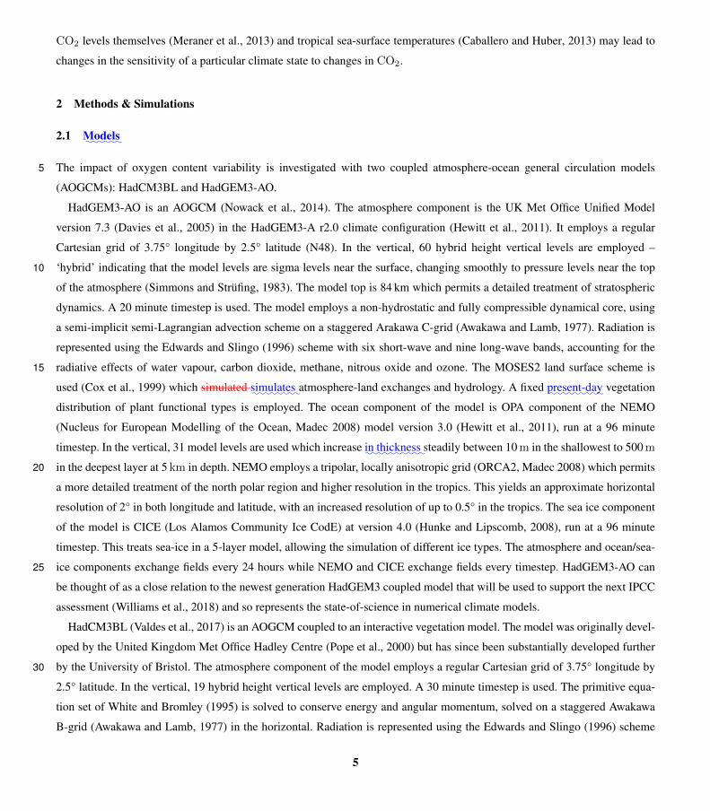
CO2 levels themselves (Meraner et al., 2013) and tropical sea-surface temperatures (Caballero and Huber, 2013) may lead to

changes in the sensitivity of a particular climate state to changes in CO2.

2 Methods & Simulations

2.1::::::

Models

The impact of oxygen content variability is investigated with two coupled atmosphere-ocean general circulation models5

(AOGCMs): HadCM3BL and HadGEM3-AO.

HadGEM3-AO is an AOGCM (Nowack et al., 2014). The atmosphere component is the UK Met Office Unified Model

version 7.3 (Davies et al., 2005) in the HadGEM3-A r2.0 climate configuration (Hewitt et al., 2011). It employs a regular

Cartesian grid of 3.75° longitude by 2.5° latitude (N48). In the vertical, 60 hybrid height vertical levels are employed –

‘hybrid’ indicating that the model levels are sigma levels near the surface, changing smoothly to pressure levels near the top10

of the atmosphere (Simmons and Strüfing, 1983). The model top is 84 km which permits a detailed treatment of stratospheric

dynamics. A 20 minute timestep is used. The model employs a non-hydrostatic and fully compressible dynamical core, using

a semi-implicit semi-Lagrangian advection scheme on a staggered Arakawa C-grid (Awakawa and Lamb, 1977). Radiation is

represented using the Edwards and Slingo (1996) scheme with six short-wave and nine long-wave bands, accounting for the

radiative effects of water vapour, carbon dioxide, methane, nitrous oxide and ozone. The MOSES2 land surface scheme is15

used (Cox et al., 1999) which simulated:::::::simulates

:atmosphere-land exchanges and hydrology. A fixed

:::::::::present-day vegetation

distribution of plant functional types is employed. The ocean component of the model is OPA component of the NEMO

(Nucleus for European Modelling of the Ocean, Madec 2008) model version 3.0 (Hewitt et al., 2011), run at a 96 minute

timestep. In the vertical, 31 model levels are used which increase:in::::::::thickness

:steadily between 10 m in the shallowest to 500 m

in the deepest layer at 5 km in depth. NEMO employs a tripolar, locally anisotropic grid (ORCA2, Madec 2008) which permits20

a more detailed treatment of the north polar region and higher resolution in the tropics. This yields an approximate horizontal

resolution of 2° in both longitude and latitude, with an increased resolution of up to 0.5° in the tropics. The sea ice component

of the model is CICE (Los Alamos Community Ice CodE) at version 4.0 (Hunke and Lipscomb, 2008), run at a 96 minute

timestep. This treats sea-ice in a 5-layer model, allowing the simulation of different ice types. The atmosphere and ocean/sea-

ice components exchange fields every 24 hours while NEMO and CICE exchange fields every timestep. HadGEM3-AO can25

be thought of as a close relation to the newest generation HadGEM3 coupled model that will be used to support the next IPCC

assessment (Williams et al., 2018) and so represents the state-of-science in numerical climate models.

HadCM3BL (Valdes et al., 2017) is an AOGCM coupled to an interactive vegetation model. The model was originally devel-

oped by the United Kingdom Met Office Hadley Centre (Pope et al., 2000) but has since been substantially developed further

by the University of Bristol. The atmosphere component of the model employs a regular Cartesian grid of 3.75° longitude by30

2.5° latitude. In the vertical, 19 hybrid height vertical levels are employed. A 30 minute timestep is used. The primitive equa-

tion set of White and Bromley (1995) is solved to conserve energy and angular momentum, solved on a staggered Awakawa

B-grid (Awakawa and Lamb, 1977) in the horizontal. Radiation is represented using the Edwards and Slingo (1996) scheme

5

(a) 14.4 (b) 22.2

(c) 23.9 (d) 14.5

40 30 20 10 0 10 20 30 40Surface Air Temperature / °C

Figure 2. Annual average surface air temperature simulated in (a) PI-CM21, (b) Ma-CM21, (c) Wu-CM21 and (d) As-CM21. Global mean

values are inset top right. The 0 Celsius isoline is indicated in pink.::::::::Continental

::::::outlines

:::are

:::::::indicated

::::with

:a::::solid

::::black

::::line.

with six short-wave and eight long-wave bands, accounting for the radiative effects of water vapour, carbon dioxide and ozone,

amongst other radiative active species. The ocean component of the model employs the same horizontal grid as the atmo-

sphere component of the model, 3.75° longitude by 2.5° latitude. In the vertical, 20 model levels are used which increase in

depth from 10 m in the shallowest layer to 616 m in the deepest layer. A timestep of 60 minutes is employed and the ocean

and atmosphere components exchange required fields once per day. The ocean component is based on the Cox (1984) model,5

solving the full primitive equation set in three-dimensions. A staggered Awakawa B-grid is employed in both atmosphere and

ocean models. Sea-ice is treated as a zero thickness layer on the surface of the ocean grid. Ice is assumed to form at the base

at a freezing point of –1.8 ◦C but can also form from freezing in ice leads and by falling snow. A simple parameterisation of

sea-ice dynamics is also employed (Gordon et al., 2000) and sea-ice formation due to convergence from drift is limited to 4 m

deep::::thick. Sea-ice albedo is fixed at 0.8 for temperatures below –10 ◦C, decreasing linearly to 0.5 at 0 ◦C. The MOSES2.1 land10

surface model is employed to simulate the fluxes of energy and water between the land surface and the atmosphere (Cox et al.,

2000; Essery et al., 2003). TRIFFID (Top-down Representation of Interactive Foliage and Flora Including Dynamics, Cox

et al. 1998) predicts the distribution of vegetation using a plant functional type (PFT) approach. TRIFFID is run in equilibrium

mode with averaged fluxes calculated over a 5 year period. TRIFFID calculates vegetation properties for five PFTs: broadleaf

trees, needleleaf tree, C3 grass, C4 grass and shrubs. Gridboxes can contain a mixture of PFTs based on a ‘fractional cover-15

age co-existence approach’ Valdes et al. (2017)::::::::::::::::(Valdes et al., 2017). Net primary productivity (NPP) is also calculated, using a

photosynthesis-stomatal conductance model (Cox et al., 1998) accounting for a number of factors including atmospheric oxy-

gen content:,:::::which

::::::affects

:::the

::::::::::::::photorespiration

::::::::::::compensation

::::point

::::::::::::::::(Clark et al., 2011). The predicted vegetation distribution

impacts the atmosphere component by altering surface albedo, evapotranspiration and surface roughness. Simulations have

been run for 1422 model years reaching an equilibration state at the surface.20

6

(a) 2.92 (b) 3.28

(c) 3.27 (d) 2.88

0 1 3 5 7 9Total Precipitation / mm day 1

Figure 3. Annual average precipitation simulated in (a) PI-CM21, (b) Ma-CM21, (c) Wu-CM21 and (d) As-CM21. Global mean values are

inset top right.::::::::Continental

::::::outlines

:::are

:::::::indicated

::::with

:a::::solid

::::black

::::line.

2.2::::::::Boundary

::::::::::Conditions

Both models simulated the climate response to oxygen variability in a preindustrial Holocene (PIH) climate. HadCM3-BL was

additionally run for three time periods across the Phanerozoic: The Maastrichtian (late Cretaceous, 66.0–72.1 Ma), Wuchiapin-

gian (late Permian, 254.14–259.1 Ma) and the Asselian (early Permian, 295.0–298.9 Ma)as it is possible to alter the model

topography and bathymetry. The continental reconstructions employed were developed by and are ©Getech. These reconstruc-5

tions have been widely employed in a number of previous studies using the HadCM3-BL climate model (e.g. (Lunt et al., 2016)

:::::::::::::Lunt et al. 2016). All three are periods of time in which models have suggested that atmospheric oxygen may have deviated

significantly from the present level of 21 % (see Fig. 1). Modifications were made to alter the oxygen content of the atmosphere

by adjusting the mass mixing ratios of major and minor gases, the surface pressure and other physical characteristics of the

atmosphere such as the specific gas constant in an analogous way to Poulsen et al. (2015). The::::Fig.

:2:::::shows

:::the

:annual average10

surface temperatures and:::Fig.

::3

:::::shows

:::the

:annual average precipitation for

::the

:::(a)

:PI-CM21, PI-CM

::(b)

:::::::Ma-CM21, PI-CM

::(c)

:::::::Wu-CM21 and PI-CM

::(d)

:::::::As-CM21 simulationsare shown in Figs. 2 and 3. .

:

A summary of the experiments performed can be found in Table 1. When an experiment with a particular oxygen content

is referred to, it will be indicated in superscript, e.g. EXP21 indicates a 21 % oxygen simulation. 21 % simulations (PI-CM21,

As-CM21, Ma-CM21 and Wu-CM21) were integrated for 50 model years as these simulations had already been spun up at that15

CO2 content. For 10 % and 35 %:pO2 the model was spun off the 21 %

:pO2 simulation and iterated for at least 1000 model

years. The PI2x-CM*, Ma2x-CM* and As2x-CM*:::::::::2xPI-CM*,

::::::::::2xMa-CM*

:::and

::::::::::2xAs-CM*

:experiments were spun off from

the end of the PI-CM, Ma-CM and As-CM experiments and iterated for 100 , 1000 and 100 years respectively::::years

::in

:::::order

::to

::::::perform

::a::::::::::::::::::Gregory et al. (2004)

::::::analysis. For HadGEM3-AO, model integrations (PI-GEM35, PI-GEM10, 4xPI-GEM35 and

4xPI-GEM10) were performed for 300 model years with a 10-times acceleration of the deep ocean to reduce the time for20

7

Table 1. Summary of experiments.:::::::::Experiment

:::::names

::::::::AA-BBB

::::::include

:::the

:::::::::continental

::::::::::configuration

:::::(AA)

:::and

::::::model

::::used

::::::(BBB).

::::::::Experiment

::::::names

:::::::::NxAA-BBB

:::::::indicate

:a::::::::multiplier

::of CO2 :::

with::::::respect

::to

:::::::AA-BBB.

::A::::

star::(*)

:::::::indicates

::::that

::the

:CO2 :::::::

multiplier::::

was

:::::applied

::::::::::::instantaneously

:::and

:::the

::::::transient

:::::::::adjustment

:to::::::

climate:::was

:::::::analysed

:::for

::the

:::::::purpose

::of

:a::::::::::::::::Gregory et al. (2004)

::::::analysis.

Experiment Continents Model CO2 / Pa O2 / % Notes

PI-GEM PIH HadGEM3-AO 28 10,21,35

4xPI-GEM PIH HadGEM3-AO 112 10,35

PI-CM PIH HadCM3-BL 28 10,21,35

Ma-CM Maastrichtian HadCM3-BL 56 10,21,35

As-CM Asselian HadCM3-BL 28 10,21,35

Wu-CM Wuchiapingian HadCM3-BL 112 10,21,35

τPI-CM*:::::::2xPI-CM*

:PIH HadCM3-BL 28 21 1 τMa-CM* Maastrichtian HadCM3-BL 56 21 1 τAs-CM* Asselian HadCM3-BL 28 21 1 τWu-CM* Wuchiapingian HadCM3-BL 112 21 1 PI2x-CM* PIH HadCM3-BL 56 10,21,35

Ma2x-CM*:::::::::2xMa-CM* Maastrichtian HadCM3-BL 112 10,21,35

As2x-CM*::::::::2xAs-CM* Asselian HadCM3-BL 56 10,21,35

equilibrium then integrated for a further 500 years to spin up the shallow ocean without acceleration. The last 50 years were

used for model analysis.

Pre-Quaternary pCO2 is poorly constrained due to the absence of glacial ice, however there is growing evidence that CO2

is unlikely to have been significantly higher than ~100::the

:::::order

::of

::::::::hundreds

::of

:Pa since the radiation of land plants (Breecker

et al., 2010; Franks et al., 2014). For the Maastrichtian, 56 Pa is used in agreement with stomatal proxy-based reconstructions5

(Steinthorsdottir and Pole, 2016). For the Asselian, 28 Pa is used in agreement with carbonate and fossil plant reconstructions

(Montañez et al., 2007). For the Wuchiapingian, 112 Pa is used (Brand et al., 2012).

1D atmospheric chemistry simulations have simulated higher O3 column with increasing pO2 (Kasting et al., 1979; Payne

et al., 2016). More detailed 2D model simulations, which capture critical latitudinal gradients in photolysis and zonal mean

transport (Hadjinicolaou and Pyle, 2004; Haigh and Pyle, 1982), support a monotonically increasing ozone column with in-10

creasing pO2 (Harfoot et al., 2007). However, simulated ozone column was more sensitive to N2O levels than pO2 (Harfoot

et al., 2007). In addition, while column ozone reduces at low pO2 in Harfoot et al. (2007) there are increases in ozone con-

centration in the tropical tropopause region where the radiative effect of O3 is stronger (Forster and Shine, 1997). Changes in

lightning are important for understanding future changes in tropospheric ozone (Banerjee et al., 2014), however are subject

to considerable uncertainty (Finney et al., 2018). There may be more lightning at high pO2 due to a higher pO2/pN2 ratio15

or less due to reduced convection (Goldblatt et al., 2009). Low pO2 may also enhance isoprene emissions (Rasulov et al.,

2009), which could enhance tropospheric ozone and alter cloud properties (Kiehl and Shields, 2013). Ozone is also sensitive to

changes in CH4 and N2O, the changes to inventories of these chemically-active species on the Phanerozoic timescale (Beer-

ling et al., 2009, 2011) is highly uncertain. Ozone is also sensitive to dynamical changes. Given these large uncertainties in

possible changes to chemical sources, reactivity and transport we neglected including changes in atmospheric ozone concen-20

8

tration in these simulations. However, we recommend that follow up work should focus on this specific question in detail. In

HadGEM3-AO the mass of tropospheric and stratospheric ozone is fixed at PIH values simulated by (Nowack et al., 2014)

:::::::::::::::::Nowack et al. (2014) using a tropopause height matching scheme. This prevents a rising tropopause leading to stratospheric

levels of ozone existing in the troposphere, particularly in the 4xPI-GEM experiments. Not accounting for a rising tropopause

has been found to artificially increase climate sensitivity (Heinemann, 2009) and initial tests not accounting for this led to5

instability for 4xPI-GEM10. In HadCM3-BL, tropospheric ozone is set to 6 ppbv and stratospheric ozone is set to 1.66 ppmv

for the 21 % simulations. These values are adjusted to conserve total ozone mass in the alternative pO2 scenarios.

Proxy data for the Maastrichtian was obtained from Upchurch et al. (2015) and interpolated from their modern locations

on to the ©Getech grid. Where the proxy locations deviated substantially from those described in Upchurch et al. (2015)

(i.e. terrestrial proxy in the ocean) these were adjusted heuristically. The proxy data was obtained by a variety of methods10

including TEX86, δ18O and leaf margin analysis. A full description of the proxy data and methods used can be found in

Upchurch et al. (2015) and reference therein.

2.3::::

Data

Data for the Cenomanian Poulsen et al. (2015) 21 % O2 and 10 % O2 simulations were obtained from https://www.ncdc.noaa.

gov/paleo/study/18776. At the time of writing the 35 % simulation contained missing data so was not used for analysis.15

2.4::1D

:::::::Energy

:::::::Balance

::::::Model

A 1D energy balance model (EBM) has been used to deconvolve the contributions from changes in different parts of the

climate system. This 1D-EBM approach has been applied to zonal mean quantities for climate simulations of the Eocene by

Heinemann et al. (2009) following Budyko (1969) and Sellers (1969):

SW↓t (φ)[1−α(φ)]− 1

2πR2cos(φ)

∂F (φ)

∂φ= ε(φ)σT 4

s,ebm(φ) (1)20

where SW↓t is the incident shortwave radiation at the top-of-the atmosphere, φ is the latitude, α is the surface albedo, R is the

radius of Earth, ε is the effective surface emissivity and Ts,ebm is the EBM surface temperature (Heinemann et al., 2009). ∂F (φ)∂φ

is the divergence of total meridional heat transport and is given by

∂F (φ)

∂φ= −2πR2cos(φ)(SWnet

t (φ) + LWnett (φ)) (2)

where SWnett and LWnet

t are the net top-of-atmosphere shortwave and longwave radiative fluxes respectively (positive down-25

ward, Heinemann et al. 2009). Solving for Ts,ebm, the EBM surface temperature for each latitude can be calculated using zonal

and annual mean radiative fluxes from the GCM. Where clear-sky radiative fluxes are also available, cloud radiative effects can

be deconvolved from clear-sky radiative effects. The clear-sky albedo αc and clear-sky effective surface emissivity εc can be

calculated by:

αc =SW↑t,cSW↓t

, εc =LW↑t,cLW↑s

(3)30

9

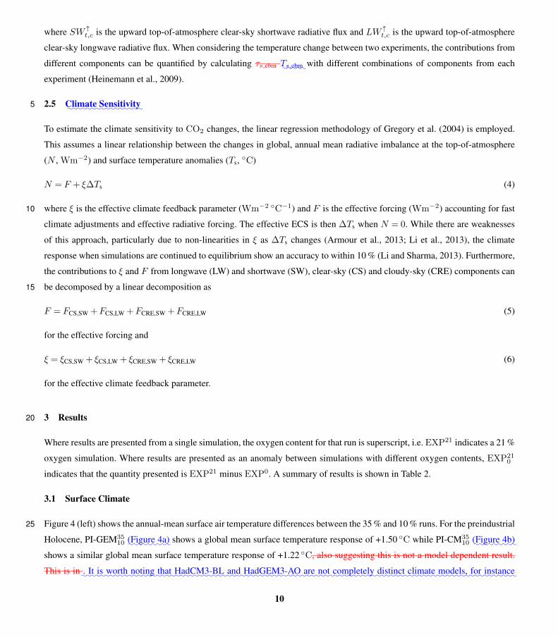
where SW ↑t,c is the upward top-of-atmosphere clear-sky shortwave radiative flux and LW ↑t,c is the upward top-of-atmosphere

clear-sky longwave radiative flux. When considering the temperature change between two experiments, the contributions from

different components can be quantified by calculating τs,ebm ::::Ts,ebm:with different combinations of components from each

experiment (Heinemann et al., 2009).

2.5::::::

Climate::::::::::Sensitivity5

To estimate the climate sensitivity to CO2 changes, the linear regression methodology of Gregory et al. (2004) is employed.

This assumes a linear relationship between the changes in global, annual mean radiative imbalance at the top-of-atmosphere

(N , Wm−2) and surface temperature anomalies (Ts, ◦C)

N = F + ξ∆Ts (4)

where ξ is the effective climate feedback parameter (Wm−2 ◦C−1) and F is the effective forcing (Wm−2) accounting for fast10

climate adjustments and effective radiative forcing. The effective ECS is then ∆Ts when N = 0. While there are weaknesses

of this approach, particularly due to non-linearities in ξ as ∆Ts changes (Armour et al., 2013; Li et al., 2013), the climate

response when simulations are continued to equilibrium show an accuracy to within 10 % (Li and Sharma, 2013). Furthermore,

the contributions to ξ and F from longwave (LW) and shortwave (SW), clear-sky (CS) and cloudy-sky (CRE) components can

be decomposed by a linear decomposition as15

F = FCS,SW +FCS,LW +FCRE,SW +FCRE,LW (5)

for the effective forcing and

ξ = ξCS,SW + ξCS,LW + ξCRE,SW + ξCRE,LW (6)

for the effective climate feedback parameter.

3 Results20

Where results are presented from a single simulation, the oxygen content for that run is superscript, i.e. EXP21 indicates a 21 %

oxygen simulation. Where results are presented as an anomaly between simulations with different oxygen contents, EXP210

indicates that the quantity presented is EXP21 minus EXP0. A summary of results is shown in Table 2.

3.1 Surface Climate

Figure 4 (left) shows the annual-mean surface air temperature differences between the 35 % and 10 % runs. For the preindustrial25

Holocene, PI-GEM3510 ::::::

(Figure:::4a) shows a global mean surface temperature response of +1.50 ◦C while PI-CM35

10 ::::::(Figure

:::4b)

shows a similar global mean surface temperature response of +1.22 ◦C, also suggesting this is not a model dependent result.

This is in:.::It

::is

:::::worth

::::::noting

:::that

::::::::::::HadCM3-BL

:::and

:::::::::::::HadGEM3-AO

:::are

:::not

::::::::::completely

::::::distinct

:::::::climate

:::::::models,

:::for

:::::::instance

10

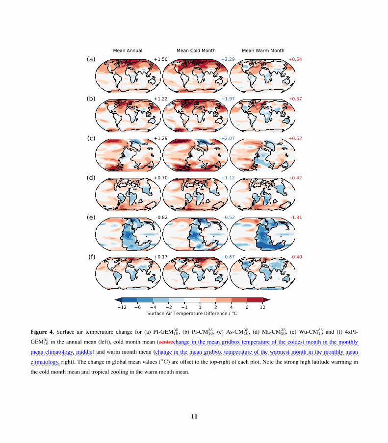
(a) +1.50 +2.29 +0.64

(b) +1.22 +1.97 +0.57

(c) +1.29 +2.07 +0.62

(d) +0.70 +1.12 +0.42

(e) -0.82 -0.52 -1.31

(f) +0.17 +0.67 -0.40

12 6 4 2 1 1 2 4 6 12Surface Air Temperature Difference / °C

Mean Annual Mean Cold Month Mean Warm Month

Figure 4. Surface air temperature change for (a) PI-GEM3510, (b) PI-CM35

10, (c) As-CM3510, (d) Ma-CM35

10, (e) Wu-CM3510 and (f) 4xPI-

GEM3510 in the annual mean (left), cold month mean (centre

:::::change

::in

:::the

::::mean

::::::gridbox

::::::::::temperature

::of

::the

::::::coldest

:::::month

::in:::

the:::::::monthly

::::mean

:::::::::climatology,

::::::middle) and warm month mean (

:::::change

::in:::

the:::::mean

::::::gridbox

:::::::::temperature

::of

:::the

:::::::warmest

:::::month

::in

:::the

::::::monthly

:::::mean

:::::::::climatology, right). The change in global mean values (◦C) are offset to the top-right of each plot. Note the strong high latitude warming in

the cold month mean and tropical cooling in the warm month mean.

11

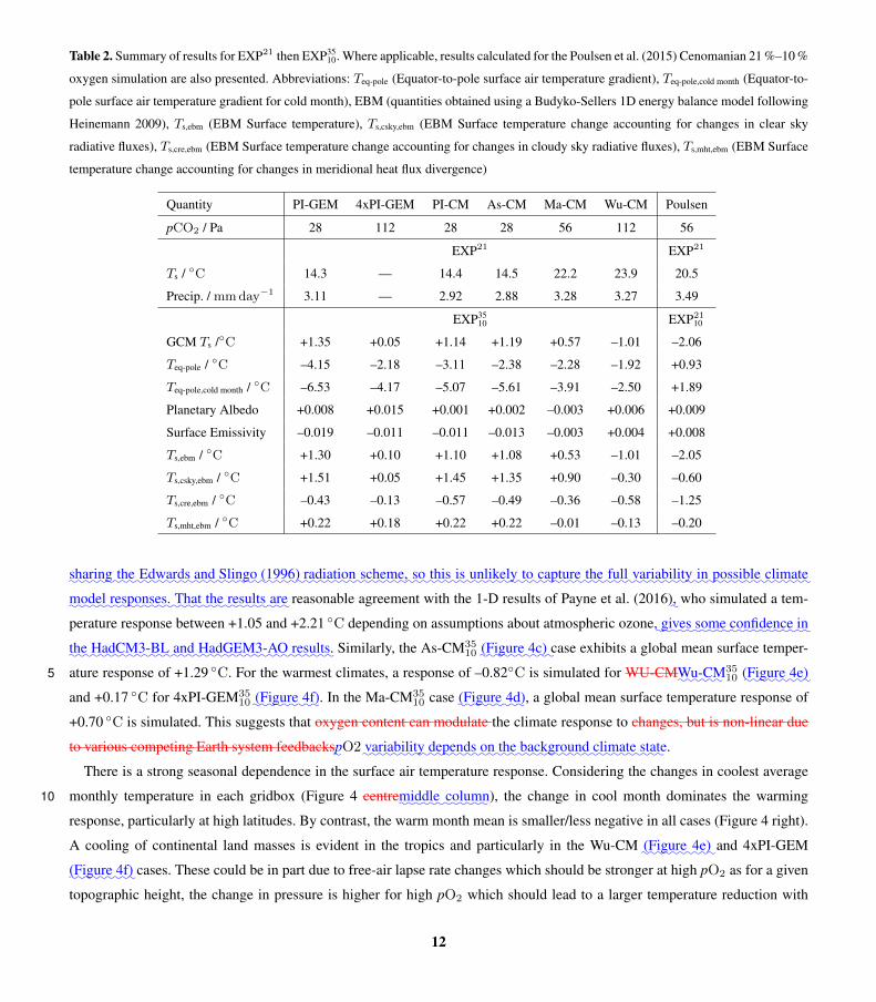
Table 2. Summary of results for EXP21 then EXP3510. Where applicable, results calculated for the Poulsen et al. (2015) Cenomanian 21 %–10 %

oxygen simulation are also presented. Abbreviations: Teq-pole (Equator-to-pole surface air temperature gradient), Teq-pole,cold month (Equator-to-

pole surface air temperature gradient for cold month), EBM (quantities obtained using a Budyko-Sellers 1D energy balance model following

Heinemann 2009), Ts,ebm (EBM Surface temperature), Ts,csky,ebm (EBM Surface temperature change accounting for changes in clear sky

radiative fluxes), Ts,cre,ebm (EBM Surface temperature change accounting for changes in cloudy sky radiative fluxes), Ts,mht,ebm (EBM Surface

temperature change accounting for changes in meridional heat flux divergence)

Quantity PI-GEM 4xPI-GEM PI-CM As-CM Ma-CM Wu-CM Poulsen

pCO2 / Pa 28 112 28 28 56 112 56

EXP21 EXP21

Ts / ◦C 14.3 — 14.4 14.5 22.2 23.9 20.5

Precip. / mmday−1 3.11 — 2.92 2.88 3.28 3.27 3.49

EXP3510 EXP21

10

GCM Ts /◦C +1.35 +0.05 +1.14 +1.19 +0.57 –1.01 –2.06

Teq-pole / ◦C –4.15 –2.18 –3.11 –2.38 –2.28 –1.92 +0.93

Teq-pole,cold month / ◦C –6.53 –4.17 –5.07 –5.61 –3.91 –2.50 +1.89

Planetary Albedo +0.008 +0.015 +0.001 +0.002 –0.003 +0.006 +0.009

Surface Emissivity –0.019 –0.011 –0.011 –0.013 –0.003 +0.004 +0.008

Ts,ebm / ◦C +1.30 +0.10 +1.10 +1.08 +0.53 –1.01 –2.05

Ts,csky,ebm / ◦C +1.51 +0.05 +1.45 +1.35 +0.90 –0.30 –0.60

Ts,cre,ebm / ◦C –0.43 –0.13 –0.57 –0.49 –0.36 –0.58 –1.25

Ts,mht,ebm / ◦C +0.22 +0.18 +0.22 +0.22 –0.01 –0.13 –0.20

::::::sharing

:::the

:::::::::::::::::::::::Edwards and Slingo (1996)

:::::::radiation

:::::::scheme,

:::so

:::this

::is

:::::::unlikely

::to

:::::::capture

:::the

:::full

:::::::::variability

::in

:::::::possible

:::::::climate

:::::model

:::::::::responses.

::::That

:::the

::::::results

:::are reasonable agreement with the 1-D results of Payne et al. (2016)

:, who simulated a tem-

perature response between +1.05 and +2.21 ◦C depending on assumptions about atmospheric ozone,:::::gives

:::::some

:::::::::confidence

::in

::the

::::::::::::HadCM3-BL

:::and

:::::::::::::HadGEM3-AO

::::::results. Similarly, the As-CM35

10 ::::::(Figure

:::4c)

:case exhibits a global mean surface temper-

ature response of +1.29 ◦C. For the warmest climates, a response of –0.82◦C is simulated for WU-CM::::::Wu-CM35

10 ::::::(Figure

:::4e)5

and +0.17 ◦C for 4xPI-GEM3510 ::::::

(Figure:::4f). In the Ma-CM35

10 case::::::(Figure

:::4d), a global mean surface temperature response of

+0.70 ◦C is simulated. This suggests that oxygen content can modulate the climate response to changes, but is non-linear due

to various competing Earth system feedbacks:pO2

::::::::variability

::::::::depends

::on

:::the

::::::::::background

::::::climate

::::state.

There is a strong seasonal dependence in the surface air temperature response. Considering the changes in coolest average

monthly temperature in each gridbox (Figure 4 centre:::::middle

:::::::column), the change in cool month dominates the warming10

response, particularly at high latitudes. By contrast, the warm month mean is smaller/less negative in all cases (Figure 4 right).

A cooling of continental land masses is evident in the tropics and particularly in the Wu-CM::::::(Figure

:::4e)

:and 4xPI-GEM

::::::(Figure

:::4f) cases. These could be in part due to free-air lapse rate changes which should be stronger at high pO2 as for a given

topographic height, the change in pressure is higher for high pO2 which should lead to a larger temperature reduction with

12

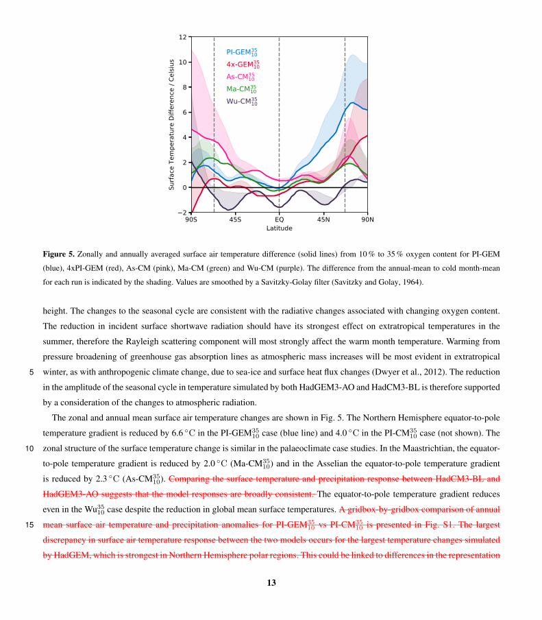
90S 45S EQ 45N 90NLatitude

2

0

2

4

6

8

10

12

Surfa

ce T

empe

ratu

re D

iffer

ence

/ Ce

lsius

PI-GEM3510

4x-GEM3510

As-CM3510

Ma-CM3510

Wu-CM3510

Figure 5. Zonally and annually averaged surface air temperature difference (solid lines) from 10 % to 35 % oxygen content for PI-GEM

(blue), 4xPI-GEM (red), As-CM (pink), Ma-CM (green) and Wu-CM (purple). The difference from the annual-mean to cold month-mean

for each run is indicated by the shading. Values are smoothed by a Savitzky-Golay filter (Savitzky and Golay, 1964).

height. The changes to the seasonal cycle are consistent with the radiative changes associated with changing oxygen content.

The reduction in incident surface shortwave radiation should have its strongest effect on extratropical temperatures in the

summer, therefore the Rayleigh scattering component will most strongly affect the warm month temperature. Warming from

pressure broadening of greenhouse gas absorption lines as atmospheric mass increases will be most evident in extratropical

winter, as with anthropogenic climate change, due to sea-ice and surface heat flux changes (Dwyer et al., 2012). The reduction5

in the amplitude of the seasonal cycle in temperature simulated by both HadGEM3-AO and HadCM3-BL is therefore supported

by a consideration of the changes to atmospheric radiation.

The zonal and annual mean surface air temperature changes are shown in Fig. 5. The Northern Hemisphere equator-to-pole

temperature gradient is reduced by 6.6 ◦C in the PI-GEM3510 case (blue line) and 4.0 ◦C in the PI-CM35

10 case (not shown). The

zonal structure of the surface temperature change is similar in the palaeoclimate case studies. In the Maastrichtian, the equator-10

to-pole temperature gradient is reduced by 2.0 ◦C (Ma-CM3510) and in the Asselian the equator-to-pole temperature gradient

is reduced by 2.3 ◦C (As-CM3510). Comparing the surface temperature and precipitation response between HadCM3-BL and

HadGEM3-AO suggests that the model responses are broadly consistent. The equator-to-pole temperature gradient reduces

even in the Wu3510 case despite the reduction in global mean surface temperatures. A gridbox-by-gridbox comparison of annual

mean surface air temperature and precipitation anomalies for PI-GEM3510 vs PI-CM35

10 is presented in Fig. S1. The largest15

discrepancy in surface air temperature response between the two models occurs for the largest temperature changes simulated

by HadGEM, which is strongest in Northern Hemisphere polar regions. This could be linked to differences in the representation

13

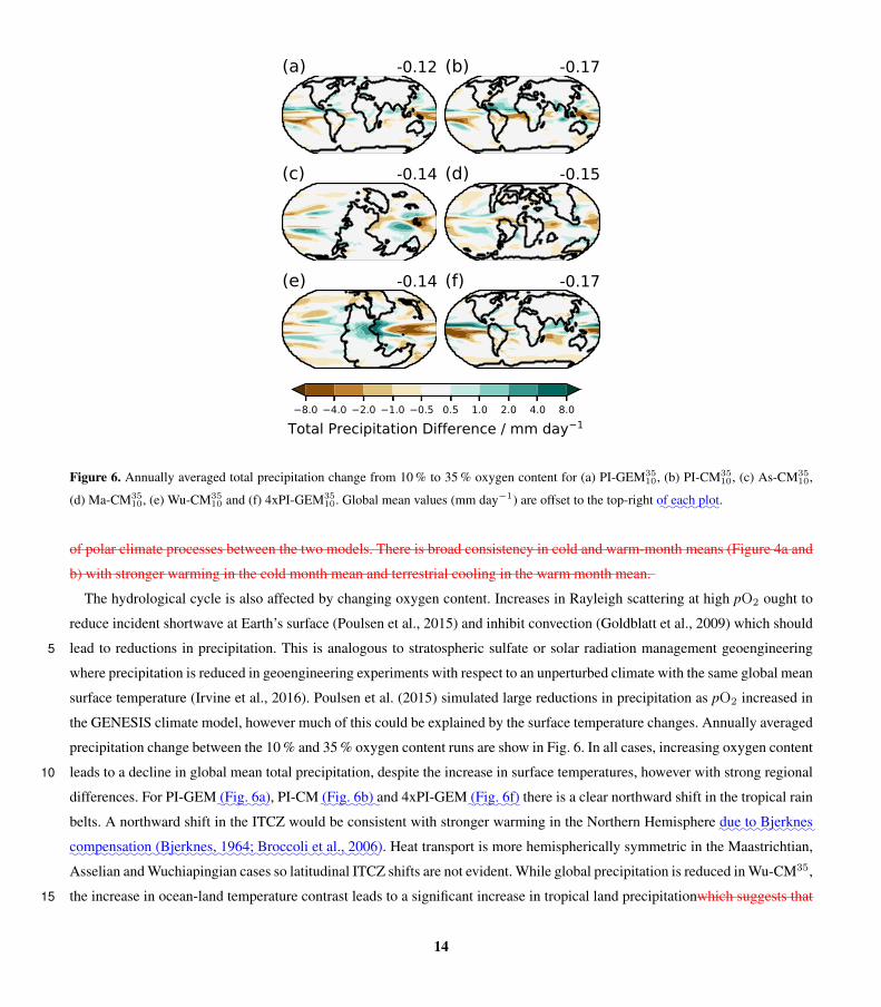
(a) -0.12 (b) -0.17

(c) -0.14 (d) -0.15

(e) -0.14 (f) -0.17

8.0 4.0 2.0 1.0 0.5 0.5 1.0 2.0 4.0 8.0Total Precipitation Difference / mm day 1

Figure 6. Annually averaged total precipitation change from 10 % to 35 % oxygen content for (a) PI-GEM3510, (b) PI-CM35

10, (c) As-CM3510,

(d) Ma-CM3510, (e) Wu-CM35

10 and (f) 4xPI-GEM3510. Global mean values (mm day−1) are offset to the top-right

:of

::::each

:::plot.

of polar climate processes between the two models. There is broad consistency in cold and warm-month means (Figure 4a and

b) with stronger warming in the cold month mean and terrestrial cooling in the warm month mean.

The hydrological cycle is also affected by changing oxygen content. Increases in Rayleigh scattering at high pO2 ought to

reduce incident shortwave at Earth’s surface (Poulsen et al., 2015) and inhibit convection (Goldblatt et al., 2009) which should

lead to reductions in precipitation. This is analogous to stratospheric sulfate or solar radiation management geoengineering5

where precipitation is reduced in geoengineering experiments with respect to an unperturbed climate with the same global mean

surface temperature (Irvine et al., 2016). Poulsen et al. (2015) simulated large reductions in precipitation as pO2 increased in

the GENESIS climate model, however much of this could be explained by the surface temperature changes. Annually averaged

precipitation change between the 10 % and 35 % oxygen content runs are show in Fig. 6. In all cases, increasing oxygen content

leads to a decline in global mean total precipitation, despite the increase in surface temperatures, however with strong regional10

differences. For PI-GEM::::(Fig.

:::6a), PI-CM

::::(Fig.

:::6b)

:and 4xPI-GEM

::::(Fig.

:::6f) there is a clear northward shift in the tropical rain

belts. A northward shift in the ITCZ would be consistent with stronger warming in the Northern Hemisphere:::due

::to

::::::::Bjerknes

:::::::::::compensation

:::::::::::::::::::::::::::::::(Bjerknes, 1964; Broccoli et al., 2006). Heat transport is more hemispherically symmetric in the Maastrichtian,

Asselian and Wuchiapingian cases so latitudinal ITCZ shifts are not evident. While global precipitation is reduced in Wu-CM35,

the increase in ocean-land temperature contrast leads to a significant increase in tropical land precipitationwhich suggests that15

14

pcould mediate monsoon circulations. Despite the increases in global-mean surface temperatures simulated for most cases,

precipitation is still reduced in all simulations.

:::::::::Comparing

:::the

:::::::surface


::::and

:::::::::::precipitation

::::::::response

:::::::between

::::::::::::HadCM3-BL

:::and

:::::::::::::HadGEM3-AO

::::::::suggests

::::that

::the

::::::model

:::::::::responses

:::are

:::::::broadly

:::::::::consistent.

::A

::::::::::::::::gridbox-by-gridbox

::::::::::comparison

:::of

::::::annual

:::::mean

::::::surface

:::air


::::and

::::::::::precipitation

:::::::::anomalies

:::for

:::::::::PI-GEM35

10 ::vs

::::::::PI-CM35

10::is

::::::::presented

::in

::::Fig.

:::S1.

::::The

:::::largest

:::::::::::discrepancy

::in

::::::surface

:::air

::::::::::temperature5

:::::::response

:::::::between

:::the

::::two

::::::models

::::::occurs

:::for

:::the

::::::largest


:::::::changes

:::::::::simulated

::by

:::::::::HadGEM,

::::::which

:::are

::::::::strongest

::in

:::::::Northern

:::::::::::Hemisphere

::::polar

:::::::regions.

::::This

:::::could

:::be

::::::linked

::to

:::::::::differences

::in:::

the::::::::::::

representation:::

of::::polar

:::::::climate

::::::::processes

::::and

:::::::::::amplification

::by

:::::polar

:::ice

:::::::::feedbacks

:::::::between

:::the

::::two

:::::::models.

:::::There

:::is

:::::broad

::::::::::consistency

::in

::::cold

::::and

:::::::::::warm-month

::::::means

::::::(Figure

::4a

::::and

::b)

::::with

:::::::stronger

::::::::warming

::in

:::the

:::cold

::::::month

:::::mean

:::and

::::::::terrestrial

:::::::cooling

::in

:::the

:::::warm

::::::month

:::::mean.

3.2 Energy Balance Decomposition10

The drivers of the changes in surface temperature can be understood by decomposing the terms which contribute to surface

temperature change in a 1D-energy balance model following Heinemann et al. (2009). For PI-CM3510, these results are shown

in Fig. 7. These show that the 1D-EBM can reasonably capture the temperature response in the HadCM3-BL simulations,

with slight errors (where the black and grey lines are not overlapping) evident in the polar regions. This could be due to

averaging over the polar rows in the HadCM3-BL model. There are positive contributions to the surface temperature change15

in the clear sky emissivity and albedo at the poles. This is consistent with the increase in pressure broadening of absorption

lines and the simulated reduction in sea-ice extent. By contrast, extrapolar contributions to clear sky albedo provide a negative

contribution to the temperature change which is consistent with an increase in Rayleigh scattering which would be expected

to be strongest in the tropics where the maximum in incoming solar radiation is located. Combined, the clear sky component

of the temperature change is +1.45◦C and the cloudy sky component is –0.35◦C. This suggests that HadCM3-BL supports a20

cloud feedback which acts to cool the climate at high pO2 and partially offset the clear-sky temperature changes.

The same analysis was performed for the HadGEM3-AO PIH simulations. Fig. 8 shows that a somewhat weaker cloud

feedback is simulated by HadGEM3-AO (–0.21◦C). Clear-sky contributions are slightly stronger (+1.51◦C). The largest dif-

ferences between the simulations appear in the all-sky albedo and emissivity changes, where there appear to be competing

factors which lead to a similar climate response possibly related to partitioning between the longwave and shortwave contri-25

butions to the cloud response. This is perhaps unsurprising, as cloud feedbacks to CO2 changes represent a large uncertainty

in future climate change projections and given the relatively small global-mean temperature changes a relatively small change

in cloud radiative effects has the power to considerably mediate the climate response. However the qualitative agreement in

latitudinal structure of the clear sky albedo and emissivity changes between these structurally different models gives some

confidence that the relevant climate feedbacks are well captured in these simulations.30

Analysis of the palaeo-case studies (As-CM, Fig. S2; Ma-CM, Fig. S3; Wu-CM, Fig. S4) shows a similar pattern. In all

simulations, irrespective of surface temperature response, the clear sky emissivity is a positive contribution to global mean

surface temperature change while clear sky albedo is a more negative contribution. The emissivity contribution becomes less

positive as pCO2 increases from As-CM to Ma-CM to Wu-CM. By contrast the albedo contribution becomes more negative

15

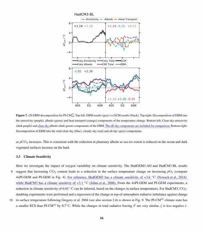
4

0

4

8

T sur

f / °C

+1.14 +1.10 +1.24 -0.25 +0.11

60S EQ 60N

4

0

4

8T s

urf /

°C

+2.36-1.02

60S EQ 60N

-0.35+1.45+1.10

HadCM3-BLEmissivity Albedo Heat Transport

Csky EmissivityCsky Albedo

Csky TotalCRE Total

GCMEBM

Figure 7. 1D-EBM decomposition for PI-CM3510. Top left: EBM results (grey) vs GCM results (black). Top right: Decomposition of EBM into

the emissivity (purple), albedo (green) and heat transport (orange) components of the temperature change. Bottom left: Clear-sky emissivity

(dark purple) and::::::clear-sky

:albedo (dark green) components of the EBM.

:::The

::::::all-sky

:::::::::components

::are

:::::::included

::for

::::::::::comparison. Bottom right:

Decomposition of EBM into the total clear-sky (blue), cloudy-sky (red) and all-sky (grey) components.

as pCO2 increases. This is consistent with the reduction in planetary albedo as sea-ice extent is reduced on the ocean and dark

vegetated surfaces increase on the land.

3.3 Climate Sensitivity

Here we investigate the impact of oxygen variability on climate sensitivity. The HadGEM3-AO and HadCM3-BL results

suggest that increasing CO2 content leads to a reduction in the surface temperature change on increasing pO2 (compare5

4xPI-GEM and PI-GEM in Fig. 4).:::For

:::::::::reference,

:::::::::HadGEM3

::::has

:a:::::::

climate:::::::::sensitivity

:::of

::::+3.6

:

◦C::::::::::::::::::(Nowack et al., 2014)

::::while

:::::::::HadCM3

:::has

::a

::::::climate

:::::::::sensitivty

::of

::::+3.1

:

◦C::::::::::::::::(Johns et al., 2006).

:From the 4xPI-GEM and PI-GEM experiments, a

reduction in climate sensitivity of 0.65 ◦C can be inferred, based on the changes in surface temperatures. For HadCM3, CO2-

doubling experiments were performed and a regression of the change in top-of-atmosphere radiative imbalance against change

in surface temperature following Gregory et al. 2004 (see also section 2.4) is shown in Fig. 9. The PI-CM35 climate state has10

a smaller ECS than PI-CM10 by 0.7◦C. While the changes in total radiative forcing F are very similar, ξ is less negative (-

16

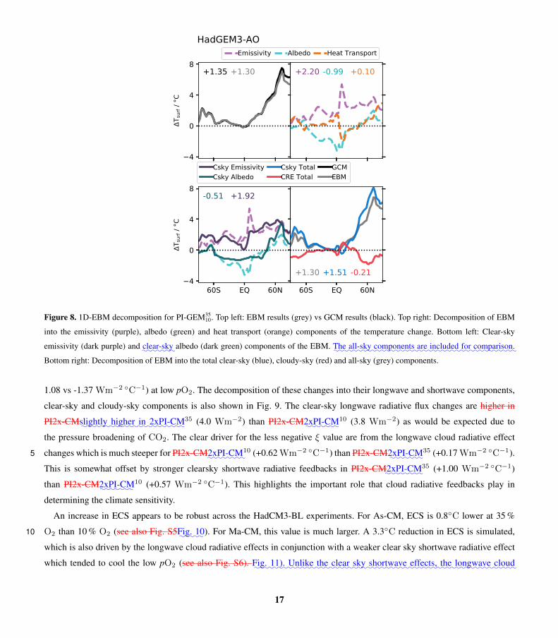
4

0

4

8

T sur

f / °C

+1.35 +1.30 +2.20 -0.99 +0.10

60S EQ 60N4

0

4

8T s

urf /

°C

+1.92-0.51

60S EQ 60N

-0.21+1.51+1.30

HadGEM3-AOEmissivity Albedo Heat Transport


Csky TotalCRE Total

GCMEBM

Figure 8. 1D-EBM decomposition for PI-GEM3510. Top left: EBM results (grey) vs GCM results (black). Top right: Decomposition of EBM

into the emissivity (purple), albedo (green) and heat transport (orange) components of the temperature change. Bottom left: Clear-sky

emissivity (dark purple) and:::::::clear-sky albedo (dark green) components of the EBM.

:::The

:::::all-sky

:::::::::components

:::are

:::::::included

::for

::::::::::comparison.

Bottom right: Decomposition of EBM into the total clear-sky (blue), cloudy-sky (red) and all-sky (grey) components.

1.08 vs -1.37 Wm−2 ◦C−1) at low pO2. The decomposition of these changes into their longwave and shortwave components,

clear-sky and cloudy-sky components is also shown in Fig. 9. The clear-sky longwave radiative flux changes are higher in

PI2x-CM::::::slightly

:::::higher

:::in

::::::::2xPI-CM35 (4.0 Wm−2) than PI2x-CM

:::::::2xPI-CM10 (3.8 Wm−2) as would be expected due to

the pressure broadening of CO2. The clear driver for the less negative ξ value are from the longwave cloud radiative effect

changes which is much steeper for PI2x-CM::::::::2xPI-CM10 (+0.62 Wm−2 ◦C−1) than PI2x-CM

:::::::2xPI-CM35 (+0.17 Wm−2 ◦C−1).5

This is somewhat offset by stronger clearsky shortwave radiative feedbacks in PI2x-CM::::::::2xPI-CM35 (+1.00 Wm−2 ◦C−1)

than PI2x-CM:::::::2xPI-CM10 (+0.57 Wm−2 ◦C−1). This highlights the important role that cloud radiative feedbacks play in

determining the climate sensitivity.

An increase in ECS appears to be robust across the HadCM3-BL experiments. For As-CM, ECS is 0.8◦C lower at 35 %

O2 than 10 % O2 (see also Fig. S5:::Fig.

::10). For Ma-CM, this value is much larger. A 3.3◦C reduction in ECS is simulated,10

which is also driven by the longwave cloud radiative effects in conjunction with a weaker clear sky shortwave radiative effect

which tended to cool the low pO2 (see also Fig. S6).:::Fig.

::::11).

::::::Unlike

:::the

::::clear

::::sky

:::::::::shortwave

::::::effects,

:::the

:::::::::longwave

:::::cloud

17

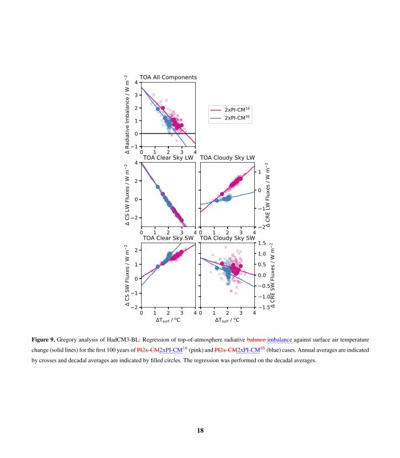
0 1 2 3 41

0

1

2

3

4

Rad

iativ

e Im

bala

nce

/ W m

2 TOA All Components

2xPI-CM10

2xPI-CM35

0 1 2 3 4

2

0

2

4

CS

LW F

luxe

s / W

m2

TOA Clear Sky LW

0 1 2 3 42

1

0

1

CRE

LW

Flu

xes /

W m

2

TOA Cloudy Sky LW

0 1 2 3 4Tsurf / oC

2

1

0

1

2

CS

SW F

luxe

s / W

m2

TOA Clear Sky SW

0 1 2 3 4Tsurf / oC

1.51.00.5

0.00.51.01.5

CRE

SW

Flu

xes /

W m

2

TOA Cloudy Sky SW

Figure 9. Gregory analysis of HadCM3-BL: Regression of top-of-atmosphere radiative balance::::::::imbalance against surface air temperature

change (solid lines) for the first 100 years of PI2x-CM:::::::2xPI-CM10 (pink) and PI2x-CM

:::::::2xPI-CM35 (blue) cases. Annual averages are indicated

by crosses and decadal averages are indicated by filled circles. The regression was performed on the decadal averages.

18

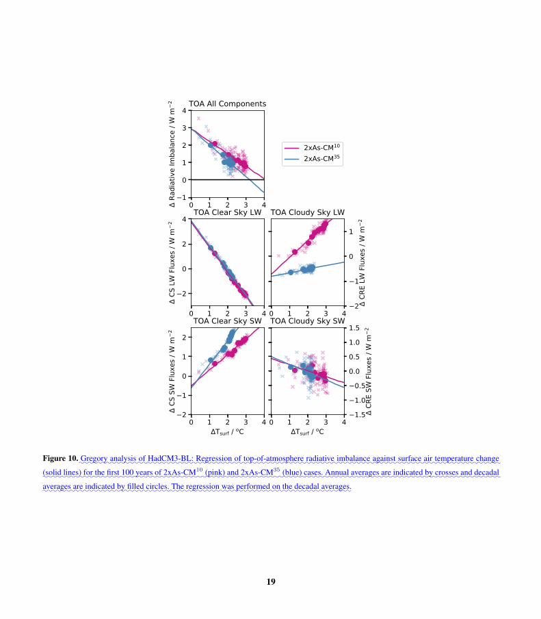
0 1 2 3 41

0

1

2

3

4

Rad

iativ

e Im

bala

nce

/ W m


2xAs-CM10

2xAs-CM35

0 1 2 3 4

2

0

2

4

CS

LW F

luxe

s / W

m2

TOA Clear Sky LW

0 1 2 3 42

1

0

1

CRE

LW

Flu

xes /

W m

2

TOA Cloudy Sky LW

0 1 2 3 4Tsurf / oC

2

1

0

1

2

CS

SW F

luxe

s / W

m2

TOA Clear Sky SW

0 1 2 3 4Tsurf / oC

1.51.00.5

0.00.51.01.5

CRE

SW

Flu

xes /

W m

2

TOA Cloudy Sky SW

Figure 10.::::::Gregory

:::::::analysis

::of

::::::::::HadCM3-BL:

:::::::::Regression

::of

::::::::::::::top-of-atmosphere

::::::radiative

::::::::imbalance

::::::against

::::::surface

::air


::::::change

::::(solid

:::::lines)

::for

:::the

:::first

:::100

::::years

::of

:::::::::2xAs-CM10

:::::(pink)

:::and

:::::::::2xAs-CM35

:::::(blue)

:::::cases.

::::::Annual

::::::averages

:::are

:::::::indicated

::by

::::::crosses

:::and

::::::decadal

::::::averages

:::are

:::::::indicated

::by

::::filled

::::::circles.

:::The

::::::::regression

:::was

::::::::performed

::on

:::the

::::::decadal

:::::::averages.

19

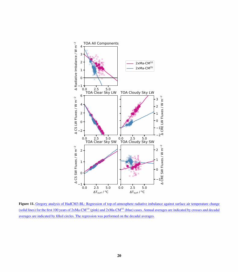
0.0 2.5 5.01

0

1

2

3

4

Rad

iativ

e Im

bala

nce

/ W m


2xMa-CM10

2xMa-CM35

0.0 2.5 5.0

2

0

2

4

6

CS

LW F

luxe

s / W

m2

TOA Clear Sky LW

0.0 2.5 5.02

1

0

1

2

3

CRE

LW

Flu

xes /

W m

2

TOA Cloudy Sky LW

0.0 2.5 5.0Tsurf / oC

1

0

1

2

CS

SW F

luxe

s / W

m2

TOA Clear Sky SW

0.0 2.5 5.0Tsurf / oC

1

0

1

2

CRE

SW

Flu

xes /

W m

2

TOA Cloudy Sky SW

Figure 11.::::::Gregory

:::::::analysis

::of

::::::::::HadCM3-BL:

:::::::::Regression

::of

::::::::::::::top-of-atmosphere

::::::radiative

::::::::imbalance

::::::against

::::::surface

::air


::::::change

::::(solid

::::lines)

:::for

:::the

:::first

:::100

::::years

::of

:::::::::2xMa-CM10

:::::(pink)

:::and

::::::::::2xMa-CM35

:::::(blue)

::::cases.

::::::Annual

::::::averages

:::are

:::::::indicated

::by

::::::crosses

:::and

::::::decadal

::::::averages

:::are

:::::::indicated

::by

::::filled

::::::circles.

:::The

::::::::regression

:::was

::::::::performed

::on

:::the

::::::decadal

:::::::averages.

20

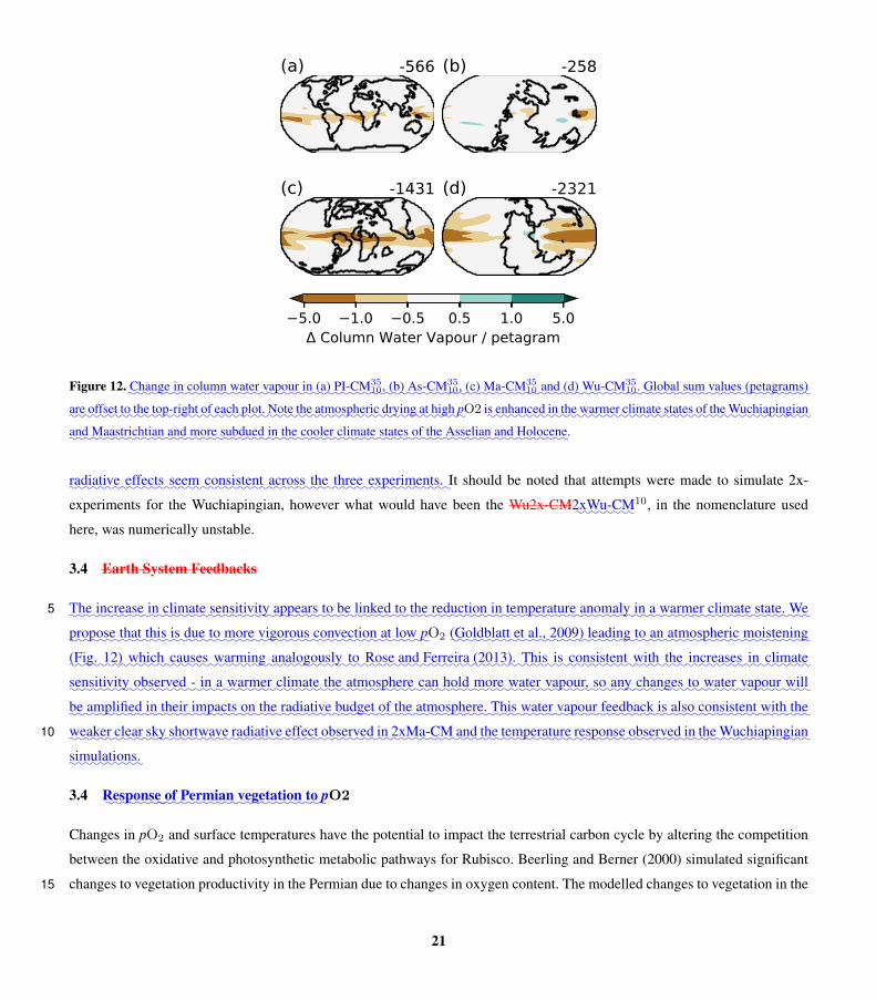
(a) -566 (b) -258

(c) -1431 (d) -2321

5.0 1.0 0.5 0.5 1.0 5.0 Column Water Vapour / petagram

Figure 12.::::::Change

::in

:::::column

:::::water

:::::vapour

::in

:::(a)

:::::::PI-CM35

10,:::(b)

::::::::As-CM35

10,::(c)

::::::::Ma-CM35

10:::and

::(d)

:::::::::Wu-CM35

10.:::::Global

::::sum

:::::values

:::::::::(petagrams)

::are

:::::offset

:to:::the

:::::::top-right

:of::::each

::::plot.

::::Note

::the

:::::::::atmospheric

:::::drying

::at

::::high

:pO2

:is

:::::::enhanced

::in

::the

::::::warmer

::::::climate

::::states

::of

::the

::::::::::::Wuchiapingian

:::and

::::::::::Maastrichtian

:::and

::::more

:::::::subdued

:in:::the

:::::cooler

::::::climate

::::states

::of

:::the

::::::Asselian

::::and

:::::::Holocene.

:::::::radiative

::::::effects

:::::seem

::::::::consistent

::::::across

:::the

:::::three

:::::::::::experiments.

:It should be noted that attempts were made to simulate 2x-

experiments for the Wuchiapingian, however what would have been the Wu2x-CM::::::::2xWu-CM10, in the nomenclature used

here, was numerically unstable.

3.4 Earth System Feedbacks

:::The

:::::::increase

::in

:::::::climate

::::::::sensitivity

:::::::appears

::to

::be

::::::linked

::to

:::the

::::::::reduction

::in


:::::::anomaly

:::in

:a:::::::warmer

::::::climate

:::::state.

:::We5

::::::propose

::::that

:::this

::is

::::due

::to

::::more

::::::::vigorous

:::::::::convection

::at

:::low

::pO2 :::::::::::::::::::

(Goldblatt et al., 2009)::::::leading

::to

::an

::::::::::atmospheric

::::::::::moistening

::::(Fig.

:::12)

::::::which

::::::causes

::::::::warming

::::::::::analogously

:::to

::::::::::::::::::::Rose and Ferreira (2013)

:.::::This

::is:::::::::

consistent::::with

::::the

::::::::increases

::in

:::::::climate

::::::::sensitivity

::::::::observed

:-::in::

a:::::::warmer

::::::climate

:::the

::::::::::atmosphere

:::can

:::::hold

::::more

:::::water

:::::::vapour,

::so

::::any

:::::::changes

::to

:::::water

::::::vapour

::::will

::be

::::::::amplified

::in

::::their

:::::::impacts

::on

:::the

::::::::radiative

::::::budget

::of

:::the

::::::::::atmosphere.

::::This

:::::water

::::::vapour

::::::::feedback

::is

:::also

:::::::::consistent

::::with

:::the

::::::weaker

::::clear

:::sky

:::::::::shortwave

:::::::radiative

:::::effect

::::::::observed

:in:::::::::2xMa-CM

::::and

::the


::::::::response

:::::::observed

::in:::the

:::::::::::::Wuchiapingian10

::::::::::simulations.

3.4::::::::Response

:::of

:::::::Permian

::::::::::vegetation

::to

:pO2

Changes in pO2 and surface temperatures have the potential to impact the terrestrial carbon cycle by altering the competition

between the oxidative and photosynthetic metabolic pathways for Rubisco. Beerling and Berner (2000) simulated significant

changes to vegetation productivity in the Permian due to changes in oxygen content. The modelled changes to vegetation in the15

21

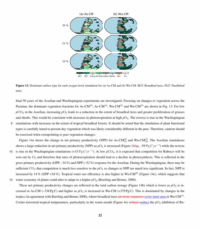
(a) As-CM

35 %

21 %

10 %

(b) Wu-CM

BLT NLT Grass ShrubsUrban Water Soil Ice

Figure 13. Dominant surface type for each oxygen level simulation for (a) As-CM and (b) Wu-CM. BLT: Broadleaf trees, NLT: Needleleaf

trees.

final 50 years of the Asselian and Wuchiapingian experiments are investigated. Focusing on changes to vegetation across the

Permian, the dominant vegetation fractions for As-CM35, As-CM10, Wu-CM35 and Wu-CM10 are shown in Fig. 13. For low

pCO2 in the Asselian, increasing pO2 leads to a reduction in the extent of broadleaf trees and greater proliferation of grasses

and shrubs. This would be consistent with increases in photorespiration at high pO2. The reverse is true in the Wuchiapingian

simulations with increases in the extent of tropical broadleaf forests. It should be noted that the simulation of plant functional5

types is carefully tuned to present day vegetation which was likely considerably different in the past. Therefore, caution should

be exercised when extrapolating to past vegetation changes.

Figure 14a shows the change in net primary productivity (NPP) for As-CM3510 and Wu-CM35

10. The Asselian simulations

shows a large reduction in net primary productivity (NPP) as pO2 is increased (Figure 14A:a, –59 Pg C yr−1) while the reverse

is true in the Wuchiapingian simulations (+33 Pg C yr−1). At low pCO2, it is expected that competition for Rubisco will be10

won out by O2 and therefore that rates of photorespiration should lead to a decline in photosynthesis. This is reflected in the

gross primary productivity (GPP, –34 %) and NPP (–52 %) response for the Asselian. During the Wuchiapingian, there may be

sufficient CO2 that competition is much less sensitive to the pO2 so changes to NPP are much less significant. In fact, NPP is

increased by 14 % (GPP +18 %). Tropical water use efficiency is also higher in Wu-CM35 (Figure 14c), which suggests that

water economy of plants could alter to adapt to a higher pO2 (Beerling and Berner, 2000).15

These net primary productivity changes are reflected in the total carbon storage (Figure 14b) which is lower as pO2 is in-

creased in As-CM (–338 Pg C) and higher as pO2 is increased in Wu-CM (+379 Pg C). This is dominated by changes in the

tropics (in agreement with Beerling and Berner 2000), where broadleaf trees are more expansive::::cover

:::::more

::::area in Wu-CM35.

Cooler terrestrial tropical temperatures, particularly in the warm month (Figure 4e) reduces::::::reduce the pO2 inhibition of Ru-

22

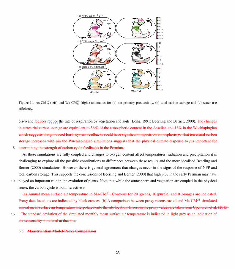
(a) NPP / g m 2 s 1

80402010

10204080

(b) C Storage / kg m 2

10

5

1

1

5

10

(c) WUE / gC kg(H2O) 1

As-CM Wu-CM 10

5

1

1

5

10

Figure 14. As-CM3510 (left) and Wu-CM35

10 (right) anomalies for (a) net primary productivity, (b) total carbon storage and (c) water use

efficiency.

bisco and reduces:::::reduce

:the rate of respiration by vegetation and soils (Long, 1991; Beerling and Berner, 2000). The changes

in terrestrial carbon storage are equivalent to 56 % of the atmospheric content in the Asselian and 16% in the Wuchiapingian

which suggests that pinduced Earth system feedbacks could have significant impacts on atmospheric p. That terrestrial carbon

storage increases with pin the Wuchiapingian simulations suggests that the physical climate response to pis important for

determining the strength of carbon cycle feedbacks in the Permian.5

As these simulations are fully coupled and changes to oxygen content affect temperatures, radiation and precipitation it is

challenging to explore all the possible contributions to differences between these results and the more idealised Beerling and

Berner (2000) simulations. However, there is general agreement that changes occur in the signs of the response of NPP and

total carbon storage. This supports the conclusions of Beerling and Berner (2000) that high pO2 in the early Permian may have

played an important role in the evolution of plants. Note that while the atmosphere and vegetation are coupled in the physical10

sense, the carbon cycle is not interactive .

(a) Annual mean surface air temperature in Ma-CM21. Contours for 20 (green), 10 (purple) and 0 (orange) are indicated.

Proxy data locations are indicated by black crosses. (b) A comparison between proxy reconstructed and Ma-CM21 simulated

annual mean surface air temperature interpolated onto the site location. Errors in the proxy values are taken from Upchurch et al. (2015)

. The standard deviation of the simulated monthly mean surface air temperature is indicated in light grey as an indication of15

the seasonality simulated at that site.

3.5 Maastrichtian Model-Proxy Comparison

23

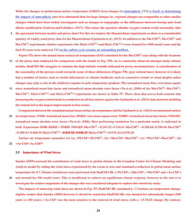
While the changes to global-mean surface temperature (GMST) from changes in::::::::::(atmospheric

:CO2

:is

:::::fixed)

::so

:::::::::::determining

::the

:::::::impacts

::of:::::::::::

atmospheric pare less substantial than for large changes in , regional changes are comparable to other smaller

changes which have been widely investigated such as changes to topography or the differences between forcing and cloud

albedo modification (Carlson and Caballero, 2017). This raises the question whether oxygen content could reasonably alter

the agreement between models and proxy data? For this we employ the Maastrichtian experiments as there is a considerable5

quantity of widely used proxy data for the Maastrichtian (Upchurch et al., 2015). In addition to the Ma-CM35, Ma-CM21 and

Ma-CM10 experiments, further experiments (the Ma2x-CM35* and Ma2x-CM10*) were iterated for 1000 model years and the

final 50 years were analysed. O2::on

:::the

::::::carbon

::::cycle

:::::::remains

:::an

:::::::::outstanding

::::::::problem.

:

Figure ??a shows the annual mean surface air temperature (SAT) simulated for the Ma-CM21 case along with the locations

of the proxy data employed for comparison with the model in Fig. ??b. As is commonly observed amongst many climate10

models, HadCM3-BL struggles to simulate the high latitude warmth indicated by proxy reconstructions. A consideration of

the seasonality of the proxies could reconcile some of these differences (Figure ??b, grey vertical bars), however it is likely

that a number of factors such as model deficiencies or climate feedbacks such as convective clouds or cloud droplet radius

changes may play a role in the shallower equator-to-pole temperature gradient. The normalised mean bias, root mean square

error, normalised mean bias factor and normalised mean absolute error factor (Yu et al., 2006) of the Ma-CM35, Ma-CM21,15

Ma-CM10, Ma2x-CM10* and Ma2x-CM35* experiments are shown in Table ??. These show that across both contents that

increasing the oxygen content leads to a reduction in all bias metrics against the Upchurch et al. (2015) data, however doubling

the content led to the largest improvement in bias scores.

Comparison between the simulated annual mean surface air temperature and the Upchurch et al. (2015) reconstructed surface

air temperature. NMB: normalised mean bias. RMSE: root mean square error. NMBF: normalised mean bias factor. NMAEF:20

normalised mean absolute error factor (Yu et al., 2006). Best performing simulation for a particular metric is indicated in

bold. Experiment NMB RMSE / NMBF NMAEF Ma-CM35 –0.247.92–0.310.41 Ma-CM21 –0.288.68–0.390.48 Ma-CM10

–0.288.83–0.400.50 Ma2x-CM35* –0.045.82–0.040.25 Ma2x-CM10* +0.076.22+0.070.26

Surface air temperature anomalies for (a) τPI-CM*–PI-CM21, (b) τMa-CM*–Ma-CM21, (c) τWu-CM*–Wu-CM21, (d)

τAs-CM*–As-CM2125

3.5 Importance of Wind Stress

Saenko (2009) assessed the contribution of wind stress to global climate in the Canadian Centre for Climate Modeling and

Analysis model by setting the wind stress experienced by the ocean to zero and simulated a reduction in global mean surface

temperature by 8.7. Similar simulations were performed with HadCM3-BL (τPI-CM*, τMa-CM*, τWu-CM* and τAs-CM*)

and iterated for 500 model years. This is insufficient to achieve an equilibrium climate response, however as the aim is to30

investigate the relative magnitude of the changes this was considered adequate to explore this sensitivity study.

The impacts of removing wind stress are shown in Fig. ??. HadCM3-BL simulated a –7.3surface air temperature change,

slightly weaker than Saenko (2009) however it should be noted that HadCM3-BL was iterated for substantially longer (500

years vs 100 years). τAs-CM* was the most sensitive to the removal of wind stress, with a –15.7SAT change. By contrast,

24

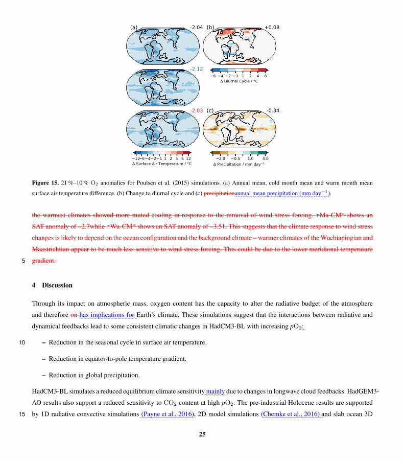
(a) -2.04

-2.12

-2.03

12 6 4 2 1 1 2 4 6 12 Surface Air Temperature / °C

(b) +0.08

6 4 2 1 1 2 4 6 Diurnal Cycle / °C

(c) -0.34

2.0 0.5 1.0 4.0 Precipitation / mm day 1

Figure 15. 21 %–10 % O2 anomalies for Poulsen et al. (2015) simulations. (a) Annual mean, cold month mean and warm month mean

surface air temperature difference. (b) Change to diurnal cycle and (c) precipitation:::::annual

::::mean

::::::::::precipitation

:::(mm

::::::day−1).

the warmest climates showed more muted cooling in response to the removal of wind stress forcing. τMa-CM* shows an

SAT anomaly of –2.7while τWu-CM* shows an SAT anomaly of –3.51. This suggests that the climate response to wind stress

changes is likely to depend on the ocean configuration and the background climate – warmer climates of the Wuchiapingian and

Maastrichtian appear to be much less sensitive to wind stress forcing. This could be due to the lower meridional temperature

gradient.5

4 Discussion

Through its impact on atmospheric mass, oxygen content has the capacity to alter the radiative budget of the atmosphere

and therefore on:::has

::::::::::implications

:::for

:Earth’s climate. These simulations suggest that the interactions between radiative and

dynamical feedbacks lead to some consistent climatic changes in HadCM3-BL with increasing pO2::

– Reduction in the seasonal cycle in surface air temperature.10

– Reduction in equator-to-pole temperature gradient.

– Reduction in global precipitation.

HadCM3-BL simulates a reduced equilibrium climate sensitivity::::::mainly due to changes in longwave cloud feedbacks. HadGEM3-

AO results also support a reduced sensitivity to CO2 content at high pO2. The pre-industrial Holocene results are supported

by 1D radiative convective simulations::::::::::::::::(Payne et al., 2016), 2D model simulations

::::::::::::::::::(Chemke et al., 2016) and slab ocean 3D15

25

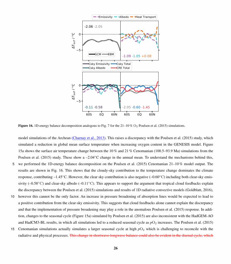
5

0

T sur

f / °C

-2.06 -2.05

-1.09 -1.05 +0.08

60S EQ 60N

5

0

T sur

f / °C

-0.58-0.11

60S EQ 60N

-1.45-0.60-2.05

Emissivity Albedo Heat Transport

GCM EBM


Csky TotalCRE Total

Figure 16. 1D-energy balance decomposition analogous to Fig. 7 for the 21–10 % O2 Poulsen et al. (2015) simulations.

model simulations of the Archean:::::::::::::::::(Charnay et al., 2013). This raises a discrepancy with the Poulsen et al. (2015) study, which

simulated a reduction in global mean surface temperature when increasing oxygen content in the GENESIS model. Figure

15a shows the surface air temperature change between the 10 % and 21 % Cenomanian (100.5–93.9 Ma) simulations from the

Poulsen et al. (2015) study. These show a –2.04◦C change in the annual mean. To understand the mechanisms behind this,

we performed the 1D-energy balance decomposition on the Poulsen et al. (2015) Cenomanian 21–10 % model output. The5

results are shown in Fig. 16. This shows that the cloudy-sky contribution to the temperature change dominates the climate

response, contributing –1.45◦C. However, the clear sky contribution is also negative (–0.60◦C) including both clear-sky emis-

sivity (–0.58◦C) and clear-sky albedo (–0.11◦C). This appears to support the argument that tropical cloud feedbacks explain

the discrepancy between the Poulsen et al. (2015) simulations and results of 1D radiative convective models (Goldblatt, 2016),

however this cannot be the only factor. An increase in pressure broadening of absorption lines would be expected to lead to10

a positive contribution from the clear-sky emissivity. This suggests that cloud feedbacks alone cannot explain the discrepancy

and that the implementation of pressure broadening may play a role in the anomalous Poulsen et al. (2015) response. In addi-

tion, changes to the seasonal cycle (Figure 15a) simulated by Poulsen et al. (2015) are also inconsistent with the HadGEM-AO

and HadCM3-BL results, in which all simulations led to a reduced seasonal cycle as pO2 increases. The Poulsen et al. (2015)

Cenomanian simulations actually simulates a larger seasonal cycle at high pO2 which is challenging to reconcile with the15

radiative and physical processes. This change in shortwave-longwave balance could also be evident in the diurnal cycle, which

26

ought to be weaker at high for the same reasons as the seasonal cycle, however this increases between 10 % and 21 % in the

Poulsen et al. (2015) simulation. Sub-daily data was not available from the HadCM3-BL or HadGEM3-AO simulations for

comparison. Note that the:::::::::::::::::Poulsen et al. (2015) simulations were for an earlier Cretaceous period

::::::::::::(Cenomanian) than those

performed in HadCM3-BL , the Maastrichtian. However, as employed a slab ocean the heat transport is fixed so ocean heat

transport changes caused by changes in continental configuration will not have been simulated:::::::::::::(Maastrichtian),

::::::::however

:::the5

:::::::::continental

::::::::::::configurations

::::and

:::the

:::::global

:::::mean

:::::::::::temperatures

:::are

::::::::::reasonably

::::::similar

:::::(22.2 ◦

::C

::in

:::::::::::HadCM3-BL

::vs

:::::20.5 ◦

::C

::in

:::::::::::::::::Poulsen et al. (2015)).

The simulations presented in here suggest that perturbations to the wind-driven ocean circulation by increasing atmospheric

mass leads to warmer temperatures, particularly at high latitudes. The magnitude of the results varies depending on the precise

continental configuration and background climate state. Gyre circulations vary between the preindustrial and the Maastrichtian10

and Asselian case studies. Given the importance of the wind-driven ocean circulation response this suggests that a 3D repre-

sentation of ocean circulation is necessary in order to capture the temperature response to atmospheric mass changes. It should

be noted however that Charnay et al. (2013) simulated higher surface temperatures for the early Earth at high atmospheric mass

with a slab ocean model.

The use of 3D oceans is now widespread in the palaeoclimate community, however this is not widely used in the exo-15

planet/early earth community (e.g. Kilic et al. 2017) and for early Earth studies such as the Archean (e.g. Charnay et al. 2013).

While boundary conditions for these studies are sparse or in some cases non-existent the additional uncertainty associated

with using a slab ocean should be considered. AO-GCM studies remain the best way to assess the complex coupling between

potentially competing radiative and dynamical effects.

Increased oxygen content may also contribute to explaining the very low temperature gradients for hothouse climates in20

the Phanerozoic – the “shallow gradients paradox” (Huber and Caballero, 2011). However, there are other mechanisms which

could lead to similar changes. Increases in the effective radii of liquid clouds leads to considerable warming, particularly at

high latitudes. While the tropics also warm the equator-to-pole temperature gradient is reduced. Abbot and Tziperman (2008)

describe a convective cloud feedback which warms the high latitudes, particularly in winter. Upchurch et al. (2015) found that

CCSM3 is able to reasonably simulate the shallow Maastrichtian temperature gradient when the effective radii of cloud droplets25

was set to 17 globally (comapred to typical values today around 8 over land surfaces and 14 over ocean surfaces and 17 only

observed for the most pristine of clouds in the current atmosphere), however this is hard to reconcile with the high primary

productivity likely in hothouse climates and the large contributions of biogenic sources of volatile organic compounds and

ammonia in the pre-industrial atmosphere (Gordon et al., 2017). In addition, the seasonality of cloud droplet changes is likely

to lead to the strongest temperature changes in the warm months which may increase lead to unreasonably high temperature30

changes in the tropics.

One criticism of high oxygen variability in the Phanerozoic is the possibility of runaway fire at high oxygen contents

(Watson et al., 1978). While subsequent experiments have put this in doubt::::::::::::::::::(Wildman et al., 2004), fire is undoubtedly a

negative feedback on oxygen content. However, the cooling of warmest month temperatures over tropical and midlatitude

continents in Wu-CM35 may provide somewhat of a protective mechanism against runaway fire regimes taking hold. Lightning35

27

is a major cause of paleofire (Scott and Jones, 1994) so the reduction in convection at high pO2 would also lead to fewer

lightning strikes which would reduce fire initiation. In addition, higher fire risk could have favoured the evolution and spread

of more fire-resistant species (Robinson, 1990).

The simulations of Permian climate (As-CM and Wu-CM) also suggest a strong role for pO2 variability in the terrestrial

carbon cycle. However, there are many limitations to the modelling approach employed here. The plant functional types em-5

ployed here are the same as present day. In particular, C4 photosynthesis likely evolved in the Oligocene (Sage, 2004) although

there is evidence of vegetation which causes C4-like fractionation:in

:::the

::::::::::::Mississippian, suggesting different vegetation adap-

tations operating in the past (Jones, 1994). In addition, angiosperms did not evolve until the Cretaceous so gymnosperms such

as cycads were more widespread in the Permian (Taylor et al., 2009). TRIFFID and other dynamic plant models were not

developed with these changes in plant types in mind so simulating past vegetation changes is still a considerable challenge.10

However, scientific understanding of the role of plants in the climate in the Paleozoic is still immature. While early evidence

suggested that late Paleozoic vegetation was unproductive based on analysis of the closest modern relatives, this perspective is

increasingly being challenged (Wilson et al., 2017). Other approaches such as trait based methods (Van Bodegom et al., 2012)

:::::::::::::::::::::::::::::::::::::::(Van Bodegom et al., 2012; Porada et al., 2016) may be able to achieve more insights into the role of pO2 in the Earth system.

We also have not accounted for changes to the ocean carbon cycle. A biogeochemical model study suggests that pervasive15

oceanic anoxia and euxinia only occur below an oxygen level of around 10 % (Ozaki and Tajika, 2013) which may be below

the fire threshold (Belcher et al., 2010) and therefore not of relevance to many periods in the Phanerozoic. However, the extent

of oceanic anoxic events may be sensitive to atmospheric pO2 (Clarkson et al., 2018).

Given the relatively small contribution of to improving the proxy-model agreement for the Maastrichtian at the largest

oxygen changes and the small changes:::::small

:::::::changes

:in global mean surface temperature (GMST, 1.5 ◦C maximum) com-20

pared to ECS (~3 ◦C), this raises the question of how much pO2 variability contributes to uncertainty in Phanerozoic surface

temperature even with such large uncertainties in pO2 reconstructions. Figure 17 shows reconstructed Phanerozoic surface

temperatures based on CO2 content and climate sensitivity from the Geocarb model (purple, Royer et al. 2014). The un-

certainty associated with the 95% confidence interval in simulated pCO2 is also indicated (purple shading). Analysis of the

Poulsen et al. (2015) simulations suggests a global mean surface temperature reduction of 0.21 ◦C per percentage increase25

in O2. Accounting for the pO2 simulated by Royer et al. (2014) leads to a mean absolute difference in global mean surface

temperature of 0.80 ◦C and maximum absolute difference of 2.59 ◦C (Figure 17 orange line). The largest deviations from the

Geocarb values occur during the largest deviations from PAL:::::present

:::::::::::atmospheric

:::::levels

::of

:O2 during the Permian. However,

pO2 contributes little to the uncertainty in reconstruction of global mean surface temperature compared to pCO2 (Figure 17

orange dashed lines), even if the temperature changes simulated by Poulsen et al. (2015) are reasonable. The HadGEM3-AO30

and HadCM3-BL simulations show even less sensitivity of global mean surface temperature to pO2 changes which suggests

this is likely an overestimate.

pO2 therefore remains a secondary contribution to climatic variability in the Phanerozoic::in

:::::::::agreement

::::with

::::::::::::::::(Payne et al., 2016)

but most likely to be important during the Permian. The Artinskian (early Permian, 283.5–290.1 Ma) is associated with a rapid

increase in CO2 content from ~500 to ~3500 ppmv which is associated with considerable restructuring of tropical vegetation35

28

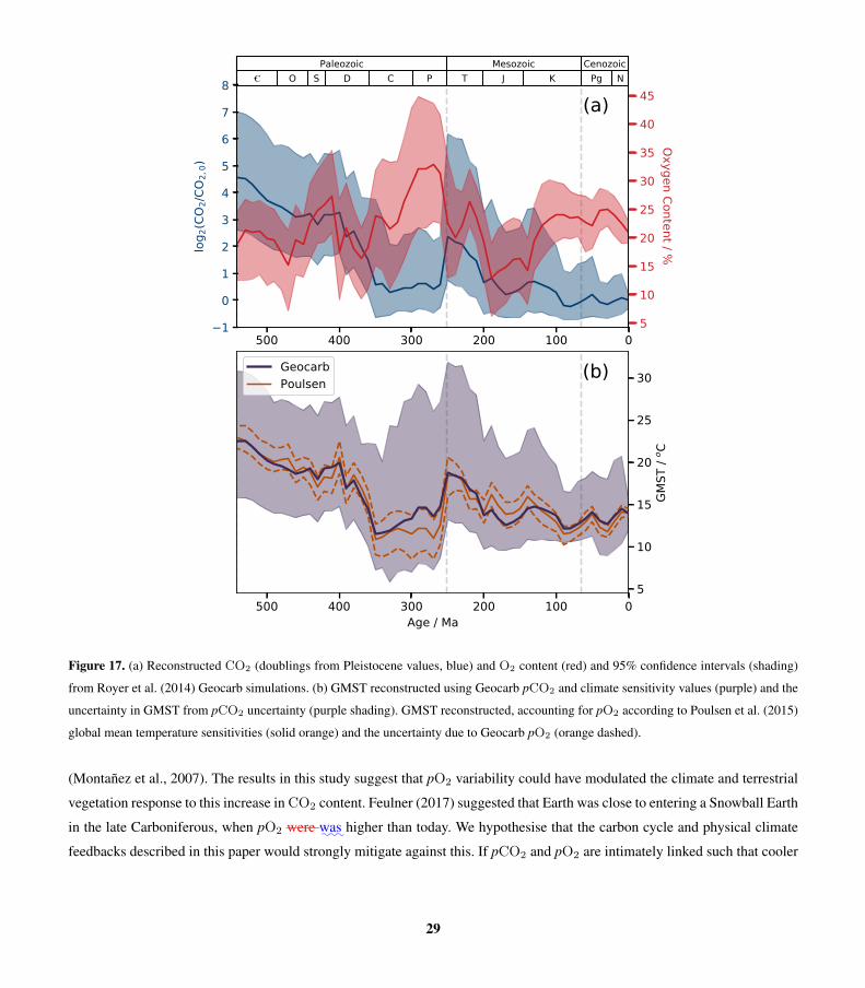
01002003004005001

0

1

2

3

4

5

6

7

8

log 2

(CO 2

/CO 2

,0)

(a)O S D C P T J K Pg N

Paleozoic Mesozoic Cenozoic

5

10

15

20

25

30

35

40

45

Oxygen Content / %

0100200300400500Age / Ma

5

10

15

20

25

30

GMST

/ o C

(b)GeocarbPoulsen

Figure 17. (a) Reconstructed CO2 (doublings from Pleistocene values, blue) and O2 content (red) and 95% confidence intervals (shading)

from Royer et al. (2014) Geocarb simulations. (b) GMST reconstructed using Geocarb pCO2 and climate sensitivity values (purple) and the

uncertainty in GMST from pCO2 uncertainty (purple shading). GMST reconstructed, accounting for pO2 according to Poulsen et al. (2015)

global mean temperature sensitivities (solid orange) and the uncertainty due to Geocarb pO2 (orange dashed).

(Montañez et al., 2007). The results in this study suggest that pO2 variability could have modulated the climate and terrestrial

vegetation response to this increase in CO2 content. Feulner (2017) suggested that Earth was close to entering a Snowball Earth

in the late Carboniferous, when pO2 were:::was higher than today. We hypothesise that the carbon cycle and physical climate

feedbacks described in this paper would strongly mitigate against this. If pCO2 and pO2 are intimately linked such that cooler

29

climates tends to increase pO2 this would suggest that pO2 responses have helped to prevent Snowball Earth initiation in the

Phanerozoic.

5 Conclusions

The numerical simulations performed in this study reconcile the surface temperature response to oxygen content changes across

the hierarchy of model complexity:5

– Under pre-industrial Holocene conditions, increasing atmospheric pO2 leads to an increase in global-mean surface tem-

perature in agreement with 1D radiative-convective model simulations. This increase is greater in the cold-month mean

than the warm month-mean. The equator-to-pole temperature gradient is reduced, particularly in the cold-month mean,

consistent with a stronger greenhouse effect at high atmospheric pressure.

– Lower incident surface shortwave radiation leads to a slow down of the hydrological cycle. Precipitation decreases10

globally under high pO2, with regional variations.

– The climate sensitivity is lower at high pO2, particularly in the Maastrichtian. This appears to reconcile the results of the

1D and 3D modelling approaches.

– For the Maastrichtian, model-proxy agreement is stronger at high pirrespective of p. Both simulations at 112 Pa agree

better with the Upchurch et al. (2015) proxy reconstruction than those at 56 Pa .15

– The climate response simulated by Poulsen et al. (2015) is inconsistent with the radiative changes when considering a

1D-energy balance model decomposition of the surface temperature changes. Tropical cloud feedbacks alone were not

sufficient to explain the discrepancy.

– The climate response to oxygen content variability is state-dependent so should be considered on a case-by-case basis.

However, the changes are relatively small compared to the role of CO2 in the Phanerozoic (Royer et al., 2014).20

Code and data availability. Processed model output and analysis scripts will be made available on the NERC data centre. The Met Office

Unified Model is available for use under licence. Please see http://www.metoffice.gov.uk/research/modelling-systems/unified-model for more

information. The ocean bathymetry and land orography reconstructions are ©Getech. Readers who would like advice on how to implement

alterations to pO2 in their climate model are encouraged to contact the corresponding authors. UM users can obtain the code changes for

these particular versions from the corresponding authors.25

Competing interests. The authors declare no competing interests.

30

Acknowledgements. DCW acknowledges support from a UK Natural Environment Research Council Doctoral Training Program studentship

(Ref 1502139). This work was carried out using the computational facilities of the Advanced Computing Research Centre, University of

Bristol http://www.bris.ac.uk/acrc/. We acknowledge use of the MONSooN system, a collaborative facility supplied under the Joint Weather

and Climate Research Programme, a strategic partnership between the Met Office and the Natural Environment Research Council. DCW

acknowledges Eric Wolff and David Stevenson for their comments on the PhD thesis from which this paper largely forms a part.5

31

References

Abbot, D. S. and Tziperman, E.: A high-latitude convective cloud feedback and equable climates, Quarterly Journal of the Royal Meteoro-

logical Society, 134, 165–185, https://doi.org/10.1002/qj.211, 2008.

Algeo, T. J. and Ingall, E.: Sedimentary Corg:P ratios, paleocean ventilation, and Phanerozoic atmospheric pO2, Palaeogeography, Palaeo-

climatology, Palaeoecology, 256, 130–155, https://doi.org/10.1016/J.PALAEO.2007.02.029, 2007.5

Armour, K. C., Bitz, C. M., and Roe, G. H.: Time-Varying Climate Sensitivity from Regional Feedbacks, Journal of Climate, 26, 4518–4534,

https://doi.org/10.1175/JCLI-D-12-00544.1, 2013.

Arvidson, R. S., Mackenzie, F. T., and Guidry, M. W.: Geologic history of seawater: A MAGic approach to carbon chemistry and ocean

ventilation, Chemical Geology, 362, 287–304, https://doi.org/10.1016/J.CHEMGEO.2013.10.012, 2013.

Awakawa, A. and Lamb, V. R.: Computational Design of the Basic Dynamical Processes of the UCLA General Circulation Model, Methods10

in Computational Physics: Advances in Research and Applications, 17, 173–265, 1977.

Banerjee, A., Archibald, A. T., Maycock, A., Telford, P., Abraham, N. L., Yang, X., Braesicke, P., and Pyle, J. A.: Lightning NOx, a

key chemistry–climate interaction: impacts of future climate change and consequences for tropospheric oxidising capacity, Atmospheric

Chemistry and Physics Discussions, 14, 8753–8778, https://doi.org/10.5194/acpd-14-8753-2014, 2014.

Beerling, D., Lake, J., Berner, R., Hickey, L., Taylor, D., and Royer, D.: Carbon isotope evidence implying high O2/CO2 ratios in the15

Permo-Carboniferous atmosphere, Geochimica et Cosmochimica Acta, 66, 3757–3767, https://doi.org/10.1016/S0016-7037(02)00901-8,

2002.

Beerling, D., Berner, R. A., Mackenzie, F. T., Harfoot, M. B., and Pyle, J. A.: Methane and the CH4-related greenhouse effect over the past

400 million years, American Journal of Science, 309, 97–113, https://doi.org/10.2475/02.2009.01, 2009.

Beerling, D. J. and Berner, R. A.: Impact of a Permo-Carboniferous high O2 event on the terrestrial carbon cycle., Proceedings of the National20

Academy of Sciences of the United States of America, 97, 12 428–32, https://doi.org/10.1073/pnas.220280097, 2000.

Beerling, D. J., Fox, A., Stevenson, D. S., and Valdes, P. J.: Enhanced chemistry-climate feedbacks in past greenhouse worlds., Proceedings

of the National Academy of Sciences of the United States of America, 108, 9770–9775, https://doi.org/10.1073/pnas.1102409108, 2011.

Belcher, C. M. and McElwain, J. C.: Limits for Combustion in Low O2 Redefine Paleoatmospheric Predictions for the Mesozoic, Science,

321, 1197–200, 2008.25

Belcher, C. M., Yearsley, J. M., Hadden, R. M., McElwain, J. C., and Rein, G.: Baseline intrinsic flammability of Earth’s ecosystems estimated

from paleoatmospheric oxygen over the past 350 million years., Proceedings of the National Academy of Sciences of the United States of

America, 107, 22 448–53, https://doi.org/10.1073/pnas.1011974107, 2010.

Bergman, N. M., Lenton, T. M., and Watson, A. J.: COPSE: A new model of biogeochemical cycling over Phanerozoic time, American

Journal of Science, 304, 397–437, https://doi.org/10.2475/ajs.304.5.397, 2004.30

Berner, R. A.: Phanerozoic atmospheric oxygen: New results using the GEOCARBSULF model, American Journal of Science, 309, 603–606,

https://doi.org/10.2475/07.2009.03, 2009.

Berner, R. A. and Canfield, D. E.: A new model for atmospheric oxygen over Phanerozoic time, American Journal of Science, 289, 333–361,

https://doi.org/10.2475/ajs.289.4.333, 1989.

Berner, R. A., Vandenbrooks, J. M., and Ward, P. D.: Evolution. Oxygen and evolution., Science, 316, 557–8,35

https://doi.org/10.1126/science.1140273, 2007.

32

Bjerknes, J.: Atlantic Air-Sea Interaction, 10, 1 – 82, https://doi.org/https://doi.org/10.1016/S0065-2687(08)60005-9, http://www.

sciencedirect.com/science/article/pii/S0065268708600059, 1964.

Bony, S., Stevens, B., Frierson, D. M. W., Jakob, C., Kageyama, M., Pincus, R., Shepherd, T. G., Sherwood, S. C., Siebesma,

A. P., Sobel, A. H., Watanabe, M., and Webb, M. J.: Clouds, circulation and climate sensitivity, Nature Geoscience, 8, 261–268,

https://doi.org/10.1038/ngeo2398, 2015.5

Brand, U., Posenato, R., Came, R., Affek, H., Angiolini, L., Azmy, K., and Farabegoli, E.: The end-Permian mass extinction: A rapid volcanic

CO2 and CH4-climatic catastrophe, Chemical Geology, 322-323, 121–144, 2012.

Breecker, D. O., Sharp, Z. D., and McFadden, L. D.: Atmospheric CO2 concentrations during ancient greenhouse climates were similar

to those predicted for A.D. 2100., Proceedings of the National Academy of Sciences of the United States of America, 107, 576–80,

https://doi.org/10.1073/pnas.0902323106, 2010.10

Broccoli, A. J., Dahl, K. A., and Stouffer, R. J.: Response of the ITCZ to Northern Hemisphere cooling, Geophysical Research Letters, 33,

https://doi.org/10.1029/2005GL024546, https://agupubs.onlinelibrary.wiley.com/doi/abs/10.1029/2005GL024546, 2006.

Budyko, M. I.: The effect of solar radiation variations on the climate of the Earth, Tellus, 21, 611–619,

https://doi.org/10.3402/tellusa.v21i5.10109, 1969.

Caballero, R. and Huber, M.: State-dependent climate sensitivity in past warm climates and its implications for future climate projections,15

Proceedings of the National Academy of Sciences, 110, 14 162–14 167, https://doi.org/10.1073/pnas.1303365110, 2013.

Carlson, H. and Caballero, R.: Atmospheric circulation and hydroclimate impacts of alternative warming scenarios for the Eocene, Climate

of the Past, 13, 1037–1048, https://doi.org/10.5194/cp-13-1037-2017, 2017.

Catling, D. C. and Claire, M. W.: How Earth’s atmosphere evolved to an oxic state: A status report, Earth and Planetary Science Letters, 237,

1–20, https://doi.org/10.1016/J.EPSL.2005.06.013, 2005.20

Catling, D. C., Glein, C. R., Zahnle, K. J., and McKay, C. P.: Why O2 Is Required by Complex Life on Habitable Planets and the Concept of

Planetary “Oxygenation Time”, Astrobiology, 5, 415–438, https://doi.org/10.1089/ast.2005.5.415, 2005.

Charnay, B., Forget, F., Wordsworth, R., Leconte, J., Millour, E., Codron, F., and Spiga, A.: Exploring the faint young Sun problem and

the possible climates of the Archean Earth with a 3-D GCM, Journal of Geophysical Research: Atmospheres, 118, 10,414–10,431,

https://doi.org/10.1002/jgrd.50808, 2013.25

Chemke, R., Kaspi, Y., and Halevy, I.: The thermodynamic effect of atmospheric mass on early Earth’s temperature, Geophysical Research

Letters, 43, 11,414–11,422, https://doi.org/10.1002/2016GL071279, 2016.

Clark, D. B., Mercado, L. M., Sitch, S., Jones, C. D., Gedney, N., Best, M. J., Pryor, M., Rooney, G. G., Essery, R. L. H., Blyth, E.,

Boucher, O., Harding, R. J., Huntingford, C., and Cox, P. M.: The Joint UK Land Environment Simulator (JULES), model description

âC“ Part 2: Carbon fluxes and vegetation dynamics, Geoscientific Model Development, 4, 701–722, https://doi.org/10.5194/gmd-4-701-30

2011, https://www.geosci-model-dev.net/4/701/2011/, 2011.

Clarkson, M. O., Stirling, C. H., Jenkyns, H. C., Dickson, A. J., Porcelli, D., Moy, C. M., Pogge von Strandmann, P. A. E., Cooke, I. R., and

Lenton, T. M.: Uranium isotope evidence for two episodes of deoxygenation during Oceanic Anoxic Event 2., Proceedings of the National

Academy of Sciences of the United States of America, 115, 2918–2923, https://doi.org/10.1073/pnas.1715278115, 2018.

Cox, P.: A primitive equation, 3-dimensional model of the ocean, GFDL Ocean Group Technical Report No. 1, Tech. rep., Geophysical Fluid35

Dynamics Laboratory, Princeton, New Jersey, 1984.

Cox, P., Huntingford, C., and Harding, R.: A canopy conductance and photosynthesis model for use in a GCM land surface scheme, Journal

of Hydrology, 212-213, 79–94, https://doi.org/10.1016/S0022-1694(98)00203-0, 1998.

33

Cox, P., Betts, R. A., Jones, C., A. Spall, S., and J. Totterdell, I.: Acceleration of global warming due to carbon-cycle feedbacks in a coupled

model, Nature, 408, 184–187, 2000.

Cox, P. M., Betts, R. A., Bunton, C. B., Essery, R. L. H., Rowntree, P. R., and Smith, J.: The impact of new land surface physics on the GCM

simulation of climate and climate sensitivity, Climate Dynamics, 15, 183–203, https://doi.org/10.1007/s003820050276, 1999.

Dahl, T. W., Hammarlund, E. U., Anbar, A. D., Bond, D. P. G., Gill, B. C., Gordon, G. W., Knoll, A. H., Nielsen, A. T., Schovsbo, N. H., and5

Canfield, D. E.: Devonian rise in atmospheric oxygen correlated to the radiations of terrestrial plants and large predatory fish, Proceedings

of the National Academy of Sciences, 107, 17 911–17 915, https://doi.org/10.1073/pnas.1011287107, https://www.pnas.org/content/107/

42/17911, 2010.

Davies, T., Cullen, M. J. P., Malcolm, A. J., Mawson, M. H., Staniforth, A., White, A. A., and Wood, N.: A new dynamical core for the

Met Office’s global and regional modelling of the atmosphere, Quarterly Journal of the Royal Meteorological Society, 131, 1759–1782,10

https://doi.org/10.1256/qj.04.101, 2005.

Dwyer, J. G., Biasutti, M., and Sobel, A. H.: Projected Changes in the Seasonal Cycle of Surface Temperature, Journal of Climate, 25,

6359–6374, https://doi.org/10.1175/JCLI-D-11-00741.1, 2012.

Edwards, C. T., Saltzman, M. R., Royer, D. L., and Fike, D. A.: Oxygenation as a driver of the Great Ordovician Biodiversification Event,

Nature Geoscience, 10, 925–929, https://doi.org/10.1038/s41561-017-0006-3, 2017.15

Edwards, J. M. and Slingo, A.: Studies with a flexible new radiation code. I: Choosing a configuration for a large-scale model, Quarterly

Journal of the Royal Meteorological Society, 122, 689–719, https://doi.org/10.1002/qj.49712253107, 1996.

Essery, R. L. H., Best, M. J., Betts, R. A., Cox, P. M., Taylor, C. M., Essery, R. L. H., Best, M. J., Betts, R. A., Cox, P. M., and Taylor,

C. M.: Explicit Representation of Subgrid Heterogeneity in a GCM Land Surface Scheme, Journal of Hydrometeorology, 4, 530–543,

https://doi.org/10.1175/1525-7541(2003)004<0530:EROSHI>2.0.CO;2, 2003.20

Falkowski, P. G., Katz, M. E., Milligan, A. J., Fennel, K., Cramer, B. S., Aubry, M. P., Berner, R. A., Novacek, M. J., and Zapol, W. M.: The

Rise of Oxygen over the Past 205 Million Years and the Evolution of Large Placental Mammals, Science, 309, 2005.

Feulner, G.: The faint young Sun problem, Reviews of Geophysics, 50, RG2006, https://doi.org/10.1029/2011RG000375, 2012.

Feulner, G.: Formation of most of our coal brought Earth close to global glaciation., Proceedings of the National Academy of Sciences of

the United States of America, 114, 11 333–11 337, https://doi.org/10.1073/pnas.1712062114, 2017.25

Finney, D. L., Doherty, R. M., Wild, O., Stevenson, D. S., MacKenzie, I. A., and Blyth, A. M.: A projected decrease in lightning under

climate change, Nature Climate Change, 8, 210–213, https://doi.org/10.1038/s41558-018-0072-6, 2018.

Forster, P. M. and Shine, K. P.: Radiative forcing and temperature trends from stratospheric ozone changes, Journal of Geophysical Research:

Atmospheres, 102, 10 841–10 855, https://doi.org/10.1029/96JD03510, 1997.

Franks, P. J., Royer, D. L., Beerling, D. J., Van de Water, P. K., Cantrill, D. J., Barbour, M. M., and Berry, J. A.: New constraints on30

atmospheric CO2 concentration for the Phanerozoic, Geophysical Research Letters, 41, 4685–4694, 2014.

Glasspool, I. J. and Scott, A. C.: Phanerozoic concentrations of atmospheric oxygen reconstructed from sedimentary charcoal, Nature Geo-

science, 3, 627–630, https://doi.org/10.1038/ngeo923, 2010.

Goldblatt, C.: Comment on “Long-term climate forcing by atmospheric oxygen concentrations”, Science, 353, 132, 2016.

Goldblatt, C., Claire, M. W., Lenton, T. M., Matthews, A. J., Watson, A. J., and Zahnle, K. J.: Nitrogen-enhanced greenhouse warming on35

early Earth, Nature Geoscience, 2, 891–896, https://doi.org/10.1038/ngeo692, 2009.

34

Gordon, C., Cooper, C., Senior, C. A., Banks, H., Gregory, J. M., Johns, T. C., Mitchell, J. F. B., and Wood, R. A.: The simulation of SST,

sea ice extents and ocean heat transports in a version of the Hadley Centre coupled model without flux adjustments, Climate Dynamics,

16, 147–168, https://doi.org/10.1007/s003820050010, 2000.

Gordon, H., Kirkby, J., Baltensperger, U., Bianchi, F., Breitenlechner, M., Curtius, J., Dias, A., Dommen, J., Donahue, N. M., Dunne, E. M.,

Duplissy, J., Ehrhart, S., Flagan, R. C., Frege, C., Fuchs, C., Hansel, A., Hoyle, C. R., Kulmala, M., Kürten, A., Lehtipalo, K., Makhmutov,5

V., Molteni, U., Rissanen, M. P., Stozkhov, Y., Tröstl, J., Tsagkogeorgas, G., Wagner, R., Williamson, C., Wimmer, D., Winkler, P. M.,

Yan, C., and Carslaw, K. S.: Causes and importance of new particle formation in the present-day and preindustrial atmospheres, Journal

of Geophysical Research: Atmospheres, 122, 8739–8760, https://doi.org/10.1002/2017JD026844, 2017.

Gregory, J. M., Ingram, W. J., Palmer, M. A., Jones, G. S., Stott, P. A., Thorpe, R. B., Lowe, J. A., Johns, T. C., and Williams,

K. D.: A new method for diagnosing radiative forcing and climate sensitivity, Geophysical Research Letters, 31, L03 205,10

https://doi.org/10.1029/2003GL018747, 2004.

Hadjinicolaou, P. and Pyle, J. A.: The Impact of Arctic Ozone Depletion on Northern Middle Latitudes: Interannual Variability and Dynamical

Control, Journal of Atmospheric Chemistry, 47, 25–43, https://doi.org/10.1023/B:JOCH.0000012242.06578.6c, 2004.

Hagemann, M., Weber, A. P., and Eisenhut, M.: Photorespiration: origins and metabolic integration in interacting compartments, Journal of

Experimental Botany, 67, 2915–2918, https://doi.org/10.1093/jxb/erw178, 2016.15

Haigh, J. D. and Pyle, J. A.: Ozone perturbation experiments in a two-dimensional circulation model, Quarterly Journal of the Royal Meteo-

rological Society, 108, 551–574, https://doi.org/10.1002/qj.49710845705, 1982.

Hansen, K. W. and Wallmann, K.: Cretaceous and Cenozoic evolution of seawater composition, atmospheric O2 and CO2: A model perspec-

tive, American Journal of Science, 303, 94–148, https://doi.org/10.2475/ajs.303.2.94, 2003.

Harfoot, M. B. J., Beerling, D. J., Lomax, B. H., and Pyle, J. a.: A two-dimensional atmospheric chemistry modeling investigation of20

Earth’s Phanerozoic O3 and near-surface ultraviolet radiation history, Journal of Geophysical Research: Atmospheres, 112, D07 308,

https://doi.org/10.1029/2006JD007372, 2007.

He, T., Pausas, J. G., Belcher, C. M., Schwilk, D. W., and Lamont, B. B.: Fire-adapted traits of Pinus arose in the fiery Cretaceous, New

Phytologist, 194, 751–759, 2012.

Heinemann, M.: Warm and sensitive Paleocene-Eocene Climate, Ph.D. thesis, Universität Hamburg, 2009.25

Heinemann, M., Jungclaus, J. H., and Marotzke, J.: Warm Paleocene/Eocene climate as simulated in ECHAM5/MPI-OM, Climate of the

Past, 5, 1297–1336, https://doi.org/10.5194/cpd-5-1297-2009, http://www.clim-past.net/5/785/2009/cp-5-785-2009.html, 2009.

Hewitt, H. T., Copsey, D., Culverwell, I. D., Harris, C. M., Hill, R. S. R., Keen, A. B., McLaren, A. J., and Hunke, E. C.: Design and

implementation of the infrastructure of HadGEM3: The next-generation Met Office climate modelling system, Geoscientific Model De-

velopment, 4, 223–253, https://doi.org/10.5194/gmd-4-223-2011, 2011.30

Huber, M. and Caballero, R.: The early Eocene equable climate problem revisited, Climate of the Past, 7, 603–633, https://doi.org/10.5194/cp-

7-603-2011, 2011.

Hunke, E. and Lipscomb, W.: The Los Alamos sea ice model documentation and software user’s manual, Version 4.0, LA-CC-06-012., Tech.

rep., Los Alamos National Laboratory„ 2008.

Irvine, P. J., Kravitz, B., Lawrence, M. G., and Muri, H.: An overview of the Earth system science of solar geoengineering, Wiley Interdisci-35

plinary Reviews: Climate Change, 7, 815–833, https://doi.org/10.1002/wcc.423, 2016.

Johns, T. C., Durman, C. F., Banks, H. T., Roberts, M. J., McLaren, A. J., Ridley, J. K., Senior, C. A., Williams, K. D., Jones, A., Rickard, G. J.,

Cusack, S., Ingram, W. J., Crucifix, M., Sexton, D. M. H., Joshi, M. M., Dong, B.-W., Spencer, H., Hill, R. S. R., Gregory, J. M., Keen,

35

A. B., Pardaens, A. K., Lowe, J. A., Bodas-Salcedo, A., Stark, S., and Searl, Y.: The New Hadley Centre Climate Model (HadGEM1):

Evaluation of Coupled Simulations, Journal of Climate, 19, 1327–1353, https://doi.org/10.1175/JCLI3712.1, 2006.

Jones, T. P.: 13C enriched Lower Carboniferous fossil plants from Donegal, Ireland: carbon isotope constraints on taphonomy, diagenesis

and palaeoenvironment, Review of Palaeobotany and Palynology, 81, 53–64, https://doi.org/10.1016/0034-6667(94)90126-0, 1994.

Jordan, D. B. and Ogren, W. L.: The CO2/O2 specificity of ribulose 1,5-bisphosphate carboxylase/oxygenase, Planta, 161, 308–313,5

https://doi.org/10.1007/BF00398720, 1984.

Kasting, J. F., Liu, S. C., and Donahue, T. M.: Oxygen levels in the prebiological atmosphere, Journal of Geophysical Research, 84, 3097,

https://doi.org/10.1029/JC084iC06p03097, 1979.

Kiehl, J. T. and Shields, C. A.: Sensitivity of the Palaeocene-Eocene Thermal Maximum climate to cloud properties, Philosophical Transac-

tions of the Royal Society A: Mathematical, Physical and Engineering Sciences, 371, 20130 093, https://doi.org/10.1098/rsta.2013.0093,10

2013.

Kilic, C., Raible, C. C., and Stocker, T. F.: Multiple Climate States of Habitable Exoplanets: The Role of Obliquity and Irradiance, The

Astrophysical Journal, 844, 147, https://doi.org/10.3847/1538-4357/aa7a03, 2017.

Lenton, T. M., Crouch, M., Johnson, M., Pires, N., and Dolan, L.: First plants cooled the Ordovician, Nature Geoscience, 5, 86–89,

https://doi.org/10.1038/ngeo1390, 2012.15

Li, C., von Storch, J.-S., and Marotzke, J.: Deep-ocean heat uptake and equilibrium climate response, Climate Dynamics, 40, 1071–1086,

https://doi.org/10.1007/s00382-012-1350-z, 2013.

Li, J. and Sharma, A.: Evaluation of volcanic aerosol impacts on atmospheric water vapor using CMIP3 and CMIP5 simulations, Journal of

Geophysical Research: Atmospheres, 118, 4448–4457, https://doi.org/10.1002/jgrd.50420, 2013.

Long, S. P.: Modification of the response of photosynthetic productivity to rising temperature by atmospheric CO2 concentrations: Has its20

importance been underestimated?, Plant, Cell and Environment, 14, 729–739, https://doi.org/10.1111/j.1365-3040.1991.tb01439.x, 1991.

Lu, W., Ridgwell, A., Thomas, E., Hardisty, D. S., Luo, G., Algeo, T. J., Saltzman, M. R., Gill, B. C., Shen, Y., Ling, H.-F., Edwards,

C. T., Whalen, M. T., Zhou, X., Gutchess, K. M., Jin, L., Rickaby, R. E. M., Jenkyns, H. C., Lyons, T. W., Lenton, T. M., Kump,

L. R., and Lu, Z.: Late inception of a resiliently oxygenated upper ocean, Science, 361, 174–177, https://doi.org/10.1126/science.aar5372,

https://science.sciencemag.org/content/361/6398/174, 2018.25

Lunt, D. J., Farnsworth, A., Loptson, C., Foster, G. L., Markwick, P., O’Brien, C. L., Pancost, R. D., Robinson, S. A., and Wrobel, N.:

Palaeogeographic controls on climate and proxy interpretation, Climate of the Past, 12, 1181–1198, 2016.

Madec, G.: NEMO ocean engine, Note du Pôle de modélisation, Institut Pierre-Simon Laplace (IPSL), France, No 27, ISSN No 1288-1619,

2008.

Meraner, K., Mauritsen, T., and Voigt, A.: Robust increase in equilibrium climate sensitivity under global warming, Geophysical Research30

Letters, 40, 5944–5948, 2013.

Mills, B. J., Belcher, C. M., Lenton, T. M., and Newton, R. J.: A modeling case for high atmospheric oxygen concentrations during the

Mesozoic and Cenozoic, Geology, 44, 1023–1026, https://doi.org/10.1130/G38231.1, 2016.

Montañez, I. P., Tabor, N. J., Niemeier, D., Dimichele, W. A., Frank, T. D., Fielding, C. R., Isbell, J. L., Birgenheier, L. P.,

and Rygel, M. C.: CO2-forced climate and vegetation instability during Late Paleozoic deglaciation., Science, 315, 87–91,35

https://doi.org/10.1126/science.1134207, 2007.

36

Nowack, P. J., Luke Abraham, N., Maycock, A. C., Braesicke, P., Gregory, J. M., Joshi, M. M., Osprey, A., and Pyle, J. A.:

A large ozone-circulation feedback and its implications for global warming assessments, Nature Climate Change, 5, 41–45,

https://doi.org/10.1038/nclimate2451, 2014.

Ozaki, K. and Tajika, E.: Biogeochemical effects of atmospheric oxygen concentration, phosphorus weathering, and sea-level

stand on oceanic redox chemistry: Implications for greenhouse climates, Earth and Planetary Science Letters, 373, 129–139,5

https://doi.org/10.1016/J.EPSL.2013.04.029, 2013.

Payne, R. C., Britt, A. V., Chen, H., Kasting, J. F., and Catling, D. C.: The Response of Phanerozoic Surface Tempera-

ture to Variations in Atmospheric Oxygen Concentration, Journal of Geophysical Research: Atmospheres, pp. 10 089–10 096,

https://doi.org/10.1002/2016JD025459, 2016.

Pope, V. D., Gallani, M. L., Rowntree, P. R., and Stratton, R. A.: The impact of new physical parametrizations in the Hadley Centre climate10

model: HadAM3, Climate Dynamics, 16, 123–146, https://doi.org/10.1007/s003820050009, 2000.

Porada, P., Lenton, T. M., Pohl, A., Weber, B., Mander, L., Donnadieu, Y., Beer, C., Pöschl, U., and Kleidon, A.: High potential for weathering

and climate effects of non-vascular vegetation in the Late Ordovician, Nature Communications, 7, 12 113 EP –, https://doi.org/10.1038/

ncomms12113, article, 2016.

Poulsen, C. J., Tabor, C., and White, J. D.: Long-term climate forcing by atmospheric oxygen concentrations, Science, 348, 1238–41, 2015.15

Rasulov, B., Hüve, K., Välbe, M., Laisk, A., and Niinemets, U.: Evidence that light, carbon dioxide, and oxygen dependencies of leaf isoprene

emission are driven by energy status in hybrid aspen., Plant physiology, 151, 448–60, https://doi.org/10.1104/pp.109.141978, 2009.

Robinson, J.: Phanerozoic O2 variation, fire, and terrestrial ecology, Palaeogeography, Palaeoclimatology, Palaeoecology, 75, 223–240,

https://doi.org/10.1016/0031-0182(89)90178-8, 1989.

Robinson, J. M.: Lignin, land plants, and fungi: Biological evolution affecting Phanerozoic oxygen balance, Geology, 18, 607,20

https://doi.org/10.1130/0091-7613(1990)018<0607:LLPAFB>2.3.CO;2, 1990.

Rose, B. E. J. and Ferreira, D.: Ocean Heat Transport and Water Vapor Greenhouse in a Warm Equable Climate: A New Look at the Low

Gradient Paradox, Journal of Climate, 26, 2117–2136, https://doi.org/10.1175/JCLI-D-11-00547.1, 2013.

Royer, D., Berner, R., Montañez, I., and Tabor, N.: CO2 as a primary driver of Phanerozoic climate, GSA today, 14, 4–10, 2004.

Royer, D. L.: Climate Sensitivity in the Geologic Past, Annual Review of Earth and Planetary Sciences, 44, 277–293, 2016.25

Royer, D. L., Donnadieu, Y., Park, J., Kowalczyk, J., and Godderis, Y.: Error analysis of CO2 and O2 estimates from the long-term geo-

chemical model GEOCARBSULF, American Journal of Science, 314, 1259–1283, https://doi.org/10.2475/09.2014.01, 2014.

Saenko, O. A.: On the Climatic Impact of Wind Stress, Journal of Physical Oceanography, 39, 89–106,

https://doi.org/10.1175/2008JPO3981.1, 2009.

Sage, R. F.: The evolution of C4 photosynthesis, New Phytologist, 161, 341–370, https://doi.org/10.1111/j.1469-8137.2004.00974.x, 2004.30

Saltzman, M. R., Young, S. A., Kump, L. R., Gill, B. C., Lyons, T. W., and Runnegar, B.: Pulse of atmospheric oxygen dur-

ing the late Cambrian., Proceedings of the National Academy of Sciences of the United States of America, 108, 3876–81,

https://doi.org/10.1073/pnas.1011836108, 2011.

Savitzky, A. and Golay, M. J. E.: Smoothing and Differentiation of Data by Simplified Least Squares Procedures., Analytical Chemistry, 36,

1627–1639, https://doi.org/10.1021/ac60214a047, 1964.35

Scott, A. C. and Glasspool, I. J.: The diversification of Paleozoic fire systems and fluctuations in atmospheric oxygen concentration., Pro-

ceedings of the National Academy of Sciences of the United States of America, 103, 10 861–5, https://doi.org/10.1073/pnas.0604090103,

2006.

37

Scott, A. C. and Jones, T. P.: The nature and influence of fire in Carboniferous ecosystems, Palaeogeography, Palaeoclimatology, Palaeoe-

cology, 106, 91–112, https://doi.org/10.1016/0031-0182(94)90005-1, 1994.

Sellers, W. D.: A Global Climatic Model Based on the Energy Balance of the Earth-Atmosphere System, Journal of Applied Meteorology,

8, 392–400, https://doi.org/10.1175/1520-0450(1969)008<0392:AGCMBO>2.0.CO;2, 1969.

Simmons, A. J. and Strüfing, R.: Numerical forecasts of stratospheric warming events using a model with a hybrid vertical coordinate,5

Quarterly Journal of the Royal Meteorological Society, 109, 81–111, https://doi.org/10.1002/qj.49710945905, 1983.

Smith, B. N.: Evolution of C4 photosynthesis in response to changes in carbon and oxygen concentrations in the atmosphere through time,

Biosystems, 8, 24–32, https://doi.org/10.1016/0303-2647(76)90004-6, 1976.

Steinthorsdottir, M. and Pole, M.: Global trends of pCO2 across the Cretaceous–Paleogene boundary supported by the first South-

ern Hemisphere stomatal proxy-based pCO2 reconstruction, Palaeogeography, Palaeoclimatology, Palaeoecology, 464, 143–152,10

https://doi.org/10.1016/J.PALAEO.2016.04.033, 2016.

Stolper, D. A., Bender, M. L., Dreyfus, G. B., Yan, Y., and Higgins, J. A.: A Pleistocene ice core record of atmospheric O2 concentrations.,

Science, 353, 1427–1430, https://doi.org/10.1126/science.aaf5445, 2016.

Tappert, R., McKellar, R. C., Wolfe, A. P., Tappert, M. C., Ortega-Blanco, J., and Muehlenbachs, K.: Stable carbon isotopes of C3

plant resins and ambers record changes in atmospheric oxygen since the Triassic, Geochimica et Cosmochimica Acta, 121, 240–262,15

https://doi.org/10.1016/J.GCA.2013.07.011, 2013.

Taylor, T. N., Taylor, E. L., and Krings, M.: Paleobotany : the biology and evolution of fossil plants, Academic, 2009.

Timm, S., Wittmiß, M., Gamlien, S., Ewald, R., Florian, A., Frank, M., Wirtz, M., Hell, R., Fernie, A. R., and Bauwe, H.: Mitochondrial

Dihydrolipoyl Dehydrogenase Activity Shapes Photosynthesis and Photorespiration of Arabidopsis thaliana., The Plant cell, 27, 1968–84,

https://doi.org/10.1105/tpc.15.00105, 2015.20

Upchurch, Jr, G. R., Kiehl, J., Shields, C., Scherer, J., and Scotese, C.: Latitudinal temperature gradients and high-latitude temperatures

during the latest Cretaceous: Congruence of geologic data and climate models, Geology, 43, 683, https://doi.org/10.1130/G36802.1, 2015.

Valdes, P. J., Armstrong, E., Badger, M. P. S., Bradshaw, C. D., Bragg, F., Crucifix, M., Davies-Barnard, T., Day, J. J., Farnsworth, A.,

Gordon, C., Hopcroft, P. O., Kennedy, A. T., Lord, N. S., Lunt, D. J., Marzocchi, A., Parry, L. M., Pope, V., Roberts, W. H. G., Stone, E. J.,

Tourte, G. J. L., and Williams, J. H. T.: The BRIDGE HadCM3 family of climate models: HadCM3@Bristol v1.0, Geoscientific Model25

Development, 10, 3715–3743, https://doi.org/10.5194/gmd-10-3715-2017, 2017.

Van Bodegom, P. M., Douma, J. C., Witte, J. P. M., Ordoñez, J. C., Bartholomeus, R. P., and Aerts, R.: Going beyond limitations of plant

functional types when predicting global ecosystem-atmosphere fluxes: exploring the merits of traits-based approaches, Global Ecology

and Biogeography, 21, 625–636, https://doi.org/10.1111/j.1466-8238.2011.00717.x, 2012.

Watson, A., Lovelock, J. E., and Margulis, L.: Methanogenesis, fires and the regulation of atmospheric oxygen, Biosystems, 10, 293–298,30

https://doi.org/10.1016/0303-2647(78)90012-6, 1978.

White, A. A. and Bromley, R. A.: Dynamically consistent, quasi-hydrostatic equations for global models with a complete representation of

the Coriolis force, Quarterly Journal of the Royal Meteorological Society, 121, 399–418, https://doi.org/10.1002/qj.49712152208, 1995.

Wildman, R. A., Hickey, L. J., Dickinson, M. B., Berner, R. A., Robinson, J. M., Dietrich, M., Essenhigh, R. H., and Wildman, C. B.: Burning

of forest materials under late Paleozoic high atmospheric oxygen levels, Geology, 32, 457, https://doi.org/10.1130/G20255.1, 2004.35

Williams, K., Copsey, D., Blockley, E., Bodas-Salcedo, A., Calvert, D., Comer, R., Davis, P., Graham, T., Hewitt, H., Hill, R., et al.: The

Met Office global coupled model 3.0 and 3.1 (GC3. 0 and GC3. 1) configurations, Journal of Advances in Modeling Earth Systems, 10,

357–380, 2018.

38

Wilson, J. P., Montañez, I. P., White, J. D., DiMichele, W. A., McElwain, J. C., Poulsen, C. J., and Hren, M. T.: Dynamic Carbonifer-

ous tropical forests: new views of plant function and potential for physiological forcing of climate, New Phytologist, 215, 1333–1353,

https://doi.org/10.1111/nph.14700, 2017.

Yu, S., Eder, B., Dennis, R., Chu, S.-H., and Schwartz, S. E.: New unbiased symmetric metrics for evaluation of air quality models, Atmo-

spheric Science Letters, 7, 26–34, https://doi.org/10.1002/asl.125, 2006.5

39

Replies to Reviewer Comments - CP - Recent

Documents

Transcript of Replies to Reviewer Comments - CP - Recent