Replication and p · PDF fileReplication and p Intervals p Values Predict the Future Only...

Replication and p Intervalsp Values Predict the Future Only Vaguely, but ConfidenceIntervals Do Much BetterGeoff Cumming

School of Psychological Science, La Trobe University, Melbourne, Victoria, Australia

ABSTRACT—Replication is fundamental to science, so sta-

tistical analysis should give information about replication.

Because p values dominate statistical analysis in psychol-

ogy, it is important to ask what p says about replication.

The answer to this question is ‘‘Surprisingly little.’’ In one

simulation of 25 repetitions of a typical experiment, p

varied from <.001 to .76, thus illustrating that p is a very

unreliable measure. This article shows that, if an initial

experiment results in two-tailed p 5 .05, there is an 80%

chance the one-tailed p value from a replication will fall in

the interval (.00008, .44), a 10% chance that p < .00008,

and fully a 10% chance that p > .44. Remarkably, the

interval—termed a p interval—is this wide however large

the sample size. p is so unreliable and gives such dramat-

ically vague information that it is a poor basis for infer-

ence. Confidence intervals, however, give much better

information about replication. Researchers should mini-

mize the role of p by using confidence intervals and model-

fitting techniques and by adopting meta-analytic thinking.

[p values] can be highly misleading measures of the evidence . . .

against the null hypothesis.

—Berger & Sellke, 1987, p. 112

We must finally rely, as have the older sciences, on replication.

—Cohen, 1994, p. 1002

If my experiment results in p 5 .05, for example, what p is an

exact replication—with a new sample of participants—likely to

give? Surprisingly, the answer is ‘‘Pretty much anything.’’

Replication is at the heart of science. If you repeat an ex-

periment and obtain a similar result, your fear that the initial

result was merely a sampling fluctuation is allayed, and your

confidence in the result increases. We might therefore expect

statistical procedures to give information about what a replica-

tion of an experiment is likely to show. Null hypothesis signifi-

cance testing (NHST) based on p values is still the primary

technique used to draw conclusions from data in psychology

(Cumming et al., 2007) and in many other disciplines. It is

therefore pertinent to ask my opening question.

In this article, I investigate p values in relation to replication.

My conclusion is that, if you repeat an experiment, you are likely

to obtain a p value quite different from the p in your original

experiment. The p value is actually a very unreliable measure,

and it varies dramatically over replications, even with large

sample sizes. Therefore, any p value gives only very vague in-

formation about what is likely to happen on replication, and any

single p value could easily have been quite different, simply

because of sampling variability. In many situations, obtaining a

very small p value is like winning a prize in a lottery. Put

differently, even if we consider a very wide range of initial p

values, those values account for only about 12% of the variance

of p obtained on replication. These severe deficiencies of p

values suggest that it is unwise to rely on them for research

decision making.

Confidence intervals (CIs), by contrast, give useful informa-

tion about replication. There is an 83% chance that a replication

gives a mean that falls within the 95% CI from the initial ex-

periment (Cumming, Williams, & Fidler, 2004). Any 95% CI

can thus be regarded as an 83% prediction interval for a rep-

lication mean. The superior information that CIs give about

replication is a good reason for researchers to use CIs rather than

p values wherever possible.

OVERVIEW

The first main section of this article presents an example ex-

periment to illustrate how p varies over replications. The ex-

periment compares two independent groups (Ns 5 32) and is

typical of many in psychology. A simulation of results, assuming

a given fixed size for the true effect in the population, shows that

Address correspondence to Geoff Cumming, School of PsychologicalScience, La Trobe University, Melbourne, Victoria, Australia 3086;e-mail: [email protected].

PERSPECTIVES ON PSYCHOLOGICAL SCIENCE

286 Volume 3—Number 4Copyright r 2008 Association for Psychological Science

p varies remarkably over repetitions of the experiment. I intro-

duce the idea of a p interval, or prediction interval for p, which is

an interval with a specified chance of including the p value given

by a replication. Unless stated otherwise, the p intervals I dis-

cuss are 80% p intervals. The very wide dispersion of p values

observed in the example illustrates that p intervals are usually

surprisingly wide. I then describe the distribution of p and

calculate p intervals when it is assumed that the size of the true

effect in the population is known.

I go on to investigate the distribution of p values expected on

replication of an experiment when the population effect size is

not known and when only pobt, the p value obtained in the

original experiment, is known. This allows calculation of p in-

tervals without needing to assume a particular value for the

population effect size. These p intervals are also remarkably

wide.

I then consider studies that include multiple independent

effects rather than a single effect. Replications of such studies

show very large instability in p values: Repeat an experiment,

and you are highly likely to obtain a different pattern of effects.

The best approach is to combine evidence over studies by using

meta-analysis. I close by considering practical implications and

make four proposals for improved statistical practice in psy-

chology.

Selected steps in the argument are explained further in Ap-

pendix A, and equations and technical details appear in Ap-

pendix B. I start now by briefly discussing p values, the

statistical reform debate, and replication.

p Values, Statistical Reform, and Replication

A p value is the probability of obtaining the observed result, or a

more extreme result, if the null hypothesis is true. A typical null

hypothesis states that the effect size in the population is zero, so

p 5 .05 means there is only a 5% chance of obtaining the effect

we observed in our sample, or a larger effect, if there is actually

no effect in the population. Psychologists overwhelmingly rely

on p values to guide inference from data, but there are at least

three major problems. First, inference as practiced in psychol-

ogy is an incoherent hybrid of the ideas of Fisher and of Neyman

and Pearson (Gigerenzer, 2004; Hubbard, 2004). Second, the

p value is widely misunderstood in a range of ways, and, third, it

leads to inefficient and seriously misleading research decision

making. Chapter 3 of Kline’s (2004) excellent book describes 13

pervasive erroneous beliefs about p values and their use and also

explains why NHST causes so much damage. For decades,

distinguished scholars have made cogent arguments that psy-

chology should greatly diminish its reliance on p values and

instead adopt better techniques, including effect sizes, CIs, and

meta-analysis.

Kline’s (2004, p. 65) Fallacy 5 is the replication fallacy: the

belief that 1� p is the probability a result will replicate or that a

repetition of the experiment will give a statistically significant

result. These beliefs are badly wrong: Finding that p 5 .03, for

example, does not imply anything like a 97% chance that the

result will replicate or that a repetition of the experiment will be

statistically significant. After obtaining p 5 .03, there is actu-

ally only a 56.1% chance that a replication will be statistically

significant with two-tailed p < .05, as Appendix B explains.

Misconceptions about p and replication are, however, widely

held: Oakes (1986) found that 60% of his sample of researchers

in psychology endorsed a statement of the replication fallacy,

and Haller and Krause (2002) reported that 49% of academic

psychologists and fully 37% of teachers of statistics in psy-

chology in their samples endorsed the fallacy.

Given the crucial role of replication in science and the

ubiquity of NHST and p values, it is curious that there has been

almost no investigation of what p does indicate about replication.

(I mention in Appendix A some articles that have touched on this

question.) This omission is all the more serious because of the

widespread misconceptions, and because p gives only extremely

vague information about replication—meaning that p intervals

are extremely wide. The uninformativeness of p is another rea-

son for psychology to cease its reliance on p and pursue statis-

tical reform with vigor.

Note also that psychology rightly pays great attention to the

reliability and validity of its measures. The validity of p as a

measure that can inform inference from data continues to be

debated—as I note in Appendix A. Reliability must, however,

be considered prior to validity, and my discussion demonstrates

that the test–retest reliability of p is extremely low.

Replication: Exact Or Broad

Exact replication refers to a repeat experiment in which every-

thing is exactly the same, except that a new, independent sample

of the same size is taken from the same population. It is the mere

replication referred to by Mulkay and Gilbert (1986). Conduct-

ing exact replications and combining the results reduces the

influence of sampling variability and gives much more precise

estimates of parameters.

Considered more broadly, replication includes repetitions by

different researchers in different places, with incidental or de-

liberate changes to the experiment. Such broad replication also

reduces the influence of sampling variability and, in addition,

tests the generality of results.

Of course, exact replication is an abstraction because, in

practice, even the most careful attempt at exact repetition will

differ in some tiny details from the original experiment. The

results of an attempted exact repetition are therefore likely to

differ even more from the original than are the results of the ideal

exact replications I will discuss, and p values are likely to vary

even more dramatically than my analysis indicates. Throughout

this article, the replication I consider is exact replication, and I

am assuming that sampling is from normally distributed popu-

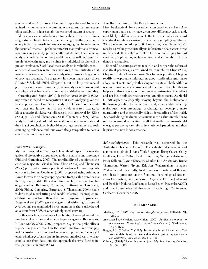
lations. First, consider a fictitious example and a picture (Fig. 1).

Volume 3—Number 4 287

Geoff Cumming

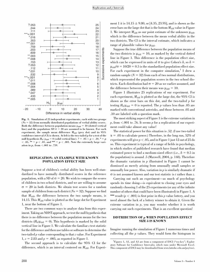
REPLICATION: AN EXAMPLE WITH KNOWNPOPULATION EFFECT SIZE

Suppose a test of children’s verbal ability has been well-stan-

dardized to have normally distributed scores in the reference

population, with a SD of s 5 20. We wish to compare the scores

of children in two school districts, and we are willing to assume

s 5 20 in both districts. We obtain test scores for a random

sample of children from each district (Ns 5 32). Suppose we find

that Mdiff, the difference between the two sample means, is

14.15. This Mdiff value is plotted as the large dot for Experiment

1, near the bottom of Figure 1.

There are two common ways to analyze data from this exper-

iment. Taking an NHSTapproach, we test the null hypothesis that

there is no difference between the population means for the two

districts (H0:mdiff 5 0). This hypothesis is marked by the solid

vertical line in Figure 1. We calculate the familiar z test statistic

for the difference and then use tables or software to determine the

two-tailed p value corresponding to that z value. For Experiment

1, z 5 2.83 and p 5 .005, as reported in Figure 1.

The second approach is to calculate the 95% CI for the

difference, which is an interval centered on Mdiff. For Experi-

ment 1 it is 14.15 � 9.80, or [4.35, 23.95], and is shown as the

error bars on the large dot that is the bottom Mdiff value in Figure

1. We interpret Mdiff as our point estimate of the unknown mdiff,

which is the difference between the mean verbal ability in the

two districts. The CI is the interval estimate, which indicates a

range of plausible values for mdiff.

Suppose the true difference between the population means of

the two districts is mdiff 5 10, as marked by the vertical dotted

line in Figure 1. This difference is the population effect size,

which can be expressed in units of s to give Cohen’s d, so d 5

mdiff/s 5 10/20 5 0.5 is the standardized population effect size.

For each experiment in the computer simulation,1 I drew a

random sample (N 5 32) from each of two normal distributions,

which represented the population scores in the two school dis-

tricts. Each distribution had s 5 20 as we earlier assumed, and

the difference between their means was mdiff 5 10.

Figure 1 illustrates 25 replications of our experiment. For

each experiment, Mdiff is plotted as the large dot, the 95% CI is

shown as the error bars on this dot, and the two-tailed p for

testing H0:mdiff 5 0 is reported. The p values less than .05 are

marked with conventional asterisks, and those between .05 and

.10 are labeled with a question mark.

The most striking aspect of Figure 1 is the extreme variation in

p, from <.001 to .76. It seems p for a replication of our experi-

ment could take almost any value!

The statistical power for this situation is .52. (I use two-tailed

a 5 .05 to calculate power.) Therefore, in the long run, 52% of

experiments will give p< .05, and in Figure 1 just 12 out of 25 do

so. This experiment is typical of a range of fields in psychology,

in which studies of published research have found that median

estimated power to find a medium-sized effect (i.e., d 5 0.5 in

the population) is around .5 (Maxwell, 2004, p. 148). Therefore

the dramatic variation in p illustrated in Figure 1 cannot be

dismissed as merely arising from unusually small samples or

unusually low power. Also, variation in p is similarly dramatic if

s is not assumed known and our test statistic is t rather than z.

Carrying out such an experiment—as much of psychology

spends its time doing—is equivalent to closing your eyes and

randomly choosing 1 of the 25 experiments (or any of the infinite

number of others that could have been illustrated) in Figure 1. Annn result (p < .001) is first prize in this p value lottery, and you

need almost the luck of a lottery winner to obtain it. Given the

extreme variation in p, you may wonder whether it is worth

carrying out such experiments. That is an excellent question!

DISTRIBUTION OF p WHEN POPULATION EFFECTSIZE d IS KNOWN

Imagine running the simulation of Figure 1 numerous times and

collecting all the p values. They would form the histogram in

.433

.389

.008

.031

.053

.008

.609

.759

.053

.244

.111

.016

.001

.203

.003

.153

.112

.532

.011

.004

.047

.005

.353

**

*

?

**

**

*

**

*

**

***

*

? 25242322212019181716151413121110987654321

−20

Difference in verbal ability

HS

ucce

ssiv

e ex

perim

ents

***<.001

***<.001

µ

−10 0 10 20 30 40

Fig. 1. Simulation of 25 independent experiments, each with two groups(Ns 5 32) from normally distributed populations of verbal ability scores.Both the difference between population means mdiff 5 10 (dotted verticalline) and the population SD s 5 20 are assumed to be known. For eachexperiment, the sample mean difference Mdiff (grey dot) and its 95%confidence interval (CI) is shown. At left is the two-tailed p for a test of thenull hypothesis H0: mdiff 5 0 (solid vertical line). ? 5 .05 < p < .10, n 5 p< .05, nn 5 p < .01, and nnn 5 p < .001. Note the extremely large vari-ation in p, from <.001 to .759.

1Figures 1, A1, and A3 are from a component of ESCI (‘‘ess-key’’; Explor-atory Software for Confidence Intervals), which runs under Microsoft Excel.This component of ESCI may be downloaded from www.latrobe.edu.au/psy/esci.

288 Volume 3—Number 4

Replication and p Intervals

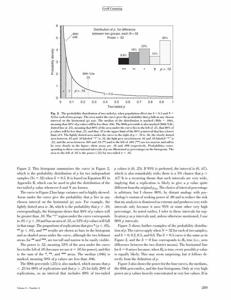
Figure 2. This histogram summarizes the curve in Figure 2,

which is the probability distribution of p for two independent

samples (Ns 5 32) when d 5 0.5. It is based on Equation B1 in

Appendix B, which can be used to plot the distribution of the

two-tailed p value whenever d and N are known.

The curve in Figure 2 has large variance and is highly skewed.

Areas under the curve give the probability that p lies in any

chosen interval on the horizontal (p) axis. For example, the

lightly dotted area is .36, which is the probability that p > .10;

correspondingly, the histogram shows that 36% of p values will

be greater than .10. The ‘‘?’’ region under the curve corresponds

to .05< p< .10 and has an area of .12, so 12% of p values will fall

in that range. The proportions of replications that give n ( p< .05),nn (p < .01), and nnn results are shown as bars in the histogram

and as shaded areas under the curve, although the two leftmost

areas, for nn and nnn, are too tall and narrow to be easily visible.

The power is .52, meaning 52% of the area under the curve

lies to the left of .05 (because we use a5 .05 for power), and this

is the sum of the n, nn, and nnn areas. The median (.046) is

marked, meaning 50% of p values are less than .046.

The 80th percentile (.25) is also marked, which means that p

< .25 for 80% of replications and that p > .25 for fully 20% of

replications, so an interval that includes 80% of two-tailed

p values is (0, .25). If 95% is preferred, the interval is (0, .67),

which is also remarkably wide; there is a 5% chance that p >

.67! It is a recurring theme that such intervals are very wide,

implying that a replication is likely to give a p value quite

different from the original pobt. The choice of interval percentage

is arbitrary, but I choose 80%, by distant analogy with psy-

chology’s custom of seeking power of .80 and to reduce the risk

that my analysis is dismissed as extreme and produces very wide

intervals only because it uses 95% or some other very high

percentage. As noted earlier, I refer to these intervals for rep-

lication p as p intervals and, unless otherwise mentioned, I use

80% p intervals.

Figure 3 shows further examples of the probability distribu-

tion of p. The curves apply when N 5 32 for each of two samples,

and d 5 0, 0.2, 0.5, and 0.8. The d 5 0.5 curve is the same as in

Figure 2, and the d 5 0 line corresponds to H0 true (i.e., zero

difference between the two district means). The horizontal line

for d 5 0 arises because, when H0 is true, every possible p value

is equally likely. This may seem surprising, but it follows di-

rectly from the definition of p.

Figure 3 also shows the power for the four curves, the medians,

the 80th percentiles, and the four histograms. Only at very high

power are p values heavily concentrated at very low values. If in

δ = 0.5* ? p > .10

80th %ile

Mdn.046

.25

0

1

2

3

4

5

6

0

Two-tailed p

Pro

babi

lity

dens

ity

Distribution of p , for difference between two groups, each N = 32

Power = .52 36%

12%

23%18%

9.8%

?****** p > .10

0.1 0.2 0.3 0.4 0.5 0.6 0.7 0.8 0.9 1

Fig. 2. The probability distribution of two-tailed p, when population effect size d 5 0.5 and N 5

32 for each of two groups. The area under the curve gives the probability that p falls in any choseninterval on the horizontal (p) axis. The median of the distribution is marked (Mdn 5 .046),meaning that 50% of p values will be less than .046. The 80th percentile is also marked (80th %ile;dotted line at .25), meaning that 80% of the area under the curve lies to the left of .25, that 80% ofp values will be less than .25, and that .25 is the upper limit of the 80% p interval that has a lowerlimit of 0. The lightly dotted area under the curve to the right of p 5 .10 is .36, the closely dottedarea between .05 and .10 labeled ‘‘?’’ is .12, the light grey area between .01 and .05 labeled ‘‘n’’ is.23, and the areas between .001 and .01 (nn) and to the left of .001 (nnn) are too narrow and tall tobe seen clearly in the figure—their areas are .18 and .098 respectively. Probabilities corre-sponding to these conventional intervals of p are illustrated as percentages in the histogram. Thearea to the left of .05 is the power (.52) for two-tailed a 5 .05.


Geoff Cumming

our example mdiff 5 16 and thus d 5 0.8—conventionally re-

garded as a large effect—then power is .89, which is a very high

value for psychology. Even then the p interval is (0, .018), so

fully 20% of p values will be greater than .018.

Distribution of p Depends Only on Power

Power determines the distribution of p, as Appendix B explains.

Power varies with N and population effect size d, and a partic-

ular value of power can reflect a number of pairs of N and dvalues. Any pair that gives that value of power will give the same

distribution of p. Thus, in the example, power is .52 for two

samples of N 5 32 when d 5 0.5. Power would also be .52 for

various other combinations of sample size and population effect

size: for example, N 5 8 and d5 1.0, or N 5 200 and d5 0.2, or

even N 5 800 and d 5 0.1. The distribution and histogram in

Figure 2 applies in all of those cases, because power is .52 for

each. Even for a very large N, if power is .52, the p interval will

still be (0, .25).

A curve and histogram like those in Figures 2 and 3 can be

calculated for any given power. Figure 4 shows in cumulative

form the percentages of the different ranges of p for a selection of

power values from .05 (i.e., d5 0, or H0 true) to .9. The values for

the bar representing a power of .5 are very similar to the per-

centages shown in Figure 2, in which power is .52. To help link

the distributions in Figure 4 back to my example, the corre-

sponding effect sizes (d values) when N 5 32 for each group are

shown at the right.

p Is a Poor Basis for Inference

Consider how uninformative p is for the true value of d. Noting

where p, calculated from data, falls along the horizontal axis in

Figure 3 does not give a clear indication as to which of the in-

finite family of curves—which of the possible d values—is likely

to be correct. Figure 4 also shows only a gradual change in

distributions with changes in power or effect size, again sug-

gesting p is very uninformative about d. Obtaining p 5 .05, for

example, gives very little hint as to which of the curves in Figure

3 or which of the d values in Figure 4 is the best bet to be the

cause of that particular p value.

Alternatively, we could focus not on estimating d, but only on

judging whether H0 is true; that is, whether d equals zero or not.

Figure 3 suggests that most p values do not provide a good basis

for choosing between the d 5 0 horizontal line and any other

curve. Figure 4 shows that p values greater than .01 or even .05

are quite common for medium to high power (the lower bars in

the figure), and that a minority of p values less than .01 do occur

for low to medium power (the upper bars). In other words, most

p values provide very poor guidance as to whether or not H0 is

true. This conclusion throws doubt on conventional practice in

which a p value is used to make sharp discriminations between

situations allowing rejection of H0 and those that do not. Onlynnn, and to a lesser extent nn, p values have much diagnostic

value about whether H0 is true. However, a result of nnn is often

sufficiently clear cut to hit you between the eyes, and so it is

hardly a triumph for p that it rejects a hypothesis of zero effect in

such cases!

In summary, the distribution of two-tailed p when the power is

known or when d and N are known is illustrated in Figures 2 and

3. The distribution is highly skewed (unless d 5 0) and is in-

dependent of N for a given power. It generally has large variance,

and the p intervals are very wide. Figures 3 and 4 suggest only

very small p values have much diagnostic value as to whether or

not the true effect size is zero.

δ=0.2δ=0.5δ=0.8

δ=0

0

1

2

3

4

5

6

0 0.1 0.2 0.3 0.4 0.5 0.6 0.7 0.8 0.9 1

Two-tailed p

Pro

babi

lity

dens

ityDistributions of p , for difference between two groups, each N =32

Fig. 3. Probability distributions of p for two groups (Ns 5 32) when d 5

0 (i.e., H0 true) and d 5 0.2, 0.5, and 0.8, which can be regarded as small,medium and large effects, respectively. The d 5 0.5 curve is the same asthat in Figure 2. For each value of d, the power, median (Mdn), and 80thpercentile (80th %ile) are tabulated and the histogram of p values isshown; the 80th percentile is the upper limit of the p interval with a lowerlimit of 0. ? 5 .05< p< .10, n 5 p< .05, nn 5 p< .01, and nnn 5 p< .001.

Two-tailed p

******

******

****

****

****

**

*

**

**

?

?

?******

**

**

**

*

?

?

?

?

?

?

?

p >.10

p >.10

p >.10

p >.10

p >.10

p >.10

p >.10

p >.10

0% 10% 20% 30% 40% 50% 60% 70% 80% 90%

.05

.1

.2

.3

.4

.5

.6

.7

.8

.9

Po

we

r

Cumulative frequency

δ 0

.16

.28

.36

.43

.49

.55

.62

.70

.81

100%

If two groups, N=32:

Fig. 4. Cumulative frequencies for p, for different values of power.When H0 is true (the top bar), the power is .05 and the shaded bars show acumulated 5% chance of p in the three ranges marked by asterisks(<.001; .001–.01; .01–.05, respectively) and a further 5% chance that .05< p < .10. The percentages for .5 power are very similar to those in thehistogram in Figure 2, in which the power is .52. For a given power, thepercentages are independent of N. If N 5 32 for each of two groups, thecorresponding d values are shown at right.



DISTRIBUTION OF p GIVEN ONLY AN INITIAL pobt

The initial example above was based on the unrealistic as-

sumption that we know d, the size of the effect in the population,

and the distributions in Figures 2–4 relied on knowing d and N,

or power. I now assume that d is not known and consider the

distribution of the p value after an initial experiment has yielded

Mdiff, from which the pobt is calculated. The appendices explain

how the probability distribution of p can be derived without

knowing or assuming a value for d (or power). The basic idea is

that our initial Mdiff is assumed to come from populations with

some unknown effect size d. Our Mdiff does not give a precise

value for d, but does give sufficient information about it for us to

find a distribution for replication p values, given only pobt from

the initial experiment. We do not assume any prior knowledge

about d, and we use only the information Mdiff gives about d as

the basis for the calculation for a given pobt of the distribution of

p and of p intervals.

I have set my whole argument, including the derivation of

p intervals without assuming a value for d, in a conventional

frequentist framework because that is most familiar to most

psychologists. However, an alternative approach within a

Bayesian framework is appealing, although it is important to

recognize that the two conceptual frameworks are quite different

and license different interpretive wording of conclusions.

Even so, they sometimes give the same numerical results. For

example in some simple situations, using reasonable assump-

tions, the 95% CI is numerically the same as the Bayesian 95%

credible interval. A researcher can regard the interval as a

pragmatically useful indication of uncertainty, without neces-

sarily being concerned with the niceties of the interpretation

permitted by either framework. Similarly, when finding p inter-

vals without assuming a value for d, a Bayesian analysis would

start with a prior probability distribution that expresses our ig-

norance of d. Then, as an anonymous reviewer pointed out, it

could give formulas for p intervals that are the same as mine, but

with different underlying conceptualizations. Therefore, p in-

tervals indicate the vagueness of the information given by p, no

matter which conceptual framework is preferred.

So far all p values have been two-tailed. I based the first

discussion on two-tailed p because of its familiarity. However,

even using two-tailed pobt, it is more natural to consider one-

tailed p values given by replications (replication one-tailed p),

because the initial experiment indicates a direction for the ef-

fect—although of course this could be wrong. From here on

I will, unless otherwise stated, use two-tailed pobt and replication

one-tailed p.

The probability distribution of replication p, for any chosen

value of pobt, can be plotted by use of Equation B3 in Appendix

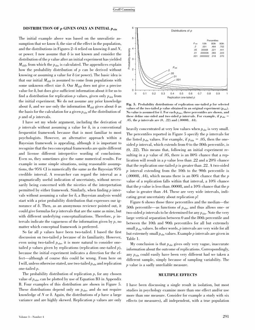
B. Four examples of this distribution are shown in Figure 5.

These distributions depend only on pobt, and do not require

knowledge of N or d. Again, the distributions of p have a large

variance and are highly skewed. Replication p values are only

heavily concentrated at very low values when pobt is very small.

The percentiles reported in Figure 5 specify the p intervals for

the listed pobt values. For example, if pobt 5 .05, then the one-

sided p interval, which extends from 0 to the 80th percentile, is

(0, .22). This means that, following an initial experiment re-

sulting in a p value of .05, there is an 80% chance that a rep-

lication will result in a p value less than .22 and a 20% chance

that the replication one-tailed p is greater than .22. A two-sided

p interval extending from the 10th to the 90th percentile is

(.00008, .44), which means there is an 80% chance that the p

value of a replication falls within that interval, a 10% chance

that the p value is less than .00008, and a 10% chance that the p

value is greater than .44. These are very wide intervals, indi-

cating great uncertainty about replication p!

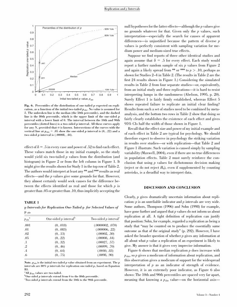
Figure 6 shows those three percentiles and the median—the

50th percentile—as functions of pobt, and thus allows one- or

two-sided p intervals to be determined for any pobt. Note the very

large vertical separation between 0 and the 80th percentile and

between the 10th and 90th percentiles for all but extremely

small pobt values. In other words, p intervals are very wide for all

but extremely small pobt values. Example p intervals are given in

Table 1.

My conclusion is that pobt gives only very vague, inaccurate

information about the outcome of replications. Correspondingly,

any pobt could easily have been very different had we taken a

different sample, simply because of sampling variability. The

p value is a sadly unreliable measure.

MULTIPLE EFFECTS

I have been discussing a single result in isolation, but most

studies in psychology examine more than one effect and/or use

more than one measure. Consider for example a study with six

effects (or measures), all independent, with a true population

.001.01

.05.2

p

0

1

2

3

4

5

6

0 0.1 0.2 0.3 0.4 0.5 0.6 0.7 0.8 0.9 1

Replication one-tailed p

Pro

babi

lity

dens

ity

Distributions of p

Fig. 5. Probability distributions of replication one-tailed p for selectedvalues of the two-tailed p value obtained in an original experiment (pobt).No value is assumed for d. For each pobt, three percentiles are shown, andthese define one-sided and two-sided p intervals. For example, if pobt 5

.05, the p intervals are (0, .22) and (.00008, .44).


Geoff Cumming

effect of d5 .5 in every case and power of .52 to find each effect.

These values match those in my initial example, so the study

would yield six two-tailed p values from the distribution (and

histogram) in Figure 2 or from the left column in Figure 1. It

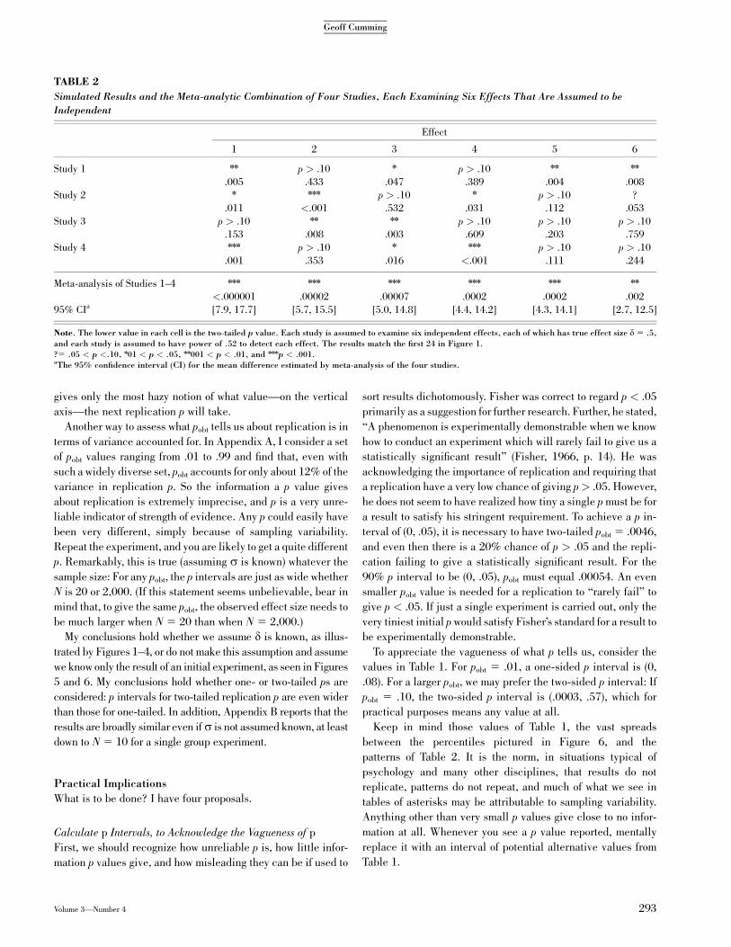
might give the results shown for Study 1 in the top row of Table 2.

The authors would interpret at least any nn and nnn results as real

effects—and the p values give some grounds for that. However,

they almost certainly would seek causes for the difference be-

tween the effects identified as real and those for which p is

greater than .05 or greater than .10, thus implicitly accepting the

null hypotheses for the latter effects—although the p values give

no grounds whatever for that. Given only the p values, such

interpretation—especially the search for causes of apparent

differences—is unjustified because the pattern of diverse p

values is perfectly consistent with sampling variation for me-

dium power and medium-sized true effects.

Suppose we find reports of three other identical studies and

again assume that d 5 .5 for every effect. Each study would

report a further random sample of six p values from Figure 2

and again a likely spread from nn or nnn to p > .10, perhaps as

shown for Studies 2–4 in Table 2. (The results in Table 2 are the

first 24 results shown in Figure 1.) Considering the simulated

results in Table 2 from four separate studies—or, equivalently,

from an initial study and three replications—it is hard to resist

interpreting lumps in the randomness (Abelson, 1995, p. 20).

Surely Effect 1 is fairly firmly established, whereas Effect 5

shows repeated failure to replicate an initial clear finding?

Results from such a set of studies need to be combined by meta-

analysis, and the bottom two rows in Table 2 show that doing so

fairly clearly establishes the existence of each effect and gives

95% CIs half the width of those shown in Figure 1.

Recall that the effect size and power of my initial example and

of each effect in Table 2 are typical for psychology. We should

therefore expect to observe in psychology the striking variation

in results over studies—or with replication—that Table 2 and

Figure 1 illustrate. Such variation is caused simply by sampling

variability (Maxwell, 2004), even if there are no true differences

in population effects. Table 2 must surely reinforce the con-

clusion that using p values for dichotomous decision making

(reject or do not reject H0), even if supplemented by counting

asterisks, is a dreadful way to interpret data.

DISCUSSION AND CONCLUSION

Clearly, p gives dramatically uncertain information about repli-

cation: p is an unreliable indicator and p intervals are very wide.

Some authors, Thompson (1996) and Sohn (1998) for example,

have gone further and argued that p values do not inform us about

replication at all. A tight definition of replication can justify

that position: Sohn, for example, regarded a replication as being a

study that ‘‘may be counted on to produce the essentially same

outcome as that of the original study’’ (p. 292). However, I have

asked the broader question of whether p gives any information at

all about what p value a replication of an experiment is likely to

give. My answer is that it gives very imprecise information.

Figure 6 shows that median replication p does increase with

pobt, so p gives a modicum of information about replication, and

this observation gives a modicum of support for the widespread

interpretation of p as an indicator of strength of evidence.

However, it is an extremely poor indicator, as Figure 6 also

shows: The 10th and 90th percentiles are spaced very far apart,

meaning that knowing a pobt value—on the horizontal axis—

0

0.1

0.2

0.3

0.4

0.5

0.6

0.7

0.8

0.9

1

0 0.1 0.2 0.3 0.4 0.5 0.6 0.7 0.8 0.9 1

Initial two-tailed p value, p

Rep

licat

ion

one-

taile

d p

val

uePercentiles of the distribution of p

Fig. 6. Percentiles of the distribution of one-tailed p expected on repli-cation, as a function of the initial two-tailed pobt. No value is assumed ford. The unbroken line is the median (the 50th percentile), and the dashedline is the 80th percentile, which is the upper limit of the one-sided pinterval with a lower limit of 0. The interval between the 10th and 90thpercentiles (dotted lines) is a two-sided p interval. All these curves applyfor any N, provided that s is known. Intersections of the curves with thevertical line at pobt 5 .05 show the one-sided p interval is (0, .22) and atwo-sided p interval is (.00008, .44).

TABLE 1

p Intervals for Replication One-Tailed p for Selected Values of

p obt

pobta One-sided p intervalb Two-sided p intervalc

.001 (0, .018) (.0000002, .070)

.01 (0, .083) (.000006, .22)

.02 (0, .13) (.00002, .30)

.05 (0, .22) (.00008, .44)

.1 (0, .32) (.00027, .57)

.2 (0, .46) (.00099, .70)

.4 (0, .64) (.0040, .83)

.6 (0, .75) (.0098, .90)

Note. pobt is the initial two-tailed p value obtained from an experiment. The pintervals are 80% p intervals for replication one-tailed p, based on EquationB3.aAll pobt values are two-tailed.bOne-sided p intervals extend from 0 to the 80th percentile.cTwo-sided p intervals extend from the 10th to the 90th percentile.



gives only the most hazy notion of what value—on the vertical

axis—the next replication p will take.

Another way to assess what pobt tells us about replication is in

terms of variance accounted for. In Appendix A, I consider a set

of pobt values ranging from .01 to .99 and find that, even with

such a widely diverse set, pobt accounts for only about 12% of the

variance in replication p. So the information a p value gives

about replication is extremely imprecise, and p is a very unre-

liable indicator of strength of evidence. Any p could easily have

been very different, simply because of sampling variability.

Repeat the experiment, and you are likely to get a quite different

p. Remarkably, this is true (assuming s is known) whatever the

sample size: For any pobt, the p intervals are just as wide whether

N is 20 or 2,000. (If this statement seems unbelievable, bear in

mind that, to give the same pobt, the observed effect size needs to

be much larger when N 5 20 than when N 5 2,000.)

My conclusions hold whether we assume d is known, as illus-

trated by Figures 1–4, or do not make this assumption and assume

we know only the result of an initial experiment, as seen in Figures

5 and 6. My conclusions hold whether one- or two-tailed ps are

considered: p intervals for two-tailed replication p are even wider

than those for one-tailed. In addition, Appendix B reports that the

results are broadly similar even ifs is not assumed known, at least

down to N 5 10 for a single group experiment.

Practical Implications

What is to be done? I have four proposals.

Calculate p Intervals, to Acknowledge the Vagueness of p

First, we should recognize how unreliable p is, how little infor-

mation p values give, and how misleading they can be if used to

sort results dichotomously. Fisher was correct to regard p < .05

primarily as a suggestion for further research. Further, he stated,

‘‘A phenomenon is experimentally demonstrable when we know

how to conduct an experiment which will rarely fail to give us a

statistically significant result’’ (Fisher, 1966, p. 14). He was

acknowledging the importance of replication and requiring that

a replication have a very low chance of giving p> .05. However,

he does not seem to have realized how tiny a single p must be for

a result to satisfy his stringent requirement. To achieve a p in-

terval of (0, .05), it is necessary to have two-tailed pobt 5 .0046,

and even then there is a 20% chance of p > .05 and the repli-

cation failing to give a statistically significant result. For the

90% p interval to be (0, .05), pobt must equal .00054. An even

smaller pobt value is needed for a replication to ‘‘rarely fail’’ to

give p < .05. If just a single experiment is carried out, only the

very tiniest initial p would satisfy Fisher’s standard for a result to

be experimentally demonstrable.

To appreciate the vagueness of what p tells us, consider the

values in Table 1. For pobt 5 .01, a one-sided p interval is (0,

.08). For a larger pobt, we may prefer the two-sided p interval: If

pobt 5 .10, the two-sided p interval is (.0003, .57), which for

practical purposes means any value at all.

Keep in mind those values of Table 1, the vast spreads

between the percentiles pictured in Figure 6, and the

patterns of Table 2. It is the norm, in situations typical of

psychology and many other disciplines, that results do not

replicate, patterns do not repeat, and much of what we see in

tables of asterisks may be attributable to sampling variability.

Anything other than very small p values give close to no infor-

mation at all. Whenever you see a p value reported, mentally

replace it with an interval of potential alternative values from

Table 1.

TABLE 2

Simulated Results and the Meta-analytic Combination of Four Studies, Each Examining Six Effects That Are Assumed to be

Independent

Effect

1 2 3 4 5 6

Study 1 nn p > .10 n p > .10 nn nn

.005 .433 .047 .389 .004 .008

Study 2 n nnn p > .10 n p > .10 ?

.011 <.001 .532 .031 .112 .053

Study 3 p > .10 nn nn p > .10 p > .10 p > .10

.153 .008 .003 .609 .203 .759

Study 4 nnn p > .10 n nnn p > .10 p > .10

.001 .353 .016 <.001 .111 .244

Meta-analysis of Studies 1–4 nnn nnn nnn nnn nnn nn

<.000001 .00002 .00007 .0002 .0002 .002

95% CIa [7.9, 17.7] [5.7, 15.5] [5.0, 14.8] [4.4, 14.2] [4.3, 14.1] [2.7, 12.5]

Note. The lower value in each cell is the two-tailed p value. Each study is assumed to examine six independent effects, each of which has true effect size d 5 .5,and each study is assumed to have power of .52 to detect each effect. The results match the first 24 in Figure 1.?5 .05 < p <.10, n01 < p < .05, nn001 < p < .01, and nnnp < .001.aThe 95% confidence interval (CI) for the mean difference estimated by meta-analysis of the four studies.


Geoff Cumming

Rosenthal and Gaito (1963, 1964) presented evidence that

psychologists show a cliff effect, meaning that small differences

in p near .05 give fairly sharp differences in confidence that an

effect exists. My analyses give further reasons why such beliefs

are unjustified. Rosnow and Rosenthal (1989) famously stated

‘‘Surely, God loves the .06 nearly as much as the .05’’ (p. 1277),

to which we can now reply ‘‘Yes, but God doesn’t love either of

them very much at all, because they convey so little!’’ The se-

ductive certainty touted by p values may be one of the more

dramatic and pernicious manifestations of the ironically named

Law of Small Numbers (Tversky & Kahneman, 1971), which is

the misconception that even small samples give accurate in-

formation about their parent populations.

Psychologists have expended vast effort to develop sophisti-

cated statistical methods to minutely adjust p value calculations

to avoid various biases in particular situations, while remaining

largely blind to the fact that the p value being precisely tweaked

could easily have been very different. You are unlikely to be

anxious to calculate p 5 .050 so exactly if you know the p in-

terval is (.00008, .44)!

In many disciplines it is customary to report a measurement

as, for example, 17.43� .02 to indicate precision. By analogy, if

a p value is to be reported, journals should also require reporting

of the p interval to indicate the level of vagueness or unreli-

ability. Having to report a test of statistical significance as ‘‘z 5

2.05, p 5 .04, p interval (0, .19)’’ may be the strongest motivator

for psychologists to find better ways to draw inferences from

data.

Use CIs

The American Psychological Association (APA) Publication

Manual (APA, 2001, p. 22) strongly recommends the use of CIs.

Many advocates of statistical reform, including Kline (2004,

Chapter 3) and Cumming and Finch (2005), have presented

reasons why psychologists should use CIs wherever possible. My

discussion of replication identifies a further advantage of CIs.

Consider Figure 1 again. Following a single experiment, would

you prefer to be told only the p value (and perhaps Mdiff) or would

you prefer to see the CI? Is a single p value representative of the

infinite set of possible results? Is it a reasonable exemplar of the

whole set? Hardly! I suggest a single CI is more representative, a

better exemplar, and can give a better sense of the whole set,

including the inherent uncertainty. A p value gives only vague

information about what is likely to happen next time, but doesn’t

a CI give more insight?

In other words, CIs give useful information about replication.

More specifically, any CI is also a prediction interval: The

probability is .83 that the mean of a replication will fall within a

95% CI (Cumming & Maillardet, 2006; Cumming et al., 2004),

so CIs give direct information about replication. In Figure 1, in

17 of 24 cases, the pictured 95% CI includes the mean of the

next experiment; in the long run, 83% of the CIs will include the

next mean. A 95% CI is not only an interval estimate for mdiff, it is

also an 83% prediction interval for where the next Mdiff will fall.

Think Meta-Analytically

A possible response to my findings is to continue using NHST

but acknowledge the message of Figure 4—which is that only nnn

(and perhaps nn) results are very clearly diagnostic of an effect—

and by adopting a small a and, for example, rejecting the null

hypothesis only when p is less than .01 or even less than .001.

The problem, however, is that even with the dreamworld power of

.9 there is a 25% chance of not obtaining p < .01. Therefore, at

the less-than-ideal power psychologists typically achieve, ob-

taining nn or nnn results requires luck, which implies there is

much unlucky research effort that is wasted. It is worse than

wasted because, as meta-analysts make clear (Schmidt, 1996), if

asterisks influence publication, then estimates of effect sizes

based on published evidence are inflated.

It is a worthy goal to conduct high-powered studies. Investi-

gate large effects if you can, raise large grants so you can afford

to use large samples, and use every other strategy to increase

power (Maxwell, 2004). Finding effects that pass the interocular

trauma test—that hit you between the eyes—largely sidesteps

the problems of statistical inference.

However, as we have seen, not even high power guarantees

that a single experiment will give a definitive result. In the words

of the APA Task Force on Statistical Inference: ‘‘The results in a

single study are important primarily as one contribution to a

mosaic of study effects’’ (Wilkinson & Task Force on Statistical

Inference, 1999, p. 602). There is usually more error variability

inherent in any single result than we realize. A CI makes that

uncertainty salient—that is why CIs in psychology are often

depressingly wide. By contrast, a p value papers over the in-

herent uncertainty by tempting us to make a binary decision,

which can easily mislead us to believe that little doubt remains.

The uncertainty in single results implies that evidence needs

to be combined over experiments. Recognizing the central role

of replication for scientific progress also emphasizes the need to

combine evidence over experiments, and meta-analysis is the

way to do this quantitatively. Meta-analysis applied to the four

experiments in Table 2 establishes each effect virtually con-

clusively and gives reasonably precise estimates of each. On this

large scale of combining evidence from different studies, meta-

analysis provides the best foundation for progress, even for

messy applied questions. When high power is not feasible, meta-

analysis of a number of studies is especially necessary.

Reports surface from time to time, from any of a range of

disciplines, of difficulty in replicating published findings. In

medicine, for example, recent discussion (Ioannidis, 2005) has

identified many cases of apparently clear results being ques-

tioned after attempts at replication. Selective and biased re-

porting of single results may play a role, but the surprising extent

of sampling variability, as illustrated in Table 2, may be a

primary contributor to any surprising disagreement between



similar studies. Any cases of failure to replicate need to be ex-

amined by meta-analysis to determine the extent that mere sam-

pling variability might explain the observed pattern of results.

Meta-analysis can also be used to combine evidence within a

single study. The astute experimenter recognizes the uncertainty

of any individual result and seeks converging results relevant to

the issue of interest—perhaps different manipulations or mea-

sures in a single study, perhaps different studies. Then, a meta-

analytic combination of comparable results will increase the

precision of estimates, and p values for individual results will be

proven irrelevant. Such local meta-analysis is valuable even—

or especially—for research in a new area, thus illustrating that

meta-analysis can contribute not only when there is a large body

of previous research. The argument has been made many times

(Hunter & Schmidt, 2004, Chapter 1), but the large variance of

p provides one more reason why meta-analysis is so important

and why it is the best route to truth in a world of error variability.

Cumming and Finch (2001) described meta-analytic think-

ing, which is based on recognition that meta-analysis gives the

best appreciation of one’s own study in relation to other stud-

ies—past and future—and to the whole research literature.

Meta-analytic thinking was discussed with approval by Kline

(2004, p. 12) and Thompson (2006, Chapters 7 & 9). Meta-

analytic thinking should influence all consideration of data and

drawing of conclusions. It should encourage researchers to seek

converging evidence and thus avoid the p temptation to base a

conclusion on a single result.

Find Better Techniques

My final proposal is that psychology should speed its investi-

gation of alternative approaches to data analysis and inference

(Fidler & Cumming, 2007). The unreliability of p reinforces the

case for major statistical reform. Kline (2004) and Thompson

(2006) provided extensive practical guidance for how psychol-

ogy can do better. Goodman (2001) proposed using minimum

Bayes factors as an easy stepping stone from p value practices to

the Bayesian world. Other disciplines such as conservation bi-

ology (Fidler, Burgman, Cumming, Buttrose, & Thomason,

2006; Fidler, Cumming, Burgman, & Thomason, 2004) make

wider use of model-fitting and model-selection techniques in-

cluding information theoretic and Bayesian approaches.

Wagenmakers (2007) gave a cogent and withering critique of

p values and recommended Bayesian methods that can be based

on output from SPSS or other widely used software.

In this article, my analysis of replication has emphasized the

problems of p values and thus is largely negative. By contrast,

Killeen (2005, 2006, 2007) proposed prep as the probability a

replication gives a result in the same direction, and thus prep

makes positive use of information about replication. It is not yet

clear whether prep can support improved practical ways to draw

conclusions from data, but the approach deserves further in-

vestigation (Cumming, 2005).

The Bottom Line for the Busy Researcher

First, be skeptical about any conclusion based on p values. Any

experiment could easily have given very different p values and,

most likely, a different pattern of effects—especially in terms of

statistical significance—simply because of sampling variability.

With the exception of a p < .001 result (or, possibly, a p < .01

result), a p value gives virtually no information about what is true

in the world. It is better to think in terms of converging lines of

evidence, replication, meta-analysis, and cumulation of evi-

dence over studies.

Second, I encourage others to join in and support the reform of

statistical practices, as explained for example by Kline (2004,

Chapter 3). As a first step, use CIs wherever possible. CIs give

readily interpretable information about replication and make

adoption of meta-analytic thinking more natural, both within a

research program and across a whole field of research. CIs can

help us to think about point and interval estimates of an effect

and not focus only on whether or not an effect exists. As Meehl

(1978) argued so cogently, moving beyond the dichotomous

thinking of p values to estimation—and, we can add, modeling

techniques—can encourage psychology to develop a more

quantitative and theoretically rich understanding of the world.

Acknowledging the dramatic vagueness of p values in relation to

replication—and replication is all that really matters—should

energize psychology to reform its statistical practices and thus

improve the way it does science.

Acknowledgments—This research was supported by the

Australian Research Council. For valuable discussions and

comments on drafts, I thank Mark Burgman, Barry Cohen, Cathy

Faulkner, Fiona Fidler, Keith Hutchison, George Kahrimanis,

Peter Killeen, Glynda Kinsella, Charles Liu, Art Stukas, Bruce

Thompson, Warren Tryon, Eric-Jan Wagenmakers, Eleanor

Wertheim and, especially, Neil Thomason. Portions of this re-

search were presented at the American Psychological Associ-

ation Convention, San Francisco, August 2007; the Judgment

and Decision Making Conference, Long Beach, November 2007;

and the Australasian Mathematical Psychology Conference,

Canberra, December 2007.

REFERENCES

Abelson, R.P. (1995). Statistics as principled argument. Hillsdale, NJ:

Erlbaum.

American Psychological Association. (2001). Publication manual ofthe American Psychological Association (5th ed.). Washington,

DC: Author.

Berger, J.O., & Sellke, T. (1987). Testing a point null hypothesis: The

irreconcilability of p values and evidence. Journal of the Ameri-can Statistical Association, 82, 112–122.

Cohen, J. (1994). The earth is round (p < .05). American Psychologist,49, 997–1003.


Geoff Cumming

Cumming, G. (2005). Understanding the average probability of repli-

cation: Comment on Killeen (2005). Psychological Science, 16,

1002–1004.

Cumming, G. (2007). Inference by eye: Pictures of confidence intervals

and thinking about levels of confidence. Teaching Statistics, 29,

89–93.

Cumming, G., Fidler, F., Leonard, M., Kalinowski, P., Christiansen, A.,

Kleinig, A., et al. (2007). Statistical reform in psychology: Is

anything changing? Psychological Science, 18, 230–232.

Cumming, G., & Finch, S. (2001). A primer on the understanding, use,

and calculation of confidence intervals that are based on central

and noncentral distributions. Educational and Psychological

Measurement, 61, 530–572.

Cumming, G., & Finch, S. (2005). Inference by eye: Confidence in-

tervals and how to read pictures of data. American Psychologist,

60, 170–180.

Cumming, G., & Maillardet, R. (2006). Confidence intervals and

replication: Where will the next mean fall? Psychological Meth-

ods, 11, 217–227.

Cumming, G., Williams, J., & Fidler, F. (2004). Replication, and re-

searchers’ understanding of confidence intervals and standard

error bars. Understanding Statistics, 3, 299–311.

Dixon, P. (1998). Why scientists value p values. Psychonomic Bulletin

& Review, 5, 390–396.

Estes, W.K. (1997). On the communication of information by displays

of standard errors and confidence intervals. Psychonomic Bulletin

& Review, 4, 330–341.

Fidler, F., Burgman, M., Cumming, G., Buttrose, R., & Thomason, N.

(2006). Impact of criticisms of null-hypothesis significance test-

ing on statistical reporting practices in conservation biology.

Conservation Biology, 20, 1539–1544.

Fidler, F., & Cumming, G. (2007). The new stats: Attitudes for

the twenty-first century. In J.W. Osborne (Ed.), Best practices in

quantitative methods (pp. 1–12). Thousand Oaks, CA: Sage.

Fidler, F., Cumming, G., Burgman, M., & Thomason, N. (2004). Sta-

tistical reform in medicine, psychology and ecology. Journal of

Socio-Economics, 33, 615–630.

Fisher, R.A. (1959). Statistical methods and scientific inference (2nd

ed.). Edinburgh, United Kingdom: Oliver and Boyd.

Fisher, R.A. (1966). The design of experiments (8th ed.). Edinburgh,

United Kingdom: Oliver & Boyd.

Gigerenzer, G. (2004). Mindless statistics. Journal of Socio-Economics,

33, 587–606.

Goodman, S.N. (1992). A comment on replication, p-values and evi-

dence. Statistics in Medicine, 11, 875–879.

Goodman, S.N. (2001). Of p-values and Bayes: A modest proposal.

Epidemiology, 12, 295–297.

Goodman, S.N., & Royall, R. (1988). Evidence and scientific research.

American Journal of Public Health, 78, 1568–1574.

Greenwald, A.G., Gonzalez, R., Harris, R.J., & Guthrie, D. (1996).

Effect sizes and p values: What should be reported and what

should be replicated? Psychophysiology, 33, 175–183.

Haller, H., & Krauss, S. (2002). Misinterpretations of significance: A

problem students share with their teachers? Methods of Psycho-

logical Research, 7, 1–20.

Hubbard, R. (2004). Alphabet soup. Blurring the distinction between

ps and as in psychological research. Theory & Psychology, 14,

295–327.

Hung, H.M.J., O’Neill, R.T., Bauer, P., & Kohne, K. (1997). The be-

haviour of the p-value when the alternative hypothesis is true.

Biometrics, 53, 11–22.

Hunter, J.E., & Schmidt, F.L. (2004). Methods of meta-analysis. Cor-

recting error and bias in research findings (2nd ed.). Thousand

Oaks, CA: Sage.

Ioannidis, J. (2005). Contradicted and initially stronger effects in

highly cited clinical research. Journal of the American Medical

Association, 294, 218–228.

Kahrimanis, G., & Berleant, D. (2007). Direct pivotal predictive infer-

ence: I. The case of additive noise. Unpublished manuscript.

Killeen, P.R. (2005). An alternative to null hypothesis significance

tests. Psychological Science, 16, 345–353.

Killeen, P.R. (2006). Beyond statistical inference: A decision theory

for science. Psychonomic Bulletin & Review, 13, 549–562.

Killeen, P.R. (2007). Replication statistics. In J.W. Osborne (Ed.), Best

practices in quantitative methods (pp. 103–124). Thousand Oaks,

CA: Sage.

Kline, R.B. (2004). Beyond significance testing: Reforming data

analysis methods in behavioral research. Washington, DC:

American Psychological Association.

Maxwell, S.E. (2004). The persistence of underpowered studies in

psychological research: Causes, consequences, and remedies.

Psychological Methods, 9, 147–163.

Meehl, P.E. (1978). Theoretical risks and tabular asterisks: Sir Karl,

Sir Ronald, and the slow progress of soft psychology. Journal of

Consulting and Clinical Psychology, 46, 806–834.

Morgenthaler, S., & Staudte, R.G. (2007). Interpreting significant

p-values. Manuscript submitted for publication.

Mulkay, M., & Gilbert, G.N. (1986). Replication and mere replication.

Philosophy of the Social Sciences, 16, 21–37.

Oakes, M. (1986). Statistical inference: A commentary for the social and

behavioural sciences. Chichester, United Kingdom: Wiley.

Posavac, E.J. (2002). Using p values to estimate the probability of a

statistically significant replication. Understanding Statistics, 1,

101–112.

Rosenthal, R., & Gaito, J. (1963). The interpretation of levels of sig-

nificance by psychological researchers. Journal of Psychology,

55, 33–38.

Rosenthal, R., & Gaito, J. (1964). Further evidence for the cliff effect

in the interpretation of levels of significance. Psychological Re-

ports, 15, 570.

Rosnow, R.L., & Rosenthal, R. (1989). Statistical procedures and the

justification of knowledge in psychological science. American

Psychologist, 44, 1276–1284.

Sackrowitz, H., & Samuel-Cahn, E. (1999). p values as random

variables—expected p values. American Statistician, 53, 326–

331.

Schmidt, F.L. (1996). Statistical significance testing and cumulative

knowledge in psychology: Implications for training of research-

ers. Psychological Methods, 1, 115–129.

Sohn, D. (1998). Statistical significance and replicability: Why the

former does not presage the latter. Theory & Psychology, 8, 291–

311.

Thompson, B. (1996). AERA editorial policies regarding statistical

significance testing: Three suggested reforms. Educational Re-

searcher, 25, 26–30.

Thompson, B. (2006). Foundations of behavioral statistics: An insight-

based approach. New York: Guilford.

Tversky, A., & Kahneman, D. (1971). Belief in the law of small

numbers. Psychological Bulletin, 92, 105–110.

Wagenmakers, E.-J. (2007). A practical solution to the pervasive

problems of p-values. Psychonomic Bulletin & Review, 14, 779–

804.



Wilkinson, L. & Task Force on Statistical Inference. (1999). Statistical

methods in psychology journals: Guidelines and explanations.

American Psychologist, 54, 594–604.

APPENDIX A

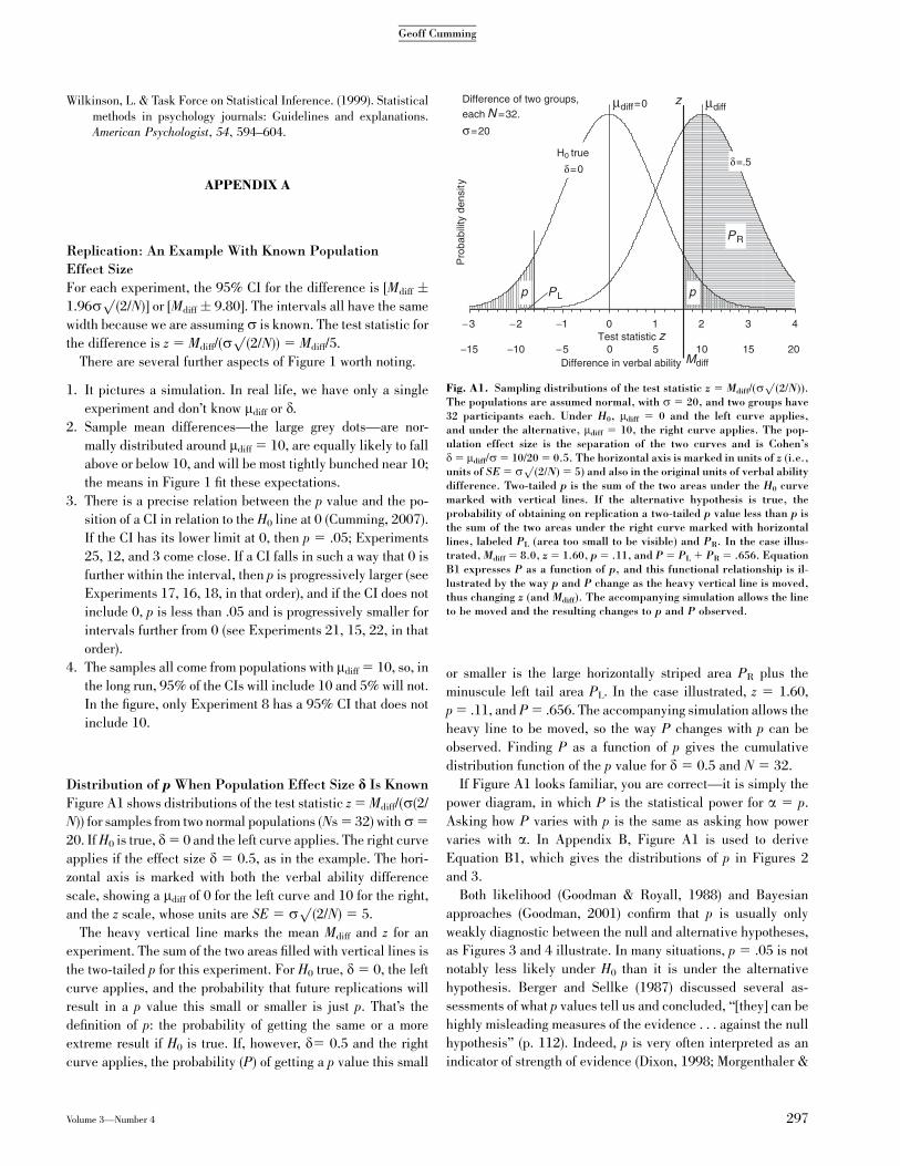
Replication: An Example With Known Population

Effect Size

For each experiment, the 95% CI for the difference is [Mdiff �1.96s

p(2/N)] or [Mdiff� 9.80]. The intervals all have the same

width because we are assuming s is known. The test statistic for

the difference is z 5 Mdiff/(sp

(2/N)) 5 Mdiff/5.

There are several further aspects of Figure 1 worth noting.

1. It pictures a simulation. In real life, we have only a single

experiment and don’t know mdiff or d.

2. Sample mean differences—the large grey dots—are nor-

mally distributed around mdiff 5 10, are equally likely to fall

above or below 10, and will be most tightly bunched near 10;

the means in Figure 1 fit these expectations.

3. There is a precise relation between the p value and the po-

sition of a CI in relation to the H0 line at 0 (Cumming, 2007).

If the CI has its lower limit at 0, then p 5 .05; Experiments

25, 12, and 3 come close. If a CI falls in such a way that 0 is

further within the interval, then p is progressively larger (see

Experiments 17, 16, 18, in that order), and if the CI does not

include 0, p is less than .05 and is progressively smaller for

intervals further from 0 (see Experiments 21, 15, 22, in that

order).

4. The samples all come from populations with mdiff 5 10, so, in

the long run, 95% of the CIs will include 10 and 5% will not.

In the figure, only Experiment 8 has a 95% CI that does not

include 10.

Distribution of p When Population Effect Size d Is Known

Figure A1 shows distributions of the test statistic z 5 Mdiff/(s(2/

N)) for samples from two normal populations (Ns 5 32) withs5

20. If H0 is true, d5 0 and the left curve applies. The right curve

applies if the effect size d 5 0.5, as in the example. The hori-

zontal axis is marked with both the verbal ability difference

scale, showing a mdiff of 0 for the left curve and 10 for the right,

and the z scale, whose units are SE 5 sp

(2/N) 5 5.

The heavy vertical line marks the mean Mdiff and z for an

experiment. The sum of the two areas filled with vertical lines is

the two-tailed p for this experiment. For H0 true, d 5 0, the left

curve applies, and the probability that future replications will

result in a p value this small or smaller is just p. That’s the

definition of p: the probability of getting the same or a more

extreme result if H0 is true. If, however, d5 0.5 and the right

curve applies, the probability (P) of getting a p value this small

or smaller is the large horizontally striped area PR plus the

minuscule left tail area PL. In the case illustrated, z 5 1.60,

p 5 .11, and P 5 .656. The accompanying simulation allows the

heavy line to be moved, so the way P changes with p can be

observed. Finding P as a function of p gives the cumulative

distribution function of the p value for d 5 0.5 and N 5 32.

If Figure A1 looks familiar, you are correct—it is simply the

power diagram, in which P is the statistical power for a 5 p.

Asking how P varies with p is the same as asking how power

varies with a. In Appendix B, Figure A1 is used to derive

Equation B1, which gives the distributions of p in Figures 2

and 3.

Both likelihood (Goodman & Royall, 1988) and Bayesian

approaches (Goodman, 2001) confirm that p is usually only

weakly diagnostic between the null and alternative hypotheses,

as Figures 3 and 4 illustrate. In many situations, p 5 .05 is not

notably less likely under H0 than it is under the alternative

hypothesis. Berger and Sellke (1987) discussed several as-

sessments of what p values tell us and concluded, ‘‘[they] can be

highly misleading measures of the evidence . . . against the null

hypothesis’’ (p. 112). Indeed, p is very often interpreted as an

indicator of strength of evidence (Dixon, 1998; Morgenthaler &

µdiff=0

20151050−5−10−15

−3 −2 −1 0 1 2 3 4

pp

PR

PL

z

δ=.5H true

δ=0

Mdiff

Test statistic z

Pro

babi

lity

dens

ity


Difference of two groups, each N =32.

σ=20

µdiff

Fig. A1. Sampling distributions of the test statistic z 5 Mdiff/(sp

(2/N)).The populations are assumed normal, with s 5 20, and two groups have32 participants each. Under H0, mdiff 5 0 and the left curve applies,and under the alternative, mdiff 5 10, the right curve applies. The pop-ulation effect size is the separation of the two curves and is Cohen’sd 5 mdiff/s 5 10/20 5 0.5. The horizontal axis is marked in units of z (i.e.,units of SE 5 s

p(2/N) 5 5) and also in the original units of verbal ability

difference. Two-tailed p is the sum of the two areas under the H0 curvemarked with vertical lines. If the alternative hypothesis is true, theprobability of obtaining on replication a two-tailed p value less than p isthe sum of the two areas under the right curve marked with horizontallines, labeled PL (area too small to be visible) and PR. In the case illus-trated, Mdiff 5 8.0, z 5 1.60, p 5 .11, and P 5 PL 1 PR 5 .656. EquationB1 expresses P as a function of p, and this functional relationship is il-lustrated by the way p and P change as the heavy vertical line is moved,thus changing z (and Mdiff). The accompanying simulation allows the lineto be moved and the resulting changes to p and P observed.


Geoff Cumming

Staudte, 2007), but the theoretical basis for this interpretation

can be convincingly challenged (Goodman & Royall, 1988;

Wagenmakers, 2007). These discussions question the validity of

p as a basis for inference, whereas my analysis in this article

primarily concerns its reliability.

In the main text and in Figures 2 and 3, I refer to 80% p in-

tervals that extend from 0 to the 80th percentile of the distri-

bution of two-tailed p; when power is .52, this p interval is

(0, .25). Such intervals are low one-sided p intervals, because

their lower limit is zero. The corresponding high one-sided

p interval (.005, 1) extends from the 20th percentile to 1. A two-

sided p interval extends from the 10th to the 90th percentile—or

perhaps between other percentiles that differ by 80%. I chose

the 10th and 90th percentiles, however, because they give two-

sided p intervals with equal chances that p falls above and below

the interval. In the example, this two-sided p interval is

(.001, .46).

Distribution of p Given Only an Initial pobt

The problem is that Equation B1 needs a value of d. One pos-

sibility is to make the implausible assumption that our experi-

ment estimates the population effect size precisely, so d 5 d

where d 5 Mdiff/s is the obtained effect size. Using this

assumption, the distribution of p was discussed by Hung,

O’Neill, Bauer, and Kohne (1997), Morgenthaler and Staudte

(2007), and Sackrowitz and Samuel-Cahn (1999). In psychology,

discussions of the probability of obtaining statistical signifi-

cance (p < .05) on replication, including those published by

Greenwald, Gonzalez, Harris, and Guthrie (1996), Oakes (1986,

p. 18), and Posavac (2002), were similarly based on this as-

sumption.

Suppose our initial experiment results in pobt 5 .046, which

implies zobt 5 2.00 and (if N 5 32) that Mdiff 5 10. If we assume

d 5 d, the right curve in Figure A1 applies, the distribution of

p is as in Figure 2, and the p interval for two-tailed replication

p is (0, .25).

Appendix B explains that the distribution of replication p

depends only on pobt, regardless of N and d. Assuming that d5 d,

Equation B1 can be used to find the percentiles and p intervals

for replication two-tailed p for any pobt.

Distribution of p Without Assuming d 5 d

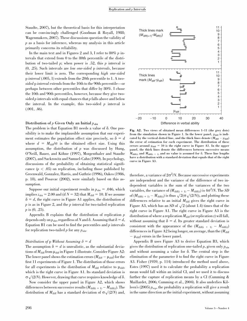
The assumption d 5 d is unrealistic, as the substantial devia-

tions of Mdiff from mdiff in Figure 1 illustrate. Consider Figure A2:

The lower panel shows the estimation errors (Mdiff� mdiff) for the

first 11 experiments of Figure 1. The distribution of those errors

for all experiments is the distribution of Mdiff relative to mdiff,

which is the right curve in Figure A1. Its standard deviation is

sp

(2/N). However, drawing that curve requires knowledge of d.

Now consider the upper panel in Figure A2, which shows

differences between successive results (Mdiff(i 1 1)�Mdiff(i)). The

distribution of Mdiff has a standard deviation of sp

(2/N) and,

therefore, a variance of 2s2/N. Because successive experiments

are independent and the variance of the difference of two in-

dependent variables is the sum of the variances of the two

variables, the variance of (Mdiff(i 1 1)�Mdiff(i)) is 4s2/N. The SD

of (Mdiff(i 1 1)�Mdiff(i)) is thusp

2(sp

(2/N)), and plotting these

differences relative to an initial Mdiff gives the right curve in

Figure A3, which has an SD ofp

2 (about 1.4) times that of the

right curve in Figure A1. The right curve in Figure A3 is the

distribution of where a replication Mdiff (or replication z) will fall,

without assuming that d 5 d. Its greater standard deviation is

consistent with the appearance of the (Mdiff(i 1 1) � Mdiff(i))

differences in Figure A2 being longer, on average, than the (Mdiff

� mdiff) errors in the lower panel.

Appendix B uses Figure A3 to derive Equation B3, which

gives the distribution of replication one-tailed p, given only pobt

and without assuming a value for d. The central step is the

elimination of the parameter d to find the right curve in Figure

A3. Fisher (1959, p. 114) introduced the method used above,

Estes (1997) used it to calculate the probability a replication

mean would fall within an initial CI, and we used it to discuss

further the capture of replication means by a CI (Cumming &

Maillardet, 2006; Cumming et al., 2004). It also underlies Kil-

leen’s (2005) prep, the probability a replication will give a result

in the same direction as the initial experiment, without assuming

123456789

1011

123456789

1011

−20 −10 0 10 20 30 40


Thick lines mark (Mdiff(i+1)-Mdiff(i))

Thick lines mark (Mdiff-µdiff)

µdiff

Fig. A2. Two views of obtained mean differences 1–11 (the grey dots)from the simulation shown in Figure 1. In the lower panel, mdiff is indi-cated by the vertical dotted line, and the thick lines denote (Mdiff � mdiff)the error of estimation for each experiment. The distribution of theseerrors around mdiff 5 10 is the right curve in Figure A1. In the upperpanel, the thick lines denote the differences between successive meansMdiff(i) and Mdiff(i 1 1) and no value is assumed for d. These line lengthshave a distribution with a standard deviation that equals that of the rightcurve in Figure A3.



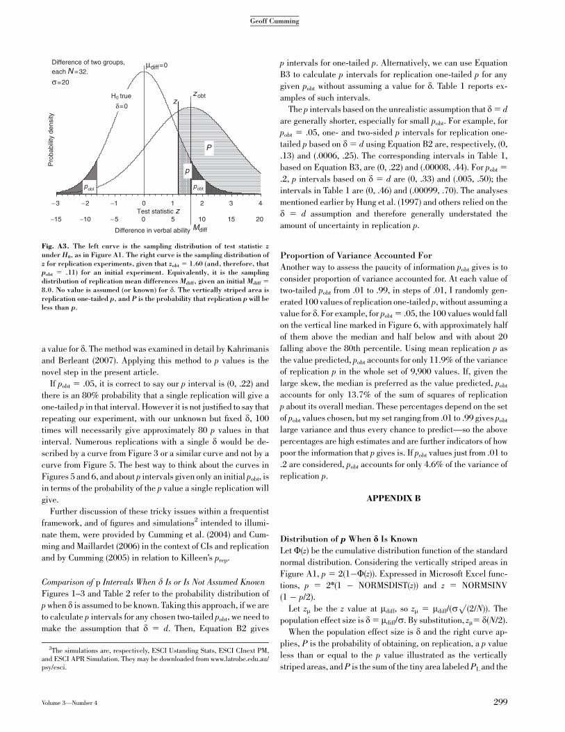
a value for d. The method was examined in detail by Kahrimanis

and Berleant (2007). Applying this method to p values is the

novel step in the present article.

If pobt 5 .05, it is correct to say our p interval is (0, .22) and

there is an 80% probability that a single replication will give a

one-tailed p in that interval. However it is not justified to say that

repeating our experiment, with our unknown but fixed d, 100

times will necessarily give approximately 80 p values in that

interval. Numerous replications with a single d would be de-

scribed by a curve from Figure 3 or a similar curve and not by a

curve from Figure 5. The best way to think about the curves in

Figures 5 and 6, and about p intervals given only an initial pobt, is

in terms of the probability of the p value a single replication will

give.

Further discussion of these tricky issues within a frequentist

framework, and of figures and simulations2 intended to illumi-

nate them, were provided by Cumming et al. (2004) and Cum-

ming and Maillardet (2006) in the context of CIs and replication

and by Cumming (2005) in relation to Killeen’s prep.

Comparison of p Intervals When d Is or Is Not Assumed Known

Figures 1–3 and Table 2 refer to the probability distribution of

p when d is assumed to be known. Taking this approach, if we are

to calculate p intervals for any chosen two-tailed pobt, we need to

make the assumption that d 5 d. Then, Equation B2 gives

p intervals for one-tailed p. Alternatively, we can use Equation

B3 to calculate p intervals for replication one-tailed p for any

given pobt without assuming a value for d. Table 1 reports ex-

amples of such intervals.

The p intervals based on the unrealistic assumption that d5 d

are generally shorter, especially for small pobt. For example, for

pobt 5 .05, one- and two-sided p intervals for replication one-

tailed p based on d 5 d using Equation B2 are, respectively, (0,

.13) and (.0006, .25). The corresponding intervals in Table 1,

based on Equation B3, are (0, .22) and (.00008, .44). For pobt 5

.2, p intervals based on d 5 d are (0, .33) and (.005, .50); the

intervals in Table 1 are (0, .46) and (.00099, .70). The analyses

mentioned earlier by Hung et al. (1997) and others relied on the

d 5 d assumption and therefore generally understated the

amount of uncertainty in replication p.

Proportion of Variance Accounted For

Another way to assess the paucity of information pobt gives is to

consider proportion of variance accounted for. At each value of

two-tailed pobt from .01 to .99, in steps of .01, I randomly gen-

erated 100 values of replication one-tailed p, without assuming a

value for d. For example, for pobt 5 .05, the 100 values would fall

on the vertical line marked in Figure 6, with approximately half

of them above the median and half below and with about 20

falling above the 80th percentile. Using mean replication p as

the value predicted, pobt accounts for only 11.9% of the variance

of replication p in the whole set of 9,900 values. If, given the

large skew, the median is preferred as the value predicted, pobt

accounts for only 13.7% of the sum of squares of replication

p about its overall median. These percentages depend on the set

of pobt values chosen, but my set ranging from .01 to .99 gives pobt

large variance and thus every chance to predict—so the above

percentages are high estimates and are further indicators of how

poor the information that p gives is. If pobt values just from .01 to

.2 are considered, pobt accounts for only 4.6% of the variance of

replication p.

APPENDIX B

Distribution of p When d Is Known

Let F(z) be the cumulative distribution function of the standard

normal distribution. Considering the vertically striped areas in

Figure A1, p 5 2(1�F(z)). Expressed in Microsoft Excel func-

tions, p 5 2n(1 � NORMSDIST(z)) and z 5 NORMSINV

(1 � p/2).

Let zm be the z value at mdiff, so zm 5 mdiff/(sp

(2/N)). The

population effect size is d5 mdiff/s. By substitution, zm5 d(N/2).

When the population effect size is d and the right curve ap-

plies, P is the probability of obtaining, on replication, a p value

less than or equal to the p value illustrated as the vertically

striped areas, and P is the sum of the tiny area labeled PL and the

p

P

zobtH true

δ=0z

p p

Test statistic z

Pro

babi

lity

dens

ity


Difference of two groups, each N =32.

σ=20

20151050−5−10−15

−3 −2 −1 0 1 2 3 4

Mdiff

µdiff=0

Fig. A3. The left curve is the sampling distribution of test statistic zunder H0, as in Figure A1. The right curve is the sampling distribution ofz for replication experiments, given that zobt 5 1.60 (and, therefore, thatpobt 5 .11) for an initial experiment. Equivalently, it is the samplingdistribution of replication mean differences Mdiff, given an initial Mdiff 5

8.0. No value is assumed (or known) for d. The vertically striped area isreplication one-tailed p, and P is the probability that replication p will beless than p.

2The simulations are, respectively, ESCI Ustanding Stats, ESCI CInext PM,and ESCI APR Simulation. They may be downloaded from www.latrobe.edu.au/psy/esci.


Geoff Cumming

horizontally striped area PR at right. Therefore P 5 1� F(zm 1

z) 1 F(zm� z). Alternatively,

P ¼1� NORMSDISTðzm þ NORMSINVð1� p=2ÞÞþ NORMSDISTðzm � NORMSINVð1� p=2ÞÞ: ðB1Þ

Equation B1 can be used to plot the cumulative distribution

function of the two-tailed p value or the probability density

function, which is shown in Figure 2 for d5 0.5 (N 5 32). In this

case, zm 5 dp

(N/2) 5 2, as in Figure A1 and the example in

Figure 1. Enter those values and p 5 a 5 .05 in Equation B1 to

confirm the power is .52.

Equation B1 depends on zm 5 dp

(N/2), which is the sepa-

ration between the two curves in Figure A1. As d increases from

0, power increases monotonically. Therefore, assuming that d�0, a given power determines d

p(N/2), which in turn determines

via Equation B1 the distribution of p, which is thus independent

of N and dependent only on power. Figure 4 can therefore show

the percentages of p for particular values of power with no

mention of d or N.

For completeness, I note the relationship for d known for one-

tailed p is as follows:

P ¼ NORMSDISTðzm � NORMSINVð1� pÞÞ: ðB2Þ

Distribution of p Given Only an Initial pobt

First, assume d 5 d, or equivalently that zm 5 zobt. Note that zobt

5 dp

(N/2), where d is the effect size in the initial experiment.

Then Equations B1 and B2 give, respectively, the distributions

of two-tailed and one-tailed p. Note that zobt 5 NORMSINV(1�pobt/2), with zobt� 0, so the distributions of p are dependent only

on pobt and not on N.

Now drop the d 5 d assumption. Considering Figure A3, the

relation for replication one-tailed p is as follows:

P ¼ NORMSDISTððzobt � NORMSINV

ð1� pÞÞ=SQRTð2ÞÞ:ðB3Þ

For completeness, I note the relation for replication two-tailed

p is as follows:

P ¼ 1� NORMSDISTððzobtþNORMSINVð1� p=2ÞÞ=SQRTð2ÞÞ þ NORMSDISTððzobt

� NORMSINVð1� p=2ÞÞ=SQRTð2ÞÞ:

ðB4ÞSubstitute zobt 5 NORMSINV(1� pobt/2) in Equations B3 and

B4 to confirm that, when we do not assume d5 d, P depends only

on pobt and not on N. Also, use Equation B4 to calculate that,

when pobt 5 .03, the probability is .561 that the replication two-

tailed p is less than .05, as mentioned in the section p Values,

Statistical Reform, and Replication.

Dropping the Assumption That s Is Known

For a known s, two groups with 32 participants each is equiv-

alent to a single group of 16. Figures 1–3, A1–A3, and all p

intervals are the same for a single group experiment (with N 5

16) as they would be for a two group experiment with N 5 32 for

each group. To investigate the simplest case of s not being

known, I considered a single group experiment for various val-

ues of N.

If we drop the assumption that s is known, the sample stan-

dard deviation (s) is used to estimate s. The left curve in Figure

A1 becomes the central t distribution, with df 5 N� 1, where N

is the size of the single group, and the right curve becomes the

noncentral t distribution, with df 5 N � 1 and noncentrality

parameter D ¼ dffiffiffiffi

Np

. Cumming and Finch (2001) described

noncentral t and its uses. Equations analogous to B1 and B2

allow calculation of the distribution of p, for a known d or if it is

assumed that d 5 d. For N 5 10, p intervals are somewhat

narrower than they are for the known s analysis, especially for

small pobt. Overall, however, the results are similar, and broad

conclusions from my main discussion assuming s known very

largely apply also for an unknown s, at least for single groups

down to N 5 10.

Verification of Numerical Results

Equations B1 and B2 give results that agree with replication

one-tailed p and mean p values for a range of percentiles and

values of power reported by Hung et al. (1997, Tables 1, 2, and

3), post hoc power for one-tailed a 5 .025 (although mislabeled

as .05) for a range of pobt values reported by Posavac (2002, Table

2), two-tailed post hoc power reported by Goodman (1992, Table

1, column 2), and quartiles for p reported by Morgenthaler and

Staudte (2007, p. 9).

In addition, I tested my results by simulation. For each of a

selection of pobt values, I generated data from 100,000 experi-

ments and found percentiles for the empirical distribution of

100,000 p values. The results agreed with my calculated values,

for both one- and two-tailed p, for d known, and for d not known

without assuming d 5 d. I similarly confirmed by simulation my

calculations when s is not assumed known and N 5 10.



Replication and p · PDF fileReplication and p Intervals p Values Predict the Future Only...

Documents

Transcript of Replication and p · PDF fileReplication and p Intervals p Values Predict the Future Only...