Electronic copy available at: http://ssrn.com/abstract=2268215

Location, Location, Location:

Repetition and Proximity Increase Advertising E�ectiveness∗

Garrett A. Johnson, Randall A. Lewis, and David H. Reiley†

January 9, 2014

Abstract

Yahoo! Research partnered with a nationwide retailer to study the e�ects of online display

advertising on both online and in-store purchases. We measure the impact of frequency of

advertising exposure using a simple randomized experiment: users in the `Full' treatment group

see the retailer's ads, users in the `Control' group see unrelated control ads, and users in the

`Half' treatment group see an equal probability mixture of the retailer and control ads. We

�nd statistically signi�cant evidence that the retailer ads increase sales 3.6% in the Full group

relative to the Control. We �nd strong bene�ts to repeated exposures among the 80% of users

who see up to 50 ads per person, as revenues increase approximately linearly with a marginal

bene�t of around 5¢ per exposure. We �nd especially high ad e�ectiveness for the retailer's

best customers and those who live closest to its brick-and-mortar locations; these �ndings are

consistent with a model of advertising in a Hotelling model of di�erentiated �rms.

JEL: M37, M31, C93, L86

∗This paper was previously released under the title �Add More Ads? Experimentally Measuring IncrementalPurchases Due To Increased Frequency of Online Display Advertising.�†Johnson: Simon Business School, University of Rochester, <Garrett.Johnson@Simon.Rochester.edu>.

Lewis: <randall@econinformatics.com>, 1600 Amphitheatre Parkway, Mountain View, CA 94043. Reiley:<david@davidreiley.com>, 1600 Amphitheatre Parkway, Mountain View, CA 94043. The authors performed thisresearch while employed at Yahoo! Research. We acknowledge Yahoo! both for its �nancial support and for its sup-port of unbiased scienti�c research through its ex-ante decision to allow us to publish the results of the experimentno matter how they turned out. We would like to thank Valter Sciarillo, Jennifer Grosser Carroll, Taylor Schreiner,Eddie Babcock, Iwan Sakran, and many others at Yahoo! and at our client retailer who made this research possible.We thank Eric Anderson, Susan Athey, Ben Jones, Preston McAfee, Rob Porter, Justin Rao, and Elie Tamer forhelpful discussions and Mary Kraus for proofreading.

1

Electronic copy available at: http://ssrn.com/abstract=2268215

1 Introduction

How much advertising should �rms purchase, and to whom should they target their advertising?

Advertisers assume that diminishing returns set in once a consumer has seen enough ads, but adver-

tisers disagree over what constitutes `enough.' Advertisers also disagree over whether advertising

should target a �rm's best customers, or whether it should instead attempt to convert marginal

customers into more lucrative customers. In this paper, we shed light on these issues by running a

large-scale controlled experiment on Yahoo!. We examine two consecutive weeklong ad campaigns

that target three million of the retailer's existing customers. Our experiment breaks new ground

in its large scale and in its combination of consumer-level ad exposure with retail purchase data.

Our experimental estimates suggest the retailer ads increased sales by 3.6% and that the campaigns

were pro�table. On the question of ad frequency, we experimentally vary the intensity of treatment

and �nd that `enough' is higher than many expect: the returns to advertising appear constant even

out to 50 ad exposures in two weeks. We also show that the retailer ads generate the largest sales

lift among the retailer's best customers and those who live near a store. Thus, as our intention-

ally punny title suggests, both repetition and proximity (in geographic or abstract product space)

produce bene�ts in advertising.

Controlled experiments are the only unbiased way to measure ad e�ectiveness. Though a report

commissioned by the Interactive Advertising Bureau upholds this view (Lavrakas, 2010), controlled

experiments remain rare in the industry. This dearth of experiments seems surprising given the

dollars at stake: advertising represents between 1% and 2% of global GDP (Bughin and Spittaels,

2012), and online display advertising alone represents $7.7 billion (IAB, 2013). Nonetheless, exper-

iments are costly to plan, operate, and analyze. These costs increase further when one wishes to

directly measure returns using purchase outcomes rather than proxy measures like survey-based pur-

chase intent. Furthermore, Lewis and Rao (2013) argue that the e�ect of advertising on purchases is

statistically di�cult to detect even when the true e�ect is economically large. They observe that the

mean impact of advertising is plausibly a small fraction of the variance in sales in settings like ours.

Such experimental ad e�ectiveness studies therefore have low statistical power and may require

millions of observations�across consumers, campaigns, or time�to detect a pro�table campaign.

Despite these challenges, ad experiments remain valuable relative to observational studies, which

2

are prone to biases that undercut their usefulness. Observational studies estimate ad e�ects by

comparing exposed users to unexposed users. Advertiser choices can induce bias, for instance, by

targeting customers who are more likely to purchase or by targeting times like Christmas when

customers purchase more. In our anteceding ad experiment, Lewis and Reiley (2013) show that the

observational estimate had the wrong sign. Lewis, Rao and Reiley (2011) show that consumer choices

online can also induce what they term `activity bias' which occurs because consumer browsing is

correlated across websites.

We designed our experiment primarily to examine the shape of the consumer ad frequency

response curve. The experiment includes a `Full' treatment group that is exposed to the retailer's

ads and a `Control' group that is exposed to unrelated, control ads. We also include a `Half'

treatment group that sees a mixture of the retailer and control ads with equal probability. The

control ads allow us to separate the impact of ad frequency from `ad type,' by which we mean the

user's eligibility to see ads based on her browsing intensity. We also collect data on consumer location

and past sales to examine heterogeneous ad e�ects. In all, our experiment includes over three million

joint customers of Yahoo! and the retailer, of which 55% are exposed to an experimental ad.

Our controlled ad experiment is among the largest and most statistically powerful in the ad

e�ectiveness literature. Split-cable television studies examine ad e�ectiveness using a panel of

3,000 viewers combined with data on consumer-packaged-good purchases (see Lodish et al. (1995)).

These studies have low statistical power: meta-analyses of over 600 such tests reveal that the

majority failed to demonstrate statistically signi�cant ad e�ects at conventional levels (Lodish et

al., 1995; Hu et al., 2007). Sahni (2012) examines the impact of display ads on sales leads within an

Indian restaurant search website. The study examines eleven separate experiments involving several

thousand users, which are su�ciently powerful because they target consumers who are in-market for

a restaurant. Other Internet advertising experiments such as Blake et al. (2013) (search advertising)

involve thousands or possibly millions of users but vary treatment over time or across markets rather

than across consumers. Though sales data are rare in the literature, our experiment�similar to

the previous Lewis and Reiley (2013) experiment with the same retailer�links ad exposure data

to both online and in-store sales data at the individual level. We improve on the Lewis and Reiley

(2013) by doubling the sample size to three million customers and by improving the experimental

design with control ads.

3

Our overall results suggest that the retailer ads increased sales and that the campaign was

pro�table. Our experimental estimates suggest an average sales lift of $0.477 on the Full treatment

group and $0.221 on the Half treatment group, which represent a 3.6% and a 1.7% increase over the

Control group's sales. Each ad impression cost about 0.5¢, and the average ad per-person exposure

was 34 and 17 in the Full and Half groups. Assuming a 50% retail markup, the ad campaign yielded

a 51% pro�t, though pro�tability is not statistically signi�cant (p-value: 0.25, one-sided).

A varied literature considers whether the ad frequency curve exhibits increasing, constant, or

decreasing returns to scale. Much ad frequency research relies on observational or lab studies (see

Pechmann and Stewart, 1988, for a survey). Several recent papers use experiments to examine ad

frequency. Lewis (2010) examines the frequency curves of online display ads for clicks and conver-

sions using natural experiments reaching tens of millions of Yahoo! users. He �nds heterogeneous

frequency e�ects among campaigns: a third demonstrate constant returns for over 20 ad exposures,

and the rest exhibit some degree of wear-out. Sahni (2013) experimentally varies treatment intensity

and �nds decreasing returns to online display ads after only three exposures in a session.

We �nd constant returns to ad frequency for users who are eligible to see 50 ads or less. These

users represent over 80% of the treated population. We measure the marginal value of an additional

ad to be 3.68¢ for this subpopulation. The experiment allows us to test several otherwise untestable

assumptions about the impact of frequency. These assumptions include linear returns to ad fre-

quency and no impact from ad type for users eligible to see up to 50 ads. These assumptions do

not meaningfully change our marginal ad frequency estimate (3.71¢) but boost its precision. With

greater precision, we show that the overall campaign was pro�table at the 5% signi�cance level: the

incremental pro�t accrued over four weeks from those consumers who were eligible to see up to 50

ads more than o�sets the cost of the entire campaign. Our results contrast with the wear-out result

of Sahni (2013), though our advertising time period is longer and our outcome is subsequent sales

rather than instantaneous sales-leads. However, Lewis (2010) also found that some campaigns for

well-known nationwide brands exhibit constant returns to over 50 exposures on a single day.

Finally, we consider a model of advertising by Grossman and Shapiro (1984) within a Hotelling

model of di�erentiated �rms. Their model concludes that a �rm's advertising most a�ects consumers

who are `near' the �rm or are already inclined toward a �rm's product. We test this implication

using both consumer's geographic proximity to the retailer's stores and proximity in terms of the

4

consumer's taste for the retailer. For the latter, we examine multiple revealed preference measures

including the consumer's monetary value, purchase recency, and income. We con�rm the Grossman

and Shapiro (1984) prediction that proximity mediates ad e�ectiveness in all four proximity mea-

sures. Our geographic proximity results accord with those of Molitor et al. (2013) who �nd that

mobile coupon redemption rates increase as consumers get closer to the store. Our monetary value

result contrasts with experimental studies in catalog advertising (Anderson and Simester, 2004) and

search advertising (Blake et al., 2013) that �nd advertising is less e�ective on the advertiser's high-

value customers. We speculate that our results di�er because our data includes sales through both

online and o�ine channels and because our retailer advertises less often, which reduces cumulative

wear-out.

We improve our experimental methodology in order to gain statistical precision in our results.

We use the control ads not only to identify the counterfactual subpopulation who sees the ads, but

also the �rst day that each user is exposed. With this, we can �lter out both unexposed users and

pre-exposure sales in our experimental di�erence. These improvements boost our precision by 31%

without inducing bias. This boost exceeds the 5% improvement yielded by including a myriad of

covariates in our linear regression in order to reduce the residual variance.

The rest of this paper is organized as follows. The next section describes our experimental design

and data collection. The third section gives an overview of the data and some descriptive statistics.

The fourth section presents our measurements of the causal e�ects of the advertising, particularly

about the e�ects of frequency, as well as heterogeneous treatment e�ects by consumer proximity.

The �nal section concludes.

2 Experimental Design

The experiment measures ad e�ectiveness for a national apparel retailer advertising on Yahoo!. The

experiment took place during two consecutive weeks in spring 2010. In each week, the advertisements

featured a di�erent line of branded clothing. The experimental subjects were randomly assigned to

treatment groups that remained constant for both weeks. A con�dentiality agreement prevents us

from naming either the retailer or the featured product lines.

To investigate the e�ects of exposure frequency, our experiment uses three treatment groups that

5

vary the treatment intensity. The `Full' treatment group is exposed to the retailer's ads while the

`Control' group is exposed to unrelated control ads. A third, `Half' treatment group is, on average,

exposed to half of the retailer and control ads of the other two groups. We implemented this design

by booking 20 million retailer ads for the Full group, 20 million control ads for the Control group,

and both 10 million retailer ads and 10 million control ads for the Half group.1 Each experimental

ad exposure in the Half group therefore has a 50% chance of being a retailer ad and a 50% chance

of being a control ad. This experimental design enables us to investigate the impact of doubling the

number of impressions in a campaign. Doubling the size of the campaign increases ad delivery on

two margins: 1) showing more ads to the same consumers (the intensive margin) and 2) increasing

the number of consumers reached, here by 8% (the extensive margin). The average ad frequency in

the Half group is comparable to a typical campaign for this retailer on Yahoo!.

The experiment employs control ads to identify the counterfactual ad exposures that a consumer

could have seen if they were assigned to the Full retailer campaign. The control ads also identify

the counterfactual treated subgroup so that we can measure more precisely the Average Treatment

E�ect on the Treated (ATET). Without control ads, Lewis and Reiley (2013) compute the ATET

indirectly by di�erencing the average outcomes of consumers assigned to treatment from the average

of those assigned to the control group (intention to treat) and then dividing by the probability of

receiving treatment. Though the two estimators of ATET are both consistent, the indirect measure

is less e�cient from including noise from the di�erence in outcomes among the untreated subgroups.

The experiment's subjects are existing customers of both Yahoo! and the retailer. Prior to the

experiment, a third-party data-collection �rm matched a list of customers using name and address

(either terrestrial or email). Leveraging additional customer records, the third-party doubled the

number of matched customers from the 1.6 million customers studied by Lewis and Reiley (2013) to

3.3 million in the present experiment. After the experiment ended, the third-party �rm combined

the retailer's sales data and the Yahoo! advertising data and removed identifying information to

protect customer privacy.

Due to an unanticipated problem in randomly assigning treatment to multiple matched con-

1These campaigns were purchased on an impression, not click, basis. This avoids distortions induced by ad serverschanging delivery patterns in the treatment and control groups due to the retailer and control ads having di�erentclick-through rates. Purchasing ads based on a cost-per-click or cost-per-action basis can introduce such distortionswhen using control ads to tag counterfactual exposures in the control group.

6

sumers, we exclude almost 170,000 customers from our analysis. In particular, the third-party data

collection �rm joined 3,443,624 unique retailer identi�ers with 3,263,875 unique Yahoo! identi�ers;

as a result, tens of thousands of Yahoo! identi�ers were matched with multiple retail identi�ers.

The third party performed the experimental randomization on the retailer identi�ers, but provided

Yahoo! only with separate lists of Yahoo! identi�ers for each treatment group to book the cam-

paigns. Some multiple matched Yahoo! users were therefore accidentally booked into multiple

treatment groups, which contaminated the experiment. To avoid this contamination, we discard

all the Yahoo! identi�ers who are matched with multiple retailer identi�ers.2 Fortunately, the

treatment-group assignment is random, so the omitted consumers do not bias the experimental

estimates. The remaining 3,096,577 uniquely matched Yahoo! users represent our experimental

subjects. We acknowledge that our results only re�ect 93% of exposed users.

The retailer ads are primarily image advertising and are co-branded with apparel �rms. The ads

display the store brand, the brand of the featured product line, and photographs of the advertised

clothing line on attractive models. The creative content of each ad impression is dynamic and

involves slideshow-style transitions between still photographs and text. Campaign 1 includes three

di�erent ads in an equal-probability rotation: men's apparel, women's apparel, and women's shoes.

Campaign 2 advertises a product line from a di�erent manufacturer and features women's apparel.

Consequently, we acknowledge that our ad frequency results refer to repeated ad exposures from

the same retailer but re�ect signi�cant creative rotation. The control ads advertise Yahoo! Search.3

The experiment's ads appear on all Yahoo! properties, such as Mail, News, Autos, and Shine.

The ads take four rectangular formats. We ensure the distributions of ad formats and placements

are the same for all three treatment groups.

2We also perform the analysis on all uncontaminated customers assigned to a single group (results availablefrom the authors upon request). We weight these customers to ensure the results represent the intended campaignaudience. The re-weighting scheme increases the weight on multiple match consumers assigned to a single treatment.For example, a customer with three retailer identi�ers who is assigned exclusively to the Full group receives a weightof nine in the regression, because uncontaminated customers represent three out of 27 possible combinations of tripletreatment assignments. The results are qualitatively similar to those presented here, but statistically less precise. Theweighted estimator has higher variance because the overweighted customers have higher variance in their purchases.For expositional clarity and statistical precision, we opt to discard multiple matched consumers here. Note that ourpoint estimates of ad e�ectiveness are generally higher in the weighted analysis, so our preferred set of estimates aremore conservative.

3The Yahoo! Search ad demonstrates an animated search for the rock band `The Black-Eyed Peas' and emphasizesboth the search links and multimedia content that Yahoo! Search provides. The animation ends with an in-ad,functioning search box. The control ads are the same for both weeks.

7

3 Data

The data section contains three subsections. The �rst describes our data and demonstrates that

our experimental randomization is valid. The second presents a power calculation that shows the

di�culty of measuring ad e�ectiveness in our setting. The third section details the source of our

data and explains how we generate some of our key variables.

3.1 Descriptive Statistics

Table 1 provides summary statistics for the experiment. Over three million customers were evenly

assigned to one of our three treatment groups: Full, Half, or Control. Ad exposure depends on

a user's browsing activity during the two weeks of the campaign. 55% of users were exposed to

an experimental ad. The summary statistics in Table 1 are consistent with a valid experimental

randomization. In each treatment group 68.5% of customers are female, the average age is 43.6 years,

and customers viewed an average of 122 web pages on Yahoo! during the campaign. Customers

spent an average of $19.23 at the retailer during the two weeks prior to the experiment and $857.53

in the two years beforehand.4 Figure 1 shows that the consumer proximity to the nearest retailer is

distributed near identically across treatment groups.5 On average, treated consumers live 21 miles

from the nearest retailer location, but half (median) live within 6.6 miles.

In Table 1, we see that the experiment delivers advertisements evenly across treatment groups.

48.3% of users are exposed to Campaign 1, 48.8% are exposed to Campaign 2, and 55.4% see ads in

at least one campaign. Campaign 1 delivers 13% more ad impressions per person than Campaign

2, but reaches 1% fewer customers. For the remainder of this section, our descriptive statistics

exclude the unexposed users. Figure 2 shows that the distribution of total ad views (both retailer

and control) across the three treatments is identical. The distribution of ad views is highly skewed

towards the left, so that the mean is 33 while the median is 15. As expected, the Half treatment

group sees an even split of retailer and control ads. On average, the exposed subjects saw an

experimental ad on 16.3% of the pages they visited on Yahoo!.6 The maximum number of ad views

was 23,281, which we suspect was caused by automated software (i.e., a `bot') running on that user's

4An F -test for the null hypothesis of equality of the means between the three treatment groups gives p-values forthese �ve variables of 0.794, 0.607, 0.132, 0.485, and 0.517 respectively.

5A Kolmogorov-Smirnov test of Control CDF versus combined CDF of Half and Full gives p = 0.74.6Users who see at least one ad visit an average of 205.6 pages on Yahoo! during the two week experiment.

8

computer since the �gure implies about 10,000 daily webpage visits. Though ads do not in�uence

bots, we keep these observations in our analysis both because the appropriate cuto� is not obvious

and because the upper tail of the distribution is small.7

Table 1 also describes clicks on the retailer's ads. The click-through rate, the quotient of clicks

and ad views, is 0.17% for Campaign 1 and 0.22% for Campaign 2 in the Full group. These click-

through rates are high: many online display advertising campaigns have click-through rates under

0.1% (Lewis, 2010). The clicker rate, the fraction of exposed users who click on any ad, is 2.9% for

Campaign 1 and 3.2% for Campaign 2 in the Full group. The Half treatment group's clicker rates

are lower because its subjects have fewer opportunities to click an ad.

Histograms show that the distribution of pre-treatment sales are essentially identical across all

three treatment groups. Figure 3 illustrates the distribution of average weekly sales over the two

years prior to the experiment. Figure 4 shows the distribution of individual purchases conditional on

transactions in the two weeks prior to the experiment. To better visualize the distribution, Figure 4

omits the 90.8% of observations with zero purchases in the two weeks; 0.96% of purchase amounts

are negative, which represents returns to the store net of any purchases.

Figure 5 shows sales for the three treatment groups during the two-week experiment, excluding

customers with zero purchases. Figure 5 shows how the e�ect of advertising is small relative to

overall sales, even though the estimated lift is economically substantial relative to the ad cost.

We can distinguish a slight shift in the distribution to higher levels of purchases: negative net

purchase amounts are less frequent in the treatment groups than the control group, while purchase

amounts larger than $200 appear more frequent in the treatment groups. We see that we are at the

measurement frontier for detecting the treatment e�ect of ads on sales.

3.2 Power Calculation

Since our sample is much larger than most experimental studies, we wish to temper the reader's

expectations regarding the strength of our experimental results. The experiment's statistical power

is limited, even though our experiment includes three balanced treatment groups with about 570,000

treated users each. For a comprehensive discussion of the statistical power issue, we refer the

7Less than 2% of users saw more than 1,000 page views. A few extreme outliers cause average page views and adviews to di�er across treatment groups in the third decimal place, contributing to the relatively low p-value mentionedfor page views in footnote 4.

9

reader to the meta-analysis by Lewis and Rao (2013) of 25 experiments measuring online display

ad e�ectiveness.

To demonstrate the limits of our experiment, we present a statistical power calculation for

testing the null hypothesis that advertising has no impact on sales. In the calculation, we consider

the alternative hypothesis that the advertiser receives a 50% return on its advertising investment.

The alternative hypothesis implies an average treatment e�ect on the treated of $0.51 in the Full

treatment group given the $0.17 cost of display ads and assuming a 50% gross margin for the retailer.

That is, the null and alternative hypotheses are

H0 : ∆sales = $0

Ha : ∆sales = $0.51,

To determine power, we �rst calculate the expected t-statistic under this alternative. The standard

deviation of sales is $125 for the two-week campaign and the sample size is 570,000 in each of the

Full and Control treatment groups. The expected t-statistic is given by

E[T ] =δ̂ − δ0SE

(δ̂) =

0.51− 0125√2√

570,000

= 2.18

for the average treatment e�ect estimator δ̂.8 Using the 10% two-sided critical value of t? = 1.645,

the power of the test is given by

Pr(T > t?|E[T ] = 2.18) = 70%

An analogous test for the Half group only has power of 29%.9 We emphasize that the above calcu-

lations are about whether the ads impact sales: a test of pro�tability has much less power because

8Let µ̂ denote the sample average and σ2 the variance of N consumer sales observations. Let the subscripts T andC denote the Treatment and Control groups. The standard error of the treatment e�ect estimator δ̂ is given by thesquare root of its variance

V ar(δ̂)

= V ar (µ̂T − µ̂C) =σ2T

NT+σ2C

NC=

2σ2

N

where we assume that NT = NC and σ2T = σ2

C , which is a good approximation here.9The alternative hypothesis for the Half group e�ect is ∆sales = $0.255 with E [T ] = 0.255−0

125√

2√570,000

= 1.09. The

associated power is Pr(T > t?|E[T ] = 1.09) = 29%.

10

it requires gross pro�ts to exceed positive costs, rather than zero. The above power calculations

elucidate both the limits of our experimental results and the importance of improving the precision

of our treatment e�ect estimates. In Section 4.2, we describe several econometric methods designed

to improve precision.

3.3 Data Source

Our experiment resolves many traditional problems in measuring ad e�ectiveness. First, advertisers

typically cannot identify the consumers who see their ads. We address this by restricting our

experiment to logged-in, identi�able Yahoo! users. Second, advertisers rarely possess consumer-

level data that links ad exposure to purchases. Our data are rare in that they combine sales data

from the retailer�both online and in-store�with ad delivery and demographic data from Yahoo!

at the consumer level.

We measure the e�ect of advertising on the retailer's relevant economic outcome�actual purchases�

by relying on the retailer's customer-level data. The retailer believes that its data correctly attributes

more than 90% of all purchases to individual customers by using all the information that they pro-

vide at check-out (credit-card numbers, phone numbers, etc.). We collect purchase data before,

during, and after the campaigns.

We improve on the statistical precision of our predecessor (Lewis and Reiley, 2013) by collecting

both more granular sales data and sales data over a longer period of time. First, we obtain daily

rather than weekly transactions during the ad campaigns. Daily transaction data allow us to discard

purchases that take place prior to a customer's �rst ad exposure. Since pre-exposure transactions

could not be in�uenced by the advertising, including such transactions in our treatment e�ect

estimates only adds noise. This strategy avoids sample-selection problems, because the control ads

identify the corresponding pre-treatment sales in the control group.10 Second, we obtain consumer

purchase data for the two years prior to the experiment.11 We use the purchase history as covariates

10If the ads a�ect behavior, this could create a selection e�ect that distorts the composition of the exposed sampleor the number of ads delivered. Suppose that consumers are more likely to click on the retailer ad than the controlad. The ad-server may then have fewer opportunities to deliver ads because the people who click on the retailer adare shopping rather than browsing Yahoo!. The summary statistics in Table 1 suggest, however, that ad exposureand browsing is su�ciently similar across groups that we can dismiss these concerns here.

11The data include weekly sales for the eight weeks before treatment. To save space, the retailer aggregated weeks9�44 before treatment into a single variable. We have weekly data for weeks 45�60 before treatment, to capture anysimilar variation across years during the weeks of the experiment. The data again aggregate weeks 61�104 beforetreatment into a single variable. Our data distinguishes between online and in-store sales throughout.

11

in our ATET regressions to reduce the variance of our experimental estimates.

We also examine how the e�ect of advertising varies with a customer's proximity to the nearest

retailer store. To compute proximity, we use nine-digit zip code data from Yahoo! and a third-party

data broker, which are available for 75.2% of the experimental subjects and 77.8% of the exposed

subjects. Each nine-digit zip code denotes a fraction of a city block, providing the �ne-grained

resolution required to investigate the e�ect of advertising within a mile of a store. We employ

a database from Yahoo! Maps to link nine-digit zip codes to latitude and longitude coordinates.

For each customer, we compute the `crow-�ies' distance to the nearest store using the haversine

formula.12

We also use demographic data. Yahoo! requests user gender, age, and state at sign-up. The

third-party data partner provided household income in �ve coarse strata.

4 Results

The results section is divided into four subsections. The �rst presents a high-level overview. The

second shows experimental estimates for the sales lift during the two weeks of the ad campaign. We

present methods that improve the statistical precision of our estimates in this low powered setting.

The second subsection analyzes the role of ad frequency on ad e�ectiveness. We apply gradually

more restrictive assumptions to measure ad frequency e�ects and show that these assumptions are

supported by the data. The third section examines heterogeneous treatment e�ects by consumer

proximity to the retailer. The �nal subsection collects additional results that break apart the e�ect

of advertising by the retailer's online and in-store channels, by individual ad campaign, and by

probability of purchase versus basket size.

4.1 Overview

We �nd evidence that the experiment's advertising causes a signi�cant increase in consumer sales.

Our preferred estimates suggest that consumers who were exposed to the retailer's ad saw their

average sales increase by $0.477 with standard error (s.e.) $0.204 in the Full treatment group and

$0.221 with s.e. $0.209 in the Half treatment group. These represent a 3.6% and 1.7% increase in

12The haversine formula calculates the distance between two pairs of latitude and longitude coordinates whilecorrecting for the spherical curvature of the planet.

12

sales above the Control group. The e�ect in the Full group is highly signi�cant (p-value, two-sided:

0.020), the Half group is not signi�cant (p-value: 0.289), and the joint test is marginally signi�cant

(p-value: 0.065). Though the e�ect in the Half group is 46.3% that of the Full group, an F-test for

equality of the two e�ects is not rejected at 10% (p-value: 0.211).

Our experimental evidence suggests that the ads were likely pro�table for the retailer. Given

about 570,000 exposed users in each of the three treatment groups, our preferred experimental

estimates and 95% con�dence interval implies a total sales lift of $273, 000 ± 229, 000 in the Full

group and $126, 000± 234, 000 in the Half group. The campaign cost the retailer about $88,000 for

the Full campaign and $44,000 for the Half campaign. To calculate pro�tability, we assume a gross

margin of 50% for the upscale retailer,13 but we ignore �xed advertising costs including creative

development. Our point estimates indicate a rate of return of around 50% on the advertising dollars

spent but the 95% con�dence interval extends from losing the entire investment to doubling it.

We also leverage the experimental variation in the consumer's retailer ad views (frequency) and

eligibility for ads (ad type) to measure the average impact of an additional retailer ad. We restrict

our analysis here to the 81% of consumers who see up to 50 total ads (retailer and control) for

whom our estimates are more precise. Our least restrictive assumptions suggest that an additional

ad has a 3.68¢ impact (s.e. 1.72¢). We also use the experiment to evaluate several assumptions that

relate ad e�ectiveness to frequency and ad type. Under these assumptions, our estimates suggest

the value of an additional ad is almost unchanged at 3.71¢ but more precisely estimated with a

standard error of 1.02¢.

We consider heterogeneous treatments by consumer proximity to the retailer in order to under-

stand the e�ect of advertising in a di�erentiated market. We test the predictions from the Grossman

and Shapiro (1984) model that consumers near the advertiser will be more a�ected by its advertis-

ing. We examine the ad e�ect by the consumer's geographic proximity to the retailer and `taste'

proximity to the retailer as captured by purchase recency, customer monetary value, and belonging

to the retailer's target income segment. We �nd large and statistically signi�cant ad e�ects within

the subpopulation who live within one mile of a retailer, transacted within eight weeks, spend more

than $1,000 at the retailer in the previous two years, or earn more than $100,000.

13We base this on conversations with retail experts, supplemented with references to similar retailers' �nancialstatements.

13

We further decompose the result by campaign, sales channel, and shopping trips. Our estimates

suggest the second weeklong campaign is more e�ective and demonstrates a statistically signi�cant

ad e�ect on its own (p-value: 0.012). We �nd that the majority of the total treatment e�ect is

attributable to the in-store rather than online sales channel: 68% in the Full group and 84% in the

Half group. We present descriptive evidence that decomposes the treatment e�ect into increased

probability of purchase versus basket size. Though these results are inconclusive, we are able to

detect a statistically signi�cant 1.8% increase in shopping trips in the Full group.

4.2 Overall Campaign Impact

Table 2 presents regression estimates of the Average Treatment E�ect on the Treated (ATET) for

the impact of advertising on consumer purchases during the two-week experiment. In particular,

Table 2 highlights the various methods for increasing the precision of the estimates. These methods

include pruning components of the outcome data that cannot be in�uenced by advertising and

introducing covariates into the regression. In all, we improve the precision of our estimates�or

shrink the standard errors�by 34% on average.

Table 2 begins with the indirect ATET estimate. The indirect ATET estimator takes the

treatment-control di�erences for the entire sample of 3.1 million consumers (intent-to-treat estimate)

and divides by the treatment probability (the 55.4% exposed subsample).14 The indirect ATET

estimator relies on the fact that outcomes among untreated subjects have an expected experimental

di�erence of zero. However, the di�erence among untreated subjects adds noise to the estimator.

The indirect ATET estimator yields a $0.67 average sales lift (s.e. $0.32) in the Full treatment

group and an average lift of $0.03 (s.e. $0.31) in the Half group. Whereas Lewis and Reiley (2013)

estimate the ATET indirectly out of necessity, this experiment employs control ads to identify the

counterfactual treated sample in the Control group.

Table 2's column 2 presents the direct ATET regression estimate on the treated subsample. The

direct ATET estimator increases precision by pruning the untreated subsample which contributes

only noise to the estimator. The regression shows that the Control group has $15.53 purchases

on average while the average purchases in the Full treatment group are $0.52 larger and those

14This is numerically equivalent to computing a local average treatment e�ect by using the random assignment asan instrument for treatment.

14

in the Half group are $0.19 larger. The Full treatment e�ect is statistically signi�cant (p=0.027,

two-sided), while the Half treatment is not (p=0.423). An F -test of joint signi�cance is marginally

signi�cant (p=0.082). The direct ATET requires control ads to identify the treated subgroup in the

Control, which improves the precision of the estimates by 25% on average.

Table 2's column 3 uses both the control ads and daily level sales data to further prune the data

and boost precision by another 8%. Speci�cally, we omit purchases that occur prior to a consumer's

�rst experimental ad exposure. This method is free from bias because ads cannot in�uence sales

until the user receives the ad and the control ads identify the counterfactual pre-treatment sales in

the Control group. Excluding irrelevant sales reduces the baseline average purchase amount from

$15.53 to $13.17 per person. The point estimates here are $0.56 (s.e.: $0.22) in the Full group and

$0.31 (s.e.: $0.22) in the Half group.

In columns 4�7 of Table 2, we increase the precision of our estimates by adding covariates to the

ATET regression. The covariates in the regression improve precision by reducing the unexplained

variance in the dependent variable.15 First, we add demographic covariates that include indicator

variables for gender, year of age, and state of residence as well as a scalar variable for the time

since the consumer signed up with Yahoo!. These covariates explain little of the variance in sales

illustrated by an R2 of 0.001, so the precision of the estimates is unchanged. Column 5 adds

retailer-de�ned customer segments: �ve categories for recency of last purchase, four categories for

frequency of past purchases, and four categories for total lifetime spending at the retailer. The

customer segments improve the R2 to 0.042, and increase precision by 2%. Column 6 adds two

years of individual-level past sales data and pre-treatment sales during the campaign, separately

for online and o�ine sales.16 Past purchases best explain the sales during the experiment as they

increase the R2 to 0.090, and the standard error for the Full treatment estimate falls a further 3%

on average. Table 2's Column 7 presents our preferred estimates, which include browsing intensity

covariates. Speci�cally, we include �xed e�ects for the total experimental ads delivered (ad type)

and indicators for the day of the consumer's �rst ad exposure.17 To the extent that shopping

behavior is correlated with current online browsing activity, the ad type �xed e�ects will improve

15Speci�cally, a regression model with a given R2 reduces the standard errors of our treatment e�ect estimates by1−√

1−R2.16Sales data provided at the level of individual weeks or aggregates of multiple weeks. See footnote 11.17The ad type covariates include indicator variables for ad types (total ad views) from 1 to 29 and a single indicator

variable for ad types of 30 or more.

15

e�ciency. These covariates marginally improve the R2 to 0.091 and decrease the point estimates

without noticeably increasing precision.

Including covariates improves precision by 5% (columns 3�7) across Full and Half groups, while

pruning irrelevant data improves precision by 31% (columns 1�3) on average.18 However, covariates

may be inexpensive to include and serve to validate the experimental randomization. Control ads are

expensive but facilitate data pruning and thereby improve precision �ve times over our covariates.

Our preferred estimator�in column 7 of Table 2�measures a $0.477 (s.e.: $0.204) increase in

average sales from the ads in the Full group and a $0.221 (s.e. $0.209) increase in the Half group.

The Full treatment e�ect is statistically signi�cant at the 5% level (p-value: 0.020) and represents a

nearly 3.6% sales lift over the Control group. The Half treatment e�ect is not signi�cantly di�erent

from zero (p-value: 0.289), and the joint F -test is marginally signi�cant (p-value: 0.065). The point

estimates indicate that doubling the advertising approximately doubles the e�ect on purchases,

but the precision of these estimates is too low to have much con�dence in the result. In the next

subsection, we use consumer-level variance in treatment intensity to better model the e�ect of ad

frequency. At this point, we cannot establish the campaign's pro�tability with con�dence.

Given 570,000 exposed users in each of the three treatment groups, our point estimates indicate

that the Full campaign increased retail purchases by a dollar value of $273, 000 ± 229, 000, while

the Half campaign increased purchases by $126, 000 ± 234, 000, using 95% con�dence intervals.

Compared with costs of about $88,000 for the Full campaign and $44,000 for the Half campaign,

these indicate incremental revenues of around three times the cost. We assume a conservative gross

margin of 50% for the retailer's sales and �nd that our point estimates indicate a rate of return of

51% on the advertising dollars spent, but with 95% con�dence intervals of [-101%, 204%].

Our short-run sales e�ect estimates are likely conservative as several factors attenuate the result.

These factors include: 1) incomplete attribution of sales to a given consumer, 2) mismatching of

consumer retail accounts to Yahoo! accounts, 3) logged-in exposures viewed by other household

members, and 4) observing purchases for a time period that fails to cover all long-run e�ects of

the advertising. Though short-run e�ects could outpace the long-run e�ects due to intertemporal

substitution as in Anderson and Simester (2004), our estimates in Sections 4.3 and 4.5.1 that include

18Note that if we include the non-ad covariates in the indirect ATET estimator (column 1) to show the value ofcovariates alone, we still get a 5% improvement in precision.

16

sales for the two weeks post-treatment suggest a positive long-run e�ect.

4.3 E�ects of Frequency

In this section, we quantify the marginal value of an additional ad impression. Above, we learned

that doubling the number of ad impressions to the treatment group increased the estimated treat-

ment e�ect from $0.221 to $0.477 per person. However, the con�dence intervals on these point

estimates are su�ciently wide that we cannot reject the hypotheses that doubling the number of ad

exposures either 1) doubles the sales lift or 2) has no additional e�ect. We now exploit consumer-

level variation in ad frequency to increase the precision of our estimates.

We want to distinguish between the advertiser's decision to purchase more ads and the user's

decision to visit more web pages on Yahoo!. Both choices increase the chance that a user sees more

ads, but the advertiser can only impact their own ad intensity. Towards this, we introduce the two

concepts of ad frequency and ad type. We de�ne a user's ad frequency�denoted by f�to mean her

number of retailer ad exposures. We de�ne a user's ad type�denoted by θ�to mean her potential

ad exposure given by the sum of her control and retailer ad exposures. The user's browsing intensity

determines her ad type: ad type may be endogenous.

The data contain three sources of variation in ad frequency. First, the three treatment groups

provide exogenous variation in average frequency that we exploit in Section 4.2. Second, the Half

treatment group provides exogenous variation in frequency within ad types. Since each ad expo-

sure has a 50% chance of being the retailer ad, the number of retailer ad exposures is binomially

distributed, f ∼ Binomial(0.5, θ). Lewis (2010) exploits the binomial variation alone to assess

the e�ects of frequency on the probability of clicking at least one ad. The variation in f within

the Half group is less than 5% as large as the variation between treatment groups; intuitively, the

number of retailer ad exposures clusters fairly tightly around 12θ for users with θ ≥ 10 as seen in

Figure 8. Third, user-level variation in ad type θ�due to browsing intensity�provides variation in

f . Unlike the other two sources of variation in f , the variation due to θ depends endogenously on

user behaviour.

Our frequency estimates concentrate on exposed users who were eligible to see up to 50 experi-

mental ads during the two-week campaign, 0 < θ ≤ 50. This range includes 81% of treated subjects.

Data on users who see more than 50 impressions rapidly becomes sparse, with less than 2% seeing

17

more than 200 impressions during the two-week campaign. Our estimates of the e�ects of frequency

for these users are therefore imprecise. In a linear regression, the outliers have su�cient leverage

to eclipse the measured e�ect on the majority of customers. Nonetheless, we show estimates for

θ > 50 below.

Our frequency analysis subsection gradually imposes stronger assumptions, which we verify using

the experiment. The more restrictive assumptions do not change the estimated value of an additional

impression by much�3.71¢ (s.e. 1.02¢) for 0 < θ ≤ 50�but increase the precision of our estimates

by 41%. We estimate the model on exposed users, but we do not include covariates or restrict the

outcome variable to post-exposure sales for the sake of brevity and clarity. Unfortunately, we lack

statistical power to say much in the most general model even in the range of ad type 0 < θ ≤ 50

where the data is more dense.

4.3.1 Experimental Models

Ideally, we would estimate mean purchases as a nonparametric function of ad frequency f and ad

type θ. Letting Y denote purchases and ε denote the error term, we write the general model as

Y = g(f, θ) + ε

However, we have insu�cient observations to meaningfully estimate the general model. Furthermore,

our experimental variation in f is non-uniform: the three treatment groups generate observations

at f = 0 in the Control group, f = θ in the Full group, and centered around f = 12θ but binomially

distributed in the Half group.

As a point of departure, we instead propose a model from Lewis (2010)

Y = β (θ) · h (f) + γ (θ) + ε

The model proposes that θ and f are multiplicatively separable for f > 0. Since f = 0 has

no e�ect on sales, γ (θ) captures the relationship between baseline sales and the endogenous ad

type θ. β (θ) captures how the average e�ect of frequency varies with θ. h (f) captures how sales

vary proportionally with frequency. We are primarily interested in h (·), because it determines the

18

advertiser's bene�t from purchasing more ads. Below, we impose assumptions on these functions

that facilitate estimation.

Assumption 1. h (f) is linear, which implies

Y = βθ · f + γθ + ε (1)

Assumption 1 asserts that h (f) is linear, but allows β (θ) and γ (θ) to be non-parametric. βθ

and γθ represent a vector of 50 dummy variables for 0 < θ ≤ θ. Thus, βθ can be interpreted as

the marginal value of a retailer ad f for a given θ. We revisit the linearity assumption later by

including a quadratic term. This model can be estimated using a single �xed e�ects regression on

100 variables (50 �xed e�ects and 50 interactions of those �xed e�ects with f) or, equivalently,

using 50 separate regressions of sales on f for a given θ. Figure 7 presents all 50 estimates of the

marginal impact of an additional ad βθ to users of type θ. The estimates are noisy, but generally

positive. Though lower θ have more observations, the con�dence intervals are tighter for higher θ

because they contain greater variation in f that increases leverage under the linearity assumption.

Column 1 of Table 3 provides an average marginal ad e�ect estimate of 3.68¢ (s.e. 1.72¢) across all

βθ that is weighted by retailer ad exposures.19 For this ad campaign, the retailer paid an average

cost of 0.46¢ per impression, so the marginal revenue of an additional impression is 8 times the

marginal cost for those consumers with 0 ≤ θ ≤ 50. In industry parlance, this is an 800% return on

ad spend for the consumers we are studying.

We consider the impact of ad frequency for the 20% of users with ad type θ > 50. We begin

by computing the overall treatment e�ect using our preferred speci�cation from Section 4.2, but

aggregating the Half and Full groups into a single treatment group. We obtain a noisy average

treatment e�ect estimate of -$0.058 (s.e. $0.483) for the subset with θ > 50. The subjects with

θ > 50 have an average ad frequency f value of 88. We then divide the 95% con�dence interval's

upper bound of the treatment e�ect $0.89 by 88, which yields $0.01 as an upper bound on the

average treatment e�ect per ad exposure for users with θ > 50. The estimated average e�ect of

frequency is thus lower for θ > 50 than our estimate of $0.037 for 0 < θ ≤ 50. The low marginal ad

e�ect for high θ could either be due to diminishing marginal returns to frequency or due to lower ad

19β̄ =∑wθβ̂θ and V ar

(β̄)

= w2θV ar

(β̂θ)where wθ =

∑i∈θ fi∑i fi

.

19

e�ectiveness for high θ users. Since f and θ are highly correlated, we cannot distinguish between

the two explanations.

Regardless, the advertiser would want to cap the number of ads per person somewhere on the

order of 50 ads over two weeks�provided the cap is not too expensive. Such a frequency cap is

much larger than the weekly caps of about 3 online display ads that we have seen in industry.

We now consider and justify an additional four assumptions before presenting the resulting�more

precise�estimates.

Assumption 2. β (θ) is constant. Assumption 1�2 imply

Y = β · f + γθ + ε (2)

Assumption 2 assumes a constant marginal e�ect across ad type θ for the e�ect of frequency f on

sales. Assumption 2 can also be viewed as the average treatment e�ect across heterogeneous e�ects.

This seems reasonable because the retailer-ad weighted average of the estimated βθ (3.68¢) lies

within the 95% con�dence intervals of nearly all the individual βθ estimates in Figure 7. Moreover,

the βθ estimates in Figure 7 exhibit no clear trend that would challenge this assumption.

Assumption 3. γ (θ) is linear. Assumptions 1�3 imply

Y = β · f + γ0 + γ1 · θ + ε (3)

Assumption 3 is an innocuous assumption as long as γ(θ) does not exhibit highly nonlinear

behavior. We estimate γ(θ) nonparametrically using linear splines on sales among the consumers

who see only the control ad during the experiment and on sales prior to treatment among the

exposed consumers.20 The set of individuals who see only the control ad (f = 0) includes the

Control group and 7% of the Half group.

Figure 6 displays our estimates for the relationship γ (θ) between indexed sales and ad type.

The thin red line shows purchases during the two weeks of the campaign among those who only see

the control ad. While Figure 6 might have some nonlinearity on the range from 0 to 4 impressions

20The splines provide local smoothing between nearby values of θ. Knots are located at θi ∈{2, 4, 6, 8, 11, 15, 20, 30, 40, 50}. For robustness, we also checked the results on a larger domain of values and with lesssmoothing.

20

and perhaps slopes upward a bit after about 30 or 40 impressions, those slight deviations are very

small relative to the ad e�ects we will estimate. To assess robustness Figure 6 also estimates the

relationship γ (θ) between ad type and indexed baseline sales pre-treatment during various time

windows (weeks 1�8, weeks 9�52, weeks 53�104, and the two-year pre-treatment total). These

curves reinforce the notion that consumers' baseline purchases vary little with θ for θ ≤ 50, and the

curves are smoother because they aggregate more weeks of purchases. To be conservative, Figure 6

provides the widest con�dence intervals, which correspond to the two weeks of the campaign. The

con�dence bands for the pre-treatment aggregate sales are much narrower: one-third as wide for the

aggregate two-year sales. Estimating equation 3 reduces the number of parameters to estimate from

51 (50 γθ �xed e�ects and β) to three (γ0, γ1, and β). However, if you are willing to assume that

γ (θ) is constant�as Figure 6 shows is reasonable�then we avoid estimating γ1 and can estimate

equation 4 instead.

4.3.2 Nonexperimental Models

Assumption 4. γ (θ) is constant. Assumptions 1�4 imply

Y = β · f + γ0 + ε (4)

Assumption 4 yields greater precision by using additional variation in f . Model 4 uses the

variation in observed value of f , rather than just deviations of f from the Binomial expectation for

the Half group and the Bernoulli expectation for the Full and Control groups. We cannot reject

the null hypothesis that the γ (θ) = γ0 + γ1θ curve is �at.21 Furthermore, the con�dence bands

show that deviations from the average level of purchases are small: within about 10% of the overall

mean, independent of the value of θ. This suggests that Assumption 4 may well approximate γ (θ)

for θ ≤ 50.

Assumption 4 crosses a threshold where the estimates potentially include endogenous variation

from ad type θ. Though Assumption 4 comes with the risk of bias, this bias can be bounded

using the upper bound of the con�dence interval on γ (θ). Using the upper bounds of con�dence

interval in Figure 6, we bound the endogeneity bias in equation 4 estimates to about $0.01 out

21For example, a linear regression of Y on θ produces a coe�cient of 0.012 with a p-value of 0.75.

21

of the $0.0371 frequency e�ect. Still, we make Assumption 3 cautiously because other work has

documented important heterogeneity in consumer behavior along this dimension. For example,

Lewis (2010) found that browsing intensity on the Yahoo! front page was highly correlated with a

user's propensity to click on an ad in the range of 0 < θ ≤ 50, with conditional click-through rates

commonly varying by a factor of two for the 30 campaigns studied. However, Lewis (2010) studied

ad delivery only on the Yahoo! front page within 24 hours, while the present analysis involves ads

delivered all over Yahoo! over 2 weeks.

Assumption 5. h (f) is quadratic. Assumptions 2�5 imply

Y = β1 · f + β2 · f2 + γ0 + ε (5)

Assumption 5 instead allows the curve h(f) to be quadratic in f in order to investigate the

second derivative of the frequency curve. The quadratic model allows for diminishing returns to ad

frequency or ad wear-out.

4.3.3 Discussion of Model Estimates

Table 3 collects the ad frequency results and its columns correspond to the above assumptions. Col-

umn 1 therefore shows the aforementioned base estimate, which is 3.68¢ (s.e. 1.72¢). Column 2's

estimate under Assumptions 1�2 is 3.75¢ (s.e. 1.28¢). Column 3 uses Assumptions 1�3 and yields

essentially the same estimate of 3.73¢ (s.e. 1.28¢). Column 4 combines Assumptions 1�4 and yields

our prefered estimate of 3.71¢ (s.e. 1.02¢). From the base estimate to our prefered estimate, we see

41% narrower con�dence intervals. Column 5 combines Assumptions 2�5 to test the second deriva-

tive of the frequency curve. The estimated coe�cient on f2 turns out to be positive�implying

increasing return to ad frequency�but the estimate is small in magnitude and statistically insignif-

icant. Since we cannot reject the hypothesis that β2 = 0 (p-value: 0.404), we �nd our linearity

assumption on h (f) to be acceptable for 0 < θ ≤ 50. The four linear estimates are very close to

each other: this reassures us that our assumptions do not introduce large biases.

Finally, using our preferred model that combines Assumptions 1�4, we extend our analysis

window in order to also capture any persistent ad e�ect in the two weeks after the campaigns. In

column 6, we �nd an e�ect of $0.0612 (s.e. 0.0158) per impression over those four weeks.

22

With the added precision these assumptions yield, we can demonstrate that the campaigns

turned a pro�t even at the 5% signi�cance level using the 0 < θ ≤ 50 consumers alone. The

0 < θ ≤ 50 consumers see 10.3 million ads in total with an estimated lift of $0.0612 per ad over

four weeks. Multiplying these �gures, we estimate a total revenue lift of $628,000 with the 95%

con�dence interval between $310,000 and $946,000. Given the total campaign cost of $132,000 and

assuming a 50% gross margin, we obtain a 95% con�dence interval on the return on investment

of [18%, 258%], centered at 138%. This estimate represents a more precise lower bound on the

campaign impact, if we assume that the ad e�ect is nonnegative for the θ > 50 consumers.

We conclude this modeling section by highlighting the importance of the experimental variation

in testing the validity of these assumptions. Without observing ad type θ, we would be unable

to assess the quality of any frequency model�we would be forced to take assumptions on faith,

as done in the frequency analysis of Lewis and Reiley (2013). In that case, frequency analysis

happened to yield similar results to those in the present paper, suggesting that certain assumptions

may generalize. However, both studies show that signi�cant bias results from assuming away the

di�erences between consumers who endogenously see zero versus nonzero exposures. Our analysis

above demonstrates the additional power that modeling can provide to overcome the advertising

e�ectiveness measurement challenges described by Lewis and Rao (2013), but we are hesitant to

advocate strong modeling assumptions in observational research due to risks such as activity bias

(Lewis et al., 2011) without more experiments to establish the general applicability of modeling

assumptions such as the absence of correlation between average purchases and endogenous ad type.

4.4 Advertising E�ectiveness in Di�erentiated Markets

We empirically test theory from the Grossman and Shapiro (1984) paper �Informative Advertising

with Di�erentiated Products.� We test the model's key prediction: consumers nearest the di�erenti-

ated �rm respond most to its advertising. We test this prediction on multiple measures of proximity

and reject the null hypothesis at the 5% one-sided level for each measure.

In the Bagwell (2007) distillation of the Grossman and Shapiro (1984) model, two �rms compete

from opposite ends of a unit interval over uniformly distributed consumers in the familiar Hotelling

model of horizontally di�erentiated �rms. In the model, consumers are unaware of either �rm and

therefore have no baseline sales. Firm i chooses advertising intensity φi that informs individual

23

consumers with probability φi uniformly along the unit interval. Under standard assumptions the

symmetric �rms each advertise φ > 0 in equilibrium. Each �rm then captures a fraction φ(1 − φ)

of consumers who see its advertising but not its rival's ad. Among the fraction φ2 of consumers

who see both �rms' ads, the �rms split the market down the middle. Figure 9 illustrates how the

gains from a �rm's advertising vary by proximity. Hence, the model's key empirical prediction is

that consumers near the di�erentiated �rm respond more to its advertising than consumers further

away (in the model, the di�erence is the φ2

2 > 0 fraction of consumers). We therefore seek to reject

the following null hypothesis for the experimental sales di�erences ∆sales by `near' and `far':

H0 : ∆salesnear < ∆salesfar

We test the above hypothesis along the two most common dimensions of di�erentiation between

�rms: di�erentiation by consumer geography and di�erentiation by consumer taste. As our measure

of geographic proximity, we use the crow-�ies distance from the consumer's address to the retailer's

nearest brick and mortar location. We consider three measures of consumer taste or preference

proximity to the retailer. The �rst two are `revealed preference' measures: the recency of the

consumer's last purchase (recency) and total past sales (monetary value) from the previous two years.

As our third measure, we consider whether the consumer belongs to the retailer's target segment.

Since the retailer is upscale, we use the consumer's income as an indicator for segmentation.

Table 4 presents our heterogeneous treatment estimates for ad e�ectiveness in a di�erentiated

market. To read the table, the estimates present the treatment e�ects separately by whether the

consumers are `near' the �rm or `far' as de�ned by the variable in each column. For instance, in the

�rst column, the near condition is satis�ed only when a consumer lives within a one mile radius of a

storefront. Among treated users for which we have location data, only 3.4% live within a mile of the

retailer. We de�ne recency to encompass the 23% of treated users who complete any transaction

with the retailer in the eight weeks prior to a user seeing her �rst ad exposure. For monetary value,

we set the spending cuto� at $1,000 over the past two years: a third of the population exceeds

that amount. We then segment user income by whether a user makes more than $100,000 annually,

which accounts for 52% of treated users for whom we have income data. Throughout, we use our

preferred treatment e�ect estimator from Section 4.2. The results are similar if we choose nearby

24

cut-o� points for the continuous variables.

Table 4 suggests that the e�ect of advertising is concentrated in consumers who live near a

store, purchased recently, spent heavily at the retailer, and are wealthy. The treatment estimates

are larger in these instances for both the Full and Half group. Further, the treatment estimates for

the `near' member of the Full group are almost all signi�cantly di�erent from zero at 5% (10% for

monetary value). In the Full group, the ad e�ect is high for consumers within 1 mile of the retailer

at $2.88 (s.e. $1.43) and low farther away at $0.49 (s.e. $0.23). The pattern is similar for the other

variables. Recent shoppers exhibit a higher e�ect of $1.62 (s.e. $0.75) than not $0.13 (s.e. $0.14).

Customers with high monetary value have a $1.74 lift (s.e. $0.93) versus $0.16 (s.e. $0.10) in the

rest. Wealthier consumers account for most of the ad e�ect: consumers earning more than $100,000

account for a $0.81 (s.e. $0.33) e�ect and the rest account for $0.11 (s.e. $0.24).

In Table 4, we formally test the null hypothesis that the sales lift is larger for consumers who

are farther from the retailer. We use an F -test of inequality for the coe�cients on the sales lift

among the `near' consumers versus the `far' consumers.22 In the Full treatment group, we are able

to reject the null hypothesis at the 5% signi�cance level for all measures: distance (p-value = 0.049),

recency (0.025), monetary value (0.047), and income (0.045). In the Half treatment group, we are

unable to reject the null hypothesis at the 10% signi�cance level: distance (p-value = 0.222), recency

(0.169), monetary value (0.368), and income (0.210). We then test the combined hypotheses for

both treatment groups and can reject the null hypothesis at the 10% signi�cance level: distance

(p-value = 0.064), recency (0.037), monetary value (0.051), and income (0.059). Hence, we are able

to verify the testable prediction of the theory of advertising in a di�erentiated market for all four

of our proximity measures.

We �nd our evidence of a geographic proximity e�ect especially compelling because the result

is replicated elsewhere. Anderson and Simester (2004) discuss suggestive evidence that closer con-

sumers are more a�ected by advertising in their retail catalog ad e�ectiveness experiment. We also

�nd comparable evidence of a proximity e�ect in unpublished experiments with two other retailers

on Yahoo!.

22To compute the p-value for a single equation, we divide the p-value from an F -test of equality in half wheneverthe point estimate for the near group exceeds the far group. To compute the p-value for the combined test of theFull and Half groups, we divide the p-value from the F-test of equality in four whenever the point estimates for bothare larger in the near group.

25

While the Grossman and Shapiro (1984) framework provides an appealing explanation, other

explanations are also consistent with our results. Some readers may object to the `informative'

nature of the story: existing customers by de�nition already know about the advertiser. We caution

against such a literal interpretation and instead propose that ads could serve as a reminder or sug-

gestion to consumers. Still within the di�erentiated advertiser framework, we can construct models

of persuasive advertising that generate the same result. For instance, persuasive advertising could

overcome a �xed cost to the consumer of shopping or could steal business from a competing �rm

that is co-located with the advertiser.23 However, the proximity result from all such di�erentiated

competition models depends on the commonly held assumption that consumers near the retailer

have signi�cant margin to increase their purchases at the retailer. Consequently, oversupplying

advertising or advertising to consumers whose `closets are stu�ed' could reverse the results. The

proximity results can alternately be explained by some other kind of complementarity between base-

line sales and ad e�ectiveness. The geographical proximity result can be due to complementarity

between advertising and the store's own signage.

We hope that this intriguing evidence on increasing advertising e�ectiveness with proximity

will guide future researchers when they examine determinants of advertising e�ectiveness. We

look forward to future replications that may shed light on the generalizability of this study. We

acknowledge that our evidence is marginally statistically signi�cant and warrants some concern

over multiple hypothesis testing. We also acknowledge that the tests in Table 4 are correlated

to the extent that these characteristics are correlated; for instance, purchase recency and past

expenditure are correlated. Nonetheless, we believe our evidence is valuable because ad experiments

with consumer-level ad exposure and sales data are rare and the availability of such consumer

characteristic data is rarer still.

4.5 Other Miscellaneous Results

In this subsection, we collect a miscellany of results that decompose the ad e�ect by campaign,

sales channel, shopping trips versus basket size and more. We use our preferred estimator from

Section 4.2 throughout. This means that the regression model includes our full set of covariates and

23Apparel retailers face multiple competitors in their target segment. These competitors usually share malls andstrip malls with each other.

26

the outcome variable only includes purchases that take place after a consumer's �rst ad exposure.

4.5.1 Individual Campaign and Post-Campaign Impact

Table 5 considers the e�ect of advertising for both retailer ad campaigns individually and includes

sales after the campaigns concluded.

The �rst two columns of Table 5 separately examine the two campaigns in the experiment.

The two weeklong campaigns are co-branded advertising that feature di�erent clothing line brands.

The point estimates for both treatment groups indicate that Campaign 2 is about three times more

e�ective than Campaign 1, though the estimates from the two campaigns are not statistically distin-

guishable. Only the Full group during Campaign 2 demonstrates a statistically signi�cant ad e�ect

(p-value=0.012). Some of Campaign 2's success may be due to the lingering impact of Campaign 1,

but we cannot test this hypothesis because we did not randomize treatment independently between

campaigns.

The third column of Table 5 considers the lingering impact of advertising after the campaign

concluded. To evaluate this, we use sales data from the two weeks after the campaign ended and

the total sales impact during and after the campaign. The point estimates for the Full and Half

treatment groups indicate that the total campaign impact is respectively 10% and 64% larger when

we include sales after the campaign. The total ad impact is marginally statistically signi�cant

for the Full group: $0.525 for the Full group (p-value=0.089) and $0.363 for the Half group (p-

value=0.245). Note that the standard errors are higher than in our two-week estimates in Table 2,

because the additional sales data increase the variance of the outcome variable. Since this increases

the noise in our estimates more than the underlying signal, we treat these positive point estimates

as suggestive of lingering e�ects; Section 4.3 presents more powerful evidence using the ad frequency

model, showing that the marginal e�ect of an impression on sales increases by 65% when including

sales from the two weeks following the campaigns.

These longer-term estimates allay somewhat the concern that the ad e�ect only re�ects in-

tertemporal substitution by consumers. If the ads simply cause consumers to make their intended

future purchases in the present, then the short-run estimates will overstate the impact of advertis-

ing. In contrast, Anderson and Simester (2004) �nd evidence that short-run ad e�ects are due to

intertemporal substitution among a catalog retailer's established customers. However, in an ear-

27

lier experiment with the same retailer, Lewis and Reiley (2013) found a signi�cant impact in the

week after a two-week campaign and found suggestive evidence of an impact many weeks after this

campaign.

4.5.2 Sales Channel: Online Versus In-Store

Table 6 decomposes the treatment e�ect into online versus in-store sales. The point estimate of the

impact on in-store sales is $0.323 for the Full treatment group, which represents 68% of the total

impact of $0.477 on sales repeated in column 1. The Half treatment group is similar as in-store

sales represent 84% of the total treatment e�ect. These �gures resemble the �nding in the Lewis

and Reiley (2013) experiment with the same retailer that found that in-store sales represented 85%

of the total treatment e�ect.

We expect that online advertising complements the online sales channel: the consumer receives

the ads when their opportunity cost of online shopping is lowest. Indeed, we �nd that�among

control group members during the experiment�online sales are 11.5% higher among exposed users.24

Our Full group estimates suggest online sales increase by 6.8% over the Control group but in-store

sales increase by only 3.0%. The proportional lift in the Half group is about the same: 1.6% for

online sales and 1.7% for in-store sales.

4.5.3 Probability of Purchase Versus Basket Size

Marketers often decompose the e�ect of ads on sales into increasing the probability of purchase and

buying more per shopping trip. We examine the experimental di�erences in probability of purchase,

the number of shopping trips, and the `basket size' or purchase amount conditional on a transaction.

We present the basket size results as descriptive since we cannot separately identify the basket size

of marginal consumers (those for whom ad exposure caused them to make one or more purchases

instead of zero) from those who would have made at least one purchase anyway. To examine the

impact on shopping trips, we construct a variable equal to the number of days in which a consumer

made a transaction during the campaign period.25 We de�ne this separately for online and in-store

transactions and also sum these to get our measure of shopping trips as total transaction channel-

24This may be one example and cause of �activity bias� described in Lewis et al. (2011).25We de�ne a transaction to be a net positive sale or negative return.

28

days. For those customers who made at least one transaction in the two-campaign weeks, the mean

number of channel-day transactions is 1.46.

Table 7 illustrates our results. The �rst column restates our original results for total sales. The

second column presents results of a linear-probability regression for a transaction indicator dummy

variable. The probability of a transaction increases with advertising by 0.43% (s.e. 0.46%) for the

Full treatment group and by 0.47% (s.e. 0.46%) for the Half treatment group, relative to a baseline

purchase amount of 7.7% for all treated consumers in the sample, though the increases are not

statistically signi�cant.26

Table 7's Column 3 examines the impact on basket size. It restricts the sample to those 7.7% of

consumers who made a transaction. The estimates suggest that the advertising increases the mean

basket size by $3.82 for the Full treatment group and $1.27 for the Half treatment group, though

neither of these coe�cients are statistically signi�cant. Relative to a baseline mean basket size of

$171, these represent percentage increases of 2.24% and 0.74% respectively.

Table 7's column 4 shows the impact of ads on shopping trips. The Full treatment produces

0.0020 additional trips (p=0.013) and the Half treatment produces 0.0011 additional trips (p=0.14)

per person. These point estimates represent 1,092 incremental transactions in the Full group and 640

in the Half group. The additional columns of the table show that the e�ects are larger for in-store

(p < 0.1) than for online sales (p < 0.01). Because the mean number of channel-day transactions

per person is 0.112, the Full treatment e�ect represents a 1.8% increase in total transactions. This

represents half of the 3.6% total treatment e�ect on sales. In contrast, Lewis and Reiley (2013)

found that increased probability of purchase represents only around one-quarter of the total e�ect

on purchases. However, their data only allows them to examine the impact on the probability of

any transaction during the campaign and misses the potential role of multiple shopping trips in the

ad e�ect.

26This may surprise some readers who expect the statistical power problem in advertising to improve if we movefrom noisy sales data to a transaction indicator variable. Here, we see that the signal (0.0043 increase in transactionprobability) is still two orders of magnitude smaller than the noise in transaction probability (s.d. 0.26).

29

5 Conclusion

Department store merchant and advertising pioneer John Wanamaker once remarked: �Half the

money I spend on advertising is wasted; the trouble is I don't know which half." This paper tackles

a classic endogeneity problem in economics�the e�ect of advertising on demand�and resolves

it using a clean experiment. Wanamaker's lament remains a problem�our modern-day retailer's

experiment cannot reliably detect the e�ects of a pro�table ad at normal exposure intensity (i.e.,

Half treatment). Speci�cally, an experiment with over a million treated users would only reject a

zero ad e�ect at the 10% signi�cance level about 30% of the time. Lest Mr. Wanamaker despair,

we show that doubling the treatment intensity allows him to detect an e�ective campaign 70%

of the time. Moreover, Mr. Wanamaker can further improve these odds by testing and imposing

restrictions on the e�ects of ad frequency. Finally, we empirically establish the theoretical prediction

that proximity makes advertising more e�ective (Grossman and Shapiro, 1984): a result that would

help Mr. Wanamaker �nd his wasted half.

Our paper also challenges some economists' heuristics in the advertising domain. One such

heuristic is that an experiment featuring millions of subjects should more than su�ce to test theories

of advertising. Nonetheless, we show that measuring the sales e�ect of advertising su�ers from a

statistical power problem: the change in sales is plausibly three orders of magnitude smaller than

the variation in sales. Our study illustrates the limits of large-scale experiments for rejecting even

basic hypotheses like a non-zero sales e�ect (Type II error) and raises concerns about the validity

of observational studies with unknown amounts of bias (Type I error). Thus, our study challenges

a second heuristic among economists: pro�t-motivated advertisers advertise at optimal levels. As

Lewis and Rao (2013) elaborate, hundreds of millions of subjects or more may be required to

experimentally evaluate a hypothesis positing a 10% pro�t on ad spending. Hence, unbiased ad

e�ectiveness measurements through experiments are both expensive and provide a weak signal of

pro�tability. In a broader context where learning is expensive, we believe that �rms will plausibly

advertise at suboptimal levels relative to a full information environment�the large ROI estimates

in this paper and the very small ROI estimates by Blake et al. (2013) exemplify �rms who may have

spent too little and too much on their respective advertising strategies.

Unbiased �eld experiments measuring the e�ectiveness of advertising can contribute both to

30

the science of consumer choice and to the advertising decisions of �rms. For instance, this paper's

results inspired a new product at Yahoo! called Proximity Match, which enables advertisers to

target consumers who live near their stores. We anticipate that continued technological advances

will reduce the cost of such studies. We look forward to future research that explores the robustness

of our conclusions and answers other important questions about the function of advertising in

in�uencing consumer choice.

References

Anderson, E.T. and D.I. Simester, �Long-run e�ects of promotion depth on new versus estab-

lished customers: Three �eld studies,� Marketing Science, 2004, pp. 4�20.

Bagwell, K., �The economic analysis of advertising,� Handbook of industrial organization, 2007, 3,

1701�1844.

Blake, Thomas, Chris Nosko, and Steven Tadelis, �Consumer Heterogeneity and Paid Search

E�ectiveness: A Large Scale Field Experiment,� NBER Working Paper, 2013, pp. 1�26.

Bughin, Jacques and Steven Spittaels, �Advertising as an economic-growth engine,�

Technical Report, McKinsey & Company, http://www.mckinsey.com/locations/Belux/ /me-

dia/Belux/FinalAdvertising.ashx March 2012.

Grossman, Gene M. and Carl Shapiro, �Informative Advertising with Di�erentiated Products,�

The Review of Economic Studies, 1984, 51 (1), pp. 63�81.

Hu, Ye, Leonard M Lodish, and Abba M Krieger, �An analysis of real world TV advertising

tests: A 15-year update,� Journal of Advertising Research, 2007, 47 (3), 341.

IAB, �IAB Internet Advertising Revenue Report 2012,� http://www.iab.net/AdRevenueReport

2013.

Lavrakas, Paul J, �An evaluation of methods used to assess the e�ectiveness of advertising on the

internet,� Interactive Advertising Bureau Research Papers, 2010.

31

Lewis, R.A. and D.H. Reiley, �Online Ads and O�ine Sales: Measuring the E�ects of Retail

Advertising via a Controlled Experiment on Yahoo!,� in �Working paper� 2013.

Lewis, Randall A., �Where's the �Wear-Out?�: Online Display Ads and the Impact of Frequency.�

PhD dissertation, MIT Dept of Economics 2010.

Lewis, Randall A and Justin M Rao, �On the Near Impossibility of Measuring the Returns to

Advertising,� Working paper, 2013.

Lewis, Randall A., Justin M. Rao, and David H. Reiley, �Here, there, and everywhere:

correlated online behaviors can lead to overestimates of the e�ects of advertising,� in �Proceedings

of the 20th international conference on World wide web� ACM 2011, pp. 157�166.

Lodish, L.M., M. Abraham, S. Kalmenson, J. Livelsberger, B. Lubetkin, B. Richardson,

and M.E. Stevens, �How TV advertising works: A meta-analysis of 389 real world split cable

TV advertising experiments,� Journal of Marketing Research, 1995, 32 (2), 125�139.

Molitor, Dominik, Philipp Reichhart, Martin Spann, and Anindya Ghose, �Measuring

the E�ectiveness of Location-Based Advertising: A Randomized Field Experiment,� 2013.

Pechmann, Cornelia and David W Stewart, �Advertising repetition: A critical review of

wearin and wearout,� Current issues and research in advertising, 1988, 11 (1-2), 285�329.

Sahni, Navdeep, �E�ect of Temporal Spacing between Advertising Exposures: Evidence from an

Online Field Experiment,� 2012. Working Paper.

, �Advertising Spillovers: Field Experimental Evidence and Implications for Returns from Adver-

tising,� January 2013. Preliminary draft.

32

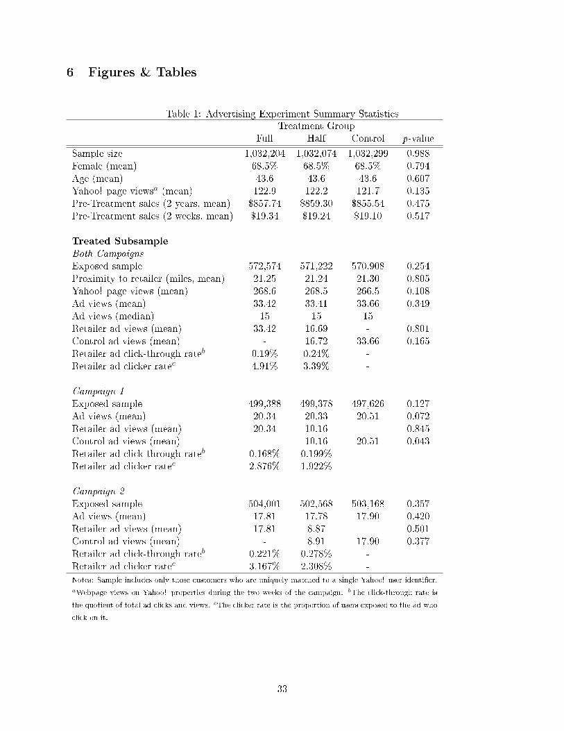
6 Figures & Tables

Table 1: Advertising Experiment Summary StatisticsTreatment Group

Full Half Control p-value

Sample size 1,032,204 1,032,074 1,032,299 0.988Female (mean) 68.5% 68.5% 68.5% 0.794Age (mean) 43.6 43.6 43.6 0.607Yahoo! page viewsa (mean) 122.9 122.2 121.7 0.135Pre-Treatment sales (2 years, mean) $857.74 $859.30 $855.54 0.475Pre-Treatment sales (2 weeks, mean) $19.34 $19.24 $19.10 0.517

Treated Subsample

Both Campaigns

Exposed sample 572,574 571,222 570,908 0.254Proximity to retailer (miles, mean) 21.25 21.24 21.30 0.805Yahoo! page views (mean) 268.6 268.5 266.5 0.108Ad views (mean) 33.42 33.41 33.66 0.349Ad views (median) 15 15 15Retailer ad views (mean) 33.42 16.69 - 0.801Control ad views (mean) - 16.72 33.66 0.165Retailer ad click-through rateb 0.19% 0.24% -Retailer ad clicker ratec 4.91% 3.39% -

Campaign 1

Exposed sample 499,388 499,378 497,626 0.127Ad views (mean) 20.34 20.33 20.51 0.072Retailer ad views (mean) 20.34 10.16 - 0.845Control ad views (mean) - 10.16 20.51 0.043Retailer ad click-through rateb 0.168% 0.199% -Retailer ad clicker ratec 2.876% 1.922% -

Campaign 2

Exposed sample 504,001 502,568 503,168 0.357Ad views (mean) 17.81 17.78 17.90 0.420Retailer ad views (mean) 17.81 8.87 - 0.501Control ad views (mean) - 8.91 17.90 0.377Retailer ad click-through rateb 0.221% 0.278% -Retailer ad clicker ratec 3.167% 2.308% -

Notes: Sample includes only those customers who are uniquely matched to a single Yahoo! user identi�er.

aWebpage views on Yahoo! properties during the two weeks of the campaign. bThe click-through rate is

the quotient of total ad clicks and views. cThe clicker rate is the proportion of users exposed to the ad who

click on it.

33

Table2:

E�ectof

Advertisingon

Sales:Re�nem

ents

inPrecision

(1)

(2)

(3)

(4)

(5)

(6)

(7)

Subsetof

Usersa

Everyone

Treated

Treated

Treated

Treated

Treated

Treated

Sales

After

First

AdExposureb

xx

xx

x

FullTreatment($)

0.673**

0.525**

0.559**

0.553**

0.535**

0.486**

0.477**

(0.317)

(0.237)

(0.217)

(0.217)

(0.213)

(0.204)

(0.204)

HalfTreatment($)

0.0248

0.189

0.307

0.307

0.239

0.241

0.221

(0.311)

(0.235)

(0.217)

(0.217)

(0.212)

(0.209)

(0.209)

Constant($)

15.52***

15.53***

13.17***

(0.122)

(0.166)

(0.154)

Covariates

Dem

ographicsc

xx

xx

Custom

ercategoriesd

xx

xPastsales(2

years)e

xx

Exposure

intensityf

x

Observations

3,096,577

1,714,704

1,714,704

1,714,704

1,714,704

1,714,704

1,714,704

R2

0.000

0.000

0.000

0.001

0.042

0.090

0.091

Robust

standard

errors

inparentheses.***p<0.01,**p<0.05,*p<0.1.aThetreatedofusers

are

those

whoare

exposedto

either

theretailer

or

thecontrolad.bSalesafter

�rstadexposure

modi�es

thetwo-weekexperim

ent'ssalesoutcometo

excludeallsalespriorto

auser's�rstexposure

toeither

theretailer

orcontrolad.cTwo-yearsalesofpre-treatm

ent�

both

onlineandin-store�attheweekly

levelexceptforaggregate

salesfor

weeks9through44and61through104.Formodelsthatuse

salesafter

the�rstadexposure

astheoutcomevariable,weincludesalesfrom

the

beginningofthecampaignto

that�rstexposure.dDem

ographic

covariatesincludeindividualgender,age,

state

dummiesaswellastheuser's

tenure

asaYahoo!customer.eTheretailer

customer

category

covariatesincludecategoricalvariablesforrecency

oflastpurchase,customer

loyalty,

andlifetimecustomer

spending.fTheexposure

intensity

covariatesinclude�xed

e�ects

fortheday

ofthe�rstadexposure

andthenumber

of

totalexposures(retailer

orcontrol)for1to

30separately

andasingleindicatorfor>30.

34

Table3:

Estim

ates

oftheE�ects

ofAdvertisingFrequency

(1)

(2)

(3)

(4)

(5)

(6)

DependentVariable

Sales

Sales

Sales

Sales

Sales

4-week

Sales

Subsetof

Usersa

0<θ≤

500<θ≤

500<θ≤

500<θ≤

500<θ≤

500<θ≤

50

β:Number

ofad-views,f

β̄=

0.0368***

0.0375***

0.0373***

0.0371***

0.0159

0.0612***

(0.0172)

(0.0128)

(0.0128)

(0.0102)

(0.0276)

(0.0158)

β:ad-viewssquared,f2

0.000626

(0.000750)

γθ,γ1Potential

Ad

Views,θ

50γ̂θ's

50γ̂θ's

-0.000302

(0.00993)

Constant

--

15.20***

15.19***

1.53***

31.24***

(0.152)

(0.125)

(0.530)

(0.193)

Observations

1,395,826

1,395,826

1,395,826

1,395,826

1,395,826

1,395,826

R-squared

0.000

0.000

0.000

0.000

0.000

0.000

Robust

standard

errors

inparentheses.***p<0.01,**p<0.05,*p<0.1.Allregressionswereperform

edonthesubsample

such

that0<θ≤

50

whereθisthetotalnumber

oftheretailer'sandcontroladim

pressionsseen

duringthetwo-weekcampaign.aSubsetofusers

are

those

whoare

exposedto

either

theretailer

orthecontrolad(Treated).

35

Table4:

HeterogenousTreatmentE�ects

byConsumer

Proxim

ityto

theRetailer

(1)

(2)

(3)

(4)

HeterogeneousE�ects

Variable

Distance

Recency

Monetary

Value

Income

Condition

Lives

within

1

mileofnearest

store

Transacted

in8

weeks

pre-treatm

ent

Spentover$1,000

in2years

pre-treatm

ent

Earns$100,000

ormore

Subsetof

Usersa

Treated

Treated

Treated

Treated

Sales

After

First

AdExposureb

xx

xx

`Near'in

FullTreatment

2.883**

1.624**

1.735*

0.810**

(1.430)

(0.752)

(0.933)

(0.332)

`Far'in

FullTreatment

0.485**

0.129

0.161

0.112

(0.233)

(0.139)

(0.103)

(0.240)

`Near'in

HalfTreatment

1.523

0.804

0.481

0.383

(1.528)

(0.776)

(0.959)

(0.339)

`Far'in

HalfTreatment

0.340

0.0485

0.156

0.0463

(0.240)

(0.138)

(0.102)

(0.242)

Covariates:

FullSetc

xx

xx

H0

:∆sales near<

∆sales far

Full:F-test(p-value)

0.049

0.025

0.047

0.045

Half:F-test(p-value)

0.222

0.169

0.368

0.210

Full&

Half:F-test(p-value)

0.064

0.037

0.051

0.059

%Non-m

issingcond.datad

77.1%

100%

100%

98.2%

Observations

1,714,704

1,714,704

1,714,704

1,714,704

R2

0.103

0.103

0.103

0.103

Estim

atesare

fortheaveragetreatm

ente�ectduringthetwoweeksoftheexperim

entconditionalontherelevantconsumer

characteristics.

Robust

standard

errors

inparentheses.***p<0.01,**p<0.05,*p<0.1.aThetreatedofusers

are

those

whoare

exposedto

either

theretailer

orthecontrolad.bSalesafter

�rstadexposure

modi�es

theoutcomemeasure

toexcludeallsalespriorto

auser's�rstexposure

toeither

the

retailer

orcontrolad.cIncludes

dem

ographics,customer

categories,two-yearofpast

sales,andexposure

intensity

(see

Table2fordetails).We

alsoincludeindicatorvariablesforthegiven

condition.dThedata

forsomevariables(distance,income,

gender)isincomplete.Weincludeall

observationshow

ever

astheseim

provetheestimatesforthecovariates.

36

Table 5: E�ects of the Advertising During and After the Campaign

(1) (2) (3)

TimeframeCampaign 1(1 week)

Campaign 2(1 week)

During & AfterCampaigns(4 weeks)

Subset of Usersa Treated Treated TreatedSales After First Ad Exposureb x x x

Full Treatment ($) 0.116 0.382** 0.525*(0.144) (0.153) (0.309)

Half Treatment ($) 0.059 0.156 0.363(0.141) (0.155) (0.312)

Covariates: Full Setc x x x

Observations 1,496,392 1,509,737 1,714,704R2 0.058 0.056 0.170

Robust standard errors in parentheses. *** p<0.01, ** p<0.05, * p<0.1. aThe treated of users are

those who are exposed to either the retailer or the control ad. bSales after �rst ad exposure modi�es the

outcome measure to exclude all sales prior to a user's �rst exposure to either the retailer or control ad.

cIncludes demographics, customer categories, two-year of past sales, and exposure intensity (see Table 2

for details). We also include indicator variables for the given condition.

Table 6: E�ects of the Advertising, Online versus In-Store

(1) (2) (3)

Dependent Variable (2 weeks) Total Sales In-Store Sales Online SalesSubset of Usersa Treated Treated TreatedSales After First Ad Exposureb x x x

Full Treatment ($) 0.477** 0.323* 0.154**(0.204) (0.172) (0.0779)

Half Treatment ($) 0.221 0.185 0.036(0.209) (0.176) (0.081)

Covariates: Full Setc x x x

Observations 1,714,704 1,714,704 1,714,704R2 0.091 0.078 0.135

Robust standard errors in parentheses. *** p<0.01, ** p<0.05, * p<0.1. aThe treated of users

are those who are exposed to either the retailer or the control ad. bSales after �rst ad exposure

modi�es the outcome measure to exclude all sales prior to a user's �rst exposure to either the

retailer or control ad. cIncludes demographics, customer categories, two-year of past sales, and

exposure intensity (see Table 2 for details). We also include indicator variables for the given

condition.

37

Table7:

E�ects

oftheAdvertising:

Probabilityof

Purchase,BasketSize,versusShoppingTrips

(1)

(2)

(3)

(4)

(5)

(6)

DependentVariable(2

weeks)

Sales

Probability

ofTransaction

Sales

Conditional

On

Transaction

ShoppingTrips

Online+

In-Store

ShoppingTrips

In-Store

ShoppingTrips

Online

Subsetof

Usersa

Treated

Treated

Transacted

Treated

Treated

Treated

Sales

After

First

AdExposureb

xx

xx

xx

FullTreatment($)

0.477**

0.000426

3.822

0.00196**

0.00129*

0.000662***

(0.204)

(0.000461)

(2.391)

(0.000795)

(0.000698)

(0.000212)

HalfTreatment($)

0.221

0.000474

1.365

0.001162

0.000956

0.000205

(0.209)

(0.000462)

(2.438)

(0.000793)

(0.000698)

(0.000211)

Covariates:FullSetc

xx

xx

xx

Observations

1,714,704

1,714,704

132,568

1,714,704

1,714,704

1,714,704

R2

0.091

0.147

0.107

0.174

0.171

0.090

Robust

standard

errors

inparentheses.***p<0.01,**p<0.05,*p<0.1.aThetreatedofusers

are

those

whoare

exposedto

either

theretailer

orthecontrolad.bSales

after

�rstadexposure

modi�es

theoutcomemeasure

toexcludeallsalespriorto

auser's�rstexposure

toeither

theretailer

orcontrolad.cIncludes

dem

ographics,customer

categories,two-yearofpast

sales,andexposure

intensity

(see

Table2fordetails).Wealsoincludeindicatorvariablesforthegiven

condition.

38

Figure 1: Histogram of Customers' Distance to the Nearest Store by Treatment Assignment

0

10,000

20,000

30,000

40,000

0 10 20 30 40 50Crow Flies Distance to Nearest Store (Miles)

Num

ber

of C

usto

mer

s

Treatment Assignment

Control

Half Treatment

Full Treatment

Figure 2: Histogram of Total Ad Exposures (Retailer and Control Ads)

0

100,000

200,000

300,000

400,000

500,000

0 20 40 60 80 100Number of Ad Exposures

Num

ber

of C

usto

mer

s

Treatment Assignment

Control

Half Treatment

Full Treatment

39

Figure 3: Histogram of Average Weekly Purchases During the Two Years Before the Experiment

0

50,000

100,000

150,000

200,000

250,000

300,000

$−20 $0 $20 $40 $60 $80 $100Average Weekly Sales: 2 Years Before Treatment

Num

ber

of C

usto

mer

s

Treatment Assignment

Control

Half Treatment

Full Treatment

Figure 4: Histogram Total Purchases by Transacting Customers During the Experiment

0

2,000

4,000

6,000

8,000

10,000

$−500 $0 $500 $1,000 $1,500 $2,000Total Sales: 2 Weeks Before Campaigns

Num

ber

of C

usto

mer

s

Treatment Assignment

Control

Half Treatment

Full Treatment

40

Figure 5: Histogram Total Purchases by Transacting Customers During the Experiment

0

2,000

4,000

6,000

8,000

10,000

$−500 $0 $500 $1,000 $1,500 $2,000Total Sales: 2 Weeks of Campaigns

Num

ber

of C

usto

mer

s

Treatment Assignment

Control

Half Treatment

Full Treatment

Figure 6: Indexed Sales Given a Customer's Experimental Ad Exposures (θ)

0.8

0.9

1.0

1.1

1.2

Rel

ativ

e S

ales

(T

o W

eekl

y M

ean)

0 10 20 30 40 50Potential Ad Views (Ad Type): q

Pre-Weeks 1-8Pre-Weeks 9-52Pre-Weeks 53-104

Pre-Weeks 1-104 (2 years)During 2-Week Campaign95% CI During

41

Figure 7: Marginal Impact of Ad Frequency Estimates βθ by Ad Type (θ)

-0.50

0.00

0.50

1.00

1.50

Sal

es Im

pact

($)

0 10 20 30 40 50

Potential Ad Views (Ad Type): q

Average Effect of Frequency95% Confidence Intervals

* Estimates obtained by regressing sales on ad views interacted with dummies for potential ad views (ad type), q<=50.

42

Figure 8: Joint Distribution of Retailer Ad Views (f) and Ad Type (θ)

0

10

20

30

40

50A

d V

iew

s: f

0 10 20 30 40 50Potential Ad Views (Ad Type): q

* The area of each square is proportional to the number of customers.

Figure 9: The E�ect of Advertising by Proximity in Grossman and Shapiro (1984)'s Model ofAdvertising in a Di�erentiated Market

ϕ(1-ϕ)

Proximity to Firm A

0 10.5

Effect of

Advertising

on Demand

ϕ2/2

43