RENEWABLE PORTFOLIO STANDARDS: KANSASRENEWABLE PORTFOLIO STANDARDS: KANSAS FINAL REPORT | FEBRUARY...

RENEWABLE PORTFOLIO STANDARDS:KANSASFINAL REPORT | FEBRUARY 2015

TYLER BROUGH PH.DUtah State University

KEN SIMStrata Policy

JACOB FISHBECKStrata Policy

RANDY T SIMMONS PH.DUtah State University

RYAN M. YONK, PH.DUtah State University

Institute of Political Economy, Utah State University | 1

RENEWABLE PORTFOLIO STANDARDS: KANSAS

PRIMARY INVESTIGATORS: Randy T Simmons, PhD Utah State University

Ryan M. Yonk, PhD Utah State University Tyler Brough, PhD Utah State University Ken Sim, MS Strata Policy Jacob Fishbeck Strata Policy

2 | Renewable Portfolio Standards: Kansas

TABLE OF CONTENTS

Table of Contents ............................................................................................................................. 2 Executive Summary ......................................................................................................................... 3

Background ................................................................................................................................. 3 Results ......................................................................................................................................... 5 Tax Analysis with STAMP ......................................................................................................... 5 Empirical Analysis ...................................................................................................................... 7 State Coincident Event Study ..................................................................................................... 7 The Structural Panel VAR-X Model ........................................................................................ 10 Conclusions from the Empirical Analysis ................................................................................ 11 Institutional Analysis ................................................................................................................ 11 Conclusion ................................................................................................................................ 13

Appendix A .................................................................................................................................... 14 Technical Considerations of the Beacon Hill Institute’s Study in Kansas ............................... 14 Ratepayer Effects ...................................................................................................................... 16 Modeling the Policy Using STAMP ......................................................................................... 17

Appendix B .................................................................................................................................... 20 Explanation of Empirical Study Methodology ......................................................................... 20

Appendix C .................................................................................................................................... 26 Graphical Analysis of the Dynamic Multiplier Analysis .......................................................... 26


EXECUTIVE SUMMARY

The U.S. has no federal mandate for “renewable” power production. Instead, a majority of states, including Kansas, have created their own state laws called Renewable Portfolio Standards (RPS). These laws mandate the presence of certain renewable sources among the overall menu of sources from which electricity companies produce power. This report analyzes how the changes in electricity markets caused by RPS alter the functioning of a state’s economy and institutions, with a specific focus on Kansas. Our report uses a tax-based model, an empirical analysis, and a survey of legal rules. The following are our key findings:

• Our tax analysis found that Kansas’ RPS will increase fiscal and economic costs significantly between now and 2020. During that period, Kansas electricity ratepayers will face $171 million in elevated electricity costs beyond what they would have paid in the absence of an RPS. In addition, RPS will cause significant macroeconomic repercussions, including the loss of 795 jobs, a decrease in investment of $14 million, and a decrease in personal disposable income of $72 million in 2020 alone. To obtain these results, we used a mature, robust, computable general equilibrium model, called STAMP (State Tax Analysis Modeling Program), developed by the Beacon Hill Institute at Suffolk University.

• Our empirical analysis suggests that the tax model is too modest. We discovered significant harmful effects on the economies of all states with RPS. States that have adopted an RPS have seen a drop in industrial electricity sales by almost 14 percent. Real personal income has fallen by almost four percent, which figures to a loss of $4.85 billion in 2013, or $4,367 less per family. Non-farm employment has declined by nearly 3 percent. Lastly, RPS is correlated with an increase of 10 percent in a state’s unemployment rate, equaling a loss of 5,500 jobs.

• Our analysis of the legal rules surrounding RPS in Kansas suggest that the regulatory climate is especially burdensome compared to most states we examined, making RPS an even worse venture for taxpayers than the tax-based or empirical analyses suggest.

BACKGROUND

One of the United States’ defining cultural and political initiatives of the past thirty years has been the push for renewable electricity generation and the abandonment of generation from fossil fuels. Kansas in particular has been working toward renewable wind energy since as early as 1999, when Westar Energy (then known as Westar Resources) built the first utility-scale wind


turbine production facility with the installation of two 600 kW Vestas wind turbines. An abundance of wind blows through the grasslands of the Midwest, making wind energy a desirable option for renewable energy advocates in that area. In fact, since 2008, at least one wind energy project has come online in Kansas every year. That timing correlates strongly with the implementation of the state’s Renewable Portfolio Standard.1

Governor Kathleen Sebelius was the state’s first real proponent for renewable energy and she laid the groundwork for the current RPS in Kansas. From 2007 to 2009, she instituted voluntary renewable energy standards, which encouraged the use of renewable energy but did not force energy companies to meet any mandates. In 2009, she began to push for mandatory renewable energy standards, feeling that her current voluntary policies were not doing enough to promote renewable energy.

Governor Mark Parkinson took up this mantle in May of 2009 when he signed H.B. 2369, the Renewable Energy Standards Act (RESA), creating legislation for a mandatory RPS in Kansas, thereafter known as Kansas’ Renewable Energy Standards (RES). The mandate required the following: Renewable energy sources must provide at least 10 percent of Kansas’ power generation between 2011 and 2015, 15 percent between 2016 and 2019, and 20 percent by 2020. Although many other states base renewable generation percentages on the share of total retail electric sales, Kansas’ RPS mandate is based upon generation capacity.

The mandate also provided a list of available technologies that qualify as renewable energy. That list includes wind, solar, landfill gas, current hydropower, new hydropower that is less than 10 megawatts (MW), and a variety of types of biomass. The RES also stipulate that if utilities do not abide by the RPS, they will be assessed a penalty equal to double the value of the Renewable Energy Credits (RECs) that would have been required for that year. That penalty can be increased as a punitive measure or decreased when utilities demonstrate good-will attempts at compliance. RECs are tradable commodities awarded for the production of 1 megawatt-hour (MWh) from a qualified renewable energy resource. They are proof that a utility company has achieved required levels of renewable energy production, and can be traded or stockpiled in times of excess production (production above the mandated RPS levels for that year). RECs remain valid for two years after their date of production, after which they are officially retired.2

States have sometimes resorted to other means of inducing renewable electricity generation, including by using existing energy or environmental regulations as leverage in bargaining for an RPS. In 2009—before Kansas’ RES went into effect—Sunflower Electric Company motioned their intent to build a coal-fired generating plant in Holcomb. They met resistance, however,

1 Polsinelli, & KEIN. (2014). Annual economic impacts of Kansas wind energy 2014 report. California: Alan Claus Anderson, Britton Gibson, Luke Hagedorn, Scott W. White. Retrieved from http://www.polsinelli.com/~/media/Articles%20by%20Attorneys/Anderson_Gibson_Hagedorn_Feb_2014 2 United States Department of Energy, 2014, op. cit.


from the Kansas Department of Health and Environment, which objected to the air pollution the plant would potentially create. Governor Parkinson, in his desire to establish an RPS in Kansas, reached an agreement with Sunflower Electric. The governor agreed to issue an air permit for the Holcomb plant, and in return Sunflower and the utility industry agreed to support expanded renewable energy initiatives.3 Even though Kansas has now effectively implemented its RES, the Holcomb plant has yet to be built.

Since its inception, the RES has not been overwhelmingly popular in Kansas, and eight separate attempts have been made to repeal it.4 Some of those attempts achieved greater acceptance in the state legislature, but ultimately each one failed. The most recent attempt was in May 2014 when a bill was introduced into the House which would end Kansas’ RPS through a gradual reduction. The bill narrowly lost in a vote of 63-60.5 Despite the failures, constituents continue to fight against the RPS, and many politicians are beginning to support phasing it out, including current Governor Sam Brownback.6

RESULTS

TAX ANALYSIS WITH STAMP

The Energy Information Association (EIA) calculates the Levelized Avoided Costs of Electricity (LACE)—a number designed to provide direct, accurate cost comparisons between conventional power sources and distributed (localized) power sources, such as wind and solar. Using this information from, we were able to calculate an estimated net cost of the RES. By using state specific reporting we are able to estimate the amount of renewable energy that would be mandated due to the law, and the associated economic effects. Appendix A explains the methodology in detail. Table 1 displays the cost estimates and economic impact of the current RES in 2020.

3 Kansas Electric Power Cooperative, Inc. (2009). 2009 annual report. Retrieved from http://pbadupws.nrc.gov/docs/ML1012/ML101260216.pdf 4 Barnett, D. (2014). Capital gains. Climate + Energy Project. Retrieved from http://climateandenergy.org/news.1050012.capital-gains 5 Lowry, B. (2014a). Kansas House rejects repeal of renewable energy standards. The Wichita Eagle. Retrieved from http://www.kansas.com/news/politics-government/article1141897.html 6 Lowry, B. (2014b). Next legislative session could be end for Kansas’ renewable energy standard. The Wichita Eagle. Retrieved from http://www.kansas.com/news/politics-government/article4202126.html


TABLE 1: THE COST OF THE RES ON KANSAS IN 2020

Costs Estimates (2012 $) Expected Value Total Net Cost in 2020 $54 million Total Net Cost 2015-2020 $171 million Electricity Price Increase in 2020 (cents per kWh) .11 cents Percentage Increase (%) 1.13% Economic Indicators Total Employment (jobs) -795 Investment -$14 million Real Disposable Income -72 million

The current RES is expected to impose net costs of $54 million in 2020 as a result of electricity prices increasing by an expected 0.11 cents per kilowatt-hour (kWh), or by 1.13 percent. The RES will cost Kansas’ electricity customers $171 million from 2015 to 2020, with 2020 being the final year of increases.

The STAMP model simulations indicate that, upon full implementation, the RES is likely to hurt Kansas’ economy. The state’s ratepayers will likely face higher electricity prices that will increase their cost of living, which will in turn put downward pressure on households’ disposable income. By 2020, Kansas’ state economy will have 795 fewer total jobs. This includes jobs created in the renewable energy sector as well as jobs lost due to higher electricity costs and dynamic spending decreases.

The job losses and price increases will reduce real incomes as firms, households, and governments spend more of their budgets on electricity and less on other items, such as home goods and services. In 2020, real disposable income will fall by an expected $72 million. Furthermore, net investment will fall by $14 million. Table 2 shows how the RES is expected to affect the average annual electricity bills of households and businesses in Kansas. In 2020, the RES is expected to cost families an additional $15 per year; commercial businesses $75 per year; and industrial businesses $440 per year. Over the entire period from 2015 to 2020, the RES will cost families an additional $50; commercial businesses $240; and industrial businesses $1,420.

TABLE 2: ANNUAL EFFECTS OF THE RES ON KANSAS ELECTRICITY RATEPAYERS

Estimates (2012 $) Expected Value Cost in 2020 Residential Ratepayer $15 Commercial Ratepayer $75 Industrial Ratepayer $440 Cost over period (2015-2020) Residential Ratepayer $50 Commercial Ratepayer $240 Industrial Ratepayer $1,420


EMPIRICAL ANALYSIS

STATE COINCIDENT EVENT STUDY

In this section, we present the results of an event study for state coincident indices—a methodology first fashioned by the Federal Reserve Bank of Philadelphia.7 The event study indexes the economic conditions of all states across multiple points in time, and assigns as “point zero” each state’s economic conditions on the dates of their respective RPS implementations. The study then compares said economic conditions over a span of 48 months before to 48 months after that enactment date. We then average the results across the different states, which, given that RPS have been implemented in states over a long period, should minimize the effects of anomalies such as recessions and the enactment of other energy-related laws. The indices of each state RPS policy, while enacted in a different calendar month and year, can thus be lined up in this so-called “event time” and averaged. For these reasons, the event study has become a time-honored empirical methodology in finance and economics and a standard course of analysis for the Philadelphia Fed. It is a simple but powerful method for measuring the effect of an exogenous shock to an economic variable of interest. See Mackinlay for a more in-depth discussion of the event study methodology.8 Table 3 presents the dates of 31 different states that have enacted an RPS policy.

7 Federal Reserve Bank of Philadelphia. (2015, January 29). State coincident indexes. Retrieved from http://www.philadelphiafed.org/research-and-data/regional-economy/indexes/coincident/ 8 MacKinlay, A.C. (1997). Event studies in economics and finance. Journal of Economic Literature, 35(1), 13-39.


TABLE 3: THE DATES (MONTH AND YEAR) OF THE 31 STATES THAT HAVE ENACTED AN RPS POLICY TO DATE

State RPS Enactment Date Arizona July, 2007 California January, 2003 Colorado December, 2004 Connecticut July, 1998 Delaware July, 2005 Hawaii December, 2003 Iowa January, 1983 Illinois August, 2007 Kansas July, 2009 Massachusetts April, 2002 Maryland January, 2004 Maine March, 2000 Michigan October, 2008 Minnesota February, 2007 Missouri November, 2008 Montana April, 2005 North Carolina January, 2008 New Hampshire July, 2007 New Jersey September, 2001 New Mexico September, 2007 Nevada January, 1997 New York September, 2004 Ohio May, 2008 Oregon January, 2007 Pennsylvania February, 2005 Rhode Island June, 2004 South Carolina June, 2014 Texas September, 1999 Washington November, 2006 Wisconsin December, 2001 West Virginia July, 2009


The results of the event study are presented in Figure 1, wherein we see the response of the state coincident index to the enactment of RPS policies. The coincident index is a measure of the strength of a state economy.

FIGURE 1: THE RESPONSE OF THE STATE COINCIDENT INDEX TO THE ENACTMENT OF RPS POLICIES.

The horizontal axis shows months before and after point zero (RPS enactment). The vertical axis shows an indexed scale measuring the average reaction of states in terms of several economic indicators.

As can be seen in Figure 1, the average effect on the state coincident index is a precipitous drop surrounding the enactment of an RPS policy. This evidence is suggestive of a negative effect of an RPS policy on a state economy. While suggestive, the evidence from the event study warrants further exploration into the effects, since state economies also appear to decline several months prior to the enactment of an RPS. The next section presents the structural panel VAR-X model, which provides further evidence of the negative economic effects of an RPS.


THE STRUCTURAL PANEL VAR-X MODEL

The VAR model takes into account the nature of the state macroeconomic variables that could provide unwanted feedback into the model, and considers their dynamic interactions. By including a panel dimension to the model we can include the data for multiple states in a single model. We include fixed effects to control for state-level heterogeneity. We impose a recursive causal ordering on the VAR-X model to allow for structural interpretation of dynamic multiplier analysis of the RPS policy variable. Table 4 presents the cumulative effects of an RPS on the state economy via structural policy simulations.

TABLE 4: THE LONG-RUN EFFECTS ON STATE MACROECONOMIC VARIABLES

State Economic Variable Long-Run Effect Electricity Sales -13.7075% Real Personal Income -3.6369% Non-farm Employment -2.8416% Manufacturing Employment 3.7454% Unemployment Rate 9.6841%

The cumulative effect of the enactment of an RPS policy on state electricity sales is a staggering 13.7-percent decline. This is, perhaps, not surprising as the RPS increases the cost of electricity generation. Real personal income declines in the long run by 3.6369 percent, which figures to a loss of $4.85 billion in 2013, or $4,367 less per family.9 Non-farm employment declines in the long run by 2.8 percent. Only one analyzed component of non-farm employment, manufacturing employment, does not experience a long-term suppression in response to an RPS policy, although as we see in the graphical analysis, it does still experience a sharp decline in the short term. Most significantly, the state unemployment rate increases by 9.6 percent. This means that, at the end of last year, Kansas had 5,500 fewer jobs than it would have had without the RPS.10 There can be no doubt that the combined economic effect on an RPS enactment, as measured by the structural panel VAR-X model, is a severe decline in the Kansas economy. A graphical representation of the analysis, showing the changes over time that lead to these results, can be found in Appendix C.

9 Bureau of Economic Analysis. (n.d.). Regional Data, Annual State Personal Income and Employment. Retrieved from http://www.bea.gov/iTable/iTable.cfm?reqid=70&step=1&isuri=1&acrdn=1#reqid=70&step=1&isuri=1 10 Bureau of Labor Statistics. (n.d.). Kansas. Retrieved from http://www.bls.gov/regions/mountain-plains/kansas.htm


CONCLUSIONS FROM THE EMPIRICAL ANALYSIS

We demonstrate strong empirical evidence that a Renewable Portfolio Standard has a lasting negative effect on a state economy. We present this evidence from both an event study of the state coincident index as measured by the Federal Reserve Bank of Philadelphia, as well as from structural policy simulations from a panel VAR-X model. The long-run effect of an RPS on state industrial production, as measured by electricity sales, is greater than a 13-percent decline. Real personal income declines in the long run after an RPS by almost 4 percent. The cumulative effect of an RPS on non-farm employment is nearly 3 percent. While the effect of an RPS on manufacturing employment is not as severe in the long run, it too demonstrates initial sharp declines lasting for several years. Finally, the state unemployment rate increases in the long run in response to an RPS by nearly 10 percent. These are strong and lasting effects in 4 of the 5 variables measuring the state economy. The combined econometric evidence makes clear that an RPS policy has a severely negative economic effect on a state that enacts such.

INSTITUTIONAL ANALYSIS

Our institutional analysis provides a detailed account of all the regulations that create barriers for the state, electricity generators, and utilities to comply with an RPS. We find several instances in the regulatory structure of Kansas’ RPS that could be reasonably expected to hinder mere compliance with the law.

Kansas’ Renewable Energy Standard (RES) mandates that 20 percent of peak demand capacity must be supplied from renewable sources by 2020. This approach is not typical, as most states base their RPS benchmarks on total electricity retail sales. Generation capacity, which is generally the “gross capacity owned or leased by a utility less the auxiliary power used to operate [their] facilities,”11 is tedious to determine. Doing so requires a four-hour test of a generator, which must be free of “[limitations] on performance due to ambient conditions, equipment, or operating or regulatory restrictions.”12 If the facility is not tested for the entire duration under these conditions, the test results are still used anyway. They are simply considered, by extrapolation, to represent an accurate test under correct conditions. The same is true for multi-unit facilities, such as wind farms, except now the capacity of 10 percent of the wind turbines will be considered representative of all turbines in the same farm. Additionally, if the testing of a particular generator is impractical, then the “nameplate” capacity, as purported by the

11 DSIRE. (2014, December 31). Renewable Energy Standards. Retrieved from http://www.dsireusa.org/incentives/incentive.cfm?Incentive_Code=KS07R&re=0&ee=0 12 Electric Utility Renewable Energy Standard, 2014 Supplement to the Kansas Administrative Regulations 82-16-1. (2014, January). Retrieved from http://www.sos.ks.gov/pubs/KAR/2014/2014_KAR_Supplement_Book_1.pdf


manufacturer, will be used as a stand-in. The tested capacity of a generator is unlikely ever to exceed the capacity purported by the manufacturer—which is inherently disposed to convey an inflated number—and since the generator’s compliance benchmarks will be based thereon, this could cause power providers to overproduce.13

Such extrapolation could be problematic for utilities precisely because compliance benchmarks are based on generation capacity. If compliance were based on total electricity retail sales, then a utility would know exactly how many renewable facilities, and of what capacity, to build in order to satisfy their requirements. A faulty test of a particular generator, however, could handicap a utility by tricking it into building too much or too little generation capacity and/or creating a perpetual shortage or excess of power.

RES-eligible sources include wind, solar thermal, solar photovoltaic, dedicated crops grown for energy production, cellulosic agricultural residues, plant residues, methane from landfills or wastewater treatment, clean and untreated wood products, existing hydropower, new hydropower of no more than 10 MW, fuel cells using hydrogen, and other sources of energy that become available. Kansas’ RES also allows for net metering.

Generators and utilities can still buy and sell Renewable Energy Certificates (RECs) in the state of Kansas, but the amount of electrical production the REC conveys must be converted, using a complex formula, so that it can comport with the generating capacity of the buyer. This will prevent a buyer from purchasing an REC from another generator with a disproportionately high capacity, so as to escape its own obligations. If a buyer does not have a facility of the same resource as the original seller, then the capacity of the buyer’s overall renewable energy generation is used, and if that number is unavailable, a default capacity factor of 34 percent is the used. RECs in Kansas are valid for only two years after generation—an unusually short period, compared with other states.

Unlike other states, older renewable technologies can be eligible to generate RECs for complying with the RES, but Kansas does significantly favor newly installed technologies over old ones. Each MW of eligible capacity installed in Kansas after January 1, 2000, counts as 1.1 MW for the purpose of compliance, amounting to a 10-percent reward for generators who have newer facilities.

Failing to meet the renewable energy standard results in a fine that is equal to twice the market value of the RECs that would have been required to meet that year’s requirement. Penalties may be increased or decreased upon evaluation. Utilities are exempt from administrative penalties if the retail rate impact is one percent or more.

13 Ibid.


Even in judging an RPS on its own terms, and assuming that all potential economic and environmental ramifications are acceptable, the legal and regulatory structure behind RPS makes compliance itself a difficult task; this fact does not change even in spite of the good-faith efforts made by utilities. Proponents of RPS often gloss over these considerations and assume that the mere presence of a law is solely required to effect their desired outcome. Our analysis clearly demonstrates that reality is more complicated.

CONCLUSION

The evidence from these three studies paints a clear picture about the effects of RPS. Our tax analysis with STAMP found that Kansas’ RPS will increase fiscal and economic costs significantly between now and 2020. These costs include a $171-million burden on Kansas electricity ratepayers, a loss of 795 jobs, a decrease in state investment by $14 million, and a decrease in personal disposable income of $72 million in 2020 alone. Our empirical analysis more than corroborates these predictions, finding a drop in industrial electricity sales in RPS states by almost 14 percent, real personal income by almost 4 percent, non-farm employment by nearly 3 percent, and an increase of 10 percent in the unemployment rate, which for Kansas means the state had 5,500 fewer jobs at the end of 2014 than they would have had without the RPS. While individual conditions in Kansas may allow for some variability in these actual figures, the overall finding is that long-run economic conditions in states with implemented RPS programs experience significant negative impacts. Our institutional analysis further describes the barriers that make it difficult for utilities to comply and for bureaucracies to enforce the RPS, finding that Kansas’ generation capacity scheme of compliance benchmarking produces manifest difficulties in compliance and enforcement. Any state currently deliberating on implementing a new RPS, or strengthening an existing one, should heed the results of these analyses as a warning of their harmful effects. Finally, states should refrain from following the fad of enacting such costly regulations, in spite of the policy’s political palpability or expediency.


APPENDIX A

TECHNICAL CONSIDERATIONS OF THE BEACON HILL INSTITUTE’S STUDY IN KANSAS

Authored by the Beacon Hill Institute at Suffolk University

This study utilized EIA projections to calculate the net effect to electricity prices due to the Kansas RES. Based on this design we were then able to simulate these changes in the STAMP model to measure the dynamic effects on the state economy.

The first step in this process was to calculate the amount of Megawatts (MW) of capacity that would be subject to the Kansas RES. Utilizing the Kansas Corporation Commission’s Report on Electric Supply and Demand we were able to calculate the ‘Total System Peak Load’ for the three major Investor Owned Utilities (IOU) and three major Cooperatives (Coop), for all years, municipal utilities which are included in the report are not required to follow the RES, therefore were not included.14 The average of the prior three years multiplied by that years requirement percent is the amount of generation required to come from eligible renewable sources.

The amount required to come from eligible renewable sources is not the actual amount of renewable sources that will be used to meet the requirement. One MW of in-state generation counts for 1.1 MWs in terms of satisfying the RES. In Appendix B of the Report on Electric Supply and Demand details of Renewable Capacity are supplied (which does not include instate multiplier), as well as the Total Renewable Capacity (which does include instate multiplier).15 Based on this difference we are able to interpolate the amount of MWs that are receiving the instate multiplier, while expanding this exercise for all IOUs and Coops allows us to determine the share of renewables that are in state for the duration of our projection. This means that the actual MW required are less than the calculation of the average three years peak load times the year’s requirement.

The level of renewable generation that would have come online without the policy under review, would not be attributed to the RES policy. The difference between this baseline and the amount of renewable energy need to satisfy the RES is the amount of renewable energy that has to come online due to the policy itself. The baseline level of renewables was set equal to the total amount of renewable generation in at the start of 2008, as the policy was introduced in 2009, then grown annually according to the projected growth of renewables generating capacity in the region per

14 Kansas Corporation Commission Report on Electric Supply and Demand, 2014. Retrieved from http://www.kcc.state.ks.us/pi/2014_electric_supply_and_demand_report.pdf. 15 Ibid., 15.


the AEO2008.1617 Some of these baseline renewables are part of municipal utilities, which are not considered as part of this study as they were not legally subject to the RES. We were unable to find any details on what this break down might be, so we assumed that share for municipal utilities was the same as their share of total system capacity.

The second data point calculated was the distribution of new renewable generation that came online due to the policy. The share of new renewable generation capacity was calculated based on several data points. The electricity generation projections minus baseline resulted in the required new renewable energy that would have to come online due to the RPS law. This amount was attributed to the various eligible renewable energies based on annual projections of renewable energy sources. Utilizing the AEO2014, we know the current distribution of energy sources in the state of Kansas, as well as projections though 2030 for the Southwest Power Pool/North, which is made up mostly of Kansas.18 Utilizing these projections, we used the ratio of future renewable energy sources as the dispersion of renewable energy sources that would meet the RPS.

Table 3: Projected Electricity Sales, Renewable Sales

Year Peak Load, MW Projected Baseline Renewable, MW RPS Requirement, MW

2015 9,328 715 903 2016 9,345 715 1,365 2017 9,444 715 1,395 2018 9,550 715 1,406 2019 9,628 715 1,417 2020 9,715 715 1,908

Now knowing the amount of renewable generation capacity that came online due to the RES the next step was to determine what types of renewable generation would be used to meet that

16 Energy Information Administration. (2014, May 1b). Kansas Electricity Profile 2012, table 4: Electric power industry capability by primary energy source, 1990-2012. Retrieved from http://www.eia.gov/electricity/state/kansas/. 17 Energy Information Administration. (2008, June). table 87: Renewable energy generation by fuel. http://www.eia.gov/oiaf/archive/aeo08/supplement/index.htm 18 Energy Information Administration, (2014, May 7b), op. cit.


requirement and how many megawatt hours (MWh) that would provide to the Kansas grid. Again using the AEO2014 we knew the breakdown of current renewable generation in the state, and we knew the expected growth rate of renewable capacity in the region, the Southwest Power Pool/North, which we use as a proxy for Kansas. We use the resulting ratio of renewable generation as the ratio of renewable generation that will be used to meet the RES, of which almost 100 percent is wind power with some biomass and hydroelectricity. The result of this calculation is the amount of MW capacity of different renewables that came online due to the policy being studies.

This MW capacity was then converted to the expected amount of MWh that would be produced by these renewable sources. In the AEO2014 it projects wind to have an approximate capacity factor of 0.40 during the range of our study, which we utilize. This is a favorable level compared to what is seen in actual generation according to EIA records.19 This combination results in the amount of MWh that will be provided from 2015 till 2020 by wind, hydro and biomass due to the RES.

With this calculation in place, we looked at the cost to provide a MWh of each type of renewable energy, or the Levelized Cost of Electricity (LCOE) versus the value of that MWh, or the Levelized Avoided Cost of Electricity (LACE).20 Using annual projections of the Southwest Powerpool / North LCOE and LACE Reference case we were able to determine the economic value of the proposal. The biomass and hydroelectricity LACE numbers were only presented for 2017 onwards. To complete our study we needed data for the years 2015 and 2016. To approximate the avoided cost in these years we calculated the annual growth rate displayed in the data for years 2017 through 2030 and worked backwards. For example, biomass in 2017 has a LACE of 60.03, increasing to 72.16 in 2030, or a 1.4 percent annual growth rate. The outcome of this calculation had us utilizing a rate of 59.17 in 2016 and 58.33 in 2015. This change had very minor effects on the results due to the fact that wind makes up such a large share of power due to the RES, which had all required data points. The total cost of the policy divided by the amount of electricity consumed in the state yields a percent cost of the policy.

RATEPAYER EFFECTS

To calculate the effect of the policy on electricity ratepayers, we used EIA data on the average monthly electricity consumption by type of customer: residential, commercial and industrial.21

19 Energy Information Administration. (2015, February 2). Form EIA-923 detailed data. Retrieved from http://www.eia.gov/electricity/data/eia923/ 20 Energy Information Administration. (n.d.). Assessing the economic value of new utility-scale electricity generation projects. Retrieved from http://www.eia.gov/renewable/workshop/gencosts/pdf/lace-lcoe_070213.pdf 21 U.S. Energy Information Administration, (2013, November 8), op. cit.


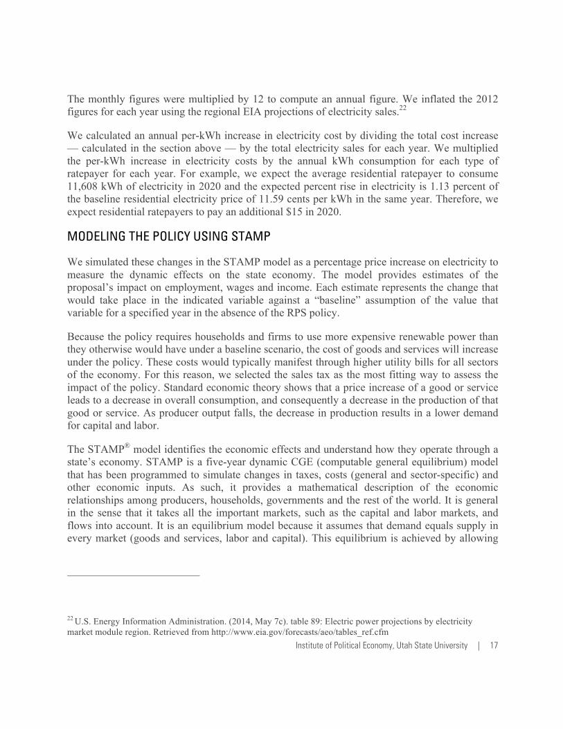
The monthly figures were multiplied by 12 to compute an annual figure. We inflated the 2012 figures for each year using the regional EIA projections of electricity sales.22

We calculated an annual per-kWh increase in electricity cost by dividing the total cost increase — calculated in the section above — by the total electricity sales for each year. We multiplied the per-kWh increase in electricity costs by the annual kWh consumption for each type of ratepayer for each year. For example, we expect the average residential ratepayer to consume 11,608 kWh of electricity in 2020 and the expected percent rise in electricity is 1.13 percent of the baseline residential electricity price of 11.59 cents per kWh in the same year. Therefore, we expect residential ratepayers to pay an additional $15 in 2020.

MODELING THE POLICY USING STAMP

We simulated these changes in the STAMP model as a percentage price increase on electricity to measure the dynamic effects on the state economy. The model provides estimates of the proposal’s impact on employment, wages and income. Each estimate represents the change that would take place in the indicated variable against a “baseline” assumption of the value that variable for a specified year in the absence of the RPS policy.

Because the policy requires households and firms to use more expensive renewable power than they otherwise would have under a baseline scenario, the cost of goods and services will increase under the policy. These costs would typically manifest through higher utility bills for all sectors of the economy. For this reason, we selected the sales tax as the most fitting way to assess the impact of the policy. Standard economic theory shows that a price increase of a good or service leads to a decrease in overall consumption, and consequently a decrease in the production of that good or service. As producer output falls, the decrease in production results in a lower demand for capital and labor.

The STAMP® model identifies the economic effects and understand how they operate through a state’s economy. STAMP is a five-year dynamic CGE (computable general equilibrium) model that has been programmed to simulate changes in taxes, costs (general and sector-specific) and other economic inputs. As such, it provides a mathematical description of the economic relationships among producers, households, governments and the rest of the world. It is general in the sense that it takes all the important markets, such as the capital and labor markets, and flows into account. It is an equilibrium model because it assumes that demand equals supply in every market (goods and services, labor and capital). This equilibrium is achieved by allowing

22 U.S. Energy Information Administration. (2014, May 7c). table 89: Electric power projections by electricity market module region. Retrieved from http://www.eia.gov/forecasts/aeo/tables_ref.cfm


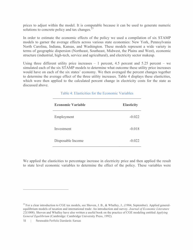
prices to adjust within the model. It is computable because it can be used to generate numeric solutions to concrete policy and tax changes.23

In order to estimate the economic effects of the policy we used a compilation of six STAMP models to garner the average effects across various state economies: New York, Pennsylvania North Carolina, Indiana, Kansas, and Washington. These models represent a wide variety in terms of geographic dispersion (Northeast, Southeast, Midwest, the Plains and West), economic structure (industrial, high-tech, service and agricultural), and electricity sector makeup.

Using three different utility price increases – 1 percent, 4.5 percent and 5.25 percent – we simulated each of the six STAMP models to determine what outcome these utility price increases would have on each of the six states’ economy. We then averaged the percent changes together to determine the average effect of the three utility increases. Table 4 displays these elasticities, which were then applied to the calculated percent change in electricity costs for the state as discussed above.

Table 4: Elasticities for the Economic Variables

Economic Variable Elasticity

Employment -0.022

Investment -0.018

Disposable Income -0.022

We applied the elasticities to percentage increase in electricity price and then applied the result to state level economic variables to determine the effect of the policy. These variables were

23 For a clear introduction to CGE tax models, see Shoven, J. B., & Whalley, J., (1984, September). Applied general-equilibrium models of taxation and international trade: An introduction and survey. Journal of Economic Literature 22(1008). Shoven and Whalley have also written a useful book on the practice of CGE modeling entitled Applying General Equilibrium (Cambridge: Cambridge University Press, 1992).


gathered from the Bureau of Economic Analysis Regional and National Economic Accounts as well as the Bureau of Labor Statistics Current Employment Statistics.24

24 For employment, see the following: U.S. Bureau of Labor Statistics. (n.d.). State and metro area employment, hours, & earnings. Retrieved from http://bls.gov/sae/. Private, government and total payroll employment figures for Michigan were used. For investment, see U.S. Bureau of Economic Analysis. (n.d.). National income and product account tables. Retrieved from http://www.bea.gov/itable/. See also BEA. (n.d.). Gross domestic product by state. Retrieved from http://www.bea.gov/regional/. We took the state’s share of national GDP as a proxy to estimate investment at the state level. For state disposable personal income, see BEA. (n.d.). State disposable personal income summary. Retrieved from http://www.bea.gov/regional/.


APPENDIX B

EXPLANATION OF EMPIRICAL STUDY METHODOLOGY

Methodology Constructed by Tyler Brough, Ph. D.

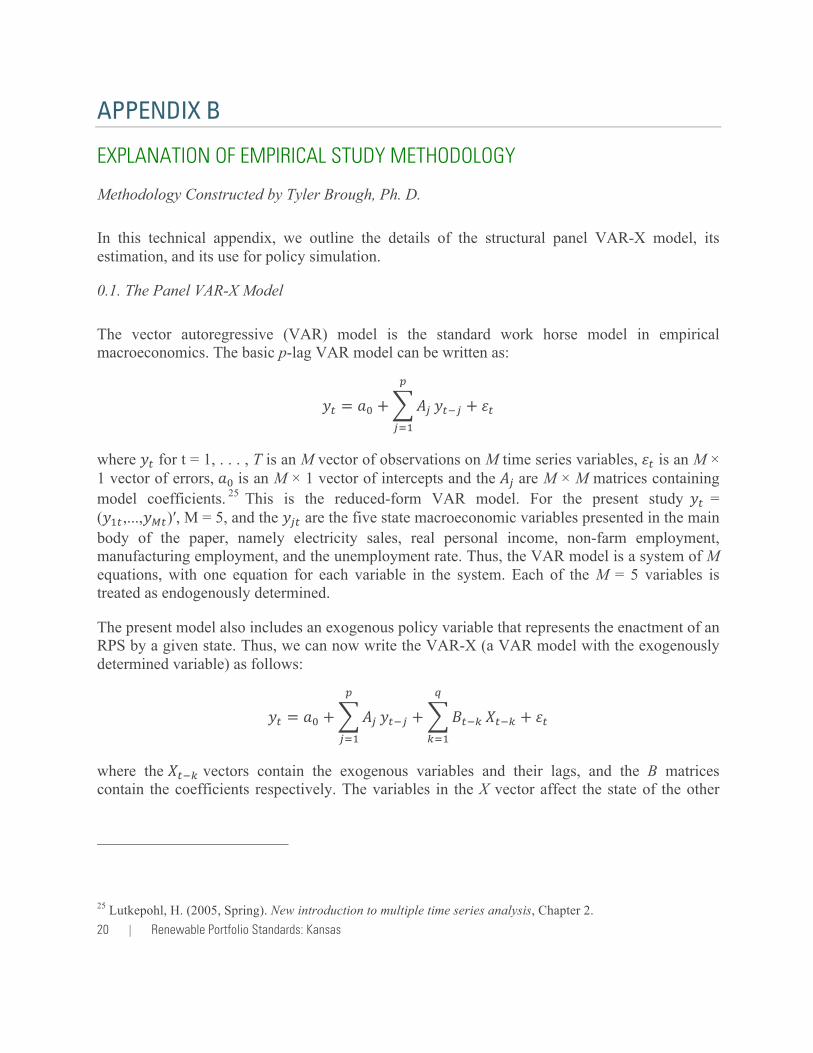
In this technical appendix, we outline the details of the structural panel VAR-X model, its estimation, and its use for policy simulation.

0.1. The Panel VAR-X Model

The vector autoregressive (VAR) model is the standard work horse model in empirical macroeconomics. The basic p-lag VAR model can be written as:

𝑦! = 𝑎! + 𝐴!

!

!!!

𝑦!!! + 𝜀!

where 𝑦! for t = 1, . . . , T is an M vector of observations on M time series variables, 𝜀! is an M × 1 vector of errors, 𝑎! is an M × 1 vector of intercepts and the 𝐴! are M × M matrices containing model coefficients. 25 This is the reduced-form VAR model. For the present study 𝑦! = (𝑦!!,...,𝑦!")′, M = 5, and the 𝑦!" are the five state macroeconomic variables presented in the main body of the paper, namely electricity sales, real personal income, non-farm employment, manufacturing employment, and the unemployment rate. Thus, the VAR model is a system of M equations, with one equation for each variable in the system. Each of the M = 5 variables is treated as endogenously determined.

The present model also includes an exogenous policy variable that represents the enactment of an RPS by a given state. Thus, we can now write the VAR-X (a VAR model with the exogenously determined variable) as follows:

𝑦! = 𝑎! + 𝐴!

!

!!!

𝑦!!! + 𝐵!!!

!

!!!

𝑋!!! + 𝜀!

where the 𝑋!!! vectors contain the exogenous variables and their lags, and the B matrices contain the coefficients respectively. The variables in the X vector affect the state of the other

25 Lutkepohl, H. (2005, Spring). New introduction to multiple time series analysis, Chapter 2.


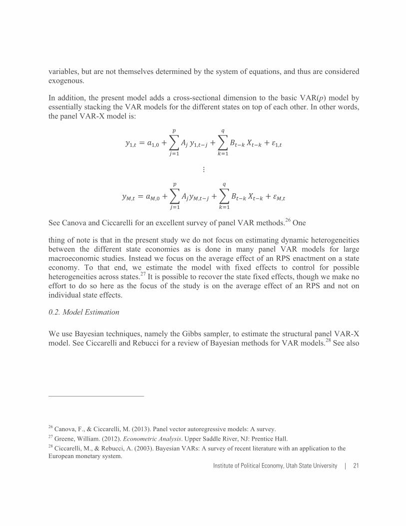
variables, but are not themselves determined by the system of equations, and thus are considered exogenous.

In addition, the present model adds a cross-sectional dimension to the basic VAR(p) model by essentially stacking the VAR models for the different states on top of each other. In other words, the panel VAR-X model is:

𝑦!,! = 𝑎!,! + 𝐴!

!

!!!

𝑦!,!!! + 𝐵!!!

!

!!!

𝑋!!! + 𝜀!,!

⋮

𝑦!,! = 𝑎!,! + 𝐴!𝑦!,!!!

!

!!!

+ 𝐵!!!

!

!!!

𝑋!!! + 𝜀!,!

See Canova and Ciccarelli for an excellent survey of panel VAR methods.26 One

thing of note is that in the present study we do not focus on estimating dynamic heterogeneities between the different state economies as is done in many panel VAR models for large macroeconomic studies. Instead we focus on the average effect of an RPS enactment on a state economy. To that end, we estimate the model with fixed effects to control for possible heterogeneities across states.27 It is possible to recover the state fixed effects, though we make no effort to do so here as the focus of the study is on the average effect of an RPS and not on individual state effects.

0.2. Model Estimation

We use Bayesian techniques, namely the Gibbs sampler, to estimate the structural panel VAR-X model. See Ciccarelli and Rebucci for a review of Bayesian methods for VAR models.28 See also

26 Canova, F., & Ciccarelli, M. (2013). Panel vector autoregressive models: A survey. 27 Greene, William. (2012). Econometric Analysis. Upper Saddle River, NJ: Prentice Hall. 28 Ciccarelli, M., & Rebucci, A. (2003). Bayesian VARs: A survey of recent literature with an application to the European monetary system.


Ocampo and Rodr ́ıguez for a very practical tutorial.29 We follow their Algorithm 3 for Bayesian estimation, which for simplicity we reproduce below.

Algorithm 1 Bayesian Estimation

Select the specification for the reduced form VAR-X, that is to choose values of p (endogenous variables lags) and q (exogenous variables lags) such that the residuals of the VAR-X (𝜀) have white noise properties. With this the following variables are obtained: T, p, q, k, where:

𝑘 = 1+ 𝑛𝑝 +𝑚(𝑞 + 1)

Calculate the values of Γ, S with the data (Y , Z) as:

Γ = (𝑍!𝑍)!!𝑍′𝑌 𝑆 = (𝑌 − 𝑍Γ)′(𝑌 − 𝑍Γ)

Generate a draw for matrix Σ from an inverse Wishart distribution with parameter S and T − k degrees of freedom.

Σ~𝑖𝑊!"#(𝑆,𝑇 − 𝑘)

Generate a draw for matrix Γ from a multivariate normal distribution with mean Γ and covariance matrix Σ (𝑍!𝑍)!!

Γ|Σ~𝑀𝑁!"#(Γ, Σ⨂ 𝑍!𝑍 !!)

Repeat steps 2-3 as many times as desired, save the values of each draw.

The draws generated can be used to compute moments of the parameters. For every draw the corresponding structural parameters, impulse response functions, etc. can be computed, then their moments and statistics can also be computed. The algorithm for generating draws for the inverse Wishart and multivariate normal distributions are presented in Bauwens et al., Appendix B.30

29 Ocampo, S., & Rodríguez, N. (2012). An introductory review of a structural VAR-X estimation and applications. Revista Colombiana de Estadística, 3, 479-508. 30 Bauwens, L., Lubrano, M., & Jean-Francois, R. (2000). Bayesian inference in dynamic econometric models. Oxford, UK: Oxford University Press.


Observe that in this notation:

Y =

y '1!y 't!y 'T

!

"

#######

$

%

&&&&&&&

,

Z =

1 y '0 ! y '1−p x '1"1 y 't−1 ! y 't−p x 't"1 y 'T−1 ! y 'T−p x 'T

"

#

$$$$$$$

%

&

'''''''

,

E =

ε '1!ε 't!ε 'T

!

"

#######

$

%

&&&&&&&

and finally,

Γ = v A1 … Ap B0 ! Bq"#$

%&'

Then the VAR-X model can be written simple as


𝑌 = 𝑍Γ+ 𝐸

We set 𝑝 = 3 and 𝑞 = 1 for simplicity.

0.3. Dynamic Multiplier Analysis

During the Gibbs sampling simulation, which we run for 5, 000 replications with 500 burn-in steps, we also conduct dynamic multiplier analysis for the exogenous RPS policy variable. We follow Algorithm 2 in Ocampo and Rodrıguez to conduct this analysis.31 This algorithm is as follows:

Algorithm 2 Identification by Long-Run Restrictions

Estimate the reduced form of the VAR-X model.

Calculate the VMA-X representation of the model (matrices 𝛙!) and the convariance matrix of the reduced form disturbance 𝜀 (matrix Ʃ).

From the Cholesky decomposition of 𝛙(1) and Ʃ𝛙(1) calculate matrix C(1)

𝐶 1 = chol(𝛙 1 Ʃ𝛙! 1 )

With the matrices of long run effects of the reduced form, 𝝍(1), and structural shocks, C(1), calculate the matrix of contemporaneous effects of the structural shocks, 𝐶!.

𝐶! = 𝛙 1 !!𝐶(1)

For i = 1, . . . , R with R sufficiently large, calculate the matrices 𝐶! as:

𝐶! = 𝛙!𝐶!

Identification is completed since all matrices of the structural VMA-X are known.

31 Ocampo, S., & Rodríguez, N., op. cit.


We set R = 120 months after an RPS to estimate the cumulative, or long-run effects of an RPS enactment for dynamic multiplier analysis.


APPENDIX C

GRAPHICAL ANALYSIS OF THE DYNAMIC MULTIPLIER ANALYSIS

Below we present in graphical form the dynamic multiplier analysis for each of the five state macroeconomic variables. This analysis strengthens the evidence of a severely deleterious effect of an RPS policy. For electricity sales, real personal income, and non-farm employment the response to an RPS is an initial sharp decline lasting for several years and the long-run effect is a large and lasting decline. Manufacturing demonstrates the same initial sharp decline in response to an enacted RPS, but does show some recovery, after several years, though still never returns to levels prior to the RPS. However, the unemployment rate demonstrates a steadily increasing rate that cumulates into a large increase in state unemployment.


Dynamic Multiplier Analysis for Electricity Sales.


Dynamic Multiplier Analysis for Real Personal Income.


Dynamic Multiplier Analysis for Non-farm Employment.


Dynamic Multiplier Analysis for Manufacturing Employment.


Dynamic Multiplier Analysis for the Unemployment Rate.

RANDY T SIMMONS PH.DUTAH STATE UNIVERSITY

RYAN M. YONK PH.DUTAH STATE UNIVERSITY

TYLER BROUGH PH.DUTAH STATE UNIVERSITY

PRINCIPAL INVESTIGATORS

KEN SIMSTRATA POLICY

JACOB FISHBECKSTRATA POLICY

RENEWABLE PORTFOLIO STANDARDS: KANSASRENEWABLE PORTFOLIO STANDARDS: KANSAS FINAL REPORT | FEBRUARY...

Documents

Transcript of RENEWABLE PORTFOLIO STANDARDS: KANSASRENEWABLE PORTFOLIO STANDARDS: KANSAS FINAL REPORT | FEBRUARY...