Refined and advanced shell models for the analysis of ... · L’avvento di nuovi materiali nelle...
171
POLITECNICO DI TORINO Scuola di Dottorato (SCUDO) Dottorato di Ricerca in Ingegneria Aerospaziale - XXIV ciclo Ecole Doctorale "Connaissance, Langage, Modélisation" (ED139) Doctorat en mècanique de l’Université Paris Ouest - Nanterre La Défense Ph.D. Dissertation Refined and advanced shell models for the analysis of advanced structures MARIA C INEFRA Tutors prof. Erasmo Carrera prof. Olivier Polit January 2012
Transcript of Refined and advanced shell models for the analysis of ... · L’avvento di nuovi materiali nelle...
POLITECNICO DI TORINO
Scuola di Dottorato (SCUDO)Dottorato di Ricerca in Ingegneria Aerospaziale - XXIV ciclo
Ecole Doctorale "Connaissance, Langage, Modélisation" (ED139)Doctorat en mècanique de l’Université Paris Ouest - Nanterre La
Défense
Ph.D. Dissertation
Refined and advanced shell models for theanalysis of advanced structures
MARIA CINEFRA
Tutorsprof. Erasmo Carrera
prof. Olivier Polit
January 2012


ai miei migliori amici

Acknowledgements
First of all, I am grateful to Prof. Erasmo Carrera, my supervisor at Politecnico di Torino, forthe suggestions and the opportunities he offered me in these years.
I would like to express my gratitude also to Prof. Olivier Polit, my supervisor at UniversitéParis Ouest - Nanterre La Défense, for his support in the development of the shell finite elementpresented in this thesis.
Finally, I acknowledge Professors Claudia Chinosi and Lucia Della Croce, from the Uni-versity of Pavia, for their help in the formulation of the shell finite element presented in thisthesis; and the Professor Ferreira, for our fruitful collaboration about meshless computationalmethods.
Torino, January 2012 Maria Cinefra

Summary
Structures technology for aerospace systems includes a wide range of component technologiesfrom materials development to analysis, design and testing of the structures. The main improve-ments in future aircraft and spacecraft could depend on an increasing use of conventional andunconventional multilayered structures. New unconventional materials could be used in thenear future: e.g. piezoelectric ones, which are commonly used in the so-called smart structuresand functionally graded materials, which have a continuous variation of physical properties ina particular direction. The most of multilayered structures are subjected to different loadings:mechanical, thermal and/or electric loads. This fact leads to the definition of multifield problems.
In particular applications, the aforementioned structures appear as two-dimensional andthey are known as shells. The advent of new materials in aerospace structures and the useof multilayered configurations has led to a significant increase in the development of refinedtheories for the modelling of shells. Classical two-dimensional models, which were frequentlyused in the past, are inappropriate for the analysis of these new structures: their modellinginvolves complicated effects that are not considered in the hypotheses used in classical models.To overcome these limitations, a new set of two-dimensional models, which employ Carrera’sUnified Formulation (CUF), are presented.
The dissertation is organized in three main parts: - the refined and advanced shell modelscontained in the CUF; - the computational methods used to calculate the solution of differentialequations; - the results obtained from the analysis of several problems.
In the first part, the different refined and advanced shell models contained in the CUF arepresented. The CUF permits to obtain, in a general and unified manner, several models thatcan differ by the chosen order of expansion in the thickness direction, by the equivalent singlelayer or layer wise approach and by the variational statement used. These models are here de-fined directly for the shells, according to different geometrical assumptions. Both the cylindricaland the double-curvature geometries are considered. The constitutive equations of the advancedmaterials are provided. The constitutive equations for multi-field problems are obtained in ageneralized way by employing thermodynamic considerations and they are opportunely rewrit-ten for the case of mixed models. Depending on the variational statement used, one can definethe refined theories, that are based on the principle of virtual displacements, and the advancedtheories, based upon the Reissner’s mixed variational theorem, in which secondary variablesare "a priori" modelled. A complete system of acronyms is introduced to characterize thesetwo-dimensional models.
The second part is devoted to the derivation of the governing equations by means of differentmethods: an analytical method, that is the Navier method, and two approximated numericalmethods, that are the Finite Element Method (FEM) and the Radial Basis Functions (RBF)
method. The RBF method is based on a meshless approach and it can be considered a goodalternative to the FEM. It is demonstrated that the Unified Formulation permits to derive thegoverning equations in terms of some few basic elements called fundamental nuclei. Expandingthem by means of opportune indexes and loops, it is possible to obtain the stiffness matrix ofthe global structure. The use of such nuclei permits to obtain in a unified manner the differentrefined and advanced models contained in the CUF. The governing equations can be obtained inweak form for the Finite Element Method or strong form for the Navier method and the RadialBasis Functions method. A review of these solution methods is also provided, with particularattention to the finite element method that is the most common method in literature and it isthe main topic of this thesis.
In the last part, different problems are analyzed. The thermo-mechanical analysis of FGMshells, the electromechanical analysis of piezoelectric shells and the dynamic analysis of carbonnanotubes are performed by means of the Navier method. The aim of this study is to demonstratethe efficiency of the models contained in the CUF in the analysis of multifield problems inadvanced structures. Then, the CUF shell finite element, presented in this thesis, is tested andused for the analysis of composite and FGM shells. The superiority of this element in respectto finite elements based on classical theories is shown. Finally, the RBF method is combinedwith the CUF for the analysis of composite and FGM shells in order to overcome the numericalproblems relative to the mesh that usually affect the finite elements.
Sommario
La tecnologia delle strutture per i sistemi aerospaziali include un’ampia gamma di tecnologiedei componenti, dallo sviluppo dei materiali all’analisi, al progetto e alla sperimentazione dellestrutture. I principali miglioramenti nei futuri velivoli aeronautici e spaziali possono dipenderedall’uso crescente di strutture multistrato convenzionali e non convenzionali. Nuovi materi-ali non convenzionali possono essere usati in un prossimo futuro, quali i materiali piezoelet-trici, che sono comunemente usati nelle cosiddette ’strutture intelligenti’, e i materiali fun-zionalmente graduati (FGM), che sono caratterizzati da una variazione continua delle proprietàfisiche in una particolare direzione spaziale. La maggior parte delle strutture multistrato sonosoggette a diversi tipi di carico: meccanico, termico e/o elettrico. Questo porta alla definizionedei problemi multi-campo.
In particolari applicazioni, le strutture sopra menzionate appaiono come bi-dimensionali esono conosciute come ’gusci’. L’avvento di nuovi materiali nelle strutture aerospaziali e l’usodi configurazioni multistrato ha portato a una crescita significativa nello sviluppo di teorieraffinate per la modellazione dei gusci. I modelli bidimensionali classici, che sono stati spessousati nel passato, non sono adatti per l’analisi di queste nuove strutture: la loro modellazioneimplica effetti complicati che non sono considerati nelle ipotesi usate per i modelli classici. Persuperare questi limiti, un nuovo gruppo di modelli bidimensionali raggruppati nella Carrera’sUnified Formulation (CUF) viene qui presentato.
La tesi è organizzata in tre parti principali: - i modelli guscio raffinati e avanzati chesono contenuti nella CUF; - i metodi computazionali utilizzati per calcolare la soluzione delleequazioni differenziali; - i risultati ottenuti dall’analisi di diversi problemi.
Nella prima parte, i modelli guscio raffinati e avanzati contenuti nella CUF vengono presen-tati. La CUF permette di ottenere, in maniera generale e unificata, molti modelli che differisconoper l’ordine di espansione scelto per le variabili primarie in direzione dello spessore, per il tipodi approccio, equivalent-single-layer o layer-wise, e per il principio variazionale usato. Questimodelli sono qui definiti direttamente per i gusci, in base a differenti assunzioni geometriche.Sia la geometria cilindrica che quella a doppia curvatura sono considerate. Inoltre, vengonofornite le equazioni costitutive per i materiali avanzati considerati. Le equazioni costitutive peri problemi multi-campo sono ottenute in modo generalizzato impiegando i principi della ter-modinamica ed esse vengono opportunamente riscritte nel caso di modelli misti. A seconda delprincipio variazionale utilizzato, si possono definire le teorie ’raffinate’, che si basano sul Prin-ciple of Virtual Displacements (PVD), e le teorie ’avanzate’, che si basano sul Reissner’s MixedVariational Theorem (RMVT), in cui anche le variabili secondarie sono modellate a priori. Unsistema completo di acronimi è stato introdotto per distinguere i diversi modelli bi-dimensionali.
La seconda parte della tesi è dedicata alla derivazione delle equazioni di governo per mezzo
di diversi metodi: il metodo analitico di Navier e due metodi numerici approssimati, quali ilFinite Element Method (FEM) e il metodo delle collocazione tramite Radial Basis Functions(RBF). Il metodo RBF si basa su un approccio ’meshless’ e può essere considerato una validaalternativa al FEM. Viene qui dimostrato che la Unified Formulation permette di derivare leequazioni di governo in termini di alcuni elementi base, detti ’nuclei fondamentali’, che sonodelle matrici di dimensioni 3X3. Espandendo questi nuclei per mezzo di alcuni indici e cicli, èpossibile ottenere la matrice di rigidezza della struttura globale. L’uso di tali nuclei permettedi ottenere, in maniera unificata, i diversi modelli raffinati e avanzati contenuti nella CUF. Leequazioni di governo possono essere ottenute in forma debole per l’applicazione del metodo deglielementi finiti o in forma forte per l’applicazione del metodo di Navier o del metodo RBF. Vienedata anche una visione d’insieme di questi metodi di risoluzione, con particolare attenzioneal metodo degli elementi finiti che è il metodo più utilizzato in letteratura ed è l’argomentoprincipale di questa tesi.
Nell’ultima parte, diversi problemi vengono studiati tramite il metodo di Navier: l’analisitermo-meccanica di gusci in FGM, l’analisi elettromeccanica di gusci in materiale piezoelet-trico e l’analisi dinamica di nanotubi di carbonio (CNT). Lo scopo di questo studio è dimostrarel’efficienza dei modelli contenuti nella CUF nell’analisi di problemi multi campo. Successi-vamente, l’elemento finito guscio basato sulla CUF, presentato in questa tesi, viene testato eutilizzato per l’analisi di gusci compositi e FGM. I risultati ottenuti dimostrano la superioritàdi questo elemento rispetto agli elementi finiti basati su teorie classiche nell’analisi dei materialiavanzati. Infine, il metodo RBF viene combinato con la CUF per l’analisi di gusci compositie FGM in modo da superare i problemi numerici legati alla mesh che spesso si hanno neglielementi finiti.
Résumé
La technologie des structures pour les systèmes aérospatiaux doit tenir compte d’une vastegamme de facteurs: le développement des matériels, la conception, le dimensionnement etl’expérimentation des structures. Les principales améliorations pour les futurs véhicules aéro-nautiques et spatiaux peuvent dépendre de l’utilisation croissante de structures multicouchesconventionnelles et non conventionnelles. De nouveaux matériaux non conventionnels pour-ront être utilisés: les matériaux piézo-électriques, utilisés dans les "smart structures", et lesmatériaux à gradient de propriétés FGM qui sont caractérisés par une variation continue despropriétés physiques dans une direction spatiale déterminée. La plupart des structures multi-couches sont sujette à différents types de chargement: mécanique, thermique et/ou électrique.Cela nous amène donc à situer ce travail dans le cadre des problèmes multi-physiques.
Sous certaines conditions, ces structures sont dites bidimensionnelles et sont appelées "co-ques". L’avènement de nouveaux matériels dans les structures aérospatiales et l’utilisation dematériaux hétérogènes ont conduit au développement de théories raffinées pour modéliser lescoques. Les modèles de coques classiques, développés par le passé, ne sont pas appropriés pourl’analyse de ces nouvelles structures: les phénomènes complexes induits dans ces nouvellesstructures ne sont pas pris en compte dans ces modèles classiques. Ainsi, une nouvelle famillede modèles bi-dimensionnels, regroupés au sein de la "Carrera’s Unified Formulation" (CUF),est présentée dans ce travail.
La thèse est décomposée en trois parties: - les modèles raffinées et avancées de coque de laCUF; - les méthodes numériques utilisées afin de résoudre le problème; - les résultats obtenuspour différents problèmes.
Dans la première partie, les modèles raffinée et avancée de coque de la CUF sont présentés.En effet, la CUF permet d’obtenir, dans un formalisme générale, de nombreux modèles quidiffèrent 1) selon l’ordre d’expansion dans l’épaisseur choisie pour les variables primaires; 2)selon le type de modèle: modèles couche équivalente (ESL) ou couche discrète (LW); 3) selonle principe variationnel. Ces modèles sont directement définis pour les coques, en explicitantles différentes hypothèses géométriques qui peuvent être introduits. Des géométries cylindriqueet à double courbure sont traités. Dans un cadre multi-physique, les équations constitutivesassociées aux matériaux avancés abordés dans cette étude, sont obtenues de façon générale àpartir des principes de la thermodynamique. Elles sont par ailleurs définient pour les approchesvariationnelles mixtes. On peut définir les théories raffinées, basées sur le "Principle of VirtualDisplacements" (PVD) et les théories avancées, qui utilisent le "Reissner’s Mixed VariationalTheorem" (RMVT) où les variables secondaires sont approximées a priori. Des acronymes sontintroduits pour classifier et organiser les différent modèles obtenus.
La deuxième partie de la thèse est consacrée à l’obtention des équations fondamentales en
utilisant différentes méthodes: la méthode analytique de Navier (NAVIER) et deux méthodesnumériques approchées; la "Finite Element Method" (FEM) et la "Radial Basis Functions"(RBF). La méthode RBF est une méthode sans maillage "meshless" et peut être considéréecomme une méthode alternative à la FEM. On démontre ici que la CUF permet d’obtenir leséquations fondamentales a l’aide d’éléments de base, appelés "fundamental nuclei" (FU), quisont des matrices élémentaires de dimensions 3x3. En assemblant ces FU par des boucles surles indices caractéristiques, il est possible d’obtenir la matrice de rigidité de la structure globale.L’utilisation de ces FU permet donc d’obtenir de manière automatique et compacte les différentmodèles raffinés et avancés de la CUF. Les équations fondamentales peuvent ainsi être obtenuessous une forme faible pour la FEM, ou sous une forme forte pour Navier et RBF. Ainsi, unevue d’ensemble est proposée pour ces différentes méthodes de résolution, en insistant plus par-ticulièrement sur la FEM, qui est la plus utilisée dans la littérature et le sujet principal de cettethèse.
Dans la dernière partie, différents problèmes sont proposés et résolus afin d’illustrer lesdéveloppements introduits dans les deux premières parties. Navier est utilisé pour l’analysethermomécanique de coques FGM, l’analyse de coques piézo-électrique et l’analyse dynamiquede nanotubes de carbone (CNT). Afin de démontrer l’efficacité des différents modèles CUF pourl’analyse de problèmes multi-physiques, un élément fini coque présenté dans cette thèse, est util-isé pour l’analyse de coques composites et FGM. Les résultats obtenus démontrent la supérioritéde cet élément par rapport aux éléments finis basés sur les théories classiques pour l’analyse desmatériaux avancés. Enfin, la méthode RBF est utilisée pour l’analyse de coques composites,permettant d’illustrer l’avantage des méthodes sans maillage.
Contents
1 Introduction 151.1 Advanced composite structures . . . . . . . . . . . . . . . . . . . . . . . . 15
1.1.1 Composite materials . . . . . . . . . . . . . . . . . . . . . . . . . . 161.1.2 Piezoelectric materials . . . . . . . . . . . . . . . . . . . . . . . . . 171.1.3 Functionally graded materials . . . . . . . . . . . . . . . . . . . . 181.1.4 Carbon nanotubes . . . . . . . . . . . . . . . . . . . . . . . . . . . 20
1.2 Theoretical models for thin-walled composites structures . . . . . . . . . 201.2.1 Modelling of piezoelectric structures . . . . . . . . . . . . . . . . . 231.2.2 Modelling of FGM structures . . . . . . . . . . . . . . . . . . . . . 241.2.3 Modelling of CNTs . . . . . . . . . . . . . . . . . . . . . . . . . . . 25
2 Refined and advanced shell models 272.1 Unified Formulation . . . . . . . . . . . . . . . . . . . . . . . . . . . . . . 272.2 Geometrical relations . . . . . . . . . . . . . . . . . . . . . . . . . . . . . . 28
2.2.1 Strain-displacement relations . . . . . . . . . . . . . . . . . . . . . 292.2.2 Multifield geometrical relations . . . . . . . . . . . . . . . . . . . . 35
2.3 Constitutive equations . . . . . . . . . . . . . . . . . . . . . . . . . . . . . 352.3.1 Composite materials . . . . . . . . . . . . . . . . . . . . . . . . . . 362.3.2 Multifield problems . . . . . . . . . . . . . . . . . . . . . . . . . . 392.3.3 Functionally graded materials . . . . . . . . . . . . . . . . . . . . 40
2.4 Variational statements . . . . . . . . . . . . . . . . . . . . . . . . . . . . . 412.4.1 Principle of Virtual Displacements . . . . . . . . . . . . . . . . . . 412.4.2 Reissner’s Mixed Variational Theorem . . . . . . . . . . . . . . . . 42
2.5 Acronyms of CUF models . . . . . . . . . . . . . . . . . . . . . . . . . . . 44
3 Differential equations and solution methods 473.1 Governing equations . . . . . . . . . . . . . . . . . . . . . . . . . . . . . . 473.2 Navier method . . . . . . . . . . . . . . . . . . . . . . . . . . . . . . . . . 50
3.2.1 Free vibration analysis . . . . . . . . . . . . . . . . . . . . . . . . . 523.3 Finite element method . . . . . . . . . . . . . . . . . . . . . . . . . . . . . 53
3.3.1 CUF MITC9 shell element . . . . . . . . . . . . . . . . . . . . . . . 543.4 RBF collocation method . . . . . . . . . . . . . . . . . . . . . . . . . . . . 59
3.4.1 The static problem . . . . . . . . . . . . . . . . . . . . . . . . . . . 603.4.2 The eigenproblem . . . . . . . . . . . . . . . . . . . . . . . . . . . 62
13
4 Analytical solutions 654.1 Thermo-mechanical analysis of FGM shells . . . . . . . . . . . . . . . . . 65
4.1.1 Governing equations . . . . . . . . . . . . . . . . . . . . . . . . . . 664.1.2 Results and discussion . . . . . . . . . . . . . . . . . . . . . . . . . 68
4.2 Electromechanical analysis of piezoelectric shells . . . . . . . . . . . . . . 744.2.1 Governing equations . . . . . . . . . . . . . . . . . . . . . . . . . . 744.2.2 Results and discussion . . . . . . . . . . . . . . . . . . . . . . . . . 77
4.3 Dynamic analysis of Double Walled Carbon Nanotubes (DWNT) . . . . 784.3.1 Results and discussion . . . . . . . . . . . . . . . . . . . . . . . . . 90
5 FEM solutions 955.1 Governing equations . . . . . . . . . . . . . . . . . . . . . . . . . . . . . . 955.2 Assessment . . . . . . . . . . . . . . . . . . . . . . . . . . . . . . . . . . . 1005.3 Analysis of composite shells . . . . . . . . . . . . . . . . . . . . . . . . . . 104
5.3.1 Analysis of thick shells . . . . . . . . . . . . . . . . . . . . . . . . . 1185.4 Analysis of FGM shells . . . . . . . . . . . . . . . . . . . . . . . . . . . . . 119
6 RBF solutions 1236.1 Governing equations . . . . . . . . . . . . . . . . . . . . . . . . . . . . . . 1236.2 Analysis of laminated shells . . . . . . . . . . . . . . . . . . . . . . . . . . 126
6.2.1 Results and discussion . . . . . . . . . . . . . . . . . . . . . . . . . 1276.3 Free vibration analysis of FGM shells . . . . . . . . . . . . . . . . . . . . . 130
6.3.1 Results and discussion . . . . . . . . . . . . . . . . . . . . . . . . . 133
7 Conclusions 1437.1 Outlooks . . . . . . . . . . . . . . . . . . . . . . . . . . . . . . . . . . . . . 146
Bibliography 152
14
Chapter 1
Introduction
Structures technology for aerospace systems includes a wide range of component technologiesfrom materials development to analysis, design and testing of the structures. Materials andstructures are largely responsible for major performance improvements in many aerospace sys-tems. The maturation of computational structures technology and the development of advancedcomposite materials obtained in the last 30 years have improved the structural performance, re-duced the operational risk and shortened the development time. The design of future aerospacesystems must meet additional demanding challenges. For aircraft, these includes cheapness,safety and environmental compatibility. For military aircraft, there will be a change in em-phasis from best performance to low cost at acceptable performance. For space systems, newchallenges are a result of a shift in strategy from long term, complex and expensive missions tothose that are simple, inexpensive and fast.Materials and structures, in addition to enabling technologies for future aeronautical and spacesystems, continue to be the key elements in determining the reliability, performance, testabilityand cost effectiveness of these systems. For some of the future air vehicles, the development anddeployment of new structures technologies can have more impact on reducing the operatingcost and the gross weight than any other technology area. An overview of advanced compositematerials studied in the recent years and structural models used to analyze them is given inthis chapter.
1.1 Advanced composite structures
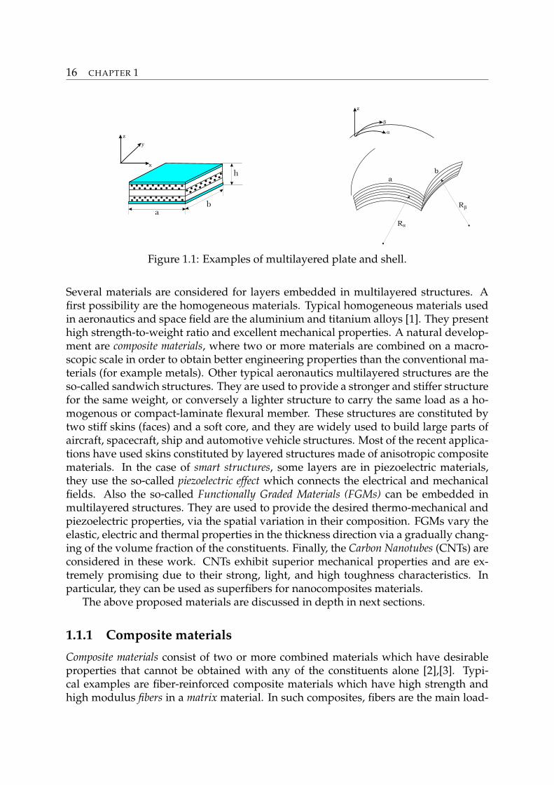
Advanced structures considered in this work are multilayered two-dimensional struc-tures embedding several layers with different properties: mechanical, thermal or elec-trical. As two-dimensional structures we consider those with a dimension, usually thethickness, negligible with respect to the other two in the in-plane directions. Typicaltwo-dimensional structures are plates and shells. Plates do not have any curvaturealong the two in-plane directions, they are flat panels. Shells are two-dimensionalstructures with curvature along the two in-plane directions. In the case of plates, a rec-tilinear Cartesian reference system is employed. In the case of shells, the introductionof a curvilinear reference system is necessary (see Fig. 1.1). In both plate and shellcases, the third axis in the thickness direction is always rectilinear.
15
16 CHAPTER 1
Figure 1.1: Examples of multilayered plate and shell.
Several materials are considered for layers embedded in multilayered structures. Afirst possibility are the homogeneous materials. Typical homogeneous materials usedin aeronautics and space field are the aluminium and titanium alloys [1]. They presenthigh strength-to-weight ratio and excellent mechanical properties. A natural develop-ment are composite materials, where two or more materials are combined on a macro-scopic scale in order to obtain better engineering properties than the conventional ma-terials (for example metals). Other typical aeronautics multilayered structures are theso-called sandwich structures. They are used to provide a stronger and stiffer structurefor the same weight, or conversely a lighter structure to carry the same load as a ho-mogenous or compact-laminate flexural member. These structures are constituted bytwo stiff skins (faces) and a soft core, and they are widely used to build large parts ofaircraft, spacecraft, ship and automotive vehicle structures. Most of the recent applica-tions have used skins constituted by layered structures made of anisotropic compositematerials. In the case of smart structures, some layers are in piezoelectric materials,they use the so-called piezoelectric effect which connects the electrical and mechanicalfields. Also the so-called Functionally Graded Materials (FGMs) can be embedded inmultilayered structures. They are used to provide the desired thermo-mechanical andpiezoelectric properties, via the spatial variation in their composition. FGMs vary theelastic, electric and thermal properties in the thickness direction via a gradually chang-ing of the volume fraction of the constituents. Finally, the Carbon Nanotubes (CNTs) areconsidered in these work. CNTs exhibit superior mechanical properties and are ex-tremely promising due to their strong, light, and high toughness characteristics. Inparticular, they can be used as superfibers for nanocomposites materials.
The above proposed materials are discussed in depth in next sections.
1.1.1 Composite materials
Composite materials consist of two or more combined materials which have desirableproperties that cannot be obtained with any of the constituents alone [2],[3]. Typi-cal examples are fiber-reinforced composite materials which have high strength andhigh modulus fibers in a matrix material. In such composites, fibers are the main load-
INTRODUCTION 17
carrying members and the matrix material keeps the fibers together, acts as a load-transfer medium between fibers, and protects them from being exposed to the envi-ronment. Fibers have a very high length-to-diameter ratio and their properties aremaximized in a given direction. Paradoxically, short fibers (whiskers) exhibit betterstructural properties than long fibers. The fibers and matrix materials usually em-ployed in composites can be metallic or non-metallic. The fiber materials can be com-mon metals like aluminum, copper, iron, nickel, steel, titanium, or organic materiallike glass, boron and graphite [2].
In the case of structural applications, for example in aeronautics field, fiber-reinforcedcomposite materials are often a thin layer called lamina. Typical structural elements,such as bars, beams, plates or shells are formed by stacking the layers to obtain desiredstrength and stiffness. Fiber orientation in each lamina and stacking sequence of thelayers can be chosen to achieve desired strength and stiffness for a specific application.
The main disadvantages of laminates made of fiber-reinforced composite materialsare the delamination and the fiber debonding. Delamination is caused by the mismatchof material properties between layers, which produces shear stresses between the lay-ers, especially at the edges of a laminate. Fiber debonding is caused by the mismatchof material properties between matrix and fiber. Also, during manufacturing of lami-nates, material defects such as interlaminar voids, delamination, incorrect orientation,damaged fibers and variation in thickness may be introduced [4].
In formulating the constitutive equations of a lamina we assume that: (a) a laminais a continuum: no gaps or empty spaces exist; (b) a lamina behaves as a linear elasticmaterial. The assumption (a) permits to consider the macromechanical behavior of alamina. The assumption (b) implies that the generalized Hooke’s law is valid.
Sandwich structures are a kind of composite structures that are widely used in theaerospace, aircraft, marine, and automotive industries because they are lightweightwith high bending stiffness. In general, the face sheets of sandwich panels consist ofmetals or laminated composites while the core is made of corrugated sheet, foam, orhoneycomb. The commonly used core materials include aluminum, alloys, titanium,stainless steel, and polymer composites. The core supports the skin, increases bendingand torsional stiffness, and carries most of the shear load [5],[6]. Structural sandwichesmost often have two faces, identical in material and thickness, which primarily resistthe in-plane and lateral (bending) loads. However, in special cases the faces may differin either thickness or material or both, because one face is the primary load-carryingand low-temperature portion, while the other face must withstand an elevated tem-perature, corrosive environment, etc.
1.1.2 Piezoelectric materials
The phenomena of piezoelectricity is a peculiarity of certain class of crystalline mate-rials. The piezoelectric effect is a linear energy conversion between mechanical andelectrical fields. The linear conversion between the two fields is in both directions,defining a direct or converse piezoelectric effect. The direct piezoelectric effect generates
18 CHAPTER 1
an electric polarization by applying mechanical stresses. On the contrary, the conversepiezoelectric effect induces mechanical stresses or strains by applying an electric field.These two effects represent the coupling between the mechanical and electrical field,that is mathematically expressed by means of piezoelectric coefficients. First applica-tions for piezoelectric materials were sound, ultrasound sensors and sources. These arestill actual, but, in recent years, piezoelectricity has found renewed interest, as activeintelligent structures with self-monitoring and self-adaptive capabilities [7]-[9]. Typi-cal applications of piezoelectric materials in aerospace field are listed below.
Vibration damping. Nearly every structure in aerospace engineering is subjected tovibrations. In some cases such dynamic loads can be more dangerous than theapplied static loads. By implementing sensors and actuators in such structures,the dynamic vibrations can be measured and then actively damped. Typical ex-amples are vibration problems for the rotor wings in helicopters, sound dampingin the cockpit or cabin of civil planes.
Shape adaption of aerodynamics surfaces. In modern airplane the aerodynamic sur-faces can be optimized only for a certain airspeed and flight altitude. Wings thatare able to change their geometry according to the actual demands could lead toan increase in efficiency.
Active aeroelastic control. Typical problems of aeroelasticity like flutter or buffetingcan be reduced by the use of adaptive materials.
Shape control of optical and electromagnetic devices. Structures in aerospace field aresubjected to rapid and high temperature variations due to changing exposure tothe sunlight. Optical surfaces like mirrors and lenses, electromagnetic antennasand reflectors are highly sensitive to thermal deformations. A remedy to theseproblems could be the use of adaptive materials.
Health monitoring. In aerospace structures microscopic cracks are tolerable up to acertain limit. Smart structures could monitor these stresses and then apply anadditional control mechanism to maintain the safety.
1.1.3 Functionally graded materials
The severe temperature loads involved in many engineering applications, such as ther-mal barrier coatings, engine components or rocket nozzles, require high temperatureresistant materials. In Japan in the late 1980s the concept of Functionally Graded Ma-terials (FGMs) has been proposed as a thermal barrier material. FGMs are advancedcomposite materials wherein the composition of each material constituent varies grad-ually with respect to spatial coordinates [10]. Therefore, in FGMs the macroscopicmaterial properties vary continuously, distinguishing them from laminated compos-ite materials in which the abrupt change of material properties across layer interfacesleads to large interlaminar stresses allowing for damage development [11].
INTRODUCTION 19
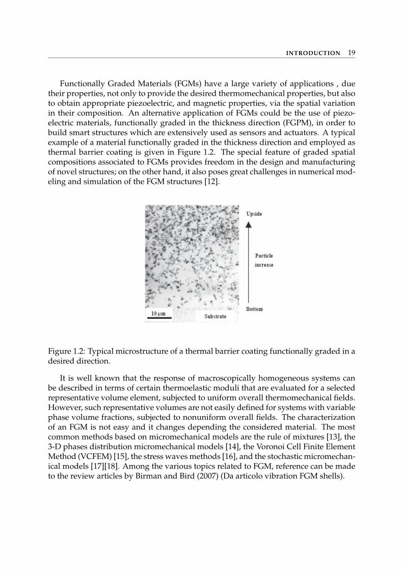
Functionally Graded Materials (FGMs) have a large variety of applications , duetheir properties, not only to provide the desired thermomechanical properties, but alsoto obtain appropriate piezoelectric, and magnetic properties, via the spatial variationin their composition. An alternative application of FGMs could be the use of piezo-electric materials, functionally graded in the thickness direction (FGPM), in order tobuild smart structures which are extensively used as sensors and actuators. A typicalexample of a material functionally graded in the thickness direction and employed asthermal barrier coating is given in Figure 1.2. The special feature of graded spatialcompositions associated to FGMs provides freedom in the design and manufacturingof novel structures; on the other hand, it also poses great challenges in numerical mod-eling and simulation of the FGM structures [12].
Figure 1.2: Typical microstructure of a thermal barrier coating functionally graded in adesired direction.
It is well known that the response of macroscopically homogeneous systems canbe described in terms of certain thermoelastic moduli that are evaluated for a selectedrepresentative volume element, subjected to uniform overall thermomechanical fields.However, such representative volumes are not easily defined for systems with variablephase volume fractions, subjected to nonuniform overall fields. The characterizationof an FGM is not easy and it changes depending the considered material. The mostcommon methods based on micromechanical models are the rule of mixtures [13], the3-D phases distribution micromechanical models [14], the Voronoi Cell Finite ElementMethod (VCFEM) [15], the stress waves methods [16], and the stochastic micromechan-ical models [17][18]. Among the various topics related to FGM, reference can be madeto the review articles by Birman and Bird (2007) (Da articolo vibration FGM shells).
20 CHAPTER 1
1.1.4 Carbon nanotubes
Carbon nanotubes (CNT) have exceptional mechanical properties (Young’s modulus,tensile strength, toughness, etc), which are due to their molecular structure consistingof single or multiple sheets of graphite wrapped into seamless hollow cylinders [19].Due to the large stiffness, strength and high aspect ratio of CNTs, it is expected thatby evenly dispersing them throughout a polymer matrix one can produce compos-ites with considerably improved overall effective mechanical properties. Furthermore,CNTs have a relatively low density of about 1.75 g/cm−3 and, therefore, nanotube re-inforced polymers (NRPs) excel due to their extremely high specific stiffness, strengthand toughness. This has already been demonstrated in experiments, both for thermo-plastic [20] and thermosetting [21] polymer matrices.
The study of the vibration and frequency analysis of embedded CNTs is a majortopic of current interest. Since controlled experiments to measure the properties of in-dividual CNT at the nanoscale are extremely difficult, computational simulations havebeen regarded as a powerful tool. However, computational simulations for predictingproperties of CNTS fall into two major categories: molecular dynamics (MD) and con-tinuum mechanics. Although MD simulation has been successfully used for simulat-ing the properties of the material with microstructures, this method is time consumingand formidable especially for large-scale complex systems. Recently, solid mechanicswith continuum elastic models, such as beam and shell models, have been widely andsuccessfully used to study mechanical behavior of CNTs [22],[23]. Moreover, interestin double-walled nanotubes (DWNTs) is rising due to the progress in large-scale syn-thesis of DWNTs. In these cases, it is anticipated that intertube radial displacementsof Multiwalled carbon nanotubes (MWNTs), defined by substantially non-coincidentaxes of the nested nanotubes, would come to play a significant role and it must beaccounted in the considered continuum model [24].
1.2 Theoretical models for thin-walled composites struc-tures
In recent years, considerable attention has been paid to the development of appropriatetwo-dimensional shell theories that can accurately describe the response of multilay-ered anisotropic thick shells. In fact, thick shell component analysis and fatigue designrequire an accurate description of local stress fields to include highly accurate assess-ment of localized regions where damage is likely to take place. As mentioned in theprevious section, examples of multilayered shell structures used in modern aerospacevehicles are laminated constructions made of anisotropic composite materials, sand-wich panels, layered structures used as thermal protection, or intelligent structuralsystem embedding piezolayers.
It was pointed out by Koiter [25] that, for traditional isotropic one-layer shells, re-finements of Love’s first approximation theory are meaningless unless the effects oftransverse shear and normal stress are both taken into account in a refined theory.
INTRODUCTION 21
Layered shells deserve special attention. These are characterized by a noncontinu-ous material properties distribution in the thickness direction and further requisitesbecome essential for a reliable modelling of such structures. Among these, the fulfill-ment of both continuity of displacement and transverse shear and normal stresses atthe interface between two adjacent layers is such a necessary desideratum. In Ref. [26]these requisites are referred to as C0
z requirements that state that both displacementsand transverse stress components are C0-continuous functions in the thickness shellcoordinate z. An increasing role is played by the C0
z requirements and by Koiter’s rec-ommendation in the case of laminated shells made of composite materials presentlyused in aerospace structures. These materials exhibit higher values of Young’s moduliorthotropic ratio (EL/ET = EL/Ez = 5 ÷ 40; L denotes the fiber directions,whereas Tand z are two-direction orthogonal to L) and the lower transverse shear moduli ratio(GLT /EL ≈ GTT /EL = 1
10÷ 1
200) leading to higher transverse shear and normal stress
deformability in comparison to isotropic cases. Approximated three-dimensional solu-tions by Noor and Rarig [27] and Noor and Peters [28],[29] and more recent exact three-dimensional solutions by Ren [30] and Varadan and Bhaskar [31] have numericallyconfirmed the need of the previously mentioned refinements for static and dynamiccylindrical shell problems. In particular, the fundamental role played by transversenormal stress σzz was underlined. Nevertheless, three-dimensional elasticity solutionsare only available in a very few cases and these are mainly related to simple geometries,a specific stacking sequence of the lamina, and linear problems. In the most generalcases and to minimize the computational effort, two-dimensional models are preferredin practice.
Starting from the early work by Shtayerman [32] many two-dimensional modelshave been proposed for anisotropic layered shells. The so-called axiomatic approach[33] (where a certain displacement or stress field is postulated in the shell thicknessdirection) and asymptotic methods [34]-[40] (where the three-dimensional equationsare expanded in terms of an introduced shell parameter) have both been applied to de-rive simplified analysis. Exhaustive overviews on these topics can be found in manypublished review papers. Classical theories were reviewed by Bert [41]. An interest-ing overview, including works that appeared in Russian literature, can be found inthe book by Librescu [42]. Recent developments in the Russian school concerning thefulfillment of the C0
z requirements were overviewed by Grigolyuk and Kulikov [43].Reviews on finite element shell formulations can be found in the work by Dennis andPalazotto [44], Merk [45], and Di and Ramm [46]. Recent articles on the application ofasymptotic methods to anisotropic shells can be found in Fettahlioglu and Steele [47],Widera and Logan [48], Widera and Fan [49] and Spencer et al. [50]. Two exhaustiveand more recent surveys have been provided by Kapania [51] and Noor and Burton[183] that address a complete overview of different aspects of multilayered shells mod-elings. Herein, attention is focused on the axiomatic approach. A short review of thisapproach follows.
Classical displacement formulations start by assuming a linear or higher-order ex-pansion for the displacement fields in the thickness direction. In-plane and transversestresses are then computed by means of Hooke’s law. According to this procedure, it is
22 CHAPTER 1
found that transverse stresses (both shear and normal components) are discontinuousat the interfaces. To overcome these difficulties, these stresses are evaluated a poste-riori in most applications by implementing a post-processing procedure, e.g., throughthe thickness integration of the three-dimensional indefinite equation of equilibrium.A few examples in which a layer-wise model (LWM) description is used (the num-ber of the unknowns depends on the number of layers) are works by Hsu and Wang[53], Cheung and Wu [54], and Barbero et al. [55]. Others, in which an equivalentsingle-layer model (ESLM) description was preferred, are the works by Hildebrand etal. [56], Whitney and Sun [57], Reddy and Liu [234], Librescu et al. [59], and Dennisand Palazotto [44],[60]. The interesting theory by Rath and Das [61] should be men-tioned from the ESLM analysis, where interlaminar transverse shear continuity was apriori fulfilled in both the symmetrical and unsymmetrical case through the thicknessresponse of layered shells. A particular example of the theory in Ref. [61] was analyzedin Ref. [62] for symmetrically laminated cylinders. The numerical analysis reported inthe cited works conclude the following:
1. An a priori description of transverse stress cannot account for LWMs based onthe displacement formulation.
2. Layer-wise (LW) analysis usually lead to a better description than ESLM ones;such a superiority is more evident for arbitrarily laminated shells with increasinglayers.
3. The ESLM analysis experienced difficulties in accurately describing a σzz and therelated consequences.
4. The mentioned post-processing procedure for the calculation of transverse stressescannot be implemented for most of the available models in the general case ofasymmetric in-plane displacement fields (i.e., two different results could be ob-tained for the stress distributions by starting from the top or from the bottomshell surface).
Reissner [63],[64] proposed a mixed variational equation for the purpose of over-coming the impossibility of fulfilling a priori the interlaminar continuity for both trans-verse shear and normal stresses, which furnishes equilibrium and constitutive equa-tions that are consistent with an assumed displacement and transverse stress field.Similar discussion and conclusions can be read in the overview paper by Grigolyukand Kulikov [43]. This tool was applied to shells by Bhaskar and Varadan [65] andJing and Tzeng [66] for the case of ESLM analysis. Both works neglected the transversenormal stress. Related results confirmed that the use of Reissner’s mixed variationalequations associated to an ESLM description is not sufficient to describe accurately theσzz effects. Therefore, the use of Reissner equation requires a layer-wise description.The convenience of referring to a Reissner mixed variational equation was shown in[26],[67]-[73]. In particular, it was shown that the proposed layer-mixed descriptiongives an excellent a priori description of the transverse shear and normal stress fields.
INTRODUCTION 23
It is a well-established result obtained from traditional isotropic shell structuresanalysis [74]-[77] that accurate two-dimensional shell modelling cannot come with-out an equivalently accurate description of the curvature terms. The neglectfulness ofterms of type h = R (thickness to radii shell ratio) or the use of Donnell’s shallow-shelltype approximations could be very restrictive in thick-shell analysis. In fact, as shownby Soldatos [78], Carrera [79], and Jing and Tzeng [66] any refinement related to thefulfillment of C0
z requirements would be meaningless unless curvature terms are welldescribed. For this reason, no assumption will be introduced in this work concerningcurvature terms.
1.2.1 Modelling of piezoelectric structures
In most applications, the piezoelectric layers are embedded in multilayer structuresmade of anisotropic composite materials. The efficient use of piezoelectric materials inmultilayer structures requires accurate evaluation of mechanical and electric variablesin each layer. Classical shell models such as classical lamination theory (CLT) and first-order shear deformation theory (FSDT) can lead to large discrepancies with respect tothe exact solution. Improvements can be introduced by using equivalent single-layermodels with higher-order kinematics. However, much better results can be obtainedthrough the use of layerwise models. For recent indications of the superiority of LWMsover ESLMs, see [80].
The advantages of the Reissner Mixed Variational Theorem (RMVT) with respect toother approaches that mostly make use of the Principle of Virtual Displacement (PVD)were shown in [81],[82]. The Unified Formulation (UF) was used there to create anhierarchical shell formulation with variable kinematics (relative to displacements andtransverse stresses) in each layer. Attention was restricted to pure mechanical prob-lems. UF has been extended to closed-form and finite-element solutions of a piezoelec-tric plate in [83] and [84], respectively; PVD was used and only the displacements andthe electrical potential were considered as unknown variables. The main advantage ofRMVT is the possibility of fulfilling a priori the continuity conditions for the transverseelectromechanical variables (electric displacement and stresses). Indeed, the disconti-nuity of electromechanical properties at the layer interface requires a discontinuousfirst derivative of the same variables.
Attempts to introduce the C0z -requirements in piezoelectric continua have been
made in [85],[86]. Closed form and FEs solutions were considered in these last pa-pers, respectively. Attention was restricted to the fulfillment of C0
z -requirements fortransverse shear and normal stress components. Such an extension is herein stated asa "partial" RMVT application. The complete fulfillment of the C0
z -requirements to bothelectrical and mechanical variables has been provided in the companion paper [87],devoted to FE analysis and plate geometries. Such a contribution has been called a"full" extension of RMVT to piezoelectric continua.
A few papers on piezoelectric shells exist in the literature, in particular for the FEmethod. Layerwise methods were considered in [220]. FE piezoelectric shells havebeen considered in [89]. Cho and Roh [90] proposed geometrically exact shell elements,
24 CHAPTER 1
while Kogl and Bucalem [91] gave the extension of MITC4 type element to piezoelectricshell structures. Review and assessment have been given in [92]. Three dimensionalpiezoelasticity solutions have been addressed in [93]-[96]. Wang et al. [93] and Shakeriet al. [94] dealt with vibration problems. Chen et al. [95] addressed cylindrical shellwith very thin piezoelectric layers. Only a piezoelectric layer was instead considered in[96]. No results are available in which both mechanical and piezoelectric layers (withthickness comparable to the mechanical layers) are analyzed.
The full version of RMVT has been extended to piezoelectric shells in [97] and [98].These are the natural extension of the previous works [72],[73],[219],[100] that dealwith the plates.
1.2.2 Modelling of FGM structures
The concept of Functionally Graded Material was first proposed as thermal barrier ma-terial. Therefore, the thermo-mechanical problem in FGMs is a major topic of currentinterest.
Over the last decade, extensive research has been carried out on the modeling ofshells comprising FGM layers. Pelletier and Vel, in [101], have provided an exact so-lution for the steady-state thermoelastic response of functionally graded orthotropiccylindrical shells. The equilibrium equations are solved by the power series methodand the temperature field are obtained by solving the heat conduction equations. Thecylindrical shells are analyzed using the Flugge and the Donnell theories. In [102]Shao has derived a series solution for a functionally graded circular hollow cylinder,using a multi-layered approach based on the laminated composite theory. The mate-rial properties are assumed to be temperature-independent and radial dependent, butare assumed to be homogenous in each layer. The temperature profile along the thick-ness is calculated by means of the heat conduction equations. A functionally gradedcircular hollow cylinder has also been analyzed by Liew et al. in [103]. In this case,the solutions are obtained through a novel limiting process that employs the solutionsof homogeneous hollow circular cylinders. The temperature distribution is assumedin the radial direction. Vel and Baskiyar [104] have presented an analytical solutionfor a functionally graded tube with arbitrary variation of the material properties in theradial direction and subjected to steady thermomechanical loads. The heat conduc-tion and thermoelasticity equations are solved using the power series method. In [105]Abrinia et al. have proposed an analytical method to compute the radial and circumfer-ential stresses in a thick FGM cylindrical vessel under the influence of internal pressureand temperature. In this paper it is assumed that the modulus of elasticity and thermalcoefficient of expansion vary through the thickness of the FGM material, according toa power law relationship. Shao and Wang [106] have performed a three-dimensionalthermo-elastic analysis of a functionally graded cylindrical panel with finite length andsubjected to non uniform mechanical and steady-state thermal loads. The thermal andmechanical properties are assumed to be temperature independent and continuouslyvary in the radial direction of the panel.
INTRODUCTION 25
1.2.3 Modelling of CNTs
Two basic methods are used to simulate the mechanical behavior of nanostructures:atomistic-based modelling approaches and continuum approaches. In the former, thevibrational behavior of CNTs is investigated using an atomistic finite element modelwith beam elements and concentrated masses [107],[108]. But, the computational ef-fort necessary for these methods does not permit simulations of real size multi-walledCNTs. For these reasons, continuum approaches are preferred to atomistic-based ones.
In literature, many researchers have used beam models to analyze the mechani-cal behavior of carbon nanotubes. Among these, Wang [109] and Aydogdu [110],[221]have studied the vibration problem in multi-walled carbon nanotubes (MWCNTs) viathe Timoshenko beam model and the generalized shear deformation theory, respec-tively. In [112], Amin et al. have presented a double elastic beam model for frequencyanalysis in a double-walled carbon nanotube (DWNT) embedded in an elastic ma-trix. The analysis has been based on both Euler-Bernoulli and Timoshenko beam the-ories, considering intertube radial displacements. Chang and Lee have also employedthe Timoshenko beam model, in [113], to study the vibration frequency of a fluid-conveying SWCNT. An assessment of the Timoshenko beam models has been accom-plished by Zhang et al. in [114] in determining the vibration frequencies of SWCNTs.
However, it is also possible to analyze carbon nanotubes using shell models. In[115], Dong et al. have presented an analytical method to investigate wave propaga-tion in MWNTs, using a laminated cylindrical shell model. Each of the concentric tubesof the MWNT was an individual elastic shell and is coupled to adjacent tubes throughthe van der Waals interaction. Foo has adopted the Donnell thin shell theory for thevibration analysis of SWCNTs [116]. Wang and Zhang [117] have also proposed a two-dimensional elastic shell model to characterize the deformation of single-walled car-bon nanotubes and they have concluded that this model can be established with well-defined effective thickness. He et al. have developed an elastic multiple shell modelfor the vibration and buckling analysis of MWCNTs [118],[119], which accounts for thedependence of vdW interaction coefficients on the change of interlayer spacing andthe radii of the tubes. Finally, in [120] a continuum elastic double-shell model, basedon von Kàrmàn-Donnell-type non-linear differential equations, has been employed tostudy the buckling and post-buckling behavior of DWNTs subjected to torsional load.Each DWNT tube has been described as an individual elastic shell, which is subject tothe van der Waals interaction between the inner and outer nanotubes.

Chapter 2
Refined and advanced shell models
Different refined and advanced shell/plate models are contained in the Carrera’s Unified Formu-lation (CUF). The CUF permits to obtain, in a general and unified manner, several models thatcan differ by the chosen order of expansion in the thickness direction, by the equivalent singlelayer or layer wise approach and by the variational statement used. These models are here de-fined directly for the shells, according to different geometrical assumptions: plates are particularcases when the shell has infinite curvature radius. By considering the appropriate constitutiveequations, the CUF can be applied to the analysis of the advanced materials described in theprevious section. The refined theories are higher order theories based on the principle of virtualdisplacements and they can be extended to multifield problems by considering the modelling oftemperature and electric potential. Advanced theories are theories based upon the Reissner’smixed variational theorem in which secondary variables, such as the transverse shear/normalstresses and the transverse normal electric displacement, are "a priori" modelled. A completesystem of acronyms is introduced to characterize these two-dimensional theories.
2.1 Unified Formulation
The main feature of the Unified Formulation by Carrera [26] (CUF) is the unified man-ner in which the field variables are handled. If one considers a displacements formu-lation, the displacement field is written by means of approximating functions in thethickness direction as follows:
δuk(ξ1, ξ2, ξ3) = Fτ (ξ3)δuk
τ (ξ1, ξ2) , uk(ξ1, ξ2, ξ3) = Fs(ξ
3)uks(ξ
1, ξ2) , τ, s = 0, 1, ..., N ,(2.1)
where (ξ1, ξ2, ξ3) is a curvilinear reference system, defined in the next section, and thedisplacement u = u, v, w is referred to such system. δ indicates the virtual variationand k identifies the layer. Fτ and Fs are the so-called thickness functions dependingonly on ξ3. us are the unknown variables depending on the coordinates ξ1 and ξ2.τ and s are sum indexes and N is the order of expansion in the thickness directionassumed for the displacements.
In the case of Equivalent Single Layer (ESL) models, a Taylor expansion is em-
27
28 CHAPTER 2
ployed as thickness functions:
u = F0 u0 + F1 u1 + . . . + FN uN = Fs us , s = 0, 1, . . . , N , (2.2)
F0 = (ξ3)0 = 1, F1 = (ξ3)1 = ξ3, . . . , FN = (ξ3)N . (2.3)
Classical theories, such as the First-order Shear Deformation Theory (FSDT), can be ob-tained from an ESL model with N = 1, by imposing a constant transverse displacementthrough the thickness via penalty techniques. The Classical Lamination Theory (CLT)can be also obtained from FSDT via an opportune penalty technique which imposesan infinite shear correction factor. It is important to remember that the ESL theorieswhich have transverse displacement constant and transverse normal strain εzz equalto zero and the first order ESL theory, show Poisson’s locking phenomena; this can beovercome via plane stress conditions in constitutive equations [121],[122].
In the case of Layer-Wise (LW) models, the displacement is defined at k-layer level:
uk = Ft ukt + Fb uk
b + Fr ukr = Fs uk
s , s = t, b, r , r = 2, ..., N , (2.4)
Ft =P0 + P1
2, Fb =
P0 − P1
2, Fr = Pr − Pr−2. (2.5)
in which Pj = Pj(ζk) is the Legendre polynomial of j-order defined in the ζk-domain:−1 < ζk < 1. The top (t) and bottom (b) values of the displacements are used asunknown variables and one can impose the following compatibility conditions:
ukt = uk+1
b , k = 1, Nl − 1. (2.6)
The LW models, in respect to the ESLs, allow the zig-zag form of the displacementdistribution in layered structures to be modelled. It is possible to reproduce the zig-zag effects also in the framework of the ESL description by employing the Murakamitheory. According to reference [123], a zig-zag term can be introduced into equation(2.7) as follows:
uk = F0 uk0 + . . . + FN uk
N + (−1)kζkukZ . (2.7)
Subscript Z refers to the introduced term. Such theories are called zig-zag (ZZ) theo-ries.
2.2 Geometrical relations
We define a thin shell as a three-dimensional body bounded by two closely spacedcurved surfaces, the distance between the two surfaces must be small in comparisonwith the other dimensions. The middle surface of the shell is the locus of points whichlie midway between these surfaces. The distance between the surfaces measured alongthe normal to the middle surface is the thickness of the shell at that point [124]. Shellsmay be seen as generalizations of a flat plate [125]; conversely, a flat plate is a special
REFINED AND ADVANCED SHELL MODELS 29
case of a shell having no curvature. In this section the fundamental equations of thinshell theory are presented in order to obtain the geometrical relations also for multifieldproblems. Geometrical relations for plates are seen as particular case of those for shells.The material is assumed to be linearly elastic and homogeneous, displacements areassumed to be small, thereby yielding linear equations; shear deformation and rotaryinertia effects are neglected, and the thickness is taken to be small.
2.2.1 Strain-displacement relations
The shell can be considered as a solid medium geometrically defined by a midsurface,given by the coordinates ξ1, ξ2, immersed in the physical space and a parameter repre-senting the thickness ξ3 of the medium around this surface. The geometrical relationsfor shells are derived by considering the linear part of the 3D Green-Lagrange straintensor [126], that is expressed in the following formula:
ε′ij = (giu,j + gju,i) , i, j = 1, 2, 3 , (2.8)
where comma indicates the partial derivative of the displacements in respect to thecurvilinear coordinates (ξ1, ξ2, ξ3) and gi are the 3D base vectors of the curvilinear ref-erence system.In order to calculate the derivatives of the displacements and the 3D base vectors, oneneeds to define the 3D chart Φ, that allows to express the cartesian coordinates (x, y, z)in function of the curvilinear coordinates:
Φ(ξ1, ξ2, ξ3) = φ(ξ1, ξ2) + ξ3a3(ξ1, ξ2) . (2.9)
It is defined by means of the 2D chart φ and the unit vector a3, that will be introducedbelow (see Fig.2.1). Starting from Φ, one can calculate the 3D covariant basis (g1, g2, g3)as follows:
gm =∂Φ(ξ1, ξ2, ξ3)
∂ξmm = 1, 2, 3 , (2.10)
that is a local basis and it is defined in each point of the shell volume. The 3D con-travariant basis (g1, g2, g3) can be inferred from the 3D covariant basis by the relations:
gm · gn = δnm m,n = 1, 2, 3 , . (2.11)
where δ denotes the Kronecker symbol (δnm = 1 if m = n and 0 otherwise).
The vectors aα and a3, that form the covariant basis of the plane tangent to the mid-surface at each point, are calculated from the 2D chart as follows:
30 CHAPTER 2
y
x
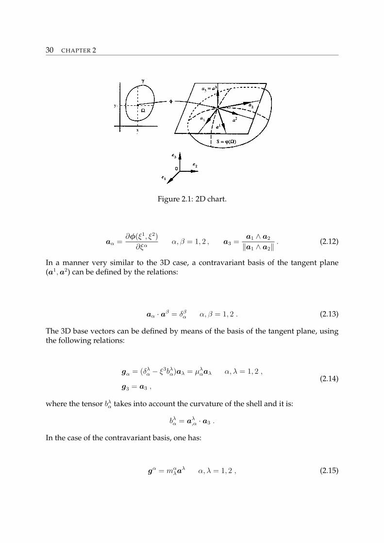
Figure 2.1: 2D chart.
aα =∂φ(ξ1, ξ2)
∂ξαα, β = 1, 2 , a3 =
a1 ∧ a2
‖a1 ∧ a2‖ . (2.12)
In a manner very similar to the 3D case, a contravariant basis of the tangent plane(a1,a2) can be defined by the relations:
aα · aβ = δβα α, β = 1, 2 . (2.13)
The 3D base vectors can be defined by means of the basis of the tangent plane, usingthe following relations:
gα = (δλα − ξ3bλ
α)aλ = µλαaλ α, λ = 1, 2 ,
g3 = a3 ,(2.14)
where the tensor bλα takes into account the curvature of the shell and it is:
bλα = aλ
,α · a3 .
In the case of the contravariant basis, one has:
gα = mαλaλ α, λ = 1, 2 , (2.15)
REFINED AND ADVANCED SHELL MODELS 31
where mαλ is the inverse of the tensor µλ
α introduced in the previous relations (2.14):
mαλ = (µ−1)α
λ .
The derivatives of the displacements are calculated in the following way:
∂u
∂ξα= Fτ
∂uτ
∂ξα, α = 1, 2, 3 , (2.16)
where:
∂uτ
∂ξα=
∂
∂ξα(uτλ
aλ + uτ3a3) , λ = 1, 2 , (2.17)
and, for convenience reasons, it is here assumed that (u, v, w) = (u1, u2, u3). Then, onehas:
∂
∂ξα(uτλ
aλ) = uτλ|αaλ + bλαuτλ
a3 , α, λ = 1, 2 , (2.18)
where | indicates the covariant derivative, that is defined as follows:
uτλ|α = uτλ,α− Γγ
λαuγ , γ = 1, 2 . (2.19)
The Γγλα is the surface Christoffel symbol and it reads:
Γγλα = aλ,α · aγ .
For more details about the mathematical definitions, one can refer to the book of Chapelleand Bathe [126].
Cylindrical geometry
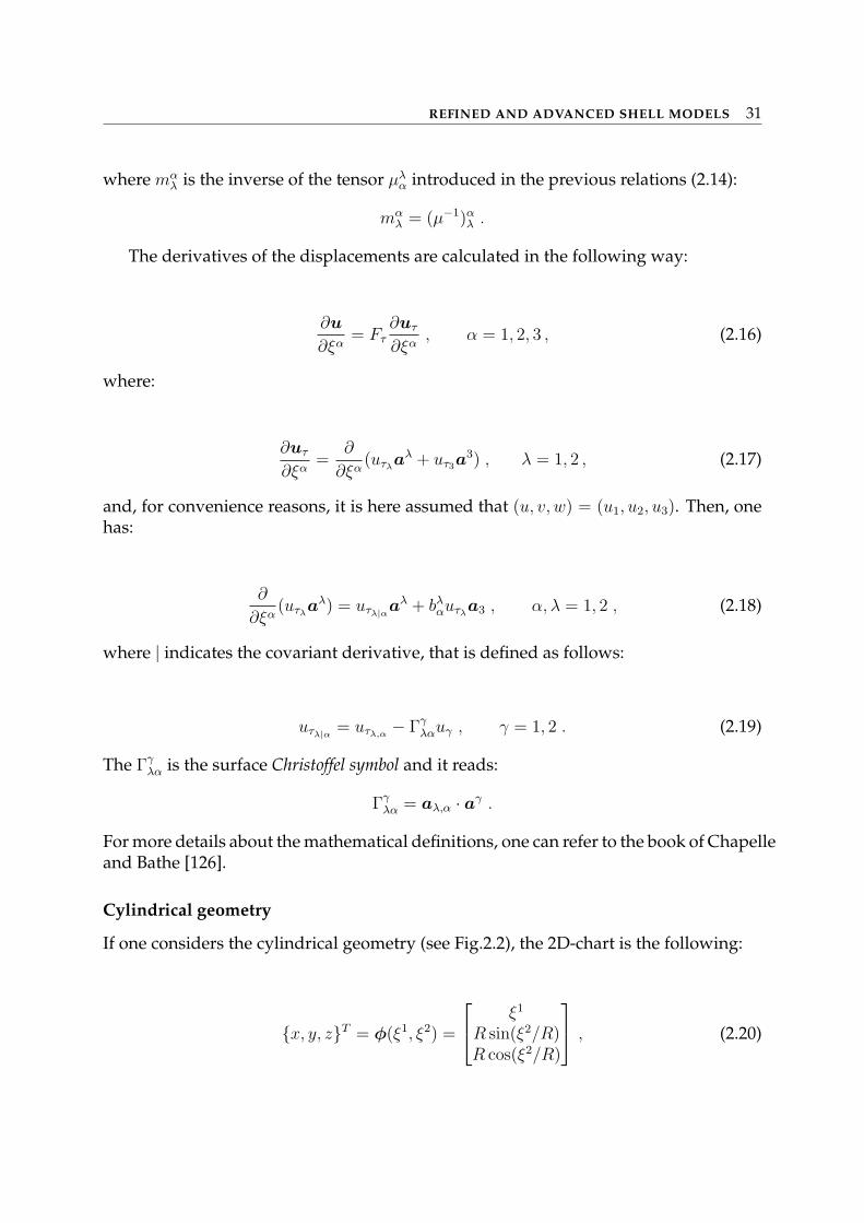
If one considers the cylindrical geometry (see Fig.2.2), the 2D-chart is the following:
x, y, zT = φ(ξ1, ξ2) =
ξ1
R sin(ξ2/R)R cos(ξ2/R)
, (2.20)
32 CHAPTER 2
ξ1
ξ2
ξ3
x
y
z
R
L
Figure 2.2: Cylindrical geometry.
where R is the curvature radius of the cylinder, as indicated in the Figure 1.1. Us-ing the 2D chart, one can calculate the 3D base vectors (2.14) and the derivatives ofthe displacements (2.16), following the procedure explained in the previous section.Substituting in the 3D Green-Lagrange strain tensor (2.8), one obtains the followingstrain-displacement relations, valid for the cylinder:
ε′11 = Fτuτ,1 ,
ε′22 = Fτ
[(1 +
ξ3
R
)wτ
R+
(1 +
ξ3
R
)vτ,2
],
ε′12 = Fτ
[uτ,2 +
(1 +
ξ3
R
)vτ,1
]= ε21 ,
ε′13 = wτ,1Fτ + uτFτ,3 ,
ε′23 = Fτ
[wτ,2 − vτ
R
]+ Fτ,3
[(1 +
ξ3
R
)vτ
],
ε′33 = wτFτ,3 .
(2.21)
The geometrical relations in matrix form are:
εp =(Dp + Ap)u ,
εn =(Dnp + Dnz −An)u ,(2.22)
where (p) indicates the in-plane strain components (ε′11, ε′22, ε
′12) and (n) the transverse
components (ε′13, ε′23, ε
′33). The differential operators used above are defined as follows:
Dp =
∂1 0 00 H∂2 0∂2 H∂1 0
, Dnp =
0 0 ∂1
0 0 ∂2
0 0 0
, Dnz = ∂3 ·Anz = ∂3 ·
1 0 00 H 00 0 1
, (2.23)
REFINED AND ADVANCED SHELL MODELS 33
Ap =
0 0 00 0 1
RH
0 0 0
,An =
0 0 00 1
R0
0 0 0
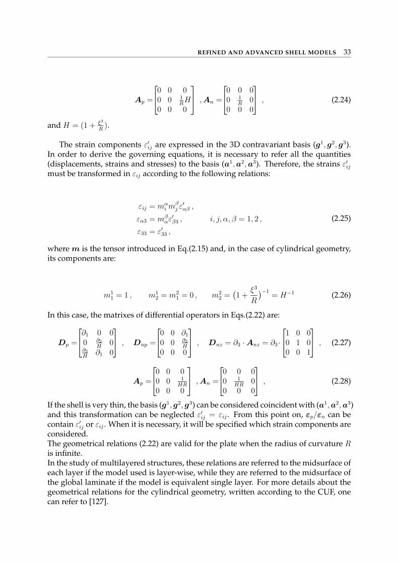
, (2.24)
and H = (1 + ξ3
R).
The strain components ε′ij are expressed in the 3D contravariant basis (g1, g2, g3).In order to derive the governing equations, it is necessary to refer all the quantities(displacements, strains and stresses) to the basis (a1,a2,a3). Therefore, the strains ε′ijmust be transformed in εij according to the following relations:
εij = mαi mβ
j ε′αβ ,
εα3 = mβαε′β3 , i, j, α, β = 1, 2 ,
ε33 = ε′33 ,
(2.25)
where m is the tensor introduced in Eq.(2.15) and, in the case of cylindrical geometry,its components are:
m11 = 1 , m1
2 = m21 = 0 , m2
2 =(1 +
ξ3
R
)−1= H−1 (2.26)
In this case, the matrixes of differential operators in Eqs.(2.22) are:
Dp =
∂1 0 00 ∂2
H0
∂2
H∂1 0
, Dnp =
0 0 ∂1
0 0 ∂2
H
0 0 0
, Dnz = ∂3 ·Anz = ∂3 ·
1 0 00 1 00 0 1
, (2.27)
Ap =
0 0 00 0 1
HR
0 0 0
,An =
0 0 00 1
HR0
0 0 0
, (2.28)
If the shell is very thin, the basis (g1, g2, g3) can be considered coincident with (a1, a2,a3)and this transformation can be neglected ε′ij = εij . From this point on, εp/εn can becontain ε′ij or εij . When it is necessary, it will be specified which strain components areconsidered.The geometrical relations (2.22) are valid for the plate when the radius of curvature Ris infinite.In the study of multilayered structures, these relations are referred to the midsurface ofeach layer if the model used is layer-wise, while they are referred to the midsurface ofthe global laminate if the model is equivalent single layer. For more details about thegeometrical relations for the cylindrical geometry, written according to the CUF, onecan refer to [127].
34 CHAPTER 2
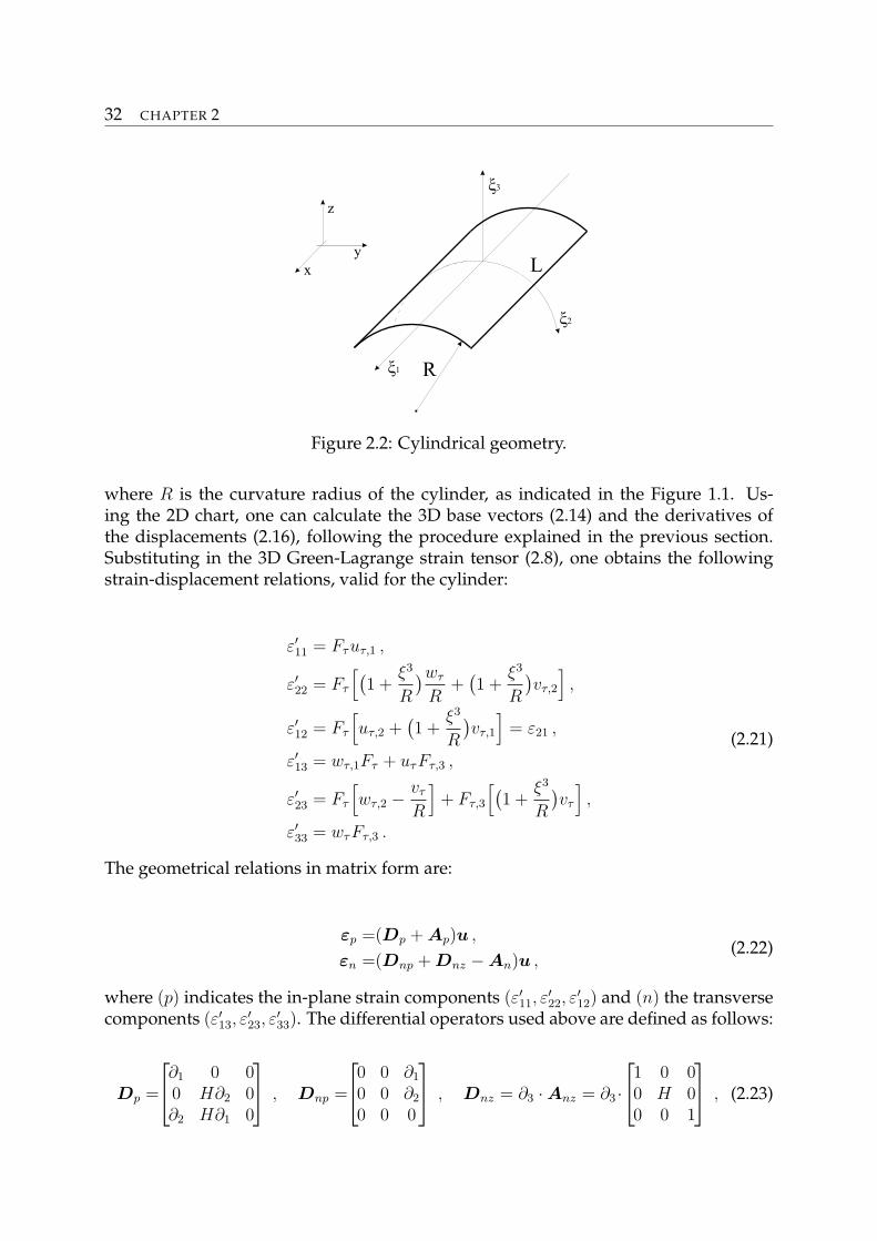
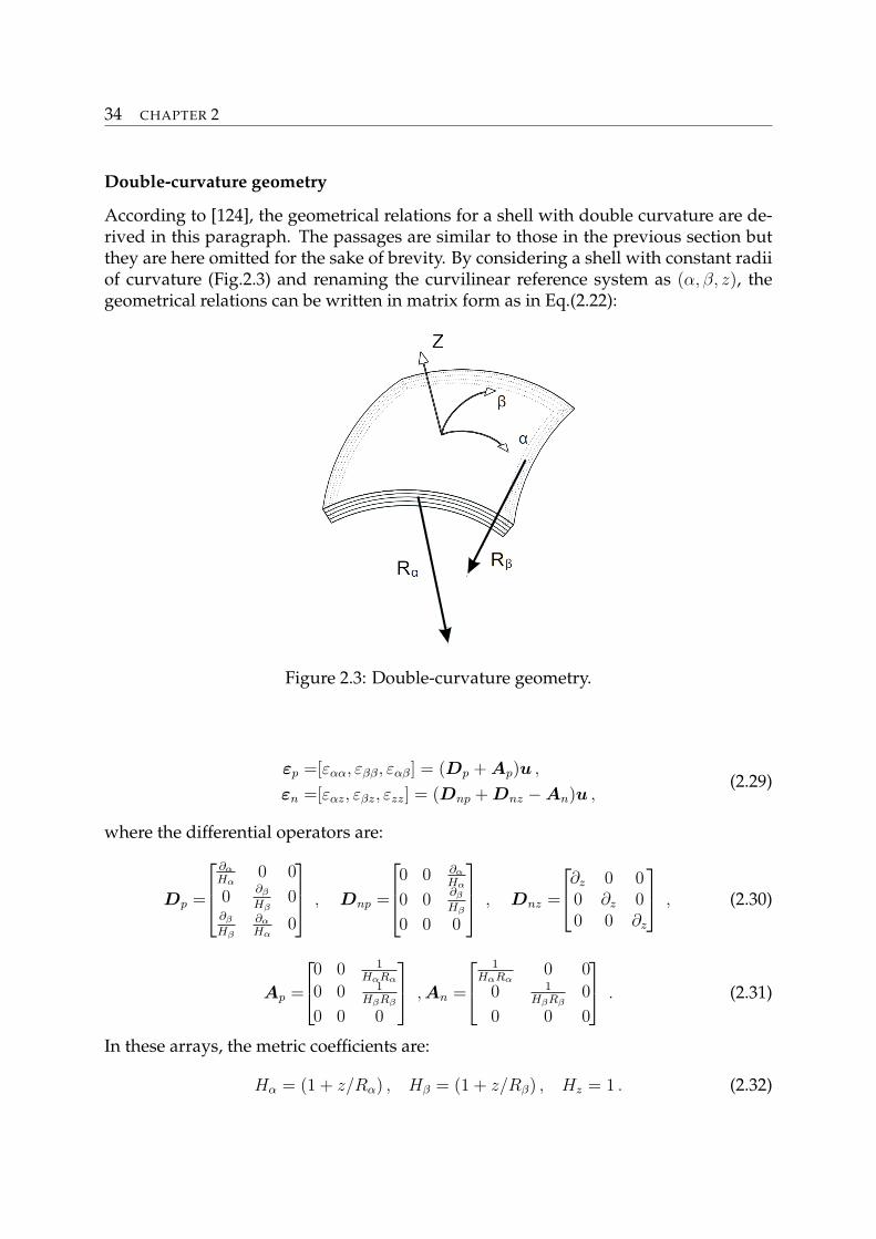
Double-curvature geometry
According to [124], the geometrical relations for a shell with double curvature are de-rived in this paragraph. The passages are similar to those in the previous section butthey are here omitted for the sake of brevity. By considering a shell with constant radiiof curvature (Fig.2.3) and renaming the curvilinear reference system as (α, β, z), thegeometrical relations can be written in matrix form as in Eq.(2.22):
Figure 2.3: Double-curvature geometry.
εp =[εαα, εββ, εαβ] = (Dp + Ap)u ,
εn =[εαz, εβz, εzz] = (Dnp + Dnz −An)u ,(2.29)
where the differential operators are:
Dp =
∂α
Hα0 0
0∂β
Hβ0
∂β
Hβ
∂α
Hα0
, Dnp =
0 0 ∂α
Hα
0 0∂β
Hβ
0 0 0
, Dnz =
∂z 0 00 ∂z 00 0 ∂z
, (2.30)
Ap =
0 0 1
HαRα
0 0 1HβRβ
0 0 0
,An =
1HαRα
0 0
0 1HβRβ
0
0 0 0
. (2.31)
In these arrays, the metric coefficients are:
Hα = (1 + z/Rα) , Hβ = (1 + z/Rβ) , Hz = 1 . (2.32)
REFINED AND ADVANCED SHELL MODELS 35
where Rα and Rβ are the principal radii of curvature along the coordinates α and β,respectively. The square of an infinitesimal linear segment in the layer, the associatedinfinitesimal area and the volume are given by:
ds2 = Hα2 dα2 + Hβ
2 dβ2 + Hz2 dz2 ,
dΩ = HαHβ dα dβ ,
dV = Hα Hβ Hz dα dβ dz .
(2.33)
The geometrical relations (2.29) are valid for the cylinder when one radius of curvatureis infinite (one can check by assuming Rα →∞ and comparing with εij in the previousparagraph).In the study of multilayered structures, these relations are referred to the midsurfaceof each layer if the model used is layer-wise, while they are referred to the midsurfaceof the global laminate if the model is equivalent single layer. For more details aboutthe geometrical relations for double-curvature geometry, written according to the CUF,one can refer to [128].
2.2.2 Multifield geometrical relations
In [97], the geometrical relations that link the electrical field E with the electric potentialΦ, are also given:
Ep = [Eα, Eβ]T = −Dep Φ ,
En = [Ez]T = −Den Φ ,
(2.34)
where the meaning of arrays is:
Dep =
[∂α
Hα∂β
Hβ
], Den =
[∂z
].
In analogy with equations 2.35, it is possible to define geometrical relations betweenthe temperature θ and its spatial gradient ϑ:
ϑp = [ϑα, ϑβ]T = −Dep θ ,
ϑn = [ϑz]T = −Den θ .
(2.35)
2.3 Constitutive equations
Constitutive equations characterize the individual material and its reaction to appliedloads. According to Reddy [2], generalized Hooke’s law is considered for mechanicalcase by employing a linear constitutive model for infinitesimal deformations. Theseequations are obtained in material coordinates and then modified in a general reference
36 CHAPTER 2
system depending by the problem. In the case of shell geometry, such equations arereferred to the basis (a1,a2,a3). The plane stress conditions are shortly discussed inorder to avoid the Poisson’s locking phenomena. The constitutive equations for thethermo-mechanical and electro-mechanical case are obtained by using the Gibbs freeenergy. The constitutive equations are also extended to functionally graded materialsby considering the coefficients involved depending on the thickness coordinate.
2.3.1 Composite materials
When the elastic coefficients at a point have the same value for every pair of coordinatesystems which are the mirror images of each other with respect to a plane, the materialis called monoclinic. In this general case, the constitutive equations that link the stressesto the strains are written as follows:
σp = Cppεp + Cpnεn ,
σn = Cnpεp + Cnnεn ,(2.36)
with:
Cpp =
C11 C12 C16
C12 C22 C26
C16 C26 C66
, Cpn =
0 0 C13
0 0 C23
0 0 C36
,
Cnp =
0 0 00 0 0
C13 C23 C36
, Cnn =
C55 C45 0C45 C44 00 0 C33
,
(2.37)
where the independent material parameters Cij are 13.If one considers an orthotropic material, there are three mutually orthogonal planes ofsymmetry, so the number of independent elastic coefficients is reduced from 13 to 9:
C16 = C26 = C36 = C45 = 0 .
Most often, the material properties are determined in a laboratory in terms of the engi-neering constants such as Young’s modulus, shear modulus and Poisson’s ratios. The9 independent material coefficients in Eq.(2.37) can be expressed by 9 independent ma-terial engineering constants:
E1, E2, E3, G23, G13, G12, ν12, ν13, ν23 ,
REFINED AND ADVANCED SHELL MODELS 37
the relations between material coefficients and engineering constants are:
C11 =1− ν23ν23
E2E3∆, C12 =
ν21 + ν31ν23
E2E3∆=
ν12 + ν32ν13
E1E3∆,
C13 =ν31 + ν21ν32
E2E3∆=
ν13 + ν12ν23
E1E2∆,
C22 =1− ν13ν31
E1E3∆, C23 =
ν32 + ν12ν31
E1E3∆=
ν23 + ν21ν13
E1E3∆,
C22 =1− ν13ν31
E1E3∆, C44 = G23 , C55 = G31 , C66 = G12 ,
∆ =1− ν12ν21 − ν23ν32 − ν31ν13 − 2ν21ν32ν13
E1E2E3
.
(2.38)
For the Poisson’s ratio is valid the following relation:
νij
Ei
=νji
Ej
(no sum on i, j) . (2.39)
When there exist no preferred directions in the material, infinite number of planes ofmaterial symmetry are considered. Such materials are called isotropic and the numberof independent elastic coefficients are reduced from 9 to 2:
E1 = E2 = E3 = E , G23 = G13 = G12 = G , ν12 = ν13 = ν23 = ν .
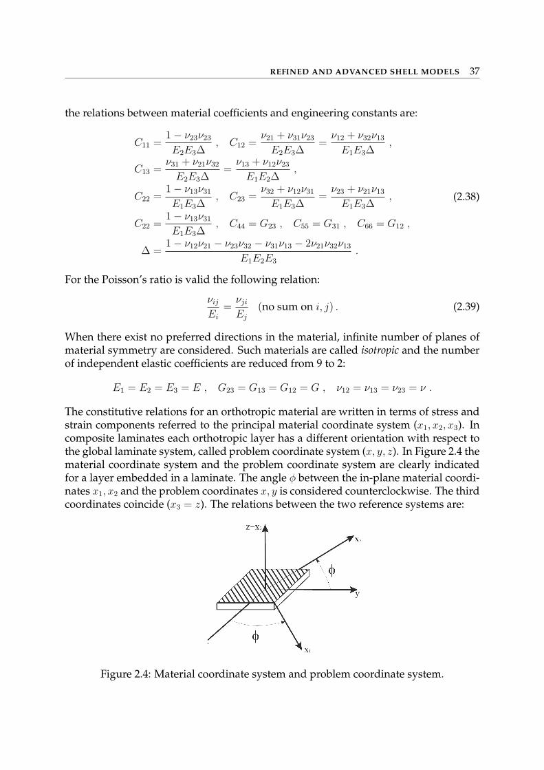
The constitutive relations for an orthotropic material are written in terms of stress andstrain components referred to the principal material coordinate system (x1, x2, x3). Incomposite laminates each orthotropic layer has a different orientation with respect tothe global laminate system, called problem coordinate system (x, y, z). In Figure 2.4 thematerial coordinate system and the problem coordinate system are clearly indicatedfor a layer embedded in a laminate. The angle φ between the in-plane material coordi-nates x1, x2 and the problem coordinates x, y is considered counterclockwise. The thirdcoordinates coincide (x3 = z). The relations between the two reference systems are:
Figure 2.4: Material coordinate system and problem coordinate system.
38 CHAPTER 2
x1
x2
x3
=
cos φ sin φ 0− sin φ cos φ 0
0 0 1
xyz
. (2.40)
Applying this rotation to the stress tensor σij and rearranging in terms of a single-column stress array, one obtains:
σxx
σyy
σzz
σyz
σxz
σxy
=
cos2 φ sin2 φ 0 0 0 − sin 2φsin2 φ cos2 φ 0 0 0 sin 2φ
0 0 1 0 0 00 0 0 cos φ sin φ 00 0 0 − sin φ cos φ 0
sin φ cos φ sin φ cos φ 0 0 0 cos2 φ− sin2 φ
σ11
σ22
σ33
σ23
σ13
σ12
. (2.41)
The equations (2.41) can be expressed in compact form as:
σp = [T ]σm , (2.42)
where p indicates quantities related to the problem reference system and m to the ma-terial reference system.The same procedure can be applied for the transformation of strain components, there-fore one has:
εm = [T ]Tεp . (2.43)
The only remaining quantities that need to be transformed from material coordinatesystem to the problem coordinates are the material parameters Cij . These can be easilyobtained considering the Eqs.(2.42) and (2.43):
σp = [T ]σm = σp = [T ][C]mεm = [T ][C]m[T ]Tεp = [C]pεp . (2.44)
[C]p is the material stiffness matrix in the problem coordinates and it can be rearrangedas in Eqs. (2.37).
The thickness locking (TL) mechanism, also known as Poisson’s locking phenomena,affects the plate/shell analysis [121],[122]. The TL doesn’t permit to an equivalent sin-gle layer theory with transverse displacement w constant or linear through the thick-ness (that means transverse strain εzz zero or constant) to lead to the 3D solution inthin plate/shell problems. A known technique to contrast TL consists in modifyingthe elastic stiffness coefficients by forcing the ’contradictory’ condition of transversenormal stress equal to zero:
σzz = 0 .
By imposing this condition in the constitutive equations (2.36), the modified stiff-ness coefficients in material reference system (reduced stiffness coefficients) can beobtained:
C11 =E1
1− ν12ν21
, C22 =E2
1− ν12ν21
, C12 =ν12E2
1− ν12ν21
. (2.45)
In order to avoid the TL, these coefficients must be used in [C]m in the place of C11, C22, C12
and then rotated according to Eq.(2.44).
REFINED AND ADVANCED SHELL MODELS 39
2.3.2 Multifield problems
Constitutive equations for the electro-thermo-mechanical problem can be obtained ac-cording to [129] and [130]. The coupling between the mechanical, thermal and electri-cal fields can be determined by using the thermodynamical principles and Maxwell’srelations [131]. For this aim, it is necessary to define a Gibbs free energy [132]. Formore details about the mathematical passages, one can refer to [129] and [130]. In thiswork, three particular cases are discussed: pure mechanical problem (seen in the pre-vious section); thermo-mechanical problem; electro-mechanical problem.In the case of thermo-mechanical problems, electrical loads are not applied on the struc-ture. The coupling between the mechanical and electrical fields, and between the ther-mal and electrical fields are not considered. The constitutive equations are:
σp = Cppεp + Cpnεn − λpθ ,
σn = Cnpεp + Cnnεn − λnθ ,
hp = κppϑp + κpnϑn ,
hn = κnpϑp + κnnϑn ,
(2.46)
where the variation of entropy is not considered because, in this work, the temperatureis imposed on the structure surfaces. While, the information about the heat flux h arefundamental to understand how the temperature profile evolves along the thicknessof the structure.The matrixes introduced are:
• Heat flux:
hp =
hα
hβ
, hn =
hz
. (2.47)
• Thermo-mechanical coupling coefficients:
λp =
λ1
λ2
λ6
, λn =
00λ3
. (2.48)
• Conductivity coefficients:
κpp =
[κ11 κ12
κ12 κ22
], κpn =
[00
],
κnp =[0 0
], κnn =
[κ33
].
(2.49)
In the case of electro-mechanical problem, two physical fields interact, no thermal loadsand spatial temperature gradients are applied on the structure. The couplings between
40 CHAPTER 2
mechanical and thermal fields, and between electrical and thermal fields are not con-sidered. In this case, the constitutive equations are:
σp = Cppεp + Cpnεn − eTppEp − eT
pnEn ,
σn = Cnpεp + Cnnεn − eTnpEp − eT
nnEn ,
Dp = eppεp + epnεn + εppEp + εpnEn ,
Dn = enpεp + ennεn + εnpEp + εnnEn .
(2.50)
The matrixes introduced are:
• Electrical displacement:
Dp =
Dα
Dβ
, Dn =
Dz
. (2.51)
• Piezoelectric coefficients:
epp =
[0 0 00 0 0
], epn =
[e15 e14 0e25 e24 0
],
enp =[e31 e32 e36
], enn =
[0 0 e33
].
(2.52)
• Permittivity coefficients:
εpp =
[ε11 ε12
ε12 ε22
], εpn =
[00
],
εnp =[0 0
], εnn =
[ε33
].
(2.53)
The meaning of these constitutive equations are clarified in next sections, where theopportune variational statements and governing equations are discussed.
2.3.3 Functionally graded materials
In the case of Functionally Graded Materials (FGMs), the properties change with con-tinuity along a particular direction of plate/shell, usually along the thickness. Thematrices of elastic coefficients, piezoelectric coefficients, thermo-mechanical couplingcoefficients and conductivity coefficients are general continuous functions of the thick-ness coordinate z (or ξ3).It is possible to describe the variation in z of the material properties via particularthickness functions that are a combination of Legendre polynomials (Eqs.(2.5)), that is:
C(z) = Fb(z)Cb + Fγ(z)Cγ + Ft(z)Ct ,
λ(z) = Fb(z)λb + Fγ(z)λγ + Ft(z)λt ,
κ(z) = Fb(z)κb + Fγ(z)κγ + Ft(z)κt ,
e(z) = Fb(z)eb + Fγ(z)eγ + Ft(z)et ,
ε(z) = Fb(z)εb + Fγ(z)εγ + Ft(z)εt .
(2.54)
REFINED AND ADVANCED SHELL MODELS 41
t and b are the top and bottom values. γ denotes the higher order terms of the expan-sion and it goes from 2 to 10, that is enough to guarantee a good approximation of theFGMs properties. The constants Cb, Cγ,Ct,λb... and so on, can be calculated knowingthe value of the related property in 10 different locations along the thickness. For moredetails, one can refer to [133] and [134].Alternatively, one can directly integrate the material properties as general function ofz. Since the thickness functions Fτ , Fs are arbitrary, the integrals in the thickness di-rection are numerically calculated in this work. For this reason, any function of thematerial properties can be integrated.
2.4 Variational statements
The variational statements considered in this work are the Principle of Virtual Dis-placements (PVD) and the Reissner’s Mixed Variational Theorem (RMVT). The PVDextended to thermo-electro-mechanical problems is easily obtained by considering thethermal, electrical and mechanical internal works and the opportune constitutive equa-tions. In this way, the use of Carrera’s Unified Formulation (CUF) permits to obtainseveral refined two-dimensional models. Particular cases of the PVD are simply ob-tained by discarding thermal, electrical or mechanical internal works. The extension ofthe RMVT to multifield problems is obtained by rearranging the constitutive equationsseen in the previous section and using opportune Lagrange multipliers in the varia-tional statement. Such two-dimensional models, obtained via the RMVT, are calledadvanced models.
2.4.1 Principle of Virtual Displacements
The Principle of Virtual Displacements in the general case of a thermo-electro-elasticproblem can be derived from the Hamilton’s principle as indicated in [129] and [130].Omitting the mathematical passages and neglecting the terms that are not involved inour problems, the final form of the PVD is the following:∫
V
(δεT
pGσpC +δεTnGσnC−δET
pGDpC−δETnGDnC−δϑT
pGhpC−δϑTnGhnC
)dV = δLe−δLin .
(2.55)V is the volume of the structure. Subscripts C and G suggest the substitution of consti-tutive and geometrical relations, respectively. T means the transpose of a vector and δthe virtual variation.δLe is the virtual variation of the work done by the external loads, that are mechanicalpu, thermal pθ and electrical pΦ. The explicit expression of the external work is:
δLe =
∫
V
(δu pu + δθ pθ + δΦ pΦ) dV , (2.56)
while the expression of the inertial work δLin is:
δLin =
∫
V
δu ρ u dV , (2.57)
42 CHAPTER 2
where ρ is the density of the material and double dots indicate the second temporalderivative.
In the case of pure mechanical problems, the PVD has only the displacement u asprimary variable and is simplified by discarding the internal thermal and electricalworks: ∫
V
(δεT
pGσpC + δεTnGσnC
)dV = δLe − δLin . (2.58)
In the case of thermo-mechanical problems, two approaches can be considered. If thetemperature is seen as an external load, it produces thermal stresses according to theconstitutive equations (2.46), but there is no heat flux produced by the mechanicalstrains. In this case, the PVD used is in the form of Eq.(2.58). If the coupling betweenthe thermal and mechanical fields is accounted, the PVD becomes the following:
∫
V
(δεT
pGσpC + δεTnGσnC − δϑT
pGhpC − δϑTnGhnC
)dV = δLe − δLin . (2.59)
In this work, only the first approach is considered.In the case of electro-mechanical coupling, for example the use of piezoelectric materi-als and/or the application of an electrical load, the relative PVD can be simply obtainedby discarding the internal thermal work:
∫
V
(δεT
pGσpC + δεTnGσnC − δET
pGDpC − δETnGDnC
)dV = δLe − δLin . (2.60)
For more details about this topic, one can refer to [128] and [129].
2.4.2 Reissner’s Mixed Variational Theorem
The Reissner’s Mixed Variational Theorem (RMVT) [63] permits to assume two inde-pendent sets of variables: a set of primary unknowns as the PVD case, and a set of ex-tensive variables which are modelled a priori in the thickness direction. The main ad-vantage of using the RMVT is a priori and complete fulfillment of the C0
z-requirementsfor the modelled extensive variables [81]. In this work, the RMTV is used only for theanalysis of pure-mechanical and electromechanical problems. Therefore, the thermalterms seen in the PVD will be discarded in the following equations.It is possible to obtain different extensions of RMVT by adding a Lagrange’s multiplierin the PVD for each extensive variable considered (transverse stresses, normal electricdisplacement and so on). When a new Lagrange’s multiplier is added [63], the con-stitutive equations must be rearranged in order to explicit the modelled variables. Forthis reason, each proposed extension of RMVT cannot be seen as a particular case of theother two. The extensive variables are modelled by means of the Unified Formulation(2.1). The approach in this case is always layer wise, independently on the modellingof the displacements (ESL or LW), because it permits to directly satisfy the interlaminarcontinuity conditions.
The first extension of RMVT, that can be considered, is the a-priori modelling ofthe transverse stresses σnM (the new subscript M is introduced to remark that the
REFINED AND ADVANCED SHELL MODELS 43
transverse stresses are now modelled and not obtained via constitutive equations). Theadded Lagrange’s multiplier is δσT
nM(εnG − εnC). The condition to add this multiplieris that the transverse strains εn calculated by means of geometrical relations (G) andby using the constitutive equations (C) must be the same or almost the same. In thisway the balance of the internal work does not change or remains almost the same.In the case of pure mechanical problems, the RMVT reads:
∫
V
(δεT
pGσpC + δεTnGσnM + δσT
nM(εnG − εnC))dV = δLe − δLin . (2.61)
The relative constitutive equations are obtained from Eqs.(2.36) considering the trans-verse stresses σnM as modelled and the transverse strains εnC as obtained from consti-tutive equations:
σp = Cppεp + Cpnσn ,
εn = Cnpεp + Cnnσn .(2.62)
The material coefficients are rearranged in the matrixes Cpp, Cpn, Cnp, Cnn in order toexpress εn in function of σn. If one considers also the contribution of the electrical field,the RMVT becomes:∫
V
(δεT
pGσpC + δεTnGσnM + δσT
nM(εnG − εnC)− δETpGDpC − δET
nGDnC
)dV = δLe − δLin ,
(2.63)and the constitutive equations (2.50) are modified as follows:
σp = Cppεp + Cpnσn + eTppEp + eT
pnEn ,
εn = Cnpεp + Cnnσn + eTnpEp + eT
nnEn ,
Dp = eppεp + epnσn + εppEp + εpnEn ,
Dn = enpεp + ennσn + εnpEp + εnnEn .
(2.64)
All the material coefficients, also the electrical ones, are recalculated.In the analysis of electro-mechanical problems, other transverse variables can be
modelled a priori, such as the transverse normal electric displacement Dz. So othertwo extensions of the RMVT are possible: - introduction of a new Lagrange’s multi-plier for the modelling of the transverse normal electric displacement; - introductionof two Lagrange’s multipliers for both transverse stresses and transverse normal elec-tric displacement. The first one cannot be considered a particular case of the secondone because the constitutive equations change.In the first case, the variational statement is:∫
V
(δεT
pGσpC + δεTnGσnC − δET
pGDpC − δETnGDnM − δDT
nM(EnG−EnC))dV = δLe− δLin ,
(2.65)
44 CHAPTER 2
the Lagrange’s multiplier δDTnM(EnG − EnC) has been added. The constitutive equa-
tions are re-written in function of Dn:
σp = Cppεp + Cpnεn + eTppEp + eT
pnDn ,
σn = Cnpεp + Cnnεn + eTnpEp + eT
nnDn ,
Dp = eppεp + epnεn + εppEp + εpnDn ,
En = enpεp + ennεn + εnpEp + εnnDn .
(2.66)
In the second case, both the Lagrange’s multipliers seen above are added:∫
V
(δεT
pGσpC + δεTnGσnM + δσT
nM(εnG − εnC)− δETpGDpC − δET
nGDnM − δDTnM(EnG − EnC)
)dV
= δLe − δLin ,
(2.67)
and the constitutive equations are:
σp = Cppεp + Cpnσn + eTppEp + eT
pnDn ,
εn = Cnpεp + Cnnσn + eTnpEp + eT
nnDn ,
Dp = eppεp + epnσn + εppEp + εpnDn ,
En = enpεp + ennσn + εnpEp + εnnDn .
(2.68)
One has to pay attention that the coefficients with the hat are not always the same, butthey must be derived for each variational statement. For more details about this topic,one can refer to [128] and [129].
2.5 Acronyms of CUF models
Several refined and advanced two-dimensional models are contained in the UnifiedFormulation. Depending on the variables description (LW, ESL or ZZ), the order ofexpansion in the thickness direction and the variational statement used, a large varietyof kinematics shell theories can be obtained. A system of acronyms is given in order todenote these models. The first letter indicates the multi-layer approach which can beEquivalent Single Layer (E) or Layer Wise (L). The second letter refers to the employedvariational statement: (D) for the Principle of Virtual Displacements and (M) for theReissner’s Mixed Variational Theorem. A number in the third position indicates the or-der of expansion (N) (from 1 to 4). In the case of ESL approach, a letter (Z) can be addedif the zig-zag effects of displacements are considered by means of Murakami’s zig-zagfunction. Summarizing, ED1-ED4 are ESL models based on PVD. If Murakami’s zigzagfunction is used, these models are indicated as EDZ1-EDZ3. Classical theories such asClassical Lamination Theory (CLT) and First order Shear Deformation Theory (FSDT),can be obtained as particular cases of ED1 theory simply imposing constant value ofthe transversal displacement through the thickness direction. An appropriate applica-tion of penalty technique to shear moduli of the material leads to CLT. In the case of

REFINED AND ADVANCED SHELL MODELS 45
layer wise approaches, the letter L is considered in place of E, so the acronyms are LD1-LD4. Finally, if the RMVT is used, the acronyms become: EM1-EM4 and LM1-LM4. Inthis case, the Murakami’s function is not applied. When the structure is made of onesingle layer, the ESL and LW approaches provide the same results, thus just the orderof expansion N will be indicated in the tables to distinguish the theories.

Chapter 3
Differential equations and solutionmethods
Anisotropy, nonlinear analysis as well as complicating effects, such as the C0z - Requirements
(zig-zag effects in the displacements and interlaminar continuity for the stresses), the couplingsbetween in-plane and out-of-plane strains, make the analysis of layered composite structurescomplicated in practice. Analytical, closed form solutions are available in very few cases. Inmost of the practical problems, the solution demand applications of approximated computationalmethods.In this work, an analytical method, that is the Navier method, and two approximated numer-ical methods, that are the Finite Element Method and the Radial Basis Functions method, areemployed to solve the governing equations of the problems considered. The Unified Formu-lation permits to derive the governing equations in terms of some few basic elements calledfundamental nuclei. Expanding them by means of opportune indexes and loops, it is possibleto obtain the stiffness matrix of the global structure. The use of such nuclei permits to obtainin a unified manner several refined and advanced models which differ for the order of expansionin the thickness direction, for the choice of the modelled multifield variables, and for the multi-layer description, ESL or LW. As an example, the PVD variational statement is here developedto obtain the differential equations for the analysis of multilayered structures. The governingequations can be obtained in weak form for the Finite Element Method or strong form for theNavier method or the Radial Basis Functions method. A review of these solution methods isalso provided, with particular attention to the finite element method that is the most commonmethod in literature and it is the main topic of this thesis.
3.1 Governing equations
In the case of pure mechanical problems, the Principle of Virtual Displacements (PVD)states as indicated in Eq.(2.58):
∫
V
(δεT
p σp + δεTnσn
)dV = δLe − δLin . (3.1)
47
48 CHAPTER 3
If the structure analyzed is a laminate of Nl layers, the integral on the volume Vk of ageneric layer k is split into an integral on the in-plane domain Ωk plus an integral inthe thickness domain Ak:
∫
Ωk
∫
Ak
(δεkT
p σkp + δεkT
n σkn
)H dΩk dAk = δLk
e − δLkin . (3.2)
where δLke and δLk
in are the external and the inertial virtual works at the k-layer level,respectively. The factor H has been introduced according to the Eqs.(2.33) (here cylin-drical geometry is considered). The relative constitutive equations are those obtainedin Eq.(2.36), but written for each layer k:
σkp = Ck
ppεkp + Ck
pnεkn ,
σkn = Ck
npεkp + Ck
nnεkn ,
(3.3)
By substituting the constitutive equations (3.3) in the variational statement (3.2), oneobtains:∫
Ωk
∫
Ak
(δεkT
p (Ckppε
kp + Ck
pnεkn) + δεkT
n (Cknpε
kp + Ck
nnεkn)
)H dΩk dξ3
k = δLke − δLk
in . (3.4)
The following step is the substitution of the geometrical relations of Eq.(2.22), writtenfor a generic layer k:
εkp =(Dk
p + Akp)u
k ,
εkn =(Dk
np + Dknz −Ak
n)uk ,(3.5)
in which the factor Hk (see Eqs.(2.23) and (2.24)) is calculated in two different ways:
• H = (1 + ξ3
R) if the variable description is equivalent single layer and it doesn’t
depend on the layer k;
• Hk = (1 + ζk
Rk ), where Rk is the curvature radius of the midsurface of the layer k,if the variable description is layer wise.
The same for the factors Hα and Hβ (see Eqs.(2.30) and (2.31)) in the case of double-curvature geometry. After the substitution of geometrical relations, one has:∫
Ωk
∫
Ak
(((Dk
p + Akp)δuk)T (Ck
pp(Dkp + Ak
p) + Ckpn(Dk
np + Dknz −Ak
n))uk+
((Dknp + Dk
nz −Akn)δuk)T (Ck
np(Dkp + Ak
p) + Cknn(Dk
np + Dknz −Ak
n))uk)H dΩk dξ3
k =
δLke − δLk
in .
(3.6)
Finally, the Unified Formulation is introduced, as in Eq.(2.1):
δuk = Fτδukτ , uk = Fsu
ks , τ, s = 0, 1, ..., N , (3.7)
DIFFERENTIAL EQUATIONS AND SOLUTION METHODS 49
where, in practice, the displacement u depends on k only if the approach is LW. Sub-stituting in the previous equation (3.6), one obtains the governing equations in weakform that are:∫
Ωk
∫
Ak
(((Dk
p + Akp)Fτδu
kτ )
T (Ckpp(D
kp + Ak
p) + Ckpn(Dk
np + Dknz −Ak
n))Fsuks+
((Dknp + Dk
nz −Akn)Fτδu
kτ )
T (Cknp(D
kp + Ak
p) + Cknn(Dk
np + Dknz −Ak
n))Fsuks
)H dΩk dξ3
k =
δLke − δLk
in .
(3.8)
At this step, it is possible to apply the Finite Element Method because the boundaryconditions are applied in weak form (more details will be provided below). While, ifthe Navier method or meshless methods, such as the Radial Basis Functions, are em-ployed to solve the governing equations, one needs to derive the equations in strongform. In this way, one has a set of differential equations on the domain Ωk, that arethe governing equations, and a set of equations on the edge Γk, that are the relativeboundary conditions.For this aim, the integration by part is used, that permits to move the differential oper-ators from the infinitesimal variation of the displacement δuk to the finite quantity uk.For a generic variable a, the integration by parts states:
∫
Ωk
((Dk
Ω)δak)T
akdΩk = −∫
Ωk
δakT ((DkT
Ω )ak)dΩk +
∫
Γk
δakT ((Ik
Ω)ak)dΓk (3.9)
where Ω = p, np. The matrix IΩ is obtained applying the Gradient theorem:∫
Ωk
∂ak
∂ξidΩk =
∮
Γk
niakdΓk (3.10)
in which ni are the components of the vector n, that is the normal to the boundary Γk,along the direction ξi.After integration by parts, the governing equations and the relative boundary condi-tions are obtained from Eq.(3.8):∫
Ωk
∫
Ak
δukTτ
((−Dk
p + Akp)
T (Ckpp(D
kp + Ak
p) + Ckpn(Dk
np + Dknz −Ak
n))+
(−Dknp + Dk
nz −Akn)T (Ck
np(Dkp + Ak
p) + Cknn(Dk
np + Dknz −Ak
n)))uk
sFτFs H dΩk dξ3k+∫
Γk
∫
Ak
δukTτ
(IkT
p (Ckpp(D
kp + Ak
p) + Ckpn(Dk
np + Dknz −Ak
n))+
IkTnp (Ck
np(Dkp + Ak
p) + Cknn(Dk
np + Dknz −Ak
n)))uk
sFτFs H dΓk dξ3k =∫
Ωk
∫
Ak
(δukTτ pu)Fτ H dΩk dξ3
k −∫
Ωk
∫
Ak
(δukTτ ρk uk
s)FτFs H dΩk dξ3k .
(3.11)
50 CHAPTER 3
The matrices to perform the integration by parts Ikp and Ik
np have the following form,in analogy with the matrices for the geometrical relations:
Ikp =
n1 0 00 n1 0n2 n1 0
, Ik
np =
0 0 n1
0 0 n2
0 0 0
. (3.12)
n1 and n2 are the components of the normal to the boundary of domain Ω that is:
n =
[n1
n2
]=
[cos(ϕ1)cos(ϕ2)
](3.13)
ϕ1 and ϕ2 are the angles between the normal n and the direction ξ1 and ξ2, respectively.Whether the Finite Element Method or the Navier and Radial Basis Functions methodsare applied, the final form of the governing equations is:
δukτ
T: Kkτs
uu uks = P k
uτ −M kτsuu uk
s (3.14)
In the case of strong form solution, one has also the related Neumann-type boundaryconditions on the edge Γk:
Πkτsuu uk
s = Πkτsuu uk
s , (3.15)
In these equations, Kkτsuu is the so-called fundamental nucleus for the stiffness matrix,
P kuτ is the vector of the external mechanical loads, M kτs
uu is the matrix of the inertialcontribution, written in form of fundamental nucleus, and Πkτs
uu is the fundamental nu-cleus for the boundary conditions. uk
s is the vector of degrees of freedom, uks is the
second temporal derivative of uks and uk
s is the vector of the displacements assigned onthe boundary.The stiffness matrix of each layer k is calculated by expanding the fundamental nu-cleus Kkτs
uu on the indexes τ and s. Then, the stiffness matrix of the global structure isobtained by assembling these matrices at multilayer level. Two different assemblingprocedures are used, depending on the variable description: if the approach is equiva-lent single layer, the assembling procedure is shown in Fig.3.1; if the approach is layerwise, the procedure is that of Fig.3.2.
3.2 Navier method
The Navier method permits to calculate the closed form solution of the governingequations under particular conditions of geometry, boundary and material. These con-ditions are:
• the geometry in the plane of the plate or shell must be rectangular;
• the structure must be simply supported on the boundary;
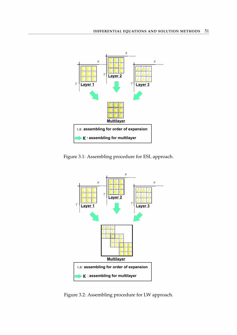
DIFFERENTIAL EQUATIONS AND SOLUTION METHODS 51
Figure 3.1: Assembling procedure for ESL approach.
Figure 3.2: Assembling procedure for LW approach.
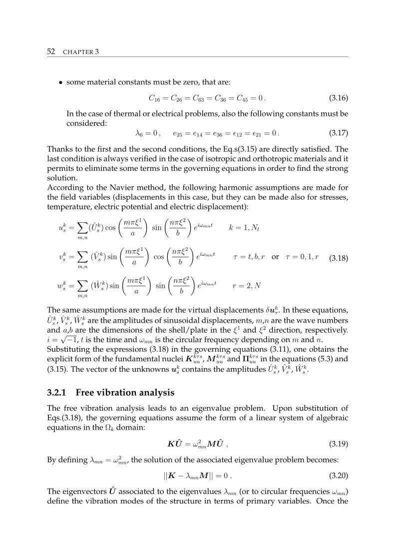
52 CHAPTER 3
• some material constants must be zero, that are:
C16 = C26 = C63 = C36 = C45 = 0 . (3.16)
In the case of thermal or electrical problems, also the following constants must beconsidered:
λ6 = 0 , e25 = e14 = e36 = ε12 = ε21 = 0 . (3.17)
Thanks to the first and the second conditions, the Eq.s(3.15) are directly satisfied. Thelast condition is always verified in the case of isotropic and orthotropic materials and itpermits to eliminate some terms in the governing equations in order to find the strongsolution.According to the Navier method, the following harmonic assumptions are made forthe field variables (displacements in this case, but they can be made also for stresses,temperature, electric potential and electric displacement):
uks =
∑m,n
(Uks ) cos
(mπξ1
a
)sin
(nπξ2
b
)eiωmnt k = 1, Nl
vks =
∑m,n
(V ks ) sin
(mπξ1
a
)cos
(nπξ2
b
)eiωmnt τ = t, b, r or τ = 0, 1, r
wks =
∑m,n
(W ks ) sin
(mπξ1
a
)sin
(nπξ2
b
)eiωmnt r = 2, N
(3.18)
The same assumptions are made for the virtual displacements δukτ . In these equations,
Uks , V k
s , W ks are the amplitudes of sinusoidal displacements, m,n are the wave numbers
and a,b are the dimensions of the shell/plate in the ξ1 and ξ2 direction, respectively.i =
√−1, t is the time and ωmn is the circular frequency depending on m and n.Substituting the expressions (3.18) in the governing equations (3.11), one obtains theexplicit form of the fundamental nuclei Kkτs
uu , M kτsuu and Πkτs
uu in the equations (5.3) and(3.15). The vector of the unknowns uk
s contains the amplitudes Uks , V k
s , W ks .
3.2.1 Free vibration analysis
The free vibration analysis leads to an eigenvalue problem. Upon substitution ofEqs.(3.18), the governing equations assume the form of a linear system of algebraicequations in the Ωk domain:
KU = ω2mnMU , (3.19)
By defining λmn = ω2mn, the solution of the associated eigenvalue problem becomes:
||K − λmnM || = 0 . (3.20)
The eigenvectors U associated to the eigenvalues λmn (or to circular frequencies ωmn)define the vibration modes of the structure in terms of primary variables. Once the
DIFFERENTIAL EQUATIONS AND SOLUTION METHODS 53
waves number (m,n) has been defined in the in-plane directions, the number of ob-tained frequencies becomes equal to the degrees of freedom of the employed two-dimensional model. It is possible to obtain the relative eigenvector, in terms of pri-mary variables, for each value of frequency, in order to obtain the modes plotted in thethickness direction.
3.3 Finite element method
Among the computational techniques implemented for the analysis of layered struc-tures, a predominant role has been played by Finite Element Method (FEM). The mostof the finite elements, available in literature, are formulated on the bases of axiomatic-type theories. According to MacNeal [135] the first FEM analysis was published in1961. The majority of early FEM calculations were performed with the classical Kirchhoff-Love theory and some examples are given in [136]-[140]. But, it was difficult to satisfythe requirements of compatibility in thin shell analysis because the rotations were de-rived from the transversal displacement. For this reason, plate/shell elements includ-ing classical transverse shear effects (FSDT) were developed by Pryor and Barker [141],Noor [142], Hughes [143], Panda and Natarayan [144], Parisch [145], Ferreira [146] andmany others. However, early FSDT type elements showed severe stiffening in thinplate/shell limits. Such a numerical mechanism, known as shear or membrane locking,was first contrasted by implementation of numerical tricks, such as reduced/selectiveintegration schemes [147]-[151]. But, spurious zero energy modes are introduced bythese sub-integration techniques. In [152] and [153], Chinosi et al. developed a hierar-chic finite element for thin Naghdi shell model [154] that was able to contrast lockingfor the shell problem in its displacement formulation. However, in the case of verysmall thickness and when the element is not of degree as high as needed, the numericalsolution exhibits a loss in the rate of convergence. The so-called Mixed Interpolationof Tensorial Components (MITC) was implemented to overcome both these problems.Many articles by Bathe and others are available on that topic: examples are the papers[155]-[160]. Arnold and Brezzi [161] dealt with a mixed formulation of the Naghdimodel, giving a family of locking free elements and proving the convergence of theirnumerical approach. Similarly, Ramm and Bischoff [162]-[166] developed a shell finiteelement based on a 7-parameter theory, in which the extra strain term is incorporatedvia the enhanced assumed strain concept proposed by Simo and Rafai [167].Also a large variety of plate/shell finite element implementations of higher-order theo-ries (HOT) have been proposed in the last twenty years literature. HOT-based C0 finiteelements (C0 means that the continuity is required only for the unknown variablesand not for their derivatives) were discussed by Kant and co-authors [168],[169]. In[170]-[174], Polit et al. proposed a C1 six-nodes triangular finite element in which thetransverse shear strains are represented by cosine functions. This element is able to en-sure both the continuity conditions for displacements and transverse shear stresses atthe interfaces between layers of laminated structures. A comprehensive discussion ofHOT-type theories and related finite element suitability has been provided by Tessler
54 CHAPTER 3
[175]. Many other papers are available in which HOTs have been implemented forplates and shells, details can be found in the books by Reddy [176] and Palazotto andDennis [177].Dozens of finite elements have been proposed based on zig-zag theories [178],[179].An application of Reissner Mixed Variational Theorem (RMVT) [180] to develop stan-dard finite elements was proposed by Rao and Meyer-Piening [181]. A generalizationof RMVT as a tool to develop approximate solutions was given by Carrera [26]. The ob-tained finite elements represent the FE implementation of the Murakami theory [123]and were denoted by the acronym RMZC, (Reissner Mindlin Zigzag interlaminar Con-tinuity). Full extensions of RMZC to shell geometries have been done by Brank andCarrera [182].Finite element implementations of layer-wise theories in the framework of axiomatic-type theories have been proposed by many authors, among which Noor and Burton[183], Reddy [184], Mawenya and Davies [185], Pinsky and Kim [186], Chaudhuri andSeide [189], Rammerstorfer et al. [188]. Finally, the finite element presented in thiswork is based on both equivalent-single-layer, zig-zag and layer-wise models con-tained in the CUF [81],[82],[127] and it employs the MITC method to contrast the mem-brane and shear locking.
3.3.1 CUF MITC9 shell element
According to the Finite Element Method (FEM), the displacement field (see Eqs.(2.1))is interpolated by means of the shape functions Ni, Nj :
δuk = FτNiδqkτi
, uk = FsNjqksj
, (3.21)
where τ, s = 0, 1, ..., N , i, j = 1, ..., Nn and Nn is the number of nodes of the element.qk
sjand δqk
τiare the nodal displacements and their virtual variations. The element
considered in this work has 9 nodes and the Lagrangian shape functions are used tointerpolate the displacements. These functions are obtained by imposing that Ni as-sumes the value 1 in the node i and 0 in the others, and they are expressed in the localreference system of the element (ξ, η) (see Figure 3.3), as follows:
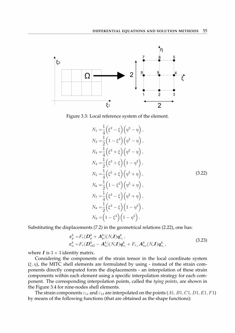
DIFFERENTIAL EQUATIONS AND SOLUTION METHODS 55
Ω
1
98
7 6 5
4
32
2
2
ξ
η
ξ1
ξ2
Figure 3.3: Local reference system of the element.
N1 =1
4
(ξ2 − ξ
)(η2 − η
),
N2 =1
2
(1− ξ2
)(η2 − η
),
N3 =1
4
(ξ2 + ξ
)(η2 − η
),
N4 =1
2
(ξ2 + ξ
)(1− η2
),
N5 =1
4
(ξ2 + ξ
)(η2 + η
),
N6 =1
2
(1− ξ2
)(η2 + η
),
N7 =1
4
(ξ2 − ξ
)(η2 + η
),
N8 =1
2
(ξ2 − ξ
)(1− η2
),
N9 =(1− ξ2
)(1− η2
).
(3.22)
Substituting the displacements (7.2) in the geometrical relations (2.22), one has:
εkp =Fτ (D
kp + Ak
p)(NiI)qkτi
,
εkn =Fτ (D
knΩ −Ak
n)(NiI)qkτi
+ Fτ,zAknz(NiI)qk
τi,
(3.23)
where I is 3× 3 identity matrix.Considering the components of the strain tensor in the local coordinate system
(ξ, η), the MITC shell elements are formulated by using - instead of the strain com-ponents directly computed form the displacements - an interpolation of these straincomponents within each element using a specific interpolation strategy for each com-ponent. The corresponding interpolation points, called the tying points, are shown inthe Figure 3.4 for nine-nodes shell elements.
The strain components ε11 and ε13 are interpolated on the points (A1, B1, C1, D1, E1, F1)by means of the following functions (that are obtained as the shape functions):
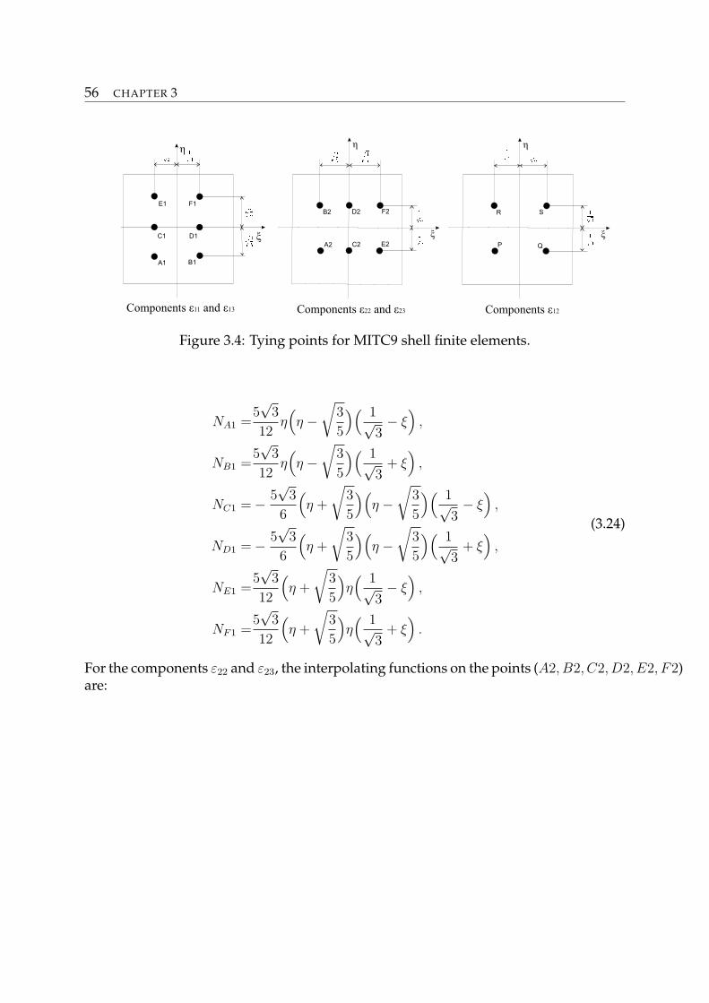
56 CHAPTER 3
ξ
η
A1
C1
E1 F1
D1
B1
Components andε ε22 23
ξ
η
A2
B2
C2
D2 F2
E2
ξ
η
P
R S
Q
Components andε ε11 13 Components ε12
Figure 3.4: Tying points for MITC9 shell finite elements.
NA1 =5√
3
12η(η −
√3
5
)( 1√3− ξ
),
NB1 =5√
3
12η(η −
√3
5
)( 1√3
+ ξ)
,
NC1 =− 5√
3
6
(η +
√3
5
)(η −
√3
5
)( 1√3− ξ
),
ND1 =− 5√
3
6
(η +
√3
5
)(η −
√3
5
)( 1√3
+ ξ)
,
NE1 =5√
3
12
(η +
√3
5
)η( 1√
3− ξ
),
NF1 =5√
3
12
(η +
√3
5
)η( 1√
3+ ξ
).
(3.24)
For the components ε22 and ε23, the interpolating functions on the points (A2, B2, C2, D2, E2, F2)are:
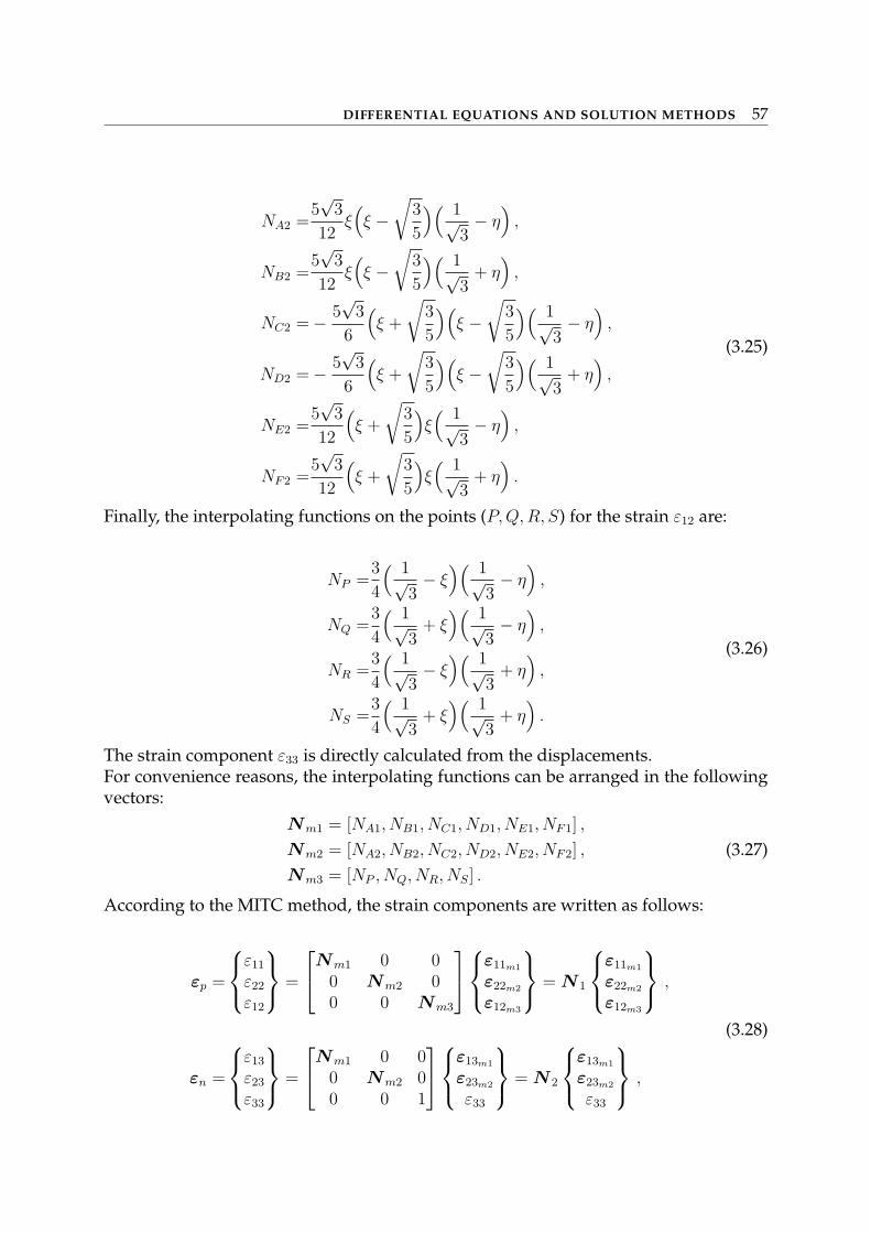
DIFFERENTIAL EQUATIONS AND SOLUTION METHODS 57
NA2 =5√
3
12ξ(ξ −
√3
5
)( 1√3− η
),
NB2 =5√
3
12ξ(ξ −
√3
5
)( 1√3
+ η)
,
NC2 =− 5√
3
6
(ξ +
√3
5
)(ξ −
√3
5
)( 1√3− η
),
ND2 =− 5√
3
6
(ξ +
√3
5
)(ξ −
√3
5
)( 1√3
+ η)
,
NE2 =5√
3
12
(ξ +
√3
5
)ξ( 1√
3− η
),
NF2 =5√
3
12
(ξ +
√3
5
)ξ( 1√
3+ η
).
(3.25)
Finally, the interpolating functions on the points (P, Q, R, S) for the strain ε12 are:
NP =3
4
( 1√3− ξ
)( 1√3− η
),
NQ =3
4
( 1√3
+ ξ)( 1√
3− η
),
NR =3
4
( 1√3− ξ
)( 1√3
+ η)
,
NS =3
4
( 1√3
+ ξ)( 1√
3+ η
).
(3.26)
The strain component ε33 is directly calculated from the displacements.For convenience reasons, the interpolating functions can be arranged in the followingvectors:
Nm1 = [NA1, NB1, NC1, ND1, NE1, NF1] ,
Nm2 = [NA2, NB2, NC2, ND2, NE2, NF2] ,
Nm3 = [NP , NQ, NR, NS] .
(3.27)
According to the MITC method, the strain components are written as follows:
εp =
ε11
ε22
ε12
=
Nm1 0 00 Nm2 00 0 Nm3
ε11m1
ε22m2
ε12m3
= N 1
ε11m1
ε22m2
ε12m3
,
εn =
ε13
ε23
ε33
=
Nm1 0 00 Nm2 00 0 1
ε13m1
ε23m2
ε33
= N 2
ε13m1
ε23m2
ε33
,
(3.28)
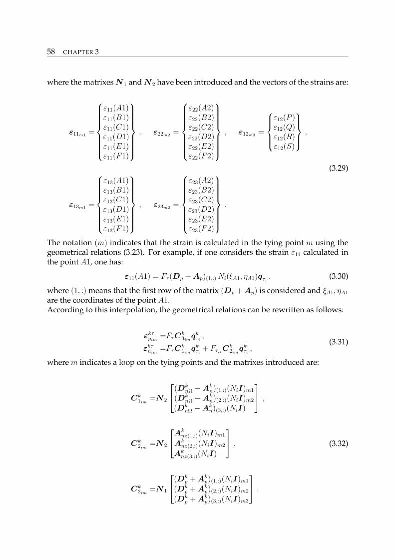
58 CHAPTER 3
where the matrixes N 1 and N 2 have been introduced and the vectors of the strains are:
ε11m1 =
ε11(A1)ε11(B1)ε11(C1)ε11(D1)ε11(E1)ε11(F1)
, ε22m2 =
ε22(A2)ε22(B2)ε22(C2)ε22(D2)ε22(E2)ε22(F2)
, ε12m3 =
ε12(P )ε12(Q)ε12(R)ε12(S)
,
ε13m1 =
ε13(A1)ε13(B1)ε13(C1)ε13(D1)ε13(E1)ε13(F1)
, ε23m2 =
ε23(A2)ε23(B2)ε23(C2)ε23(D2)ε23(E2)ε23(F2)
.
(3.29)
The notation (m) indicates that the strain is calculated in the tying point m using thegeometrical relations (3.23). For example, if one considers the strain ε11 calculated inthe point A1, one has:
ε11(A1) = Fτ (Dp + Ap)(1,:) Ni(ξA1, ηA1)qτi, (3.30)
where (1, :) means that the first row of the matrix (Dp + Ap) is considered and ξA1, ηA1
are the coordinates of the point A1.According to this interpolation, the geometrical relations can be rewritten as follows:
εkτpim
=FτCk3im
qkτi
,
εkτnim
=FτCk1im
qkτi
+ Fτ,zCk2im
qkτi
,(3.31)
where m indicates a loop on the tying points and the matrixes introduced are:
Ck1im
=N 2
(DknΩ −Ak
n)(1,:)(NiI)m1
(DknΩ −Ak
n)(2,:)(NiI)m2
(DknΩ −Ak
n)(3,:)(NiI)
,
Ck2im
=N 2
Aknz(1,:)(NiI)m1
Aknz(2,:)(NiI)m2
Aknz(3,:)(NiI)
,
Ck3im
=N 1
(Dkp + Ak
p)(1,:)(NiI)m1
(Dkp + Ak
p)(2,:)(NiI)m2
(Dkp + Ak
p)(3,:)(NiI)m3
.
(3.32)
DIFFERENTIAL EQUATIONS AND SOLUTION METHODS 59
Also the constitutive equations are rewritten considering the loop on the tying pointsby means of the index n:
σkspjn
=Ckppε
kspjn
+ Ckpnε
ksnjn
,
σksnjn
=Cknpε
kspjn
+ Cknnε
ksnjn
.(3.33)
By exploiting the constitutive equations (3.33), the geometrical relations (3.31) and thedisplacement field (7.2) in the PVD (3.2), one obtains:
δqkTτi
∫
Ak
Fτ
( ∫
Ωk
[CkT3im
(CkppC
k3jn
+ CkpnC
k1jn
) + CkT1im
(CknpC
k3jn
+ CknnC
k1jn
)]dΩk
)FsHk dξ3
k
qk
sj+
δqkTτi
∫
Ak
Fτ
( ∫
Ωk
[(CkT
3imCk
pn + CkT1im
Cknn)Ck
2jn
]dΩk
)Fs,3Hk dξ3
k
qk
sj+
δqkTτi
∫
Ak
Fτ,3
( ∫
Ωk
[CkT2im
(CknpC
k3jn
+ CknnCk
1jn)]dΩk
)FsHk dξ3
k
qk
sj+
δqkTτi
∫
Ak
Fτ,3
( ∫
Ωk
[CkT
2imCk
nnCk2jn
]dΩk
)Fs,3Hk dξ3
k
qk
sj=
δqkTτi
∫
Ak
Fτ
( ∫
Ωk
Nip dΩk
)Hk dξ3
k
,
(3.34)
Therefore, the following governing equation system is written:
δqkτi
: Kkτsijqksj
= P kτi
(3.35)
where the vector of unknowns is given by the nodal displacements qksj
and the funda-mental nucleus is dependent on the indexes i, j.
3.4 RBF collocation method
Recently, radial basis functions (RBFs) have enjoyed considerable success and researchas a technique for interpolating data and functions. A radial basis function, φ(‖x−xj‖)is a spline that depends on the Euclidian distance between distinct data centers xj, j =1, 2, ..., N ∈ Rn, also called nodal or collocation points. Although most work to dateon RBFs relates to scattered data approximation and in general to interpolation theory,there has recently been an increased interest in their use for solving partial differen-tial equations (PDEs). This approach, which approximates the whole solution of thePDE directly using RBFs, is truly a mesh-free technique. Kansa [190] introduced theconcept of solving PDEs by an unsymmetric RBF collocation method based upon theMulti Quadratic (MQ) interpolation functions, in which the shape parameter may varyacross the problem domain. The use of alternative methods to the Finite Element Meth-ods for the analysis of plates and shells, such as the meshless methods based on radial
60 CHAPTER 3
basis functions is atractive due to the absence of a mesh and the ease of collocationmethods. The use of radial basis function for the analysis of structures and materialshas been previously studied by numerous authors [191]-[204].Radial basis functions (RBF) approximations are mesh-free numerical schemes that canexploit accurate representations of the boundary, are easy to implement and can bespectrally accurate. In this section, the formulation of a global unsymmetrical colloca-tion RBF-based method to compute elliptic operators is presented.The radial basis function (φ) approximation of a function (u) is given by:
u(x) =N∑
i=1
αiφ (‖x− yi‖2) , x ∈ Rn , (3.36)
where yi, i = 1, .., N is a finite set of distinct points (centers) in Rn. The most commonRBFs are:
Cubic: φ(r) = r3 ,
Thin plate splines: φ(r) = r2 log(r) ,
Wendland functions: φ(r) = (1− r)m+p(r) ,
Gaussian: φ(r) = e−(cr)2 ,
Multiquadrics: φ(r) =√
c2 + r2 ,
Inverse Multiquadrics: φ(r) = (c2 + r2)−1/2 ,
where the Euclidian distance r is real and non-negative and c is a positive shape param-eter. Hardy [205] introduced multiquadrics in the analysis of scattered geographicaldata. In the 1990’s Kansa [190] used multiquadrics for the solution of partial differentialequations. Considering N distinct interpolations, and knowing u(xj), j = 1, 2, ..., N , αi
are found by the solution of a N ×N linear system:
Aα = u , (3.37)
where A = [φ (‖x− yi‖2)]N×N , α = [α1, α2, ..., αN ]T and u = [u(x1), u(x2), ..., u(xN)]T .
3.4.1 The static problem
Consider a linear elliptic partial differential operator L and a bounded region Ω inRn with some boundary ∂Ω. In the static problems, one seeks the computation ofdisplacements (u) from the global system of equations:
Lu = f in Ω , (3.38)
LBu = g on ∂Ω , (3.39)
DIFFERENTIAL EQUATIONS AND SOLUTION METHODS 61
where L, LB are linear operators in the domain and on the boundary, respectively. Theright-hand side of (3.38) and (3.39) represent the external forces applied on the shelland the boundary conditions applied along the perimeter of the shell, respectively. ThePDE problem defined in (3.38) and (3.39) will be replaced by a finite problem, definedby an algebraic system of equations, after the radial basis expansions.The solution of a static problem by radial basis functions considers NI nodes in thedomain and NB nodes on the boundary, with a total number of nodes N = NI + NB.The sampling points are denoted by xi ∈ Ω, i = 1, ..., NI and xi ∈ ∂Ω, i = NI + 1, ..., N .At the points in the domain, the following system of equations is solved:
N∑i=1
αiLφ (‖x− yi‖2) = f(xj), j = 1, 2, ..., NI , (3.40)
or:LIα = F , (3.41)
where:LI = [Lφ (‖x− yi‖2)]NI×N . (3.42)
At the points on the boundary, one can impose the boundary conditions as:
N∑i=1
αiLBφ (‖x− yi‖2) = g(xj), j = NI + 1, ..., N , (3.43)
or:Bα = G , (3.44)
where:B = LBφ [(‖xNI+1 − yj‖2)]NB×N .
Therefore, one can write a finite-dimensional static problem as:[ LI
B
]α =
[FG
]. (3.45)
By inverting the system (3.45), one obtains the vector α. Then, the solution u is ob-tained using the interpolation equation (3.36).The radial basis collocation method follows a simple implementation procedure. Tak-ing equation (3.11), one computes:
α =
[LI
B
]−1 [FG
]. (3.46)
This α vector is then used to obtain solution u, by using (2.1). If derivatives of u areneeded, such derivatives are computed as:
∂u∂x
=N∑
j=1
αj∂φj
∂x, (3.47)
62 CHAPTER 3
∂2u∂x2
=N∑
j=1
αj∂2φj
∂x2, etc . (3.48)
In the present collocation approach, one needs to impose essential and natural bound-ary conditions. Consider, for example, the condition w = 0, on a simply supported orclamped edge. The conditions are enforced by interpolating as:
w = 0 →N∑
j=1
αWj φj = 0 . (3.49)
Other boundary conditions are interpolated in a similar way.
3.4.2 The eigenproblem
The eigenproblem looks for eigenvalues (λ) and eigenvectors (u) that satisfy:
Lu + λu = 0 in Ω , (3.50)
LBu = 0 on ∂Ω . (3.51)
As in the static problem, the eigenproblem defined in (3.50) and (3.51) is replaced bya finite-dimensional eigenvalue problem, based on RBF approximations. NI nodesin the interior of the domain and NB nodes on the boundary are considered, withN = NI + NB. The interpolation points are denoted by xi ∈ Ω, i = 1, ..., NI and xi ∈∂Ω, i = NI + 1, ..., N . At the points in the domain, one can define the eigenproblem as:
N∑i=1
αiLφ (‖x− yi‖2) = λu(xj), j = 1, 2, ..., NI , (3.52)
or:LIα = λuI
, (3.53)
where:LI = [Lφ (‖x− yi‖2)]NI×N . (3.54)
At the points on the boundary, the boundary conditions are enforced as:
N∑i=1
αiLBφ (‖x− yi‖2) = 0, j = NI + 1, ..., N , (3.55)
or:Bα = 0 . (3.56)
Equations (3.53) and (3.56) can now be solved as a generalized eigenvalue problem:[ LI
B
]α = λ
[AI
0
]α , (3.57)
DIFFERENTIAL EQUATIONS AND SOLUTION METHODS 63
where:AI = φ [(‖xNI
− yj‖2)]NI×N .
For free vibration problems, the external force is set to zero, and the solution is assumedharmonic in terms of displacements uτ , uτ , wτ , as:
uτ = Uτ (w, y)eiωt , vτ = Vτ (w, y)eiωt , wτ = Wτ (w, y)eiωt , (3.58)
where ω is the frequency of natural vibration. Substituting the harmonic expansioninto equations (3.57) in terms of the amplitudes Uτ , Vτ ,Wτ , one can obtain the naturalfrequencies and vibration modes for the shell problem, by solving the eigenproblem:
[L − ω2G]X = 0 , (3.59)
where L collects all stiffness terms and G collects all terms related to the inertial terms.In (3.59) X are the modes of vibration associated with the natural frequencies definedas ω.

Chapter 4
Analytical solutions
This chapter discusses the analysis of some shell structures performed by means of the Naviermethod. First, the thermo-mechanical static analysis of functionally graded shells is considered.Here, the temperature profile along the thickness is not assumed but it is calculated by solvingthe Fourier’s heat conduction equation. Then, shell structures that include piezoelectric layersare analyzed. Only the free vibration analysis is performed and particular attention is given tothe effect of the electro-mechanical coupling on the solution. Finally, the dynamic analysis of adouble-walled carbon nanotube is presented. In this case, an equivalent continuum shell modelis formulated in the framework of the CUF, that permits to take into account the van der Waalsinteraction between the tubes. Different models contained in the CUF, refined and advanced,are used for these analyses and the capability of each model to reproduce the quasi-3D results isevaluated. Note that, in this chapter, every calculation is made referring to the double-curvaturegeometry and relative notation (see Section 2.2.1), even when the shell is cylindrical.
4.1 Thermo-mechanical analysis of FGM shells
In the present analysis, the temperature is seen as an external load. If the values of thetemperature are known at the top and bottom surface of the plate, the thermal load canbe considered in two different ways. The first method introduces an assumed profileT (z) that varies linearly from the top to the bottom; the second one computes T (z) bysolving Fourier’s heat conduction equation [210]. In this paper only the second way isconsidered because even for a very thin FGM layer the temperature profile is nonlinear.Therefore, the assumption of a linear T (z) would cause very large errors.The temperature profile is described in the same way as the displacements in case ofthe Layer Wise approach:
T k(α, β, z) = Fτ θkτ with τ = t, b, l and l = 2, . . . , 14 , (4.1)
The thickness functions Fτ are a combination of Legendre polynomials.In general, for the kth homogeneous orthotropic layer, the differential Fourier’s equa-tion of heat conduction reads:
(Kk1
H2α
) ∂2T
∂α2+
(Kk2
H2β
) ∂2T
∂β2+ Kk
3
∂2T
∂z2= 0 . (4.2)
65
66 CHAPTER 4
The coefficients Kk1 , Kk
2 and Kk3 depend on z because some layers k can be in FGM.
In case of shell we can define three new coefficients K∗k1 =
Kk1 (z)
H2α
, K∗k2 =
Kk2 (z)
H2β
and
K∗k3 = Kk
3 (z), which in a generic layer k depend on the thickness coordinate of theshell. K∗k
1 and K∗k2 can depend by the thickness coordinate z for two reasons: possible
use of FGM layers and/or presence of curvature in case of shells; K∗k3 can depend by z
coordinate only in case of FGM layers. So Fourier’s equation becomes:
K∗k1
∂2T
∂α2+ K∗k
2
∂2T
∂β2+ K∗k
3
∂2T
∂z2= 0 . (4.3)
The Eq.(4.3) has not constant coefficients in the layer k. It can be solved by introducing,for each layer k, a given number of mathematical layers (Nml) in which K∗k
1 , K∗k2 and
K∗k3 can be supposed constant. In each mathematical layer, the values of Hα and Hβ
and the material properties of the FGM layer can be calculated at a given value of thecoordinate z, so the mean value between the values at the top and bottom of mathe-matical layer is taken for Kj
1 , Kj2 and Kj
3 , while the value at the midsurface is takenfor Hα and Hβ . The complete procedure to calculate the temperature profile T(z) andto obtain the values of θk
τ for the Eq.(4.1) is reported in [211], where the plate case isconsidered, but the Fourier’s equation is formally the same (K∗k
1 = Kk1 , K∗k
2 = Kk2 and
K∗k3 = Kk
3 for the plate).
4.1.1 Governing equations
The procedure to obtain the governing equations is that exposed in the previous chap-ter (Section 3.1) for the closed form solution. Substituting the geometrical relations(Eqs.(2.29)) and the constitutive equations (Eqs.(2.46 without considering the heat fluxh) in the variational statement (Eq.2.58), one obtains the following differential equi-librium equations, for a FGM multi-layered shell subjected to thermal and mechanicalloadings:
δuks
T: Kkτsr
uu ukτ = Kkτsr
uθ θkτ + P k
uτ , (4.4)
where (Kkτsruθ θk
τ ) is the thermal load. In this analysis, the material properties of FGMlayers are written using the Legendre polynomials (see Eqs.(2.54)).In order to apply the Navier method, the harmonic assumptions of Eqs.3.18 are madefor the displacements and for the temperature one has:
θks =
∑m,n
(θks ) sin
(mπαk
ak
)sin
(nπβk
bk
). (4.5)
Therefore, the explicit expressions of fundamental nuclei Kkτsruu and Kkτsr
uθ are:
ANALYTICAL SOLUTIONS 67
• Kuu
Kuu11 = Ck55J
kτzszrαβ +
1
Rkα
Ck55(−Jkτzsr
β − Jkτszrβ +
1
Rkα
Jkτsrβ/α ) + Ck
11Jkτsrβ/α α2 + Ck
66Jkτsrα/β β2 ,
Kuu12 = Jkτsrαβ(Ck12 + Ck
66) = Kuu21 ,
Kuu13 = Ck55(J
kτzsrβ α− 1
Rkα
Jkτsrβ/α α)− Ck
13Jkτszrβ α− 1
Rkα
Ck11J
kτsrβ/α α− Ck
12Jkτsrα
1
Rkβ
,
Kuu22 = Ck44J
kτzszrαβ +
1
Rkβ
Ck44(−Jkτzsr
α − Jkτszrα +
1
Rkβ
Jkτsrα/β ) + Ck
22Jkτsrα/β β2 + Ck
66Jkτsrβ/α α2 ,
Kuu23 = Ck44(J
kτzsrα β − 1
Rkβ
Jkτsrα/β β)− Ck
23Jkτszrα β − 1
Rkβ
Ck22J
kτsrα/β β − 1
Rkα
Ck12J
kτsrβ ,
Kuu31 = Ck55J
kτszrβ α− Ck
55
1
Rkα
Jkτsrβ/α α− Ck
13Jkτzsrβ α− 1
Rkα
Ck11J
kτsrβ/α α− 1
Rkβ
Ck12J
kτsrα ,
Kuu32 = Ck44(J
kτszrα β − 1
Rkβ
Jkτsrα/β β)− Ck
23Jkτzsrα β − 1
Rkβ
Ck22J
kτsrα/β β − 1
Rkα
Ck12J
kτsrβ ,
Kuu33 = Ck55J
kτsrβ/α α2 + Ck
44Jkτsrα/β β2 + Ck
33Jkτzszrαβ +
1
Rkα
(1
Rkα
Ck11J
kτsrβ/α + Ck
13Jkτszrβ + Ck
13Jkτzsrβ ) ,
+2
RkαRk
β
JkτsrCk12 +
1
Rkβ
(1
Rkβ
Ck22J
kτsrα/β + Ck
23Jkτzsrα + Ck
23Jkτszrα ) ,
• Kuθ
Kuθ1 = αJkτsrβ λk
p1 ,
Kuθ2 = βJkτsrα λk
p2 ,
Kuθ3 = − Jkτsrβ
1
Rkα
λkp1 − Jkτsr
α
1
Rkβ
λkp2 − Jkτzsr
αβ λkn3 ,
68 CHAPTER 4
where the following notation is introduced:
(Jkτsr, Jkτsrα , Jkτsr
β , Jkτsrαβ
, Jkτsrβα
, Jkτsrαβ ) =
∫
Ak
FrFτFs
(1, Hk
α, Hkβ ,
Hkα
Hkβ
,Hk
β
Hkα
, HkαHk
β
)dz ,
(Jkτzsr, Jkτzsrα , Jkτzsr
β , Jkτzsrαβ
, Jkτzsrβα
, Jkτzsrαβ ) =
∫
Ak
Fr∂Fτ
∂zFs
(1, Hk
α, Hkβ ,
Hkα
Hkβ
,Hk
β
Hkα
, HkαHk
β
)dz ,
(Jkτszr, Jkτszrα , Jkτszr
β , Jkτszrαβ
, Jkτszrβα
, Jkτszrαβ ) =
∫
Ak
FrFτ∂Fs
∂z
(1, Hk
α, Hkβ ,
Hkα
Hkβ
,Hk
β
Hkα
, HkαHk
β
)dz ,
(Jkτzszr, Jkτzszrα , Jkτzszr
β , Jkτzszrαβ
, Jkτzszrβα
, Jkτzszrαβ ) =
∫
Ak
Fr∂Fτ
∂z
∂Fs
∂z
(1, Hk
α, Hkβ ,
Hkα
Hkβ
,Hk
β
Hkα
, HkαHk
β
)dz ,
and α = mπ/a, β = nπ/b.If θk
τ = 0 in Eq.(5.3), only a mechanical load is considered. Vice versa, if P kuτ = 0, only
a thermal load is applied. The fundamental nuclei are formally the same in case of"classical" or FGM layers, the only difference is the assembling loop on index r whichaccounts for the variation of the material properties through the thickness.
4.1.2 Results and discussion
In this section a shell comprising a single functionally graded layer, is analyzed. Thegeometry is given by Ren: Rα →∞, Rβ = 10m, span angle in β-direction φ = π/3, a =1m. As a typical example for high-temperature applications, the constituent materialsof the functionally graded shell are taken to be Monel (70Ni-30Cu), a nickel-based alloy,and the ceramic zirconia (ZrO2). The required material properties are those reportedin [212]:
Bm = 227.24 GPa, µm = 65.55 GPa, αm = 15× 10−6 / K, Km = 25 W/mK, for Monel,
Bc = 125.83 GPa, µc = 58.08 GPa, αc = 10× 10−6 / K, Kc = 2.09 W/mK, for zirconia.
For this two-phase composite material different micromechanical models can be ap-plied for the computation of the effective local material properties. According to [212],the following formulas are chosen:
• The effective bulk modulus B and shear modulus µ are given by the mean fieldestimate of Mori and Tanaka [213],[214]:
B −Bm
Bc −Bm
=V2
1 + (1− V2)Bc−Bm
Bm+ 43µm
, (4.6)
µ− µm
µc − µm
=V2
1 + (1− V2)µc−µm
µm+f1
, with f1 =µm(9Bm + 8µm)
6(Bm + 2µm). (4.7)
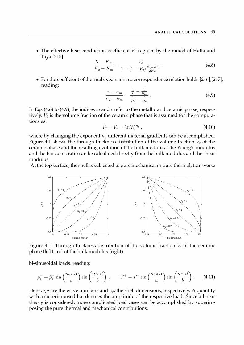
ANALYTICAL SOLUTIONS 69
• The effective heat conduction coefficient K is given by the model of Hatta andTaya [215]:
K −Km
Kc −Km
=V2
1 + (1− V2)Kc−Km
3Km
. (4.8)
• For the coefficient of thermal expansion α a correspondence relation holds [216],[217],reading:
α− αm
αc − αm
=1B− 1
Bm
1Bc− 1
Bm
. (4.9)
In Eqs.(4.6) to (4.9), the indices m and c refer to the metallic and ceramic phase, respec-tively. V2 is the volume fraction of the ceramic phase that is assumed for the computa-tions as:
V2 = Vc = (z/h)ng , (4.10)
where by changing the exponent ng different material gradients can be accomplished.Figure 4.1 shows the through-thickness distribution of the volume fraction Vc of theceramic phase and the resulting evolution of the bulk modulus. The Young’s modulusand the Poisson’s ratio can be calculated directly from the bulk modulus and the shearmodulus.At the top surface, the shell is subjected to pure mechanical or pure thermal, transverse
-0.5
-0.25
0
0.25
0.5
0 0.25 0.5 0.75 1
z / h
volume fraction
ng = 5
ng = 2
ng = 1
ng = 0.5
ng = 0.2
-0.5
-0.25
0
0.25
0.5
125 150 175 200 225
z / h
bulk modulus
ng = 5
ng = 2
ng = 1
ng = 0.5
ng = 0.2
Figure 4.1: Through-thickness distribution of the volume fraction Vc of the ceramicphase (left) and of the bulk modulus (right).
bi-sinusoidal loads, reading:
p+z = p+
z sin(mπ α
a
)sin
(n π β
b
), T+ = T+ sin
(mπ α
a
)sin
(nπ β
b
). (4.11)
Here m,n are the wave numbers and a,b the shell dimensions, respectively. A quantitywith a superimposed hat denotes the amplitude of the respective load. Since a lineartheory is considered, more complicated load cases can be accomplished by superim-posing the pure thermal and mechanical contributions.
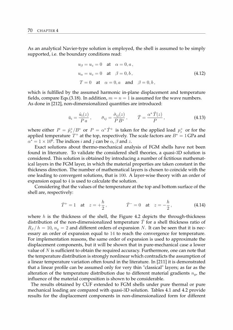
70 CHAPTER 4
As an analytical Navier-type solution is employed, the shell is assumed to be simplysupported, i.e. the boundary conditions read:
uβ = uz = 0 at α = 0, a ,
uα = uz = 0 at β = 0, b ,
T = 0 at α = 0, a and β = 0, b ,
(4.12)
which is fulfilled by the assumed harmonic in-plane displacement and temperaturefields, compare Eqs.(3.18). In addition, m = n = 1 is assumed for the wave numbers.As done in [212], non-dimensionalized quantities are introduced:
ui =ui(z)
P a, σij =
σij(z)
P B∗ , T =α∗ T (z)
P, (4.13)
where either P = p+z /B∗ or P = α∗ T+ is taken for the applied load p+
z or for theapplied temperature T+ at the top, respectively. The scale factors are B∗ = 1 GPa andα∗ = 1× 10⁶. The indices i and j can be α, β and z.
Exact solutions about thermo-mechanical analysis of FGM shells have not beenfound in literature. To validate the considered shell theories, a quasi-3D solution isconsidered. This solution is obtained by introducing a number of fictitious mathemat-ical layers in the FGM layer, in which the material properties are taken constant in thethickness direction. The number of mathematical layers is chosen to coincide with theone leading to convergent solutions, that is 100. A layer-wise theory with an order ofexpansion equal to 4 is used to calculate the solution.
Considering that the values of the temperature at the top and bottom surface of theshell are, respectively:
T+ = 1 at z = +h
2, T− = 0 at z = −h
2, (4.14)
where h is the thickness of the shell, the Figure 4.2 depicts the through-thicknessdistribution of the non-dimensionalized temperature T for a shell thickness ratio ofRβ / h = 10, ng = 2 and different orders of expansion N . It can be seen that it is nec-essary an order of expansion equal to 14 to reach the convergence for temperature.For implementation reasons, the same order of expansion is used to approximate thedisplacement components, but it will be shown that in pure-mechanical case a lowervalue of N is sufficient to obtain the required accuracy. Furthermore, one can note thatthe temperature distribution is strongly nonlinear which contradicts the assumption ofa linear temperature variation often found in the literature. In [211] it is demonstratedthat a linear profile can be assumed only for very thin "classical" layers; as far as thealteration of the temperature distribution due to different material gradients ng, theinfluence of the material composition is shown to be considerable.
The results obtained by CUF extended to FGM shells under pure thermal or puremechanical loading are compared with quasi-3D solution. Tables 4.1 and 4.2 provideresults for the displacement components in non-dimensionalized form for different
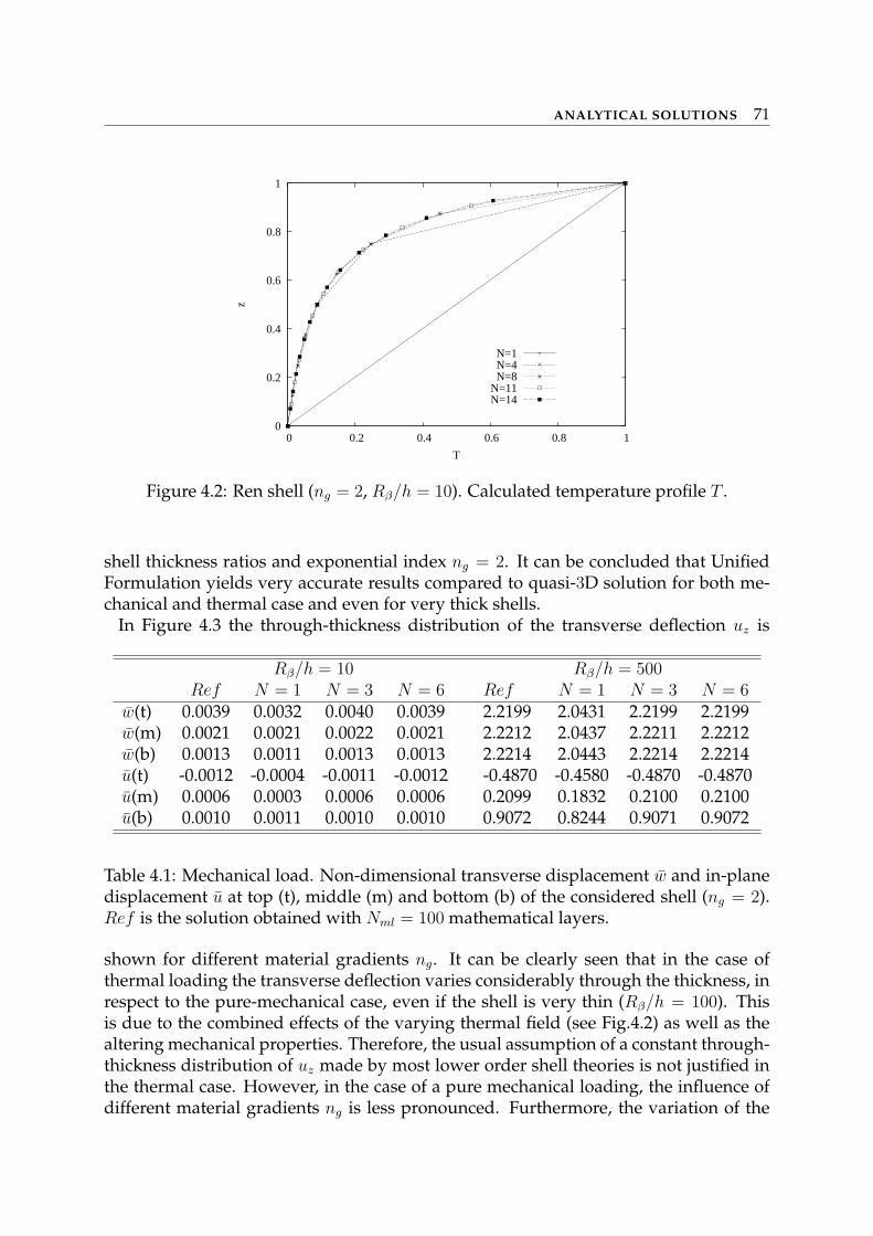
ANALYTICAL SOLUTIONS 71
0
0.2
0.4
0.6
0.8
1
0 0.2 0.4 0.6 0.8 1
z
T
N=1N=4N=8
N=11N=14
Figure 4.2: Ren shell (ng = 2, Rβ/h = 10). Calculated temperature profile T .
shell thickness ratios and exponential index ng = 2. It can be concluded that UnifiedFormulation yields very accurate results compared to quasi-3D solution for both me-chanical and thermal case and even for very thick shells.
In Figure 4.3 the through-thickness distribution of the transverse deflection uz is
Rβ/h = 10 Rβ/h = 500Ref N = 1 N = 3 N = 6 Ref N = 1 N = 3 N = 6
w(t) 0.0039 0.0032 0.0040 0.0039 2.2199 2.0431 2.2199 2.2199w(m) 0.0021 0.0021 0.0022 0.0021 2.2212 2.0437 2.2211 2.2212w(b) 0.0013 0.0011 0.0013 0.0013 2.2214 2.0443 2.2214 2.2214u(t) -0.0012 -0.0004 -0.0011 -0.0012 -0.4870 -0.4580 -0.4870 -0.4870u(m) 0.0006 0.0003 0.0006 0.0006 0.2099 0.1832 0.2100 0.2100u(b) 0.0010 0.0011 0.0010 0.0010 0.9072 0.8244 0.9071 0.9072
Table 4.1: Mechanical load. Non-dimensional transverse displacement w and in-planedisplacement u at top (t), middle (m) and bottom (b) of the considered shell (ng = 2).Ref is the solution obtained with Nml = 100 mathematical layers.
shown for different material gradients ng. It can be clearly seen that in the case ofthermal loading the transverse deflection varies considerably through the thickness, inrespect to the pure-mechanical case, even if the shell is very thin (Rβ/h = 100). Thisis due to the combined effects of the varying thermal field (see Fig.4.2) as well as thealtering mechanical properties. Therefore, the usual assumption of a constant through-thickness distribution of uz made by most lower order shell theories is not justified inthe thermal case. However, in the case of a pure mechanical loading, the influence ofdifferent material gradients ng is less pronounced. Furthermore, the variation of the
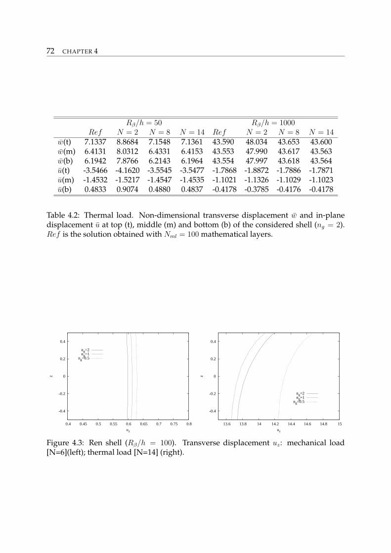
72 CHAPTER 4
Rβ/h = 50 Rβ/h = 1000Ref N = 2 N = 8 N = 14 Ref N = 2 N = 8 N = 14
w(t) 7.1337 8.8684 7.1548 7.1361 43.590 48.034 43.653 43.600w(m) 6.4131 8.0312 6.4331 6.4153 43.553 47.990 43.617 43.563w(b) 6.1942 7.8766 6.2143 6.1964 43.554 47.997 43.618 43.564u(t) -3.5466 -4.1620 -3.5545 -3.5477 -1.7868 -1.8872 -1.7886 -1.7871u(m) -1.4532 -1.5217 -1.4547 -1.4535 -1.1021 -1.1326 -1.1029 -1.1023u(b) 0.4833 0.9074 0.4880 0.4837 -0.4178 -0.3785 -0.4176 -0.4178
Table 4.2: Thermal load. Non-dimensional transverse displacement w and in-planedisplacement u at top (t), middle (m) and bottom (b) of the considered shell (ng = 2).Ref is the solution obtained with Nml = 100 mathematical layers.
-0.4
-0.2
0
0.2
0.4
0.4 0.45 0.5 0.55 0.6 0.65 0.7 0.75 0.8
z
uz
ng=2ng=1
ng=0.5
-0.4
-0.2
0
0.2
0.4
13.6 13.8 14 14.2 14.4 14.6 14.8 15
z
uz
ng=2ng=1
ng=0.5
Figure 4.3: Ren shell (Rβ/h = 100). Transverse displacement uz: mechanical load[N=6](left); thermal load [N=14] (right).
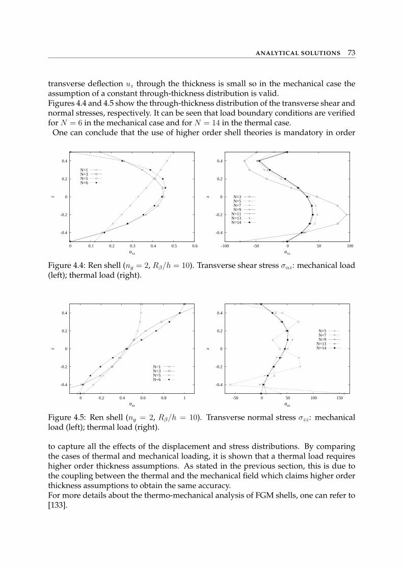
ANALYTICAL SOLUTIONS 73
transverse deflection uz through the thickness is small so in the mechanical case theassumption of a constant through-thickness distribution is valid.Figures 4.4 and 4.5 show the through-thickness distribution of the transverse shear andnormal stresses, respectively. It can be seen that load boundary conditions are verifiedfor N = 6 in the mechanical case and for N = 14 in the thermal case.
One can conclude that the use of higher order shell theories is mandatory in order
-0.4
-0.2
0
0.2
0.4
0 0.1 0.2 0.3 0.4 0.5 0.6
z
σxz
N=1N=3N=5N=6
-0.4
-0.2
0
0.2
0.4
-100 -50 0 50 100
z
σxz
N=3N=5N=7N=9
N=11N=13N=14
Figure 4.4: Ren shell (ng = 2, Rβ/h = 10). Transverse shear stress σαz: mechanical load(left); thermal load (right).
-0.4
-0.2
0
0.2
0.4
0 0.2 0.4 0.6 0.8 1
z
σzz
N=1N=3N=5N=6
-0.4
-0.2
0
0.2
0.4
-50 0 50 100 150
z
σzz
N=5N=7N=9
N=13N=14
Figure 4.5: Ren shell (ng = 2, Rβ/h = 10). Transverse normal stress σzz: mechanicalload (left); thermal load (right).
to capture all the effects of the displacement and stress distributions. By comparingthe cases of thermal and mechanical loading, it is shown that a thermal load requireshigher order thickness assumptions. As stated in the previous section, this is due tothe coupling between the thermal and the mechanical field which claims higher orderthickness assumptions to obtain the same accuracy.For more details about the thermo-mechanical analysis of FGM shells, one can refer to[133].
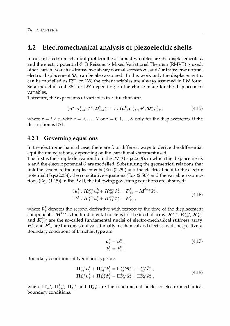
74 CHAPTER 4
4.2 Electromechanical analysis of piezoelectric shells
In case of electro-mechanical problem the assumed variables are the displacements uand the electric potential Φ. If Reissner’s Mixed Variational Theorem (RMVT) is used,other variables such as transverse shear/normal stresses σn and/or transverse normalelectric displacement Dn can be also assumed. In this work only the displacement ucan be modelled as ESL or LW, the other variables are always assumed in LW form.So a model is said ESL or LW depending on the choice made for the displacementvariables.Therefore, the expansions of variables in z direction are:
(uk,σknM , Φk,Dk
nM) = Fτ (uk, σknM , Φk, Dk
nM)τ , (4.15)
where τ = t, b, r, with r = 2, . . . , N or τ = 0, 1, ..., N only for the displacements, if thedescription is ESL.
4.2.1 Governing equations
In the electro-mechanical case, there are four different ways to derive the differentialequilibrium equations, depending on the variational statement used.The first is the simple derivation from the PVD (Eq.(2.60)), in which the displacementsu and the electric potential Φ are modelled. Substituting the geometrical relations thatlink the strains to the displacements (Eqs.(2.29)) and the electrical field to the electricpotential (Eqs.(2.35)), the constitutive equations (Eqs.(2.50)) and the variable assump-tions (Eqs.(4.15)) in the PVD, the following governing equations are obtained:
δuks : Kkτs
uu ukτ + Kkτs
uΦ Φkτ = P k
us −M kτsukτ ,
δΦks : Kkτs
Φu ukτ + Kkτs
ΦΦ Φkτ = P k
Φs ,(4.16)
where ukτ denotes the second derivative with respect to the time of the displacement
components. M kτs is the fundamental nucleus for the inertial array. Kkτsuu , Kkτs
uΦ , KkτsΦu
and KkτsΦΦ are the so-called fundamental nuclei of electro-mechanical stiffness array.
P kus and P k
Φs are the consistent variationally mechanical and electric loads, respectively.Boundary conditions of Dirichlet type are:
ukτ = uk
τ , (4.17)
Φkτ = Φk
τ ,
Boundary conditions of Neumann type are:
Πkτsuu uk
τ + ΠkτsuΦ Φk
τ = Πkτsuu uk
τ + ΠkτsuΦ Φk
τ ,
ΠkτsΦu uk
τ + ΠkτsΦΦ Φk
τ = ΠkτsΦu uk
τ + ΠkτsΦΦ Φk
τ ,(4.18)
where Πkτsuu , Πkτs
uΦ , ΠkτsΦu and Πkτs
ΦΦ are the fundamental nuclei of electro-mechanicalboundary conditions.
ANALYTICAL SOLUTIONS 75
Another way to derive the governing equations is the use of the RMVT (Eq.(2.63)) inwhich the stresses σn are modelled with the displacements and the electric potential.Substituting the geometrical relations (Eqs.(2.29) and (2.35)) and the modified consti-tutive equations (Eqs.(2.64)) in the Eq.(2.63), one has:
δuks : Kkτs
uu ukτ + Kkτs
uσ σknτ + Kkτs
uΦ Φkτ = P k
us −M kτsukτ ,
δσkns : Kkτs
σu ukτ + Kkτs
σσ σknτ + Kkτs
σΦ Φkτ = 0 ,
δΦks : Kkτs
Φu ukτ + Kkτs
Φσ σknτ + Kkτs
ΦΦ Φkτ = P k
Φs .
(4.19)
Nine fundamental nuclei are obtained which are completely different from those ob-tained from the PVD.Corresponding boundary conditions of Dirichlet type are:
ukτ = uk
τ , (4.20)
Φkτ = Φk
τ ,
while the Neumann ones are:
Πkτsuu uk
τ + Πkτsuσ σk
nτ + ΠkτsuΦ Φk
τ = Πkτsuu uk
τ + Πkτsuσ σk
nτ + ΠkτsuΦ Φk
τ ,
ΠkτsΦu uk
τ + ΠkτsΦσ σk
nτ + ΠkτsΦΦ Φk
τ = ΠkτsΦu uk
τ + ΠkτsΦσ σk
nτ + ΠkτsΦΦ Φk
τ .(4.21)
It is possible to conveniently model a priori the transverse normal electric displacementDz in the place of transverse stresses by using the RMVT in the form of Eq.(2.65). In thiscase, the governing equations, obtained by substituting in Eq.(2.65) the geometricalrelations (Eqs.(2.29) and (2.35)) and the modified constitutive equations (Eqs.(2.66)),read:
δuks : Kkτs
uu ukτ + Kkτs
uDDknτ + Kkτs
uΦ Φkτ = P k
us −M kτsukτ ,
δDkns : Kkτs
Du ukτ + Kkτs
DDDknτ + Kkτs
DΦΦkτ = 0 ,
δΦks : Kkτs
Φu ukτ + Kkτs
ΦDDknτ + Kkτs
ΦΦ Φkτ = P k
Φs .
(4.22)
Corresponding boundary conditions of Dirichlet type are:
uks = uk
s , (4.23)
Φks = Φk
s ,
the corresponding Neumann ones are:
Πkτsuu uk
τ + ΠkτsuDDk
nτ + ΠkτsuΦ Φk
τ = Πkτsuu uk
τ + ΠkτsuD Dk
nτ + ΠkτsuΦ Φk
τ ,
ΠkτsΦu uk
τ + ΠkτsΦDDk
nτ + ΠkτsΦΦ Φk
τ = ΠkτsΦu uk
τ + ΠkτsΦDDk
nτ + ΠkτsΦΦ Φk
τ .(4.24)
Finally, one can decide to model a priori both the transverse stresses and the transversenormal electric displacement and the governing equations can be derived from theRMVT in the form of Eqs.(2.67), substituting the geometrical relations (Eqs.(2.29) and
76 CHAPTER 4
(2.35)) and the modified constitutive equations (Eqs.(2.68)). In this case, the equationsare:
δuks : Kkτs
uu ukτ + Kkτs
uσ σknτ + Kkτs
uΦ Φkτ + Kkτs
uDDknτ = P k
us −M kτsukτ ,
δσkns : Kkτs
σu ukτ + Kkτs
σσ σknτ + Kkτs
σΦ Φkτ + Kkτs
σDDknτ = 0 ,
δΦks : Kkτs
Φu ukτ + Kkτs
Φσ σknτ + Kkτs
ΦΦ Φkτ + Kkτs
ΦDDknτ = P k
Φs ,
δDkns : Kkτs
Du ukτ + Kkτs
Dσ σknτ + Kkτs
DΦΦkτ + Kkτs
DDDknτ = 0 .
(4.25)
Dirichlet type boundary conditions are:
ukτ = uk
τ , (4.26)
Φkτ = Φk
τ ,
the Neumann ones are:
Πkτsuu uk
τ + Πkτsuσ σk
nMτ + ΠkτsuΦ Φk
τ + ΠkτsuD Dk
nMτ = Πkτsuu uk
τ + Πkτsuσ σk
nMτ
+ ΠkτsuΦ Φk
τ + ΠkτsuD Dk
nMτ ,
ΠkτsΦu uk
τ + ΠkτsΦσ σk
nMτ + ΠkτsΦΦ Φk
τ + ΠkτsΦD Dk
nMτ = ΠkτsΦu uk
τ + ΠkτsΦσ σk
nMτ
+ ΠkτsΦΦ Φk
τ + ΠkτsΦD Dk
nMτ .
(4.27)
In all the cases, the inertial array has the following expression:
M kτs =
∫
Ak
IρkFτFsHkαHk
β dz , (4.28)
where ρk is the mass density for each layer k, and I is the identity matrix of dimension[3×3].
Navier-type closed form solutions are applied to the proposed governing equationsand the following harmonic assumptions can be made for the field variables:
(ukατ
, σkαzτ
) =∑
m,n(Ukατ
, Skαzτ
) cos mπαk
aksin nπβk
bkeiωmn t , k = 1, Nl
(ukβτ
, σkβzτ
) =∑
m,n (Ukβτ
, Skβzτ
) sin mπαk
akcos nπβk
bkeiωmn t , τ = t, b, r
(ukzτ
, σkzzτ
, Φkτ ,Dk
nτ) =
∑m,n (Uk
zτ, Sk
zzτ, Φk
τ , Dknτ
) sin mπαk
aksin nπβk
bkeiωmn t , r = 2, N
(4.29)
in which the quantities with ˆ indicate the amplitudes. These assumptions correspondto the simply-supported boundary conditions. Upon substitution of Eq.(4.29), the gov-erning equations on Ωk assume the form of a linear system of algebraic equations inthe domain while the boundary conditions are exactly fulfilled. For the sake of brevity,the explicit expression of all the fundamental nuclei in closed-algebraic form is hereomitted but it can be found in [98].In the electromechanical case, the free vibration analysis leads to the following eigen-value problem:
K∗U = ω2mnMU , (4.30)
ANALYTICAL SOLUTIONS 77
where K∗ is the equivalent stiffness matrix obtained by means of static condensation(for further details see [218], [219]). Only the free vibration analysis is investigated inthis work and the external loadings (mechanical and electrical) are therefore set to zeroand the relative boundary conditions are exactly fulfilled.
4.2.2 Results and discussion
The free vibrations problem for multilayered shells including piezoelectric layers hasbeen investigated. By imposing the waves number in the in-plane directions, the cor-responding vibration modes are obtained. The number of frequencies is equal to thenumber of degrees of freedom through the thickness according to the considered kine-matics.
For the analysis, a multilayered ring shell is investigated. The geometry of the ringis given in Figure 4.6. The free vibrations problem is investigated by considering theclosed circuit configuration (Φt = Φb = 0). The elastic and piezoelectric properties ofthe employed materials and the geometrical parameters are given in Table 4.3.
The cylindrical ring shell is made of two layers, an internal layer in Titanium andan external one in piezoelectric PZT-4 with a thickness that is 1/4 of the total thick-ness. The free dimensional solution for this case is given by Heyliger et alii [220]:the first fundamental frequency in Hz (f = ω
2π) is given by imposing m = 0 and
n = 4, 8, 12, 16, 20. The thickness ratio is a constant and it is around 70.Table 4.4 gives the first fundamental frequencies in the case of CLT and FSDT. Tables 4.5and 4.6 consider the ESL models and the ESL models with the Murakami zigzag func-tion in the case of PVD extended to an electro-mechanical problem (PVD(u,Φ)). LWtheories are investigated in Table 4.7 using the same variational statement (PVD(u,Φ)).Tables 4.8-4.13 give the results of the first fundamental frequencies in the case of thethree possible extensions of RMVT to the electro-mechanical case; the same kinematicsmodels introduced for the PVD case are considered.
The results obtained in all cases (ESL or LW and PVD or RMVT model) are veryclose to the 3D solution if higher orders of expansion are used, the maximum erroris 2.68%. When lower orders of expansion are employed, if the variational statementis PVD, ESL models gives smaller errors than LW ones; if the variational statementis RMVT one has the opposite situation. In general, the error doesn’t depend on thewave number because by varying n one obtain completely different modes of vibra-tion. Table 4.4 shows that classical theories, such as CLT and FSDT, don’t give verylarge errors but the results are not so near to the 3D solution as in the other cases. Theuse of mixed models does not appear mandatory to obtain the frequencies: the kine-matic based PVD leads to a quasi-3D evaluation of the first fundamental frequenciesfor every wave number n. The use of mixed models instead appears mandatory to ob-tain the correct evaluation of modes through the thickness in terms of displacements,stresses, electric potential and electric displacement. This fact is illustrated in the fol-lowing analysis.The mode through the thickness for the fundamental frequency is given in Figs.(4.7)-(4.10) in terms of displacements, stresses, electric potential and electric displacement.
78 CHAPTER 4
The distribution of the transverse displacement uz through the thickness is given inFig.(4.7); in this case, there are no differences for the considered variational statementsbecause the displacement is a primary variable in all them. The mode is given inFig.(4.8) in terms of electric potential. The potential Φ consists of a primary variablein each considered model; as a consequence, the same considerations made for the dis-placements are confirmed: the electric potential is continuous and satisfies the closed-circuit boundary conditions. In order to give the mode through the thickness in termsof stress σzz, the use of mixed models in which σzz is a primary variable is mandatory:these models permit the interlaminar continuity and the correct boundary homoge-neous conditions to be obtained (see Fig.(4.9)). Finally, Fig.(4.10) gives the modes interms of transverse normal electric displacement Dz. As in the case of stress σzz, mixedmodels, where normal electric displacement is a primary variable, are necessary in or-der to achieve the interlaminar continuity of Dz at the interfaces.
The frequencies calculated using a pure mechanical model are quoted in Table 4.14.In order to estimate the piezoelectric effect, the following parameter is evaluated:
∆p[%] =
√ω2 − ω2
el
ω2· 100 , (4.31)
where the eigenfrequency ω is obtained by considering the electric effect, whereasωel is computed neglecting the electric part (only the elastic properties of the piezo-electric layers are considered). Due to the employed high orders of expansion, eachmodel gives the same value of the parameter ∆p, this is quite large so we can concludethat in this particulare case the electrical effect can’t be neglected. In addition to whatdemonstrated in [98] (the effect produced by the electromechanical interaction is notpredictable and does not depend on the thickness ratio and the order of the consideredmode), one can note that the parameter ∆p doesn’t depend on the wave number n.For more details about the electromechanical analysis of piezoelectric shells, one canrefer to [98].
4.3 Dynamic analysis of Double Walled Carbon Nanotubes(DWNT)
It has been demonstrated by Aydogdu [221] that single-beam continuum models, whichare often used in literature to study CNTs, can not represent the behavior of individ-ual tubes in a MWNT and relative deformation between adjacent tubes, because theyassume that all the originally concentric tubes of a MWNT remain coaxial during vi-bration. Therefore, refined MWNTs models are needed, in which also van der Waals(vdW) forces must be taken into consideration and which consider interlayer radialdisplacements and individual deflection curves of nested tubes within the MWNT.In this work, the discrete DWNT is considered as an equivalent continuum cylindri-cal shell composed of two adjacent layers (see Fig.4.11). As multi-beam models, CUF
ANALYTICAL SOLUTIONS 79
permits to consider each tube of the DWNT as independent by simply modifying theassembling procedure of the stiffness matrix on the layer k, as shown in Figure 4.12. Inthis way, the condition of continuity for the displacements at the layer interface is notfulfilled and the inner and outer tubes can vibrate separately.
In order to apply a continuum model for the free vibration analysis of the DWNTis necessary to determine its equivalent mechanical properties. In literature, there aremany dissenting opinions about the mechanical characterization of carbon nanotubes.This work is directed to validate the refined shell theories contained in CUF for theanalysis of DWNTs. According to [221] the effective wall thickness of the single carbonnanotube t is assumed to be equal to the interplanar spacing of graphite layers (0.35nm) and the mechanical properties are consequently calculated. The diameters of theinner and the outer walls of the double-walled nanotube are taken as d1 = 0.7 nm andd2 = 1.4 nm, respectively (see Fig.4.11). Young’s modulus and the shear modulus ofdouble-walled carbon nano tubes are assumed to be approximately insensitive to tubechirality. For the present DWNT and tube geometry, each tube is assumed to have thesame Young’s modulus of 1 TPa, shear modulus of 0.4 TPa, Poisson ratio of 0.25, andmass density of 2.3 g/cm3 with the effective thickness of 0.35 nm.
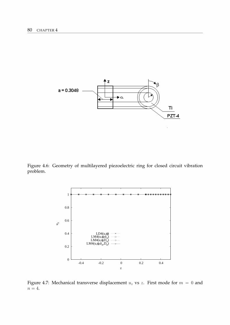
80 CHAPTER 4
Figure 4.6: Geometry of multilayered piezoelectric ring for closed circuit vibrationproblem.
0
0.2
0.4
0.6
0.8
1
-0.4 -0.2 0 0.2 0.4
u z
z
LD4(u,φ)LM4(u,φ,σn)LM4(u,φ,Dn)
LM4(u,φ,σn,Dn)
Figure 4.7: Mechanical transverse displacement uz vs z. First mode for m = 0 andn = 4.
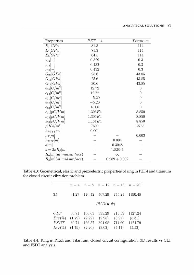
ANALYTICAL SOLUTIONS 81
Properties PZT − 4 TitaniumE1[GPa] 81.3 114E2[GPa] 81.3 114E3[GPa] 64.5 114ν12[−] 0.329 0.3ν13[−] 0.432 0.3ν23[−] 0.432 0.3G23[GPa] 25.6 43.85G13[GPa] 25.6 43.85G12[GPa] 30.6 43.85e15[C/m2] 12.72 0e24[C/m2] 12.72 0e31[C/m2] −5.20 0e32[C/m2] −5.20 0e33[C/m2] 15.08 0ε11[pC/V m] 1.306E4 8.850ε22[pC/V m] 1.306E4 8.850ε33[pC/V m] 1.151E4 8.850ρ[Kg/m3] 7600 2768hPZT4[m] 0.001 − −hT [m] − − 0.003hTOT [m] − 0.004 −a[m] − 0.3048 −b = 2πRβ[m] − 1.82841 −Rα[m](at midsurface) − ∞ −Rβ[m](at midsurface) − 0.289 + 0.002 −
Table 4.3: Geometrical, elastic and piezoelectric properties of ring in PZT4 and titaniumfor closed circuit vibration problem.
n = 4 n = 8 n = 12 n = 16 n = 20
3D 31.27 170.42 407.29 745.21 1190.48
PV D(u, Φ)
CLT 30.71 166.63 395.29 715.59 1127.24Err(%) (1.79) (2.22) (2.95) (3.97) (5.31)FSDT 30.71 166.57 394.98 714.60 1124.79Err(%) (1.79) (2.26) (3.02) (4.11) (5.52)
Table 4.4: Ring in PTZ4 and Titanium, closed circuit configuration. 3D results vs CLTand FSDT analysis.
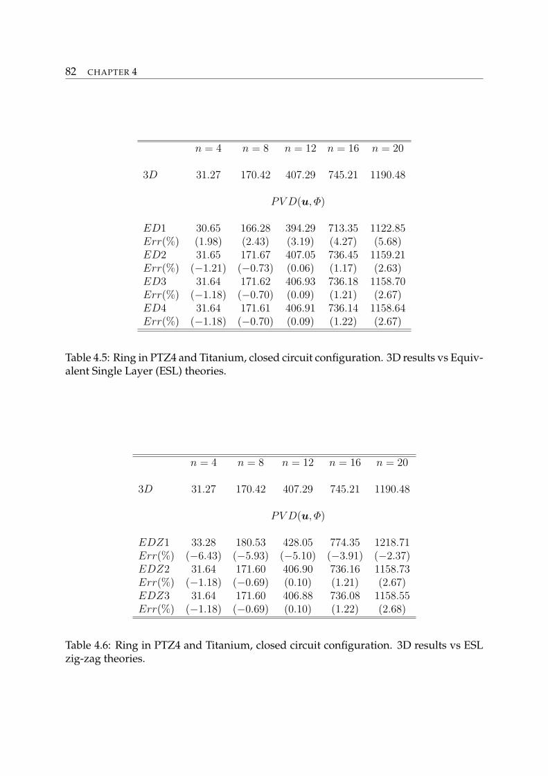
82 CHAPTER 4
n = 4 n = 8 n = 12 n = 16 n = 20
3D 31.27 170.42 407.29 745.21 1190.48
PV D(u, Φ)
ED1 30.65 166.28 394.29 713.35 1122.85Err(%) (1.98) (2.43) (3.19) (4.27) (5.68)ED2 31.65 171.67 407.05 736.45 1159.21Err(%) (−1.21) (−0.73) (0.06) (1.17) (2.63)ED3 31.64 171.62 406.93 736.18 1158.70Err(%) (−1.18) (−0.70) (0.09) (1.21) (2.67)ED4 31.64 171.61 406.91 736.14 1158.64Err(%) (−1.18) (−0.70) (0.09) (1.22) (2.67)
Table 4.5: Ring in PTZ4 and Titanium, closed circuit configuration. 3D results vs Equiv-alent Single Layer (ESL) theories.
n = 4 n = 8 n = 12 n = 16 n = 20
3D 31.27 170.42 407.29 745.21 1190.48
PV D(u, Φ)
EDZ1 33.28 180.53 428.05 774.35 1218.71Err(%) (−6.43) (−5.93) (−5.10) (−3.91) (−2.37)EDZ2 31.64 171.60 406.90 736.16 1158.73Err(%) (−1.18) (−0.69) (0.10) (1.21) (2.67)EDZ3 31.64 171.60 406.88 736.08 1158.55Err(%) (−1.18) (−0.69) (0.10) (1.22) (2.68)
Table 4.6: Ring in PTZ4 and Titanium, closed circuit configuration. 3D results vs ESLzig-zag theories.
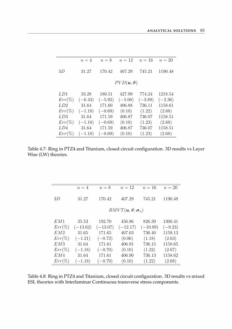
ANALYTICAL SOLUTIONS 83
n = 4 n = 8 n = 12 n = 16 n = 20
3D 31.27 170.42 407.29 745.21 1190.48
PV D(u, Φ)
LD1 33.28 180.51 427.99 774.24 1218.54Err(%) (−6.43) (−5.92) (−5.08) (−3.89) (−2.36)LD2 31.64 171.60 406.88 736.11 1158.61Err(%) (−1.18) (−0.69) (0.10) (1.22) (2.68)LD3 31.64 171.59 406.87 736.07 1158.51Err(%) (−1.18) (−0.69) (0.10) (1.23) (2.68)LD4 31.64 171.59 406.87 736.07 1158.51Err(%) (−1.18) (−0.69) (0.10) (1.23) (2.68)
Table 4.7: Ring in PTZ4 and Titanium, closed circuit configuration. 3D results vs LayerWise (LW) theories.
n = 4 n = 8 n = 12 n = 16 n = 20
3D 31.27 170.42 407.29 745.21 1190.48
RMV T (u, Φ, σn)
EM1 35.53 192.70 456.86 826.39 1300.41Err(%) (−13.62) (−13.07) (−12.17) (−10.89) (−9.23)EM2 31.65 171.65 407.03 736.40 1159.13Err(%) (−1.21) (−0.72) (0.06) (1.18) (2.63)EM3 31.64 171.61 406.91 736.15 1158.65Err(%) (−1.18) (−0.70) (0.10) (1.22) (2.67)EM4 31.64 171.61 406.90 736.13 1158.62Err(%) (−1.18) (−0.70) (0.10) (1.22) (2.68)
Table 4.8: Ring in PTZ4 and Titanium, closed circuit configuration. 3D results vs mixedESL theories with Interlaminar Continuous transverse stress components.
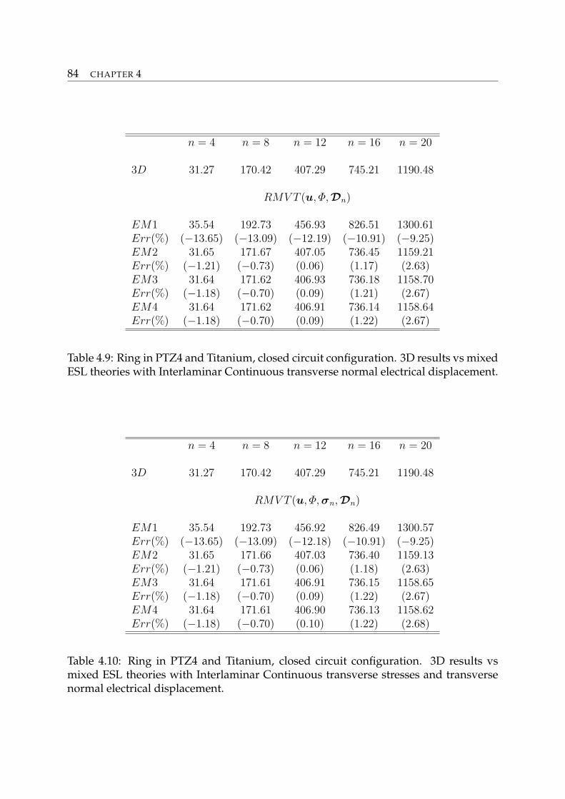
84 CHAPTER 4
n = 4 n = 8 n = 12 n = 16 n = 20
3D 31.27 170.42 407.29 745.21 1190.48
RMV T (u, Φ, Dn)
EM1 35.54 192.73 456.93 826.51 1300.61Err(%) (−13.65) (−13.09) (−12.19) (−10.91) (−9.25)EM2 31.65 171.67 407.05 736.45 1159.21Err(%) (−1.21) (−0.73) (0.06) (1.17) (2.63)EM3 31.64 171.62 406.93 736.18 1158.70Err(%) (−1.18) (−0.70) (0.09) (1.21) (2.67)EM4 31.64 171.62 406.91 736.14 1158.64Err(%) (−1.18) (−0.70) (0.09) (1.22) (2.67)
Table 4.9: Ring in PTZ4 and Titanium, closed circuit configuration. 3D results vs mixedESL theories with Interlaminar Continuous transverse normal electrical displacement.
n = 4 n = 8 n = 12 n = 16 n = 20
3D 31.27 170.42 407.29 745.21 1190.48
RMV T (u, Φ, σn,Dn)
EM1 35.54 192.73 456.92 826.49 1300.57Err(%) (−13.65) (−13.09) (−12.18) (−10.91) (−9.25)EM2 31.65 171.66 407.03 736.40 1159.13Err(%) (−1.21) (−0.73) (0.06) (1.18) (2.63)EM3 31.64 171.61 406.91 736.15 1158.65Err(%) (−1.18) (−0.70) (0.09) (1.22) (2.67)EM4 31.64 171.61 406.90 736.13 1158.62Err(%) (−1.18) (−0.70) (0.10) (1.22) (2.68)
Table 4.10: Ring in PTZ4 and Titanium, closed circuit configuration. 3D results vsmixed ESL theories with Interlaminar Continuous transverse stresses and transversenormal electrical displacement.
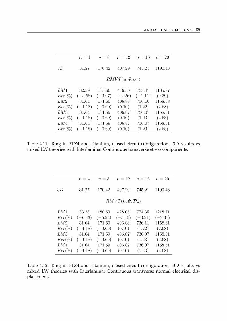
ANALYTICAL SOLUTIONS 85
n = 4 n = 8 n = 12 n = 16 n = 20
3D 31.27 170.42 407.29 745.21 1190.48
RMV T (u, Φ, σn)
LM1 32.39 175.66 416.50 753.47 1185.87Err(%) (−3.58) (−3.07) (−2.26) (−1.11) (0.39)LM2 31.64 171.60 406.88 736.10 1158.58Err(%) (−1.18) (−0.69) (0.10) (1.22) (2.68)LM3 31.64 171.59 406.87 736.07 1158.51Err(%) (−1.18) (−0.69) (0.10) (1.23) (2.68)LM4 31.64 171.59 406.87 736.07 1158.51Err(%) (−1.18) (−0.69) (0.10) (1.23) (2.68)
Table 4.11: Ring in PTZ4 and Titanium, closed circuit configuration. 3D results vsmixed LW theories with Interlaminar Continuous transverse stress components.
n = 4 n = 8 n = 12 n = 16 n = 20
3D 31.27 170.42 407.29 745.21 1190.48
RMV T (u, Φ, Dn)
LM1 33.28 180.53 428.05 774.35 1218.71Err(%) (−6.43) (−5.93) (−5.10) (−3.91) (−2.37)LM2 31.64 171.60 406.88 736.11 1158.61Err(%) (−1.18) (−0.69) (0.10) (1.22) (2.68)LM3 31.64 171.59 406.87 736.07 1158.51Err(%) (−1.18) (−0.69) (0.10) (1.23) (2.68)LM4 31.64 171.59 406.87 736.07 1158.51Err(%) (−1.18) (−0.69) (0.10) (1.23) (2.68)
Table 4.12: Ring in PTZ4 and Titanium, closed circuit configuration. 3D results vsmixed LW theories with Interlaminar Continuous transverse normal electrical dis-placement.
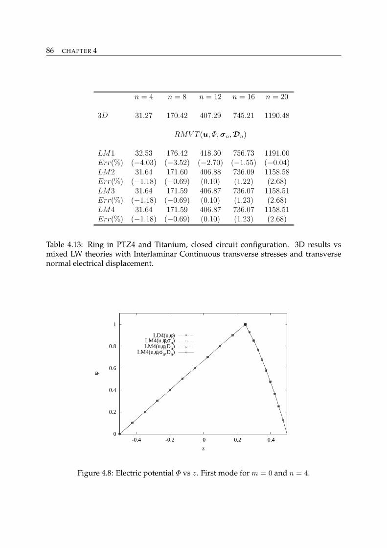
86 CHAPTER 4
n = 4 n = 8 n = 12 n = 16 n = 20
3D 31.27 170.42 407.29 745.21 1190.48
RMV T (u, Φ, σn,Dn)
LM1 32.53 176.42 418.30 756.73 1191.00Err(%) (−4.03) (−3.52) (−2.70) (−1.55) (−0.04)LM2 31.64 171.60 406.88 736.09 1158.58Err(%) (−1.18) (−0.69) (0.10) (1.22) (2.68)LM3 31.64 171.59 406.87 736.07 1158.51Err(%) (−1.18) (−0.69) (0.10) (1.23) (2.68)LM4 31.64 171.59 406.87 736.07 1158.51Err(%) (−1.18) (−0.69) (0.10) (1.23) (2.68)
Table 4.13: Ring in PTZ4 and Titanium, closed circuit configuration. 3D results vsmixed LW theories with Interlaminar Continuous transverse stresses and transversenormal electrical displacement.
0
0.2
0.4
0.6
0.8
1
-0.4 -0.2 0 0.2 0.4
φ
z
LD4(u,φ)LM4(u,φ,σn)LM4(u,φ,Dn)
LM4(u,φ,σn,Dn)
Figure 4.8: Electric potential Φ vs z. First mode for m = 0 and n = 4.
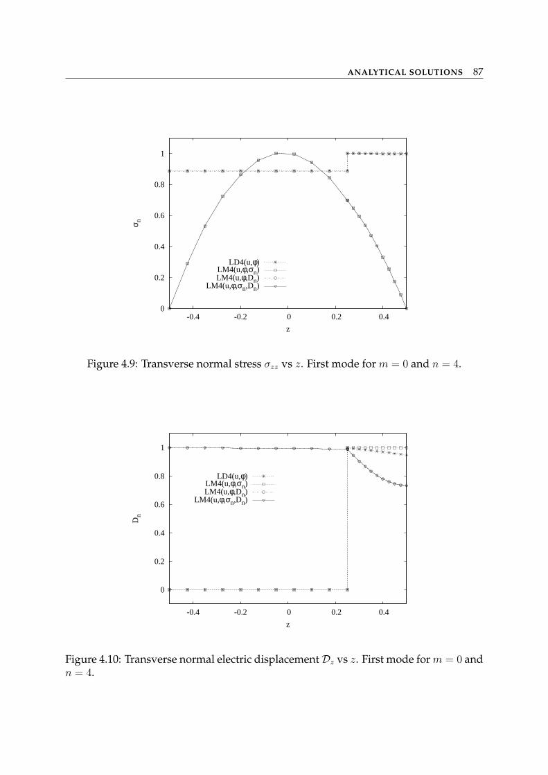
ANALYTICAL SOLUTIONS 87
0
0.2
0.4
0.6
0.8
1
-0.4 -0.2 0 0.2 0.4
σ n
z
LD4(u,φ)LM4(u,φ,σn)LM4(u,φ,Dn)
LM4(u,φ,σn,Dn)
Figure 4.9: Transverse normal stress σzz vs z. First mode for m = 0 and n = 4.
0
0.2
0.4
0.6
0.8
1
-0.4 -0.2 0 0.2 0.4
Dn
z
LD4(u,φ)LM4(u,φ,σn)LM4(u,φ,Dn)
LM4(u,φ,σn,Dn)
Figure 4.10: Transverse normal electric displacementDz vs z. First mode for m = 0 andn = 4.
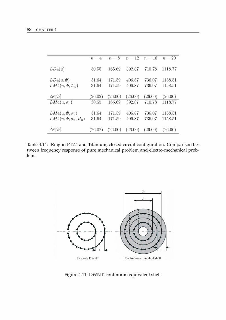
88 CHAPTER 4
n = 4 n = 8 n = 12 n = 16 n = 20
LD4(u) 30.55 165.69 392.87 710.78 1118.77
LD4(u, Φ) 31.64 171.59 406.87 736.07 1158.51LM4(u, Φ,Dn) 31.64 171.59 406.87 736.07 1158.51
∆p[%] (26.02) (26.00) (26.00) (26.00) (26.00)LM4(u, σn) 30.55 165.69 392.87 710.78 1118.77
LM4(u, Φ, σn) 31.64 171.59 406.87 736.07 1158.51LM4(u, Φ, σn,Dn) 31.64 171.59 406.87 736.07 1158.51
∆p[%] (26.02) (26.00) (26.00) (26.00) (26.00)
Table 4.14: Ring in PTZ4 and Titanium, closed circuit configuration. Comparison be-tween frequency response of pure mechanical problem and electro-mechanical prob-lem.
Discrete DWNT Continuum equivalent shell
t t
d1
d2
Figure 4.11: DWNT: continuum equivalent shell.
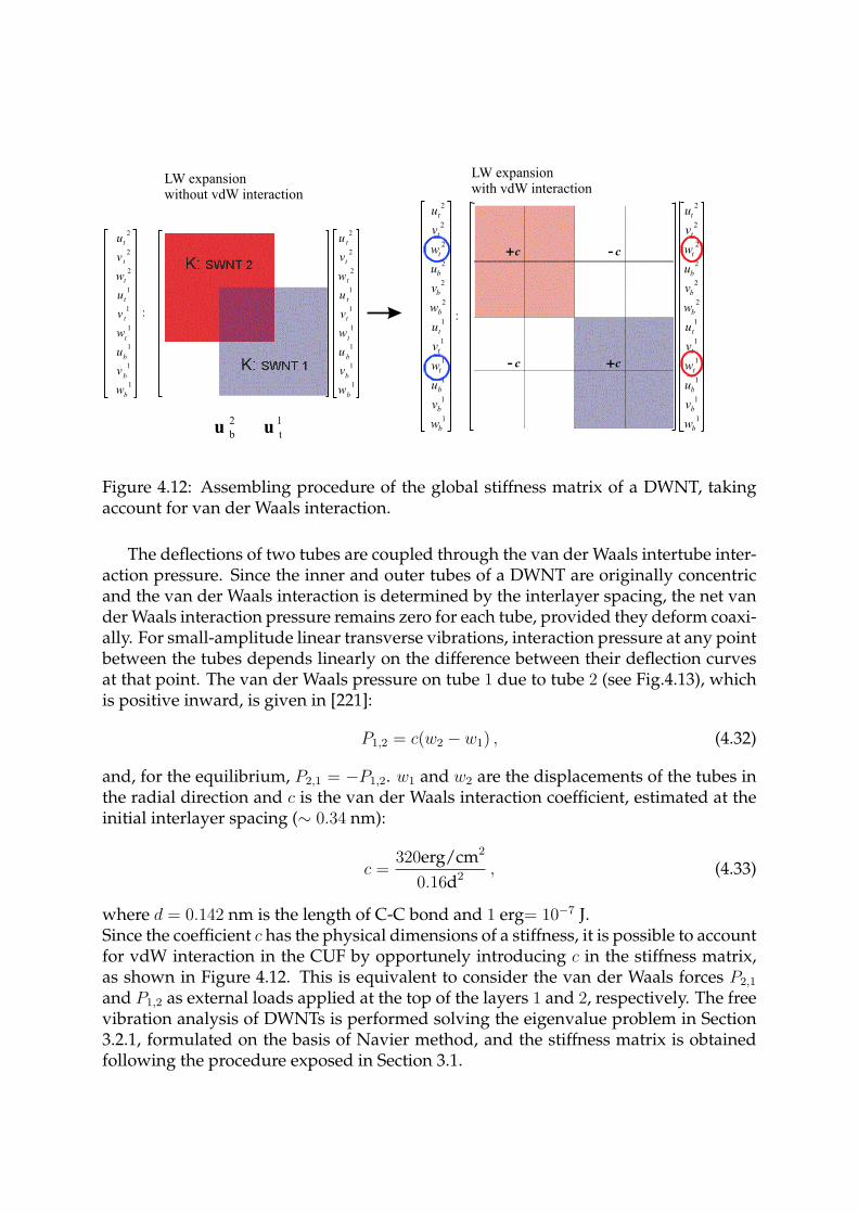
[ ] uM
w
v
u
w
v
u
w
v
u
w
v
u
w
v
u
w
v
u
w
v
u
w
v
u
b
b
b
t
t
t
b
b
b
t
t
t
b
b
b
t
t
t
b
b
b
t
t
t
&&=
ïïïïïïïï
þ
ïïïïïïïï
ý
ü
ïïïïïïïï
î
ïïïïïïïï
í
ì
úúúúúúúúúúúúúúúúú
û
ù
êêêêêêêêêêêêêêêêê
ë
é
ïïïïïïïï
þ
ïïïïïïïï
ý
ü
ïïïïïïïï
î
ïïïïïïïï
í
ì
1
1
1
1
1
1
2
2
2
2
2
2
1
1
1
1
1
1
2
2
2
2
2
2
:
d
d
d
d
d
d
d
d
d
d
d
d
úúúúúúúúúúúúúúúúú
û
ù
êêêêêêêêêêêêêêêêê
ë
é
+-
-+
cc
cc+
+-
-
[ ] uM
w
v
u
w
v
u
w
v
u
w
v
u
w
v
u
w
v
u
b
b
b
t
t
t
t
t
t
b
b
b
t
t
t
t
t
t
&&=
ïïïïïï
þ
ïïïïïï
ý
ü
ïïïïïï
î
ïïïïïï
í
ì
úúúúúúúúúúúú
û
ù
êêêêêêêêêêêê
ë
é
ïïïïïï
þ
ïïïïïï
ý
ü
ïïïïïï
î
ïïïïïï
í
ì
1
1
1
1
1
1
2
2
2
1
1
1
1
1
1
2
2
2
:
d
d
d
d
d
d
d
d
d
1
t
2
buu =
LW expansionwithout vdW interaction
LW expansionwith vdW interaction
Figure 4.12: Assembling procedure of the global stiffness matrix of a DWNT, takingaccount for van der Waals interaction.
The deflections of two tubes are coupled through the van der Waals intertube inter-action pressure. Since the inner and outer tubes of a DWNT are originally concentricand the van der Waals interaction is determined by the interlayer spacing, the net vander Waals interaction pressure remains zero for each tube, provided they deform coaxi-ally. For small-amplitude linear transverse vibrations, interaction pressure at any pointbetween the tubes depends linearly on the difference between their deflection curvesat that point. The van der Waals pressure on tube 1 due to tube 2 (see Fig.4.13), whichis positive inward, is given in [221]:
P1,2 = c(w2 − w1) , (4.32)
and, for the equilibrium, P2,1 = −P1,2. w1 and w2 are the displacements of the tubes inthe radial direction and c is the van der Waals interaction coefficient, estimated at theinitial interlayer spacing (∼ 0.34 nm):
c =320erg/cm2
0.16d2 , (4.33)
where d = 0.142 nm is the length of C-C bond and 1 erg= 10−7 J.Since the coefficient c has the physical dimensions of a stiffness, it is possible to accountfor vdW interaction in the CUF by opportunely introducing c in the stiffness matrix,as shown in Figure 4.12. This is equivalent to consider the van der Waals forces P2,1
and P1,2 as external loads applied at the top of the layers 1 and 2, respectively. The freevibration analysis of DWNTs is performed solving the eigenvalue problem in Section3.2.1, formulated on the basis of Navier method, and the stiffness matrix is obtainedfollowing the procedure exposed in Section 3.1.
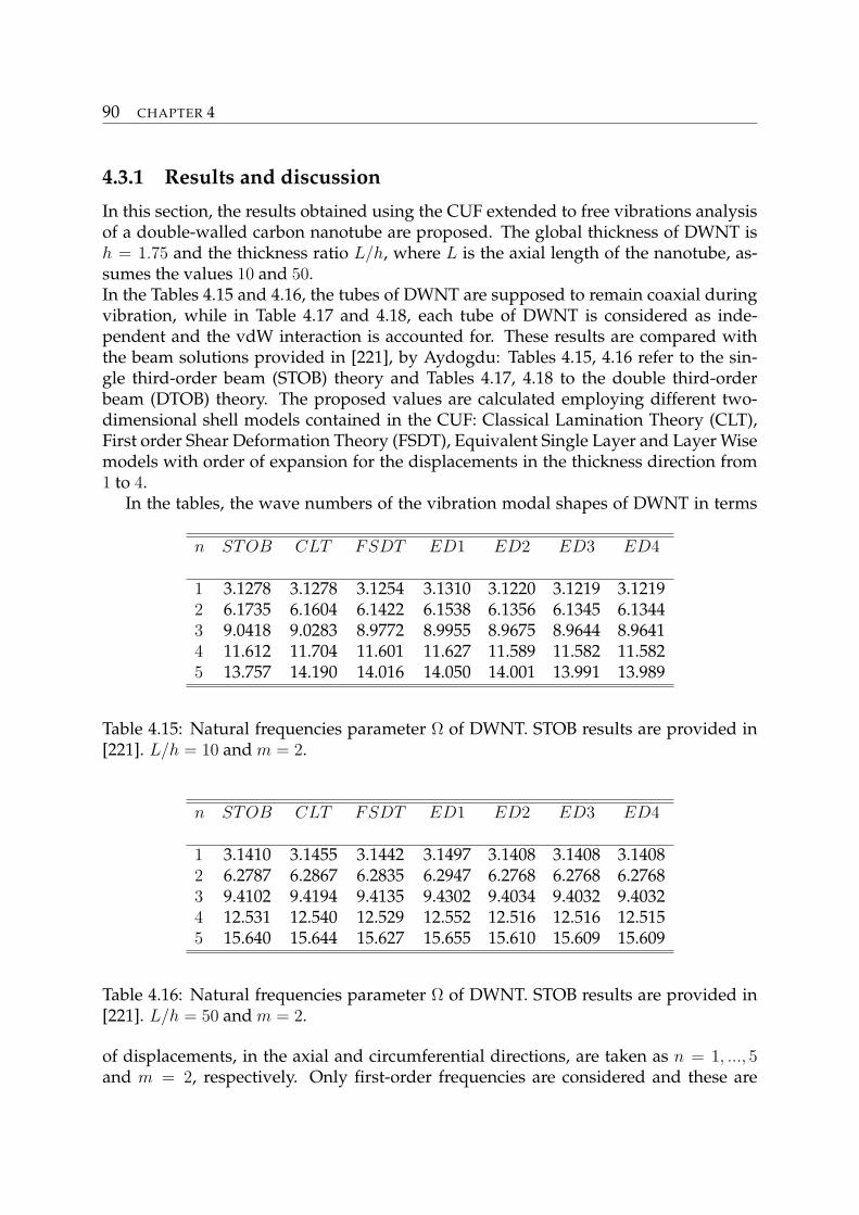
90 CHAPTER 4
4.3.1 Results and discussion
In this section, the results obtained using the CUF extended to free vibrations analysisof a double-walled carbon nanotube are proposed. The global thickness of DWNT ish = 1.75 and the thickness ratio L/h, where L is the axial length of the nanotube, as-sumes the values 10 and 50.In the Tables 4.15 and 4.16, the tubes of DWNT are supposed to remain coaxial duringvibration, while in Table 4.17 and 4.18, each tube of DWNT is considered as inde-pendent and the vdW interaction is accounted for. These results are compared withthe beam solutions provided in [221], by Aydogdu: Tables 4.15, 4.16 refer to the sin-gle third-order beam (STOB) theory and Tables 4.17, 4.18 to the double third-orderbeam (DTOB) theory. The proposed values are calculated employing different two-dimensional shell models contained in the CUF: Classical Lamination Theory (CLT),First order Shear Deformation Theory (FSDT), Equivalent Single Layer and Layer Wisemodels with order of expansion for the displacements in the thickness direction from1 to 4.
In the tables, the wave numbers of the vibration modal shapes of DWNT in terms
n STOB CLT FSDT ED1 ED2 ED3 ED4
1 3.1278 3.1278 3.1254 3.1310 3.1220 3.1219 3.12192 6.1735 6.1604 6.1422 6.1538 6.1356 6.1345 6.13443 9.0418 9.0283 8.9772 8.9955 8.9675 8.9644 8.96414 11.612 11.704 11.601 11.627 11.589 11.582 11.5825 13.757 14.190 14.016 14.050 14.001 13.991 13.989
Table 4.15: Natural frequencies parameter Ω of DWNT. STOB results are provided in[221]. L/h = 10 and m = 2.
n STOB CLT FSDT ED1 ED2 ED3 ED4
1 3.1410 3.1455 3.1442 3.1497 3.1408 3.1408 3.14082 6.2787 6.2867 6.2835 6.2947 6.2768 6.2768 6.27683 9.4102 9.4194 9.4135 9.4302 9.4034 9.4032 9.40324 12.531 12.540 12.529 12.552 12.516 12.516 12.5155 15.640 15.644 15.627 15.655 15.610 15.609 15.609
Table 4.16: Natural frequencies parameter Ω of DWNT. STOB results are provided in[221]. L/h = 50 and m = 2.
of displacements, in the axial and circumferential directions, are taken as n = 1, ..., 5and m = 2, respectively. Only first-order frequencies are considered and these are
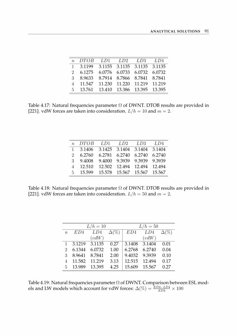
ANALYTICAL SOLUTIONS 91
n DTOB LD1 LD2 LD3 LD41 3.1199 3.1155 3.1135 3.1135 3.11352 6.1275 6.0776 6.0733 6.0732 6.07323 8.9633 8.7914 8.7866 8.7841 8.78414 11.547 11.230 11.220 11.219 11.2195 13.761 13.410 13.386 13.395 13.395
Table 4.17: Natural frequencies parameter Ω of DWNT. DTOB results are provided in[221]. vdW forces are taken into consideration. L/h = 10 and m = 2.
n DTOB LD1 LD2 LD3 LD41 3.1406 3.1425 3.1404 3.1404 3.14042 6.2760 6.2781 6.2740 6.2740 6.27403 9.4008 9.4000 9.3939 9.3939 9.39394 12.510 12.502 12.494 12.494 12.4945 15.599 15.578 15.567 15.567 15.567
Table 4.18: Natural frequencies parameter Ω of DWNT. DTOB results are provided in[221]. vdW forces are taken into consideration. L/h = 50 and m = 2.
L/h = 10 L/h = 50n ED4 LD4 ∆(%) ED4 LD4 ∆(%)
(vdW ) (vdW )1 3.1219 3.1135 0.27 3.1408 3.1404 0.012 6.1344 6.0732 1.00 6.2768 6.2740 0.043 8.9641 8.7841 2.00 9.4032 9.3939 0.104 11.582 11.219 3.13 12.515 12.494 0.175 13.989 13.395 4.25 15.609 15.567 0.27
Table 4.19: Natural frequencies parameter Ω of DWNT. Comparison between ESL mod-els and LW models which account for vdW forces: ∆(%) = ED4−LD4
ED4× 100
92 CHAPTER 4
normalized according to the formula:
Ω =4
√ρAω2L4
EI, (4.34)
where A and I are the area and moment of inertia of the DWNT cross section.Tables 4.15-4.18 show that the CUF results are in good agreement with the referencesolution by increasing the order of expansion of the theory. It should be consideredthat shell models are compared with beam models, therefore some differences betweenthem remain even though high orders of expansion (N = 4) are used. However, thesedifferences become smaller when the nanotube is longer (L/h = 50), because the beamhypotheses are fulfilled, and lower frequencies are considered (low n). In particular,looking at the Tables 4.15 and 4.16 it is possible to note that in general CLT and FSDTtheories give results that are further from the reference solution, compared with theESL models. In some cases, such as in Table 4.16 for n = 4 and n = 5, CLT and FSDTtheories give a smaller error in respect to high-order equivalent single layer theories,but this inconsistency is due to the error that a beam model, as is the STOB, produceson high frequencies. ED4 and LD4 models are compared in Table 4.19. The percentagedifference ∆(%) = ED4−LD4
ED4×100 between them increases for short DWNTs and higher
frequencies, therefore it is possible to conclude that in these cases it is necessary to con-sider the vdW interaction between the DWNT tubes in order to avoid overestimatedresults.For more details about the free vibration analysis of DWNTs, one can refer to [222].
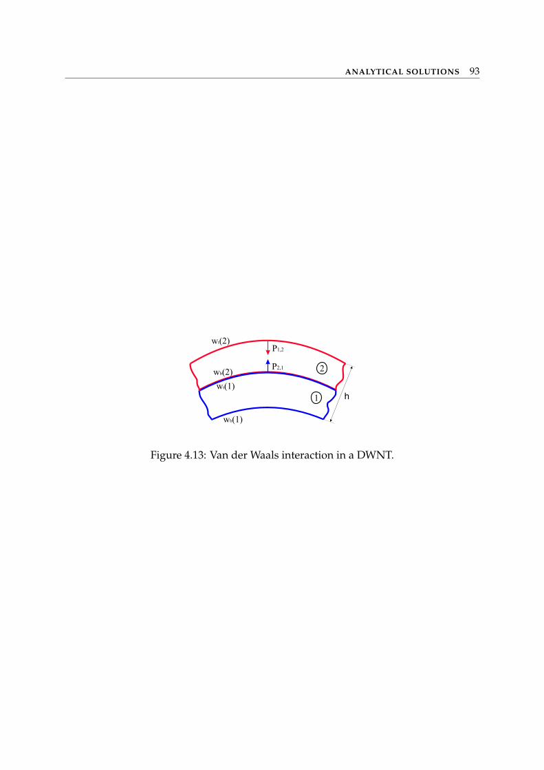
ANALYTICAL SOLUTIONS 93
wt(2)
wb(2)
wt(1)
wb(1)
1
2
h
P1,2
P2,1
Figure 4.13: Van der Waals interaction in a DWNT.

Chapter 5
FEM solutions
The FEM model here presented for the analysis of shells does not involve any approximation ofthe geometry and it is able to accurately describe the curvature of cylindrical shells. Note that,in this chapter, the notation presented in Section 2.2.1 for cylindrical geometry is used. Such amodel is combined with a simple displacement formulation and the MITC method is employedto overcome the membrane and shear locking phenomenon.Firstly, the derivation of the governing equations in the framework of FEM is presented. Then,an assessment of the CUF MITC9 shell element is performed. Some discriminating problemsfrom the literature are considered and the efficiency and the robustness of the shell element aretested. Finally, the results obtained from the analysis of composite and FGM shells are provided.In this case, the superiority of the models contained in the CUF in respect to the classical finiteelements based on the FSDT is demonstrated. For these reasons, it seems reasonable to extendin future the CUF shell element to the analysis of multi-field problems, as made in Chapter 4.
5.1 Governing equations
The governing equations for the static analysis of cylindrical shells subjected to puremechenical loads are derived from the PVD, written in the following form:
∫
Ω
∫
A
δεp
T σp + δεnT σn
H dΩdξ3 =
∫
Ω
∫
A
δupH dΩdξ3 (5.1)
where p = p(ξ1, ξ2, ξ3) is the load applied to the structure.Exploiting the geometrical relations (Eqs.(3.31)) and the constitutive equations (Eqs.(3.33)),in which the FEM approximation and the MITC method have been applied, the PVD
95
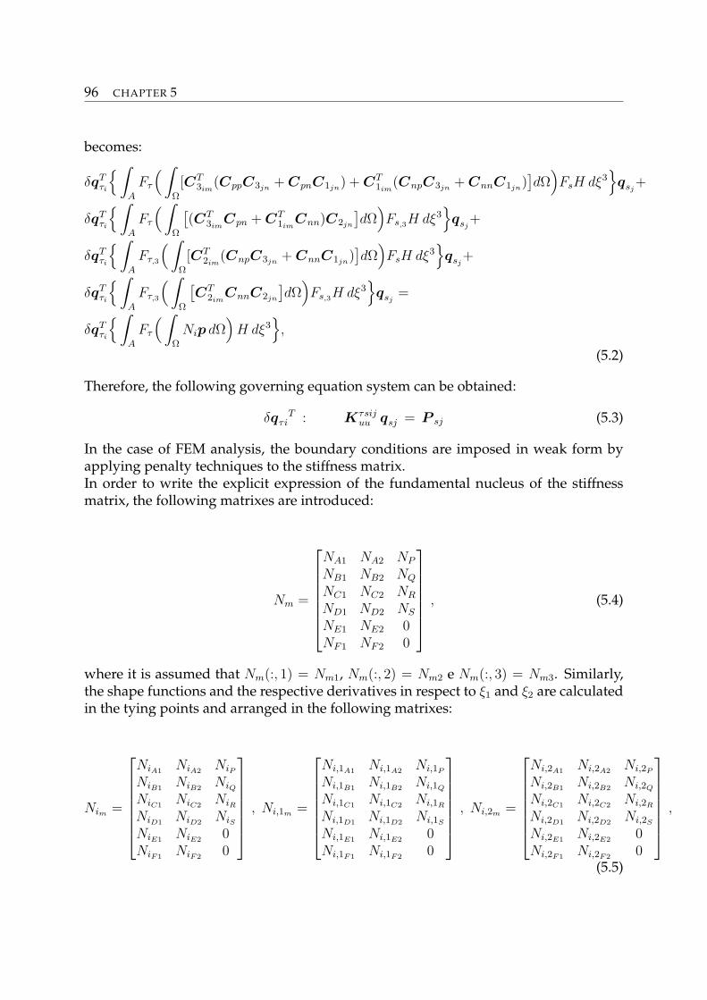
96 CHAPTER 5
becomes:
δqTτi
∫
A
Fτ
( ∫
Ω
[CT3im
(CppC3jn+ CpnC1jn
) + CT1im
(CnpC3jn+ CnnC1jn
)]dΩ
)FsH dξ3
qsj
+
δqTτi
∫
A
Fτ
( ∫
Ω
[(CT
3imCpn + CT
1imCnn)C2jn
]dΩ
)Fs,3H dξ3
qsj
+
δqTτi
∫
A
Fτ,3
( ∫
Ω
[CT2im
(CnpC3jn+ CnnC1jn
)]dΩ
)FsH dξ3
qsj
+
δqTτi
∫
A
Fτ,3
( ∫
Ω
[CT
2imCnnC2jn
]dΩ
)Fs,3H dξ3
qsj
=
δqTτi
∫
A
Fτ
( ∫
Ω
Nip dΩ)
H dξ3
,
(5.2)
Therefore, the following governing equation system can be obtained:
δqτiT : Kτsij
uu qsj = P sj (5.3)
In the case of FEM analysis, the boundary conditions are imposed in weak form byapplying penalty techniques to the stiffness matrix.In order to write the explicit expression of the fundamental nucleus of the stiffnessmatrix, the following matrixes are introduced:
Nm =
NA1 NA2 NP
NB1 NB2 NQ
NC1 NC2 NR
ND1 ND2 NS
NE1 NE2 0NF1 NF2 0
, (5.4)
where it is assumed that Nm(:, 1) = Nm1, Nm(:, 2) = Nm2 e Nm(:, 3) = Nm3. Similarly,the shape functions and the respective derivatives in respect to ξ1 and ξ2 are calculatedin the tying points and arranged in the following matrixes:
Nim =
NiA1NiA2
NiP
NiB1NiB2
NiQ
NiC1NiC2
NiR
NiD1NiD2
NiS
NiE1NiE2
0NiF1
NiF20
, Ni,1m =
Ni,1A1Ni,1A2
Ni,1P
Ni,1B1Ni,1B2
Ni,1Q
Ni,1C1Ni,1C2
Ni,1R
Ni,1D1Ni,1D2
Ni,1S
Ni,1E1Ni,1E2
0Ni,1F1
Ni,1F20
, Ni,2m =
Ni,2A1Ni,2A2
Ni,2P
Ni,2B1Ni,2B2
Ni,2Q
Ni,2C1Ni,2C2
Ni,2R
Ni,2D1Ni,2D2
Ni,2S
Ni,2E1Ni,2E2
0Ni,2F1
Ni,2F20
,
(5.5)
FEM SOLUTIONS 97
and it is assumed that:
Nim(:, 1) = Nim1 , Nim(:, 2) = Nim2 , Nim(:, 3) = Nim3
Ni,1m(:, 1) = Ni,1m1 , Ni,1m(:, 2) = Ni,1m2 , Ni,1m(:, 3) = Ni,1m3
Ni,2m(:, 1) = Ni,2m1 , Ni,2m(:, 2) = Ni,2m2 , Ni,2m(:, 3) = Ni,2m3
(5.6)
Therefore the components of the fundamental nucleus Kτsijuu are:
Kτsijmn11 =Ck
55Nim1 C Nm1Nn1 BΩ Njn1 C HFτ,3Fs,3 BA +
C11Ni,1m1 C Nm1Nn1 BΩ Nj,1n1 C HFτFs BA +
C16Ni,2m3 C Nm3Nn1 BΩ Nj,1n1 C HFτFs BA +
C16Ni,1m1 C Nm1Nn3 BΩ Nj,2n3 C HFτFs BA +
C66Ni,2m3 C Nm3Nn3 BΩ Nj,2n3 C HFτFsBA
Kτsijmn12 =− Ck
45
1
RNim1 C Nm1Nn2 BΩ Njn2 C HFτ,3Fs BA +
C45Nim1 C Nm1Nn2 BΩ Njn2 C H2Fτ,3Fs,3 BA +
C12Ni,1m1 C Nm1Nn2 BΩ Nj,2n2 C H2FτFs BA +
C16Ni,1m1 C Nm1Nn3 BΩ Nj,1n3 C H2FτFs BA +
C26Ni,2m3 C Nm3Nn2 BΩ Nj,2n2 C H2FτFs BA +
C66Ni,2m3 C Nm3Nn3 BΩ Nj,1n3 C H2FτFsBA
Kτsijmn13 =Ck
13Ni,1m1 C Nm1Nj BΩ CHFτFs,3 BA +
C36Ni,2m3 C Nm3Nj BΩ CHFτFs,3 BA +
C121
RNi,1m1 C Nm1Nn2 BΩ Njn2 C H2FτFs BA +
C261
RNi,2m3 C Nm3Nn2 BΩ Njn2 C H2FτFs BA +
C55Nim1 C Nm1Nn1 BΩ Nj,1n1 C HFτ,3Fs BA +
C45Nim1 C Nm1Nn2 BΩ Nj,2n2 C HFτ,3FsBA
(5.7)
98 CHAPTER 5
Kτsijmn21 =− Ck
45
1
RNim2 C Nm2Nn1 BΩ Njn1 C HFτFs,3 BA +
C45Nim2 C Nm2Nn1 BΩ Njn1 C H2Fτ,3Fs,3 BA +
C12Ni,2m2 C Nm2Nn1 BΩ Nj,1n1 C H2FτFs BA +
C16Ni,1m3 C Nm3Nn1 BΩ Nj,1n1 C H2FτFs BA +
C26Ni,2m2 C Nm2Nn3 BΩ Nj,2n3 C H2FτFs BA +
C66Ni,1m3 C Nm3Nn3 BΩ Nj,2n3 C H2FτFsBA
Kτsijmn22 =Ck
22Ni,2m2 C Nm2Nn2 BΩ Nj,2n2 C H3FτFs BA +
C26Ni,2m2 C Nm2Nn3 BΩ Nj,1n3 C H3FτFsBA
C26Ni,1m3 C Nm3Nn2 BΩ Nj,2n2 C H3FτFs BA +
C66Ni,1m3 C Nm3Nn3 BΩ Nj,1n3 C H3FτFs BA +
C441
R2Nim2 C Nm2Nn2 BΩ Njn2 C HFτFs BA −
C441
RNim2 C Nm2Nn2 BΩ Njn2 C H2FτFs,3 BA −
C441
RNim2 C Nm2Nn2 BΩ Njn2 C H2Fτ,3Fs BA +
C44Nim2 C Nm2Nn2 BΩ Njn2 C H3Fτ,3Fs,3BA
Kτsijmn23 =Ck
22
1
RNi,2m2 C Nm2Nn2 BΩ Njn2 C H3FτFs BA +
C23Ni,2m2 C Nm2Nj BΩ CH2FτFs,3 BA +
C261
RNi,1m3 C Nm3Nn2 BΩ Njn2 C H3FτFs BA +
C36Ni,1m3 C Nm3Nj BΩ CH2FτFs,3 BA −C45
1
RNim2 C Nm2Nn1 BΩ Nj,1n1 C HFτFs BA −
C441
RNim2 C Nm2Nn2 BΩ Nj,2n2 C HFτFs BA +
C45Nim2 C Nm2Nn1 BΩ Nj,1n1 C H2Fτ,3Fs BA +
C44Nim2 C Nm2Nn2 BΩ Nj,2n2 C H2Fτ,3FsBA
(5.8)
FEM SOLUTIONS 99
Kτsijmn31 =Ck
55Ni,1m1 C Nm1Nn1 BΩ Njn1 C HFτFs,3 BA +
C45Ni,2m2 C Nm2Nn1 BΩ Njn1 C HFτFs,3 BA +
C121
RNim2 C Nm2Nn1 BΩ Nj,1n1 C H2FτFs BA +
C13 C NiNn1 BΩ Nj,1n1 C HFτ,3Fs BA +
C261
RNim2 C Nm2Nn3 BΩ Nj,2n3 C H2FτFs BA +
C36 C NiNn3 BΩ Nj,2n3 C HFτ,3FsBA
Kτsijmn32 =Ck
22
1
RNim2 C Nm2Nn2 BΩ Nj,2n2 C H3FτFs BA +
C23 C NiNn2 BΩ Nj,2n2 C H2Fτ,3Fs BA +
C261
RNim2 C Nm2Nn3 BΩ Nj,1n3 C H3FτFs BA +
C36 C NiNn3 BΩ Nj,1n3 C H2Fτ,3Fs BA −C45
1
RNi,1m1 C Nm1Nn2 BΩ Njn2 C HFτFs BA −
C441
RNi,2m2 C Nm2Nn2 BΩ Njn2 C HFτFs BA +
C45Ni,1m1 C Nm1Nn2 BΩ Njn2 C H2FτFs,3 BA +
C44Ni,2m2 C Nm2Nn2 BΩ Njn2 C H2FτFsBA
Kτsijmn33 =Ck
22
1
R2Nim2 C Nm2Nn2 BΩ Njn2 C H3FτFs BA +
C231
RNim2 C Nm2Nj BΩ CH2FτFs,3 BA +
C231
RC NiNn2 BΩ Njn2 C H2Fτ,3Fs BA +
C33 C NiNj BΩ CHFτ,3Fs,3 BA +
C55Ni,1m1 C Nm1Nn1 BΩ Nj,1n1 C HFτFs BA +
C45Ni,2m2 C Nm2Nn1 BΩ Nj,1n1 C HFτFs BA +
C45Ni,1m1 C Nm1Nn2 BΩ Nj,2n2 C HFτFs BA +
C44Ni,2m2 C Nm2Nn2 BΩ Nj,2n2 C HFτFsBA
(5.9)
where:C(. . .)BΩ =
∫
Ω
(. . .)dΩ , C(. . .)BA =
∫
A
(. . .)dξ3 (5.10)
The fundamental nucleus is expanded on the sum indexes m,n = 1, ..., 6 (that is a loopon the tying points), i, j = 1, ..., 9 and τ, s = 0, ..., N in order to build the stiffnessmatrix of each element. Then, the stiffness matrixes are assembled at element level
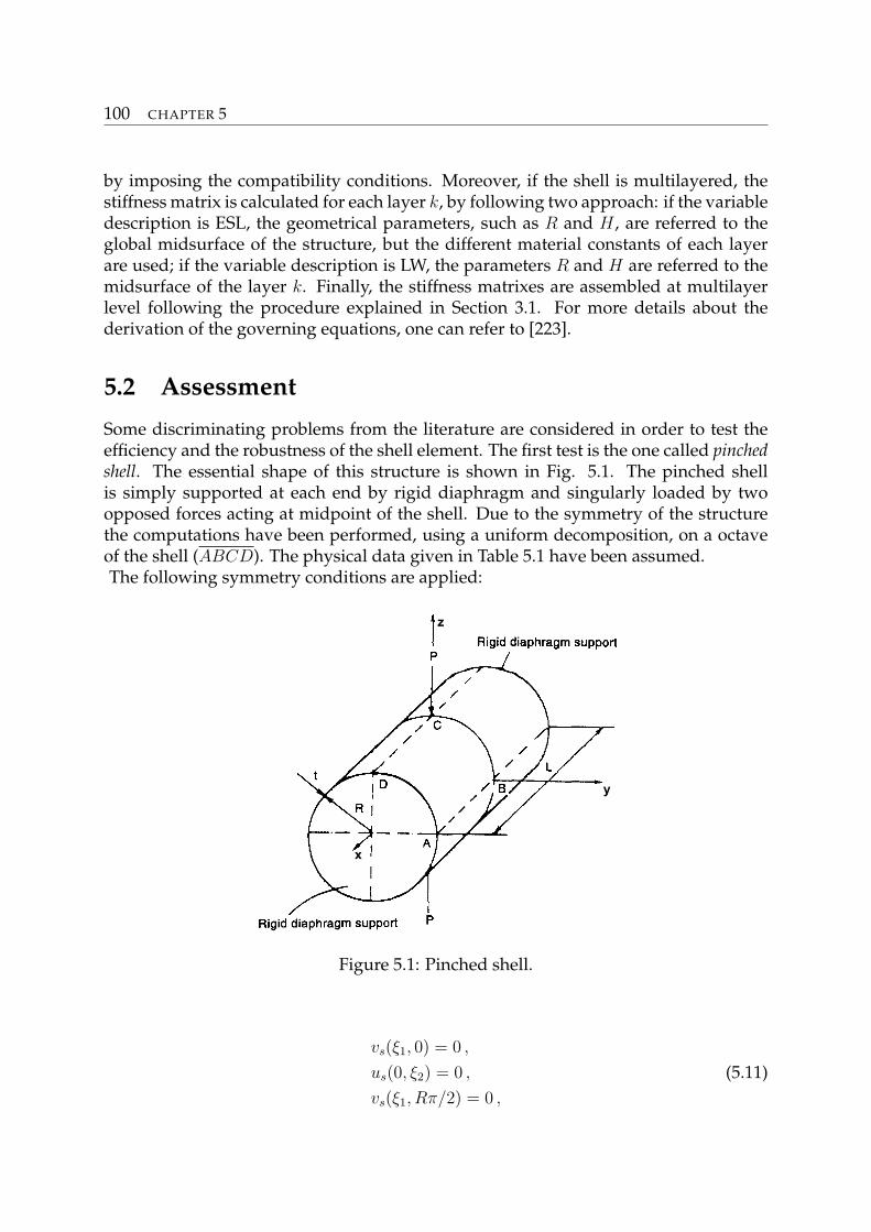
100 CHAPTER 5
by imposing the compatibility conditions. Moreover, if the shell is multilayered, thestiffness matrix is calculated for each layer k, by following two approach: if the variabledescription is ESL, the geometrical parameters, such as R and H , are referred to theglobal midsurface of the structure, but the different material constants of each layerare used; if the variable description is LW, the parameters R and H are referred to themidsurface of the layer k. Finally, the stiffness matrixes are assembled at multilayerlevel following the procedure explained in Section 3.1. For more details about thederivation of the governing equations, one can refer to [223].
5.2 Assessment
Some discriminating problems from the literature are considered in order to test theefficiency and the robustness of the shell element. The first test is the one called pinchedshell. The essential shape of this structure is shown in Fig. 5.1. The pinched shellis simply supported at each end by rigid diaphragm and singularly loaded by twoopposed forces acting at midpoint of the shell. Due to the symmetry of the structurethe computations have been performed, using a uniform decomposition, on a octaveof the shell (ABCD). The physical data given in Table 5.1 have been assumed.The following symmetry conditions are applied:
x
y
z
Figure 5.1: Pinched shell.
vs(ξ1, 0) = 0 ,
us(0, ξ2) = 0 ,
vs(ξ1, Rπ/2) = 0 ,
(5.11)
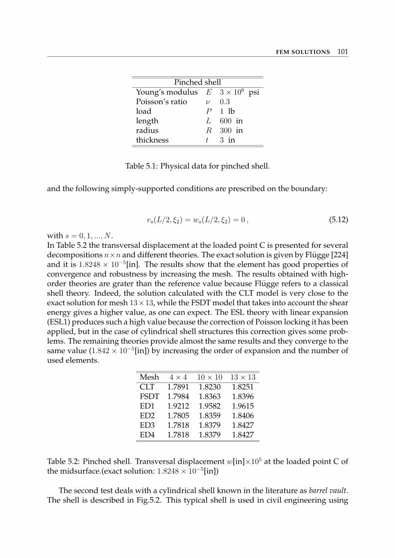
FEM SOLUTIONS 101
Pinched shellYoung’s modulus E 3× 10⁶ psiPoisson’s ratio ν 0.3load P 1 lblength L 600 inradius R 300 inthickness t 3 in
Table 5.1: Physical data for pinched shell.
and the following simply-supported conditions are prescribed on the boundary:
vs(L/2, ξ2) = ws(L/2, ξ2) = 0 , (5.12)
with s = 0, 1, ..., N .In Table 5.2 the transversal displacement at the loaded point C is presented for severaldecompositions n×n and different theories. The exact solution is given by Flugge [224]and it is 1.8248 × 10⁻⁵[in]. The results show that the element has good properties ofconvergence and robustness by increasing the mesh. The results obtained with high-order theories are grater than the reference value because Flugge refers to a classicalshell theory. Indeed, the solution calculated with the CLT model is very close to theexact solution for mesh 13×13, while the FSDT model that takes into account the shearenergy gives a higher value, as one can expect. The ESL theory with linear expansion(ESL1) produces such a high value because the correction of Poisson locking it has beenapplied, but in the case of cylindrical shell structures this correction gives some prob-lems. The remaining theories provide almost the same results and they converge to thesame value (1.842 × 10⁻⁵[in]) by increasing the order of expansion and the number ofused elements.
Mesh 4× 4 10× 10 13× 13CLT 1.7891 1.8230 1.8251FSDT 1.7984 1.8363 1.8396ED1 1.9212 1.9582 1.9615ED2 1.7805 1.8359 1.8406ED3 1.7818 1.8379 1.8427ED4 1.7818 1.8379 1.8427
Table 5.2: Pinched shell. Transversal displacement w[in]×105 at the loaded point C ofthe midsurface.(exact solution: 1.8248× 10⁻⁵[in])
The second test deals with a cylindrical shell known in the literature as barrel vault.The shell is described in Fig.5.2. This typical shell is used in civil engineering using
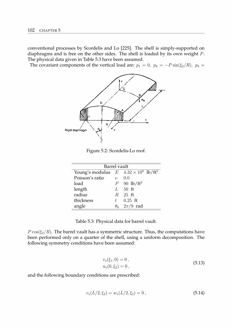
102 CHAPTER 5
conventional processes by Scordelis and Lo [225]. The shell is simply-supported ondiaphragms and is free on the other sides. The shell is loaded by its own weight P .The physical data given in Table 5.3 have been assumed.The covariant components of the vertical load are: p1 = 0, p2 = −P sin(ξ2/R), p3 =
x
y
z
Figure 5.2: Scordelis-Lo roof.
Barrel vaultYoung’s modulus E 4.32× 10⁸ lb/ft2
Poisson’s ratio ν 0.0load P 90 lb/ft2
length L 50 ftradius R 25 ftthickness t 0.25 ftangle θ0 2π/9 rad
Table 5.3: Physical data for barrel vault.
P cos(ξ2/R). The barrel vault has a symmetric structure. Thus, the computations havebeen performed only on a quarter of the shell, using a uniform decomposition. Thefollowing symmetry conditions have been assumed:
vs(ξ1, 0) = 0 ,
us(0, ξ2) = 0 ,(5.13)
and the following boundary conditions are prescribed:
vs(L/2, ξ2) = ws(L/2, ξ2) = 0 , (5.14)
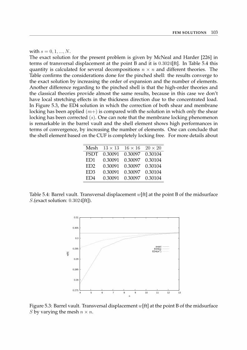
FEM SOLUTIONS 103
with s = 0, 1, ..., N .The exact solution for the present problem is given by McNeal and Harder [226] interms of transversal displacement at the point B and it is 0.3024[ft]. In Table 5.4 thisquantity is calculated for several decompositions n × n and different theories. TheTable confirms the considerations done for the pinched shell: the results converge tothe exact solution by increasing the order of expansion and the number of elements.Another difference regarding to the pinched shell is that the high-order theories andthe classical theories provide almost the same results, because in this case we don’thave local stretching effects in the thickness direction due to the concentrated load.In Figure 5.3, the ED4 solution in which the correction of both shear and membranelocking has been applied (m+) is compared with the solution in which only the shearlocking has been corrected (s). One can note that the membrane locking phenomenonis remarkable in the barrel vault and the shell element shows high performances interms of convergence, by increasing the number of elements. One can conclude thatthe shell element based on the CUF is completely locking free. For more details about
Mesh 13× 13 16× 16 20× 20FSDT 0.30091 0.30097 0.30104ED1 0.30091 0.30097 0.30104ED2 0.30091 0.30097 0.30104ED3 0.30091 0.30097 0.30104ED4 0.30091 0.30097 0.30104
Table 5.4: Barrel vault. Transversal displacement w[ft] at the point B of the midsurfaceS.(exact solution: 0.3024[ft]).
0.275
0.28
0.285
0.29
0.295
0.3
0.305
0.31
4 5 6 7 8 9 10 11 12 13
w[ft
]
n
exactED4(s)
ED4(m+)
Figure 5.3: Barrel vault. Transversal displacement w[ft] at the point B of the midsurfaceS by varying the mesh n× n.
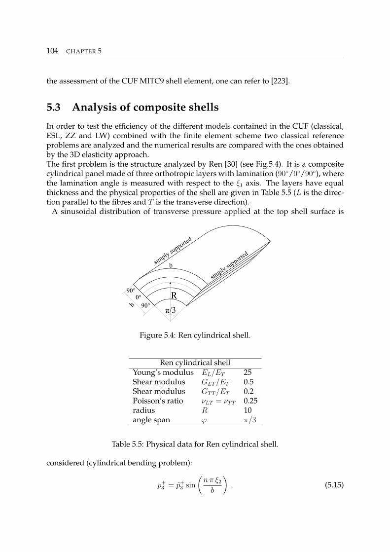
104 CHAPTER 5
the assessment of the CUF MITC9 shell element, one can refer to [223].
5.3 Analysis of composite shells
In order to test the efficiency of the different models contained in the CUF (classical,ESL, ZZ and LW) combined with the finite element scheme two classical referenceproblems are analyzed and the numerical results are compared with the ones obtainedby the 3D elasticity approach.The first problem is the structure analyzed by Ren [30] (see Fig.5.4). It is a compositecylindrical panel made of three orthotropic layers with lamination (90/0/90), wherethe lamination angle is measured with respect to the ξ1 axis. The layers have equalthickness and the physical properties of the shell are given in Table 5.5 (L is the direc-tion parallel to the fibres and T is the transverse direction).
A sinusoidal distribution of transverse pressure applied at the top shell surface is
90°0°
90°
R
π/3
simply su
pported
simply su
pported
b
h
Figure 5.4: Ren cylindrical shell.
Ren cylindrical shellYoung’s modulus EL/ET 25Shear modulus GLT /ET 0.5Shear modulus GTT /ET 0.2Poisson’s ratio νLT = νTT 0.25radius R 10angle span ϕ π/3
Table 5.5: Physical data for Ren cylindrical shell.
considered (cylindrical bending problem):
p+3 = p+
3 sin
(nπ ξ2
b
), (5.15)
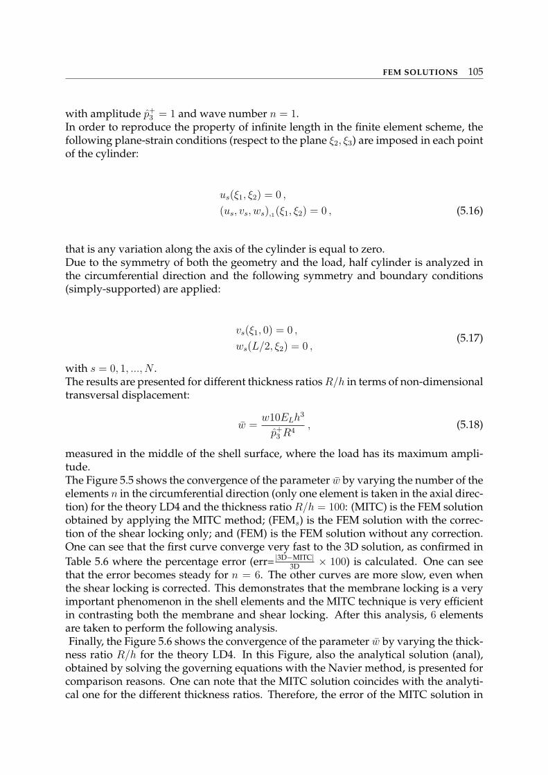
FEM SOLUTIONS 105
with amplitude p+3 = 1 and wave number n = 1.
In order to reproduce the property of infinite length in the finite element scheme, thefollowing plane-strain conditions (respect to the plane ξ2, ξ3) are imposed in each pointof the cylinder:
us(ξ1, ξ2) = 0 ,
(us, vs, ws),1(ξ1, ξ2) = 0 , (5.16)
that is any variation along the axis of the cylinder is equal to zero.Due to the symmetry of both the geometry and the load, half cylinder is analyzed inthe circumferential direction and the following symmetry and boundary conditions(simply-supported) are applied:
vs(ξ1, 0) = 0 ,
ws(L/2, ξ2) = 0 ,(5.17)
with s = 0, 1, ..., N .The results are presented for different thickness ratios R/h in terms of non-dimensionaltransversal displacement:
w =w10ELh3
p+3 R4
, (5.18)
measured in the middle of the shell surface, where the load has its maximum ampli-tude.The Figure 5.5 shows the convergence of the parameter w by varying the number of theelements n in the circumferential direction (only one element is taken in the axial direc-tion) for the theory LD4 and the thickness ratio R/h = 100: (MITC) is the FEM solutionobtained by applying the MITC method; (FEMs) is the FEM solution with the correc-tion of the shear locking only; and (FEM) is the FEM solution without any correction.One can see that the first curve converge very fast to the 3D solution, as confirmed inTable 5.6 where the percentage error (err= |3D−MITC|
3D × 100) is calculated. One can seethat the error becomes steady for n = 6. The other curves are more slow, even whenthe shear locking is corrected. This demonstrates that the membrane locking is a veryimportant phenomenon in the shell elements and the MITC technique is very efficientin contrasting both the membrane and shear locking. After this analysis, 6 elementsare taken to perform the following analysis.Finally, the Figure 5.6 shows the convergence of the parameter w by varying the thick-
ness ratio R/h for the theory LD4. In this Figure, also the analytical solution (anal),obtained by solving the governing equations with the Navier method, is presented forcomparison reasons. One can note that the MITC solution coincides with the analyti-cal one for the different thickness ratios. Therefore, the error of the MITC solution in
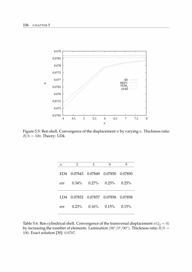
106 CHAPTER 5
0.0745
0.075
0.0755
0.076
0.0765
0.077
0.0775
0.078
0.0785
0.079
4 4.5 5 5.5 6 6.5 7 7.5 8
w
n
3DMITCFEMsFEM
Figure 5.5: Ren shell. Convergence of the displacement w by varying n. Thickness ratioR/h = 100. Theory: LD4.
n 2 4 6 8
ED4 0.07843 0.07849 0.07850 0.07850
err 0.34% 0.27% 0.25% 0.25%
LD4 0.07852 0.07857 0.07858 0.07858
err 0.23% 0.16% 0.15% 0.15%
Table 5.6: Ren cylindrical shell. Convergence of the transversal displacement w(ξ3 = 0)by increasing the number of elements. Lamination (90/0/90). Thickness ratio R/h =100. Exact solution [30]: 0.0787.
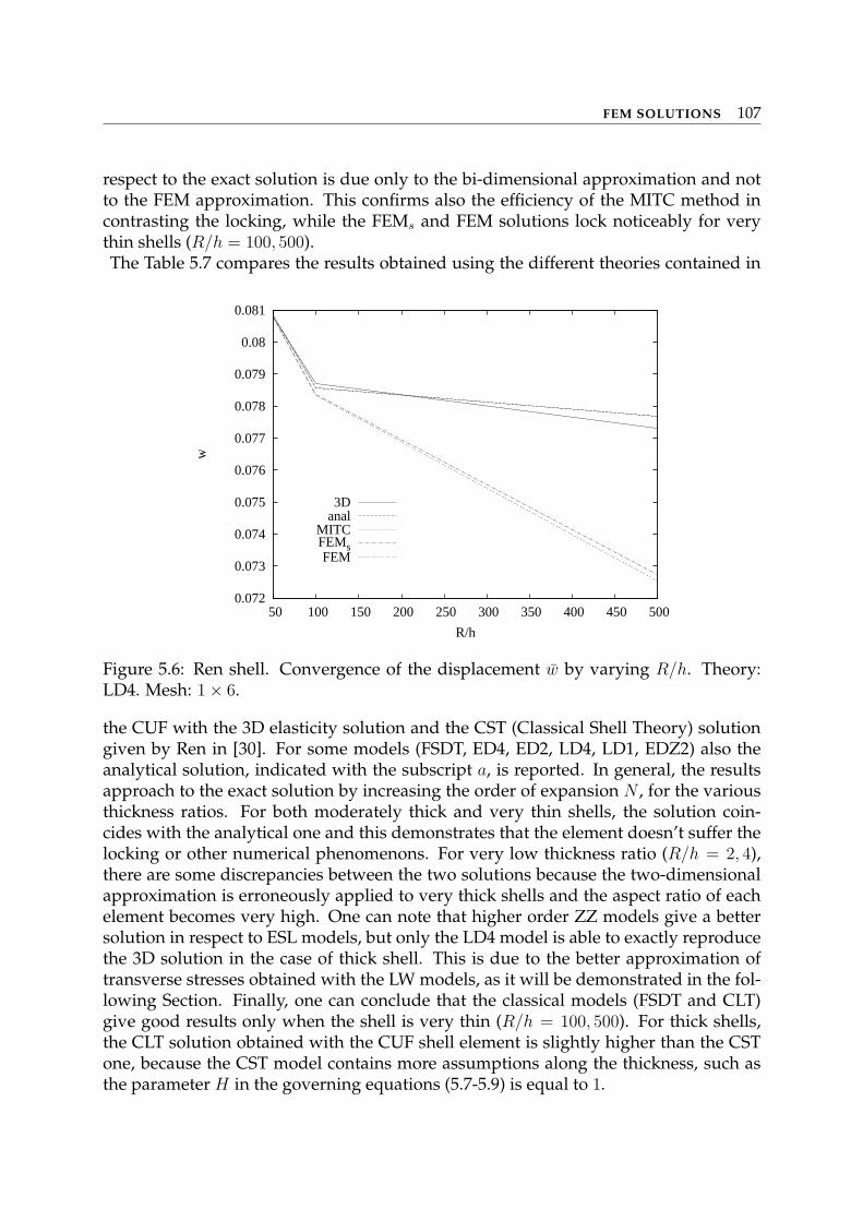
FEM SOLUTIONS 107
respect to the exact solution is due only to the bi-dimensional approximation and notto the FEM approximation. This confirms also the efficiency of the MITC method incontrasting the locking, while the FEMs and FEM solutions lock noticeably for verythin shells (R/h = 100, 500).The Table 5.7 compares the results obtained using the different theories contained in
0.072
0.073
0.074
0.075
0.076
0.077
0.078
0.079
0.08
0.081
50 100 150 200 250 300 350 400 450 500
w
R/h
3Danal
MITCFEMsFEM
Figure 5.6: Ren shell. Convergence of the displacement w by varying R/h. Theory:LD4. Mesh: 1× 6.
the CUF with the 3D elasticity solution and the CST (Classical Shell Theory) solutiongiven by Ren in [30]. For some models (FSDT, ED4, ED2, LD4, LD1, EDZ2) also theanalytical solution, indicated with the subscript a, is reported. In general, the resultsapproach to the exact solution by increasing the order of expansion N , for the variousthickness ratios. For both moderately thick and very thin shells, the solution coin-cides with the analytical one and this demonstrates that the element doesn’t suffer thelocking or other numerical phenomenons. For very low thickness ratio (R/h = 2, 4),there are some discrepancies between the two solutions because the two-dimensionalapproximation is erroneously applied to very thick shells and the aspect ratio of eachelement becomes very high. One can note that higher order ZZ models give a bettersolution in respect to ESL models, but only the LD4 model is able to exactly reproducethe 3D solution in the case of thick shell. This is due to the better approximation oftransverse stresses obtained with the LW models, as it will be demonstrated in the fol-lowing Section. Finally, one can conclude that the classical models (FSDT and CLT)give good results only when the shell is very thin (R/h = 100, 500). For thick shells,the CLT solution obtained with the CUF shell element is slightly higher than the CSTone, because the CST model contains more assumptions along the thickness, such asthe parameter H in the governing equations (5.7-5.9) is equal to 1.
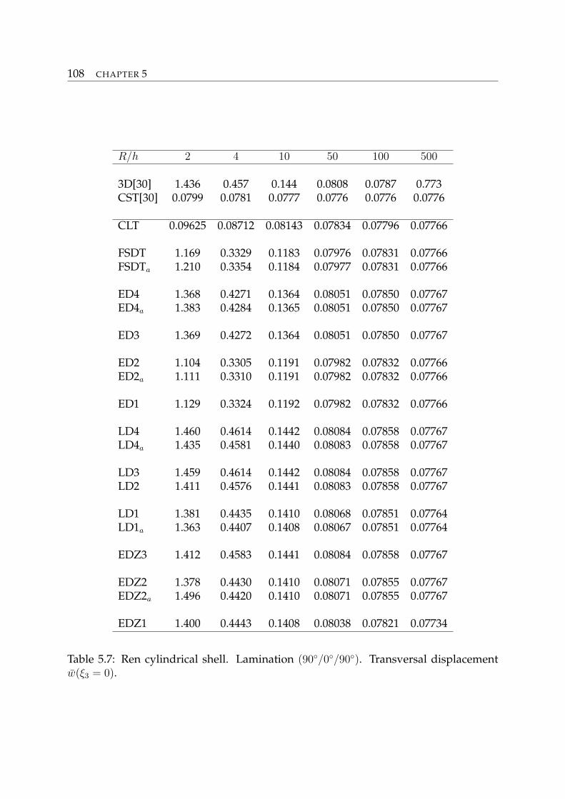
108 CHAPTER 5
R/h 2 4 10 50 100 500
3D[30] 1.436 0.457 0.144 0.0808 0.0787 0.773CST[30] 0.0799 0.0781 0.0777 0.0776 0.0776 0.0776
CLT 0.09625 0.08712 0.08143 0.07834 0.07796 0.07766
FSDT 1.169 0.3329 0.1183 0.07976 0.07831 0.07766FSDTa 1.210 0.3354 0.1184 0.07977 0.07831 0.07766
ED4 1.368 0.4271 0.1364 0.08051 0.07850 0.07767ED4a 1.383 0.4284 0.1365 0.08051 0.07850 0.07767
ED3 1.369 0.4272 0.1364 0.08051 0.07850 0.07767
ED2 1.104 0.3305 0.1191 0.07982 0.07832 0.07766ED2a 1.111 0.3310 0.1191 0.07982 0.07832 0.07766
ED1 1.129 0.3324 0.1192 0.07982 0.07832 0.07766
LD4 1.460 0.4614 0.1442 0.08084 0.07858 0.07767LD4a 1.435 0.4581 0.1440 0.08083 0.07858 0.07767
LD3 1.459 0.4614 0.1442 0.08084 0.07858 0.07767LD2 1.411 0.4576 0.1441 0.08083 0.07858 0.07767
LD1 1.381 0.4435 0.1410 0.08068 0.07851 0.07764LD1a 1.363 0.4407 0.1408 0.08067 0.07851 0.07764
EDZ3 1.412 0.4583 0.1441 0.08084 0.07858 0.07767
EDZ2 1.378 0.4430 0.1410 0.08071 0.07855 0.07767EDZ2a 1.496 0.4420 0.1410 0.08071 0.07855 0.07767
EDZ1 1.400 0.4443 0.1408 0.08038 0.07821 0.07734
Table 5.7: Ren cylindrical shell. Lamination (90/0/90). Transversal displacementw(ξ3 = 0).
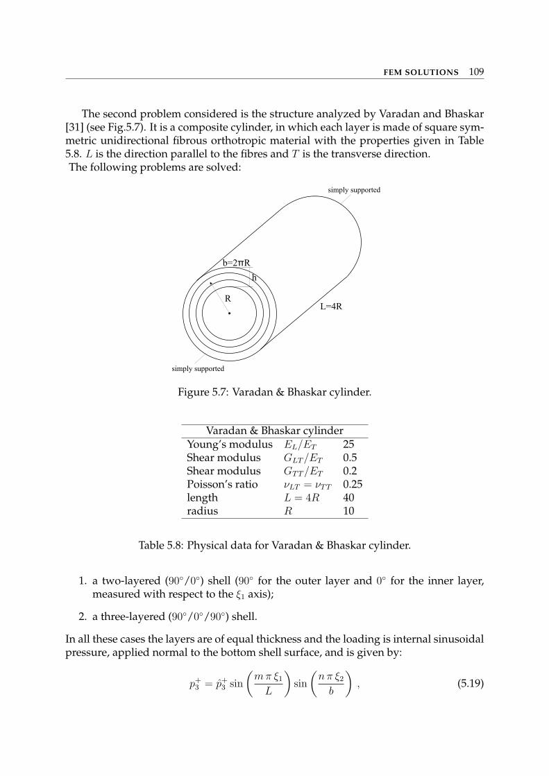
FEM SOLUTIONS 109
The second problem considered is the structure analyzed by Varadan and Bhaskar[31] (see Fig.5.7). It is a composite cylinder, in which each layer is made of square sym-metric unidirectional fibrous orthotropic material with the properties given in Table5.8. L is the direction parallel to the fibres and T is the transverse direction.The following problems are solved:
RL=4R
h
b=2 Rπ
simply supported
simply supported
Figure 5.7: Varadan & Bhaskar cylinder.
Varadan & Bhaskar cylinderYoung’s modulus EL/ET 25Shear modulus GLT /ET 0.5Shear modulus GTT /ET 0.2Poisson’s ratio νLT = νTT 0.25length L = 4R 40radius R 10
Table 5.8: Physical data for Varadan & Bhaskar cylinder.
1. a two-layered (90/0) shell (90 for the outer layer and 0 for the inner layer,measured with respect to the ξ1 axis);
2. a three-layered (90/0/90) shell.
In all these cases the layers are of equal thickness and the loading is internal sinusoidalpressure, applied normal to the bottom shell surface, and is given by:
p+3 = p+
3 sin
(mπ ξ1
L
)sin
(nπ ξ2
b
), (5.19)
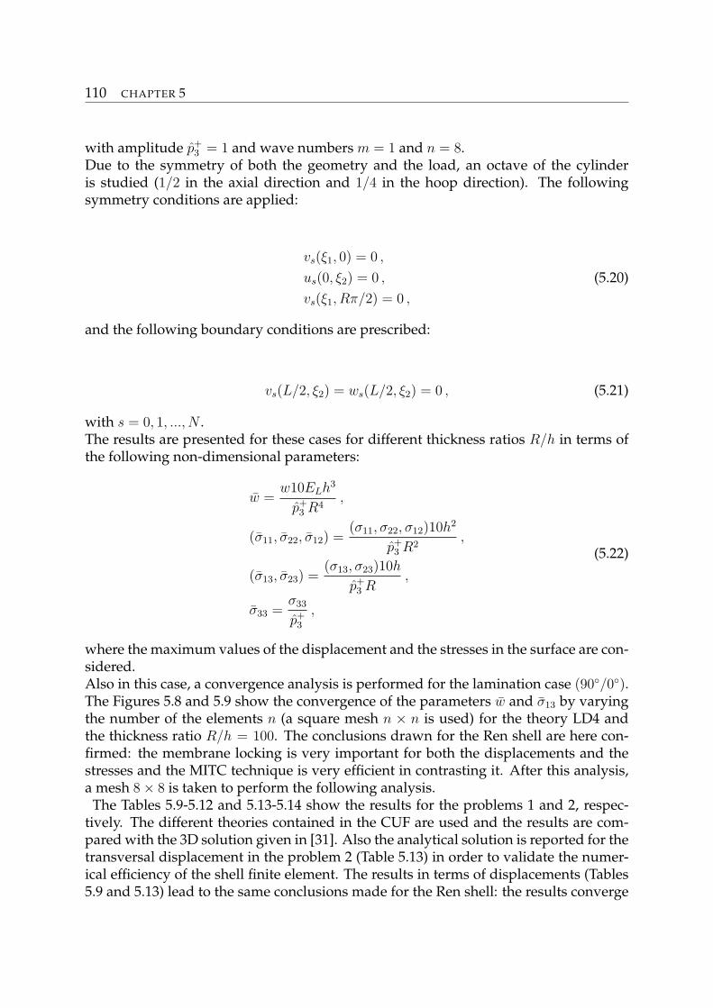
110 CHAPTER 5
with amplitude p+3 = 1 and wave numbers m = 1 and n = 8.
Due to the symmetry of both the geometry and the load, an octave of the cylinderis studied (1/2 in the axial direction and 1/4 in the hoop direction). The followingsymmetry conditions are applied:
vs(ξ1, 0) = 0 ,
us(0, ξ2) = 0 ,
vs(ξ1, Rπ/2) = 0 ,
(5.20)
and the following boundary conditions are prescribed:
vs(L/2, ξ2) = ws(L/2, ξ2) = 0 , (5.21)
with s = 0, 1, ..., N .The results are presented for these cases for different thickness ratios R/h in terms ofthe following non-dimensional parameters:
w =w10ELh3
p+3 R4
,
(σ11, σ22, σ12) =(σ11, σ22, σ12)10h2
p+3 R2
,
(σ13, σ23) =(σ13, σ23)10h
p+3 R
,
σ33 =σ33
p+3
,
(5.22)
where the maximum values of the displacement and the stresses in the surface are con-sidered.Also in this case, a convergence analysis is performed for the lamination case (90/0).The Figures 5.8 and 5.9 show the convergence of the parameters w and σ13 by varyingthe number of the elements n (a square mesh n × n is used) for the theory LD4 andthe thickness ratio R/h = 100. The conclusions drawn for the Ren shell are here con-firmed: the membrane locking is very important for both the displacements and thestresses and the MITC technique is very efficient in contrasting it. After this analysis,a mesh 8× 8 is taken to perform the following analysis.
The Tables 5.9-5.12 and 5.13-5.14 show the results for the problems 1 and 2, respec-tively. The different theories contained in the CUF are used and the results are com-pared with the 3D solution given in [31]. Also the analytical solution is reported for thetransversal displacement in the problem 2 (Table 5.13) in order to validate the numer-ical efficiency of the shell finite element. The results in terms of displacements (Tables5.9 and 5.13) lead to the same conclusions made for the Ren shell: the results converge
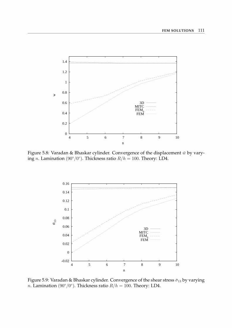
FEM SOLUTIONS 111
0
0.2
0.4
0.6
0.8
1
1.2
1.4
4 5 6 7 8 9 10
w
n
3DMITCFEMsFEM
Figure 5.8: Varadan & Bhaskar cylinder. Convergence of the displacement w by vary-ing n. Lamination (90/0). Thickness ratio R/h = 100. Theory: LD4.
-0.02
0
0.02
0.04
0.06
0.08
0.1
0.12
0.14
0.16
4 5 6 7 8 9 10
σ 13
n
3DMITCFEMsFEM
Figure 5.9: Varadan & Bhaskar cylinder. Convergence of the shear stress σ13 by varyingn. Lamination (90/0). Thickness ratio R/h = 100. Theory: LD4.
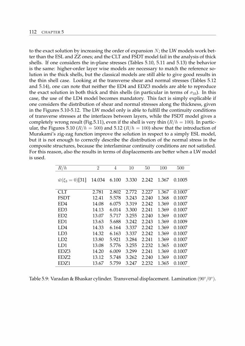
112 CHAPTER 5
to the exact solution by increasing the order of expansion N ; the LW models work bet-ter than the ESL and ZZ ones; and the CLT and FSDT model fail in the analysis of thickshells. If one considers the in-plane stresses (Tables 5.10, 5.11 and 5.13) the behavioris the same: higher-order layer wise models are necessary to match the reference so-lution in the thick shells, but the classical models are still able to give good results inthe thin shell case. Looking at the transverse shear and normal stresses (Tables 5.12and 5.14), one can note that neither the ED4 and EDZ3 models are able to reproducethe exact solution in both thick and thin shells (in particular in terms of σ33). In thiscase, the use of the LD4 model becomes mandatory. This fact is simply explicable ifone considers the distribution of shear and normal stresses along the thickness, givenin the Figures 5.10-5.12. The LW model only is able to fulfill the continuity conditionsof transverse stresses at the interfaces between layers, while the FSDT model gives acompletely wrong result (Fig.5.11), even if the shell is very thin (R/h = 100). In partic-ular, the Figures 5.10 (R/h = 500) and 5.12 (R/h = 100) show that the introduction ofMurakami’s zig-zag function improve the solution in respect to a simply ESL model,but it is not enough to correctly describe the distribution of the normal stress in thecomposite structures, because the interlaminar continuity conditions are not satisfied.For this reason, also the results in terms of displacements are better when a LW modelis used.
R/h 2 4 10 50 100 500
w(ξ3 = 0)[31] 14.034 6.100 3.330 2.242 1.367 0.1005
CLT 2.781 2.802 2.772 2.227 1.367 0.1007FSDT 12.41 5.578 3.243 2.240 1.368 0.1007ED4 14.08 6.075 3.319 2.242 1.369 0.1007ED3 14.13 6.014 3.300 2.241 1.369 0.1007ED2 13.07 5.717 3.255 2.240 1.369 0.1007ED1 13.63 5.688 3.242 2.243 1.369 0.1009LD4 14.33 6.164 3.337 2.242 1.369 0.1007LD3 14.32 6.163 3.337 2.242 1.369 0.1007LD2 13.80 5.921 3.284 2.241 1.369 0.1007LD1 13.08 5.776 3.255 2.232 1.365 0.1007EDZ3 14.20 6.009 3.299 2.241 1.369 0.1007EDZ2 13.12 5.748 3.262 2.240 1.369 0.1007EDZ1 13.67 5.759 3.247 2.232 1.365 0.1007
Table 5.9: Varadan & Bhaskar cylinder. Transversal displacement. Lamination (90/0).
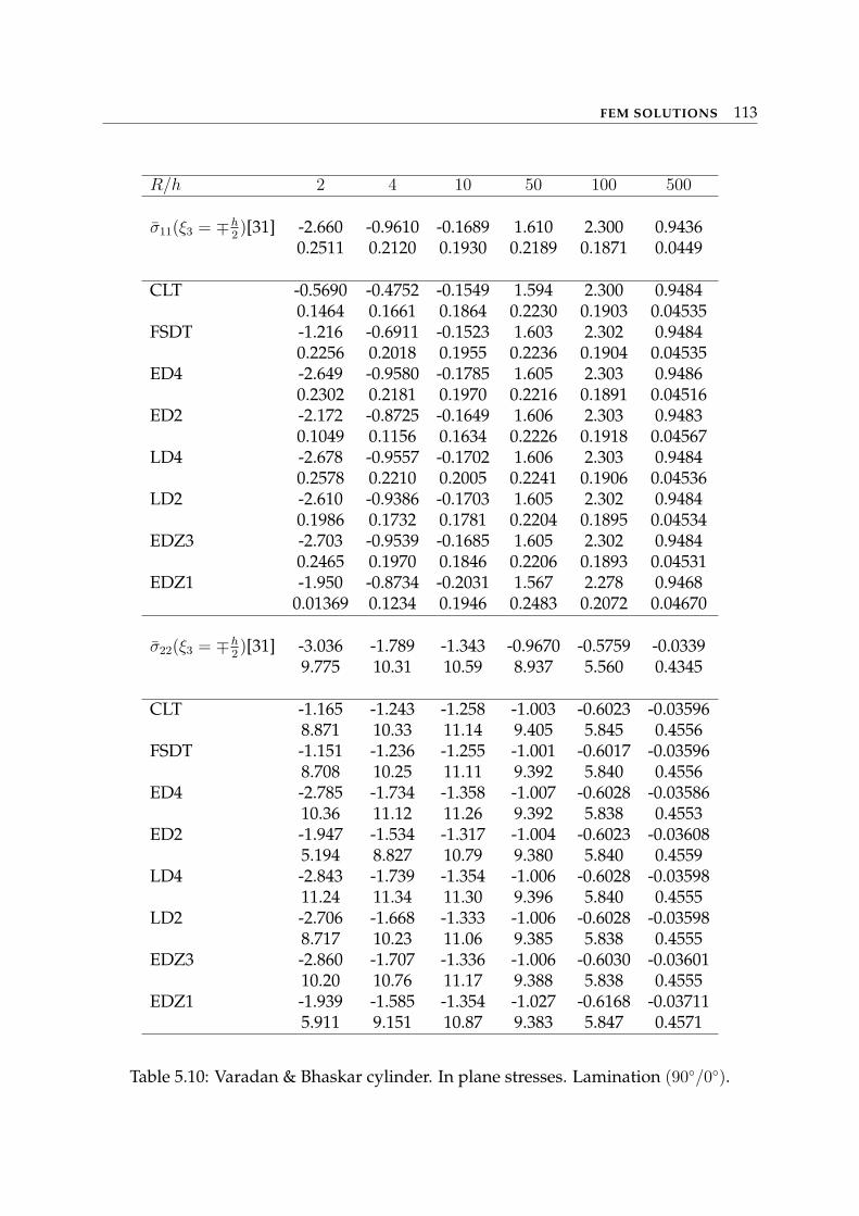
FEM SOLUTIONS 113
R/h 2 4 10 50 100 500
σ11(ξ3 = ∓h2)[31] -2.660 -0.9610 -0.1689 1.610 2.300 0.9436
0.2511 0.2120 0.1930 0.2189 0.1871 0.0449
CLT -0.5690 -0.4752 -0.1549 1.594 2.300 0.94840.1464 0.1661 0.1864 0.2230 0.1903 0.04535
FSDT -1.216 -0.6911 -0.1523 1.603 2.302 0.94840.2256 0.2018 0.1955 0.2236 0.1904 0.04535
ED4 -2.649 -0.9580 -0.1785 1.605 2.303 0.94860.2302 0.2181 0.1970 0.2216 0.1891 0.04516
ED2 -2.172 -0.8725 -0.1649 1.606 2.303 0.94830.1049 0.1156 0.1634 0.2226 0.1918 0.04567
LD4 -2.678 -0.9557 -0.1702 1.606 2.303 0.94840.2578 0.2210 0.2005 0.2241 0.1906 0.04536
LD2 -2.610 -0.9386 -0.1703 1.605 2.302 0.94840.1986 0.1732 0.1781 0.2204 0.1895 0.04534
EDZ3 -2.703 -0.9539 -0.1685 1.605 2.302 0.94840.2465 0.1970 0.1846 0.2206 0.1893 0.04531
EDZ1 -1.950 -0.8734 -0.2031 1.567 2.278 0.94680.01369 0.1234 0.1946 0.2483 0.2072 0.04670
σ22(ξ3 = ∓h2)[31] -3.036 -1.789 -1.343 -0.9670 -0.5759 -0.0339
9.775 10.31 10.59 8.937 5.560 0.4345
CLT -1.165 -1.243 -1.258 -1.003 -0.6023 -0.035968.871 10.33 11.14 9.405 5.845 0.4556
FSDT -1.151 -1.236 -1.255 -1.001 -0.6017 -0.035968.708 10.25 11.11 9.392 5.840 0.4556
ED4 -2.785 -1.734 -1.358 -1.007 -0.6028 -0.0358610.36 11.12 11.26 9.392 5.838 0.4553
ED2 -1.947 -1.534 -1.317 -1.004 -0.6023 -0.036085.194 8.827 10.79 9.380 5.840 0.4559
LD4 -2.843 -1.739 -1.354 -1.006 -0.6028 -0.0359811.24 11.34 11.30 9.396 5.840 0.4555
LD2 -2.706 -1.668 -1.333 -1.006 -0.6028 -0.035988.717 10.23 11.06 9.385 5.838 0.4555
EDZ3 -2.860 -1.707 -1.336 -1.006 -0.6030 -0.0360110.20 10.76 11.17 9.388 5.838 0.4555
EDZ1 -1.939 -1.585 -1.354 -1.027 -0.6168 -0.037115.911 9.151 10.87 9.383 5.847 0.4571
Table 5.10: Varadan & Bhaskar cylinder. In plane stresses. Lamination (90/0).
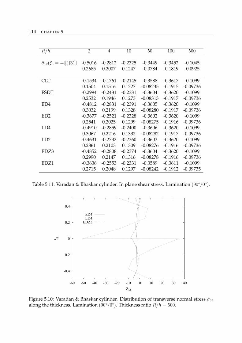
114 CHAPTER 5
R/h 2 4 10 50 100 500
σ12(ξ3 = ∓h2)[31] -0.5016 -0.2812 -0.2325 -0.3449 -0.3452 -0.1045
0.2685 0.2007 0.1247 -0.0784 -0.1819 -0.0925
CLT -0.1534 -0.1761 -0.2145 -0.3588 -0.3617 -0.10990.1504 0.1516 0.1227 -0.08235 -0.1915 -0.09736
FSDT -0.2994 -0.2431 -0.2331 -0.3604 -0.3620 -0.10990.2532 0.1946 0.1273 -0.08313 -0.1917 -0.09736
ED4 -0.4812 -0.2831 -0.2391 -0.3605 -0.3620 -0.10990.3032 0.2199 0.1328 -0.08280 -0.1917 -0.09736
ED2 -0.3677 -0.2521 -0.2328 -0.3602 -0.3620 -0.10990.2541 0.2025 0.1299 -0.08275 -0.1916 -0.09736
LD4 -0.4910 -0.2859 -0.2400 -0.3606 -0.3620 -0.10990.3067 0.2216 0.1332 -0.08282 -0.1917 -0.09736
LD2 -0.4631 -0.2732 -0.2360 -0.3603 -0.3620 -0.10990.2861 0.2103 0.1309 -0.08276 -0.1916 -0.09736
EDZ3 -0.4852 -0.2808 -0.2374 -0.3604 -0.3620 -0.10990.2990 0.2147 0.1316 -0.08278 -0.1916 -0.09736
EDZ1 -0.3636 -0.2553 -0.2331 -0.3589 -0.3611 -0.10990.2715 0.2048 0.1297 -0.08242 -0.1912 -0.09735
Table 5.11: Varadan & Bhaskar cylinder. In plane shear stress. Lamination (90/0).
-0.4
-0.2
0
0.2
0.4
-60 -50 -40 -30 -20 -10 0 10 20 30 40
ξ 3
σ33
ED4LD4
EDZ3
Figure 5.10: Varadan & Bhaskar cylinder. Distribution of transverse normal stress σ33
along the thickness. Lamination (90/0). Thickness ratio R/h = 500.
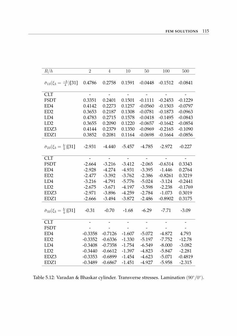
FEM SOLUTIONS 115
R/h 2 4 10 50 100 500
σ13(ξ3 = −h4
)[31] 0.4786 0.2758 0.1591 -0.0448 -0.1512 -0.0841
CLT - - - - - -FSDT 0.3351 0.2401 0.1501 -0.1111 -0.2453 -0.1229ED4 0.4142 0.2273 0.1257 -0.0560 -0.1503 -0.0797ED2 0.3653 0.2187 0.1308 -0.0781 -0.1873 -0.0963LD4 0.4783 0.2715 0.1578 -0.0418 -0.1495 -0.0843LD2 0.3655 0.2090 0.1220 -0.0657 -0.1642 -0.0854EDZ3 0.4144 0.2379 0.1350 -0.0969 -0.2165 -0.1090EDZ1 0.3852 0.2081 0.1164 -0.0698 -0.1664 -0.0856
σ23(ξ3 = h4)[31] -2.931 -4.440 -5.457 -4.785 -2.972 -0.227
CLT - - - - - -FSDT -2.664 -3.216 -3.412 -2.065 -0.6314 0.3343ED4 -2.928 -4.274 -4.931 -3.395 -1.446 0.2764ED2 -2.477 -3.392 -3.762 -2.386 -0.8261 0.3219LD4 -3.216 -4.791 -5.776 -5.024 -3.124 -0.2441LD2 -2.675 -3.671 -4.197 -3.598 -2.238 -0.1769EDZ3 -2.971 -3.896 -4.259 -2.784 -1.073 0.3019EDZ1 -2.666 -3.494 -3.872 -2.486 -0.8902 0.3175
σ33(ξ3 = h4)[31] -0.31 -0.70 -1.68 -6.29 -7.71 -3.09
CLT - - - - - -FSDT - - - - - -ED4 -0.3358 -0.7126 -1.607 -5.072 -4.872 4.793ED2 -0.3352 -0.6336 -1.330 -5.197 -7.752 -12.78LD4 -0.3408 -0.7358 -1.754 -6.549 -8.000 -3.082LD2 -0.3440 -0.6612 -1.397 -4.823 -5.847 -2.281EDZ3 -0.3353 -0.6899 -1.454 -4.623 -5.071 -0.4819EDZ1 -0.3489 -0.6867 -1.451 -4.927 -5.958 -2.315
Table 5.12: Varadan & Bhaskar cylinder. Transverse stresses. Lamination (90/0).
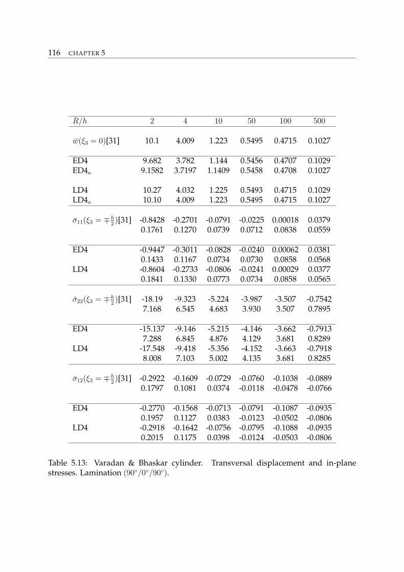
116 CHAPTER 5
R/h 2 4 10 50 100 500
w(ξ3 = 0)[31] 10.1 4.009 1.223 0.5495 0.4715 0.1027
ED4 9.682 3.782 1.144 0.5456 0.4707 0.1029ED4a 9.1582 3.7197 1.1409 0.5458 0.4708 0.1027
LD4 10.27 4.032 1.225 0.5493 0.4715 0.1029LD4a 10.10 4.009 1.223 0.5495 0.4715 0.1027
σ11(ξ3 = ∓h2)[31] -0.8428 -0.2701 -0.0791 -0.0225 0.00018 0.0379
0.1761 0.1270 0.0739 0.0712 0.0838 0.0559
ED4 -0.9447 -0.3011 -0.0828 -0.0240 0.00062 0.03810.1433 0.1167 0.0734 0.0730 0.0858 0.0568
LD4 -0.8604 -0.2733 -0.0806 -0.0241 0.00029 0.03770.1841 0.1330 0.0773 0.0734 0.0858 0.0565
σ22(ξ3 = ∓h2)[31] -18.19 -9.323 -5.224 -3.987 -3.507 -0.7542
7.168 6.545 4.683 3.930 3.507 0.7895
ED4 -15.137 -9.146 -5.215 -4.146 -3.662 -0.79137.288 6.845 4.876 4.129 3.681 0.8289
LD4 -17.548 -9.418 -5.356 -4.152 -3.663 -0.79188.008 7.103 5.002 4.135 3.681 0.8285
σ12(ξ3 = ∓h2)[31] -0.2922 -0.1609 -0.0729 -0.0760 -0.1038 -0.0889
0.1797 0.1081 0.0374 -0.0118 -0.0478 -0.0766
ED4 -0.2770 -0.1568 -0.0713 -0.0791 -0.1087 -0.09350.1957 0.1127 0.0383 -0.0123 -0.0502 -0.0806
LD4 -0.2918 -0.1642 -0.0756 -0.0795 -0.1088 -0.09350.2015 0.1175 0.0398 -0.0124 -0.0503 -0.0806
Table 5.13: Varadan & Bhaskar cylinder. Transversal displacement and in-planestresses. Lamination (90/0/90).
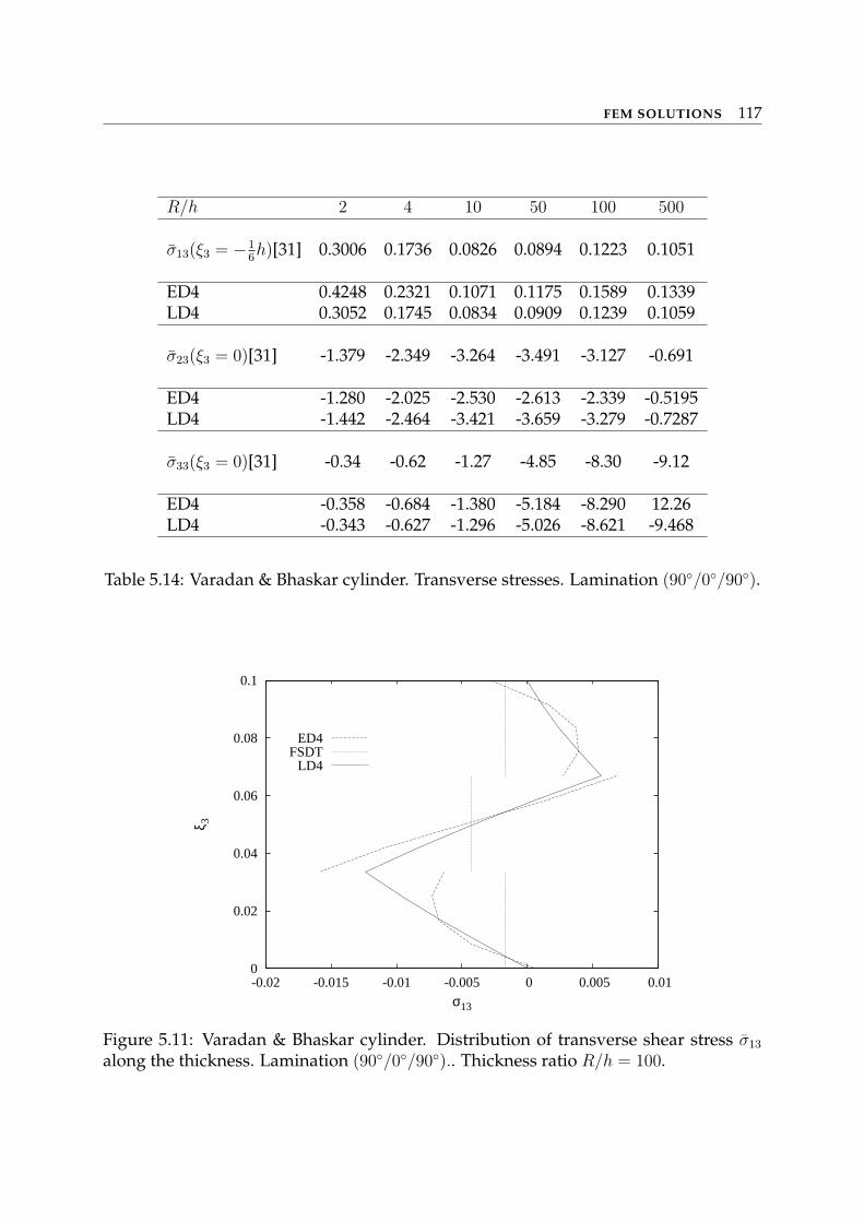
FEM SOLUTIONS 117
R/h 2 4 10 50 100 500
σ13(ξ3 = −16h)[31] 0.3006 0.1736 0.0826 0.0894 0.1223 0.1051
ED4 0.4248 0.2321 0.1071 0.1175 0.1589 0.1339LD4 0.3052 0.1745 0.0834 0.0909 0.1239 0.1059
σ23(ξ3 = 0)[31] -1.379 -2.349 -3.264 -3.491 -3.127 -0.691
ED4 -1.280 -2.025 -2.530 -2.613 -2.339 -0.5195LD4 -1.442 -2.464 -3.421 -3.659 -3.279 -0.7287
σ33(ξ3 = 0)[31] -0.34 -0.62 -1.27 -4.85 -8.30 -9.12
ED4 -0.358 -0.684 -1.380 -5.184 -8.290 12.26LD4 -0.343 -0.627 -1.296 -5.026 -8.621 -9.468
Table 5.14: Varadan & Bhaskar cylinder. Transverse stresses. Lamination (90/0/90).
0
0.02
0.04
0.06
0.08
0.1
-0.02 -0.015 -0.01 -0.005 0 0.005 0.01
ξ 3
σ13
ED4FSDT
LD4
Figure 5.11: Varadan & Bhaskar cylinder. Distribution of transverse shear stress σ13
along the thickness. Lamination (90/0/90).. Thickness ratio R/h = 100.
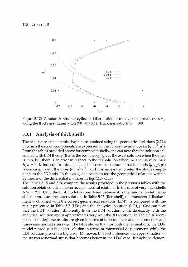
118 CHAPTER 5
0
0.02
0.04
0.06
0.08
0.1
-12 -10 -8 -6 -4 -2 0 2
ξ 3
σ33
ED4EDZ4
LD4
Figure 5.12: Varadan & Bhaskar cylinder. Distribution of transverse normal stress σ33
along the thickness. Lamination (90/0/90). Thickness ratio R/h = 100.
5.3.1 Analysis of thick shells
The results presented in this chapter are obtained using the geometrical relations (2.21),in which the strain components are expressed in the 3D contravariant basis (g1, g2, g3).From the tables provided above for composite shells, one can note that the solution cal-culated with LD4 theory (that is the best theory) gives the exact solution when the shellis thin, but there is an error in respect to the 3D solution when the shell is very thickR/h = 2, 4. Indeed, for thick shells, it isn’t correct to assume that the basis (g1, g2, g3)is coincident with the basis (a1,a2, a3), and it is necessary to refer the strain compo-nents to the 2D basis. In this case, one needs to use the geometrical relations writtenby means of the differential matrixes in Eqs.(2.27-2.28).The Tables 5.15 and 5.16 compare the results provided in the previous tables with thesolution obtained using the correct geometrical relations, in the case of very thick shellsR/h = 2, 4. Only the LD4 model is considered because it is the unique model that isable to reproduce the exact solution. In Table 5.15 (Ren shell), the transversal displace-ment w obtained with the correct geometrical relations (LD4’), is compared with theresult presented in Table 5.7 (LD4) and the analytical solution (LD4a). One can notethat the LD4’ solution, differently from the LD4 solution, coincide exactly with theanalytical solution and it approximates very well the 3D solution. In Table 5.16 (com-posite cylinder), the results are given in terms of both transversal displacement w andtransverse normal stress σ33. The table shows that, for both the laminations, the LD4’model reproduces the exact solution in terms of transversal displacement, while theLD4 solution presents a big error. Moreover, this fact influences the approximation ofthe trasverse normal stress that becomes better in the LD4’ case. It might be demon-
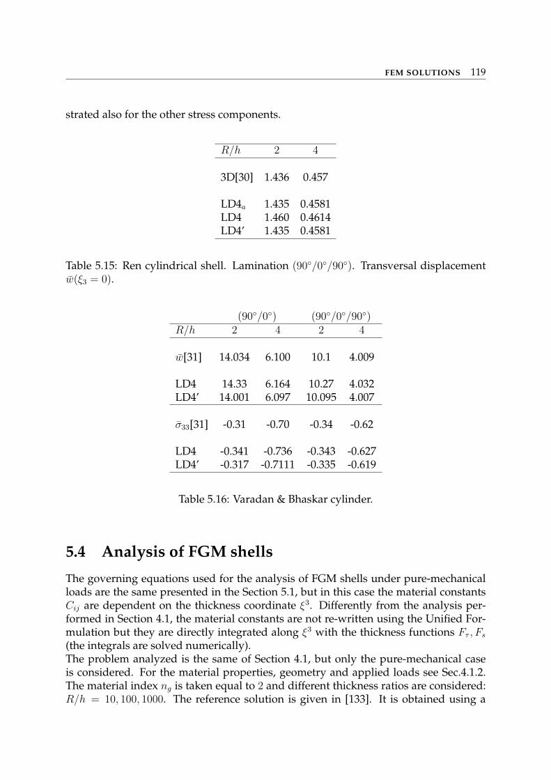
FEM SOLUTIONS 119
strated also for the other stress components.
R/h 2 4
3D[30] 1.436 0.457
LD4a 1.435 0.4581LD4 1.460 0.4614LD4’ 1.435 0.4581
Table 5.15: Ren cylindrical shell. Lamination (90/0/90). Transversal displacementw(ξ3 = 0).
(90/0) (90/0/90)R/h 2 4 2 4
w[31] 14.034 6.100 10.1 4.009
LD4 14.33 6.164 10.27 4.032LD4’ 14.001 6.097 10.095 4.007
σ33[31] -0.31 -0.70 -0.34 -0.62
LD4 -0.341 -0.736 -0.343 -0.627LD4’ -0.317 -0.7111 -0.335 -0.619
Table 5.16: Varadan & Bhaskar cylinder.
5.4 Analysis of FGM shells
The governing equations used for the analysis of FGM shells under pure-mechanicalloads are the same presented in the Section 5.1, but in this case the material constantsCij are dependent on the thickness coordinate ξ3. Differently from the analysis per-formed in Section 4.1, the material constants are not re-written using the Unified For-mulation but they are directly integrated along ξ3 with the thickness functions Fτ , Fs
(the integrals are solved numerically).The problem analyzed is the same of Section 4.1, but only the pure-mechanical caseis considered. For the material properties, geometry and applied loads see Sec.4.1.2.The material index ng is taken equal to 2 and different thickness ratios are considered:R/h = 10, 100, 1000. The reference solution is given in [133]. It is obtained using a
120 CHAPTER 5
fourth-order CUF theory and taking a very high number of fictitious layers (Nl = 100)in the FGM shell, in which the mechanical properties are considered constant alongthe thickness and equal to the mean value between the top and bottom of the layer. In[133], it has been demonstrated that this procedure permits to calculate the quasi-3Dsolution of the static problem in FGM structures.Table 5.17 shows the results in terms of displacements u and w and Table 5.18 in termsof the stresses σ22, σ13 and σ33. The comparison of FEM results, obtained with the dif-ferent theories contained in the CUF, with the quasi-3D solution shows that the CUF el-ement works very well for the analysis of FGM shells. It is demonstrated that a fourth-order of expansion of the displacements is necessary to ensure the convergence of thesolution. The element provides very good results also for very thin shells (R/h = 1000)in spite of the membrane and shear locking phenomenon that usually affects the shellfinite elements. One can note that the FSDT model is not able to accurately describe thedistribution of displacements and stresses because it doesn’t consider the variability ofthe mechanical behavior in FGMs along the thickness.As discussed in [133], the influence of the material gradient on the variation of thetransversal displacement is more evident in the thermal analysis and the use of higher-order models becomes mandatory in that case. For these reasons, a future work willbe dedicated to the thermal analysis of functionally graded plates and shells by meansof the CUF shell element.For more details about the analysis of FGM structures by means of the CUF MITC9
shell element, one can refer to [227].
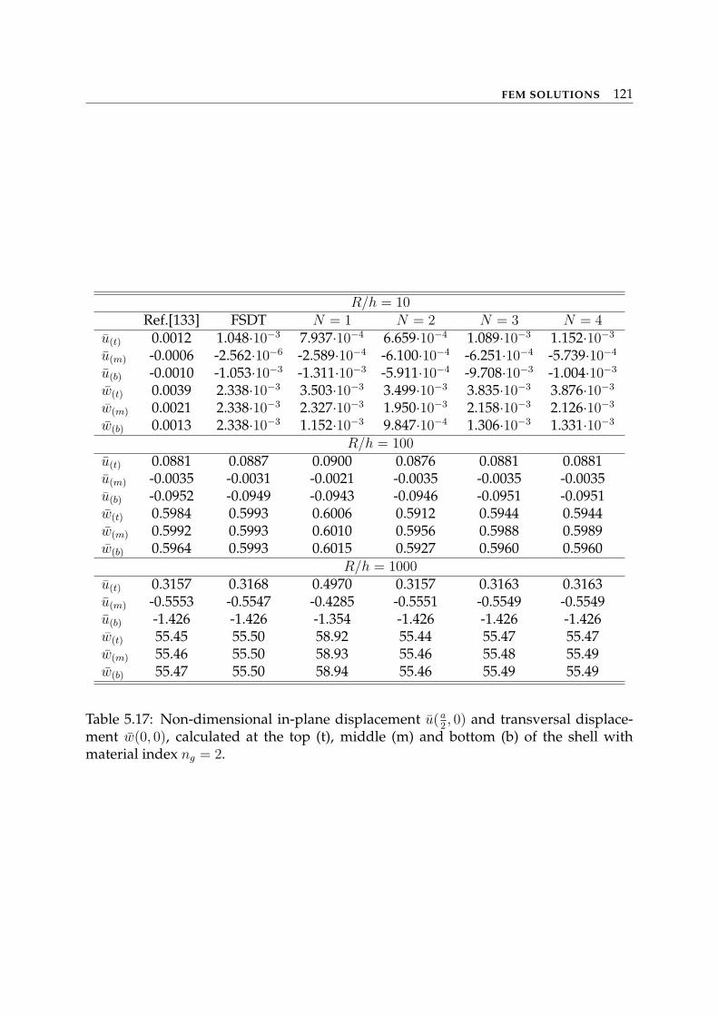
FEM SOLUTIONS 121
R/h = 10Ref.[133] FSDT N = 1 N = 2 N = 3 N = 4
u(t) 0.0012 1.048·10−3 7.937·10−4 6.659·10−4 1.089·10−3 1.152·10−3
u(m) -0.0006 -2.562·10−6 -2.589·10−4 -6.100·10−4 -6.251·10−4 -5.739·10−4
u(b) -0.0010 -1.053·10−3 -1.311·10−3 -5.911·10−4 -9.708·10−3 -1.004·10−3
w(t) 0.0039 2.338·10−3 3.503·10−3 3.499·10−3 3.835·10−3 3.876·10−3
w(m) 0.0021 2.338·10−3 2.327·10−3 1.950·10−3 2.158·10−3 2.126·10−3
w(b) 0.0013 2.338·10−3 1.152·10−3 9.847·10−4 1.306·10−3 1.331·10−3
R/h = 100u(t) 0.0881 0.0887 0.0900 0.0876 0.0881 0.0881u(m) -0.0035 -0.0031 -0.0021 -0.0035 -0.0035 -0.0035u(b) -0.0952 -0.0949 -0.0943 -0.0946 -0.0951 -0.0951w(t) 0.5984 0.5993 0.6006 0.5912 0.5944 0.5944w(m) 0.5992 0.5993 0.6010 0.5956 0.5988 0.5989w(b) 0.5964 0.5993 0.6015 0.5927 0.5960 0.5960
R/h = 1000u(t) 0.3157 0.3168 0.4970 0.3157 0.3163 0.3163u(m) -0.5553 -0.5547 -0.4285 -0.5551 -0.5549 -0.5549u(b) -1.426 -1.426 -1.354 -1.426 -1.426 -1.426w(t) 55.45 55.50 58.92 55.44 55.47 55.47w(m) 55.46 55.50 58.93 55.46 55.48 55.49w(b) 55.47 55.50 58.94 55.46 55.49 55.49
Table 5.17: Non-dimensional in-plane displacement u(a2, 0) and transversal displace-
ment w(0, 0), calculated at the top (t), middle (m) and bottom (b) of the shell withmaterial index ng = 2.
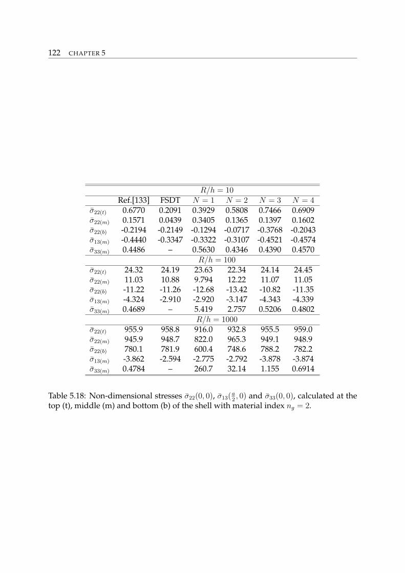
122 CHAPTER 5
R/h = 10Ref.[133] FSDT N = 1 N = 2 N = 3 N = 4
σ22(t) 0.6770 0.2091 0.3929 0.5808 0.7466 0.6909σ22(m) 0.1571 0.0439 0.3405 0.1365 0.1397 0.1602σ22(b) -0.2194 -0.2149 -0.1294 -0.0717 -0.3768 -0.2043σ13(m) -0.4440 -0.3347 -0.3322 -0.3107 -0.4521 -0.4574σ33(m) 0.4486 – 0.5630 0.4346 0.4390 0.4570
R/h = 100σ22(t) 24.32 24.19 23.63 22.34 24.14 24.45σ22(m) 11.03 10.88 9.794 12.22 11.07 11.05σ22(b) -11.22 -11.26 -12.68 -13.42 -10.82 -11.35σ13(m) -4.324 -2.910 -2.920 -3.147 -4.343 -4.339σ33(m) 0.4689 – 5.419 2.757 0.5206 0.4802
R/h = 1000σ22(t) 955.9 958.8 916.0 932.8 955.5 959.0σ22(m) 945.9 948.7 822.0 965.3 949.1 948.9σ22(b) 780.1 781.9 600.4 748.6 788.2 782.2σ13(m) -3.862 -2.594 -2.775 -2.792 -3.878 -3.874σ33(m) 0.4784 – 260.7 32.14 1.155 0.6914
Table 5.18: Non-dimensional stresses σ22(0, 0), σ13(a2, 0) and σ33(0, 0), calculated at the
top (t), middle (m) and bottom (b) of the shell with material index ng = 2.
Chapter 6
RBF solutions
In this chapter, some results obtained from the analysis of composite and FGM shells by meansof the Radial Basis Functions method are presented. The governing equations are derived instrong form from the PVD for the static analysis and the free vibration analysis of shells. Notethat every calculation is made referring to the double-curvature geometry and relative notation(see Section 2.2.1), even when the shell is cylindrical. Only the pure-mechanical problem isconsidered. New theories, different from those presented in Chapter 2, are used for the analysis.These are the Sinusoidal Shear Deformation Theory (SSDT) and the High-order Shear Defor-mation Theory (HSDT) and they are implemented by means of the Unified Formulation. Theresults are compared with analytical solutions given in literature and they show that the RBFmethod is very efficient for the study of both composite and FGM structures. Also a compar-ison with FEM results is provided in order to prove the advantages of radial basis functionsthat are the absence of mesh, the ease of discretization of boundary conditions and equations ofequilibrium.
6.1 Governing equations
The differential equations for the analysis of doubly-curved shells by means of the RBFmethod are obtained following the procedure exposed in Section 3.1. The geometricalrelations (Eqs.(2.29)), the constitutive equations (Eqs.(2.36)) and the Unified Formula-tion (Eqs.(2.1)) are substituted in the PVD (Eq.3.2) and the integration by parts (seeEq.(3.9) is applied in order to calculate the strong solution. The final compact form ofgoverning equations and relative boundary conditions is given in the equations (5.3)and (3.15), respectively. The explicit expression of the fundamental nuclei Kkτs
uu , Πkτsuu
123
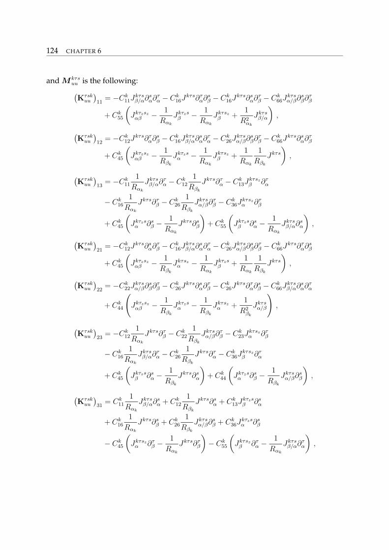
124 CHAPTER 6
and M kτsuu is the following:(Kτsk
uu
)11
= −Ck11J
kτsβ/α∂s
α∂τα − Ck
16Jkτs∂τ
α∂sβ − Ck
16Jkτs∂s
α∂τβ − Ck
66Jkτsα/β∂s
β∂τβ
+ Ck55
(Jkτzsz
αβ − 1
Rαk
Jkτzsβ − 1
Rαk
Jkτszβ +
1
R2αk
Jkτsβ/α
),
(Kτsk
uu
)12
= −Ck12J
kτs∂τα∂s
β − Ck16J
kτsβ/α∂s
α∂τα − Ck
26Jkτsα/β∂s
β∂τβ − Ck
66Jkτs∂s
α∂τβ
+ Ck45
(Jkτzsz
αβ − 1
Rβk
Jkτzsα − 1
Rαk
Jkτszβ +
1
Rαk
1
Rβk
Jkτs
),
(Kτsk
uu
)13
= −Ck11
1
Rαk
Jkτsβ/α∂τ
α − Ck12
1
Rβk
Jkτs∂τα − Ck
13Jkτszβ ∂τ
α
− Ck16
1
Rαk
Jkτs∂τβ − Ck
26
1
Rβk
Jkτsα/β∂τ
β − Ck36J
kτszα ∂τ
β
+ Ck45
(Jkτzs
α ∂sβ −
1
Rαk
Jkτs∂sβ
)+ Ck
55
(Jkτzs
β ∂sα −
1
Rαk
Jkτsβ/α∂s
α
),
(Kτsk
uu
)21
= −Ck12J
kτs∂sα∂τ
β − Ck16J
kτsβ/α∂s
α∂τα − Ck
26Jkτsα/β∂s
β∂τβ − Ck
66Jkτs∂τ
α∂sβ
+ Ck45
(Jkτzsz
αβ − 1
Rβk
Jkτszα − 1
Rαk
Jkτzsβ +
1
Rαk
1
Rβk
Jkτs
),
(Kτsk
uu
)22
= −Ck22J
kτsα/β∂s
β∂τβ − Ck
26Jkτs∂s
α∂τβ − Ck
26Jkτs∂τ
α∂sβ − Ck
66Jkτsβ/α∂s
α∂τα
+ Ck44
(Jkτzsz
αβ − 1
Rβk
Jkτzsα − 1
Rβk
Jkτszα +
1
R2βk
Jkτsα/β
),
(Kτsk
uu
)23
= −Ck12
1
Rαk
Jkτs∂τβ − Ck
22
1
Rβk
Jkτsα/β∂τ
β − Ck23J
kτszα ∂τ
β
− Ck16
1
Rαk
Jkτsβ/α∂τ
α − Ck26
1
Rβk
Jkτs∂τα − Ck
36Jkτszβ ∂τ
α
+ Ck45
(Jkτzs
β ∂sα −
1
Rβk
Jkτs∂sα
)+ Ck
44
(Jkτzs
α ∂sβ −
1
Rβk
Jkτsα/β∂s
β
),
(Kτsk
uu
)31
= Ck11
1
Rαk
Jkτsβ/α∂s
α + Ck12
1
Rβk
Jkτs∂sα + Ck
13Jkτzsβ ∂s
α
+ Ck16
1
Rαk
Jkτs∂sβ + Ck
26
1
Rβk
Jkτsα/β∂s
β + Ck36J
kτzsα ∂s
β
− Ck45
(Jkτsz
α ∂τβ −
1
Rαk
Jkτs∂τβ
)− Ck
55
(Jkτsz
β ∂τα −
1
Rαk
Jkτsβ/α∂τ
α
),
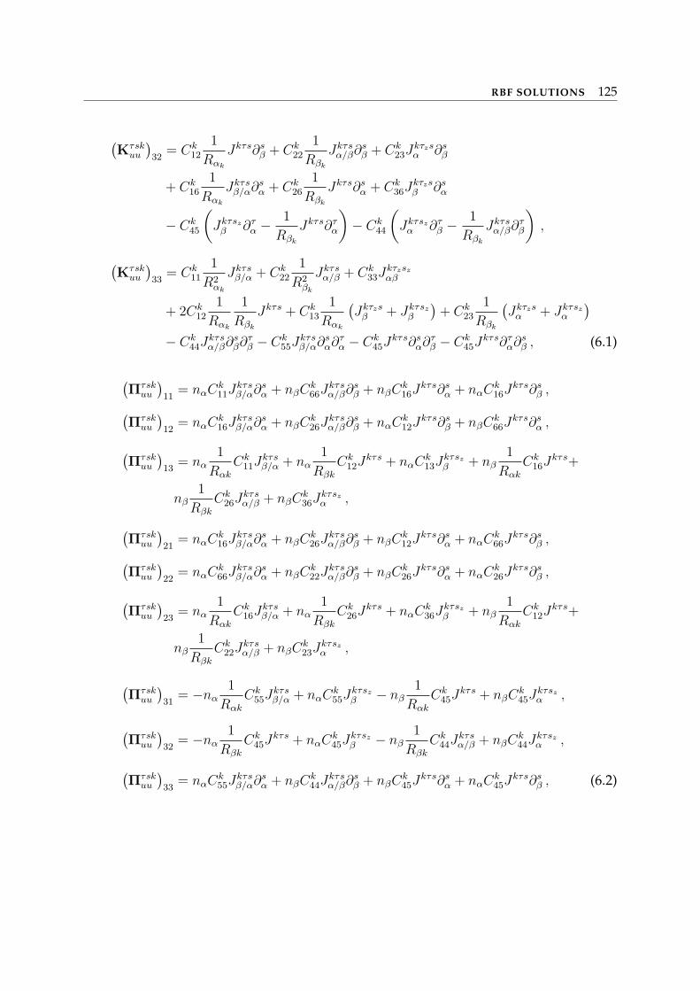
RBF SOLUTIONS 125
(Kτsk
uu
)32
= Ck12
1
Rαk
Jkτs∂sβ + Ck
22
1
Rβk
Jkτsα/β∂s
β + Ck23J
kτzsα ∂s
β
+ Ck16
1
Rαk
Jkτsβ/α∂s
α + Ck26
1
Rβk
Jkτs∂sα + Ck
36Jkτzsβ ∂s
α
− Ck45
(Jkτsz
β ∂τα −
1
Rβk
Jkτs∂τα
)− Ck
44
(Jkτsz
α ∂τβ −
1
Rβk
Jkτsα/β∂τ
β
),
(Kτsk
uu
)33
= Ck11
1
R2αk
Jkτsβ/α + Ck
22
1
R2βk
Jkτsα/β + Ck
33Jkτzszαβ
+ 2Ck12
1
Rαk
1
Rβk
Jkτs + Ck13
1
Rαk
(Jkτzs
β + Jkτszβ
)+ Ck
23
1
Rβk
(Jkτzs
α + Jkτszα
)
− Ck44J
kτsα/β∂s
β∂τβ − Ck
55Jkτsβ/α∂s
α∂τα − Ck
45Jkτs∂s
α∂τβ − Ck
45Jkτs∂τ
α∂sβ , (6.1)
(Πτsk
uu
)11
= nαCk11J
kτsβ/α∂s
α + nβCk66J
kτsα/β∂s
β + nβCk16J
kτs∂sα + nαCk
16Jkτs∂s
β ,
(Πτsk
uu
)12
= nαCk16J
kτsβ/α∂s
α + nβCk26J
kτsα/β∂s
β + nαCk12J
kτs∂sβ + nβCk
66Jkτs∂s
α ,
(Πτsk
uu
)13
= nα1
Rαk
Ck11J
kτsβ/α + nα
1
Rβk
Ck12J
kτs + nαCk13J
kτszβ + nβ
1
Rαk
Ck16J
kτs+
nβ1
Rβk
Ck26J
kτsα/β + nβCk
36Jkτszα ,
(Πτsk
uu
)21
= nαCk16J
kτsβ/α∂s
α + nβCk26J
kτsα/β∂s
β + nβCk12J
kτs∂sα + nαCk
66Jkτs∂s
β ,
(Πτsk
uu
)22
= nαCk66J
kτsβ/α∂s
α + nβCk22J
kτsα/β∂s
β + nβCk26J
kτs∂sα + nαCk
26Jkτs∂s
β ,
(Πτsk
uu
)23
= nα1
Rαk
Ck16J
kτsβ/α + nα
1
Rβk
Ck26J
kτs + nαCk36J
kτszβ + nβ
1
Rαk
Ck12J
kτs+
nβ1
Rβk
Ck22J
kτsα/β + nβCk
23Jkτszα ,
(Πτsk
uu
)31
= −nα1
Rαk
Ck55J
kτsβ/α + nαCk
55Jkτszβ − nβ
1
Rαk
Ck45J
kτs + nβCk45J
kτszα ,
(Πτsk
uu
)32
= −nα1
Rβk
Ck45J
kτs + nαCk45J
kτszβ − nβ
1
Rβk
Ck44J
kτsα/β + nβCk
44Jkτszα ,
(Πτsk
uu
)33
= nαCk55J
kτsβ/α∂s
α + nβCk44J
kτsα/β∂s
β + nβCk45J
kτs∂sα + nαCk
45Jkτs∂s
β , (6.2)
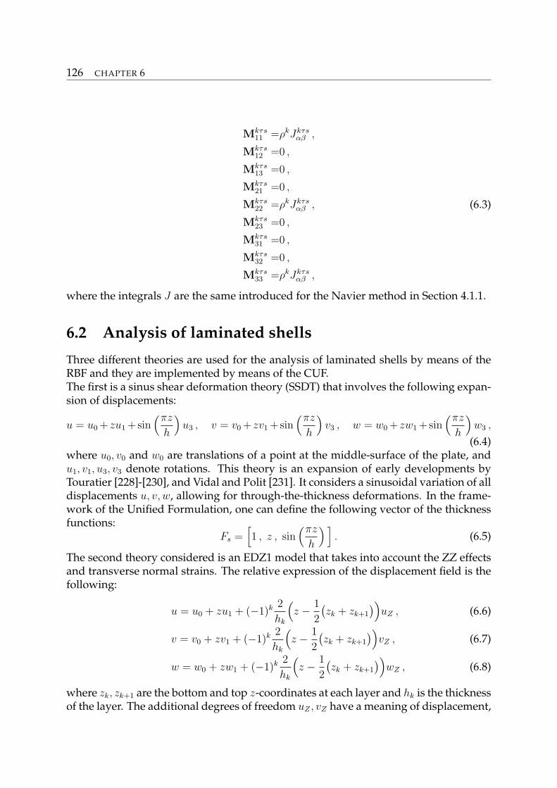
126 CHAPTER 6
Mkτs11 =ρkJkτs
αβ ,
Mkτs12 =0 ,
Mkτs13 =0 ,
Mkτs21 =0 ,
Mkτs22 =ρkJkτs
αβ ,
Mkτs23 =0 ,
Mkτs31 =0 ,
Mkτs32 =0 ,
Mkτs33 =ρkJkτs
αβ ,
(6.3)
where the integrals J are the same introduced for the Navier method in Section 4.1.1.
6.2 Analysis of laminated shells
Three different theories are used for the analysis of laminated shells by means of theRBF and they are implemented by means of the CUF.The first is a sinus shear deformation theory (SSDT) that involves the following expan-sion of displacements:
u = u0 + zu1 +sin(πz
h
)u3 , v = v0 + zv1 +sin
(πz
h
)v3 , w = w0 + zw1 +sin
(πz
h
)w3 ,
(6.4)where u0, v0 and w0 are translations of a point at the middle-surface of the plate, andu1, v1, u3, v3 denote rotations. This theory is an expansion of early developments byTouratier [228]-[230], and Vidal and Polit [231]. It considers a sinusoidal variation of alldisplacements u, v, w, allowing for through-the-thickness deformations. In the frame-work of the Unified Formulation, one can define the following vector of the thicknessfunctions:
Fs =[1 , z , sin
(πz
h
) ]. (6.5)
The second theory considered is an EDZ1 model that takes into account the ZZ effectsand transverse normal strains. The relative expression of the displacement field is thefollowing:
u = u0 + zu1 + (−1)k 2
hk
(z − 1
2
(zk + zk+1
))uZ , (6.6)
v = v0 + zv1 + (−1)k 2
hk
(z − 1
2
(zk + zk+1
))vZ , (6.7)
w = w0 + zw1 + (−1)k 2
hk
(z − 1
2
(zk + zk+1
))wZ , (6.8)
where zk, zk+1 are the bottom and top z-coordinates at each layer and hk is the thicknessof the layer. The additional degrees of freedom uZ , vZ have a meaning of displacement,
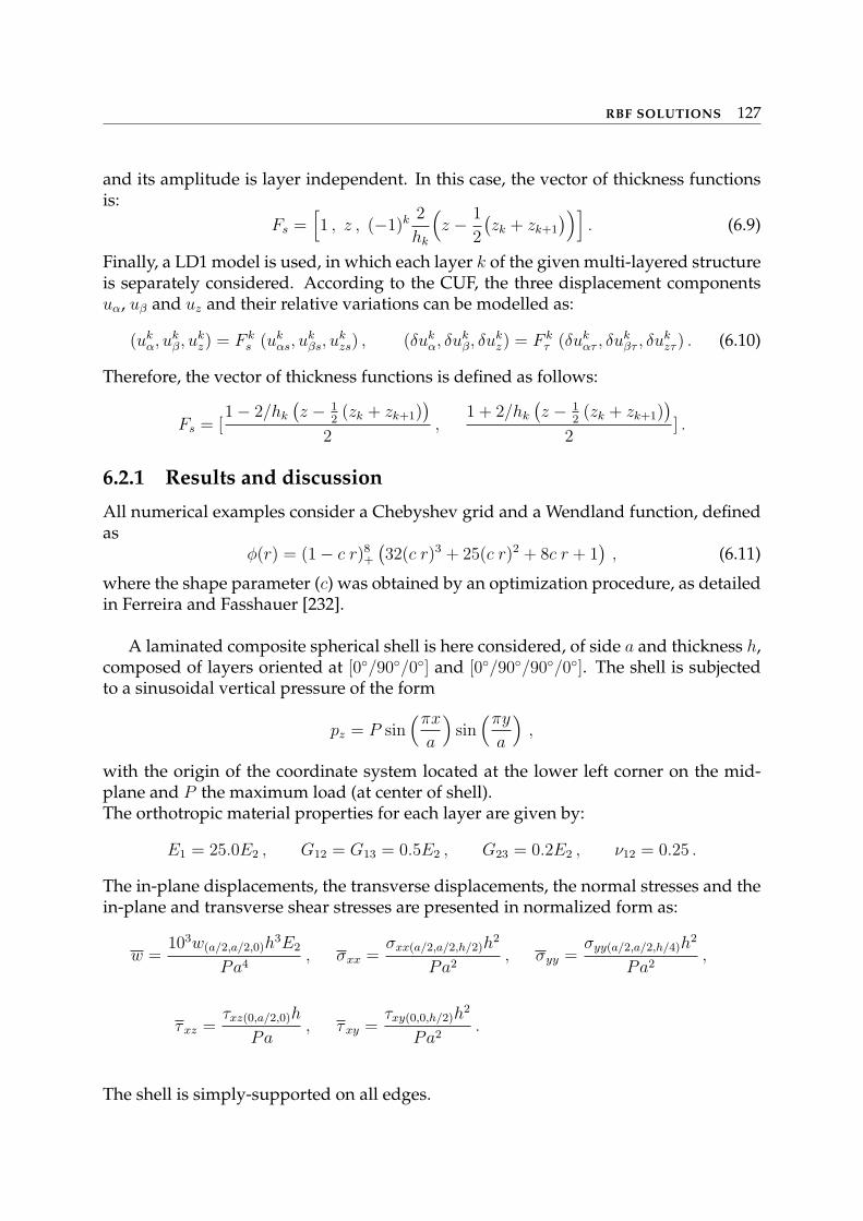
RBF SOLUTIONS 127
and its amplitude is layer independent. In this case, the vector of thickness functionsis:
Fs =[1 , z , (−1)k 2
hk
(z − 1
2
(zk + zk+1
))]. (6.9)
Finally, a LD1 model is used, in which each layer k of the given multi-layered structureis separately considered. According to the CUF, the three displacement componentsuα, uβ and uz and their relative variations can be modelled as:
(ukα, uk
β, ukz) = F k
s (ukαs, u
kβs, u
kzs) , (δuk
α, δukβ, δuk
z) = F kτ (δuk
ατ , δukβτ , δu
kzτ ) . (6.10)
Therefore, the vector of thickness functions is defined as follows:
Fs = [1− 2/hk
(z − 1
2(zk + zk+1)
)
2,
1 + 2/hk
(z − 1
2(zk + zk+1)
)
2] .
6.2.1 Results and discussion
All numerical examples consider a Chebyshev grid and a Wendland function, definedas
φ(r) = (1− c r)8+
(32(c r)3 + 25(c r)2 + 8c r + 1
), (6.11)
where the shape parameter (c) was obtained by an optimization procedure, as detailedin Ferreira and Fasshauer [232].
A laminated composite spherical shell is here considered, of side a and thickness h,composed of layers oriented at [0/90/0] and [0/90/90/0]. The shell is subjectedto a sinusoidal vertical pressure of the form
pz = P sin(πx
a
)sin
(πy
a
),
with the origin of the coordinate system located at the lower left corner on the mid-plane and P the maximum load (at center of shell).The orthotropic material properties for each layer are given by:
E1 = 25.0E2 , G12 = G13 = 0.5E2 , G23 = 0.2E2 , ν12 = 0.25 .
The in-plane displacements, the transverse displacements, the normal stresses and thein-plane and transverse shear stresses are presented in normalized form as:
w =103w(a/2,a/2,0)h
3E2
Pa4, σxx =
σxx(a/2,a/2,h/2)h2
Pa2, σyy =
σyy(a/2,a/2,h/4)h2
Pa2,
τxz =τxz(0,a/2,0)h
Pa, τxy =
τxy(0,0,h/2)h2
Pa2.
The shell is simply-supported on all edges.
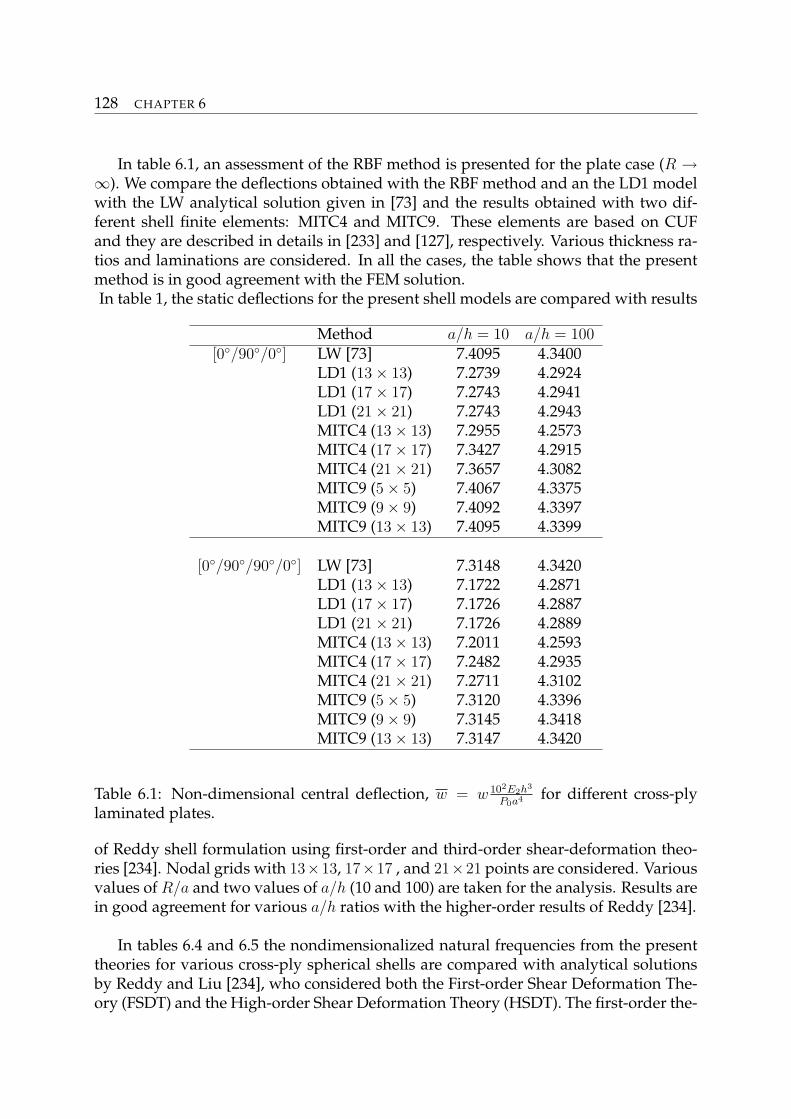
128 CHAPTER 6
In table 6.1, an assessment of the RBF method is presented for the plate case (R →∞). We compare the deflections obtained with the RBF method and an the LD1 modelwith the LW analytical solution given in [73] and the results obtained with two dif-ferent shell finite elements: MITC4 and MITC9. These elements are based on CUFand they are described in details in [233] and [127], respectively. Various thickness ra-tios and laminations are considered. In all the cases, the table shows that the presentmethod is in good agreement with the FEM solution.In table 1, the static deflections for the present shell models are compared with results
Method a/h = 10 a/h = 100[0/90/0] LW [73] 7.4095 4.3400
LD1 (13× 13) 7.2739 4.2924LD1 (17× 17) 7.2743 4.2941LD1 (21× 21) 7.2743 4.2943MITC4 (13× 13) 7.2955 4.2573MITC4 (17× 17) 7.3427 4.2915MITC4 (21× 21) 7.3657 4.3082MITC9 (5× 5) 7.4067 4.3375MITC9 (9× 9) 7.4092 4.3397MITC9 (13× 13) 7.4095 4.3399
[0/90/90/0] LW [73] 7.3148 4.3420LD1 (13× 13) 7.1722 4.2871LD1 (17× 17) 7.1726 4.2887LD1 (21× 21) 7.1726 4.2889MITC4 (13× 13) 7.2011 4.2593MITC4 (17× 17) 7.2482 4.2935MITC4 (21× 21) 7.2711 4.3102MITC9 (5× 5) 7.3120 4.3396MITC9 (9× 9) 7.3145 4.3418MITC9 (13× 13) 7.3147 4.3420
Table 6.1: Non-dimensional central deflection, w = w 102E2h3
P0a4 for different cross-plylaminated plates.
of Reddy shell formulation using first-order and third-order shear-deformation theo-ries [234]. Nodal grids with 13×13, 17×17 , and 21×21 points are considered. Variousvalues of R/a and two values of a/h (10 and 100) are taken for the analysis. Results arein good agreement for various a/h ratios with the higher-order results of Reddy [234].
In tables 6.4 and 6.5 the nondimensionalized natural frequencies from the presenttheories for various cross-ply spherical shells are compared with analytical solutionsby Reddy and Liu [234], who considered both the First-order Shear Deformation The-ory (FSDT) and the High-order Shear Deformation Theory (HSDT). The first-order the-
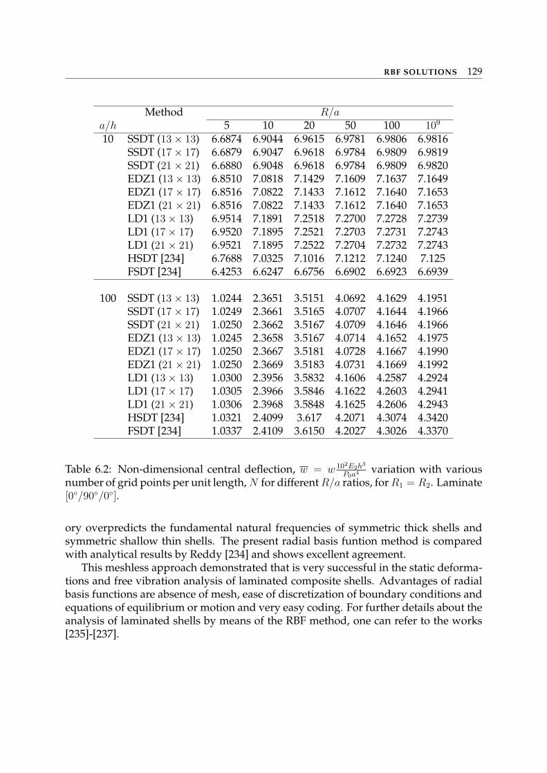
RBF SOLUTIONS 129
Method R/aa/h 5 10 20 50 100 109
10 SSDT (13× 13) 6.6874 6.9044 6.9615 6.9781 6.9806 6.9816SSDT (17× 17) 6.6879 6.9047 6.9618 6.9784 6.9809 6.9819SSDT (21× 21) 6.6880 6.9048 6.9618 6.9784 6.9809 6.9820EDZ1 (13× 13) 6.8510 7.0818 7.1429 7.1609 7.1637 7.1649EDZ1 (17× 17) 6.8516 7.0822 7.1433 7.1612 7.1640 7.1653EDZ1 (21× 21) 6.8516 7.0822 7.1433 7.1612 7.1640 7.1653LD1 (13× 13) 6.9514 7.1891 7.2518 7.2700 7.2728 7.2739LD1 (17× 17) 6.9520 7.1895 7.2521 7.2703 7.2731 7.2743LD1 (21× 21) 6.9521 7.1895 7.2522 7.2704 7.2732 7.2743HSDT [234] 6.7688 7.0325 7.1016 7.1212 7.1240 7.125FSDT [234] 6.4253 6.6247 6.6756 6.6902 6.6923 6.6939
100 SSDT (13× 13) 1.0244 2.3651 3.5151 4.0692 4.1629 4.1951SSDT (17× 17) 1.0249 2.3661 3.5165 4.0707 4.1644 4.1966SSDT (21× 21) 1.0250 2.3662 3.5167 4.0709 4.1646 4.1966EDZ1 (13× 13) 1.0245 2.3658 3.5167 4.0714 4.1652 4.1975EDZ1 (17× 17) 1.0250 2.3667 3.5181 4.0728 4.1667 4.1990EDZ1 (21× 21) 1.0250 2.3669 3.5183 4.0731 4.1669 4.1992LD1 (13× 13) 1.0300 2.3956 3.5832 4.1606 4.2587 4.2924LD1 (17× 17) 1.0305 2.3966 3.5846 4.1622 4.2603 4.2941LD1 (21× 21) 1.0306 2.3968 3.5848 4.1625 4.2606 4.2943HSDT [234] 1.0321 2.4099 3.617 4.2071 4.3074 4.3420FSDT [234] 1.0337 2.4109 3.6150 4.2027 4.3026 4.3370
Table 6.2: Non-dimensional central deflection, w = w 102E2h3
P0a4 variation with variousnumber of grid points per unit length, N for different R/a ratios, for R1 = R2. Laminate[0/90/0].
ory overpredicts the fundamental natural frequencies of symmetric thick shells andsymmetric shallow thin shells. The present radial basis funtion method is comparedwith analytical results by Reddy [234] and shows excellent agreement.
This meshless approach demonstrated that is very successful in the static deforma-tions and free vibration analysis of laminated composite shells. Advantages of radialbasis functions are absence of mesh, ease of discretization of boundary conditions andequations of equilibrium or motion and very easy coding. For further details about theanalysis of laminated shells by means of the RBF method, one can refer to the works[235]-[237].
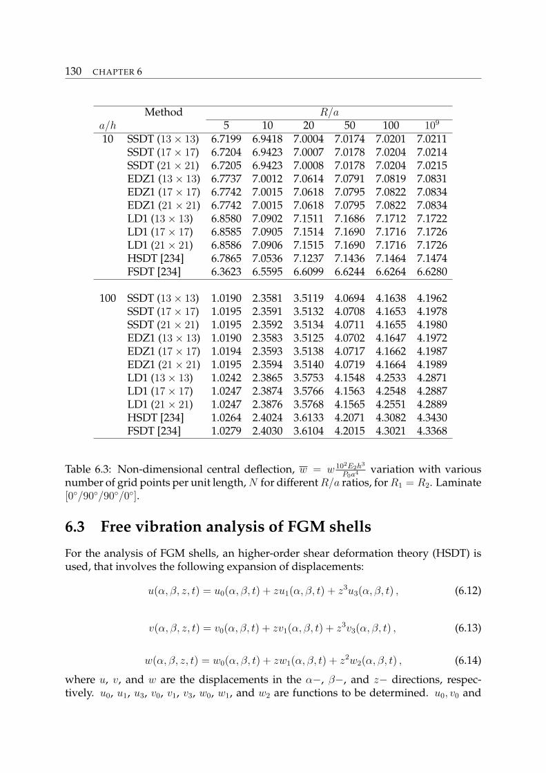
130 CHAPTER 6
Method R/aa/h 5 10 20 50 100 109
10 SSDT (13× 13) 6.7199 6.9418 7.0004 7.0174 7.0201 7.0211SSDT (17× 17) 6.7204 6.9423 7.0007 7.0178 7.0204 7.0214SSDT (21× 21) 6.7205 6.9423 7.0008 7.0178 7.0204 7.0215EDZ1 (13× 13) 6.7737 7.0012 7.0614 7.0791 7.0819 7.0831EDZ1 (17× 17) 6.7742 7.0015 7.0618 7.0795 7.0822 7.0834EDZ1 (21× 21) 6.7742 7.0015 7.0618 7.0795 7.0822 7.0834LD1 (13× 13) 6.8580 7.0902 7.1511 7.1686 7.1712 7.1722LD1 (17× 17) 6.8585 7.0905 7.1514 7.1690 7.1716 7.1726LD1 (21× 21) 6.8586 7.0906 7.1515 7.1690 7.1716 7.1726HSDT [234] 6.7865 7.0536 7.1237 7.1436 7.1464 7.1474FSDT [234] 6.3623 6.5595 6.6099 6.6244 6.6264 6.6280
100 SSDT (13× 13) 1.0190 2.3581 3.5119 4.0694 4.1638 4.1962SSDT (17× 17) 1.0195 2.3591 3.5132 4.0708 4.1653 4.1978SSDT (21× 21) 1.0195 2.3592 3.5134 4.0711 4.1655 4.1980EDZ1 (13× 13) 1.0190 2.3583 3.5125 4.0702 4.1647 4.1972EDZ1 (17× 17) 1.0194 2.3593 3.5138 4.0717 4.1662 4.1987EDZ1 (21× 21) 1.0195 2.3594 3.5140 4.0719 4.1664 4.1989LD1 (13× 13) 1.0242 2.3865 3.5753 4.1548 4.2533 4.2871LD1 (17× 17) 1.0247 2.3874 3.5766 4.1563 4.2548 4.2887LD1 (21× 21) 1.0247 2.3876 3.5768 4.1565 4.2551 4.2889HSDT [234] 1.0264 2.4024 3.6133 4.2071 4.3082 4.3430FSDT [234] 1.0279 2.4030 3.6104 4.2015 4.3021 4.3368
Table 6.3: Non-dimensional central deflection, w = w 102E2h3
P0a4 variation with variousnumber of grid points per unit length, N for different R/a ratios, for R1 = R2. Laminate[0/90/90/0].
6.3 Free vibration analysis of FGM shells
For the analysis of FGM shells, an higher-order shear deformation theory (HSDT) isused, that involves the following expansion of displacements:
u(α, β, z, t) = u0(α, β, t) + zu1(α, β, t) + z3u3(α, β, t) , (6.12)
v(α, β, z, t) = v0(α, β, t) + zv1(α, β, t) + z3v3(α, β, t) , (6.13)
w(α, β, z, t) = w0(α, β, t) + zw1(α, β, t) + z2w2(α, β, t) , (6.14)
where u, v, and w are the displacements in the α−, β−, and z− directions, respec-tively. u0, u1, u3, v0, v1, v3, w0, w1, and w2 are functions to be determined. u0, v0 and
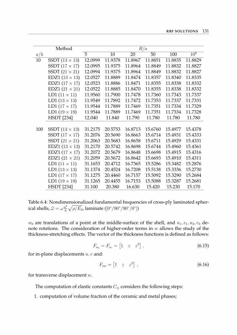
RBF SOLUTIONS 131
Method R/aa/h 5 10 20 50 100 109
10 SSDT (13× 13) 12.0999 11.9378 11.8967 11.8851 11.8835 11.8829SSDT (17× 17) 12.0995 11.9375 11.8964 11.8849 11.8832 11.8827SSDT (21× 21) 12.0994 11.9375 11.8964 11.8849 11.8832 11.8827EDZ1 (13× 13) 12.0527 11.8889 11.8474 11.8357 11.8340 11.8335EDZ1 (17× 17) 12.0523 11.8886 11.8471 11.8355 11.8338 11.8332EDZ1 (21× 21) 12.0522 11.8885 11.8470 11.8355 11.8338 11.8332LD1 (11× 11) 11.9560 11.7900 11.7478 11.7360 11.7343 11.7337LD1 (13× 13) 11.9549 11.7892 11.7472 11.7353 11.7337 11.7331LD1 (17× 17) 11.9544 11.7889 11.7469 11.7351 11.7334 11.7329LD1 (19× 19) 11.9544 11.7889 11.7469 11.7351 11.7334 11.7328HSDT [234] 12.040 11.840 11.790 11.780 11.780 11.780
100 SSDT (13× 13) 31.2175 20.5753 16.8713 15.6760 15.4977 15.4378SSDT (17× 17) 31.2076 20.5690 16.8663 15.6714 15.4931 15.4333SSDT (21× 21) 31.2063 20.5683 16.8658 15.6711 15.4929 15.4331EDZ1 (13× 13) 31.2170 20.5742 16.8698 15.6744 15.4960 15.4361EDZ1 (17× 17) 31.2072 20.5679 16.8648 15.6698 15.4915 15.4316EDZ1 (21× 21) 31.2059 20.5672 16.8642 15.6693 15.4910 15.4311LD1 (11× 11) 31.1653 20.4712 16.7365 15.5286 15.3482 15.2876LD1 (13× 13) 31.1374 20.4524 16.7208 15.5138 15.3336 15.2730LD1 (17× 17) 31.1275 20.4460 16.7157 15.5092 15.3290 15.2684LD1 (19× 19) 31.1265 20.4455 16.7153 15.5088 15.3287 15.2681HSDT [234] 31.100 20.380 16.630 15.420 15.230 15.170
Table 6.4: Nondimensionalized fundamental frequencies of cross-ply laminated spher-ical shells, ω = ω a2
h
√ρ/E2, laminate ([0/90/90/0])
w0 are translations of a point at the middle-surface of the shell, and u1, v1, u3, v3 de-note rotations. The consideration of higher-order terms in w allows the study of thethickness-stretching effects. The vector of the thickness functions is defined as follows:
Fsu = Fsv =[1 z z3
], (6.15)
for in-plane displacements u, v and:
Fsw =[1 z z2
], (6.16)
for transverse displacement w.
The computation of elastic constants Cij considers the following steps:
1. computation of volume fraction of the ceramic and metal phases;
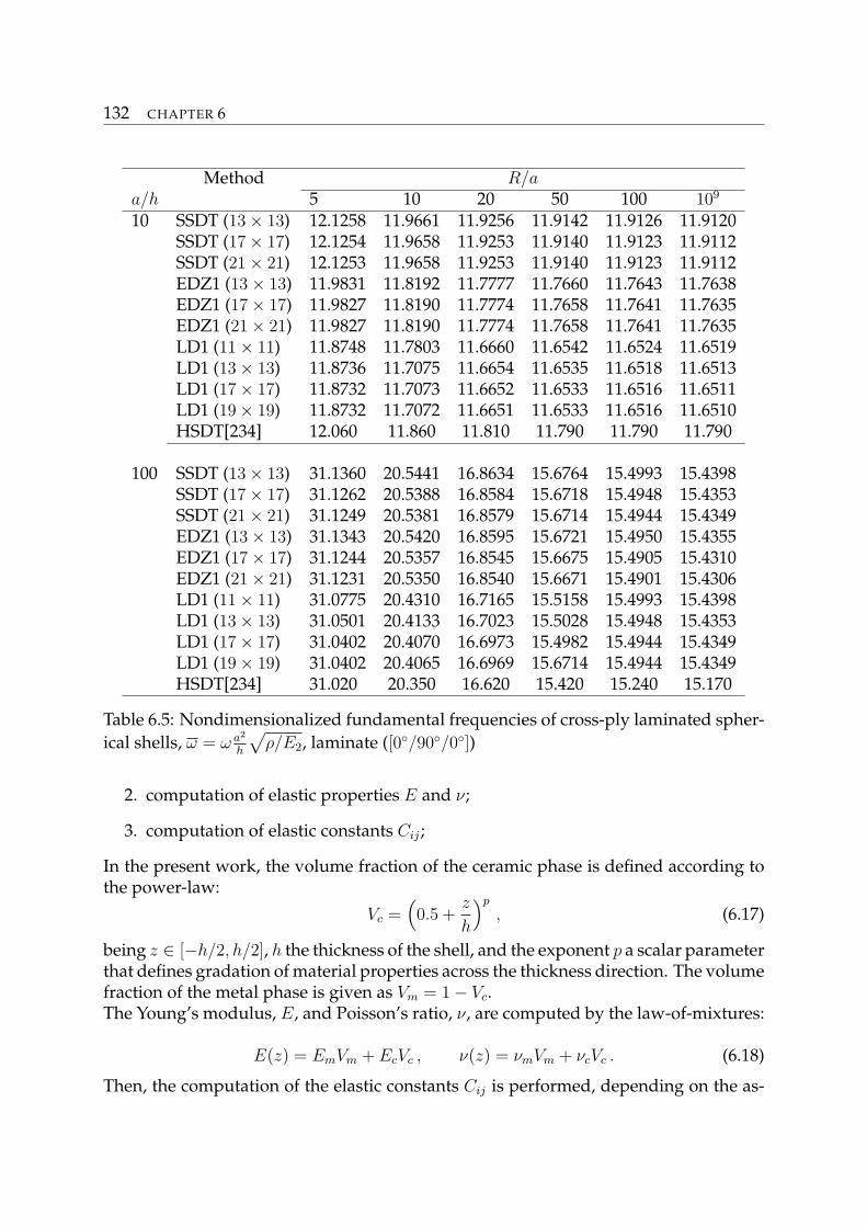
132 CHAPTER 6
Method R/aa/h 5 10 20 50 100 109
10 SSDT (13× 13) 12.1258 11.9661 11.9256 11.9142 11.9126 11.9120SSDT (17× 17) 12.1254 11.9658 11.9253 11.9140 11.9123 11.9112SSDT (21× 21) 12.1253 11.9658 11.9253 11.9140 11.9123 11.9112EDZ1 (13× 13) 11.9831 11.8192 11.7777 11.7660 11.7643 11.7638EDZ1 (17× 17) 11.9827 11.8190 11.7774 11.7658 11.7641 11.7635EDZ1 (21× 21) 11.9827 11.8190 11.7774 11.7658 11.7641 11.7635LD1 (11× 11) 11.8748 11.7803 11.6660 11.6542 11.6524 11.6519LD1 (13× 13) 11.8736 11.7075 11.6654 11.6535 11.6518 11.6513LD1 (17× 17) 11.8732 11.7073 11.6652 11.6533 11.6516 11.6511LD1 (19× 19) 11.8732 11.7072 11.6651 11.6533 11.6516 11.6510HSDT[234] 12.060 11.860 11.810 11.790 11.790 11.790
100 SSDT (13× 13) 31.1360 20.5441 16.8634 15.6764 15.4993 15.4398SSDT (17× 17) 31.1262 20.5388 16.8584 15.6718 15.4948 15.4353SSDT (21× 21) 31.1249 20.5381 16.8579 15.6714 15.4944 15.4349EDZ1 (13× 13) 31.1343 20.5420 16.8595 15.6721 15.4950 15.4355EDZ1 (17× 17) 31.1244 20.5357 16.8545 15.6675 15.4905 15.4310EDZ1 (21× 21) 31.1231 20.5350 16.8540 15.6671 15.4901 15.4306LD1 (11× 11) 31.0775 20.4310 16.7165 15.5158 15.4993 15.4398LD1 (13× 13) 31.0501 20.4133 16.7023 15.5028 15.4948 15.4353LD1 (17× 17) 31.0402 20.4070 16.6973 15.4982 15.4944 15.4349LD1 (19× 19) 31.0402 20.4065 16.6969 15.6714 15.4944 15.4349HSDT[234] 31.020 20.350 16.620 15.420 15.240 15.170
Table 6.5: Nondimensionalized fundamental frequencies of cross-ply laminated spher-ical shells, ω = ω a2
h
√ρ/E2, laminate ([0/90/0])
2. computation of elastic properties E and ν;
3. computation of elastic constants Cij ;
In the present work, the volume fraction of the ceramic phase is defined according tothe power-law:
Vc =(0.5 +
z
h
)p
, (6.17)
being z ∈ [−h/2, h/2], h the thickness of the shell, and the exponent p a scalar parameterthat defines gradation of material properties across the thickness direction. The volumefraction of the metal phase is given as Vm = 1− Vc.The Young’s modulus, E, and Poisson’s ratio, ν, are computed by the law-of-mixtures:
E(z) = EmVm + EcVc , ν(z) = νmVm + νcVc . (6.18)
Then, the computation of the elastic constants Cij is performed, depending on the as-
RBF SOLUTIONS 133
sumption of εzz. If εzz = 0, then Cij are the plane-stress reduced elastic constants:
C11 =E
1− (ν)2, C12 = ν
E
1− (ν)2, C44 =
E
2(1 + ν), C33 = 0 , (6.19)
where E is the modulus of elasticity, ν is the Poisson’s ratio found in previous step.If εzz 6= 0 (thickness-stretching), then Cij are the three-dimensional elastic constants,given by:
C11 =E(1− (ν)2)
1− 3(ν)2 − 2(ν)3, C12 =
E(ν + (ν)2)
1− 3(ν)2 − 2(ν)3, (6.20)
C44 =E
2(1 + ν), C33 =
E(1− (ν)2)
1− 3(ν)2 − 2(ν)3. (6.21)
As in Section 5.4, the material constants are directly integrated with the thickness func-tions using the Gauss integration method.
6.3.1 Results and discussion
In this section, the higher-order shear deformation theory is combined with radial basisfunctions collocation for the free vibration analysis of functionally graded shell panels.Examples include spherical (Rx = Ry = R) as well as cylindrical (Rx = R and Ry = ∞)shell panels with all edges clamped (CCCC) or simply supported (SSSS). Particularcases of these are also considered: isotropic materials (fully ceramic, p = 0, and fullymetal, p = ∞) and plates (Rx = Ry = ∞).To study the effect of εzz 6= 0 in these problems, the case εzz = 0 is implemented byconsidering w = w0 instead (6.14).Results are compared with those from Pradyumna and Bandyopadhyay [238], whoused finite elements formulation and a HSDT disregarding through-the-thickness de-formations.The following material properties are used:
silicon nitride (Si3N4):Ec = 322.2715GPa, νc = 0.24, ρc = 2370Kg/m3 , (6.22)
stainless steel (SUS304):Em = 207.7877GPa, νm = 0.31776, ρm = 8166Kg/m3 (6.23)
aluminum:Em = 70GPa, νm = 0.3, ρm = 2707Kg/m3 , (6.24)
alumina:Ec = 380GPa, νc = 0.3, ρc = 3000Kg/m3 . (6.25)
The non-dimensional frequency is given as:
w = wa2
√ρmh
D, where D =
Emh3
12(1− ν2m)
. (6.26)
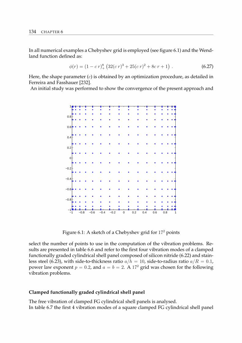
134 CHAPTER 6
In all numerical examples a Chebyshev grid is employed (see figure 6.1) and the Wend-land function defined as:
φ(r) = (1− c r)8+
(32(c r)3 + 25(c r)2 + 8c r + 1
). (6.27)
Here, the shape parameter (c) is obtained by an optimization procedure, as detailed inFerreira and Fasshauer [232].An initial study was performed to show the convergence of the present approach and
−1 −0.8 −0.6 −0.4 −0.2 0 0.2 0.4 0.6 0.8 1−1
−0.8
−0.6
−0.4
−0.2
0
0.2
0.4
0.6
0.8
1
Figure 6.1: A sketch of a Chebyshev grid for 172 points
select the number of points to use in the computation of the vibration problems. Re-sults are presented in table 6.6 and refer to the first four vibration modes of a clampedfunctionally graded cylindrical shell panel composed of silicon nitride (6.22) and stain-less steel (6.23), with side-to-thickness ratio a/h = 10, side-to-radius ratio a/R = 0.1,power law exponent p = 0.2, and a = b = 2. A 172 grid was chosen for the followingvibration problems.
Clamped functionally graded cylindrical shell panel
The free vibration of clamped FG cylindrical shell panels is analysed.In table 6.7 the first 4 vibration modes of a square clamped FG cylindrical shell panel
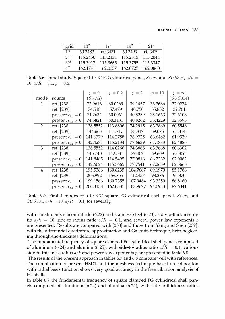
RBF SOLUTIONS 135
grid 132 172 192 212
1st 60.3483 60.3431 60.3499 60.34792nd 115.2450 115.2134 115.2315 115.20443rd 115.3917 115.3665 115.3755 115.33474th 162.1741 162.0337 162.0727 162.0860
Table 6.6: Initial study. Square CCCC FG cylindrical panel, Si3N4 and SUS304, a/h =10, a/R = 0.1, p = 0.2.
p = 0 p = 0.2 p = 2 p = 10 p = ∞mode source (Si3N4) (SUS304)
1 ref. [238] 72.9613 60.0269 39.1457 33.3666 32.0274ref. [239] 74.518 57.479 40.750 35.852 32.761present εzz = 0 74.2634 60.0061 40.5259 35.1663 32.6108present εzz 6= 0 74.5821 60.3431 40.8262 35.4229 32.8593
2 ref. [238] 138.5552 113.8806 74.2915 63.2869 60.5546ref. [239] 144.663 111.717 78.817 69.075 63.314present εzz = 0 141.6779 114.3788 76.9725 66.6482 61.9329present εzz 6= 0 142.4281 115.2134 77.6639 67.1883 62.4886
3 ref. [238] 138.5552 114.0266 74.3868 63.3668 60.6302ref. [239] 145.740 112.531 79.407 69.609 63.806present εzz = 0 141.8485 114.5495 77.0818 66.7332 62.0082present εzz 6= 0 142.6024 115.3665 77.7541 67.2689 62.5668
4 ref. [238] 195.5366 160.6235 104.7687 89.1970 85.1788ref. [239] 206.992 159.855 112.457 98.386 90.370present εzz = 0 199.1566 160.7355 107.9484 93.3350 86.8160present εzz 6= 0 200.3158 162.0337 108.9677 94.0923 87.6341
Table 6.7: First 4 modes of a CCCC square FG cylindrical shell panel, Si3N4 andSUS304, a/h = 10, a/R = 0.1, for several p.
with constituents silicon nitride (6.22) and stainless steel (6.23), side-to-thickness ra-tio a/h = 10, side-to-radius ratio a/R = 0.1, and several power law exponents pare presented. Results are compared with [238] and those from Yang and Shen [239],with the differential quadrature approximation and Galerkin technique, both neglect-ing through-the-thickness deformations.The fundamental frequency of square clamped FG cylindrical shell panels composed
of aluminum (6.24) and alumina (6.25), with side-to-radius ratio a/R = 0.1, variousside-to-thickness ratios a/h and power law exponents p are presented in table 6.8.The results of the present approach in tables 6.7 and 6.8 compare well with references.
The combination of present HSDT and the meshless technique based on collocationwith radial basis function shows very good accuracy in the free vibration analysis ofFG shells.In table 6.9 the fundamental frequency of square clamped FG cylindrical shell pan-els composed of aluminum (6.24) and alumina (6.25), with side-to-thickness ratios
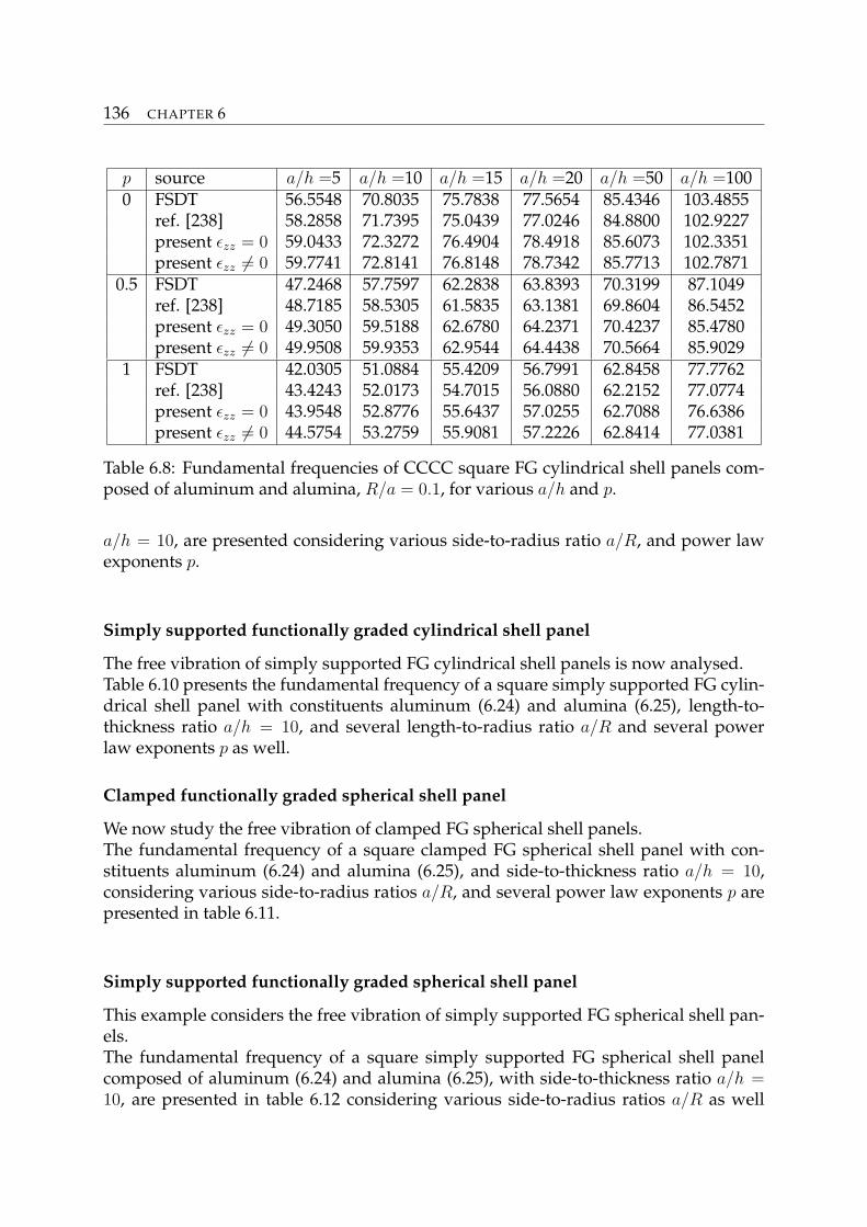
136 CHAPTER 6
p source a/h =5 a/h =10 a/h =15 a/h =20 a/h =50 a/h =1000 FSDT 56.5548 70.8035 75.7838 77.5654 85.4346 103.4855
ref. [238] 58.2858 71.7395 75.0439 77.0246 84.8800 102.9227present εzz = 0 59.0433 72.3272 76.4904 78.4918 85.6073 102.3351present εzz 6= 0 59.7741 72.8141 76.8148 78.7342 85.7713 102.7871
0.5 FSDT 47.2468 57.7597 62.2838 63.8393 70.3199 87.1049ref. [238] 48.7185 58.5305 61.5835 63.1381 69.8604 86.5452present εzz = 0 49.3050 59.5188 62.6780 64.2371 70.4237 85.4780present εzz 6= 0 49.9508 59.9353 62.9544 64.4438 70.5664 85.9029
1 FSDT 42.0305 51.0884 55.4209 56.7991 62.8458 77.7762ref. [238] 43.4243 52.0173 54.7015 56.0880 62.2152 77.0774present εzz = 0 43.9548 52.8776 55.6437 57.0255 62.7088 76.6386present εzz 6= 0 44.5754 53.2759 55.9081 57.2226 62.8414 77.0381
Table 6.8: Fundamental frequencies of CCCC square FG cylindrical shell panels com-posed of aluminum and alumina, R/a = 0.1, for various a/h and p.
a/h = 10, are presented considering various side-to-radius ratio a/R, and power lawexponents p.
Simply supported functionally graded cylindrical shell panel
The free vibration of simply supported FG cylindrical shell panels is now analysed.Table 6.10 presents the fundamental frequency of a square simply supported FG cylin-drical shell panel with constituents aluminum (6.24) and alumina (6.25), length-to-thickness ratio a/h = 10, and several length-to-radius ratio a/R and several powerlaw exponents p as well.
Clamped functionally graded spherical shell panel
We now study the free vibration of clamped FG spherical shell panels.The fundamental frequency of a square clamped FG spherical shell panel with con-stituents aluminum (6.24) and alumina (6.25), and side-to-thickness ratio a/h = 10,considering various side-to-radius ratios a/R, and several power law exponents p arepresented in table 6.11.
Simply supported functionally graded spherical shell panel
This example considers the free vibration of simply supported FG spherical shell pan-els.The fundamental frequency of a square simply supported FG spherical shell panelcomposed of aluminum (6.24) and alumina (6.25), with side-to-thickness ratio a/h =10, are presented in table 6.12 considering various side-to-radius ratios a/R as well
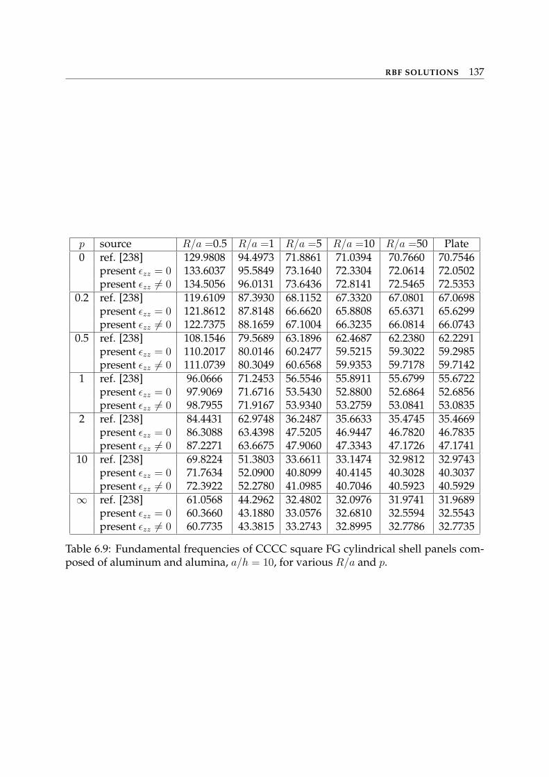
RBF SOLUTIONS 137
p source R/a =0.5 R/a =1 R/a =5 R/a =10 R/a =50 Plate0 ref. [238] 129.9808 94.4973 71.8861 71.0394 70.7660 70.7546
present εzz = 0 133.6037 95.5849 73.1640 72.3304 72.0614 72.0502present εzz 6= 0 134.5056 96.0131 73.6436 72.8141 72.5465 72.5353
0.2 ref. [238] 119.6109 87.3930 68.1152 67.3320 67.0801 67.0698present εzz = 0 121.8612 87.8148 66.6620 65.8808 65.6371 65.6299present εzz 6= 0 122.7375 88.1659 67.1004 66.3235 66.0814 66.0743
0.5 ref. [238] 108.1546 79.5689 63.1896 62.4687 62.2380 62.2291present εzz = 0 110.2017 80.0146 60.2477 59.5215 59.3022 59.2985present εzz 6= 0 111.0739 80.3049 60.6568 59.9353 59.7178 59.7142
1 ref. [238] 96.0666 71.2453 56.5546 55.8911 55.6799 55.6722present εzz = 0 97.9069 71.6716 53.5430 52.8800 52.6864 52.6856present εzz 6= 0 98.7955 71.9167 53.9340 53.2759 53.0841 53.0835
2 ref. [238] 84.4431 62.9748 36.2487 35.6633 35.4745 35.4669present εzz = 0 86.3088 63.4398 47.5205 46.9447 46.7820 46.7835present εzz 6= 0 87.2271 63.6675 47.9060 47.3343 47.1726 47.1741
10 ref. [238] 69.8224 51.3803 33.6611 33.1474 32.9812 32.9743present εzz = 0 71.7634 52.0900 40.8099 40.4145 40.3028 40.3037present εzz 6= 0 72.3922 52.2780 41.0985 40.7046 40.5923 40.5929
∞ ref. [238] 61.0568 44.2962 32.4802 32.0976 31.9741 31.9689present εzz = 0 60.3660 43.1880 33.0576 32.6810 32.5594 32.5543present εzz 6= 0 60.7735 43.3815 33.2743 32.8995 32.7786 32.7735
Table 6.9: Fundamental frequencies of CCCC square FG cylindrical shell panels com-posed of aluminum and alumina, a/h = 10, for various R/a and p.
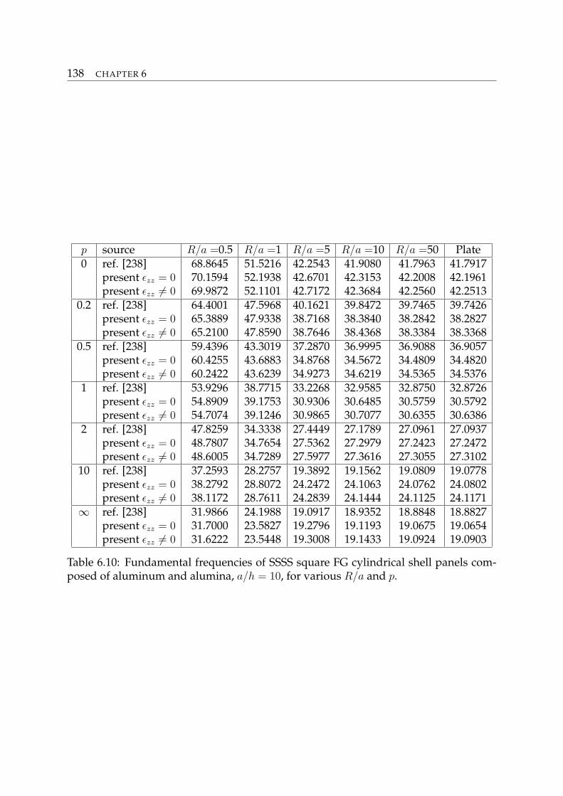
138 CHAPTER 6
p source R/a =0.5 R/a =1 R/a =5 R/a =10 R/a =50 Plate0 ref. [238] 68.8645 51.5216 42.2543 41.9080 41.7963 41.7917
present εzz = 0 70.1594 52.1938 42.6701 42.3153 42.2008 42.1961present εzz 6= 0 69.9872 52.1101 42.7172 42.3684 42.2560 42.2513
0.2 ref. [238] 64.4001 47.5968 40.1621 39.8472 39.7465 39.7426present εzz = 0 65.3889 47.9338 38.7168 38.3840 38.2842 38.2827present εzz 6= 0 65.2100 47.8590 38.7646 38.4368 38.3384 38.3368
0.5 ref. [238] 59.4396 43.3019 37.2870 36.9995 36.9088 36.9057present εzz = 0 60.4255 43.6883 34.8768 34.5672 34.4809 34.4820present εzz 6= 0 60.2422 43.6239 34.9273 34.6219 34.5365 34.5376
1 ref. [238] 53.9296 38.7715 33.2268 32.9585 32.8750 32.8726present εzz = 0 54.8909 39.1753 30.9306 30.6485 30.5759 30.5792present εzz 6= 0 54.7074 39.1246 30.9865 30.7077 30.6355 30.6386
2 ref. [238] 47.8259 34.3338 27.4449 27.1789 27.0961 27.0937present εzz = 0 48.7807 34.7654 27.5362 27.2979 27.2423 27.2472present εzz 6= 0 48.6005 34.7289 27.5977 27.3616 27.3055 27.3102
10 ref. [238] 37.2593 28.2757 19.3892 19.1562 19.0809 19.0778present εzz = 0 38.2792 28.8072 24.2472 24.1063 24.0762 24.0802present εzz 6= 0 38.1172 28.7611 24.2839 24.1444 24.1125 24.1171
∞ ref. [238] 31.9866 24.1988 19.0917 18.9352 18.8848 18.8827present εzz = 0 31.7000 23.5827 19.2796 19.1193 19.0675 19.0654present εzz 6= 0 31.6222 23.5448 19.3008 19.1433 19.0924 19.0903
Table 6.10: Fundamental frequencies of SSSS square FG cylindrical shell panels com-posed of aluminum and alumina, a/h = 10, for various R/a and p.
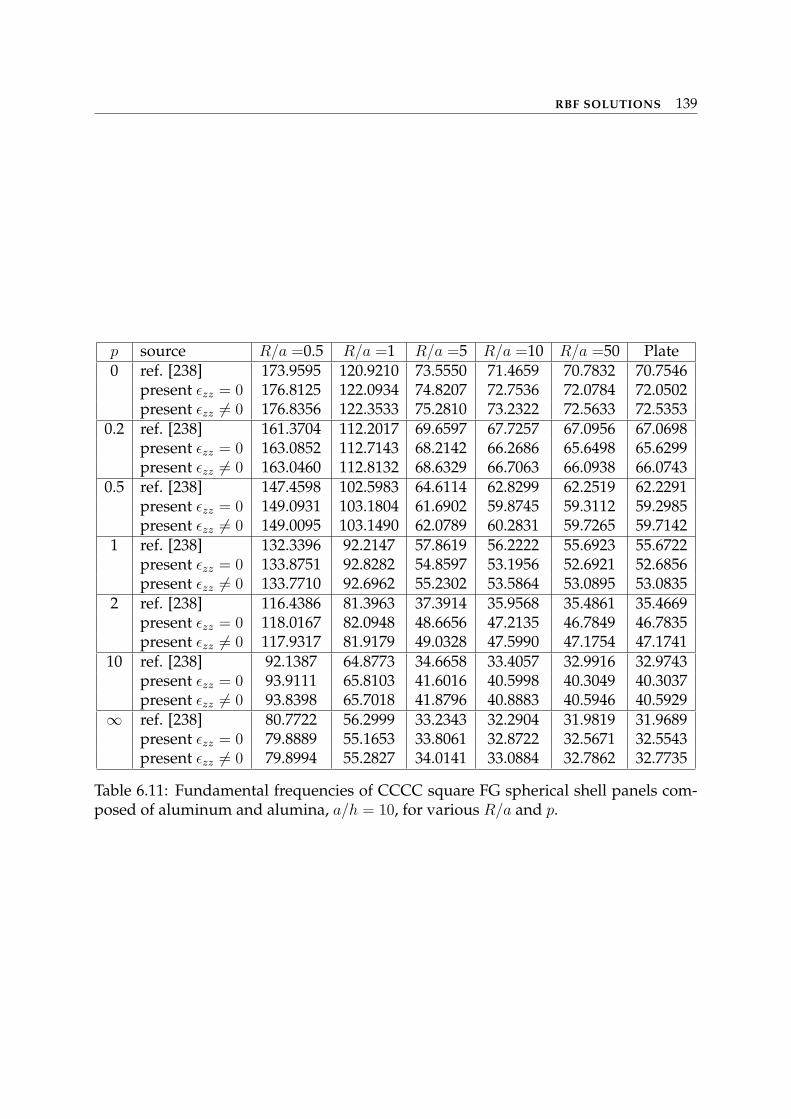
RBF SOLUTIONS 139
p source R/a =0.5 R/a =1 R/a =5 R/a =10 R/a =50 Plate0 ref. [238] 173.9595 120.9210 73.5550 71.4659 70.7832 70.7546
present εzz = 0 176.8125 122.0934 74.8207 72.7536 72.0784 72.0502present εzz 6= 0 176.8356 122.3533 75.2810 73.2322 72.5633 72.5353
0.2 ref. [238] 161.3704 112.2017 69.6597 67.7257 67.0956 67.0698present εzz = 0 163.0852 112.7143 68.2142 66.2686 65.6498 65.6299present εzz 6= 0 163.0460 112.8132 68.6329 66.7063 66.0938 66.0743
0.5 ref. [238] 147.4598 102.5983 64.6114 62.8299 62.2519 62.2291present εzz = 0 149.0931 103.1804 61.6902 59.8745 59.3112 59.2985present εzz 6= 0 149.0095 103.1490 62.0789 60.2831 59.7265 59.7142
1 ref. [238] 132.3396 92.2147 57.8619 56.2222 55.6923 55.6722present εzz = 0 133.8751 92.8282 54.8597 53.1956 52.6921 52.6856present εzz 6= 0 133.7710 92.6962 55.2302 53.5864 53.0895 53.0835
2 ref. [238] 116.4386 81.3963 37.3914 35.9568 35.4861 35.4669present εzz = 0 118.0167 82.0948 48.6656 47.2135 46.7849 46.7835present εzz 6= 0 117.9317 81.9179 49.0328 47.5990 47.1754 47.1741
10 ref. [238] 92.1387 64.8773 34.6658 33.4057 32.9916 32.9743present εzz = 0 93.9111 65.8103 41.6016 40.5998 40.3049 40.3037present εzz 6= 0 93.8398 65.7018 41.8796 40.8883 40.5946 40.5929
∞ ref. [238] 80.7722 56.2999 33.2343 32.2904 31.9819 31.9689present εzz = 0 79.8889 55.1653 33.8061 32.8722 32.5671 32.5543present εzz 6= 0 79.8994 55.2827 34.0141 33.0884 32.7862 32.7735
Table 6.11: Fundamental frequencies of CCCC square FG spherical shell panels com-posed of aluminum and alumina, a/h = 10, for various R/a and p.
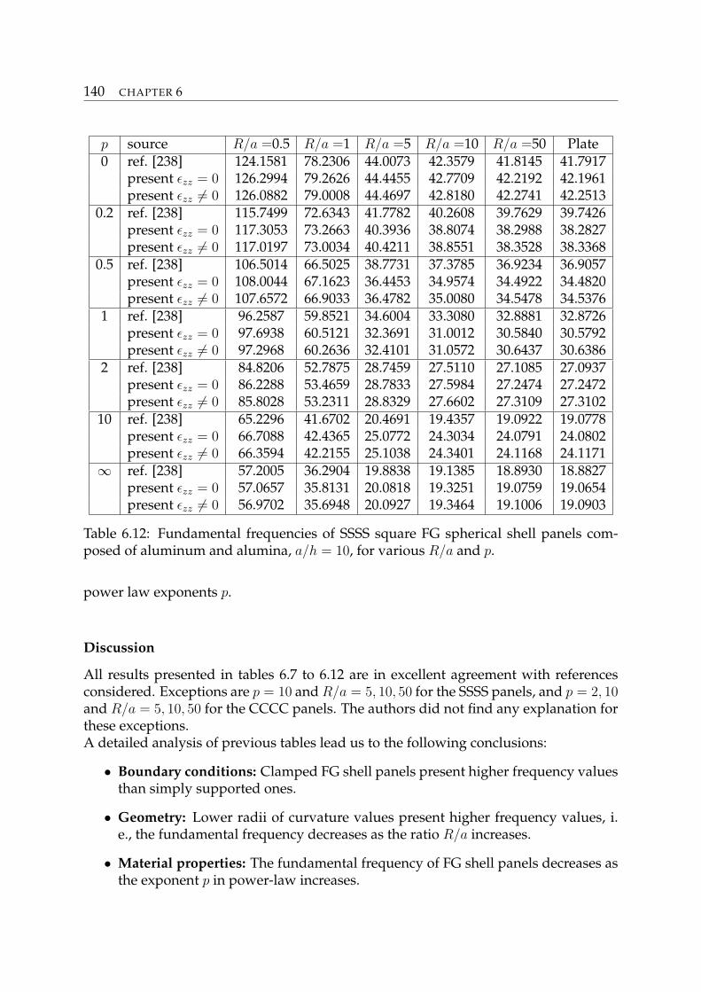
140 CHAPTER 6
p source R/a =0.5 R/a =1 R/a =5 R/a =10 R/a =50 Plate0 ref. [238] 124.1581 78.2306 44.0073 42.3579 41.8145 41.7917
present εzz = 0 126.2994 79.2626 44.4455 42.7709 42.2192 42.1961present εzz 6= 0 126.0882 79.0008 44.4697 42.8180 42.2741 42.2513
0.2 ref. [238] 115.7499 72.6343 41.7782 40.2608 39.7629 39.7426present εzz = 0 117.3053 73.2663 40.3936 38.8074 38.2988 38.2827present εzz 6= 0 117.0197 73.0034 40.4211 38.8551 38.3528 38.3368
0.5 ref. [238] 106.5014 66.5025 38.7731 37.3785 36.9234 36.9057present εzz = 0 108.0044 67.1623 36.4453 34.9574 34.4922 34.4820present εzz 6= 0 107.6572 66.9033 36.4782 35.0080 34.5478 34.5376
1 ref. [238] 96.2587 59.8521 34.6004 33.3080 32.8881 32.8726present εzz = 0 97.6938 60.5121 32.3691 31.0012 30.5840 30.5792present εzz 6= 0 97.2968 60.2636 32.4101 31.0572 30.6437 30.6386
2 ref. [238] 84.8206 52.7875 28.7459 27.5110 27.1085 27.0937present εzz = 0 86.2288 53.4659 28.7833 27.5984 27.2474 27.2472present εzz 6= 0 85.8028 53.2311 28.8329 27.6602 27.3109 27.3102
10 ref. [238] 65.2296 41.6702 20.4691 19.4357 19.0922 19.0778present εzz = 0 66.7088 42.4365 25.0772 24.3034 24.0791 24.0802present εzz 6= 0 66.3594 42.2155 25.1038 24.3401 24.1168 24.1171
∞ ref. [238] 57.2005 36.2904 19.8838 19.1385 18.8930 18.8827present εzz = 0 57.0657 35.8131 20.0818 19.3251 19.0759 19.0654present εzz 6= 0 56.9702 35.6948 20.0927 19.3464 19.1006 19.0903
Table 6.12: Fundamental frequencies of SSSS square FG spherical shell panels com-posed of aluminum and alumina, a/h = 10, for various R/a and p.
power law exponents p.
Discussion
All results presented in tables 6.7 to 6.12 are in excellent agreement with referencesconsidered. Exceptions are p = 10 and R/a = 5, 10, 50 for the SSSS panels, and p = 2, 10and R/a = 5, 10, 50 for the CCCC panels. The authors did not find any explanation forthese exceptions.A detailed analysis of previous tables lead us to the following conclusions:
• Boundary conditions: Clamped FG shell panels present higher frequency valuesthan simply supported ones.
• Geometry: Lower radii of curvature values present higher frequency values, i.e., the fundamental frequency decreases as the ratio R/a increases.
• Material properties: The fundamental frequency of FG shell panels decreases asthe exponent p in power-law increases.

RBF SOLUTIONS 141
Another conclusion from all tables is that the fundamental frequency decreases as theradius of curvature increases. The fall-off is faster for smaller values of R (R/a) andthen shows fast convergence.The effect of εzz 6= 0 shows significance in thicker shells (see table 6.7) and seems inde-pendent of the radius of curvature (see tables 6.9 to 6.12 ).

Chapter 7
Conclusions
The analysis of advanced structures involved in multi-field problems has been con-sidered in this thesis. In particular, the analysis of composite shells, the thermal andmechanical analysis of FGM shells, the electromechanical analysis of shell structuresembedding piezoelectric layers and the analysis of carbon nanotubes have been per-formed.The shell models contained in the CUF have been used to model the field variables: dis-placements, temperature, electrical potential, transverse stress components and nor-mal electrical displacement (in the case of FGM structures, the CUF can be used also tomodel the material properties). These models differ in the variable description (Equiv-alent Single Layer (ESL) or Layer Wise (LW)) and in the order of expansion in the thick-ness direction used for the primary variables of the problem. Moreover, refined or ad-vanced models can be considered in the CUF, depending on the variational statementemployed for the derivation of governing equations. The refined models are developedin the framework of the Principle of Virtual Displacements (PVD) with the possibilityof a priori modelling the displacements, the electric potential and the temperature.The advanced models, also called mixed models, are developed in the framework ofReissner’s Mixed Variational Theorem (RMVT), which permits the displacements, theelectric potential, the temperature, the transverse shear/normal stresses and the trans-verse normal electric displacement, to be considered as independent variables. Theobtained governing equations have been solved in analytical way using the Naviermethod or in numerical way, using the Finite Element Method and the Radial BasisFunctions method. In particular, this last is a meshless method recently proposed toovercome the numerical problems of the finite element method relative to the mesh.Note that, the cases of FEM and RBF methods combined with the Unified Formulationand shell geometries is a new approach that has been firstly introduced in this thesis.
The main results have been organized in three parts: the analytical solutions ob-tained using the Navier method, the solutions obtained by means of the FEM and thesolutions calculated with the RBF method.
In the first part, an extension of the Carrera’s Unified Formulation which accounts
143
144 CHAPTER 7
for functionally graded shells subjected to thermal loads has been presented. It hasbeen shown that the unified treatment of all the considered variables (displacements,temperature, material) can include any kind of material gradient. The CUF providesvery accurate results, compared to reference solutions, although the use of higher or-der expansions in the thickness direction are mandatory. It has been found that thetemperature profile cannot be assumed linear in an FGM layer, even when a very thinshell is considered. The assumption of a constant transverse deflection through thethickness direction is not valid in the thermal case; lower errors are produced in thecase of the mechanical loading. The influence of material gradient is more significantfor a thermal loading than for mechanical loadings.Then, the electromechanical problem has been analyzed using both the Principle of Vir-tual Displacements and Reissner’s Mixed Variational Theorem. In particular, variousforms of RMVT have been discussed in which the transverse shear/normal stressesand/or the transverse normal electric displacement are a priori modelled. The gov-erning differential equations are derived according to Carrera’s Unified Formulationfor multilayered shells and the closed-form solutions of the free vibration problemof simply supported, orthotropic piezoelectric laminates in closed circuit configura-tions (electric potential imposed to zero at the top and bottom) have been calculated.The frequencies obtained from the free vibrations analysis of a multilayered ring shellhave been compared with the three-dimensional solution and the following conclu-sions have been drawn:
1. The use of Layer Wise models is mandatory to achieve a 3D solution, whereasEquivalent Single Layer models give erroneous results even when higher ordersof expansion are used; classical theories such as CLT and FSDT could lead tolarge errors.
2. Mixed theories do not significantly improve the results in terms of circular fre-quency parameters; however, their use becomes mandatory to predict the correct’through the thickness’ modes for both transverse mechanical and electrical vari-ables.
3. The effect produced by the electromechanical interaction on the frequency re-sponse approximately increases with the thickness ratio of the shell but decreaseswith the wave numbers m and n. However this effect depends no more on wavenumber when the shell is very thin.
Finally, the refined shell models contained in the Unified Formulation have been ap-plied to the study of the dynamic response in double-walled carbon nanotubes. TheDWNT was assumed to be an equivalent continuum cylindrical shell made up of twolayers and both ESL and LW models have been employed in the analysis. In particular,the LW models have been modified in order to consider two DWNT tubes as sepa-rately vibrating and to account for the van der Waals interaction between them. Thefollowing conclusions have been made:
• refined shell models can successfully be extended to the free vibration analysis of
CONCLUSIONS 145
DWNTs and they give a satisfactory analysis for both long and short CNTs, forboth lower and higher frequencies;
• the introduction of the van der Waals forces makes it possible to consider twoadjacent tubes and leads to lower frequency values;
• the introduction of the vdW forces is mandatory for short CNTs and/or higherfrequencies.
The second part of this thesis is dedicated to the FEM analysis of composite andFGM shells. The governing equations are derived from the PVD for the pure-mechanicalproblem. Firstly, an assessment of the shell finite element based on the CUF has beenpresented. In this element, the Mixed Interpolation of Tensorial Components methodhas been employed to contrast the membrane and shear locking phenomenon. Theresults obtained by analyzing two classical test problems, such as pinched shell andScordelis-Lo problem, have shown that:
• The MITC9 shell element presents good properties of convergence and robust-ness;
• The MITC method remains effective in the case of shell FEs formulated on thebasis of higher-order theories contained in the Unified Formulation;
• The MITC9 element is completely locking free.
Then, the static analysis of cylindrical composite structures has been performed. Theresults have been provided in terms of both displacement, in plane stresses and trans-verse stresses, for various thickness ratios from very thick to very thin shells. Theperformances of the shell element have been tested and the different theories (classicaland refined) contained in the CUF have been compared. The conclusions that can bedrawn are the following:
1. the shell element is completely locking free, even when the shell is very thin;
2. the results converge to the exact solution by increasing the number of the ele-ments and the order of expansion of the displacements in the thickness direction;
3. when the shell is very thick, the LW models work better than ZZ ones, and theselast work better than ESL models;
4. the classical models, such as CLT and FSDT completely fail in the analysis of thickshells;
5. the use of LW models is mandatory for both thick and thin shells, if one needs toaccurately describe the distribution of trasverse stresses in the thickness and tosatisfy the interlaminar continuity conditions.
146 CHAPTER 7
Finally, the CUF shell finite element has been used for the mechanical analysis of FGMshells and the grading material variation in the thickness direction has been taken intoaccount. The shell considered is simply supported and subjected to a bi-sinusoidalpressure load. These conditions permit to calculate the quasi-3D analytical solution ofthe problem by means of the Navier method and higher-order models. The compar-ison of the FEM results with the quasi-3D solution has shown that the shell elementprovides very accurate results. The locking phenomenon does’t appear, even if theconsidered structure is very thin. The use of higher-order expansions is necessary tocorrectly describe the distribution of displacements and stresses along the thicknessin functionally graded shells. Moreover, it has been confirmed that the assumption ofconstant transversal displacement, on which the FSDT is based, is not valid in FGMs.
The Radial Basis Functions method has been used in the last part of this thesis. Asinusoidal shear deformation theory (SSDT), EDZ1 and LD1 models have been imple-mented for the analysis of laminated orthotropic elastic shells through a multiquadricsdiscretization of equations of motion and boundary conditions. Firstly, an assessmentof the RBF method has been presented for the plate case. The results have been com-pared with the analytical solution and the FEM results obtained with two differentshell finite elements: MITC4 and MITC9 based on the CUF. In both cases, the RBFmethod was in good agreement with the reference solution. Then, the solutions ofboth shell bending and free vibration problem have been presented. The results havebeen provided in terms of static deformations and natural frequencies and they havebeen compared with other sources. The present meshless approach demonstrated thatis very successful in the analysis of laminated composite shells. Advantages of radialbasis functions are absence of mesh, ease of discretization of boundary conditions andequations of equilibrium or motion and very easy coding. The static displacementsand the natural frequencies obtained have been shown to be in excellent agreementwith analytical solutions.Finally, the Carrera’s Unified Formulation have been combined with the Radial BasisFunctions collocation technique for the free vibration analysis of functionally gradedshells. A higher-order shear deformation theory that allows extensibility in the thick-ness direction have been implemented and the effect of εzz 6= 0 have been studied. Nu-merical results have been compared with other sources and also in this case the presentapproach demonstrated to be successful in the free vibration analysis of functionallygraded shells and easy to implement.
7.1 Outlooks
The first objective of the future work is the implementation of an isoparametric shellelement based on the CUF, that permits to analyze structures with arbitrary geometry.Similarly to the geometrically exact shell element presented in this thesis, the geometri-cal relations are derived from the Green-Lagrange strain tensor (Eq.(2.8)), consideringthe following approximations by means of Lagrangian shape functions for both the
CONCLUSIONS 147
displacement and the position vector:
u = Niui , R = NiRi , (7.1)
with i = 1, .., 9. The vectors u and R contains the displacement components and thecoordinates of a generic point in the volume of the shell, respectively, expressed inthe cartesian reference system (x, y, z). Therefore, the geometry of the shell is approxi-mated by knowing the position vector of the nodes of the element.In order to derive the geometrical relations, it is necessary also to define a unique nor-mal vector to the surface, called director field D, in each node of the element. As theposition vector, the director field is interpolated on the nodes by means of the shapefunctions:
D = NiDi . (7.2)
The MITC method will be applied to contrast the membrane and shear locking phe-nomenon as shown in Section 3.3.1.Another objective is to extend the present shell finite element to the mixed models con-tained in the CUF. In this case, the use of the RMTV permits not only to fulfil the C0
z
requirements for the transverse stresses, but also to contrast the locking. Indeed, fol-lowing the same strategy of the MITC method, the stresses, that are modelled a priori,can be opportunely interpolated in the domain of the element using points that aredifferent from the interpolation points of the displacements.The analysis of the results presented in Chapter 4 has demonstrated the superiority ofthe refined and advanced shell models contained in the CUF in the study of multi-fieldproblems. For these reasons, it is reasonable to extend the present shell element to thethermo-mechanical analysis of FGM structures and the electromechanical analysis ofpiezoelectric shells in order to overcome the limits of classical shell elements proposedin literature.At the same time, also the RBF method, that is a good alternative to the FEM, will beextended to mixed formulations and multi-field problems.

Conclusioni
In questa tesi è stata considerata l’analisi di strutture avanzate coinvolte in problemi multicampo. I modelli guscio contenuti nella CUF sono stati utilizzati per modellare le diversevariabili di campo (spostamenti, temperatura, potenziale elettrico, tensioni trasversali e sposta-mento elettrico normale). Le equazioni di governo sono state risolte sia analiticamente, tramiteil metodo di Navier, che numericamente, usando il metodo degli elementi finiti (FEM) e ilmetodo delle collocazioni tramite radial basis functions (RBF) . I risultati ottenuti sono statiorganizzati in tre parti: soluzioni analitiche, soluzioni FEM e soluzioni RBF.
Nella prima parte, è stata presentata l’analisi di gusci FGM soggetti a carichi termici emeccanici. E’ stato dimostrato che il profilo di temperatura lungo lo spessore non può essereconsiderato lineare in uno strato FGM, anche quando il guscio è molto sottile. Di conseguenza,lo spostamento trasversale non può essere assunto costante lungo lo spessore, come si ritrovanelle teorie classiche. Questo è vero anche nei gusci FGM soggetti a carico meccanico puro,anche se in maniera meno evidente. Successivamente, è stato analizzato il problema elettromec-canico in strutture contenenti strati in materiale piezoelettrico. I modelli misti basati sul prin-cipio variazionale RMVT sono stati utilizzati per l’analisi. Principalmente, si è visto che l’usodei modelli misti è necessario per descrivere correttamente l’andamento lungo lo spessore dellevariabili trasversali sia meccaniche (tensioni trasversali) che elettriche (spostamento elettriconormale). Infine, è stata effettuata l’analisi dinamica di un double-walled carbon nanotubetramite i modelli LW contenuti nella CUF, che permettono di tener conto delle forze di Van derWaals che agiscono tra le due pareti. I risultati hanno mostrato una buona concordanza con lasoluzione di riferimento data in letteratura.
La seconda parte della tesi è dedicata all’analisi meccanica di strutture guscio tramite l’elementofinito basato sulla CUF. Innanzitutto, è stato verificato che l’elemento finito fosse libero dalfenomeno del loking. E’ stata effettuata l’analisi di alcuni problemi discriminanti presi dallaletteratura che riguardano gusci isotropi molto sottili ed è stato dimostrato che l’elemento pre-senta buone proprietà di convergenza numerica. Successivamente, sono stati presentati i risul-tati ottenuti dall’analisi di gusci in materiale composito ed è stata evidenziata l’importanzadi utilizzare i modelli LW per descrivere correttamente l’andamento delle tensioni trasversalilungo lo spessore del guscio. Infine, sono stati analizzati gusci FGM e sono state confermate leconclusioni viste con il metodo analitico.
Nell’ultima parte della tesi il metodo RBF è stato utilizzato per l’analisi di gusci in materialecomposito e FGM. I risultati ottenuti sono stati comparati con i risultati analitici e i risultatiFEM ed è stato provato che il metodo funziona molto bene. In pratica, e’ stato dimostrato chel’utilizzo del metodo RBF è vantaggioso rispetto al FEM perché non presenta problemi numericilegati alla mesh, quali il locking, e la discretizzazione e l’implementazione delle equazioni di

150 CHAPTER 7
governo risultano molto semplici.
Conclusions
Dans cette thèse, on a considéré l’analyse de structures avancées dans un cadre multi-physique.Les modèles coques dérivés de la CUF ont été utilisés pour modéliser les différentes variables duchamp (déplacement, température, potentiel électrique, contraintes transversales et déplace-ment électrique normal). Les équations fondamentales ont été résolues analytiquement aumoyen de la méthode de Navier, et numériquement, en utilisant la méthode des éléments fi-nis (FEM) et la méthode sans maillage utilisant des fonctions de base radiale (RBF).
Les résultats obtenus ont été organisés en trois parties: solutions analytiques, solutionsFEM et solutions RBF. Dans la première partie on a présenté l’analyse des coques FGM soumisesà des chargements thermiques et mécaniques. On a démontré que le profil de température le longde l’épaisseur ne peut pas être considéré comme linéaire pour une coque FGM, même quand lacoque est très mince. En conséquence le déplacement transversale ne peut être supposé constantle long de l’épaisseur, comme dans les théories classiques. C’est aussi vrai pour les coques FGMsoumises à des chargements mécaniques pures. Ensuite, des problèmes électromécaniques ontété traités pour des coques piézo-électrique. Les modèles mixtes, basés sur le principe variation-nel RMVT, ont été utilisés. On a observé que l’utilisation des modèles mixtes est nécessairespour décrire correctement la distribution le long de l’épaisseur des contraintes transversales etdu déplacement électrique. Enfin, l’analyse dynamique d’un carbon nanotube à double paroien utilisant les modèles LW de la CUF a été présenté. Cela permet de tenir compte des forcesde Van der Waals qui agissent entre les deux parois. Les résultats ont démontré une bonneadéquation avec les solutions de référence de la littérature.
La deuxième partie a été consacrée à l’analyse mécanique des structures coques au moyend’un nouvel élément fini utilisant la CUF. Cet EF n’est pas sensible au phénomène de ver-rouillage. On a réalisé l’analyse de certains problèmes discriminants trouvés dans la littératureet qui concernent les coques isotropes très minces. Cette analyse a permis de démontrer quecet EF présente de bonnes propriétés de convergence numérique. Des tests concernant des co-ques en matériaux composites ont ensuite été présentés. Cela a permis de mette en évidencel’importance de l’utilisation des modèles LW pour décrire correctement la distribution des con-traintes transversales à travers la coque. Les coques FGM ont enfin été analysées permettantde confirmer les conclusions observées en utilisant la méthode analytique.
Dans la dernière partie, la méthode RBF a été utilisée pour l’analyse des coques compositeet FGM. Les résultats obtenus ont été comparés avec les résultats analytiques et FEM. On a puconstaté que la méthode fonctionnait parfaitement. L’utilisation de la méthode RBF présente lesavantages des méthodes sans maillage par rapport à la FEM. De plus, l’obtention des équationsfondamentales est assez simple.

Bibliography
[1] PANTELAKIS, SP.G., ALEXOPOULOS, N.D., Assessment of the ability of conventionaland advanced wrought aluminum alloys for mechanical performance in light-weight ap-plications, Materials & Design, 29(1), 80-91, 2008.
[2] REDDY, J.N., Mechanics of Laminated Composite Plates and Shells. Theory andAnalysis, CRC Press, 2004, New York (USA).
[3] JONES, R.M., Mechanics of Composite Materials, Second Edition, Taylor & Fran-cis, 1999, PA (USA).
[4] GIBSON, R.F., Principle of Composite Material Mechanics, McGraw-Hill, 1994,New York (USA).
[5] CHEN, A., DAVALOS, J.F., A solution including skin effect for stiffness and stress fieldof sandwich honeycombe core, International Journal of Solids and Structures, 42(9-10), 2711-2739, 2005.
[6] ZHOU, D., STRONGE, W.J., Mechanical properties of fibrous core sandwich panels, In-ternational Journal of Mechanical Sciences, 47(4-5), 775-798, 2005.
[7] CHOPRA, I., Review of state of art of smart structures and integrated systems, AIAAJournal, 40(11), 2145-2187, 2002.
[8] TANI, J., TAKAGI, T., QIU, J., Intelligent materials systems: application of functionalmaterials, Applied Mechanics Reviews, 51(8), 505-521, 1998.
[9] RAO, S.S., SUNAR, M., Piezoelectricity and its use in disturbance sensing and controllof flexible structures: a survey, Applied Mechanics Reviews, 47(4), 113-123, 1994.
[10] SURESH, S., MORTENSEN, A., Fundamentals of Functionally Graded Materials,Processing and Thermomechanical Behavior of Graded Metals and Metal- Ce-ramic Composites, IOM Communications Ltd, 1998, London (UK).
[11] PINDERA, M.-J., ARNOLD, S.M., ABOUDI, J., HUI, D., Use of composites in func-tionally graded materials, Composites Engineering, 4(1), 1-145, 1994.
[12] BIRMAN, V., BYRD, L.W., Modeling and analysis of functionally graded materials andstructures, Applied Mechanics Reviews, 60(5), 195-216, 2007.
153
[13] REITER, T., DVORAK, G.J., TVERGAARD, V., Micromechanical models for graded com-posite materials, Journal of the Mechanics and Physics and Solids, 45(8), 1281-1302,1997.
[14] GASIK, M.M., Micromechanical modelling of functionally graded materials, Computa-tional Materials Science, 13(1-3), 42-55, 1998.
[15] GRUJICIC, M., ZHANG, Y., Determination of effective elastic properties of function-ally graded materials using Voronoi cell finite element method, Materials Science andEngineering A, 251(1-2), 64-76, 1998.
[16] LIU, G.R., HAN, X., LAM, K.Y., Stress waves in functionally gradient materials andits use for material characterization, Composites. Part B: Engineering, 30(4), 383-394,1999.
[17] RAHMAN, S., CHAKRABORTY, A., A stochastic micromechanical model for elasticproperties of functionally graded materials, Mechanics of Materials, 39(6), 548-563,2007.
[18] MORI, T., TANAKA, K., Average stress in matrix and average elastic energy of materialswith misfitting inclusions, Acta Metallurgica, 21(5), 571-574, 1973.
[19] IJIAM, S., Helical microtubules of graphitic carbon, Nature, 354, 56-58, 1991.
[20] SANDLER, J., WERNER, P., SHAFFER, M.S.P., DEMCHUK, V., ALTSTADT, V., WIN-DLE, A.H., Carbon-nanofibre-reinforced poly(ether ether ketone) composites, Compos-ites Part A, 33(8), 1033-1039, 2002.
[21] GONG, X., LIU, J., BASKARAN, S., VOISE, R.D., YOUNG, J.S., Surfactantassistedprocessing of carbon nanotube/polymer composite, Chemistry of Materials, 12, 1049-1052, 2000.
[22] WONG, E.W., SHEEHAN, P.E., LIEBER, C.M., Nanobeam mechanics: elasticity,strength, and toughness of nanorods and nanotubes, Science, 277, 1971-1975, 1997.
[23] WANG, Q., WUEK, S., VARADAN, V., Torsional buckling of carbon nanotubes, PhysicsLetters A, 367, 135-139, 2007.
[24] WANG, X., CAI, H., Effects of initial stress on non-coaxial resonance of multi-wallcarbon nanotubes, Acta Materialia, 54, 2067-2074, 2006.
[25] KOITER, W.T., A consistent first approximations in the general theory of thin elasticshells, Proceedings of the Symposiumon the Theory of Thin Elastic Shells, North-Holland, Amsterdam, 1959, 12-23.
[26] CARRERA, E., A class of two dimensional theories for multilaryed plates analysis, AttiAccademia delle Scienze di Torino, Mem. Sci. Fis., 19-20, 49-87, 1995.
154
[27] NOOR, A.K., RARIG, P.L., Three-dimensional solutions of laminated cylinders, Com-puter Methods in Applied Mechanics and Engineering, 3, 319-334, 1974.
[28] NOOR, A.K., PETERS, W.S., Stress, vibration and buckling of multilayered cylinders,Journals of Structural Engineering, 115, 68-89, 1989.
[29] NOOR, A.K., PETERS, W.S., A posteriori estimates for shear correction factors in mul-tilayered composite cylinders, Journals of Engineering Mechanics, 115, 1225-1245,1989.
[30] REN, J.G., Exact solutions for laminated cylindrical shells in cylindrical bending, Com-posite Science and Technology, 29, 169-187, 1987.
[31] VARADAN, T.K., BHASKAR, K., Bending of laminated orthotropic cylindrical shells -an elasticity approach, Composite Structures, 17, 141-156, 1991.
[32] SHTAYERMAN, I.YA., Theory of symmetrical deformation of anisotropic elastic shells,Izvestia Kievsk Politekh i Del-Khoz Inst, 1, 54-72, 1924.
[33] AMBARTSUMIAN, S.A., On general theory of anisotropic shells, PrikladnayaMatem-atika Mekhanika, 22(2), 226-237, 1958.
[34] GOLDENVAIZER, A.N., Theory of Thin Elastic Shells, International Series ofMonographin Aeronautics and Astronautics, Pergamon, 1961, New York (USA).
[35] GOLDENVAIZER, L., Derivation of an approximated theory of shells by means of asymp-totic integration of the equations of the theory of elasticity, PrikladnayaMatematikaMekhanika, 27(4), 593-608, 1963.
[36] CICALA, P., Systematic Approach to Linear Shell Theory, Levrotto and Bella, 1965,Turin, Italy.
[37] BERDICHEVSKY, V.L., Variational-asymtotic method of shell theory construction, Prik-ladnaya Matematika Mekhanika, 43(4), 664-687, 1979.
[38] BERDICHEVSKY, V.L., Variational-asymtotic method of constructing the nonlinear shelltheory, Theory of Thin Shells, North-Holland, Amsterdam, 137-161, 1980.
[39] BERDICHEVSKY, V.L., Variational Principles of Continuum Mechanics, Nauka,1983, Moscow.
[40] BERDICHEVSKY, V.L., MISYURA, V., Effect of accuracy loss in classical shell theory,Journals of Applied Mechanics, 59(2), 217-223, 1992.
[41] BERT, C.W., Analysis of Shells, Analysis and Performance of Composites, editedby L. J. Broutman, Wiley, New York, 207-258, 1980.
[42] LIBRESCU, L., Elasto-statics and kinetics of anisotropic and heterogeneous shell-type structures, Noordhoff International, 1975, Leyden, The Netherlands.
155
[43] GRIGOLYUK, E.I., KULIKOV, G.M., General direction of the development of the theoryof shells, MekhanicaKompozitnykhMaterialov, 24(2), 287-298, 1988.
[44] DENNIS, S.T., PALAZOTTO, A.N., Transverse shear deformation in orthotropic cylin-drical pressure vessels using a higher-order shear theory, AIAA Journal, 27(10), 1441-1447, 1989.
[45] MERK, J., Hierarchische, kontinuumbasiert shalenelemente hohere ordnung, Ph.D Dis-sertation, Inst. for Statics and Dynamics, Universitat Stuttgart, 1995, Stuttgart,Germany.
[46] DI, S., RAMM, E., Hybrid stress formulation for higher-order theory of laminated shellanalysis, Computer Method in Applied Mechanics and Engineering, 109, 359-365,1993.
[47] FETTAHLIOGLU, O.A., STEELE, C.R., Asymptotic solutions for orthotropic non-homogeneous shells of revolution, Journal of Applied Mechanics, 41, 753-758, 1974.
[48] WIDERA, G.E.O., LOGAN, D.L., Refined theories for non-homogeneous anisotropic,cylindrical shells: Part I-Derivation, Journal of Engineering Mechanics Division,ACSE, 106, 1053-1073, 1980.
[49] WIDERA, G.E.O., FAN, H., On the derivation of a refined theory for non-homogeneousanisotropic shells of revolution, Journal of Applied Mechanics, 110, 102-105, 1988.
[50] SPENCER, A.J.M., WATSON, P., ROGERS, T.G., Stress analysis of laminated circularcylindrical shells, Recent Developments in Composite Materials Structures, Amer-ican Society of Mechanical Engineering, 1990, New York.
[51] KAPANIA, R.K., A review on the analysis of laminated shells, Journal of PressureVessel Technology, 111, 88-96, 1989.
[52] NOOR, A.K., BURTON, W.S., Assessment of computational models for multilayeredcomposite shells, Applied Mechanics Review, 43, 67-97, 1990.
[53] HSU, T., WANG, J.T., A theory of laminated cylindrical shells consisting of layers oforthotropic laminae, AIAA Journal, 8(12), 2141-2146, 1970.
[54] CHEUNG, Y.K., WU, C.I., Free vibrations of thick, layered cylinders having finite lengthwith various boundary conditions, Journal of Sound and Vibration, 24, 189-200, 1972.
[55] BARBERO, E.J., REDDY, J.N., TEPLY, J.L., General two-dimensional theory of lami-nated cylindrical shells, AIAA Journal, 28(3), 544-553, 1990.
[56] HILDEBRAND, F.B., REISSNER, E., THOMAS, G.B., Note on the foundations of thetheory of small displacements of orthotropic shells, NACA TN-1833, 1949.
[57] WHITNEY, J.M., SUN, C.T., A Refined theory for laminated anisotropic, cylindricalshells, Journal of Applied Mechanics, 41, 471-476, 1974.
156
[58] REDDY, J.N., LIU, C.F., A higher-order shear deformation theory of laminated elasticshells, International Journal of Engineering Sciences, 23, 319-330, 1985.
[59] LIBRESCU, L., KHDEIR, A.A., FREDERICK, D., A shear deformable theory of lami-nated composite shallow shell-type panels and their response analysis. Part II: static re-sponse, Acta Mechanica, 77, 1-12, 1989.
[60] DENNIS, S.T., PALAZOTTO, A.N., Laminated shell in cylindrical bending, two-Dimensional approach vs exact, AIAA Journal, 29(4), 647-650, 1991.
[61] RATH, B.K., DAS, Y.C., Vibration of layered shells, Journal of Sound Vibration, 28,737-757, 1973.
[62] DISCIUVA, M., CARRERA, E., Elasto-dynamic behavior of relatively thick, symmetri-cally laminated, anisotropic circular cylindrical shells, Journal of Applied Mechanics,59, 222-223, 1992.
[63] REISSNER, E., On a certain mixed variational theory and a proposed applications, Inter-national Journal of Numerical Methods in Engineering, 20, 1366-1368, 1984.
[64] REISSNER, E., On a mixed variational theorem and on a shear deformable plate theory,International Journal of Numerical Methods in Engineering, 23, 193-198, 1986.
[65] BHASKAR, K., VARADAN, T.K., Reissner’s new mixed variational principle appliedto laminated cylindrical shells, Journal of Pressure Vessel Technology, 114, 115-119,1992.
[66] JING, H., TZENG, K., Refined shear deformation theory of laminated shells, AIAA Jour-nal, 31(4), 765-773, 1993.
[67] CARRERA, E., C0z-requirements: models for the two-dimensional analysis of multilayered
structures, Composite Structures, 37, 373-384, 1997.
[68] CARRERA, E., Sviluppi recenti di una equazione mista di Reissner nello studio dellestrutture multistrato, Associazione Italiana di Aeronautica e Astronautica XIII Con-ference, 3, 967-976, 1997, Naples, Italy.
[69] CARRERA, E., Mixed layer-wise models for multilayered plates analyses, CompositeStructure, 43(44), 57-70, 1998.
[70] CARRERA, E., Evaluation of layer-wise mixed theories for laminated plates analysis,AIAA Journal, 36(5), 830-839, 1998.
[71] CARRERA, E., Layer-wise mixed models for accurate vibration analysis of multilayeredplates, Journal of Applied Mechanics, 65(44), 820-829, 1998.
[72] CARRERA, E., Multilayered shell theories accounting for layerwise mixed description,part 1: governing equations, AIAA Journal, 37(9), 1107-1116, 1999.
157
[73] CARRERA, E., Multilayered shell theories accounting for layerwise mixed description, 2:numerical evaluations, AIAA Journal, 37(9), 1117-1124, 1999.
[74] KRAUSE, H., Thin elastic shells, Wiley, 1967, New York.
[75] FLUGGE, W., Stresses in shells, Springer-Verlag, 1960, Berlin.
[76] NOVOZHILOV, V.V., The theory of thin shells, Noordhoff, Groningen, 1959, TheNetherlands.
[77] VOYIADIS, G.Z., SHI, G., A refined two-dimensional theory for thick cylindrical shells,International Journal of Solids and Structures, 27, 261-282, 1991.
[78] SOLDATOS, K.P., A comparison of some shell theories used for the dynamic analysisof cross-ply laminated circular cylindrical shells, Journal of Sound and Vibration, 97,305-319, 1994.
[79] CARRERA, E., The effects of shear deformation and curvature on buckling and vibrationsof cross-ply laminated composite shells, Journal of Sound and Vibration, 151, 405-433,1991.
[80] ROBBINS, D.H., CHOPRA, I., The effect of laminated kinematic assumptions on theglobal response of actuated plates, Journal of Intelligent Material Systems and Struc-tures, 17(4), 273-299, 2006.
[81] CARRERA, E., Developments, ideas and evaluations based upon the Reissner’s MixedTheorem in the modelling of multilayered plates and shells, Applied Mechanics Re-views, 54(4), 301-329, 2001.
[82] CARRERA, E., Theories and finite elements for multilayered plates and shells: a unifiedcompact formulation with numerical assessment and benchmarking, Archives of Com-putational Methods in Engineering, 10(3), 215-296, 2003.
[83] BALLHAUSE, D., D’OTTAVIO, M., KROPLIN, B., CARRERA, E., A unified formula-tion to assess multilayered theories for piezoelectric plates, Computers and Structures,83(15-16), 1217-1235, 2004.
[84] ROBALDO, A., CARRERA, E., BENJEDDOU, A., A unified formulation for finite el-ement analysis of piezoelectric adaptive plates, Computers and Structures, 84(22-23),1415-1505, 2006.
[85] D’OTTAVIO, M., KROPLIN, B., An extension of Reissner mixed variational theoremto piezoelectric laminates, Mechanics of Advanced Materials and Structures, 13(2),139-150, 2006.
[86] CARRERA, E., BOSCOLO, M., Classical and mixed finite elements for static and dy-namics analysis of piezoelectric plates, International Journal of Numerical Methodsin Engineering, available on line, 2006.
158
[87] CARRERA, E., FAGIANO, C., Mixed piezoelectric plate elements with continuous trans-verse electric displacements, Journal of Mechanics of Materials and Structures, 2(3),421-438, 2007.
[88] HEYLIGER, P., PEI, K.C., SARAVANOS, D., Layerwise mechanics and finite elementmodel for laminated piezoelectric shells, AIAA Journal, 34(11), 2353-2360, 1996.
[89] LAMMERING, R., MESECKE-RISCHMANN, S., Multifield variational formulations andrelated finite elements for piezoelectric shells, Smart Materials and Structures, 12(6),904-913, 2003.
[90] CHO, M., ROH, H.Y., Development of geometrically exact new shell elements basedon general curvilinear co-ordinates, International Journal of Numerical Methods inEngineering, 56(1), 81-115, 2003.
[91] KOGL, M., BUCALEM, M.L., Analysis of smart laminates using piezoelectric MITCplate and shell elements, Computers and Structures, 83(15-16), 1153-1163, 2005.
[92] SARAVANOS, D.A., HEYLIGER, P.R., Mechanics and computational models for lami-nated piezoelectric beams, plates, and shells, Applied Mechanics Reviews, 52(10), 305-320, 1999.
[93] WANG, H.M., DING, H.J., CHEN, Y.M., Dynamic solution of a multilayered or-thotropic piezoelectric hollow cylinder for axisymmetric plane strain problems, Interna-tional Journal of Solids and Structures, 42(1), 85-102, 2005.
[94] SHAKERI, M., ESLAMI, M., DANESHMEHR, A., Dynamic analysis of thick laminatedshell panel with piezoelectric layer based on three dimensional elasticity solution, Com-puters and Structures, 84(22-23), 1519-1526, 2006.
[95] CHEN, C.-Q., SHEN, Y.-P., WANG, X.-M., Exact solution of orthotropic cylindricalshell with piezoelectric layers under cylindrical bending, International Journal of Solidsand Structures, 33(30), 4481-4494, 1996.
[96] DUMIR, P., DUBE, G., KAPURIA, S., Exact piezoelastic solution of simply-supportedorthotropic circular cylindrical panel in cylindrical bending, International Journal ofSolids and Structures, 34(6), 685-702, 1997.
[97] CARRERA, E., BRISCHETTO, S., Piezoelectric shell theories with a priori continuoustransverse electromechanical variables, Journal of Mechanics of Materials and Struc-tures, 2(2), 377-399, 2007.
[98] CARRERA, E., BRISCHETTO, S., CINEFRA, M., Variable kinematics and advancedvariational statements for free vibrations analysis of piezoelectric plates and shells, Com-puter Modeling in Engineering and Sciences, 65, 259-342, 2010.
[99] D’OTTAVIO, M., BALLHAUSE, D., KROPLIN, B., CARRERA, E., Closed-form solu-tions for the free vibration problem of multilayered piezoelectric shells, Computers andStructures, 84(22-23), 1506-1518, 2006.
159
[100] CARRERA, E., BRISCHETTO, S., Reissner mixed theorem applied to static analysis ofpiezoelectric shells, Journal of Intelligent Material Systems and Structures, 18, 1083-1107, 2007.
[101] PELLETIER, J.L., VEL, S.S., An exact solution for the steady-state thermoelastic re-sponse of functionally graded orthotropic cylindrical shells, International Journal ofSolids and Structures, 43, 1131-1158, 2006.
[102] SHAO, Z.S., Mechanical and thermal stresses of a functionally graded circular hollowcylinder with finite length, International Journal of Pressure Vessels and Piping, 82,155-163, 2005.
[103] LIEW, K.M., KITIPORNCHAI, S., ZHANG, X.Z., LIM, C.W., Analysis of the thermalstress behaviour of functionally graded hollow circular cylinders, International Journalof Solids and Structures, 40, 2355-2380, 2003.
[104] VEL, S.S., BASKIYAR, R., Thermally induced stresses in functionally graded thicktubes, AIP Conference Proceedings, 973, 688-693, 2008.
[105] ABRINIA, K., NAEE, H., SADEGHI, F., DJAVANROODI, F., New analysis for theFGM thick cylinders under combined pressure and temperature loading, American Jour-nal of Applied Sciences, 5(7), 852-859, 2008.
[106] SHAO, Z.S., WANG, T.J., Three-dimensional solutions for the stress fields in function-ally graded cylindrical panel with finite length and subjected to thermal/mechanical loads,Internaltional Journal of Solids and Structures, 43, 3856-3874, 2006.
[107] SHAO, Z.S., WANG, T.J., Vibrational analysis of single-walled carbon nanotubes usingbeam element, Thin-Walled Structures, 47, 646-652, 2009.
[108] MIR, M., HOSSEINI, A., MAJZOOBI, G.H., A numerical study of vibrational proper-ties of single-walled carbon nanotubes, Computational Materials Science, 43, 540-548,2008.
[109] WANG, C.M., TAN, V.B.C., ZHANG, Y.Y., Timoshenko beam model for vibrationanalysis of multiwalled carbon nanotubes, Journal of Sound and Vibration, 294, 1060-1072, 2006.
[110] AYDOGDU, M., Vibration of multi-walled carbon nanotubes by generalized shear defor-mation theory, International Journal of Mechanical Sciences, 50, 837-844, 2008.
[111] AYDOGDU, M., Effects of shear deformation on vibration of doublewalled carbon nan-otubes embedded in an elastic medium, Archive of Applied Mechanics, 78, 711-723,2008.
[112] AMIN, S.S., DALIR, H., FARSHIDIANFAR, A., Carbon nanotube-reinforced compos-ites: frequency analysis theories based on the matrix stiffness, Computational Mechan-ics, 43, 515-524, 2009.
160
[113] CHANG, W.J., LEE, H.L., Free vibration of a single-walled carbon nanotube contain-ing a fluid flow using the Timoshenko beam model, Physics Letters A, 373, 982-985,2009.
[114] ZHANG, Y.Y., WANG, C.M., TAN, V.B.C., Assessment of Timoshenko beam modelsfor vibrational behavior of single-walled carbon nanotubes using Molecular Dynamics,Advanced in Applied Mathematics and Mechanics, 1(1), 89-106, 2009.
[115] DONG, K., ZHU, S.Q., WANG, X., Wave propagation in multiwall carbon nanotubesembedded in a matrix material, Composite Structures, 82, 1-9, 2008.
[116] FOO, C.N., Vibration of single-walled carbon nanotubes based on cylindrical shellmodel, http://www.nus.edu.sg/nurop/2009/FoE/U076369B.PDF.
[117] WANG, C.Y., ZHANG, L.C., An elastic shell model for characterizing single-walledcarbon nanotubes, Nanotechnology, 19, 195704, 2008.
[118] HE, X.Q., EISENBERGER, M., LIEW, K.M., The effect of van der Waals interactionmodeling on the vibration characteristics of multiwalled carbon nanotubes, Journal ofApplied Physics, 100, 1-12, 2006.
[119] HE, X.Q., KITIPORNCHAI, S., LIEW, K.M., Buckling analysis of multi-walled carbonnanotubes: a continuum model accounting for van der Waals interaction, Journal ofMechanics and Physics of Solids, 53, 303-326, 2005.
[120] YAO, X., HAN, Q., Torsional buckling and postbuckling equilibrium path of double-walled carbon nanotubes, Composites Science and Technology, 68, 113-120, 2008.
[121] CARRERA, E., BRISCHETTO, S., Analysis of thickness locking in classical, refined andmixed multilayered plate theories, Composites Structures, 82(4), 549-562, 2008.
[122] CARRERA, E., BRISCHETTO, S., Analysis of thickness locking in classical, refined andmixed theories for layered shells, Composites Structures, 85(1), 83-90, 2008.
[123] MURAKAMI, H., Laminated composite plate theory with improved in-plane responses,Journal of Applied Mechanics, 53, 661-666, 1986.
[124] LEISSA, A.W., Vibration of shells, NASA SP-288, 1973, Washington, D.C. (USA).
[125] LEISSA, A.W., Vibration of plates, NASA SP-160, 1969, Washington, D.C. (USA).
[126] CHAPELLE, D., BATHE, K.J., The finite element analysis of shells.-Fundamentals,Springer, 2003, Berlin.
[127] CINEFRA, M., CHINOSI, C., DELLA CROCE, L., MITC9 shell elements based on re-fined theories for the analysis of isotropic cylindrical structures, Mechanics of AdvancedMaterials and Structures, in press.
161
[128] BRISCHETTO, S., MITC9 shell elements based on refined theories for the analysis ofisotropic cylindrical structures, Classical and mixed multilayered plate/shell models formultifield problems analysis, Ph.D. Thesis, 2009, Politecnico di Torino, Turin.
[129] CARRERA, E., BRISCHETTO, S., NALI, P., Variational statements and computationalmodels for multifield problems and multilayered structures, Mechanics of AdvancedMaterials and Structures, 15(3), 182-198, 2008.
[130] CARRERA, E., BOSCOLO, M., ROBALDO, A., Hierarchic multilayered plate elementsfor coupled multifield problems of piezoelectric adaptice structures: formulation and nu-merical assessment, Archives of Computational Methods in Engineering, 14(4), 383-430, 2007.
[131] ALTAY, G.A., DOKMECI, M.C., Fundamental variational equations of discontinuousthermopiezoelectric fields, International Journal of Engineering Sciences, 34(7), 769-782, 1996.
[132] NOWINSKI, J.L., Theory of Thermoelasticity with Applications, Sijthoff & No-ordhoff, 1978, The Netherlands.
[133] CINEFRA, M., CARRERA, E., BRISCHETTO, S., BELOUETTAR, S., Thermo-mechanical analysis of functionally graded shells, Journal of Thermal Stresses, 33(10),942-963, 2010.
[134] CINEFRA, M., BELOUETTAR, S., SOAVE, M., CARRERA, E., Variable kinematicmodels applied to free vibration analysis of functionally graded materials shells, Euro-pean Journal of Mechanics-A/Solids, 29, 1078-1087, 2010.
[135] MACNEAL, R.H., Perspective on finite elements for shell analysis, Finite Elements inAnalysis and Design, 30, 175-186, 1998.
[136] ARGYRIS, J.H., Matrix displacement analysis of plates and shells, Prolegomena to aGeneral Theory, Part I, Ingeniur-Archiv, 35, 102-142, 1966.
[137] SABIR, A.B., LOCK, A.C., The application of finite elements to the large deflectiongeometrically non-linear behaviour of cylindrical shells, Variational Methods in En-gineering 2, (Eds. C.A. Brebbia, H. Tottenham). Southampton University Press,7/66-7/75, 1972.
[138] WEMPNER, G.A., ODEN, J.T., KROSS, D.A., Finite element analysis of thin shells,Journal of Engineering Mechanics ASCE 94, 94, 1273-1294, 1968.
[139] ABEL, J.F., POPOV, E.P., Static and dynamic finite element analysis of sandwich struc-tures, Proceedings of the Second Conference of Matrix Methods in Structural Me-chanics, AFFSL-TR-68-150, 213-245, 1968.
[140] MONFORTON, G.R., SCHMIDT, L.A., Finite element analyses of sandwich plates andcylindrical shells with laminated faces, Proceedings of the Second Conference of Ma-trix Methods in Structural Mechanics, AFFSL-TR-68-150, 573-308, 1968.
162
[141] PRYOR, C.W., BARKER, R.M., A finite element analysis including transverse sheareffect for applications to laminated plates, American Institute of Aeronautics and As-tronautics Journal, 9, 912-917, 1971.
[142] NOOR, A.K., Finite Element Analysis of Anisotropic Plates, American Institute ofAeronautics and Astronautics Journal, 11, 289-307, 1972.
[143] HUGHES, T.J.R., TEZDUYAR, T., Finite elements based upon Mindlin plate theorywith particular reference to the four-node isoparametric element, Journal of AppliedMechanics, 48, 587-596, 1981.
[144] PANDA, S.C., NATARAJAN, R., Finite Element Analysis of Laminated CompositesPlates, International Journal for Numerical Methods in Engineering, 14, 69-79,1979.
[145] PARISCH, H., A critical survey of the 9-node degenerated shell element with specialemphasis on thin shell application and reduced integration, Computer Methods in Ap-plied Mechanics and Engineering, 20, 323-350, 1979.
[146] FERREIRA, A.J.M., BARBOSA, J.T., MARQUES, A.T., DE SÀ, J.C., Non-linear anal-ysis of sandwich shells: the effect of core plasticity, Computers & Structures, 76, 337-346, 2000.
[147] ZIENKIEWICZ, O.C., TAYLOR, R.L., TOO, J.M., Reduced intergration technique ingeneral analysis of plates and shells, International Journal for Numerical Methods inEngineering, 3, 275-290, 1973.
[148] CHINOSI, C., LOVADINA, C., Remarks on partial selective reduced integration methodfor Reissner-Mindlin plate problem, Computers & Structures, 73, 73-78, 1999.
[149] PUGH, E.D.L., HINTONAND, E., ZIENKIEWICZ, O.C., A study of quadrilaterplate bending elements with reduced integration, International Journal for NumericalMethods in Engineering, 12, 1059-1079, 1978.
[150] HUGHES, T.J.R., COHEN, M., HORAUN, M., Reduced and selective integration tech-niques in the finite element methods, Nuclear Engineering and Design, 46, 203-222,1978.
[151] MALKUS, D.S., HUGHES, T.J.R., Mixed finite element methods - reduced and selectiveintegration techniques: a unified concepts, Computer Methods in Applied Mechanicsand Engineering, 15, 63-81, 1978.
[152] CHINOSI, C., DELLA CROCE, L., SCAPOLLA, T., Solving thin Naghdi shells withspecial finite elements, Mathematical Modeling & Scientific Computing, 8, 231-240,1997.
[153] CHINOSI, C., DELLA CROCE, L., SCAPOLLA, T., Hierarchic finite elements for thinNaghdi shell model, International Journal of Solids and Structures, 35(16), 1863-1880, 1998.
163
[154] NAGHDI, P.M., The theory of shells and plates, Handbuch der Physic, 4, 425-640,1972, Springer, Berlin.
[155] BATHE, K.J., DVORKIN, E.N., A four node plate bending element based onMindlin/Reissner plate theory and mixed interpolation, International Journal for Nu-merical Methods in Engineering, 21, 367-383, 1985.
[156] BATHE, K.J., BREZZI, F., CHO, S.W., The MITC7 and MITC9 plate elements, Com-puters and Structures, 32, 797-814, 1989.
[157] BATHE, K.J., BREZZI, F., FORTIN, M., Mixed interpolated elements for Reissner-Mindlin plates, Internotional Journal for Numerical Methods in Engineering, 28,1787-1801, 1989.
[158] HUANG, N.C., HINTON, E., A nine node Lagrangian Mindlin plate element withenhanced shear interpolation, Engineering Computations, 1, 369-379, 1984.
[159] AURICCHIO, F., SACCO, L., A mixed-enhanced finite elements for the analysis of lam-inated composites, International Journal for Numerical Methods in Engineering, 44,1481-1504, 1999.
[160] BRANK, B., CARRERA, E., A Family of Shear-Deformable Shell Finite Elements forComposite Structures, Computer & Structures, 76, 297-297, 2000.
[161] ARNOLD, D.N., BREZZI, F., Locking-free finite element methods for shells, Mathe-matics of Computation, 66(217), 1-14, 1997.
[162] BuCHTER, N., RAMM, E., 3d-extension of non-linear shell equations based on the en-hanced assumed strain concept, Computational Methods in Applied Sciences, 55-62,1992, Hirsch C.(ed). Elsevier.
[163] BISCHOFF, M., RAMM, E., Shear-deformable shell elements for large strains and rota-tions, International Journal for Numerical Methods in Engineering, 40, 4427-4449,1997.
[164] BISCHOFF, M., RAMM, E., On the physical significance of higher-order kinematic andstatic variables in a three-dimensional shell formulation, International Journal of Solidsand Structures, 37, 6933-6960, 2000.
[165] BLETZINGER, K.U., BISCHOFF, M., RAMM, E., A unified approach for shear-locking-free triangular and rectangular shell finite elements, Computers & Structures, 75, 321-334, 2000.
[166] BRAUN, M., BISCHOFF, M., RAMM, E., Non linear shell formulations for completethree-dimensional constitutive laws including composites and laminates, ComputationalMechanics, 15, 1-18, 1994.
164
[167] SIMO, J.C., RAFAI, S., A class of mixed assumed strain methods and the method ofincompatible modes, International Journal for Numerical Methods in Engineering,29, 1595-1638, 1990.
[168] KANT, T., OWEN, D.R.J., ZIENKIEWICZ, O.C., Refined higher order C0 plate bend-ing element, Computer & Structures, 15, 177-183, 1982.
[169] KANT, T., KOMMINENI, J.R., Large Amplitude Free Vibration Analysis of Cross-Ply Composite and Sandwich Laminates with a Refined Theory and C0 Finite Elements,Computer & Structures, 50, 123-134, 1989.
[170] DAU, F., POLIT, O., TOURATIER, M., An efficient C1 finite element with continuityrequirements for multilayered/sandwich shell structures, Computer & Structures, 82,1889-1899, 2004.
[171] DAU, F., POLIT, O., TOURATIER, M., C1 plate and shell finite elements for geometri-cally nonlinear analysis of multilayered structures, Computer & Structures, 84, 1264-1274, 2006.
[172] POLIT, O., TOURATIER, M., A new laminated triangular finite element assuring in-terface continuity for displacements and stresses, Composite Structures, 38(1-4), 37-44,1997.
[173] POLIT, O., TOURATIER, M., High-order triangular sandwich plate finite element forlinear and non-linear analyses, Computational Methods in Applied Mechanics andEngineering, 185, 305-324, 2000.
[174] POLIT, O., TOURATIER, M., A multilayered/sandwich triangular finite element ap-plied to linear and non-linear analyses, Composite Structures, 58, 121-128, 2002.
[175] TESSLER, A., A Higher-order plate theory with ideal finite element suitability, Com-puter Methods in Applied Mechanics and Engineerings, 85, 183-205, 1991.
[176] REDDY, J.N., Mechanics of Laminated Composite Plates. Theory and Analysis,CRC Press, 1997, New York (USA).
[177] PALAZOTTO, A.N., DENNIS, S.T., Nonlinear analysis of shell structures. AIAASeries, 1992.
[178] DISCIUVA, M., CICORELLO, A., DALLE MURA, E., A class of multilayeredanisotropic plate elements including the effects of transverse shear deformabilty, Proceed-ings of AIDAA Conference, 877–892, 1985, Torino.
[179] BEKOU, A., TOURATIER, M., A Rectangular Finite Element for analysis compositemultilayerd shallow shells in static, vibration and buckling, International Journal forNumerical Methods in Engineering, 36, 627-653, 1993.
[180] REISSNER, E., On a certain mixed variational theorem and on laminated elastic shelltheory, Proceedings of the Euromech-Colloquium, 219, 17-27, 1986.
165
[181] RAO, K.M., MEYER-PIENING, H.R., Analysis of thick laminated anisotropic compos-ites plates by the finite element method, Composite Structures, 15, 185-213, 1990.
[182] BRANK, B., CARRERA, E., Multilayered Shell Finite Element with Interlaminar Con-tinuous Shear Stresses: A Refinement of the Reissner-Mindlin Formulation, Interna-tional Journal for Numerical Methods in Engineering, 48, 843-874, 2000.
[183] NOOR, A.K., BURTON, W.S., Assessment of computational models for multi-layeredcomposite shells, Applied Mechanics Review, 43, 67-97, 1990.
[184] REDDY, J.N., An evaluation of equivalent single layer and layer-wise theories of com-posite laminates, Composite Structures, 25, 21-35, 1993.
[185] MAWENYA, A.S., DAVIES, J.D., Finite element bending analysis of multilayer plates,International Journal for Numerical Methods in Engineering, 8, 215-225, 1974.
[186] PINSKY, P.M., KIM, K.O., A multi-director formulation for nonlinear elastic-viscoelastic layered shells, Computers & Structures, 24, 901-913, 1986.
[187] CHAUDHURI, R.A., SEIDE, P., An approximate method for prediction of transverseshear stresses in a laminated shell, International Journal of Solids and Structures, 23,1145-1161, 1987.
[188] RAMMERSTORFER, F.G., DORNINGER, K., STARLINGER, A., Composite and sand-wich shells, in Non-linear Analysis of Shells by Finite Elements, 131-194, 1992.
[189] CHAUDHURI, R.A., SEIDE, P., An approximate method for prediction of transverseshear stresses in a laminated shell, International Journal of Solids and Structures, 23,1145-1161, 1987.
[190] KANSA, E.J., Multiquadrics- a scattered data approximation scheme with applicationsto computational fluid dynamics. i: Surface approximations and partial derivative esti-mates, Computers and Mathematics with Applications, 19(8/9), 127-145, 1990.
[191] HON, Y.C., LU, M.W., XUE, W.M., ZHU, Y.M., Multiquadric method for the nu-merical solution of byphasic mixture model, Applied Mathematics and Computation,88, 153-175, 1997.
[192] HON, Y.C., CHEUNG, K.F., MAO, X.Z., KANSA, E.J., A multiquadric solution forthe shallow water equation, ASCE Journal of Hydraulic Engineering, 125(5), 524-533,1999.
[193] WANG, J.G., LIU, G.R., LIN, P., Numerical analysis of biot’s consolidation processby radial point interpolation method, International Journal of Solids and Structures,39(6), 1557-1573, 2002.
[194] LIU, G.R., GU, Y.T., A local radial point interpolation method (lrpim) for free vibrationanalyses of 2-d solids, Journal of Sound and Vibration, 246(1), 29-46, 2001.
166
[195] LIU, G.R., WANG, J.G., A point interpolation meshless method based on radial basisfunctions, International Journal for Numerical Methods in Engineering, 54, 1623-1648, 2002.
[196] WANG, J.G., LIU, G.R., On the optimal shape parameters of radial basis functionsused for 2-d meshless methods, Computer Methods in Applied Mechanics and Engi-neering, 191, 2611-2630, 2002.
[197] CHEN, X.L., LIU, G.R., LIM, S.P., An element free galerkin method for the free vi-bration analysis of composite laminates of complicated shape, Composite Structures, 59,279-289, 2003.
[198] DAI, K.Y., LIU, G.R., LIM, S.P., CHEN, X.L., An element free galerkin method forstatic and free vibration analysis of shear-deformable laminated composite plates, Journalof Sound and Vibration, 269, 633-652, 2004.
[199] LIU, G.R., CHEN, X.L., Buckling of symmetrically laminated composite plates usingthe element-free galerkin method, International Journal of Structural Stability andDynamics, 2, 281-294, 2002.
[200] LIEW, K.M., CHEN, X.L., REDDY, J.N., Mesh-free radial basis function method forbuckling analysis of non-uniformity loaded arbitrarily shaped shear deformable plates,Computer Methods in Applied Mechanics and Engineering, 193, 205-225, 2004.
[201] HUANG, Y.Q, LI, Q.S., Bending and buckling analysis of antisymmetric laminatesusing the moving least square differential quadrature method, Computer Methods inApplied Mechanics and Engineering, 193, 3471-3492, 2004.
[202] LIU, L., LIU, G.R., TAN, V.C.B., Element free method for static and free vibrationanalysis of spatial thin shell structures, Computer Methods in Applied Mechanicsand Engineering, 191, 5923-5942, 2002.
[203] XIANG, S., WANG, K.M., AI, Y.T., SHA, Y.D., SHI, H., Analysis of isotropic, sand-wich and laminated plates by a meshless method and various shear deformation theories,Composite Structures, 91(1), 31-37, 2009.
[204] XIANG, S., SHI, H., WANG, K.M., AI, Y.T., SHA, Y.D., Thin plate spline radialbasis functions for vibration analysis of clamped laminated composite plates, EuropeanJournal of Mechanics A/Solids, 29, 844-850, 2010.
[205] HARDY, R.L, Multiquadric equations of topography and other irregular surfaces, Geo-physical Research, 176, 1905-1915, 1971.
[206] FORNBERG, B., WRIGHT, G., LARSSON, E., Some observations regarding inter-polants in the limit of flat radial basis functions, Computers & Mathematics with Ap-plications, 47, 37-55, 2004.
167
[207] SHU, C., DING, H., YEO, K.S., Local radial basis function-based differential quadra-ture method and its application to solve twodimensional incompressible Navier-Stokesequations, Computer Methods in Applied Mechanics and Engineering, 192, 941-954, 2003.
[208] WU, W.X., SHU, C., WANG, C.M., Vibration analysis of arbitrarily shaped mem-branes using local radial basis function-based differential quadrature method, Journal ofSound and Vibration, 306, 252-270, 2007.
[209] BELLMAN, R.E., KASHEF, B.G., CASTI, J., Differential quadrature: a technique forthe rapid solution of nonlinear partial differential equations, Journal of ComputatonalPhysics, 10, 40-52, 1972.
[210] CARRERA, E., CIUFFREDA, A., Closed form solution to assess multilayered platestheories for various thermal stress problem, Journal of Thermal Stresses, 27, 1001-1031,2004.
[211] BRISCHETTO, S., LEETSCH, R., CARRERA, E., WALLMERSRERGER, T., KRÖ-PLIN, B., Thermo-machanical bending of functionally graded plates, Journal of ThermalStresses, 31(3), 286-308, 2008.
[212] REDDY, J.N., CHEN, Z.N., Three-dimensional thermomechanical deformations offunctionally graded rectangular plates, European Journal of Mechanics A/Solids,20(5), 841-855, 2001.
[213] MORI, T., TANAKA, K., Average stress in matrix and average elastic energy of materi-als with misfitting inclusions, Acta Metallurgica, 21, 571-574, 1973.
[214] BENVENISTE, Y., A new approach to the application of Mori–Tanaka’s theory in com-posite materials, Mechanics of Materials, 6, 147-157, 1987.
[215] HATTA, H., TAYA, M., Effective thermal conductivity of a misoriented short fiber com-posite, Journal of Applied Physics, 58, 2478-2486, 1985.
[216] LEVIN, V.M., Thermal expansion coefficients of heterogeneous materials, Mekh.Tverd. Tela, 2, 88-94, 1967.
[217] SHAPERY, R.A., Thermal expansion coefficients of composite materials based on energyprinciples, Journal of Composite Materials, 2, 380-404, 1968.
[218] CARRERA, E., BRISCHETTO, S., D’OTTAVIO, M., Vibration of Piezo-Electric Shellsby Unified Formulation and Reissner’s Mixed Theorem, II ECCOMAS Thematic Con-ference on Smart Structures and Materials, July 18-21, 2005, Lisbon (Portugal).
[219] D’OTTAVIO, M., BALLHAUSE, D., KRÖPLIN, B., CARRERA, E., Closed-form solu-tions for the free-vibration problem of multilayered piezoelectric shells, Computers andStructures, 84(22-23), 1506-1518, 2006.
168
[220] HEYLIGER, P., PEI, K.C., SARAVANOS, D., Layerwise mechanics and finite elementmodel for laminated piezoelectric shells, AIAA Journal, 34:1111, 2353-2360, 1996.
[221] AYDOGDU, M., Effects of shear deformation on vibration of doublewalled carbon nan-otubes embedded in an elastic medium, Archive of Applied Mechanics, 78, 711-723,2008.
[222] CINEFRA, M., CARRERA, E., BRISCHETTO, S., Refined shell models for the vibrationanalysis of multi-walled carbon nanotubes, Mechanics of Adavnced Materials andStructures, in press.
[223] CINEFRA, M., CHINOSI, C., DELLA CROCE, L., MITC9 shell elements based on re-fined theories for the analysis of isotropic cylindrical structures, Mechanics of AdavncedMaterials and Structures, in press.
[224] FLUGGE, W., Stresses in shells, 2nd edn. Springer, 1960, Berlin.
[225] SCORDELIS, A., LO, K.S., Computer analysis in cylindrical shells, Journal of Amer-ican Concrete Institute, 61, 561-593, 1964.
[226] MCNEAL, R.H., HARDER, R.L., A proposed standard set of problems to test finiteelement accuracy, Finite Elements in Analysis and Design, 1, 3-20, 1985.
[227] CINEFRA, M., CARRERA, E., DELLA CROCE, L., CHINOSI, C., Refined shell el-ements for the analysis of functionally graded structures, Composite Structures, 94,415-422, 2012.
[228] TOURATIER, M., A generalization of shear deformation theories for axisymmetric mul-tilayered shells, International Journal of Solids and Structures, 29, 1379-1399, 1992.
[229] TOURATIER, M., An efficient standard plate theory, International Journal of Engi-neering Science, 29, 901-916, 1991.
[230] TOURATIER, M., A refined theory of laminated shallow shells, International Journalof Solids and Structures, 29, 1401-1415, 1992.
[231] VIDAL, P., POLIT, O., A family of sinus finite elements for the analysis of rectangularlaminated beams, Composite Structures, 84, 56-72, 2008.
[232] FERREIRA, A.J.M., FASSHAUER, G.E., Computation of natural frequencies of sheardeformable beams and plates by a rbf-pseudospectral method, Computer Methods inApplied Mechanics and Engineering, 196, 134-146, 2006.
[233] CINEFRA, M., CARRERA, E., NALI, P., MITC technique extended to variable kine-matic multilayered plate elements, Composite Structures, 92, 1888-1895, 2010.
[234] REDDY, J.N., LIU, C.F., A higher-order shear deformation theory of laminated elasticshells, International Journal of Engineering Science, 23, 319-330, 1985.
169
[235] FERREIRA, A.J.M., ROQUE, C.C., CARRERA, E., CINEFRA, M., POLIT, O., Anal-ysis of laminated shells by a sinusoidal shear deformation theory and Radial Basis Func-tions collocation, accounting for through-the-thickness deformations, Composites PartB, 42, 1276-1284, 2011.
[236] FERREIRA, A.J.M., ROQUE, C.C., CARRERA, E., CINEFRA, M., Analysis of lami-nated shells by Murakami’s Zig-Zag theory and Radial Basis Functions collocation, Jour-nal of Engineering Mechanics, submitted.
[237] FERREIRA, A.J.M., ROQUE, C.C., CARRERA, E., CINEFRA, M., Analysis of lami-nated doubly-curved shells by a layer-wise theory and radial basis functions collocation,accounting for through-the-thickness deformations, Computational Mechanics, 48(1),13-25, 2011.
[238] YANG, J., SHEN, H.S., Free vibration analysis of functionally graded curved panels us-ing a higher-order finite element formulation, Journal of Sound and Vibration„ 318(1-2), 176-192, 2008.
[239] YANG, J., SHEN, H.S., Free vibration and parametric resonance of shear deformablefunctionally graded cylindrical panels, Journal of Sound and Vibration, 261(5), 871-893, 2003.
170
Curriculum Vitae
Name Maria CinefraDate of birth 26 September 1984Place of birth Francavilla Fontana (BR), Italye-mail [email protected]
Education
January 2009 - December 2011 Ph.D. student at Politecnico di Torinoand Université Paris X
March 2007 - December 2008 Magistral degree in Aerospace engineeringat Politecnico di Torino
September 2003 - March 2007 Bachelor degree in Aerospace engineeringat Politecnico di Torino
September 1998 - July 2003 Higher education at secondary sciences school"Francesco Ribezzo", Francavilla Fontana (BR), Italy
Professional experience
January 2009 - March 2011 Research fellowship with CRP H. Tudorof Luxembourg
Since June 2011 Research assistantships at Politecnico di Torino
Teaching activities
Since March 2010 Teaching assistant of the courses "Non-linearanalysis" and "Structures for aerospacevehicles" at Politecnico di Torino


![[on demand?] - WordPress.com...Il Book on Demand (stampa su richiesta) nasce con l’avvento delle tecnologie digitali ed è ormai considerata una rivoluzione editoriale oltre che](https://static.fdocuments.in/doc/165x107/5fa3f94a147bb33cc824232a/on-demand-il-book-on-demand-stampa-su-richiesta-nasce-con-laavvento.jpg)