Rendering of Turbulent Water over Natural Terrainburkhard/Reports/2003_S2_Nathan... · Rendering of...

Rendering of Turbulent Water over Natural Terrain

Compsci380 Project Report

Student: Nathan Holmberg Supervisor: Burkhard Wuensche

Nathan Holmberg 2514355

- 1 -

Abstract This projects aim was to compare and implement rendering methods for the existing height field based simulation of turbulent water in such a way that a tool for animators was evolved. In the end three types of representation were used: a simple quad strip based approach, an implementation of a NURBS surface fitted to the height field, and a similar surface ray traced to achieve refraction etc. Foam and spray are represented simplistically in the first two of these three methods with a variety of techniques evaluated for ray tracing. The resultant program, while not being designed for efficiency, shows promise with further development opportunities apparent.


- 2 -

Table of Contents Abstract ............................................................................................................................................- 1 - List of Figures..................................................................................................................................- 3 -

1. Introduction ............................................................................................................................- 4 - 2. Water Surface ..............................................................................................................................- 5 -

2.1. Original Representation .....................................................................................................- 5 - 2.2. Tessellated B-Splines ..........................................................................................................- 6 - 2.3. Ray traced B-Splines ...........................................................................................................- 8 -

2.3.1. Newton Solver .............................................................................................................- 8 - 2.3.2. Getting Guesses...........................................................................................................- 8 -

2.4 Worthwhile Additions .......................................................................................................- 10 - 3. Particles ......................................................................................................................................- 12 -

3.1. Original Representation ...................................................................................................- 12 - 3.2. Ray traced Particles ...........................................................................................................- 13 -

3.2.1. BSP Tree Basics .........................................................................................................- 13 - 3.2.2. Spheres ........................................................................................................................- 14 - 3.2.3. Billboarded Particles..................................................................................................- 15 - 3.2.4. Illuminated Streamlines ............................................................................................- 16 - 3.2.5. Texture Splats & Volume Rendering......................................................................- 16 -

3.3 Implicit Surfaces.................................................................................................................- 16 - 4. Supplementary Effects .............................................................................................................- 17 -

4.1. Reflection ...........................................................................................................................- 17 - 4.2. Refraction ...........................................................................................................................- 17 -

4.2.1 Schlick’s Approximation............................................................................................- 18 - 4.3. Skybox.................................................................................................................................- 19 - 4.4. Accepted Property Values................................................................................................- 20 - 4.5. Worthwhile Additions ......................................................................................................- 20 -

5. Implementation Overview.......................................................................................................- 21 - 5.1. Input....................................................................................................................................- 21 - 5.2. Operations..........................................................................................................................- 22 - 5.3. Setting up the Ray Tracer.................................................................................................- 22 - 5.4. Output.................................................................................................................................- 23 - 5.5. Worthwhile Additions ......................................................................................................- 23 -

6. Conclusion .................................................................................................................................- 24 - Appendix A – Base Model...........................................................................................................- 25 -

Volume Model ..........................................................................................................................- 25 - Spray Model...............................................................................................................................- 26 -

Appendix B – Program Interface and Structure.......................................................................- 29 - User Interface............................................................................................................................- 29 - Camera Control Keys...............................................................................................................- 31 - Class Diagram ...........................................................................................................................- 31 -

Appendix C – References ............................................................................................................- 33 -


- 3 -

List of Figures Figure 1.1 – Some example work (from other sources) - 4 - Figure 2.1 – Original Representation from columns - 5 - Figure 2.2 – NURBS surface fitted to the columns - 6 - Figure 2.3 – Comparison of NURBS degrees - 6 - Figure 2.4 – Simplifications to the NURBS equations - 7 - Figure 2.5 – Graphical Representation of the Newton Root Finding Method - 8 - Figure 2.6 – Column Traversal - 9 - Figure 2.7 – Effect of moving edge control points - 10 - Figure 2.8 – Comparison of draw methods - 11 - Figure 3.1 – Original Particle Representation - 12 - Figure 3.2 – BSP Tree Creation - 13 - Figure 3.3 – Using Spheres for particle Representation - 14 - Figure 3.4 – Using Billboards for particle Representation - 15 - Figure 3.5 – Illuminated Streamlines image (from other sources) - 16 - Figure 3.6 – Implicit Surface image (from other sources) - 16 - Figure 4.1 – Reflection calculation - 17 - Figure 4.2 – Refraction calculation - 17 - Figure 4.3 – Refraction Example Image - 18 - Figure 4.4 – Skybox Comparison - 19 - Figure 4.5 – Light Caustic generation - 20 - Figure A – How columns are generated from the environment - 25 - Figure C.1 – Main Window User Interface - 29 - Figure C.2 – Select Files Window User Interface - 30 - Figure C.3 – Progress Window User Interface - 31 - Figure C.4 – Class diagram of program implementation - 32 - Table 4.1 – Values used for water properties - 20 - Table 6.1 – Rendering times of different methods - 24 - All of the figures in this document are also available as raw images on the CD as size prevents much of the detail from being seen here.


- 4 -

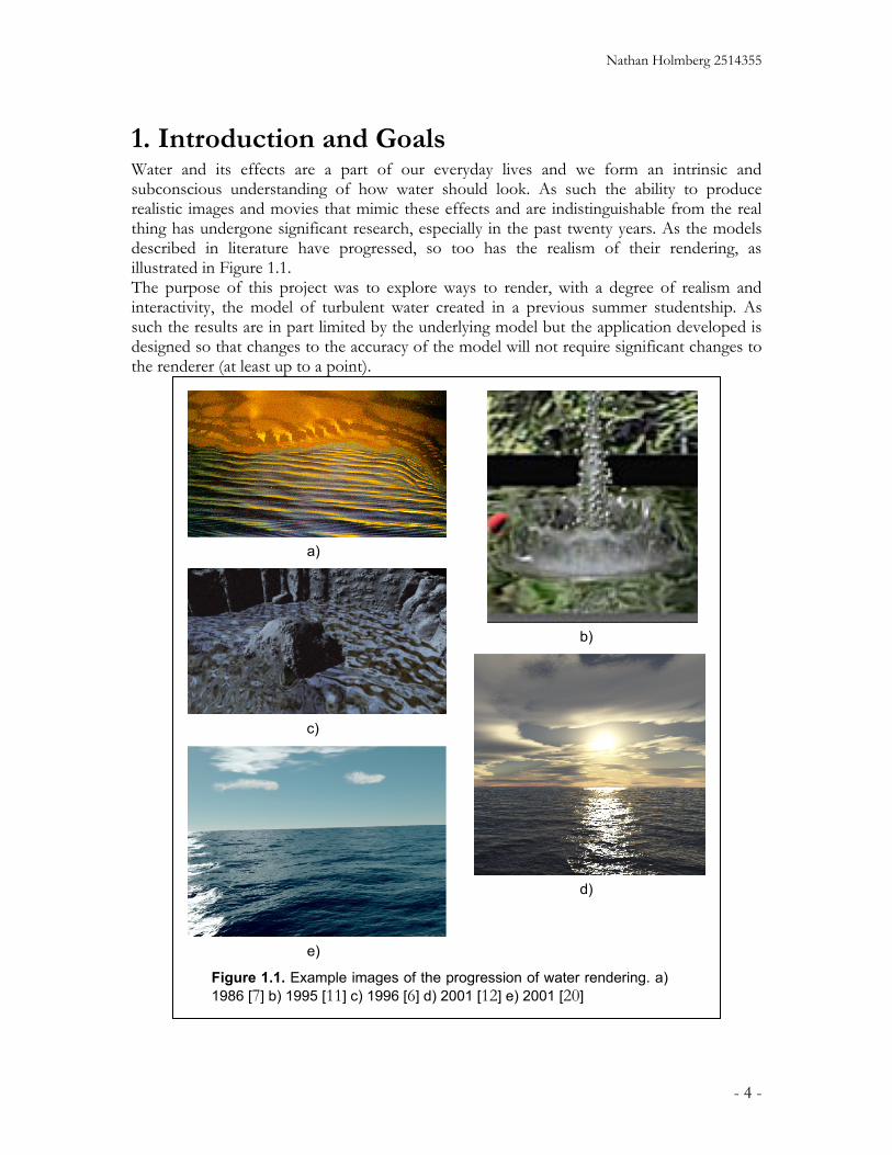
1. Introduction and Goals Water and its effects are a part of our everyday lives and we form an intrinsic and subconscious understanding of how water should look. As such the ability to produce realistic images and movies that mimic these effects and are indistinguishable from the real thing has undergone significant research, especially in the past twenty years. As the models described in literature have progressed, so too has the realism of their rendering, as illustrated in Figure 1.1. The purpose of this project was to explore ways to render, with a degree of realism and interactivity, the model of turbulent water created in a previous summer studentship. As such the results are in part limited by the underlying model but the application developed is designed so that changes to the accuracy of the model will not require significant changes to the renderer (at least up to a point).

a)

b)

c)

d)

e)

Figure 1.1. Example images of the progression of water rendering. a) 1986 [7] b) 1995 [11] c) 1996 [6] d) 2001 [12] e) 2001 [20]


- 5 -

This application was also to be designed as a tool for animators to use to create videos and still frame renderings of water. This means that a greater degree of user interface design and control was sought after and is apparent from the implementation. Another effect of this goal is that a certain level of interactivity is needed for the tool to be useful so while real-time rendering is not possible different methods with different levels of interactivity need to be provided and wherever something is going to take an inordinate amount of time the user has to be made aware of this. In an effort to develop the best possible representation of the model it was also deemed necessary to try to implement as many as possible different methods with a view of comparing the results of each, however time constraints have meant that for some of the intended techniques only a discussion has been provided as implementation was not possible. Finally, this project is a little different as it builds on work that was done previously and uses a model that already exists. Information on this model and what it includes can be found in Appendix A

2. Water Surface The majority of the work done for this project has revolved around finding a realistic representation for the main body of water. This was viewed as the most important feature as not only does it represent the most water by volume but humans are naturally attuned to how water looks and its behaviour under various light. The three methods presented here define a progression from the original mode that constituted a very poor representation through a similarly OpenGL based method of smoothing the surface into the raytracing method that was finally chosen.

2.1. Original Representation Because the original work that produced the model used here did not focus on graphical representations the original representation was embarrassingly simplistic. The column system was represented in OpenGL by a series of Quad Strips between the centres of columns as shown in Figure 2.1. If the next column to be drawn has a height less than a specific threshold then that column is determined to not contain any water and as such the current Quad Strip is terminated and a new one is formed to represent any water on the other side of the gap. Normals for each vertex are produced by taking the cross product of only two of the adjacent edges. This lack of smoothing results in each quadrangle being distinctly visible and the resultant effect is extremely unrealistic. Example images for this method of representation along with a comparison with others are available in Figure 2.8.

Figure 2.1. How the original surface is generated from the columns.


- 6 -

Figure 2.3. Comparison of degrees of NURBS surfaces. a) degree = 1 b) degree = 2 c) degree = 3 d) degree = 4

a) b)

d) c)

2.2. Tessellated B-Splines When looking for a better way to represent the water’s surface the idea of using an implicit surface such as NURBS immediately stood out. Given that the columns could already be represented by a 2D array of points signifying the tops of each column (as was used in the original representation) it seemed logical to use these as the control points for a NURBS surface as in Figure 2.2. Obviously this means that the surface does not go through each control point but is instead pulled towards them, however given that for lower orders this difference is small and so the amount of information that is lost is not significant. In other words the shape approximation was deemed to be appropriate for the task [3]. If the height for a column was below a threshold then that control point was moved to slightly below the base (and therefore out of view).

2.2.1 gluNurbsSurface The initial implementation used the pre existing OpenGL GLUnurbs object and the gluNurbsSurface methods whose proper use is set out in [22]. This uses supplied knot vectors and control points to tessellate the surface automatically and efficiently. One disappointing revelation, however, was that the libraries used in place of OpenGL did not fully support the storing of tessellated NURBS surfaces, at least in no way that was documented. This meant that whenever the view was changed the surface had to be

Figure 2.2. How the NURBS surface is fitted to the columns.


- 7 -

recalculated, a time consuming and computationally expensive task. The method implemented to create the control points and knot vectors is extremely simplistic, using the tops of columns as the control points and the knot vectors having a uniform distribution. By experimenting with the order of the polynomial it was found that a surface of order 3 (which is equivalent to degree 2) was best as while it is not as smooth as others, it more closely resembles the column positions. Figure 2.3 shows a comparison of orders.

2.2.2. New Implementation As an intermediate step between using the OpenGL provided NURBS methods and attempting to ray trace such a surface it seemed appropriate to create a new implementation which used evaluator methods written expressly for this project. As such a class named NURBSObject was created and can be found in the file ‘Utilities.cs’. This has its own blending functions and several evaluators for different purposes based on the equations given in [3], [8] and [9]. Interestingly, this implementation takes a very similar time, and in some cases less, than the gluNURBS method despite being written at a higher level (see Section 6). The main reason for this is that assumptions could be made regarding the inputs. Firstly, it became apparent that the full NURBS equation was not required as each control point was weighted equally. This means that far less computation was necessary for each vertex. Assumptions could also be made if the knot sequence was uniformly distributed, something guaranteed by the implementation. This means that the position within the sequence can be calculated mathematically instead of traversing the entire sequence until the appropriate place is found. Finally by summing those control points whose associated blending value was not zero it meant that many calculations could be discarded. This involves only using the control points within degree/2 of the position of u and v in the knot vectors, possible due to uniformity and the particular spread of control points. Figure 2.4 contains some of the effects of these assumptions. With regards to the implementation two factors are worth mentioning. First, unlike the gluNURBS method it is possible to store the calculated vertices so once the surface is computed there is very little overhead in moving the camera within the scene, but the second is not so advantageous. When OpenGL decides how many samples to use in both directions the distance on the surface is used. This has not been implemented and so the number of samples to take in both the u and v directions is currently hard coded. Of course changing this shouldn’t be too arduous. For full implementation details please refer to ‘Utiltities.cs’ and ‘ColumnSystem.cs’.

Standard equation for NURBS evaluation:

jipj

n

i

m

jpi

jijipj

n

i

m

jpi

wvBuB

wPvBuBvuS

,,0 0

,

,,,0 0

,

)()(

)()(),(

∑∑

∑∑

= =

= ==

Assuming Rationality:

jipj

n

i

m

jpi PvBuBvuS ,,

0 0, )()(),( ∑∑

= =

=

Using only near control points:

jipj

pa

pai

qb

qbjpi PvBuBvuS ,,

2/

2/

2/

2/, )()(),( ∑ ∑

+

−=

+

−=

=

where a & b are the position of u and v in the knot vectors (calculated assuming uniformity)

Figure 2.4. Simplifications of the NURBS equation


- 8 -

Figure 2.5. Graphical Representation of the Newton Root Finding Method

2.3. Ray traced B-Splines The final surface rendering method used was to ray trace the surface. As the title suggests the surface is no longer a true NURBS surface as all control points have a weight of 1 (making it non-rational) and the spacing between knot vectors is assumed to be equal (making it uniform). Because these properties are assumed in the evaluators the implementation can not handle true NURBS surfaces, hence not using the name even though NURBS is a superset containing the type used here. The following two sections seek to explain how the intersection point between the implicit surface and the ray is found.

2.3.1. Newton Solver Early during implementation it was decided that it would be interesting to try to find the intersection between the surface and the ray without tessellating into triangles and testing each for intersection. Further, tessellation would have required implementing BSP Trees sooner in the project and there was not yet any guarantee that there would be time. This also means that the implementation is slower than necessary but without trying both a true comparison is impossible. Following the methods laid out in [9] and the example code provided with said paper and in [14], the chosen method for raytracing the surface was to use a Newton Solver. This particular method involves first decomposing the ray into two planes, the intersection of which is the original ray. The Newton method, a graphical representation of which is in Figure 2.5, is then used to find how close to the given guess the two planes are with the assumption that the distance to the ray will be the sum of the two plane distances. New guesses are then formed using the tangent at the point of the last guess until the distance is within an acceptable error, stored as ROOT_TOLERANCE. In this case the assumption is that the intersection point has been found and will be returned as such. One important case is when the tangent found after a guess is parallel to the ray. In this case there is no intersection between the tangent and the ray planes and the solver fails. This occurs if the Jacobian matrix is singular and if so the guess must be randomly moved a short distance away, the tolerance for this is called the JITTER_TOLERANCE. The mathematics behind this have not been


- 9 -

Figure 2.6. Column Traversal

included here and the reader is referred to [9] for both a more detailed and eloquent explanation of the basis of this method.

The actual implementation, while heavily reliant on [9] and [14], differed due to unique characteristics of the data. Namely because the surface had null control points, a value associated with an empty or missing column, the solver and evaluator had to deal with situations where the guess was within an empty region. This was dealt with by trying to move outside the region and, if this was not possible, assuming there was no hitpoint near that guess (a reasonable assumption). Likewise because the bounding volumes were formulated differently one of the failure conditions was not relevant. In [9] failure was assumed if the distance for the current guess was larger than for the previous. Because this only holds true if there is little variance in curvature within the bounding volume (as there was with their implementation) this could not be used. The performance of this method is not unreasonable on the proviso that the initial guess is close and so it is essential that the implementation get as near as possible, a process described in the next section.

2.3.2. Getting Guesses Before the Newton solver is even employed guesses as close to the proper intersection must be sought. This section describes how this was achieved. First a simple axis aligned bounding box is used to check if the ray comes anywhere near the water surface. In so doing we also determine the first face of the box to be intersected which, because the columns are also axis aligned, provides a starting point and direction for traversing across the scene (the hitpoint on P0x in Figure 2.6). The ray is then intersected with the


- 10 -

plane that describes the edge of the next row of columns (P1x) providing a sub portion of the ray. For each column it passes over between P0x and P1x it is first determined if the ‘y’ value is within the possible bounds of the column (taken as the minimum and maximum of all columns in the area around the target column). If so then the midpoint of the column is submitted as a guess point to the Newton solver which tries up to 5 iterations (defined by MAX_ITER in the code) to find a root. If one is found then it is perceived to be the first hit point on the surface and is returned to the ray tracer, if not then the next column is checked. Once all columns between P0x and P1x are checked then columns between P1x and P2x are checked and so on till either a hit is found or the ray leaves the area defined by the surface. Should the ray have been more orthogonal to the ‘z’ axis than the ‘x’, then it would have been P0z, P1z and P2z that were used. One advantage of this method is that because it both ensures that the first hit point will be returned and that each guess is relatively close to where the intersection may be, due to the small amount of movement in the ‘u’ and ‘v’ values that can occur between columns which represent the width of the greatest possible error. On the other hand its efficiency is very dependant on the number of columns in the system and how many columns each ray passes over before hitting the surface.

2.4 Worthwhile Additions One interesting benefit of using B-Spline surfaces that has not been implemented but is worthy of mention is the effect that could be achieved by offsetting each control point slightly depending on the position of each column. This would allow for the simulation of adhesion along boundaries and possibly viscous shear, two things currently missing from the underlying model. Figure 2.7 provides an indication of how this might work. Likewise using flow and pressure information between columns could be used to identify areas of high turbulence and a texture be generated that simulates the high air content of the water at such places, i.e. foam.

a) b)

Figure 2.7. The effect of slightly displacing control points. a) Unaffected b) Edge points moved against the flow


- 11 -

Figure 2.8. A Comparison of the three draw methods used. a) Original b) gluNurbs c) Ray traced. Example videos are provided for a better comparison

a) b) c)


- 12 -

3. Particles The second major feature of the model that needed to be represented was the particle system. This system was used to account for any activity that required water to break away from the main body of water and as such included a variety of effects. As these range from small whitecaps on the tops of waves, through spray from water impacting on rocks, to laminar like flow over waterfalls it was unlikely that a simple method would be sufficient. With this in mind a variety of techniques were investigated and while only a few were able to be implemented the others are included with a discussion on their relative merits.

3.1. Original Representation The original representation for water particles was to use the glutSphere object provided by OpenGL. Each particle was represented by one sphere the radius (and therefore size) of which was determined by the volume of water that the particle was supposed to represent. Some effort was made to differentiate between types of spray by using the velocity and ‘timeAlive’ attributes of each particle to alter the colour and opacity of the representing sphere. However the effect this generated was disappointing and was eventually disbanded when work began to focus on raytracing. This method was used for the first three attempts and little work was done to progress the way particles were represented until ray tracing began.

Figure 3.1. Original Particle Representation


- 13 -

3.2. Ray Traced Particles Ray tracing particles presents particular problems. Namely due to the possible numbers (up to 100,000 in some scenes) it is far too time consuming to test for ray intersection with each one. As such an acceleration technique known as BSP Trees was used and a discussion of this appears in the first section. There is also the problem of how different splashes appear to have different properties and so the ray tracer would have to implement several different methods of representation, while not all of these were completed an overview of the technologies that could be employed is included along with a description of where they might be useful.

3.2.1. BSP Tree Basics The only acceleration technique that was implemented during the course of the project was a simple Binary Space Partitioning Tree. This technique splits the system into two at each step and creates a tree of these partitions. This tree is then ray traced with the ray being passed down the branches of the tree in such a way that the minimum number of intersection calculations need be performed. Normally when implementing BSP Trees care has to be taken that a partitioning plane does not intersect an object. However due to the fact that only particles are contained within the tree this has been disregarded as the chance of plane / particle intersection is very slim. Of course this also makes the implementation easier. After implementing BSP Trees a decrease in rendering time of between 4 and 5 times was realised. While this is good it is not as large as might be expected, possibly due to the relatively ‘flat’ nature of the particle’s distribution and the simplistic division algorithm that

will mean that most division will only be with planes perpendicular to the x and z axes. This algorithm is demonstrated in Figure 3.2 with the following explaination. First an axis aligned bounding box is fitted to the particles. This is then subdivided into two along it longest side creating two smaller boxes and a division of the particles accordingly, thee two boxes are also split, again along the longest axis, and the process continues until the

Figure 3.2. BSP Tree creation. NB. The unevenness of the tree shown is actually quite likely due to the concentration of particles in certain areas and the simplicity of the algorithm used for partitioning.


- 14 -

maximum tree depth is reached or there is less than a threshold number of objects within a box. The implementation was derived primarily from the start point of an assignment for COMPSCI715 and as such does not constitute the most efficient implementation. For the program structure and details of this implementation please refer to Appendix B and the file ‘Raytracer.cs’.

3.2.2. Spheres The first method used to represent particles is very similar to the original representation discussed previously. Simply put this involves ray tracing a sphere at the position of each particle. Because ray sphere intersections are perhaps the fastest and easiest this translates to a ‘reasonably’ fast method. Of course without the BSP Tree this would still be daunting Result looks similar to the original representation, as one might expect, but there are still possible uses for this method. Namely very dispersed sprays of large droplets, such as those created after a smooth splash breaks up, could be represented by this method. To achieve this, a combination of the ‘time alive’ and a check as to the how far the nearest neighbour is could be used to transition between another method and this.

Figure 3.3. Using spheres to represent particles


- 15 -

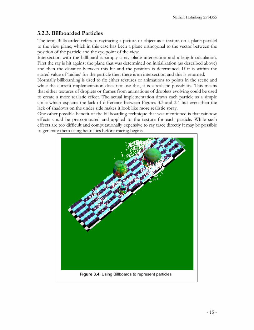
3.2.3. Billboarded Particles The term Billboarded refers to raytracing a picture or object as a texture on a plane parallel to the view plane, which in this case has been a plane orthogonal to the vector between the position of the particle and the eye point of the view. Intersection with the billboard is simply a ray plane intersection and a length calculation. First the ray is hit against the plane that was determined on initialization (as described above) and then the distance between this hit and the position is determined. If it is within the stored value of ‘radius’ for the particle then there is an intersection and this is returned. Normally billboarding is used to fix either textures or animations to points in the scene and while the current implementation does not use this, it is a realistic possibility. This means that either textures of droplets or frames from animations of droplets evolving could be used to create a more realistic effect. The actual implementation draws each particle as a simple circle which explains the lack of difference between Figures 3.3 and 3.4 but even then the lack of shadows on the under side makes it look like more realistic spray. One other possible benefit of the billboarding technique that was mentioned is that rainbow effects could be pre-computed and applied to the texture for each particle. While such effects are too difficult and computationally expensive to ray trace directly it may be possible to generate them using heuristics before tracing begins.

Figure 3.4. Using Billboards to represent particles


- 16 -

Figure 3.6. Example of implicit water surface generated from particles. Image from [13].

Figure 3.5. Example of Illuminated Streamlines as used in CFD [23].

3.2.4. Illuminated Streamlines Another method that was reviewed as a possible alternative for spray was illuminated streamlines. Typically it is impossible to render a one dimensional figure such as a line in a ray tracer as there is no one normal to use in lighting calculations. This can be overcome by using the normal which is in the same plane as both the line and the direction from the hitpoint to the light source, enabling proper effects [23]. While most of the usual uses and properties set out in the literature are not applicable, this technique was looked at because of its ability to simulate very fast moving splashes and spray, as is the case in aerated waterfalls etc, and what might be called a motion blurring effect. Figure 3.5 shows how some of these effects may look and a partial implementation can be found in ‘RayTracer.cs’.

3.2.5. Texture Splats & Volume Rendering The final method thought of for raytracing is the use of texture splats or some type of volume rendering to create the impression of fine mist, as is often found in areas where spray rejoins the main body of water at high velocity such as at the base of waterfalls. In these areas spray takes on some of the characteristics of fog and so the techniques that were investigated largely stem from attempts in this area. Raytracing volumes such as this is related very closely with simulating the scattering of light underwater and including one might form the basis for the other.

3.3 Implicit Surfaces One of the most promising representations that were not implemented was the possibility of using implicit surfaces to create a solid object, the shape of which is determined by the particles. Such a method would be perfect for laminar flows that exist outside the column system, the most important of which would be over waterfalls. The current methods employed all disregard effects where particles are in close proximity so make such flows look either more turbulent than they are or highly unrealistic. While this may look nice, however, it would take considerable computation to use the marching cubes algorithm (for example). More recently


- 17 -

Figure 4.1. Reflection vectors: n = surface normal d = ray direction r = new ray direction a = parallel to n, scaled by d θ = angle of incidence

Figure 4.2. Refraction vectors: n = surface normal d = ray direction b = tangent to the surface θ = angle of incidence θ’ = angle of refraction

(November 2003) work has been published which have implemented a surface over particles specifically. [13] presents a method of water simulation using only particles and represents the surface using ‘level set methods’ although this would involve possibly rewriting parts of the underlying model it would achieve the required effect, the results of this are demonstrated in Figure 3.6.

4. Supplementary Effects This section describes some of the effects that had to be included with the ray tracer and while important for realism are not directly related to either the water surface or particles.

4.1. Reflection Reflections are probably the simplest and most important effects that could be included. This involves creating a second ray for each hit on a reflective surface which is used to find the colour to be reflected. This continues for as many iterations as is specified by the programmer (in this case 2 because the scene is unlikely to have many multiple reflections of importance) or until a ray hits the background or non-reflective surface. Following the premise that the angle of incidence is equal to the angle of reflection we can deduce that:

adr 2+= and using the formula for orthogonal projection we can find a such that [17]:

nnnddr 2||||

2 •−=

The basic diagram illustrating this relationship can be found in Figure 4.1. As will be discussed in the next section, the resultant reflected colour must be scaled by a factor depending on the absorption properties of water and the size of the angle of incidence.

4.2. Refraction The second effect discussed here is that of refraction. This refers to the bending of light as it passes from one medium to another that has a different refractive index. Water is one such material and has a commonly accepted refractive index of 1.33 compared to the 1.0 of air. The mathematics for calculating the direction of


- 18 -

this ray is a little more complicated but still simplistic and one of the most commonly taught. The relationship between vectors can be found in Figure 4.2 and the equation to find t (the transmitted ray) is as follows:

22

221

2

1 ))(1(1))((n

ndnnn

ndndnt •−−−

•−=

where n1 and n2 represent the refractive indices of the two materials (in this case air and water). In terms of the model, refraction is important due to the distortion effect it has on the ground. This allows the movement of waves to be seen even if there are not enough highlights to show them explicitly. This can be seen in Figure 4.3.

4.2.1 Schlick’s Approximation Water is also a dielectric (not to be confused with conductive properties) which means that the intensity of the refracted vs. the reflected ray varies according to the angle of incidence. The typical operation of such is that as the angle of incidence (θ) approaches zero the transmitted ray approaches one and the specular reflectance approaches zero. The Fresnel equations are commonly used to describe this relationship but are difficult to compute. As such, the standard equations used in ray tracing are those proposed by Schlick in [16] and are reffered to as Schlick’s approximation. This approximation does not provide exact answers and are only valid for unpolarized light but given that ignoring polarization probably creates even larger errors, this error is seen to be inconsequential, a view shared by [17]. The equations that were used to govern this relationship for reflectance (R(θ)) and transmittance (T(θ))are as follows:

500 )cos1)(1()( θθ −−+= RRR

and from the conservation of energy )(1)( θθ RT −=

Figure 4.3. Image showing the effect of refraction on the appearance of the ground plane.


- 19 -

(a) (b)

Figure 4.4. a) Flat coloured sky. b) Using the texture map ‘CloudTexture.bmp’ which includes clouds. Both images use a non-transparent water surface

Where R0 is the base reflectance set by the user and cos θ can be determined by –d•n making the formula computationally inexpensive. It should be noted that this relationship is only used for transparent surfaces where refraction is expected to occur in the model and its effect is discounted for the ground panels and spheres etc.

4.3. Skybox In simple ray tracers, if a ray does not hit any of the objects in the scene it is given the standard background colour. This however is unrealistic especially when dealing with reflections off the surface of the water. As such, the inclusion of a skybox for the ray traced surface turned out to be very important in creating an added sense of realism. Most non-ray traced programs use a texture mapped bounding cube that is used when there is no object between the eye and infinity and while this is good for programs such as games it would greatly increase the computation necessary for each ray that hits the ‘background’. Because of this an easier method which uses only the direction of each ray to determine a hitpoint on a sphere was used, the idea for which was gleaned from [5]. First the world is divided into two by the ‘y’ direction of the ray creating a horizon, namely if it is positive then the sky texture is used and if it is negative the ray is pointing at the ground. The problem then becomes a simple matter of texture mapping a sphere, namely creating u and v coordinates and extracting the texture value for that coordinate from the texture map. Namely, where x, y, and z represent the normalized direction (and so the radius is one) [17]:

π2),(2arctan xyu = and

ππ )/arccos( rzv −=

Of course these are the equations for the standard case and so only half of each texture map will be used but given the distortion of applying a square texture to a sphere this was not seen as a major problem to be solved given time constraints. Also due to these constraints no interpolation of the texture maps has been implemented, meaning that looking directly at the sky is not a particularly pretty sight but this is offset by


- 20 -

Figure 4.5. How the generation of light caustics may work

the more realistic reflections that are generated off the water, as demonstrated in Figure 4.4. The implementation for this can be found in ‘RayTracer.cs’ starting on line 323. As is common with skyboxes no illumination effects can be seen on the background and may have to be manually applied to the textures if this is so desired.

4.4. Accepted Property Values This section documents the values that were used for various properties of water. In most cases these values were chosen because ‘they looked good’ and are not representative of the true values. That said some are based on experimental data and are referenced accordingly. Table 4.1 contains these values.

4.5. Worthwhile Additions One of the most notably missing effects that this model would benefit from is light caustics. This refers to the areas of higher intensity light which are collated due to the refraction of light through the water gathering in specific regions. They are a sure sign of wave motion on the surface and one of the effects that the human eye expects to see. The reason that this wasn’t included in this project is that including light caustics would require another pass of the ray tracer to generate a second texture for objects in the environment. This would require significant changes to the program as it stands, and while a partial implementation was possible completion was precluded by the time available. The following details how such effects may have been achieved, as was usual for this project however, it details a conjectured theory only that has not been proven yet. By using rays defined by the position of the light source and sample points on the water surface it should be possible to use the refracted instance to find the point on the ‘ground’ that would be illuminated by the light, as in Figure 4.5. If enough of these

Table 4.1. Values used for various water properties. Where three values are given they correspond to the red, green and blue channels respectively

Property Name Value Used Diffuse reflectance {0.1f,0.1f, 0.3f} Specular reflectance {0.7f,0.7f,0.8f} Phong exponent 1000 Specular transmittance (absorption) {0.34f,0.05f,0.009f}


- 21 -

sample rays are used then a map of hits can be built up and using the density of these hits a texture created that illustrates where light is concentrated and diffuse. This method would also work for multiple light sources with the algorithm being repeated for each. A second missing effect is how the depth of water changes its colour and the scattering that occurs when photons encounter sediment in the water. Research already exists in this area, the clearest explanation found in [12], and including these effects would be a simple matter of extending the existing program. Of course these are only two of the possible additions. Anti-aliasing, multi-sampling, smoothing etc would all make the renderer better but fall outside the scope of this project.

5. Implementation Overview This section provides an overview of the features, structure and I/O of the program written as partial requirements for this project. The C# language was used as it is easy and fast to implement prototypes in while retaining much of the speed advantages of C++ (if these do in fact exist). Given that the model was also written in this language it seemed a natural progression to write the renderer in it also. While the OpenGL libraries aren’t directly available, a third party, open source implementation called CsGL exists and was used extensively[4]. This provides a wrapper of the actual libraries that can be used with any .NET language (although was written specifically for C#). It is not, however, a perfect translation and there exist idiosyncrasies that had to be dealt with but was more than adequate for what was needed here.

5.1. Input The input for the program written for this project is in the form of files representing the scene and the positions of the water. The first step of this project was in fact to alter the program written to model water to output this information into proper files (previously the only output was in the form of bitmap images). While the model data used was produced in a previous project this is not the only possible source of data. To separate the two programs a format was created to serialize and deserialize information about the scene. While this was originally intended to allow pre-computed scenes to be used in the rendering process it also means that any file following the format set out below could in theory be used. For any sequence of scenes there are two types of files needed. The first is a static file containing information about the scene and the second contains information about the position and state of water at each time step. The static file, whose default name is ‘model.state’ typically contains the bare panels and spheres as used by the original modeller but was intended to be extended or replaced between the modelling and rendering process. This means that more complicated /realistic scenes could be used in conjuncture with the data created by the modeller. For each time step there is a separate file, named ‘time###.state’, where ### refers to numbers which are incremented with each frame, retaining the ordering. These files first contain information on the position of the first column and what the heights and widths of every column will be. It is from this information that the positions of all the other columns will be determined. For each column the heights of the base and top are stored along with information on the pressure and rate of flow (in 2D). This information was kept as it may


- 22 -

help with rendering while all information regarding pipes and the cells within columns are discarded. Particle information is also stored in this file with the position, velocity, mass and the length of time alive being stored for each. For the actual implementation information please refer to the source file ‘Serialization.cs’.

5.2. Operations The ModelView program, the main method of which resides in ‘ModelView.cs’, which forms the basis of the project is a GUI based interface designed to allow as much control over the animation process as possible. The order of operations is quite simple. Using the interface provided by the button ‘Select Files’, the static file containing information about the scene and the instance files containing the water at each time step are selected. This creates an array of filenames, but does not load anything, and the trackbar is initialized to have as many points as are needed. The ‘Load Files’ button is then used to either load the single file representing the select time step or to load and store all instances in an array. This distinction was made to allow for times when the complexity of a scene or the available memory precludes loading all time steps at once. This will also initialize the OpenGL panel with the selected time step’s information and the default view. This can then be manipulated using the trackball and camera controls provided by ‘Trackball.cs’. These are based almost exclusively on those provided for various COMPSCI372 assignments and operate in a way that should be familiar to those who have used these and similar programs before. A ‘Controls Enabled’ option is also provided to ensure erroneous mouse movements don’t change the camera position between frames, if so desired. Changing the selected ‘Render Type’ will automatically redraw the scene and wile there is no indication of progress for the original and tessellated NURBS based methods, when ray tracing another window will open which includes a rudimentary indication of progression (based on the number of pixels calculated). Example shots of all the user interface screens are provided in Appendix C.

5.3. Setting up the Ray Tracer This section was included as one of the features of the program is that any view chosen using the OpenGL based rendering methods can be replicated exactly for the ray tracer. This overcomes the fact that interactivity is prohibited by the length of time it takes to ray trace each frame by allowing navigation and camera position to occur before ray tracing. It is also important as the trackball and camera controls don’t actually work for the ray traced view. The ray trace view is composed of an eyepoint, direction, up vector, a distance and size of the ‘viewing plane’ and the number of pixels to sample in each direction. The particular implementation I chose was to choose an arbitrary size of the ‘viewing plane’ (s) and derive the distance (d) from the required zoom (fov). This is achieved by the simple formula below:

)5.0tan(2 fovsd =

For the eyepoint, direction, and up vector the information regarding these three factors used in the gluLookat() command are multiplied with the current transformation matrix (as created by the trackball object) to create the proper viewpoint. While it is relatively simple the effect it has on interactivity is marked.


- 23 -

5.4. Output Output is in the form of either bitmap or JPEG encoded images although due to quality concerns only the bitmap methods are currently used. There are two events that generate these images. The first is whenever a ray traced image is completed. Due to a peculiarity of CsGL the image isn’t shown as it is generated and because render times were sometimes ludicrously long it was deemed better if output was directly to an image file on the hard disk. Failing this the ‘Render’ button on the interface either captures the current view or, if the ‘Batch Render’ option is selected it loads each of the selected time steps and renders each to a different file. This automates the process of creating frames for animation so there is no need for a human operator to choose the next frame, especially important when ray tracing can mean that each takes several minutes. In the case of a single frame capture the filename follows the format of “time <date> <time> method <method number>.bmp” where <date> and <time> represent the current date and time and <method number> represents the ‘Render Type’ selected. For batch rendered files the format is the same but with “Frame <frame number>” prefixed which provides an ordering mechanism for the output files. For the methods used to convert pixel information into these file formats please refer to ‘Utilities.cs’. These bitmaps are then used with the open source program ‘MakeAVI’ [15] which converts them into avi files using whatever codecs are available.

5.5. Worthwhile Additions While one of the original goals was to create a tool that could be used by animators wishing to simulate the movement and effects of water, the majority of work has focused on implementing rendering methods and the theory behind different techniques. As a result there were several things which were not implemented but would help towards this aim. The first would be to include in the interface the capability to explicitly set a view. This would enable a more accurate comparison of angles and an ability to use the same view on several computers (if rendering separate frames of the same sequence on different computers). Currently this has been hardcoded when required. The second worthwhile addition, namely the ability to set water properties and environmental effects (such as the sky texture and light positions) is currently much the same. If this information is either stored in a configuration file or accessible through the user interface, a greater degree of flexibility and control would be afforded. While these two additions are largely superficial the final and most important would be the ability to set camera paths through scenes that would be followed as frames are rendered. This would greatly enhance the usability of the program as a rendering tool for animators and should produce interesting effects, especially with moving highlights etc.


- 24 -

6. Conclusion & Results The results presented here represent only some of the work that could be done towards this subject and needless to say it is limitations on time and resources that have precluded a full study, but the initial results look encouraging. In the end several rendering methods used at different stages of the production process seems to be the best answer with, for example, the original representation being adequate for finding the best possible view while the OpenGL based tessellation methods give an idea as to what the shape of the surface will look like. For the final rendering ray tracing seems the most obvious choice but even within this different techniques could be used for different effects, especially when treating spray. Billboarded particles, illuminated streamlines, texture splats and implicit surfaces would all be useful for simulating various types of spray and laminar flow such as that over waterfalls. The application developed also provides the required interactivity and a tool for animators with extensions possible as discussed Section 5. However, while it may be that all are useful one of the goals called for a comparison of the techniques and so Table 6.1 contains some time-based information on how they compare. It is important to note that the implementation as is stands is really just a proof of concept and is not at all efficiently coded. In particular the code for the BSP trees are very raw, a possible explanation for the appalling times shown in the table.

The time for ‘first’ drawing includes initialization etc while ‘next’ doesn’t Small Scene: 80x20 columns, 2800 particles Large Scene: Test System: Athlon XP 2100 w/ 512MB RAM

Table 6.1. Rendering Times of different methods

Description Time taken (First / Next)

Original Representation – small scene 60ms / 15ms gluNURBS – small scene 1600ms / 1400ms New Implementation – small scene 4000ms / 1200ms Raytracing – small scene 500x500 380000ms Raytracing – small scene (surface only) 86000ms Raytracing – small scene (spheres only) 104000ms Raytracing – small scene (Billboarded only) 230000ms Original Representation – large scene 700ms / 500ms gluNURBS – large scene 20000ms /19000msNew Implementation – large scene 9000ms / 1400ms Raytracing – large scene 500x500 5400000ms Raytracing – large scene (surface only) 4780000ms Raytracing – large scene (spheres only) 400000ms Raytracing – large scene (Billboarded only) 1400000ms


- 25 -

Appendix A – Base Model This section describes the model that was used to create the data for rendering during this project. It is important to note that the following does not constitute work done during the course of the project and should not be seen as such.

Volume Model Continuing the work of O’Brien & Hodges and Mould & Yang [10] [11] the volume model, representing the main body of water in our model, is a column based system. Using columns holds the advantages of easy surface creation as the top of all columns are known and less flow calculations needed so the system is less computationally intensive.

The structure of the volume model is much the same as that used in the previous work mentioned above. That is the environment is divided into equal sized squares which form the base of columns as in figure 2. All columns start with a user defined height which then varies over time dependant on the calculated flows. Source / sink columns are the only ones to retain their heights allowing for in and out flows to the system. Pipes are then created between each of the eight adjacent columns and each cell that could overlap during the course of the simulation. Pipes are also created between the cells of one column and the air above the adjacent columns. At this point the system is

ready to begin simulation. The underlying basis for the flow equations that are used in this simulation is the science of hydrostatics, or that describing the pressure of fluids at rest. The equations related with this approach are simple, both to understand and to compute, and as a result are easy to implement. For any column in the grid the hydrostatic pressure can be calculated from the equation below based on the work of Bernoulli.

)(21

02 EpvghQ +++= ρρ

Where Q is the total pressure, h the height of the column, g acceleration due to gravity, ρ the density of the fluid, v the velocity of flow. p0 the air pressure and E the pressure arising from external forces which together form the pressure energy term. In this case the height of the column is the height above some arbitrary point in the world so long as the same point is used for all columns.

a) Environment before columns are generated.

b) Top down view with environment split into grid for columns.

c) Columns after generation with initial heights.

Figure A. Column Generation from environment. Arrows indicate position of some pipes.


- 26 -

Using the pressure differences between cells it is possible to calculate the acceleration and from that the flow that should occur between cells. The final equation for the flow velocity (η) through a pipe is:

)(0 lQQ

tf tailhead

ρηη −

∆+=

Where l is the pipe length, f is a friction coefficient (as suggested in [10]), and η0 is the flow in the previous time step. An interesting point to note is the lack of any viscosity parameter in this equation. This is because one of Bernoulli’s assumptions was that the distances between points of measurement were so small that viscous losses were negligible, instead the friction coefficient used allows energy to slowly escape from the system. While not physically justified it serves as an ad-hoc method of including viscosity and in all examples was set at 0.995. Using the flow calculated for the pipe the volume of water that should be moved through it is calculated by:

ctV η∆= Where c is the cross-sectional area of the pipe, or the amount of overlap between the cells. Because mass is to be conserved the volume removed from one column is the same as that added to the other. Care must also be taken not to allow a volume of less than zero to occur. This system is very fast considering the mass of water that is being represented but there are several problems. Columns pose a problem as a representation because turbulence is a three dimensional feature; this is considered one of the classical characteristics of turbulence [1]. While using the ‘cells’ given by Mould & Yang relaxes the assumption of vertical isotropy this goes a long way to explaining some of the model’s inability to simulate certain situations. A second problem arises from the fact that turbulence is a feature of flow and not of the fluid ‘at rest’. This means that while hydrostatics may be easy to use the equations generated for flow are incomplete and ignore many of the visible characteristics of water such as shear stresses. This is perhaps the largest flaw in the model and something that lends itself to further research.

Spray Model The spray model is used to model water as it breaks free of the main volume of water. There is no easy physical solution to when spray should be created and as such assumptions must be made instead. Earlier work with column systems were concerned mainly with generating splashes from hitting objects and as such used vertical velocity thresholds for generating spray. Because the idea here is to model waterfalls the assumptions used here are those regarding the heights of wave crests before they become unstable (when the wave height is 0.78 of the water depth) [21]. This obviously allows waterfalls to form easily but also works for rapids as large flow velocities form ‘spikes’ of water that while erroneous are then turned into spray due to their large heights. The spray system begins its evolution when particles are generated. First the number of particles (or volume) needs to be determined. Using the formula to calculate flow through a weir it is possible to determine the required flow rate and therefore volume. This is through the equation [2]:

gBHflowrate 232 2

3

=


- 27 -

Where B is the base length, H the height and g the acceleration due to gravity. The volume to pass through in this time step can then be found by flow rate * time step. This determines the number of particles to be created as all those generated, except the last, is of a user defined volume. The last of course needs to be the remainder of volume to be moved as mass must be conserved and not created. Depending on the scale and resolution of the model currently being used this can be set to achieve the best looking results. The position of the particles is also easily determined and is set at a random position in the face that the particle is being generated from. The final initial variable that is needed for each particle is velocity and this can also be generated from the flow rate equation above. In this case the velocity of flow through a column’s face is found to be flow rate / face area. Flows within the column structure may mean the velocity should not be perpendicular to the front of the face; to account for this the average flow from surrounding columns is used to give direction to the scalar velocity calculated above. In many cases the velocity imparted to the particle should not only be horizontal but also include an initial y velocity. To do this the difference in total height between the column for which particles are being generated and the column behind is used in the classic formula

asuv 222 += Where v is the current velocity, u is the initial velocity, a the acceleration, in this case gravity, and s the distance covered. While this may not be a perfect physical solution it does manage to provide a more believable representation. One of the methods that were initially considered to help create the illusion of water pooling and incompressibility was the use of cohesion. This involves creating small forces between water particles which attract and repel neighbours in the effort of keeping an optimal distance apart and is an effort to model intermolecular bonds. After both observing the inefficiency and inaccuracy of using cohesion within the particle system and after reading enough to convince that such was unneeded due to water’s low viscosity so long as the movement was turbulent, such as is the case with spray, [18][19] this was excluded when the particle and column systems were combined. The visual effects of such cohesion might be achieved by appropriate rendering of the particle system but due to time constraints we were not able to explore this topic in more detail. This means that the only active force during a time step is gravity. Collision detection with the boundary is the same as for the original particle system described in the implementation section and so collisions with columns is the only thing explained here. After calculating which column the particle is above (or within), the particle’s y coordinate value is tested to see if it should be absorbed into the column. Simply increasing the column’s volume and destroying the particle was found not to be accurate enough however as this would force the column’s height up, often absorbing more particles in the process. This would not have been a problem for the small scale splash effects that the underlying model was designed for but causes considerable problems when the particles are modelling waterfalls where there are many particles hitting at any one time. After trying to spread the volume of a colliding particle over several columns it was found that by instead modelling the force of impact and subsequent pressure increase in the column not only was the problem reduced but more realistic effects were generated. The equations used were the same as for external objects colliding with the water presented in Mould and Yang. The force on the object is given as two terms.

gVvF ρµ −−=


- 28 -

Where v is the velocity of the object, µ is the viscosity, V the volume of water displaced, ρ the density of the fluid and g the acceleration due to gravity. The first term describes the force of the fluid on the particle and the second is the force due to buoyancy. Because the force on the fluid must be equal but oppositely orientated to that on the water droplet this formula can then be used to determine the force on the column. Using the formulas:

AmP /= and aFm =

We can then calculate the resultant pressure of this force on the column, stopping it from rising unrealistically.


- 29 -

Appendix B – Program Interface and Structure User Interface This section contains example screens of the user interface with descriptions of the various features.

Main Window This window is initially presented to the user and provides the majority of available options

1) OpenGL window – This window shows the current output, clicking and dragging anywhere within the program activates the trackball and allows the user to change the view. Likewise the camera control keys will change the view here

2) Rendering Method – Changing the method by clicking on a new radio button will redraw the OpenGL window with the desired method

3) Controls Enabled – If selected the trackball and camera will be active, otherwise user interaction is halted

Figure B.1. Main Window User Interface


- 30 -

4) Batch Render – If selected the ‘Render; button will cycle through all loaded time steps, outputting the results to sequential filenames.

5) Load Files – Once Files have been selected this button will either load a single time step into memory or all those selected (depending on the value of (8))

6) Select Files – Opens the Select Files dialog to allow the user to select those files representing the background scene and water at each time step.

7) FPS – Frames per second. Not very important but changes how the ‘Current Time’ value in (10) is incremented

8) Load Options – Determines if all or only one time step will be in memory at a time. Helpful when dealing with very large files.

9) Render – Captures the output window to a file or, if ‘Batch Render’ is selected, renders all frames using the current view and method.

10) Controls – Allows the user to navigate between loaded time steps using the trackbar.

Select Files This window is presented to the user to allow them to select the relevant static and instance files as described in Section 5.1.

1) Select Files 1 – This area allows the user to navigate to the directory in which files the files relating to each time step are stored.

2) Select Files 2 – This are allows the user to select filenames from the currently selected directory to use as either the static or instance files.

3) Select/Remove Static – Uses the file currently selected in (2) as the static file or removes that displayed in (6)

4) Select/Remove Instance – Similar to (3) but allows for multiple selections and governs the contents of (7)

5) Clear All/OK – Either resets the form or accepts the currently selected files and informs the main program that a new selection of files is ready to be loaded

Figure B.2. Select Files User Interface


- 31 -

6) Static State File – Displays the current file that contains information relating to the position of background objects such as rocks and ground panels.

7) Instance State Files – Displays the selected files that contain information on the position of the water at each time step.

Progress Window Due to the time that raytracing can take, a simple progress window was included. This runs in a separate thread and allows the user to cancel the raytracing at any time. An image is still saved in these cases to allow the user to see what the image may have looked like The progress itself is actually a simplistic calculation based on the number of pixels already calculated and the number remaining, regardless of how complex the scene is behind each of these pixels. As a result it is not uncommon for the progress bar to proceed in fits and starts as simple areas (where only the background is drawn) are completed.

1) Resolution – Displays the resolution being used for the current image in Width x

Height format 2) Start/End Times – Displays the system time of when the ray tracing started and, on

completion, when it stopped 3) Percentage Complete – Provides both a numerical and visual representation of how

much of the image has been completed 4) OK/Cancel – Allows the user to stop the ray tracer at any time. Needless to say the

OK button is only available when the ray tracer has completed

Camera Control Keys The following lists the keyboard controls for camera operation: Z/X – Zoom in / out of scene Q/E – Increase / Decrease the elevation of the camera R/F – Raise / Lower the position of the camera (in the y direction) A/D – Rotate the camera on its y axis W/S – Move the camera forward / backward along its current direction

Class Diagram The class diagram on the following page was created after implementation, which explains some of the strange design. The diagram also does not include all attributes or methods as these can be found already in the implementation if required.

Figure B.3. Progress Indication User Interface


- 32 -

Figure B.4. Class Diagram


- 33 -

Appendix C – References [1] Abbot M & Basco D. (1989). Computational Fluid Dynamics – An Introduction for Engineers. Longman Scientific & Technical. [2] Badger W & Banchero J. (1955). Introduction to Chemical Engineering. McGraw-Hill. [3] Cohen, E. et al (2001). Geometric Modeling with Splines: An Introduction, A K Peters, Massachusetts, 2001 [4] Dupont, L. et al (2003). CsGL – C# graphics Library. http://csgl.sourceforge.net/ Viewed last on 9/11/03 [5] Feasel, J. (2003). World’s Slowest Ray Tracer. http://www.cs.unc.edu/~feasel/classes/236/raytrace.html Viewed last on 9/11/03 [6] Foster, N. & Metaxas, D. (1996). Realistic Animation of Liquids. Graphical Models and Imaging Processing: GMIP V. 58 n 5:471-483 [7] Fournier, A. & Reeves, W (1986). A Simple Model of Ocean Waves. SIGGRAPH ‘86 [8] Grahn, H. et al (1999). NURBS in VRML. In Proceedings of the Web3DVRML, 1999. [9] Martin, W et al (2000). Practical Ray Tracing of Trimmed NURBS Surfaces. Journal of Graphics Tools V. 5 n 1:27-52 [10] Mould D & Yang Y. (1997). Modeling water for computer graphics. Computer & Graphics V. 21 n 6:801-814 1997 [11] O’Brien J & Hodgins J. (1995). Dynamic Simulation of splashing fluids. Computer Animation ’95:198-205 [12] Premože, S. & Ashikhmin (2001). Rendering Natural Waters. Computer Graphics Forum V. 20 n 4:189-200 [13] Premože, S. et al. (2003). Particle Based Simulation of Fluids. Europgraphics 2003 V. 22 n 3:401-410 [14] Press, W et al. (2003). Numerical Recipes in C: The art of Scientific Computing (2nd Edition). Cambridge University Press, Cambridge [15] Ridley, J (2003). SourceForge.net: Project Info – MakeAVI. http://makeavi.sourceforge.net/projects/makeavi/ Viewed last on 9/11/03 [16] Schlick, C (1994). An Inexpensive BRDF model for Physically based Rendering. Eurographics ’94 V. 13 n 3:233-246


- 34 -

[17] Shirley, P. & Morley, R.K. (2003). Realistic Ray Tracing (2nd Edition). A K Peters, Massachusetts, 2003 [18] Sims K. (1990). Particle Animation and rendering using data parallel computation. SIGGRAPH ‘90 [19] Stein C & Max N. (1998). A Particle-Based Model for Water Simulation. Prepared for SIGGRAPH ‘98 [20] Tessendorf, J (2001). Simulating Ocean Water. SIGGRAPH 2001 Course Notes [21] Thorton E & Guza R. (1982). Energy Saturation and Phase Speeds Measured on a Natural Beach. Journal of Geophysical Research V. 87 c 12:9499-9508 1982 [22] Woo M., Neider J., Davis T. & Shreiner, D. (1999). OpenGL Programming Guide (3rd Edition). Addison & Wesley, New Jersey, 1999. [23] Zöckler, M. et al (1996). Interactive Visualization of 3D-Vector Fields using Illuminated Stream Lines. IEEE Visualization ’96 Conference p. 107

Rendering of Turbulent Water over Natural Terrainburkhard/Reports/2003_S2_Nathan... · Rendering of...

Documents

Transcript of Rendering of Turbulent Water over Natural Terrainburkhard/Reports/2003_S2_Nathan... · Rendering of...