Remote Sensing of Environment - Earth system science · Laura Morillas d, Franck Timouk c, Rasmus...

Remote Sensing of Environment 131 (2013) 103–118

Contents lists available at SciVerse ScienceDirect

Remote Sensing of Environment

j ourna l homepage: www.e lsev ie r .com/ locate / rse

Actual evapotranspiration in drylands derived from in-situ and satellite data:Assessing biophysical constraints

Monica García a,b,⁎, Inge Sandholt a,b, Pietro Ceccato b, Marc Ridler a, Eric Mougin c, Laurent Kergoat c,Laura Morillas d, Franck Timouk c, Rasmus Fensholt a, Francisco Domingo d

a Institute of Geography, University of Copenhagen, Øster Voldgade 10, DK-1350 Copenhagen, Denmarkb International Research Institute for Climate & Society, The Earth Institute, Columbia University, Lamont Campus, 61 Route 9W, Palisades, NY 10964-8000, USAc Géosciences Environnement Toulouse (UMR 5563 UPS-CNRS-IRD) Observatoire Midi-Pyrénées (OMP), Université de Toulouse, 18 Avenue Edouard Belin 31401 Toulouse Cedex 9, Franced Desertification and Geoecology Dept. Estación Experimental de Zonas Áridas (EEZA), Consejo Superior de Investigaciones Científicas, Crtra. de Sacramento s/n La Cañada de San Urbano,E-04120 Almería, Spain

⁎ Corresponding author at: Institute of Geography, UnVoldgade 10, DK-1350 Copenhagen, Denmark. Tel.: +45 3

E-mail address: [email protected] (M. García).

0034-4257/$ – see front matter © 2012 Elsevier Inc. Allhttp://dx.doi.org/10.1016/j.rse.2012.12.016

a b s t r a c t
a r t i c l e i n f o
Article history:Received 8 May 2012Received in revised form 10 December 2012Accepted 14 December 2012Available online 15 January 2013

Keywords:EvapotranspirationSurface temperaturePriestley–TaylorThermal inertiaMSG–SEVIRIWater-limited ecosystemsMODIS

Improving regional estimates of actual evapotranspiration (λΕ) in water-limited regions located at climatictransition zones is critical. This study assesses an λΕ model (PT-JPL model) based on downscaling potentialevapotranspiration according to multiple stresses at daily time-scale in two of these regions using MSG–SEVIRI(surface temperature and albedo) and MODIS products (NDVI, LAI and fPAR). An open woody savanna in theSahel (Mali) and a Mediterranean grassland (Spain) were selected as test sites with Eddy Covariance dataused for evaluation. The PT-JPL model was modified to run at a daily time step and the outputs from eightalgorithms differing in the input variables and also in the formulation of the biophysical constraints (stresses)were compared with the λΕ from the Eddy Covariance. Model outputs were also compared with other modelingstudies at similar global dryland ecosystems.The novelty of this paper is the computation of a key model parameter, the soil moisture constraint, relying onthe concept of apparent thermal inertia (fSM-ATI) computed with surface temperature and albedo observations.Our results showed that fSM-ATI from both in-situ and satellite data produced satisfactory results for λΕ atthe Sahelian savanna, comparable to parameterizations using field-measured Soil Water Content (SWC)with r2 greater than 0.80. In the Mediterranean grasslands however, with much lower daily λE values,model results were not as good as in the Sahel (r2=0.57–0.31) but still better than reported values frommore complex models applied at the site such as the Two Source Model (TSM) or the Penman–MonteithLeuning model (PML).PT-JPL-dailymodelwith a soilmoisture constraint based on apparent thermal inertia, fSM-ATI offers great potentialfor regionalization as no field-calibrations are required andwater vapor deficit estimates, required in the originalversion, are not necessary, being air temperature and the available energy (Rn-G) the only input variablesrequired, apart from routinely available satellite products.

© 2012 Elsevier Inc. All rights reserved.

1. Introduction

Evapotranspiration (or latent heat flux expressed in energy terms,λE) represents 90% of the annual precipitation in water-limited regionswhich cover 40% of the Earth's surface (Glenn et al., 2007). In theseregions there is a close link between carbon and water cycles(Baldocchi, 2008) where water availability is themain control for biolog-ical activity (Brogaard et al., 2005). λE rates also determine groundwaterrecharge (Huxman et al., 2005) and feedbacks to continental precipita-tion patterns (Huntington, 2006). The Sahel and the Mediterraneanbasin are both located in transitional climate regions and are thus

iversity of Copenhagen, Øster5322500; fax: +45 35322501.

rights reserved.

expected to be extremely sensitive to climate change (Giorgi & Lionello,2008). The land surface is a strong amplifier on the inter-annualvariability of the West African Monsoon leading to the observedpersistency patterns (Nicholson, 2000; Taylor et al., 2011; Timouk etal., 2009). Therefore, improving estimates of temporal and spatialvariations of λE is crucial for understanding land surface–atmosphereinteractions and to improve hydrological and agricultural management(Yuan et al., 2010).

λE can be estimated at regional scales using remote sensing data.One way is to use models based on the bulk resistance equation forheat transfer (Brutsaert, 1982), relying on the difference betweensurface temperature (Ts) and air temperature (Ta) and the aerodynamicresistance to turbulent heat transport. In this case, λE is estimated indi-rectly as a residual of the surface energy balance equation (Anderson etal., 2007; Chehbouni et al., 1997). This approach circumvents the problem

http://dx.doi.org/10.1016/j.rse.2012.12.016

mailto:[email protected]

http://dx.doi.org/10.1016/j.rse.2012.12.016

http://www.sciencedirect.com/science/journal/00344257

104 M. García et al. / Remote Sensing of Environment 131 (2013) 103–118

of estimating soil and canopy surface resistances to water vapor, neededto compute λE, that tend to be more critical in λEmodeling than aerody-namic resistances in dryland regions (Verhoef, 1998; Were et al., 2007).In those regions, two-source models treating the land surface as acomposite of soil and vegetation elements with different temperatures,fluxes, and atmospheric coupling provide better results thansingle-source models (Anderson et al., 2007). However, despite thestrong physical basis of two-source models (Kustas & Norman, 1999;Norman et al., 1995) their spatialization is difficult because the task ofestimating aerodynamic resistances at instantaneous time scales is nottrivial, requiring knowledge about atmospheric stability, several vege-tation and soil parameters as well as meteorological data (Fisher et al.,2008). Further complications arise from the partition of Ts betweensoil and vegetation (Kustas & Norman, 1999) because the radiativesurface temperature differs from the aerodynamic surface temperatureespecially over sparsely vegetated surfaces (Chehbouni et al., 1997).

A second group of models using remote sensing data directlysolves the λE term using the Penman–Monteith (PM) combinationequation. In this case, λE can be partitioned into soil and vegetationcomponents (Leuning et al., 2008). With this approach, the challengeis to characterize the spatial and temporal variation in surface conduc-tances to water vapor without using field calibration (Zhang et al.,2010). A simple way to estimate surface conductances is to use pre-scribed sets of parameters based on biome-type maps (Zhang et al.,2010). Other approaches perform optimization with field data but canlead to a lack of estimates over vast regions of the globe, such as theSahel, due to the scarcity of field measurements (Yuan et al., 2010).One of the first attempts to characterize surface conductance withoutoptimization proposed an empirical relationship with LAI derivedfrom MODIS (Moderate Resolution Imaging Spectroradiometer)(Cleugh et al., 2007). Mu et al. (2007, 2011) refined this approachusing the empirical multiplicative model proposed by (Jarvis, 1976)estimating moisture and temperature constraints on stomatal conduc-tance and upscaling leaf stomatal conductance to canopy. Alternatively,Leuning et al. (2008) used a biophysical model for surface conductancebased on Kelliher et al. (1995) method. However, this method requiredoptimization with field data for gsx, the maximum stomatal conductanceof leaves, and for the soil water content. As both parameters were heldconstant along the year λE was overestimated at drier sites. To addressthis shortcoming, Zhang et al. (2008) introduced a variable-soil moisturefraction dependent on rainfall, and optimized gsx using outputs from anannual water balance model or a Budyko-type model (Zhang et al.,2008, 2010). Although this represented a step-forward for operationalapplications, results at dry sites were still poorer than at more humidsites (Zhang et al., 2008, 2010).

A solution to overcome those parameterization problems usingthe Penman–Monteith equation, was the simplification proposed byPriestley and Taylor (1972) (PT) for equilibrium evapotranspirationover large regions by replacing the surface and aerodynamic resis-tance terms with an empirical multiplier αPT (Zhang et al., 2009).The PT equation is theoretically less accurate than PM although uncer-tainties in parameter estimation using PM can result in higher errors(Fisher et al., 2008). Fisher et al. (2008) proposed a model based onPT to estimate monthly actual λE. The authors used biophysical con-straints to reduce λE from amaximum potential value, λEp, in responseto multiple stresses. One advantage of this approach is that it does notrequire information regarding biome-type or calibration with fielddata. The modeling framework can be seen as conceptually similar tothe so-called Production Efficiency Models (PEM) for estimating GPP(Gross Primary Productivity) (Houborg et al., 2009; Monteith, 1972;Potter et al., 1993; Verstraeten et al., 2006a) where maximum lightuse efficiency (ε) of conversion of absorbed energy fAPAR into carbon isreduced below its maximum potential due to environmental stresses.In fact, part of the formulation from the PT-JPL model has been intro-duced into some PEM models (Yuan et al., 2010). The main model as-sumption is that plants optimize their capacity for energy acquisition

in a way that changes in parallel with the physiological capacity fortranspiration (Fisher et al., 2008; Nemani & Running, 1989). This ideais to some extent related to the hydrological equilibrium hypothesisstating that in water-limited natural systems, plants adjust canopy de-velopment to minimize water losses and maximize carbon gains(Eagleson, 1986) but applied over shorter time-scales. The modelingapproach described above neglects the behavior of individual leavesand considers the canopy response to its environment in bulk forwhich it can be referred to as a top–down approach (Houborg et al.,2009). Top–down approaches use simpler scaling rules compared tobottom–up models that require detailed mechanistic descriptionsof leaf-level processes up-scaled to the canopy (Schymanski et al.,2009). Although top–down approaches require less parameters thanbottom–up approaches, they are subjected to a higher degree of empir-icism with high uncertainty on the functional responses of ecosystemprocesses to environmental stresses (Yuan et al., 2010).

The use of global satellite vegetation products and meteorologicalgridded databases as input to top–down approaches based on the PMor the PT equations has made possible to obtain regional estimates ofevapotranspiration (Mu et al., 2007). However, there are still limitationsregarding the use of such databases. One hand, existing global climaticdata sets interpolated from observations such as the Climatic ResearchUnit data set (CRU, University of East Anglia) are available on amonthlybut not a daily basis (New et al., 2000). Moreover, data from reanalysessuch as ECMWF (European Centre for Medium-Range Weather fore-casts) or NCEP/NCAR present coarse spatial resolutions (≈1.25°) (Muet al., 2007) being desirable to minimize the use of climatic data whenpossible.

On the other hand, PM and PT satellite-based approaches have takenadvantage of optical remote sensing data to estimate vegetation proper-ties but thermal remotely sensed data has been used onlymarginally andwith coarse spatial resolution data such as the microwave AMSR-E at0.25° (Miralles et al., 2011). Incorporation of longwave infrared thermaldata at spatial resolutions of 1–3 km available from the MODIS(Moderate Resolution Imaging Spectroradiometer) or the SEVIRI(Spinning Enhanced Visible and Infrared Imager) sensors could helpto track changes in surface conductance (Berni et al., 2009; Boegh etal., 2002), soil evaporation (Qiu et al., 2006), surface water deficit(Boulet et al., 2007; Moran et al., 1994) or soil water content (Gillies &Carlson, 1995; Nishida et al., 2003; Sandholt et al., 2002). In relationto soil moisture a promising approach is the mapping of soil moisturebased on soil thermal inertia (Cai et al., 2007; Sobrino et al., 1998;Verstraeten et al., 2006b), following the early work of Price (1977)and Cracknell and Xue (1996).

The objective of this work was to adapt and evaluate a daily versionof the PT-JPL model and introduce a new formulation for soil moisturebased on the thermal inertia concept. The aim is to minimize the needfor climatic reanalyses data by incorporating thermal remote sensinginformation in order to facilitate future model regionalization. ThePT-JPL model in its original formulation has proven to be successfulover 36 Fluxnet sites at monthly time scales, ranging from boreal totemperate and tropical ecosystems. However, none of those includedsemiarid vegetation with annual rainfall below 400 mm (Fisher et al.,2008, 2009). Model performance using in-situ and satellite data wascompared with field data from Eddy Covariance systems at two semiaridsites: an open woody savannah in the Sahel (Mali) and Mediterraneantussock grassland (Spain). Finally, to place the results in the context ofglobal drylands, model results were compared to published results fromsimilar models using remote sensing at dryland savanna and grasslandssites across the globe.

2. Field sites and data

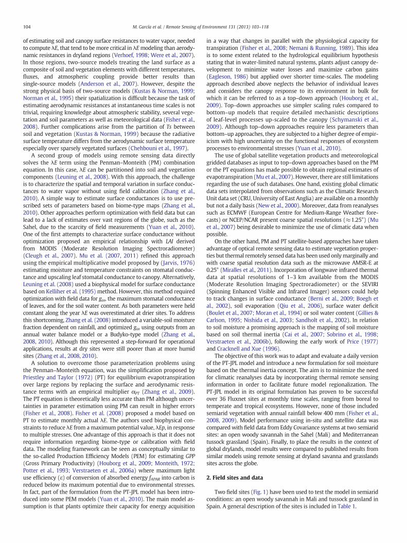
Two field sites (Fig. 1) have been used to test the model in semiaridconditions: an open woody savannah in Mali and tussock grassland inSpain. A general description of the sites is included in Table 1.

Af

Am

As

Aw

BWk

BWh

BSk

BSh

Cfa

Cfb

Cfc

Csa

Csb

Csc

Cwa

Cwb

CWc

Dfa

Dfb

Dfc

Dfd

Dsa

Dsb

Dsc

Dwa

Dwb

Dwc

Dwd

Koppen-Geiger climate classes

Balsa Blanca, Spain

Agoufou, Mali

BWh

Bsh

BSk

CSa

Aw

BSk

Am

Fig. 1. Location of the two study sites: an openwoody savanna (15.34°N, 1.48°W) in the Sahel (Agoufou site,Mali) andMediterranean tussock grassland (36.94°N, 2.03°W) in Spain (BalsaBlanca site). The map with Köppen–Geiger climate classes (Kottek et al., 2006) overlaps country boundaries. The Mediterranean site presents cold semiarid climate (BSk) and theSahelian site Arid desert hot climate (BWh).

105M. García et al. / Remote Sensing of Environment 131 (2013) 103–118

2.1. Sahelian open woody savannah site

The Agoufou site is an open woody savannah, homogeneous overseveral kilometers, with trees representing less than 5% of vegetationcover. A comprehensive description of the site is provided by Mouginet al. (2009). The top 0–6 cm of the soil is 91% sand, 3.3% silt and 4.6%clay (de Rosnay et al., 2009). The region experiences a single rainyseason with most precipitation falling between late June and midSeptember followed by a long dry season of around 8 months.

In-situ data for the 2007 growing seasonwere providedby theAfricanMonsoon Multidisciplinary Analyses (AMMA) project. Sensible heatflux was measured with sonic anemometers (CSAT) measuring thethree vector components of the wind at 20 Hz. Latent heat fluxeswere measured with the Eddy–Covariance system (Campbell CR3000and CSAT3–LiCor7500, Campbell Scientific Inc. and Li-Cor Inc.). Thefour components of the net radiation were measured with a CNR1(Kipp and Zonen CNR1, Delft, Holland).

Table 1General characteristics of the two instrumented field sites in the Sahel region and in the M

Site name(location)

Vegetation type Mean annualrainfall

Soil type D

Agoufou (Mali)(15.34°N, 1.48°W)

Open woody savannah 375 mm Fixed dunes-Arenosol CZ

Balsa Blanca (Spain)(36.94°N, 2.03°W)

Tussock grassland 370 mm Calcium crusts-Mollicleptosol

S

Measurement height for the flux sensors is 2.2 m. Soil heat fluxeswere computed from soil temperature measurements. See Timouk etal. (2009) for more details. Wind speed and direction (Vector A100R),land surface temperature (Everest 4000.4zl), air temperature andhumidity (HMP 45C, Vaisala) and precipitation (Delta T, RG1) werealso measured. Time domain reflectometry sensors (CampbellCS616, Campbell Scientific Inc., USA) measured volumetric Soil WaterContent at several depths with the shallower probe, the one used inthis work, located at 5 cm.

Leaf Area Index (LAI) and fractional cover were monitored approxi-mately every 10 days during the 2007 growing season (DOY 184 to269) along a 1 km long vegetation transect using hemispherical photo-graphs. LAI was validated using destructive measurements (Mougin etal., 2009). Comparisons with MODIS LAI during three years producedr2=0.82 and RMSE 0.26 (Mougin et al., 2009). The fraction of vegeta-tion cover is 50%, with a maximum average height of 0.4 m for the her-baceous cover. A period starting prior and finishing after the rains was

editerranean basin.

ominant herbaceous species Dominant woody species

enchrus biflorus, Aristida mutabilis,ornia glochidiata, Tragus berteronianus

Acacia raddiana, Acacia senegal,Combretum glutinosum, Balanites aegyptiaca,Leptadenia pyrotechnica

tipa tenacissima Thymus hyemalis, Chamaerops humilis L.,Brachypodium retusum (Pers.) P. Beauv,Ulex parviflorus


evaluated (DOY 170 to 315). No gap filling has been performed. Gaps influx data are present notably in late July to early August (Fig. 2).

2.2. Mediterranean grassland site

Balsa Blanca site is a tussock grassland steppe dominated by Stipatenacissima L. (91% cover) located within the “Cabo de Gata-NíjarNatural Park” (Spain) the only subdesertic protected region in Europe,with a semiarid Mediterranean climate. Annual rainfall is highly vari-able from year to year with mean values of 375 mm and mean annualtemperature of 18.1 °C. In the closer long-term station the averagewas 200 mm (records from the closest meteorological station,Nijar, distant 30 km) (Rey et al., 2012) with rainfall falling mostlyin fall and winter and a prolonged summer drought. The fraction ofvegetation cover is 60%, with mean average height of 0.7 m. The soil isclassified as Mollic Leptsol (WRB) (World Reference Base for Soil Re-sources, FAO 1998) with depth ranging from 15 to 25 cm.

In situ data were acquired during the 2011 growing season betweenJanuary and June. This period should capture most of the annual vari-ability in λE although it is only part of a complete growing season thatstarts in fall until early summer (Fig. 2). Latent and sensible heat fluxeswere measured with respective Eddy Covariance (EC) systems using athree-dimensional sonic anemometer (CSAT-3 Campbell Scientific Ltd)and an IRGA (open-path infrared gas analyzer, Li-Cor, Li-7500, CampbellScientific Ltd). The measurement heights were 3.5 m. Sensors mea-sured at 10 Hz and fluxes were estimated and stored half-hourlyapplying the corrections for axis-rotation (Kowalski et al., 1997;Mcmillen, 1988) and density fluctuations (Webb et al., 1980).

Net radiation was obtained using NR-Lite (Kipp&Zonen). Four soilheat flux plates (HFP01SC; Campbell Sci. Inc.) were placed at 8 cmdepth, two under plant and two under bare soil, and connected viamultiplexer to a datalogger. The soil heat flux at the surface was deter-mined by adding the measured heat flux at 8 cm (G) to the energystored in the layer above the heat plate estimated from soil temperatureand soil moisturemeasurements. Soil temperature wasmeasured usingsoil thermocouples (TCAV) at 2 and 6 cm depth adjacent to the heatflux plates. Land surface temperature wasmeasured with three Apogeesensors over bare soil, vegetation, and a composite of bare soil andvegetation, (IRTS-P). Air temperature and relative humidity weremeasured with thermohygrometers (HMP45C, Campbell Scientific Ltd.).Rainfall was measured using a tipping bucket rain gage of 0.25 mm ofresolution (ARG100 Campbell Scientific INC., USA). Time domain reflec-tometry sensors (CampbellCS616, Campbell Scientific Ltd) measured

0

40

80

120

SW

C (

%)

0

10

20

30

04080

120160

DOY

160 180

0.1

0.2

0.3

0.4

0.5

Savanna

Rai

n (

mm

)

λ E (

Wm

-2)

ND

VI

200 220 240 260 280 300

160 180 200 220 240 260 280 300

160 180 200 220 240 260 280 300

320

Fig. 2. Volumetric soil water content % (SWC), rainfall (mm), evapotranspiration (λE) in(Agoufou) in 2007 and in the Mediterranean grasslands (Balsa Blanca) in 2011. SWC probe

Volumetric (m3m−3) soil water content (SWC) under bare soil andunder plants with 4 cm being the top most measured soil moisture.

Fig. 2 shows the seasonal dynamics for volumetric soil water content,expressed in % (SWC), rainfall (mm), evapotranspiration (λE) in Wm−2,and NDVI for the two study sites.

2.3. Satellite data

NDVI data were acquired from the Moderate Resolution ImagingSpectroradiometer (MODIS) Terra and Acqua sensor productsMOD13Q1 and MY13Q1 (collection 5) over the two study sites. Thisproduct consists of 16-day composites of 250 m pixel (Huete et al.,2002). LAI and fPAR products from Terra and Acqua (MOD15A2,MY15A2) consisting of 8-day composites of 1 km pixel (collection 5)(Myneni et al., 2002) were acquired aswell. To get daily estimates a lin-ear interpolation using both Terra and Acqua values was performedwithin the 8-days or 16 day interval in each case.

Land Surface Temperature (LST) and broadband surface albedo (α)products used in this work were developed by the Satellite ApplicationFacility for Land Surface Analysis (LSA SAF) with data from the SpinningEnhanced Visible and Infrared Imager (SEVIRI) radiometer, onboard ofthe MSG (Meteosat Second Generation). The MSG–SEVIRI sensor in-cludes 12 separate channels and 15 min temporal resolution makingit attractive for applications requiring intra-daily information. As forany geostationary satellite the trade-off is the low spatial resolution of4.8 km at nadir (spatial sampling is 3 km) and large view angles(Schmetz et al., 2002). The LST algorithm is based on a generalizedsplit window, following (Wan & Dozier, 1996) formulation adapted toSEVIRI data (Trigo et al., 2008). It requires information on clear-skyconditions and TOA brightness temperatures for the split-windowchannels 10.8 mm and 12.0 mm. Channel and broadband emissivityare estimated as a weighted average of that of bare ground and vegeta-tion elements within each pixel using the fraction of vegetation coverderived from NDVI (Trigo et al., 2008). The albedo product is based onshortwave channels at 0.6, 0.8 and 1.6 μm. It has an effective temporalscale of 5 days and updated on a daily basis using cloud-free reflectanceobservations that are corrected for atmospheric effects using the simpli-fied radiative transfer code SMAC (Geiger et al., 2008). Dynamic infor-mation on the atmospheric pressure and total column water vaporcomes from the European Centre for Medium-rangeWeather Forecasts(ECMWF) NWP model. Cloud identification and cloud type classifica-tion are used in the processing of all LSA SAF products.

0

40

80

120

0

10

20

30

04080

120160

DOY

0.1

0.2

0.3

0.4

0.5

Mediterranean grassland R

ain

(m

m)

SW

C (

%)

λ E (

Wm

-2)

ND

VI

20 40 60 80 100 120 140 160

20 40 60 80 100 120 140 160

20 40 60 80 100 120 140 160

Wm−2, and NDVI dynamics during the periods of analyses in the Sahelian savannas were located at 5 cm and 4 cm depth respectively.


3. Methods

3.1. PT-JPL-daily model description

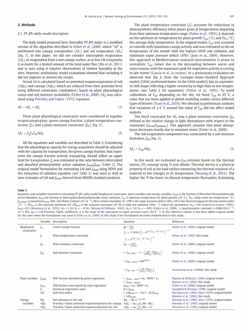
The daily model proposed here (hereafter PT-JPL-daily) is a modifiedversion of the algorithm described in Fisher et al. (2008) where “λE” ispartitioned into canopy transpiration (λEc) and soil evaporation (λEs)(Eq. 1). In this paper, we did not consider interception evaporation(λEi), or evaporation from awet canopy surface, as in low LAI ecosystemsit accounts for a limited amount of the total water flux (Mu et al., 2011)and in turn using it requires observations of relative humidity at thesites. However, preliminary model evaluations showed that including itdid not improve or worsen the results.

Actual λE is calculated based on potential evapotranspiration of soil(λEps) and canopy (λEpc) which are reduced from their potential levelusing different constraints (multipliers) based on plant physiologicalstatus and soil moisture availability (Fisher et al., 2008). λEp was calcu-lated using Priestley and Taylor (1972) equation.

λE ¼ λEc þ λEs: ð1Þ

Three plant physiological constraints were considered to regulateevapotranspiration: green canopy fraction, a plant temperature con-straint (fT) and a plant moisture constraint (fM) (Eq. 2).

λEc ¼ f gf T f MλEpc: ð2Þ

All the equations and variables are described in Table 2. Consideringthat the physiological capacity for energy acquisition should be adjustedwith the capacity for transpiration, the green canopy fraction, that repre-sents the canopy fraction actively transpiring, should reflect an upperlimit for transpiration. fgwas estimated as the ratio between interceptedand absorbed photosynthetic active radiation fAPAR/fIPAR (Table 2). Theoriginal model formulation for estimating LAI and fAPAR using NDVI andthe extinction of radiation equation (see Table 2) was used as well asnew estimates of LAI and fAPAR derived from MODIS standard products.

Table 2Equations and variables involved in estimating PT-JPL-daily model biophysical constraints, pActive Radiation, fIPAR the fraction of intercepted photosynthetically active radiation, Topt isfAPARMAX is maximum fAPAR, SWC, Soil Water Content (m3 m−3), RH is relative humidity (%), V(°C−1), ATImin is the seasonal minimum ATI, ATIMAX is the seasonal maximum ATI. Rn is dakPAR=0.5 (Brownsey et al., 1976); m1=1.16; b1=−0.14; (Myneni & Williams, 1994); m2

β=1 kPa, αPT=1.26 Priestley–Taylor coefficient; Δ is the slope of the saturation-to-vaporfor the cases when the formulation was used in Fisher et al. (2008) or this study if the form

Variable Description Equa

Biophysicalconstraints

fg Green canopy fraction fg ¼

fT Plant temperature constraintf T ¼⋅1þh

fM Plant moisture constraint fM ¼

fSM Soil moisture constraint • fS

• fSM

• f S

Plant variables fAPAR PAR fraction absorbed by green vegetation • fAP• fAP

fIPAR PAR fraction intercepted by total vegetation fIPARfc fractional vegetation cover fc=LAI Leaf Area Index • LA

• LAEnergyvariables

Rns Net radiation to the soil Rns

λEpc Priestley–Taylor potential evapotranspiration for canopy λEpcλEps Priestley–Taylor potential evapotranspiration for soil λEps

The plant temperature constraint (fT) accounts for reductions inphotosynthetic efficiency when plants grow at temperatures departingfrom their optimum temperature range (Potter et al., 1993). fT dependson the optimum air temperature for plant growth Topt (°C) and Tam (°C)the average daily temperature. In the original model, Topt was assumedto coincidewithmaximum canopy activity andwas estimated as the airtemperature of the month with the highest NDVI and radiation andminimum vapor pressure deficit (VPD) (June et al., 2004). However,this approach in Mediterranean semiarid environments is prone tounrealistic Topt values due to the decoupling between warm andrainy seasons, with themaximumpeak for vegetation activity occurringin late winter (Garcia et al., in review). In a preliminary evaluation weobserved that the fT from the Carnegie–Ames–Stanford Approachmodel (CASA) performed better. In the CASAmodel fT has an asymmet-ric bell shape reflecting a higher sensitivity to high than to low temper-atures (see Table 2 for equations) (Potter et al., 1993). To avoidcalibrations of Topt depending on the site, we fixed Topt in 25 °C, avalue that has been applied in global modeling studies across differenttypes of biomes (Yuan et al., 2010).We checked in preliminary analysesthat variations of ±5 °C around this value of Topt did not affect modeloutputs.

The third constraint for λEc was a plant moisture constraint, fM,defined as the relative change in light absorptance with respect to themaximum (fAPAR/fAPARMax). This approach assumes that plant absorp-tance decreases mostly due to moisture stress (Fisher et al., 2008).

The soil evaporation component was constrained by a soil moisturelimitation, fSM (Eq. 3).

λEs ¼ f SMλEps: ð3Þ

In this work, we evaluated an fSM estimate based on the thermalinertia (TI) concept using Ts and albedo. Thermal inertia is a physicalproperty of soil at the land surfacemeasuring the thermal response of amaterial to the changes in its temperature (Nearing et al., 2012). Thehigher the TI the lower its diurnal temperature fluctuation. Estimating

lant variables and energy variables. fAPAR is the fraction of Absorbed Photosyntheticallyoptimum temperature for plant growth (25 °C), Tam (daily mean air temperature, °C),PD is the vapor pressure deficit (kPa), ATI is the observed apparent thermal inertia indexily net radiation (Wm−2). Values for parameters: kRn=0.6 (Impens & Lemeur, 1969);=1.0; b2=−0.05 (Fisher et al., 2008), γ (psychrometric constant)=0.066 kPa C−1;pressure curve (Pa K−1). In the reference column it has been added original modelulation has been implemented in this study.

tion Reference

f APARf IPAR

Fisher et al. (2008) original model

1:1814⋅ 1þ e0:2⋅ Topt−10−Tamð Þh i−1

e0:3 −Topt−10−Tamð Þi−1Potter et al. (1993) this study

f APARf APARMax

Fisher et al. (2008) original model

M�SWC ¼ 1− SWC−SWCminSWCMax−SWCmin

� �Fisher et al. (2008) original model

−Fisher=RHVPD/β Fisher et al. (2008) original model

M−ATI ¼ ATI−ATIminATIMax−ATImin

� �Verstraeten et al. (2006b) this study

AR−NDVI=m1⋅NDVI+b1 Myneni & Williams (1994) original modelAR−MODIS Myneni et al. (2002) this study=m2⋅NDVI+b2 Fisher et al. (2008) original modelfIPAR Campbell & Norman (1998) original modelINDVI=−Ln(1− fc)/kPAR Norman et al. (1995); Ross (1976) original modelIMODIS Myneni et al. (2002) this study¼ Rn⋅e −kRnLAIð Þ Norman et al. (1995); Ross (1976) original model¼ αPT

ΔΔþγ Rn−Rnsð Þ Norman et al. (1995) original model

¼ αPTΔ

Δþγ Rns−Gð Þ Norman et al. (1995) original model

Table 3Ranges of variation for input parameters and variables in PT-JPL-daily model. For Rn, G,NDVI and Tair ranges of ±10% around monthly means and annual mean were considered.For the constant model parameters: m1, b1, m2, b2, kRn, and kPAR, the range of uncertaintywas based on values used in the literature. For the soil moisture constraint (fSM) and theplant temperature constraint (fT) a range of ±25% around the mean was considered.Description of variables and parameters can be found in Table 2.

Input var Range Reference

Tair ±10% of mean value This studyRn ±10% of mean value This studyG ±10% of mean value This studyfT ±25% of mean value This studyfSM ±25% of mean value This studyNDVI ±10% of mean value This studym1 [1.16, 1.42] This studyb1 [−0.039, −0.025] This studym2 [0.9, 1.2] Fisher et al. (2008)b2 [−0.06, −0.04] Fisher et al. (2008)kRn [0.3, 0.6] Ross (1976)kPAR [0.3, 0.6] Ross (1976)


thermal inertia requires knowing thermal conductivity of the material(K), its density (ρ) and specific heat (C) (Price, 1977).

Increasing soil moisture content modifies soil thermal conductivityand reduces the diurnal surface temperature fluctuation (Verstraetenet al., 2006b). In early studies, this diurnal Ts variation was linked theo-retically to thermal inertia resulting in the apparent thermal inertia(ATI) index (Price, 1977). Estimating thermal inertia using remote sens-ingwas first introduced by Price (1977) and expanded by Cracknell andXue (1996). Sobrino et al. (1998) and Lu et al. (2009). In this study weestimated ATI following Verstraeten et al. (2006b) which was basedon Mitra and Majumdar (2004) (see Eq. 4). ATI relies on broadbandalbedo (α), and the difference between maximum daytime (TsDMax)and minimum nighttime (TsDmin) surface temperature, and a solarcorrection factor C (Eq. 5) that normalizes for changes in solar irradi-ance with latitude, ϑ and the solar declination angle φ, the angle be-tween sun rays and the plane of the Earth's equator. It is assumed thatATI reflects both soil and canopy water content if the Ts includes bothsoil and vegetation components (Tramutoli et al., 2000; Verstraeten etal., 2006b). In fact, a composite Ts might track better changes inroot-zone SWC as the canopy temperature responds rapidly to changesin root zone SWC, which can be decoupled from the bare soil surfaceSWC. From the 15 minute Ts data the minimum (TsDmin) andmaximum(TsDMax) values from each day were extracted. Observations flagged ascloudy in the METEOSAT LST data and days when the midday observa-tion was missing were excluded from the analyses. A smoothing proce-dure averaging with the prior and following day was applied to the ATIassuming that the soil moisture conditions could be interpolated be-tween subsequent days and to remove noise.

ATI ¼ C1−α

TsDMax−TsDminð4Þ

C ¼ sinϑ sinφ⋅ 1− tan2ϑ⋅ tan2φ� �

þ cosϑ⋅ cosφ⋅ arccos − tanϑ⋅ tanφð Þ:ð5Þ

Where ϑ is latitude, and φ is solar declination estimated using themethod of Iqbal (1983).

However, the coupling between ATI and soil moisture is notstraightforward. Thermal inertia could be converted directly to soilmoisture provided that soil properties are known (Lu et al., 2009;Minacapilli et al., 2009; Van Doninck et al., 2011). Since those proper-ties only change over geologic time scales, short-term changes in ATI canbe linked to changes in soil moisture using time-series (Van Doninck etal., 2011). Verstraeten et al. (2006b) related soil moisture to remotelysensed ATI derived from METEOSAT imagery by assuming that theminimum and maximum seasonal ATI (ATImin and ATIMax) correspondto residual and saturated soil moisture contents obtaining fSM-ATI (seeequation in Table 2).

To evaluate fSM derived from ATI two additional formulations of fSMused in the original model formulation have been also tested (seeTable 2). The first is based on field measurements of Volumetric soilwater content (SWC) (fSM-SWC), where SWC was rescaled between aminimum (SWCmin) and a maximum value (SWCMax) (Fisher et al.,2008). In our case, SWCmin was estimated as the minimum value of thedry season. SWCMax was estimated as the value of SWC in the 24 h aftera strong rainfall event, which can be considered as an estimate of thefield capacity. If SWC>SWCMax then fSM-SWC=1. In the Mediterraneansite, the 2006–2011 period was used to extract SWCmin and SWCMax asthe period used to apply PT-JPL-daily was not a complete season.

The second approach to estimate fSM was the original PT-JPL modelformulation based on the link between atmospheric water deficit andsoil moisture (fSM-Fisher) (Bouchet, 1963; Morton, 1983). This link iscompromised if the vertical adjacent atmosphere is not in equilibriumwith the underlying soil (Fisher et al., 2008). The β parameter indicatesthe relative sensitivity of soil moisture to VPD (see Table 2).

3.2. Global sensitivity analyses (EFAST) approach

Sensitivity analysis can be used to evaluate the effects of uncertaintyon input or parameters on model output or to evaluate which variablesor parameters have the largest effect onmodel output (Matsushita et al.,2004). In this study Global Sensitivity Analysis (GSA) of PT-JPL-dailymodel was performed using Extended Fourier Amplitude SensitivityTest (EFAST) (Saltelli et al., 1999). EFAST was originally developed byCukier et al. (1978) and improved by Saltelli et al. (1999). The advan-tage of EFAST compared to traditional sensitivity analyses such asone-at-a-time (OAT) or experimental design (ED) is that it allowsseveral input variables to vary simultaneously considering interactionsamong them. It can be used for non-linear and non-monotonic modelsproviding similar results to more complex methods based as well onanalyses of variance but being computationally more efficient (Saltelliet al., 1999). A Fourier decomposition is used to obtain the fractionalcontribution of the individual input factors to the variance of themodel prediction (Campolongo et al., 2000).

To identify the relative importance of each model input in terms ofits contribution to the output variance of daily evapotranspiration, per-turbations for each variable were applied around the mean value of thegrowing season and also around meanmonthly values. Rn, G, NDVI andTair were varied by ±10% around their monthly means and annualmean based on reported uncertainty of field measurements for thosevariables (Garcia et al., 2008). For the constant model parameters: m1,b1, m2, b2, kRn, and kPAR, the range of uncertainty was based on valuesused in the literature (Table 3). A perturbation of ±25% around themean was considered for the soil moisture constraint (fSM) and theplant temperature constraint (fT).

3.3. Evaluation of the PT-JPL-daily evapotranspiration model

PT-JPL-daily was run using a combination of field and remotely-sensed data as inputs to parameterize the biophysical constraints andpartition the energy between soil and canopy (Table 4). Two versions(the original version and one version using MODIS products) of LAIand fAPAR were tested which modify two of the plant constraints fg,and fM as well as the energy partition between soil and vegetation(Table 2). In addition, three versions of fSM were used as explained inthe model description section (Table 2). Model results were comparedwith λE from Eddy Covariance fluxes and the coefficient of determina-tion (r2), Mean Average Error (MAE), the bias, the RMSE (Root MeanSquare Error) and MPE (Mean Absolute Percentage Error) were usedas indicators of model performance. To compare modeled λE with λEmeasurements from Eddy Covariance the energy balance from the

Table 4Eight versions of PT-JPL-daily (FD) were run based on different combinations of equations and data used for the variables: fSM, fIPAR and LAI. Rn is Net radiation (Wm−2), G is soil heatflux (Wm−2), Tair, air temperature (°C), SWC, Soil Water Content (%), VPD, Vapor pressure deficit (kPa), RH, Relative humidity (%), Ts, Surface temperature (°C), LAI (Leaf AreaIndex), fPAR (fraction of Photosynthetic Active Radiation) and α broadband surface albedo. The soil moisture constraints used were: fSM-SWC (from measured volumetric soilwater content), fSM-Fisher (from atmospheric water deficit), and fSM-ATI (from apparent thermal inertia). Two different fAPAR and LAI were used (a) fAPAR-NDVI and LAINDVI (FDamodel versions) and (b) used fAPAR-MODIS and LAIMODIS (in FDb model versions). All equations are described in Table 2.

Algorithm version Algorithm name fSM fAPAR and LAI Common variables

Estimate Data/source Estimate Data/source Data/source

1 FDaSWC fSM-SWC SWC/in situ fAPAR-NDVILAINDVI

NDVI/MODIS Rn, G, Tair/in situ NDVI/MODIS

2 FDbSWC fAPAR-MODIS

LAIMODIS

fPAR, LAI/MODIS

3 FDaFisher fSM-Fisher VPD, RH/in situ fAPAR-NDVILAINDVI

NDVI/MODIS

4 FDbFisher fAPAR-MODIS

LAIMODIS

fPAR, LAI/MODIS

5 FDaATI-in situ fSM-ATI Ts, α/in situ fAPAR-NDVILAINDVI

NDVI/MODIS

6 FDbATI-in situ fAPAR-MODIS

LAIMODIS

fPAR, LAI/MODIS

7 FDaATI-MSG Ts, α//MSG fAPAR-NDVILAINDVI

NDVI/MODIS

8 FDbATI-MSG fAPAR-MODIS

LAIMODIS

fPAR, LAI/MODIS


Eddy Covariance data should be forced to zero (Twine et al., 2000). Weused the criteria of preserving the Bowen ratio that assumes that theBowen ratio (H/λE) is well measured by the EC system and theclosure error is proportionally distributed into λE and H (Twineet al., 2000).

The evaluation results (r2, errors and biases) are presented in foursteps. First, model performance using measured soil moisture constraint(fSM-SWC) was analyzed. Here, the accuracy of the two different versionsfor LAI and fAPAR was compared as, in principle, this model version usingfSM-SWC should be themost precise from the point of view of soil moistureconstraint and can be used as a benchmark. In the second step, the feasi-bility of using fSM-Fisher, from atmospheric variables at daily time-scale insemiarid conditions was evaluated. In the third step, the performance ofthe model run with the apparent thermal inertia index fSM-ATI fromin-situ and also satellite data was evaluated. In this three steps the twoversions for estimating LAI and fAPAR were evaluated as well resulting ina total of eight algorithm versions evaluated (see Table 4). Finally, toplacemodel results in the context of global drylands, our accuracy resultswere compared to published accuracy results from other models thatused remote sensing information at the same and at other drylandsavanna and grasslands sites across the globe. In those cases whenmodel outputs were provided by the authors at 30 minutes timestep, they where aggregated at daily time scale and compared withthe Eddy Covariance data to have comparable statistics.

4. Results and discussion

4.1. Global sensitivity analyses (EFAST) approach

Considering the variability around mean annual conditions, thecontribution to uncertainty was less than 20% for most parametersand variables in the Sahelian savanna. The greatest uncertainty wasdue to two of the biophysical constraints: fSM and fT with 22.19%and 17.68% respectively (total effect). Five other variables involvedin LAI estimation and energy partition between soil and canopy contrib-uted around 12% to model uncertainty (Fig. 3). However, the relativeimportance of each variable depends on the time of the year. At the be-ginning of the season, λEwasmost sensitive to accuracy in fSM reachingthe maximum value of explained variance among all variables andmonths (40%). During the maximum peak of NDVI, in the middle ofthe season, the greatest sensitivity was due to fT, and m1 (involved in

fM and fg estimates via fAPAR). During the senescent phase, the modelwas more sensitive to accuracy in kPAR and kRn, involved in energypartition into soil and vegetation.

Under annual Mediterranean conditions, most of the uncertaintywas related to the partition of energy between soil and vegetation,shown by the highest sensitivity to the two coefficients of extinctionof radiation: kPAR (50%) involved in LAI estimates, and kRn (20%) bothcontributing to estimate the net radiation reaching the soil component.This is similar to the situation during the senescent phase in the Sahel.Seasonally, the relative importance of each variable was similar to theannual pattern, except in January whenmodeled λEwasmore sensitiveto accuracy in Rn.

Fig. 3 shows how in both ecosystem types, mean effect and totaleffect (that considers interactions) on evapotranspiration were verysimilar with differences around 1–2%, indicating low effect of variableinteractions.

4.2. Evaluation of the PT-JPL-daily evapotranspiration model with EddyCovariance data

4.2.1. Soil moisture constraint from measured soil moisture (fSM-SWC)In the Sahelian savanna the performance of PT-JPL-daily λE

model using measured SWC (fSM-SWC) was similar regardless of thefAPAR and LAI estimate used (FDaSWC or FDbSWC) (r2=0.85–0.86 andMAE=14.14–13.54) (Table 5 and Fig. 4a, b). In the Mediterraneangrasslands, both the coefficient of determination and errors werealso similar regardless of the fAPAR and LAI used (r2=0.75–0.74;MAE=10.66–11.44) (Table 5 and Fig. 5a, b). Therefore, PT-JPL-daily for-mulation is capable to reproduce thedynamics ofλE in theMediterraneangrasslands, as it explained75%of theλE variance. Considering that the un-certainty of the energy balance closure from Eddy Covariance data in thisMediterranean site, calculated at daily time scale, represents 21.7% of theavailable energy (Rn-G), the accuracy obtained with PT-JPL-daily usingfSM-SWC is closest to the one from Eddy Covariance. In the Sahel, themodel explains up to 86% of the variance, which considering that theclosure error is 5.78% of the available energy at daily scale is also closeto the instrumental accuracy. However, in this site during the growingseason there was a systematic underestimate of λE during the periodof maximum growth followed by an overestimate, independently ofthe fAPAR and LAI used (Fig. 4a and b).

Mediterranean grasslands

Main Effect

Total Effect

Sahelian savanna

0

20

40

60

Tair Rn G

% v

aria

nce

Main Effect

Total Effect

Tair

Rn

NDVI

G

fSM

fT

kRn

kPAR

m1

b1

m2

b20

20

40

60

Jan JunJun Jul Aug Nov

% v

aria

nce

Tair

Rn

NDVI

G

fSM

fT

kRn

kpar

m1

b1

m2

b2Sep Oct Feb Mar Apr May

NDVI fSM fT kRn kPAR m1 b1 m2 b2 Tair Rn GNDVI fSM fT kRn kPAR m1 b1 m2 b2

Fig. 3. Upper panels: sensitivity of modeled evapotranspiration according to mean annual conditions (% percentage of explained variance). Main effect is the variance explainedwithout considering interactions among variables and total effect considering interactions. Lower panels: sensitivity of modeled evapotranspiration considering monthly conditionsin the Sahelian savanna and Mediterranean grasslands (total effect). Uncertainty levels were set as ±10% of the mean for input variables NDVI, Tam, Rn, and G and of ±25% of themean for the soil moisture (fSM) and plant temperature (fT) constraints. For constant model parameters: m1, b1, m2, b2, kRn, and kPAR, the range of uncertainty was based on valuesused in the literature.


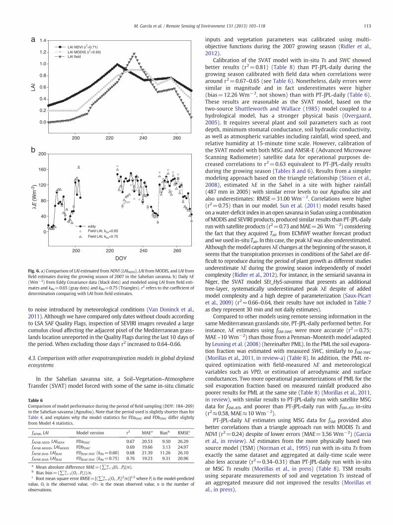
To assess whether this mismatch in the Sahelian site could be relatedto the LAI and fPAR estimates, we compared satellite LAI estimates withfield estimates and also evaluated the evapotranspiration model ranwith field estimates for LAI and fPAR. Comparison of LAI satellite productswith field estimates (Fig. 6a) showed better correlations with MODIS

Table 5Evaluation of PT-JPL-daily λE with Eddy Covariance data. In the savanna the resultshave been evaluated between June and December 2007 and in the Mediterraneangrasslands between January and June 2011. Model versions starting with “FDa” wererun with fAPAR-NDVI and LAINDVI and with “FDb” with fAPAR-MODIS and LAIMODIS. fSM-SWC isthe soil moisture constraint derived from measured volumetric soil water content, andfSM-ATI from apparent thermal inertia. Surface temperature and albedo could be acquiredfrom in-situ sensors or from satellite (MSG) sensors.

Site fSM Modelversion

r2 MAEa Biasb RMSEc MAPD(%)d

Sahelian savanna(all dates)

In-situ FDaSWC 0.85 14.14 7.59 21.45 22.69FDbSWC 0.86 13.54 4.02 20.39 21.72FDaATI-in situ 0.82 20.69 −1.48 23.88 33.20

Satellite FDbATI-in situ 0.83 19.72 −7.14 23.10 31.65FDaATI-MSG 0.79 23.11 16.52 30.55 37.09FDbATI-MSG 0.80 20.21 11.78 26.53 32.43

Mediterraneangrasslands(growing season)

In-situ FDaSWC 0.75 10.66 10.10 12.43 30.89FDbSWC 0.74 11.44 10.96 13.2 33.16FDaATI-in situ 0.58 9.66 5.70 11.10 28.01

Satellite FDbATI-in situ 0.57 9.85 6.21 11.58 28.57FDaATI-MSG 0.32 10.16 −3.01 14.48 29.46FDbATI-MSG 0.31 10.78 −3.80 15.03 31.26

a Mean absolute difference MAE=(∑i=1n |Oi−Pi|/n).

b Bias bias=(∑i=1n (Oi−Pi))/n.

c Root mean square error RMSE=[(∑i=1n (Oi−Pi)2/n)]1/2.

d Mean absolute percentage difference MAPE ¼ 100bO> ∑n

i¼1 Oi−Pij j=n� �, where Pi is the

model-predicted value, Oi is the observed value, bO> is the mean observed value, n isthe number of observations.

LAI (r2=0.93) than for LAI estimated from NDVI (r2=0.71). AlthoughMODIS LAI underestimated the maximum peak and overestimated LAIduring growing and senescence stages its phenology pattern matchedbetter with the field data than the LAI derived from NDVI (Fig. 6a). Inthis case, the maximum LAI happened earlier in the season than thefieldmaximum LAI, showing also greater overestimates during growingand senescent phases. This could explain a slightly better performanceof the λE model using MODIS products during the growing season(Table 6).

However, model outputs ran using field measured LAI, fc and fAPAR(estimated as described in Mougin et al., 2009) did not improvemodel performance (see Table 6). Therefore, using satellite productsfor vegetation (LAI and fPAR) to run the model produce similar resultsthan using field vegetation estimates.

It seems that when vegetation is changing very rapidly around theseasonal peak in the Sahel, the model can account for the generalpattern of λE but not for minor ups and downs observed in theEddy Covariance λE. Increasing the energy partition allocated to vegeta-tion by using kRn of 0.75, a value obtained by optimization at the site(Ridler et al., 2012), improved significantly the results (r2=0.76 vs r2=0.68) (Table 6). Using this coefficient reduced the λE offset after the LAIpeak, but not before (Fig. 6b). It should be noted that field LAI estimates(Fig. 7) present uncertainty as well, as they were interpolated betweenthefield samplings, acquired every≈10 days. Thus, before themaximumLAI peak (DOY=235) the previous field sampling was 10 days earlier,making it possible to miss a higher and earlier maximum peak. In thatcase, LAI underestimates would produce λE underestimates betweenthe periods DOY225 and DOY235 (Fig. 6).

These results suggest that themodel could benefit froman improvedenergy partitioning between soil and canopy considering variable ex-tinction coefficients and separate longwave and shortwave components(Kustas & Norman, 1999), as well as from shorter-time scale estimatesof LAI and fPAR.

DOY160 180 200 220 240 260 280 300

λE (

Wm

-2)

0

50

100

150

200

DOY160 180 200 220 240 260 280 300

0

50

100

150

200

160 180 200 220 240 260 280 300

0

50

100

150

200

160 180 200 220 240 260 280 300

0

50

100

150

200

160 180 200 220 240 260 280 300

0

50

100

150

200

160 180 200 220 240 260 280 300

λE(W

m-2

)

0

50

100

150

200

fSM-SWC

fSM-Fisher

fSM-ATI-in situ

fSM-ATI-MSG

fAPAR-NDVI ; LAINDVI fAPAR-MODIS ; LAIMODIS

160 180 200 220 240 260 280 300

λE (

Wm

-2)

0

50

100

150

200

160 180 200 220 240 260 280 300

0

50

100

150

200

g

e

c

a

h

f

d

b

λE (

Wm

-2)

Fig. 4. Daily λE (Wm−2) in the Sahelian savanna (Agoufou, Mali) from Eddy Covariance data (black dots) andmodeled (white dots) during 2007. In the first column (figures a, c, e, g) themodel was run using fAPAR-NDVI and LAINDVI and in the second column (figures b, d, f, h) using fAPAR-MODIS and LAIMODIS. In each of the six rows, the model was run a different soil moistureconstraint: fSM-SWC frommeasured volumetric soil water content (figures a, b), fSM-Fisher from atmosphericwater deficit (figures c, d), fSM-ATIin-situ from apparent thermal inertia from in-situmeasurements (figures e, f), fSM-ATI-MSG from apparent thermal inertia from MSG–SEVIRI measurements (figures g, h).


4.2.2. Soil moisture constraint from atmospheric variables (fSM-Fisher)Estimating λE using fSM-Fisher with the same parameterization as in

Fisher et al. (2008) (β=1; midday conditions) did not provide mean-ingful results in the Mediterranean grasslands (r2~0.16) (Table 7). Inthe savanna, correlations were better but well below those found forfSM-SWC (r2=0.61–0.62) and with high biases around 25–29 Wm−2

(Table 4, Figs. 5 and 6). This constraint diagnosed the major waterstress during the growing season around DOYs 240–250. We evalu-ated the sensitivity of fSM-Fisher to β values between 0.05 and 2, andto the use of daily average or midday conditions for RH and VPD.Table 7 shows the results when themodel was runwith two differentvalues of β. They are shown in the table as they provided the best re-sults in each site: β=0.1 kPa, that was applied at a global scale in Muet al. (2007), and β=1 kPa applied in Fisher et al. (2008).

In the savanna, the best results corresponded to β=1 kPa anddaily average conditions (r2=0.80; MAE=18.08 Wm−2). In theMediterranean grasslands PT-JPL-daily performed better using β=0.1(Table 7), especially for midday conditions (r2=0.64–0.53) although

λE was systematically underestimated (biases≈15–17 Wm−2). Theseresults suggest a stronger control of atmospheric conditions on soilmoisture changes in the Mediterranean conditions than in the Sahel.Therefore, parameterization using fSM-Fisher should be tuned accordingto the conditions in each site for successful results.

4.2.3. Soil moisture constraint from apparent thermal inertia (fSM-ATI)Using in-situ data, model performance in the savanna for the thermal

inertia index fSM-ATIwaspractically equivalent to that using SWC (fSM-SWC),with r2≈0.82 and slightly higher errors but similar or lower biases(Table 5). Non significant differences were found when using fAPAR andLAI from MODIS or a linear function of NDVI except from a slightlylower biaswith the latter. At the endof the rainy season (DOY270), fSM-ATI

overestimated λE as even at an entirely dry soil the ATI index will neverbecome zero, since that would require an infinite temperature amplitude(Van Doninck et al., 2011).

In the Mediterranean grasslands, statistics frommodel performanceusing fSM-ATI from in-situ data were again not as good as than in the

0 20 40 60 80 100 120 140 160 180

0

40

80

120

0 20 40 60 80 100 120 140 160 180

λE (

Wm

-2)

0

40

80

120

fSM-SWC

fSM-Fisher

fSM-ATI-in situ

fSM-ATI-MSG

fAPAR-NDVI ; LAINDVI fAPAR-MODIS ; LAIMODIS

0 20 40 60 80 100 120 140 160 180

0

40

80

120

0 20 40 60 80 100 120 140 160 180

λE (

Wm

-2)

0

40

80

120

0 20 40 60 80 100 120 140 160 180

0

40

80

120

0 20 40 60 80 100 120 140 160 180

λE (

Wm

-2)

0

40

80

120

0 20 40 60 80 100 120 140 160 180

0

40

80

120

0 20 40 60 80 100 120 140 160 180

λE (

Wm

-2)

0

20

40

60

80

100

120

hg

fe

dc

a b

DOY DOY

Fig. 5. Daily λE (Wm−2) in the Mediterranean grassland (Balsa Blanca, Spain) from Eddy Covariance data (black dots) and modeled (white dots) during 2007. In the first column(figures a, c, e, g) the model was run using fAPAR-NDVI and LAINDVI and in the second column (figures b, d, f, h) using fAPAR-MODIS and LAIMODIS. In each of the six rows, the model was runa different soil moisture constraint: fSM-SWC from measured volumetric soil water content (figures a, b), fSM-Fisher from atmospheric water deficit (figures c, d), fSM-ATIin-situ from ap-parent thermal inertia from in-situ measurements (figures e, f), fSM-ATI-MSG from apparent thermal inertia from MSG–SEVIRI measurements (figures g, h).


savanna. Although the r2 using fSM-ATIwas lower than those obtainedwithfSM-SWC, the errors decreased and the biases were half of those obtainedwith fSM-SWC. Similar to the savanna site, results were quite similar inde-pendently of the LAI and fPAR estimate used to run the model.

When running the model using satellite MSG instead of in-situdata for fSM-ATI, good results were obtained in the savanna site interms of r2 ~0.80 and MAE=23.1–20.1 Wm−2 (Table 5) but higherbiases were detected due to λE underestimates during the growing sea-son (Fig. 4g, h). This was due to the fact that the diurnal Ts difference(TsDMax−TsDmin) was always higher for MSG than for in-situ data(Fig. 7), producing lower soil moisture (fSM) values.

In the Mediterranean grasslands, using MSG data instead of in-situto estimate fSM-ATI produced a greater loss of accuracy in r2 than in thesavanna although errors were similar and biases even lower than within-situ data (Table 5). On one hand, results using in-situ data wereworse to start with than in the savanna with correlations aroundr2=0.58. As in the Mediterranean site λE is lower (Fig. 2) themodel is less tolerant to different error sources. Besides the noise appar-ent in the MSG time-series, the comparability of the diurnal temperature

difference (TsDMax−TsDmin) between in situ and MSG data was moreproblematic than in the savanna, with systematically higher MSG values(Fig. 7). Additional inspection of Ts (15 min) observations between fieldand satellite (Fig. 8) showed that differences between in-situ and satellitewere larger in the grasslands (MAE=2.43 °C) than in the savanna(MAE=1.56 °C). In the Mediterranean site the sensor viewing angle is42.68° while in the Sahel it is only 18.01°. This results in a larger scalemismatch at the Mediterranean site between the satellite pixel and thefootprint of the in-situ sensors as well as greater atmospheric effectsdue to a larger atmospheric path radiance.

The fSM-ATI approach is very sensitive to uncertainty in thermal datasince day and night Ts are used in the denominator (Cai et al., 2007;Sobrino et al., 1998; Verstraeten et al., 2006b). Sensitivity to errors isgreater when Rn is higher which occurs at the end of the study periodin the Mediterranean site and the middle of the season in the Saheliansite (Guichard et al., 2009) (see Figs. 4g, h and 5g, h). In fact, in theMediterranean grasslands, the lack of fit for fSM-ATI MSG (r2=0.32–0.31)was caused by the last 10 days of the study period (see Fig. 5g and h).Another important limitation of the ATImethodology is the vulnerability

LAI

0.0

0.2

0.4

0.6

0.8

1.0

1.2

1.4LAI NDVI (r

2=0.71)

LAI MODIS (r2=0.93)

LAI field

DOY

200 220 240 260

200 220 240 260

λE (

Wm

-2)

0

40

80

120

160

200

eddyField LAI; kRn=0.65

Field LAI; kRn=0.75

a

b

Fig. 6. a) Comparison of LAI estimated from NDVI (LAINDVI), LAI fromMODIS, and LAI fromfield estimates during the growing season of 2007 in the Sahelian savanna. b) Daily λE(Wm−2) from Eddy Covariance data (black dots) and modeled using LAI from field esti-mates and kRn=0.65 (gray dots) and kRn=0.75 (Triangles). r2 refers to the coefficient ofdetermination comparing with LAI from field estimates.


to noise introduced by meteorological conditions (Van Doninck et al.,2011). Althoughwe have compared only dates without clouds accordingto LSA SAF Quality Flags, inspection of SEVIRI images revealed a largecumulus cloud affecting the adjacent pixel of the Mediterranean grass-lands location unreported in the Quality Flags during the last 10 days ofthe period. When excluding those days r2 increased to 0.64–0.66.

4.3. Comparison with other evapotranspiration models in global drylandecosystems

In the Sahelian savanna site, a Soil–Vegetation–AtmosphereTransfer (SVAT) model forced with some of the same in-situ climatic

Table 6Comparison of model performance during the period of field sampling (DOY: 184–269)in the Sahelian savanna (Agoufou). Note that the period used is slightly shorter than forTable 4, and explains why the model statistics for FDaSWC and FDbSWC differ slightlyfrom Model 4 statistics.

fAPAR, LAI Model version r2 MAEa Biasb RMSEc

fAPAR-NDVI, LAINDVI FDaSWC 0.67 20.53 9.50 26.29fAPAR-MODIS, LAIMODIS FDbSWC 0.69 19.66 3.13 24.97fAPAR-field, LAIfield FDfield-SWC (kRn=0.60) 0.68 21.39 11.26 26.10fAPAR-field, LAIfield FDfield-SWC (kRn=0.75) 0.76 19.23 9.31 20.96

a Mean absolute difference MAE=(∑i=1n |Oi−Pi|/n).

b Bias bias=(∑i=1n (Oi−Pi))/n.

c Root mean square error RMSE=[(∑i=1n (Oi−Pi)2/n)]1/2 where Pi is the model-predicted

value, Oi is the observed value, bO> is the mean observed value, n is the number ofobservations.

inputs and vegetation parameters was calibrated using multi-objective functions during the 2007 growing season (Ridler et al.,2012).

Calibration of the SVAT model with in-situ Ts and SWC showedbetter results (r2=0.81) (Table 8) than PT-JPL-daily during thegrowing season calibrated with field data when correlations werearound r2=0.67–0.65 (see Table 6). Nonetheless, daily errors weresimilar in magnitude and in fact underestimates were higher(bias=12.26 Wm−2, not shown) than with PT-JPL-daily (Table 6).These results are reasonable as the SVAT model, based on thetwo-source Shuttleworth and Wallace (1985) model coupled to ahydrological model, has a stronger physical basis (Overgaard,2005). It requires several plant and soil parameters such as rootdepth, minimum stomatal conductance, soil hydraulic conductivity,as well as atmospheric variables including rainfall, wind speed, andrelative humidity at 15-minute time scale. However, calibration ofthe SVAT model with both MSG and AMSR-E (Advanced MicrowaveScanning Radiometer) satellite data for operational purposes de-creased correlations to r2=0.63 equivalent to PT-JPL-daily resultsduring the growing season (Tables 8 and 6). Results from a simplermodeling approach based on the triangle relationship (Stisen et al.,2008), estimated λE in the Sahel in a site with higher rainfall(487 mm in 2005) with similar error levels to our Agoufou site andalso underestimates: RMSE=31.00 Wm−2. Correlations were higher(r2=0.75) than in our model. Sun et al. (2011) model results basedon awater-deficit index in an open savanna in Sudanusing a combinationofMODIS and SEVIRI products, produced similar results than PT-JPL-dailyrunwith satellite products (r2=0.73 andMAE=26 Wm−2) consideringthe fact that they acquired Tair from ECMWF weather forecast productandweused in-situ Tair. In this case, thepeakλEwas also underestimated.Although themodel capturesλE changes at the beginning of the season, itseems that the transpiration processes in conditions of the Sahel are dif-ficult to reproduce during the period of plant growth as different studiesunderestimate λE during the growing season independently of modelcomplexity (Ridler et al., 2012). For instance, in the semiarid savanna inNiger, the SVAT model SEt_HyS-savanna that presents an additionaltree-layer, systematically underestimated peak λE despite of addedmodel complexity and a high degree of parameterization (Saux-Picartet al., 2009) (r2=0.66–0.64, their results have not included in Table 7as they represent 30 min and not daily estimates).

Compared to other models using remote sensing information in thesameMediterranean grasslands site, PT-JPL-daily performed better. Forinstance, λE estimates using fSM-SWC were more accurate (r2=0.75;MAE ~10 Wm−2) than those from a Penman–Monteithmodel adaptedby Leuning et al. (2008) (hereinafter PML). In the PML the soil evapora-tion fraction was estimated with measured SWC, similarly to fSM-SWC

(Morillas et al., 2011, in review-a) (Table 8). In addition, the PML re-quired optimization with field-measured λE and meteorologicalvariables such as VPD, or estimation of aerodynamic and surfaceconductances. Two more operational parameterizations of PML for thesoil evaporation fraction based on measured rainfall produced alsopoorer results for PML at the same site (Table 8) (Morillas et al., 2011,in review), with similar results to PT-JPL-daily run with satellite MSGdata for fSM-ATI, and poorer than PT-JPL-daily run with fSM-ATI in-situ(r2≈0.58, MAE≈10 Wm−2).

PT-JPL-daily λE estimates using MSG data for fSM provided alsobetter correlations than a triangle approach run with MODIS Ts andNDVI (r2=0.24) despite of lower errors (MAE=3.56 Wm−2) (Garciaet al., in review). λE estimates from the more physically based twosource model (TSM) (Norman et al., 1995) run with in-situ Ts fromexactly the same dataset and aggregated at daily-time scale werealso less accurate (r2=0.34–0.31) than PT-JPL-daily run with in-situor MSG Ts results (Morillas et al., in press) (Table 8). TSM resultsusing separate measurements of soil and vegetation Ts instead ofan aggregated measure did not improved the results (Morillas etal., in press).

0

5

10

15

20

25

30

0 5 10 15 20 25 3010 20 30 40

10

20

30

40 ssarGannavaS

Field Ts (oC) Field Ts (oC)

MS

G T

s (o

C)

Ts DMAX-Ts Dmin Ts DMAX-Ts Dmin

Fig. 7. Comparison of the diurnal surface temperature difference (TsDMAX−TsDmin) from field (Apogee) and satellite (MSG–SEVIRI) sensors in the savanna and in the Mediterraneangrassland.


Finally, to place the results from PT-JPL-daily ran with ATI in thecontext of global drylands, we compared them with studies usingPenman–Monteith remote sensing (PM) or Priestley–Taylor (PT)models over savannas and grasslands at dryland sites from differentregions of the globe (Table 8). These comparisons should always beconsidered with caution as each model uses different input datasources and both the environmental conditions and the vegetationchange. However, we have focused on the less accurate PT-JPL-dailyalgorithm, amenable for regionalization (FDaATI-MSG) ran with satelliteMSG andMODIS data both for vegetation and soil moisture constraints,leaving Tair and available energy as the only field input variablesused.

It can be seen in Table 8 that PT-JPL-daily FDaATI-MSG in the Saheliansavanna (r2=0.80; RMSE=26.53 Wm−2) performed better in generalthan PMmodels at other savanna sites although it has to be consideredthat not all these models were forced with local meteorological inputs(Table 8). Thus, the PML improved algorithm from Zhang et al. (2010)where maximum stomatal conductance is optimized with a hydro-meteorological model, showed lower r2 at two Australian savannas(r2=0.53 and 0.49) less arid than our site (with 1764 mm and526 mm of annual rainfall respectively) with the PT-JPL-daily errorwithin the range of those two sites (Table 8). Results from a PM

Table 7Evaluation of PT-JPL-daily λE with Eddy Covariance data for different parameterizations of thResults are shown for midday and daily average conditions for RH (relative humidity) andperforming combination of parameters in each site are shown in bold font. In the savanna resulfrom January to June 2011. Model versions starting with “FDa” were run with fAPAR-NDVI and LA

Site Period Conditions β (k

Savanna (Agoufou) All dates daily 1

0.1

Midday 1

0.1

Mediterranean grasslands (Balsa Blanca) Growing season Daily 1

0.1

Midday 1

0.1

model in one of theAustralian savannas forcedwith in-situmeteorolog-ical inputs were also poorer than our results (r2=0.23) (Cleugh et al.,2007). Our algorithm performed also better than the MODIS productfor evapotranspiration (MOD16) of Mu et al. (2011), in threewoody savannas in arid regions of the USA (with r2 ranging from 0.06to 0.61). Again, PT-JPL-daily errors were within Mu et al. (2011) rangesof error at those savanna sites (RMSE=18.51–30.6 Wm−2). In anotherglobal study Yuan et al. (2010) used a PM approach optimized withEddy Covariance λE from 21 sites. Their model in the Mediterraneansavanna of Tonzi performed worse (Table 8) than PT-JPL-daily usingfSM-ATI MSG in the Sahelian savannah although it should be noted thatthey used air temperature from reanalysis. In the same savanna ofTonzi ranch, Vinukollu et al. (2011) applied a daily version of thePT-JPL model with the soil moisture constraint based on the watervapor deficit although the error was low (RMSE=18.75 Wm−2) thenon-parametric Kendall's Tau (equivalent to Pearson-correlation coeffi-cient) was 0.74 using only satellite input data.

Regarding the Mediterranean grassland site, our model λE resultsusing satellite data for soil moisture and vegetation (FDaATI-MSG)(r2=0.32; RMSE=15.03 Wm−2) were in the range of the MOD16algorithm of Mu et al. (2011) for two arid steppe grasslands in theUSA with r2=0.48 (Audubon) and 0.25 (Walnut Gulch) respectively

e soil moisture constraint derived from atmospheric water deficit: fSM−Fisher=RHVPD/β.VPD (Vapor Pressure Deficit) and for β=0.1 kPa and β=1 kPa. Results from the bestts were evaluated between June and December 2007 and in theMediterranean grasslandsINDVI and with “FDb” with fAPAR-MODIS and LAIMODIS.

Pa) Model version r2 MAE Bias RMSE MPE (%)

FDaFisher 0.69 26.09 14.87 32.81 41.87FDbFisher 0.80 18.08 8.47 24.35 29.01FDaFisher 0.71 20.49 41.13 53.18 32.88FDbFisher 0.66 23.60 37.92 49.94 37.87FDaFisher 0.62 32.19 29.27 43.05 51.65FDbFisher 0.61 35.72 25.62 40.61 57.32FDaFisher 0.68 18.65 43.04 56.21 29.93FDbFisher 0.65 21.86 39.71 52.45 35.09FDaFisher 0.16 15.08 −6.68 19.40 43.73FDbFisher 0.17 28.25 −26.38 34.44 81.89FDaFisher 0.36 21.22 8.49 14.74 66.67FDbFisher 0.27 20.40 9.49 16.24 64.10FDaFisher 0.16 35.03 −7.02 20.48 110.05FDbFisher 0.13 36.24 −8.23 21.92 113.87FDaFisher 0.64 14.42 15.61 18.23 45.30FDbFisher 0.53 12.24 17.92 20.66 38.44

0 10 20 30 40 50 60 0 10 20 30 40 50 60

Field Ts (oC) Field Ts (oC)

0

10

20

30

40

50

60

MS

G T

s (o

C)

MS

G T

s (o

C)

r2 = 0.86; MAE=1.56 °C; bias=-0.42°C

0

10

20

30

40

50

60

r2 = 0.88; MAE=2.43 °C; bias=1.44°C

Savanna Mediterraneangrassland

Fig. 8. Comparison of 15 minute observations of radiometric surface temperature from field (Apogee) and satellite (MSG–SEVIRI) sensors in the savanna and in the Mediterraneangrassland during the study period.

Table 8Statistics from actual evapotranspiration models using remote sensing data over dryland savanna and grassland sites. Climate classification is based on Köppen–Geiger (Kottek etal., 2006) where BWh: arid/desert/hot air; BSk: cold/semiarid, Aw: equatorial/desert; Csb: warm temperate/summer dry/warm summer; Cfb: warm temperate/fully humid/warmsummer; Csa: warm temperate/summer dry/hot summer. A brief description of model type is included. When errors were reported in mm day−1 they have been converted intoWm−2. Statistics in parenthesis refer to the model type explanations in parenthesis.

Ecosystemtype

Site Country Lat°Lon°

Climatetype

Model type r2 MAE RMSE Reference

Open woodysavanna

Sahel (Agoufou) Mali 15.34, −1.48 BWh PT-JPL-daily fSM-ATI

satellite (in-situ)0.80 (0.83) 20.21

(19.72)26.53(23.10)

This study

Open woodysavanna

Sahel (Agoufou) Mali 15.34, −1.48 BWh SVAT in-situ calibration 0.81 16.57 9.90 Ridler et al. (2012)a

Open woodysavanna

Sahel (Agoufou) Mali 15.34, −1.48 BWh SVAT satellite calibration 0.63 39.24 46.66 Ridler et al. (2012)a

Open woodysavanna

Sahel (Dahra) Senegal 15.41 −15.47 BWh Triangle usingSEVIRI/MODIS

0.75 – 31.00 Stisen et al. (2008)

Open woodysavanna

Sahel (SD-DEM) Sudan 13.28 −0.48 BWh Sim-ReSET usingSEVIRI/MODIS

0.73 26.00 – Sun et al. (2011)

Open woodysavanna

Virginia Park Australia −19.88 146.55 Aw PM- in situ meteorological 0.23 – 112.1 Cleugh et al. (2007)

Open woodysavanna

Virginia Park Australia −19.88 146.55 Aw PML-optimizedwith hydrol. model

0.49 – 15.94 Zhang et al. (2010)

Savanna Howard Springs Australia −12.50° 131.15 Aw PML-optimizedwith hydro. model

0.53 – 32.18 Zhang et al. (2010)

Woody savanna AZ - Flagstaff - Wildfire USA 35.40−111.80 Csb MOD16. PM newversion (old version)

0.06 (0.42) – 23.92(18.51)

Mu et al. (2011)

Woody savanna TX -Freeman RanchMesquite Juniper

USA 29.9 − 98.0 Cfa MOD16. PM newversion (old version)

0.48 (0.52) – 25.91(30.76)

Mu et al. (2011)

Mediterraneansavanna

CA - Tonzi Ranch USA 38.4 − 121.0 Csa MOD16. PM new version(old version)

0.61 (0.53) – 19.08(21.36)

Mu et al. (2011)


CA - Tonzi Ranch USA 38.4 − 121.0 Csa PM (field eddy calibration) 0.57 – 30.19 Yuan et al. (2010)


CA - Tonzi Ranch USA 38.4 Csa PT-JPL-daily 0.74 (Kendall) 19.39 Vinukollu et al. (2011)

Mediterraneangrasslands

Balsa Blanca Spain 36.94 −2.03 BSk PT-JPL-daily fSM-ATI

satellite (in-situ)0.31 (0.57) 10.78

(11.44)15.03(10.96)

This study


Balsa Blanca Spain 36.94 −2.03 BSk PML-input SWC 0.54 13.03 – Morillas et al. (2011),in review


Balsa Blanca Spain 36.94 −2.03 BSk PML-input rainfall(two methods)

0.32–0.47 13.88–9.92 – Morillas et al. (2011),in review


Balsa Blanca Spain 36.94 −2.03 BSk Triangle using MODIS 0.24 3.56 – Garcia et al. (in review)


Balsa Blanca Spain 36.94 −2.03 BSk TSM with Ts compositein parallel (series)

0.34 (0.31) 39.05(53.82)

43.89(58.52)

Morillas et al. (in press)a


Balsa Blanca Spain 36.94 −2.03 BSk TSM with Ts soil,Ts canopy in parallel (series)

0.14 (0.25) 44.86(57.67)

51.00(62.50)

Morillas et al. (in press)a

Arid steppegrasslands

AZ -AudubonResearch Ranch

USA 31.6 −110.5 BSk MOD16. PM newversion (old version)

0.22 (0.48) – 23.07(23.07)

Mu et al. (2011)


AZ -AudubonResearch Ranch

USA 31.6 −110.5 BSk PT-JPL-daily 0.37(Kendall's)

18.75 Vinukollu et al. (2011)


AZ - Walnut GulchKendall Grasslands

USA 31.7 −109.9 BSk MOD16. PM newversion (old version)

0.07 (0.25) – 19.36(18.51)

Mu et al. (2011)

Mediterraneangrassland

CA-Vairaranch USA 38.40 −120.95 Csa PM (field eddy calibration) 0.51 – −4.56 Yuan et al. (2010)

a 30 minute model outputs provided by the authors have been aggregated to daily time scale in this work to compare with the rest of the models.



with the old algorithm version and r2=0.05 and 0.49 with the newversion. Our PT-JPL-daily model errors were lower than Mu et al.(2011); RMSE=22.95 and 18.42 Wm−2 with the old algorithm andRMSE=22.95 and 19.26 Wm−2 with the new algorithm. In Audubonsteppe the PT-JPL-daily model of Vinukollu et al. (2011) was not verysuccessful in capturing the temporal dynamics (Kendall's Tau=0.37)but showed still a better performance than Mu et al. (2011) algorithmran during the same time (not shown in Table 8). Results from Yuan etal. (2010) PMmodel calibrated with field data at another Mediterraneangrassland (Vairaranch) were better than our model results r2=0.51 andbias=0.16 Wm−2.

5. Conclusions

The Priestley Taylor-Jet Propulsion Laboratory (PT-JPL) evapo-transpiration λE model, developed by Fisher et al. (2008) is basedon the Priestley–Taylor equation downscaled according to multiplestresses. The PT-JPL is attractive for its simplicity and potential for re-gionalization using satellite data. In this study, a daily version of themodel was evaluated in some of the most extreme conditions fromthe point of water availability: an open woody savanna in the Saheland a Mediterranean grassland, both with annual rainfall below400 mm. A new approach was tested with in-situ and satellite datausing a soil moisture constraint based on the apparent thermal inertiaconcept (fSM-ATI) relying on remotely sensed observations of surfacetemperature and albedo.

When using field measured soil water content (SWC) to estimatethe soil moisture constraint, the daily PT-JPL model reproduced theλE dynamicsmeasured from Eddy Covariance systemswithin the un-certainty levels of the closure error system. When using the apparentthermal inertia index fSM-ATI at the Sahelian savanna, results within-situ data were equivalent to those obtained using field measuredSWC. When up-scaling the fSM-ATI to MSG–SEVIRI satellite data, asatisfactory agreement with field data was also found (r2=0.80;MAE=20.21 Wm−2). At the Mediterranean grassland, results usingfSM-ATI were less accurate both for in-situ and satellite data (r2=0.57–0.31: MAE=9.85–10.78 Wm−2 respectively) but still outperformedreported results of two more complex models ran at the site: the twosourcemodel (TSM) and the Penman–Monteith–Leuning (PML)model.

In the context of global drylands, the PT-JPL λE model using fSM-ATI

provides results comparable in accuracy to more complex models atsimilar savanna and grassland biomes. Nonetheless, efforts shouldbe made when using fSM-ATI to reduce evapotranspiration overesti-mates when the soil is completely dry and to improve the cloud-mask algorithm as the fSM-ATI is very sensitive to changes in solarirradiance.

This study also showed that the original model formulation for soilmoisture constraint, fSM, relying on the atmospheric water deficitshould be calibrated differently in each site to obtain meaningful λEresults. Therefore, the use of soil moisture constraints like ATI based onroutinely available products like surface temperature or albedo or fromsoil moisture missions like the SMOS (Soil Moisture & Ocean Salinitymission) or the futureNASAmission SMAP (SoilMoistureActive Passive)would eliminate the need of water vapor data and field site calibrationsat dryland regions. The described modeling framework is also suitablefor introducing information from spectral regions currently under-usedin evapotranspiration models. For example, canopy water status couldbe tracked by shortwave infrared indices (Ceccato et al., 2002;Zarco-Tejada et al., 2003) and photosynthetic activity by narrow-bandindices like the Photochemical Reflectance Index, PRI (Gamon et al.,1997; Peñuelas et al., 2011). Due to the strong coupling between evapo-transpiration and carbon assimilation fluxes in dryland regions, some ofthe biophysical constraints used in this model could be used to region-alize Gross Primary Productivity (GPP) estimates based on Light UseEfficiency models.

Acknowledgments

This study was funded by the Danish Council for Independent Re-search and Technology and Production Sciences (FTP) Grant 09-070382,the research project RNM-6685 financed by the Regional AndalucianGovernment (Spain), and the CARBORAD project CGL2011-27493(Plan Nacional MICINN, Spain). MODIS data were obtained throughthe online Data Pool at the NASA Land Processes Distributed ActiveArchive Center (LP DAAC), USGS/Earth Resources Observation andScience Center, Sioux Falls, South Dakota (http://lpdaac.usgs.gov/get_data.). The authors would like to thank EUMETSAT for providingthe MSG–SEVIRI data. Field data for the savanna site in Mali were col-lected within the frame of the AMMA project (www.amma-eu.org).The Malian site belongs to the AMMA-CATCH observatory (www.amma-catch.org). The authors acknowledge helpful comments andfeedback from Mads Olander Rasmussen, Hector Nieto and SimonProud.Manuscript review from Joshua Fisher and three other anonymousreferees is gratefully acknowledged.

References

Anderson, M. C., Norman, J. M., Mecikalski, J. R., Otkin, J. A., & Kustas, W. P. (2007). Aclimatological study of evapotranspiration andmoisture stress across the continentalUnited States based on thermal remote sensing: 2. Surface moisture climatology.Journal of Geophysical Research-Atmospheres, 112.

Baldocchi, D. (2008). Breathing of the terrestrial biosphere: Lessons learned from aglobal network of carbon dioxide flux measurement systems. Australian Journalof Botany, 56, 1–26.

Berni, J. A. J., Zarco-Tejada, P. J., Sepulcre-Canto, G., Fereres, E., & Villalobos, F. (2009).Mapping canopy conductance and CWSI in olive orchards using high resolutionthermal remote sensing imagery. Remote Sensing of Environment, 113, 2380–2388.

Boegh, E., Soegaard, H., & Thomsen, A. (2002). Evaluating evapotranspiration rates andsurface conditions using Landsat TM to estimate atmospheric resistance and surfaceresistance. Remote Sensing of Environment, 79, 329–343.

Bouchet, R. J. (1963). Evapotranspiration reelle et potentielle, signification climatique.International Association of Hydrological Sciences (IAHS), Pub., 62. (pp. 134–142).

Boulet, G., Chehbouni, A., Gentine, P., Duchemin, B., Ezzahar, J., & Hadria, R. (2007).Monitoring water stress using time series of observed to unstressed surface tem-perature difference. Agricultural and Forest Meteorology, 146, 157–172.

Brogaard, S., Runnstrom, M., & Seaquist, J. (2005). Primary production of Inner Mongolia,China, between 1982 and 1999 estimated by a satellite data-driven light use efficiencymodel. Global and Planetary Change, 45, 313–332.

Brownsey, G. J., Eldridge, J. W., Jarvis, D. A., Ross, G., & Sanders, I. (1976). Newlight-scattering photogoniometer for accurate measurements. Journal of PhysicsE-Scientific Instruments, 9, 654–658.

Brutsaert, W. (1982). Evaporation into the atmosphere—Theory, history, and application(pp. 299). Dordrecht, Holland: D. Reidel Publishing Company.

Cai, G., Xue, Y., Hu, Y., Wang, Y., Guo, J., Luo, Y., et al. (2007). Soil moisture retrievalfrom MODIS data in Northern China Plain using thermal inertia model. InternationalJournal of Remote Sensing, 28, 3567–3581.

Campbell, J. S., & Norman, N. J. (1998). An introduction to environmental biophysics (2nd ed.).Springer (Chapter 15).

Campolongo, F., S.A., Sørensen, T., & Tarantola, S. (2000). Hitchhiker's guide to sensitivityanalysis. Sensitivity analysis (pp. 15–47). New York: Wiley.

Ceccato, P., Gobron, N., Flasse, S., Pinty, B., & Tarantola, S. (2002). Designing a spectral indexto estimate vegetation water content from remote sensing data: Part 1—Theoreticalapproach. Remote Sensing of Environment, 82, 188–197.

Chehbouni, A., LoSeen, D., Njoku, E. G., Lhomme, J. P., Monteny, B., & Kerr, Y. H. (1997).Estimation of sensible heat flux over sparsely vegetated surfaces. Journal of Hydrology,189, 855–868.

Cleugh, H. A., Leuning, R., Mu, Q. Z., & Running, S. W. (2007). Regional evaporation es-timates from flux tower and MODIS satellite data. Remote Sensing of Environment,106, 285–304.

Cracknell, A. P., & Xue, Y. (1996). Thermal inertia determination from space—A tutorialreview. International Journal of Remote Sensing, 17, 431–461.

Cukier, R. I., Levine, H. B., & Shuler, K. E. (1978). Nonlinear sensitivity analysis ofmultiparameter model systems. Journal of Computational Physics, 26, 1–42.

de Rosnay, P., Gruhier, C., Timouk, F., Baup, F., Mougin, E., Hiernaux, P., et al. (2009).Multi-scale soil moisture measurements at the Gourma meso-scale site in Mali.Journal of Hydrology, 375, 241–252.

Eagleson, P. S. (1986). The emergence of global-scale hydrology. Water Resources Research,22, S6–S14.

Fisher, J. B., Malhi, Y., Bonal, D., Da Rocha, H. R., De Araujo, A. C., Gamo, M., et al. (2009).The land–atmosphere water flux in the tropics. Global Change Biology, 15,2694–2714.

Fisher, J. B., Tu, K. P., & Baldocchi, D. D. (2008). Global estimates of the land–atmospherewater flux based on monthly AVHRR and ISLSCP-II data, validated at 16 FLUXNETsites. Remote Sensing of Environment, 112, 901–919.

http://lpdaac.usgs.gov/get_data

http://lpdaac.usgs.gov/get_data

http://www.amma-eu.org

http://www.amma-catch.org

http://www.amma-catch.org


Gamon, J. A., Serrano, L., & Surfus, J. S. (1997). The photochemical reflectance index: anoptical indicator of photosynthetic radiation use efficiency across species, func-tional types, and nutrient levels. Oecologia, 112, 492–501.

Garcia, M., Oyonarte, C., Villagarcia, L., Contreras, S., Domingo, F., & Puigdefabregas, J. (2008).Monitoring land degradation risk using ASTER data: The non-evaporative fraction as anindicator of ecosystem function. Remote Sensing of Environment, 112, 3720–3736.

Garcia, M., Were, A., Villagarcia, L., Fernandez, N., Domingo, F., Puigdefabregas, J., et al.(in review). Accuracy of a water deficit index derived from the NDVI-surface tem-perature relationship under water-limited or energy-limited conditions. RemoteSensing of Environment.

Gillies, K. K., & Carlson, T. N. (1995). Thermal remote sensing of surface soil water con-tent with partial vegetation cover for incorporation into climate models. Journal ofApplied Meterologoy, 34, 745–756.

Geiger, B., Carrer, D., Franchisteguy, L., Roujean, J. L., & Meurey, C. (2008). Land surfacealbedo derived on a daily basis from meteosat second generation observations.IEEE Transactions on Geoscience and Remote Sensing, 46, 3841–3856.

Giorgi, F., & Lionello, P. (2008). Climate change projections for the Mediterranean region.Global and Planetary Change, 63, 90–104.

Glenn, E. P., Huete, A. R., Nagler, P. L., Hirschboeck, K. K., & Brown, P. (2007). Integratingremote sensing and ground methods to estimate evapotranspiration. Critical Reviewsin Plant Sciences, 26, 139–168.

Guichard, F., Kergoat, L., Mougin, E., Timouk, F., Baup, F., Hiernaux, P., et al. (2009). Surfacethermodynamics and radiative budget in the Sahelian Gourma: Seasonal and diurnalcycles. Journal of Hydrology, 375, 161–177.

Houborg, R., Anderson, M. C., Norman, J. M., Wilson, T., & Meyers, T. (2009).Intercomparison of a 'bottom-up' and 'top-down' modeling paradigm for estimat-ing carbon and energy fluxes over a variety of vegetative regimes across the U.S.Agricultural and Forest Meteorology, 149(11), 1875–1895.

Huete, A., Didan, K., Miura, T., Rodriguez, E. P., Gao, X., & Ferreira, L. G. (2002). Overviewof the radiometric and biophysical performance of the MODIS vegetation indices.Remote Sensing of Environment, 83, 195–213.

Huntington, T. G. (2006). Evidence for intensification of the global water cycle: Reviewand synthesis. Journal of Hydrology, 319, 83–95.

Huxman, T. E., Wilcox, B. P., Breshears, D. D., Scott, R. L., Snyder, K. A., Small, E. E., et al.(2005). Ecohydrological implications of woody plant encroachment. Ecology, 86,308–319.

Impens, I., & Lemeur, R. (1969). Extinction of net radiation in different crop canopies.Archiv für Meteorologie, Geophysik und Bioklimatologie Serie B, 17, 403–412.

Iqbal, M. (1983). Introduction to solar radiation. Toronto: Academic Press.Jarvis, P. G. (1976). Interpretation of variations in leaf water potential and stomatal

conductance found in canopies in field. Philosophical Transactions of the Royal Societyof London. Series B, Biological Sciences, 273, 593–610.

June, T., Evans, J. R., & Farquhar, G. D. (2004). A simple new equation for the reversibletemperature dependence of photosynthetic electron transport: A study on soybeanleaf. Functional Plant Biology, 31, 275–283.

Kelliher, F. M., Leuning, R., Raupach, M. R., & Schulze, E. D. (1995). Maximum conductancesfor evaporation from global vegetation types. Agricultural and Forest Meteorology, 73,1–16.

Kottek, M., Grieser, J., Beck, C., Rudolf, B., & Rubel, F. (2006). World map of the Koppen–Geiger climate classification updated. Meteorologische Zeitschrift, 15, 259–263.

Kowalski, A. S., Anthoni, P. M., Vong, R. J., Delany, A. C., & Maclean, G. D. (1997). Deploy-ment and evaluation of a system for ground-based measurement of cloud liquidwater turbulent fluxes. Journal of Atmospheric and Oceanic Technology, 14, 468–479.

Kustas, W. P., & Norman, J. M. (1999). Evaluation of soil and vegetation heat flux predic-tions using a simple two-source model with radiometric temperatures for partialcanopy cover. Agricultural and Forest Meteorology, 94, 13–29.

Leuning, R., Zhang, Y. Q., Rajaud, A., Cleugh, H., & Tu, K. (2008). A simple surface conduc-tance model to estimate regional evaporation using MODIS leaf area index and thePenman–Monteith equation. Water Resources Research, 44.

Lu, S., Ju, Z., Ren, T., & Horton, R. (2009). A general approach to estimate soil water contentfrom thermal inertia. Agricultural and Forest Meteorology, 149, 1693–1698.

Matsushita, B., Xu, M., Chen, J., Kameyama, S., & Tamura, M. (2004). Estimation ofregional net primary productivity (NPP) using a process-based ecosystem model:How important is the accuracy of climate data? Ecological Modelling, 178, 371–388.

Mcmillen, R. T. (1988). An Eddy-Correlation technique with extended applicability tonon-simple terrain. Boundary-Layer Meteorology, 43, 231–245.

Minacapilli, M., Iovino, M., & Blanda, F. (2009). High resolution remote estimation of soilsurface water content by a thermal inertia approach. Journal of Hydrology, 379, 229–238.

Miralles, D. G., Holmes, T. R. H., De Jeu, R. A. M., Gash, J. H., Meesters, A. G. C. A., & Dolman,A. J. (2011). Global land-surface evaporation estimated from satellite-based observa-tions. Hydrology and Earth System Sciences, 15, 453–469.

Mitra, D. S., & Majumdar, T. J. (2004). Thermal inertia mapping over the Brahmaputrabasin, India using NOAA-AVHRR data and its possible geological applications. Interna-tional Journal of Remote Sensing, 25, 3245–3260.

Monteith, J. L. (1972). Solar radiation and productivity in tropical ecosystems. Journal ofApplied Ecology, 9, 747–766.

Moran, S. M., Clarke, T. R., Inoue, Y., & Vidal, A. (1994). Estimating crop water deficitusing the relationship between surface-air temperature and spectral vegetationindex. Remote Sensing of Environment, 49, 246–263.

Morillas, L., Uclés, O., Sanchez-Cañete, E. P., García, M., Villagarcía, L., & Domingo, F.(2011). Improving evapotranspiration estimates in semiarid ecosystems: The role ofsoil evaporation. Abstract presented at the 12th European Ecological Federation Congress,Ávila (Spain) 25–29 September.

Morillas, L., Leuning, R., Villagarcía, L., García, M., Serrano-Ortiz, P., & Domingo, F. (inreview). Improving evapotranspiration estimates in Mediterranean drylands: therole of soil evaporation. Water Resources Research.

Morillas, L., García, M., Nieto, H., Villagarcía, L., Sandholt, I., Gonzalez-Dugo, M.P., et al.(in press). Using radiometric surface temperature for energy flux estimation inMediterranean drylands from a two-source perspective. Remote Sensing ofEnvironment.

Morton, F. I. (1983). Operational estimates of areal evapotranspiration and their signif-icance to the science and practice of hydrology. Journal of Hydrology, 66, 1–76.

Mougin, E., Hiernaux, P., Kergoat, L., Grippa, M., de Rosnay, P., Timouk, F., et al. (2009).The AMMA-CATCH Gourma observatory site in Mali: Relating climatic variations tochanges in vegetation, surface hydrology, fluxes and natural resources. Journal ofHydrology, 375, 14–33.

Mu, Q. Z., Heinsch, F. A., Zhao, M., & Running, S. W. (2007). Development of a globalevapotranspiration algorithm based on MODIS and global meteorology data. RemoteSensing of Environment, 111, 519–536.

Mu, Q. Z., Zhao, M. S., & Running, S. W. (2011). Improvements to a MODIS global terrestrialevapotranspiration algorithm. Remote Sensing of Environment, 115, 1781–1800.

Myneni, R. B., Hoffman, S., Knyazikhin, Y., Privette, J. L., Glassy, J., Tian, Y., et al. (2002).Global products of vegetation leaf area and fraction absorbed PAR from year one ofMODIS data. Remote Sensing of Environment, 83, 214–231.

Myneni, R. B., & Williams, D. L. (1994). On the relationship between FAPAR and NDVI.Remote Sensing of Environment, 49, 200–211.

Nearing, G. S., Moran, M. S., Scott, R. L., & Ponce-Campos, G. (2012). Coupling diffusion andmaximum entropy models to estimate thermal inertia. Remote Sensing of Environment,119, 222–231.

Nemani, R. R., & Running, S. W. (1989). Estimation of regional surface-resistance toevapotranspiration from NDVI and thermal-IR AVHRR data. Journal of AppliedMeteorology, 28, 276–284.

New, M., Hulme, M., & Jones, P. (2000). Representing twentieth-century space-time climatevariability. Part II: Development of 1901–96monthly grids of terrestrial surface climate.Journal of Climate, 13, 2217–2238.

Nicholson, S. (2000). Land surface processes and Sahel climate. Reviews of Geophysics,38, 117–139.

Nishida, K., Nemani, R., Running, S., & Glassy, J. (2000). An operational remote sensing algo-rithm of land surface evaporation. Journal of Geophysical Research, D: Atmospheres, 108(Art. 4270).

Norman, J. M., Kustas, W. P., & Humes, K. S. (1995). Source approach for estimating soiland vegetation energy fluxes in observations of directional radiometric surface-temperature. Agricultural and Forest Meteorology, 77, 263–293.

Overgaard, J., 2005. Energy-based land-surface modelling: new opportunities in inte-grated hydrological modelling. PhD Thesis. Lyngby: Institute of Environment andResources, Technical University of Denmark.

Peñuelas, J., Garbulsky, M. F., & Filella, I. (2011). Photochemical reflectance index (PRI)and remote sensing of plant CO2 uptake. New Phytologist, 191, 596–599.

Potter, C. S., Randerson, J. T., Field, C. B., Matson, P. A., Vitousek, P. M., Mooney, H. A.,et al. (1993). Terrestrial ecosystem production—a process model-based on globalsatellite and surface data. Global Biogeochemical Cycles, 7, 811–841.

Price, J. C. (1977). Thermal inertia mapping: A new view of the earth. Journal of GeophysicalResearch, 82, 2582–2590.

Priestley, C. H. B., & Taylor, R. J. (1972). On the assessment of surface heat flux andevaporation using large-scale parameters. Monthly Weather Review, 100, 81–92.

Qiu, G. Y., Shi, P. J., & Wang, L. M. (2006). Theoretical analysis of a remotely measur-able soil evaporation transfer coefficient. Remote Sensing of Environment, 101,390–398.

Rey, A., Belelli-Marchesini, L., Were, A., Serrano-Ortiz, P., Etiope, G., Papale, D., et al. (2012).Wind as amain driver of the net ecosystem carbon balance of a semiaridMediterraneansteppe in the South East of Spain. Global Change Biology, 18, 539–554.

Ridler, M. E., Sandholt, I., Butts, M., Lerer, S., Mougin, E., Timouk, F., et al. (2012). Calibrating asoil–vegetation–atmosphere transfer model with remote sensing estimates of surfacetemperature and soil surface moisture in a semi arid environment. Journal of Hydrology,436–437, 1–12.

Ross, J. (1976). Radiative transfer in plant communities. In J. L. Monteith (Ed.), Vegetationand the atmosphere (pp. 13–56). London: Academic Press.

Saltelli, A., Tarantola, S., & Chan, K. P. S. (1999). A quantitative model-independentmethod for global sensitivity analysis of model output. Technometrics, 41, 39–56.

Sandholt, I., Rasmussen, K., & Andersen, J. (2002). A simple interpretation of the surfacetemperature/vegetation index space for assessment of surface moisture status.Remote Sensing of Environment, 79, 213–224.

Saux-Picart, S., Ottle, C., Perrier, A., Decharme, B., Coudert, B., Zribi, M., et al. (2009).SEtHyS_Savannah: A multiple source land surface model applied to Sahelian land-scapes. Agricultural and Forest Meteorology, 149, 1421–1432.

Schmetz, J., Pili, P., Tjemkes, S., Just, D., Kerkmann, J., Rota, S., et al. (2002). An introduc-tion to Meteosat Second Generation (MSG). Bulletin of the American MeteorologicalSociety, 83, 977-+.

Schymanski, S. J., Sivapalan, M., Roderick, M. L., Hutley, L. B., & Beringer, J. (2009). Anoptimality-based model of the dynamic feedbacks between natural vegetationand the water balance. Water Resources Research, 45.

Shuttleworth, W. J., & Wallace, J. S. (1985). Evaporation from sparse crops—An energycombination theory. Quarterly Journal of the Royal Meteorological Society, 111,839–855.

Sobrino, J. A., El Kharraz, M. H., Cuenca, J., & Raissouni, N. (1998). Thermal inertia map-ping from NOAA-AVHRR data. Synergistic use of multisensor data for land processes,22, 655–667.

Stisen, S., Jensen, K., Sandholt, I., & Grimes, D. (2008). A remote sensing driven distributedhydrological model of the Senegal River basin. Journal of Hydrology, 354, 131–148.

Sun, Z., Gebremichael, M., Ardö, J., & de Bruin, H. A. R. (2011). Mapping daily evapo-transpiration and dryness index in the East African highlands using MODIS andSEVIRI data. Hydrology and Earth System Sciences, 15, 163–170.


Taylor, C. M., Gounou, A., Guichard, F., Harris, P. P., Ellis, R. J., Couvreux, F., et al. (2011).Frequency of Sahelian storm initiation enhanced over mesoscale soil-moisturepatterns. Nature Geoscience, 4, 430–433.

Timouk, F., Kergoat, L., Mougin, E., Lloyd, C. R., Ceschia, E., Cohard, J. M., et al. (2009).Response of surface energy balance to water regime and vegetation developmentin a Sahelian landscape. Journal of Hydrology, 375, 178–189.

Tramutoli, V., Claps, P., Marella, M., Pergola, N., & Sileo, C. (2000). Feasibility of hydro-logical application of thermal inertia from remote sensing. 2nd Plinius Conferenceon Mediterranean Storms, 16–18 Siena, Italy.

Trigo, I. F., Peres, L. F., DaCamara, C. C., & Freitas, S. C. (2008). Thermal land surfaceemissivity retrieved from SEVIRI/Meteosat. IEEE Transactions on Geoscience andRemote Sensing, 46, 307–315.

Twine, T. E., Kustas, W. P., Norman, J. M., Cook, D. R., Houser, P. R., Meyers, T. P., et al.(2000). Correcting eddy-covariancefluxunderestimates over a grassland.Agriculturaland Forest Meteorology, 103, 279–300.

Van Doninck, J., Peters, J., De Baets, B., De Clercq, E. M., Ducheyne, E., & Verhoest, N. E. C.(2011). The potential of multitemporal Aqua and Terra MODIS apparent thermalinertia as a soil moisture indicator. International Journal of Applied Earth Observationand Geoinformation, 13, 934–941.

Verhoef, A. (1998). The relative importance of surface and aerodynamic resis-tances in a multi-source energy-CO2 model. Physics and Chemistry of the Earth,23, 459.

Verstraeten, W. W., Veroustraete, F., & Feyen, J. (2006a). On temperature and waterlimitation of net ecosystem productivity: Implementation in the C-Fix model.Ecological Modelling, 199, 4–22.

Verstraeten, W. W., Veroustraete, F., van der Sande, C. J., Grootaers, I., & Feyen, J.(2006b). Soil moisture retrieval using thermal inertia, determined with visibleand thermal spaceborne data, validated for European forests. Remote Sensing ofEnvironment, 101, 299–314.

Vinukollu, R. K., Wood, E. F., Ferguson, C. R., & Fisher, J. B. (2011). Global estimates of evapo-transpiration for climate studies using multi-sensor remote sensing data: Evaluation ofthree process-based approaches. Remote Sensing of Environment, 115, 801–823.

Wan, Z. M., & Dozier, J. (1996). A generalized split-window algorithm for retrievingland-surface temperature from space. IEEE Transactions on Geoscience and RemoteSensing, 34, 892–905.

Webb, E. K., Pearman, G. I., & Leuning, R. (1980). Correction of flux measurements fordensity effects due to heat and water-vapor transfer. Quarterly Journal of theRoyal Meteorological Society, 106, 85–100.

Were, A., Villagarcia, L., Domingo, F., Alados-Arboledas, L., & Puigdefabregas, J. (2007).Analysis of effective resistance calculation methods and their effect on modellingevapotranspiration in two different patches of vegetation in semi-arid SE Spain.Hydrology and Earth System Sciences, 11, 1529–1542.

Yuan, W. P., Liu, S. G., Yu, G. R., Bonnefond, J. M., Chen, J. Q., Davis, K., et al. (2010). Globalestimates of evapotranspiration and gross primary production based on MODIS andglobal meteorology data. Remote Sensing of Environment, 114, 1416–1431.

Zarco-Tejada, P. J., Rueda, C. A., & Ustin, S. L. (2003). Water content estimation in veg-etation with MODIS reflectance data and model inversion methods. Remote Sensingof Environment, 85, 109–124.

Zhang, Y. Q., Chiew, F. H. S., Zhang, L., Leuning, R., & Cleugh, H. A. (2008). Estimatingcatchment evaporation and runoff using MODIS leaf area index and the Penman–Monteith equation. Water Resources Research, 44, W10420.

Zhang, K., Kimball, J. S., Mu, Q., Jones, L. A., Goetz, S. J., & Running, S. W. (2009). Satellitebased analysis of northern ET trends and associated changes in the regional waterbalance from 1983 to 2005. Journal of Hydrology, 379, 92–110.

Zhang, Y., Leuning, R., Hutley, L. B., Beringer, J., McHugh, I., & Walker, J. P. (2010). Usinglong-term water balances to parameterize surface conductances and calculateevaporation at 0.05° spatial resolution. Water Resources Research, 46.

Remote Sensing of Environment - Earth system science · Laura Morillas d, Franck Timouk c, Rasmus...

Documents

Transcript of Remote Sensing of Environment - Earth system science · Laura Morillas d, Franck Timouk c, Rasmus...