Remote sensing of breaking wave phase speeds with...

Available online at www.sciencedirect.com

(2008) 93–111www.elsevier.com/locate/coastaleng

Coastal Engineering 55

Remote sensing of breaking wave phase speeds withapplication to non-linear depth inversions

Patricio A. Catálan ⁎,1, Merrick C. Haller

Coastal & Ocean Engineering Program, School of Civil and Construction Engineering, Oregon State University, 220 Owen Hall, Corvallis, OR 97331, USA

Received 29 August 2006; received in revised form 7 July 2007; accepted 5 September 2007Available online 22 October 2007

Abstract

A number of existing models for surface wave phase speeds (linear and non-linear, breaking and non-breaking waves) are reviewed and testedagainst phase speed data from a large-scale laboratory experiment. The results of these tests are utilized in the context of assessing the potentialimprovement gained by incorporating wave non-linearity in phase speed based depth inversions. The analysis is focused on the surf zone, wheredepth inversion accuracies are known to degrade significantly. The collected data includes very high-resolution remote sensing video and surfaceelevation records from fixed, in-situ wave gages. Wave phase speeds are extracted from the remote sensing data using a feature tracking technique,and local wave amplitudes are determined from the wave gage records and used for comparisons to non-linear phase speed models and for non-linear depth inversions. A series of five different regular wave conditions with a range of non-linearity and dispersion characteristics are analyzedand results show that a composite dispersion relation, which includes both non-linearity and dispersion effects, best matches the observed phasespeeds across the domain and hence, improves surf zone depth estimation via depth inversions. Incorporating non-linearity into the phase speedmodel reduces errors to O(10%), which is a level previously found for depth inversions with small amplitude waves in intermediate water depthsusing linear dispersion. Considering the controlled conditions and extensive ground truth, this appears to be a practical limit for phase speed-baseddepth inversions. Finally, a phase speed sensitivity analysis is performed that indicates that typical nearshore sand bars should be resolvable usingphase speed depth inversions. However, increasing wave steepness degrades the sensitivity of this inversion method.© 2007 Elsevier B.V. All rights reserved.

Keywords: Phase speeds; Surf zone; Breaking waves; Depth inversions; Remote sensing

1. Introduction

In the coastal zone, spatial variations in the sea bottominfluence both the direction and speed of propagation of surfacegravity waves. In the modeling of nearshore areas, wave phasespeeds and directions are important parameters because wave-averaged nearshore circulation models require their explicitprediction for the determination of radiation stress forcing.Typical existing models for wave phase speeds are based on aprescribed wave form such as sinusoidal, cnoidal, etc.; but, inareas near the onset of wave breaking, wave shape is of non-permanent form and can change very quickly, which makes the

⁎ Corresponding author.E-mail addresses: [email protected], [email protected]

(P.A. Catálan), [email protected] (M.C. Haller).1 Also at: Departmento de Obras Civiles, Universidad Tecnica Federico Santa

Maria, Valparaiso, Chile.

0378-3839/$ - see front matter © 2007 Elsevier B.V. All rights reserved.doi:10.1016/j.coastaleng.2007.09.010

specification of phase speed in this region ambiguous. Inaddition, most phase speed models are derived explicitly foreither breaking or non-breaking waves. Thus, for domains thatspan the shoaling and breaking zones they are not universallyapplicable and empirical formulations must often be called upon(e.g. Hedges, 1976; Kirby and Dalrymple, 1986).

Surface wave phase speed is also an important remote sensingobservable. For example, if a functional relationship betweenwaterdepth and phase speed is specified, then remote sensing data can beused to determine bathymetry through depth inversion techniques(e.g. Williams, 1946; Bell, 1999; Stockdon and Holman, 2000).Due to the large footprint of remote sensing observations andconsidering the comparative difficulties and expense of collectingdata by in-situ means, this is a potentially powerful technique forretrieving bathymetry. However, it is clear that in realisticsituations the functional relationship between water depth andphase speed is complex and dependent on wave non-linearity,which is a more difficult quantity to observe remotely. In addition,

mailto:[email protected]



http://dx.doi.org/10.1016/j.coastaleng.2007.09.010

94 P.A. Catálan, M.C. Haller / Coastal Engineering 55 (2008) 93–111

it is disadvantageous to require separate phase speedmodels for theregions outside and inside the surf zone, since this likely requiresadditional gymnastics to determine where to apply each model fora given domain and data set. Aarninkhof et al. (2005) have pursuedan alternative track of relating breaking-induced dissipation to thebathymetry.However, the approach still relies on a characterizationof the energy flux, which is related to the phase speed. Hence, sincethe accuracy of depth inversions is directly tied to the accuracy ofthe phase speed model, there is clearly a need for a general surfacewave phase speed model that is applicable from the shoaling zonethrough the surf zone to the shoreline. Yet, it is not clear that such amodel exists.

The accuracy of depth inversions based on remote measure-ments is dependent on two criteria: 1) the ability of the remotesensor to measure phase speed and wave amplitude, and 2) theapplicability of the chosen phase speed (and depth inversion)model to the given wave conditions. The purpose of this paper isto directly compare phase speed models that include non-linearand dispersive effects with remotely sensed phase speedmeasurements. It is also to study the potential improvement indepth inversion when measured finite amplitude effects areincluded in the relationship between the measured phase speedand the local water depth. The analysis utilizes a combination ofremotely sensed video intensity data and in-situ measurements offree surface elevations. With respect to previous depth inversionstudies, the present data set provides remote sensing data at muchhigher resolution than previously considered, which reduces theamount of inherent smoothing that often occurs in field situations.In addition, the laboratory setting allows us to control the waveconditions and to measure them with high accuracy throughoutthe surf zone. Finally, we concentrate on the surf zone (though notnecessarily shallow water) because the accuracy of depthinversions has been found to significantly degrade in this region.

This paper is organized as follows: in Section 2 we perform acomprehensive review of existing phase speedmodels. Section 3describes the measurement techniques and experimental condi-tions used in this study. Phase speed results and the applicationof selected phase speed models to depth inversions are given inSection 4. Section 5 provides a discussion of possible errorsources and an analysis of the sensitivity of phase speed-baseddepth inversions to the amplitude of a given bottom perturbation,such as a sand bar. Conclusions are given in Section 6.

2. Phase speeds

2.1. Models for non-breaking waves

The speed of propagation (phase speed or celerity) of surfacegravity waves, c, can be defined for a surface of permanent formbased on the elapsed time τ required for the surface to travel acharacteristic distance l. Then, the phase speed is defined as

c ¼ ls: ð1Þ

Various permanent form solutions for c can be obtained fromsurface gravity wave theory. Their form is dependent on the

assumptions made in the description of the underlying wavemotion.

2.1.1. Linear theoryThe simplest case is from linear wave theory, under the

assumption of small wave amplitude and locally horizontalbottom. The resulting free surface can be expressed as η=A exp{i(kx−σt)}, where k=2π /L is the wavenumber, σ=2π /T isthe radian frequency, A is the wave amplitude and the quantityi(kx−σt) is the phase. Choosing the wavelength, L, as thecharacteristic distance (l) the wave period T is then the charac-teristic time (τ). For linear waves, c, σ, and k are related bymeans of the linear dispersion relation

c2 ¼ r2

k2¼ L2

T 2¼ g

ktanh khð Þ; ð2Þ

where h is the water depth, g is the gravitational acceleration,and k is the magnitude of the wavenumber vector k. Here, c isdefined relative to a fixed frame of reference. Despite itssimplicity, Eq. (2) has proven useful in a number of cases. Forexample, in intermediate depths and moderate wave heights, thefull linear dispersion relation (including currents) has been usedto estimate water depths and mean currents with errors as low asO(5%) (e.g. Dugan et al., 2001; Piotrowski and Dugan, 2002).

However, we are mostly concerned here with waves in thesurf zone, and in shallow water (khbπ / 10) Eq. (2) reduces tothe simple form

c ¼ffiffiffiffiffiffiffigh;

pð3Þ

which shows a direct relation between the local water depth andthe speed. This makes it very simple to use for depth inversion;yet, comparisons with measured data have shown that this linearshallow water approximation underpredicts the observed phasespeeds, both in the field (e.g. Inman et al., 1971; Thornton andGuza, 1982; Stockdon and Holman, 2000; Holland, 2001) andin the laboratory (e.g. Svendsen and Buhr Hansen, 1976;Svendsen et al., 1978; Stive, 1980; Stansell and MacFarlane,2002). In some of these laboratory cases a limited degree ofnon-linearity was incorporated by including the measured wavesetup in the water depth used in Eq. (3) (Svendsen et al., 1978;Stive, 1980), but the overall behavior was still an under-prediction of the phase speeds. In addition, using on a largeamount of field data from a cross-shore array of pressuresensors, Holland (2001) showed that, in shallow water, errors inestimated depths using the linear dispersion relation commonlyexceeded 50% and were correlated with the offshore waveheight. This was a clear indication of the importance of finiteamplitude effects for depth inversions.

2.1.2. Boussinesq wave theorySo it is recognized that, while Eq. (3) is non-dispersive (i.e.

all waves travel at the same speed), in reality the waveamplitude and the relative water depth will also affect the phasespeed. These effects are termed amplitude dispersion andfrequency dispersion, respectively (for a thorough review seeSvendsen (2006)). Frequency dispersion effects are explicitly

http://dx.doi.org/doi:10.1029/2004JC002791

Fig. 1. Schematic of a breaking wave and a hydraulic jump (bore) (Svendsen et al., 2003).

95P.A. Catálan, M.C. Haller / Coastal Engineering 55 (2008) 93–111

related to the parameter μ=kh, amplitude dispersion to δ=A /h,and a measure of the relative importance of each effect is givenby the Ursell number

Ur ¼ dl2

~kH

khð Þ3 : ð4Þ

The classical Boussinesq wave equations are based on theassumption of δ=O(μ2)≪1 (weakly dispersive, weakly non-linear); hence, Ur∼O(1) (Peregrine, 1967). For the case ofwaves traveling in only one direction, an analytical solution forperiodic waves of constant form (cnoidal waves) is given by(e.g. Svendsen, 2006)

c ¼ffiffiffiffiffiffiffiffiffiffiffiffiffiffiffiffiffiffiffiffiffiffiffiffiffiffiffiffiffiffiffiffiffiffiffiffiffiffiffiffiffiffiffiffiffiffiffiffiffiffiffiffiffiffiffiffiffiffigh 1þ H

mh2� m� 3

EK

� �� ;

sð5Þ

where H is the wave height; K, E are the complete ellipticfunctions of the first and second kind, respectively. Theparameter m is the modulus of the elliptic functions and canbe calculated if the Ursell number is known using

Ur ¼ 163mK2: ð6Þ

Svendsen and Buhr Hansen (1976) rewrote the aboveequation as

c ¼ffiffiffiffiffiffiffiffiffiffiffiffiffiffiffiffiffiffiffiffiffiffiffiffiffiffiffiffiffiffiffiffiffiffiffiffiffigh 1þ f mð ÞH=hð Þ;

pð7Þ

which emphasizes the fact that deviations from the linear shal-low water speed are expected to be of O(δ), since H /h=O(δ),although frequency dispersion effects are still incorporatedthrough the parameter m (Svendsen, 2006). Those authorstested Eq. (7) against phase speeds measured in a laboratoryexperiment on a planar beach. They showed that the cnoidaltheory had problems near the breaking point, where waves spedup and changed form rapidly, but performed better than lineartheory shoreward of the point where h /Lob0.10. This limit is inagreement with the theoretical requirement for cnoidal theoryaccuracy, h /Lob3/8π (Svendsen, 1974; Dingemans, 1997).

The depth inversion studies of Holland (2001) and Bell et al.(2004) did not explicitly test phase speed models, but wereinherently based on Eq. (7) with a single value for f(m)prescribed throughout the nearshore domain. Holland (2001)chose an f(m) value that gave the best agreement between waterdepths estimated by (non-linear) depth inversion and theobservations. He arrived at values of f(m)=0.42 and 0.48depending at which cross-shore location wave heights (also aninput to Eq. (7)) were measured. Bell et al. (2004) simplyassumed a value f(m)=0.4 and used the significant wave heightmeasured by an offshore buoy. It is important to note that inthese cases, non-linearity is included by means of a non-localvalue of wave height, i.e. Eq. (7) is used with spatially constantvalues of f (m) and H. In practice, this simplification is notstrictly necessary, nor are the criteria for selecting these valuesclear.

It is also of note that cnoidal wave theory is asymptotic tolinear shallow water (periodic) wave theory as m→0 (Ur→0)and to the solitary (aperiodic) wave solution as m→1 (Ur→∞,f (m)→1). The solitary wave is a constant form solution oftenused to describe non-linear behavior in shallow water. In thiscase the phase speed is given by

c ¼ffiffiffiffiffiffiffiffiffiffiffiffiffiffiffiffiffiffiffiffiffiffiffiffiffiffiffigh 1þ H=hð Þ;

pð8Þ

which represents the upper bound on the cnoidal wave phasespeed. Some field observations have suggested that nearshorewave speeds are bounded by this limit (Inman et al., 1971;Thornton and Guza, 1982); although, in a few cases the limithas also been exceeded (Suhayda and Pettigrew, 1977;Lippmann and Holman, 1991; Puleo et al., 2003). In general,there is significant variability between the observed phasespeeds and the theoretical predictions. One source of thisvariability is that in these comparisons H /h is generally taken asa global constant, based on the assumption of depth-limited,breaking waves. In this case a typical global value in the fieldwould be H /h=0.42–0.43 (e.g. Thornton and Guza, 1983),although observations indicate it can vary spatially between0.33≤H /h≤1.1.


Suhayda and Pettigrew (1977) compared crest speedsmeasured using photographic methods with Eq. (8). In theirwork they used the measured local values of H /h and foundgood agreement with Eq. (8) outside the surf zone, but insidethe surf zone measured speeds were found to deviate up to±20%, often exceeding it. We note however, that their use ofthe still water depth as datum for the wave height measurement(as opposed to the trough depth) would tend to underestimatethe modeled speeds somewhat.

2.2. Models for breaking waves

The models described in the previous section were formallyderived for non-breaking waves only. In the surf zone, a phasespeed model for breaking waves is perhaps more appropriate. Ageneral expression can be obtained for broken waves in theinner surf zone where waves can be considered bores, which arepropagating hydraulic jumps whose speed, chj, relative to afixed reference frame is (e.g. Abbot and Minns, 1992)

c2hj ¼ gdcdt

dt þ dcð Þ2

; ð9Þ

where dt, dc are the instantaneous water depths at the precedingtrough and the following crest, respectively (see Fig. 1). Inderiving Eq. (9) it has been assumed that the shallow waterassumptions hold, that is, the flow is vertically uniform,pressure is hydrostatic and the bottom is horizontal. Svendsenet al. (1978) derived a more general expression includingvertically non-uniform velocity and pressure profiles. However,when both quantities are assumed to be vertically uniform, theirexpression takes the form

c2bgh

¼ dcdth3

dt þ dcð Þ2

: ð10Þ

Eq. (10) is slightly different from Eq. (9) because Eq. (9)assumes a bore propagating into quiescent water, whereas if wehave a series of waves they will encounter an opposing flow ofspeed ut resulting from the orbital motion in the previous wavetrough, something that is taken into consideration in derivingEq. (10). However, it is possible to obtain Eq. (10) from Eq. (9)by using the Galilean transformation cb−ut =chj and a shallowwater relation ut =cbηt /dt (Svendsen et al., 2003), ηt being herethe local free surface elevation in the preceding trough.Additionally, if dc≈dt≈h, Eqs. (9) and (10) reduce to thelinear shallow water approximation.

Svendsen et al. (1978) and Stive (1984) found goodagreement between Eq. (10) and their experimental data forlaboratory regular waves on planar beaches; Buhr Hansen andSvendsen (1986) found similar results in the laboratory buton the seaward side of a nearshore bar. It is of note that allof these previous experiments were run on relatively mildslopes (β≤1:34) and with a limited range of water depths(khmax=0.46). Stive (1984) also introduced a phase speedcorrection to account for non-uniformities in the velocity profiledue to the presence of turbulence. His results showed a slightlyimproved agreement as compared to Eq. (10); however, they

required detailed knowledge of the velocity profile at eachsection, which makes the method difficult to apply.

It can also be shown that Eqs. (9) and (10) collapse to the samevalue if dt=h, which corresponds physically to the case of a singlebore propagating into quiescent water. If the instantaneous waterdepth at the crest is defined as dc=h+H where H is taken as theheight of the bore, Eq. (10) can also be written as

c2bgh

¼ 1þ 32Hhþ 12

Hh

� �2

; ð11Þ

which predicts speeds slightly larger than solitary wave theory.The first two terms on the right-hand side of Eq. (11) were alsoconsidered by Suhayda and Pettigrew (1977), and they showedgood agreement to this model in the area near the onset ofbreaking where the observed crest speeds exceeded solitary wavetheory by ∼20%.

An empirical alternative arises from observations showingthat the phase speed in the surf zone is slightly larger than thelinear approximation but still typically proportional to h1/2

(Svendsen et al., 1978). Thus, a simple approach is to modelphase speeds with a modified shallow water approximation

c ¼ affiffiffiffiffiffiffigh;

pð12Þ

where a is a constant to be determined. This approach has beenused in various wavemodels owing to its simplicity, with a typicalvalue of a=1.3 (Schäffer et al., 1993; Madsen et al., 1997a). Thisvalue is consistentwith the surf zone observations of Stive (1980),which considered regular laboratory waves. This value is alsoconsistent with the solitary wave solution (Eq. (8)) using a globalvalue of H /h=0.78. Eq. (11) can also be reduced to the form ofEq. (12) if a globalH /h=0.42 is assumed in the surf zone, whichleads to a=1.31. Stansby and Feng (2005) presented phase speeddata from one laboratory condition (regular wave) and theirresults showed a monotonic cross-shore variation for theproportionality constant in the range a=1.06–1.32.

Recently, Bonneton (2004) developed a celerity model usingSaint-Venant shock wave theory in which the roller height canbe different from the wave height. The resulting expression forthe bore speed is

c ¼ �2ffiffiffiffiffiffiffiffighm

pþ 2

ffiffiffiffiffiffight

pþ

ffiffiffiffiffiffiffiffiffiffiffiffiffiffiffiffiffiffiffiffiffiffiffiffiffiffiffiffiffiffiffiffiffiffighcht

ht þ hc2

� �;

�sð13Þ

where hm, hc, ht are the mean, crest, and bore toe levels,respectively. If we set hm=ht=dt and hc=dc, the model collapsesto Eq. (9); hence, the effect of the returning flow has beenneglected. This model showed relatively good agreement whencompared to the experimental data of Stive (1984) and BuhrHansen and Svendsen (1979). In some cases it represented animprovement over the bore model (Eq. (10)) and the simplemodel given by Eq. (12).

2.3. Composite models

Non-linear effects can be of importance in the intermediatedepths (π / 10bkhbπ) of the shoaling region as well, which also


includes the transition from non-breaking to breaking waves.Therefore, some composite models have been introduced thatattempt to span this range of conditions.

For example, Svendsen and Buhr Hansen (1976) found that acombined linear-cnoidal model performed well for waves with asmall deep water steepness, Ho /Lo. In this approach, lineartheory is used for h /LoN3/8π, and cnoidal theory otherwise.However, forcing the wave heights to match at the matchingpoint between the two theories causes a discontinuity in theenergy flux. Also, if the deep water steepness is greater than 4%,a higher-order Stokes model should be used instead of lineartheory. In turn, Flick et al. (1981) found that non-linear shoalingeffects can be well described by third-order Stokes theory aslong as the Ursell number remains O(1) or less. Furthermore,Stokes theory provided the same functional form in terms of Uras cnoidal theory when kh≪1 and Ur≪1, which allows bothmodels to be coupled. Svendsen et al. (2003) used cnoidaltheory up to the break point and the bore model given by Eq.(10) in the inner surf zone. The phase speed in the outer surfzone was interpolated between these end values and wasgenerally in good agreement with the regular wave lab data ofBuhr Hansen and Svendsen (1979) and Svendsen andVeeramony (2001).

However, one shortcoming of these combined models is thatthey require an explicit determination of the coupling boundary.An alternative is to find a unique mathematical expression thatcan be used over a wider range of conditions and in a morepredictive sense, with no a priori analysis of the waveconditions required to link the various phase speed models.

Hedges (1976) used solitary wave theory as a reference tomodify the linear dispersion equation to include non-lineareffects by explicitly including wave height

c2 ¼ gktanh k hþ Zð Þð Þ; ð14Þ

where Z=H. Booij (1981) compared Eq. (14) with the shallowwater data of Walker (1976) and found that Z=H / 2 provided abetter agreement. Kirby and Dalrymple (1986) extended themodel of Hedges (1976) so that it could be used over a widerrange of relative water depths, but employed Z=H / 2. In thismodel, the phase speed is given by

c2 ¼ g=k 1þ f1ϵ2D� �

tanh khþ f2ϵð Þ; ð15Þ

where ϵ=kA=kH / 2, A=H / 2 is the wave amplitude and

D ¼ 8þ cosh4kh� 2tanh2kh

8sinh4kh; ð16Þ

f1 khð Þ ¼ tanh5 khð Þ; f2 khð Þ ¼ khsinh khð Þ

� �4

: ð17Þ

This model collapses to linear wave theory when A→0. Themodel (henceforth KD86) is asymptotic to third order Stokestheory in deep water, where D→1, f1→1 and f2→0. Inshallow water, where f1→0 and f2→1, the model is asymptoticto Eq. (14) with Z=H / 2.

2.4. Summary

Up to this point, we have summarized a number offormulations previously used for estimating the phase speedof waves in (or near) the surf zone. In the remainder of thispaper, we will investigate the performance of many of thesemodels against experimental remote sensing data. The modelsto be studied are listed in Table 2 in Section 4.2, and includeboth breaking and non-breaking wave models and models thathave been used in previous depth inversion algorithms.

3. Experiment description

Large scale laboratory experiments were performed in theLarge Wave Flume (LWF) at the O.H. Hinsdale Wave ResearchLaboratory (Oregon State University). The usable length of thisflume is approximately 90 m, and it is 3.7 m wide and 4.6 mdeep. The flume has a flap-type wavemaker at one end. TheLWF coordinate system has the x-axis pointing onshore alongthe centerline with the origin at the wavemaker, and wherewater depth was 4.27 m. A piecewise linear bathymetric profilewas constructed by using 12 ft long concrete slabs mounted onbrackets upon the tank walls. Gaps between slabs were sealedusing aluminum plates. The profile was designed to approxi-mate the bar geometry of an observed field beach at a 1:3reduction in scale (see Scott et al., 2005). The final bathymetrywas surveyed using a total station, which provided enoughvertical precision to resolve the minor deflection at the slabcenters due to their own weight as seen in Fig. 2.

3.1. Wave conditions

Six resistance-type wave gages were used to measure freesurface elevation and were sampled at 50 Hz. The wave gageswere installed on the east wall of the tank at cross-shore locationsx=23.45, 45.40, 52.73, 60.04, 70.99 and 81.97 m as shown inFig. 2. For the present work, six regular wave conditions weretested and are listed in Table 1. Two independent runs wereperformed for each condition and showed a high level ofrepeatability. The given breaking wave height values correspondto the largest wave height measured for a given condition. TheIribarren number nb ¼ b=

ffiffiffiffiffiffiffiffiffiffiffiffiffiHb=Lo

pat the break point was

computed with a representative slope β=1/24, corresponding tothe offshore face of the bar where waves began to break forthe majority of the cases. The Iribarren numbers indicatethat the breaking regime was spilling (ξbb0.4) to plunging(0.4bξbb2.0) (Komar, 1998). Further details of the experimen-tal procedure can be found in Catalán (2005) and Catalán andHaller (2005).

3.2. Video data

Simultaneous video observations were collected using anARGUS III video station. This station is maintained by theCoastal Imaging Lab (College of Oceanic and AtmosphericSciences, OSU) and consists of three digital cameras mountednear the laboratory ceiling and aimed at different sections of the

Table 1Wave conditions: Wave period T, deep water wave height Ho, deep watersteepness Ho /Lo, breaking wave height Hb, relative water depth at break point(kh)b, Iribarren number ξb, and Ursell number Urb at the break point

Run T (s) Ho (m) Ho

Lo

Hb (m) (kh)b ξb Urb

R35 2.7 0.57 0.050 0.63 0.66 0.18 1.06R36 4.0 0.63 0.025 0.67 0.43 0.25 2.68R37 5.0 0.51 0.013 0.78 0.34 0.29 5.00R38 6.0 0.47 0.008 0.68 0.28 0.38 6.49R39 8.0 0.37 0.004 0.73 0.21 0.49 12.40R40 4.0 0.40 0.016 0.55 0.43 0.28 2.21

Fig. 2. Experimental layout for the Large Wave Flume, including bathymetric profile, wave gage locations, and bay numbering scheme.


LWF. The cameras are 9.88 m above the still water level in theLWF and the field of view of the cameras spans the cross-shorefrom x=41.7 m to the dry beach.

Three different pixel arrays were sampled at 10 Hz, spanning41.7bxb100 m at longshore coordinates y=1.2, 0 and −0.6 m.Actual camera resolution varies from 1 cm2/pixel close to thecameras (x=52.73 m) to 8 cm2/pixel near the shoreline. Afterinterpolation to a uniform grid, there were a total of 5736 pixelsin each array with a resolution Δx=1 cm. However, theeffective resolution depends on the sampling rate and the localspeed of the wave motion, which meant that some of the datawere statistically redundant; therefore, they were subsampled toa resolution of Δx=25 cm. The resulting resolution per incidentwavelength, Δx /L, was 0.02 on average for these experiments.This is significantly better than most field situations (e.g. Δx /L≈0.06 for Stockdon and Holman (2000)). Wave conditionsin the tank were essentially uniform in the y-direction (long-shore); however, the lighting conditions were not. We restrictedour analysis to the pixel array (at y=1.2 m) that was leastdegraded by the ambient lighting conditions. In the end, the dataproducts that were used for this analysis were time–space mapsof pixel intensity, also known as timestacks, generated from thepixel array. Further details of the video data processing can befound in Catalán (2005).

Pixel intensity is related to water surface elevation through amodulation transfer function (MTF) that governs the relation-ship between phases and amplitudes of the observed signal andthe true waveform. The MTF will depend on the mechanism by

which the waves are imaged by the camera. When waves are notbreaking, the principal mechanism is specular reflection of theincident light on the free surface. This specular reflectiondepends on the instantaneous angle defined by the light source,the water surface, and the camera, and also the relative anglebetween the direction of wave propagation and the camera.However, regions where the surface slope changes rapidly caninduce brightness variations not necessarily related with the truewave signal, which can hinder its identification.

These issues associated with specular reflection are not asimportant in regions where waves are breaking, in which caseisotropic scattering from the aerated and turbulent region of thewave roller is the main observational mechanism (Stockdon andHolman, 2000), and there is relatively little dependency on theviewing geometry. However, the signal from persistent foam

Fig. 3. Example video data from Run 39; a) timestack I(x, t) with horizontaldashed line indicating cross-shore location x′=58 m.; b) pixel intensity timeseries I(x′=58 m, t). Dashed line is the value of mean intensity, Ī, dash-dottedline is Ī+σI and is used to identify the breaking wave fronts.


may also need to be removed (e.g. Aarninkhof and Ruessink,2004) in order to correctly isolate the propagating wave signal.

In order to avoid the problems associated with specularreflection in the laboratory (where we have distinct, non-diffuselight sources), we have focused on the much clearer signal fromthe breaking wave roller. This, by definition, limits our analysisto the surf zone (but not necessarily shallow water).

3.3. Phase speed measurement

Validation of the aforementioned models requires compar-isons to observations; however, the existing literature demon-strates that phase speeds are extracted from observations in anumber of different ways depending on the nature of the dataset. For instance, for experimental data using regular waves,phase speed is typically defined as the mean velocity ofpropagation of a characteristic wave point traveling betweentwo cross-shore locations. Thus, if the distance between the twolocations isΔx and the tracking time isΔt, then the phase speedis c=Δx /Δt. The wave front, η=0, is often chosen as thecharacteristic point (e.g. Svendsen et al., 1978), although Stive(1980) showed that, for waves in the inner surf zone, thevelocities of crest, front and troughs were all similar. Clearly, forphase speed measurements based on the travel time betweentwo points, a high-resolution array of sensors (in-situ) or ofpixels (remote sensing) is needed to estimate local phase speeds.Else, measured speeds will represent an average speed across avariable depth profile.

Estimation of phase speed from this data set is performedusing the tracking technique applied to the toe of the roller,owing to its relatively simple identification from the pixelintensity signal. This can be seen in Fig. 3b where the roller toes(or roller fronts) are characterized by a large increase in a givenpixel intensity time series I(x′, t). These fronts can be identifiedby zero-up crossings of a threshold pixel intensity value chosenhere as Ī+σI, where Ī, σI are the mean and standard deviation ofthe pixel intensity of a given timestack I(x, t). Identification ofthese fronts shows little sensitivity to the threshold value due tothe strong gradients in I(x, t) near the roller front. It is alsoevident in Fig. 3 that the intensity values are clipped at a valueof 220 (as opposed to 255), which is a result of the procedureused to merge images from different cameras. This has no effecton the phase speed estimation.

At times, trajectory tracking techniques can lead to noisyphase speed profiles. More stable statistical estimates can beobtained when the result is averaged over several waves,making this technique most suitable for regular wave condi-tions. For the present case, we average over all waves present inan experimental run (N50 waves) and also average together twoexperimental runs with the same input wave conditions. Finally,some spatial smoothing was performed by using a runningaverage with a 2.5 m window.

Other measurement techniques were also tested includingspectral methods and CEOF analysis. However, for the regularconditions analyzed herein these methods led to phase speedprofiles that showed significant modulations shoreward of thebar. Grilli and Skourup (1998) found similar behavior in a

numerical study of regular waves over a barred profile, anattributed it to free harmonics being released on the shorewardface of the bar, which modulated the fundamental wavecomponent. The resulting phase speed profiles exhibited shorterscale variations that were not correlated with the bathymetricprofile, thus limiting their applicability to depth inversions. Forthese reasons such methods are not considered in the remainderof this paper.

4. Results

4.1. Observed phase speeds

Fig. 4 shows phase speed profiles derived from the front-tracking algorithm for all the runs. Several regions can beidentified in this figure. Offshore of the bar, the absence of wavebreaking prevents the use of the front-tracking technique, thusyielding no speed values. Shoreward of this region a narrowregion exists where the observed speeds show a large increaseas the waves began to break (typically around x=52 m). These

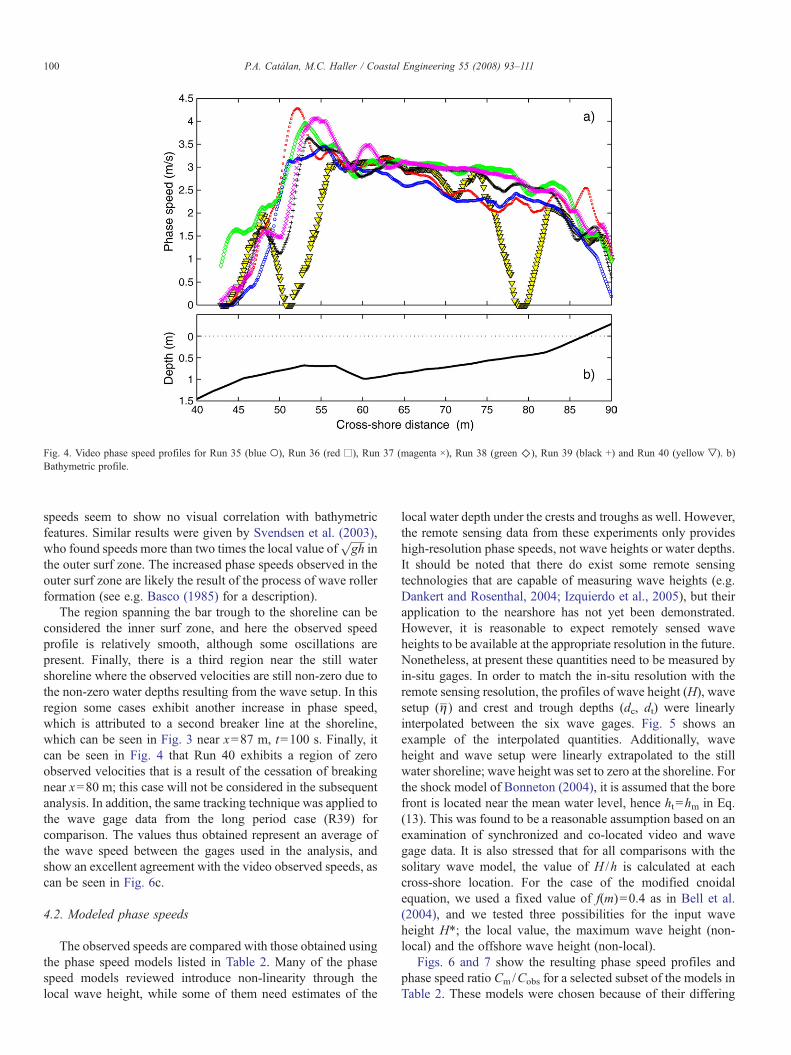
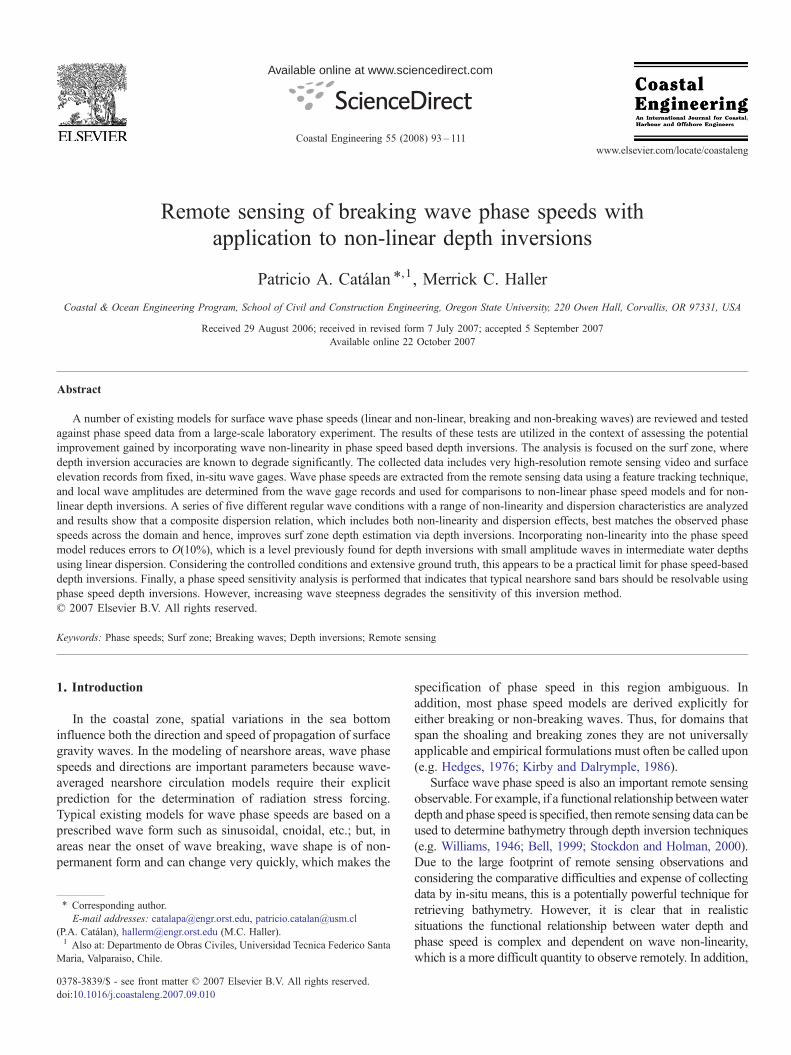
Fig. 4. Video phase speed profiles for Run 35 (blue ○), Run 36 (red □), Run 37 (magenta ×), Run 38 (green ◇), Run 39 (black +) and Run 40 (yellow ▽). b)Bathymetric profile.


speeds seem to show no visual correlation with bathymetricfeatures. Similar results were given by Svendsen et al. (2003),who found speeds more than two times the local value of

ffiffiffiffiffigh

pin

the outer surf zone. The increased phase speeds observed in theouter surf zone are likely the result of the process of wave rollerformation (see e.g. Basco (1985) for a description).

The region spanning the bar trough to the shoreline can beconsidered the inner surf zone, and here the observed speedprofile is relatively smooth, although some oscillations arepresent. Finally, there is a third region near the still watershoreline where the observed velocities are still non-zero due tothe non-zero water depths resulting from the wave setup. In thisregion some cases exhibit another increase in phase speed,which is attributed to a second breaker line at the shoreline,which can be seen in Fig. 3 near x=87 m, t=100 s. Finally, itcan be seen in Fig. 4 that Run 40 exhibits a region of zeroobserved velocities that is a result of the cessation of breakingnear x=80 m; this case will not be considered in the subsequentanalysis. In addition, the same tracking technique was applied tothe wave gage data from the long period case (R39) forcomparison. The values thus obtained represent an average ofthe wave speed between the gages used in the analysis, andshow an excellent agreement with the video observed speeds, ascan be seen in Fig. 6c.

4.2. Modeled phase speeds

The observed speeds are compared with those obtained usingthe phase speed models listed in Table 2. Many of the phasespeed models reviewed introduce non-linearity through thelocal wave height, while some of them need estimates of the

local water depth under the crests and troughs as well. However,the remote sensing data from these experiments only provideshigh-resolution phase speeds, not wave heights or water depths.It should be noted that there do exist some remote sensingtechnologies that are capable of measuring wave heights (e.g.Dankert and Rosenthal, 2004; Izquierdo et al., 2005), but theirapplication to the nearshore has not yet been demonstrated.However, it is reasonable to expect remotely sensed waveheights to be available at the appropriate resolution in the future.Nonetheless, at present these quantities need to be measured byin-situ gages. In order to match the in-situ resolution with theremote sensing resolution, the profiles of wave height (H), wavesetup (η ) and crest and trough depths (dc, dt) were linearlyinterpolated between the six wave gages. Fig. 5 shows anexample of the interpolated quantities. Additionally, waveheight and wave setup were linearly extrapolated to the stillwater shoreline; wave height was set to zero at the shoreline. Forthe shock model of Bonneton (2004), it is assumed that the borefront is located near the mean water level, hence ht =hm in Eq.(13). This was found to be a reasonable assumption based on anexamination of synchronized and co-located video and wavegage data. It is also stressed that for all comparisons with thesolitary wave model, the value of H /h is calculated at eachcross-shore location. For the case of the modified cnoidalequation, we used a fixed value of f(m)=0.4 as in Bell et al.(2004), and we tested three possibilities for the input waveheight H⁎; the local value, the maximum wave height (non-local) and the offshore wave height (non-local).

Figs. 6 and 7 show the resulting phase speed profiles andphase speed ratio Cm/Cobs for a selected subset of the models inTable 2. These models were chosen because of their differing

http://dx.doi.org/doi:10.1029/2003JC002130

Table 2Table of phase speed models used in the analysis; percent relative error of thephase speed models in the region 60.04≤x≤81.97 m, Rc mean relative errorand RRMS

c average root-mean-square error

Model Equation Rc RRMSc

Linear theory c2 ¼ gktanh ðkhÞ −7.4 10.5

Solitaryc ¼

ffiffiffiffiffiffiffiffiffiffiffiffiffiffiffiffiffiffiffiffiffiffigh 1þ H

h

r 17.9 19.2

Modified shallow c ¼ 1:3ffiffiffiffiffigh

p 24.0 25.7

Cnoidal theoryc ¼

ffiffiffiffiffiffiffiffiffiffiffiffiffiffiffiffiffiffiffiffiffiffiffiffiffiffiffiffiffiffiffiffiffiffiffiffiffiffiffiffiffiffiffiffiffiffiffiffiffigh 1þ H

mh2� m� 3E

K

h ir 7.0 9.1

Modified cnoidal c ¼ffiffiffiffiffiffiffiffiffiffiffiffiffiffiffiffiffiffiffiffiffiffiffiffiffiffiffiffiffiffiffiffiffiffiffiffiffigh 1þ f mð ÞH⁎=hð Þ

pH⁎=Hlocal 5.0 10.1H⁎=Hmax 13.3 14.7H⁎=Hoff 9.1 11.9

Bore c2b ¼ ghdcdth3

dt þ dcð Þ2

13.3 14.7

Shockc ¼ �2

ffiffiffiffiffiffiffiffighm

pþ 2

ffiffiffiffiffiffiffight

pþ

ffiffiffiffiffiffiffiffiffiffiffiffiffiffiffiffiffiffiffiffiffiffiffiffiffighcht

ht þ hc2

� � r 24.1 25.1

KD86 c2=g/k(1+ f1ϵ2D)tanh(kh+ f2ϵ) 2.8 8.0

Hedges c2 ¼ gktanh k hþ Hð Þð Þ 11.1 12.7

Booij c2 ¼ g

ktanh k hþ H=2ð Þð Þ 2.7 8.0


degrees of non-linearity (cnoidal, solitary, KD86), theirprevious application in depth inversion studies (linear) andtheir inherent basis on surf zone breaking waves (bore). Itwas found that the modified shallow water and the shockmodel overpredicted the speed significantly irrespective ofthe wave conditions. In addition, the models of Hedges(1976) and Booij (1981) exhibit a very similar trend to thatof the KD86 model. For these reasons they are not includedin the figure, whilst they remain in the overall analysis.

Fig. 5. Example of interpolated in-situ data, Run 39. Wave heightH (▽); (□) mean cres

Figs. 6 and 7 show three of the five conditions tested; themost and least dispersive (R35 and R39, respectively), and thecondition with the largest non-linearity (R37). The modelsexhibit piecewise linear phase speed profiles, which is attributedto their direct dependency on the water depth. The magnitudesof the observed speeds over the bar are bounded by the solitaryand linear models, consistent with previous findings. However,it is not immediately obvious which model provides the bestagreement. In addition, discrepancies are significant over thebar at the onset of breaking, where the direct dependency on thewater depth makes almost all models predict decelerationsfollowed by accelerations at the down slope on the shorewardside of the bar, whereas the observed speeds show exactly theopposite trend. The results for the shock model suggest it doesrelatively better in this region (not shown), but a moreconclusive analysis would require higher resolution in thenarrow region over the bar.

In the region shoreward of the bar trough (60bxb82 m), allmodels are in agreement with the observed trend of steadilydecreasing speeds consistent with a linear bathymetric profile.Overall, the linear model appears to do best at higher relativewater depths, kh, i.e. for shorter periods and larger depths.However, as waves enter shallower water the observed speedgradually approaches the KD86 model or cnoidal models, andeventually the bore model. The asymptotic behavior of thecomposite model to that of Booij (1981) means they are almostindistinguishable for most of the domain.

Agreement typically deteriorates in the region betweenx=85 m and the still water shoreline at x=86.65, where all themodels predict a sharp decay in phase speeds. All models fail topredict the observed speeds shoreward of the still watershoreline. In some cases, a large increase in the speed occursthat can be associated with a secondary breaker that is beingpicked up by the tracking algorithm.

It is of interest to compare the performance of the speedmodels in the region where all relevant parameters can be

t elevation dc; mean trough elevation dt (○) and bathymetric profile (black – – –).

Fig. 6. Comparison between modeled and observed phase speeds, a) Run 35 (H=0.6 m, T=4.0 s), b) Run 37 (H=0.5 m, T=6.0 s), c) Run 39 (H=0.4 m, T=8.0 s),d) Bathymetry. Observed (dots); linear theory (dashed thick blue); solitary (solid dotted black); cnoidal (solid magenta); KD86 (dash-dot thick red); bore (solid thinblack); In-situ speeds denoted by (•), up arrows denote the location of in-situ gages.


assumed known. For this reason, we focus our attention on theregion spanning from x=60.04 m (the bar trough) tox=81.97 m. Two criteria governed this choice. First, thephysical processes taking place over the bar crest (onset of

Fig. 7. Ratio between modeled and observed spe

breaking) are not well described by any of the models understudy. Second, model results beyond x=81.97 m rely on theextrapolated wave setup information. Both effects add anunquantifiable source of error that could mask the true

eds, Cm/Cobs. Same color coding as Fig. 6.

Fig. 8. Distribution of the absolute relative error |Rc(x)| against dispersiveness μ=kh, non-linearity δ and Ursell number, for each model tested. Run 35 (blue ○); Run36 (red □); Run 37 (magenta ×); Run 38 (green◇) and Run 39 (black +).


performance of the models in their region of applicability. Forthe analysis we use cross-shore profiles of the absolute relativeerror defined as

Rc xð Þ ¼ cmodel xð Þ � cobs xð Þcobs xð Þ ; ð18Þ

where cmodel, cobs are the modeled and observed phase speeds,respectively.

Considering the possible dependency of this error on thedispersiveness μ and non-linearity δ, each local estimate of therelative error is plotted against these parameters for the selectedmodels in Fig. 8. Here the absolute value |Rc(x)| is shown in order

Fig. 9. Ursell number as a function of dispersiveness kh for tested wave conditions w(magenta x); Run 38 (green◇) and Run 39 (black +). (For interpretation of the referenarticle.)

to simplify the analysis. It should be mentioned that for the wavesof smallest period (R 35), the limit of applicability for the cnoidalmodel (h /Lob3/8π) is broached at some locations. These pointswere removed from the data set of that particular run and noattempts were made to combine it with another model.

Dispersiveness is computed based on the local wavenumberfrom linear theory and ranges from 0.15bkhb0.81 for these tests,which corresponds to shallow to intermediate water conditions.Fig. 8 confirms that the linear model performs better wheredispersiveness dominates but has large errors in shallowwater. Therelative error also increases, as expected, with non-linearity. Botheffects are combined in the Ursell number, in which case linearwave theory performs well when non-linearity is less than or equal

ithin the limited cross-shore domain. Run 35 (blue ○); Run 36 (red □); Run 37ces to colour in this figure legend, the reader is referred to the web version of this

Fig. 10. Flowchart of the inversion algorithm. Dashed lines represent steps forlinear inversions, solid lines additional steps for non-linear inversions. For thepresent implementation, (^) denotes data with low spatial resolution.


to dispersiveness (i.e. Urb1). The opposite trend is true for theshallow, solitary and shock models, which exhibit the smallesterrors at high Ursell numbers, but large errors for the oppositeconditions (only solitary model shown). A similar trend wasobserved with the modified cnoidal model, using local values ofwave height, although the errors were smaller. Errors were larger ifnon-local values of wave height were used instead.

In general, the cnoidal model and all the composite modelsseem to have relative errors that are somewhat uniformly

Fig. 11. Estimated median depth profile using a) linear (+); b) KD86 (•) dis

distributed across all water depths with a slight increase withnon-linearity, which translates into a weak dependency on theUrsell number. Furthermore, the errors are confined in the range±20% for all values of kh and δ. Finally, the accuracy of thebore model is also dependant on dispersiveness, with the errorsincreasing with kh or for decreasing Ursell number. However,the bore model performs very well for small kh values, whichmay explain the good agreement found in previous studies.

In order to derive a single representative error value, we havetwo choices. The first is to take the cross-shore mean of theabsolute relative error profiles, and then average over all waveconditions in order to obtain a single estimate of the error for eachmodel, Rc. However, this value is subject to cancellation of valuesof the same magnitude but different sign. A root-mean-squarevalue is probably a more representative error measure. A secondrepresentative error value can be defined from the absolute relativeerror profiles determined for each model as

RcRMS ¼

ffiffiffiffiffiffiffiffiffiffiffiffiffiffiffiffiffiffiffiffiffiffiffiffiffiffiffiffiffiffiffiffiffiffiffiffiffiffiffiffiffiffiffiffiffiffiffiffiffiffiffiffiffiffiffi1N

X cmodel xð Þ � cobs xð Þð Þ2c2obs xð Þ ;

sð19Þ

where N is the total number of cross-shore locations considered.This calculation provides aRRMS

c estimate for eachmodel and eachwave condition, which are then averaged over the wave conditionsto obtain a single estimate of the error for each model RRMS

c . Thiserror measure represents the average phase speed error whenconsidering a range of incident wave conditions and observationlocations.

Columns 3 and 4 in Table 2 list each of the representative errorvalues and show that the composite (KD86 and Booij (1981)) andmodified cnoidal models have the smallest errors and aresomewhat better than the linear and bore models. The asymptoticnature of the KD86 model to that of Booij (1981) makes the two

persion model. Vertical error bars correspond to 95% confidence level.

Table 3Error estimates for individual profiles and the median profile

Case Linear KD86

D Drms R Rrms D Drms R Rrms

m m % % m m % %

35 0.05 0.10 9.41 19.26 −0.10 0.14 −13.13 20.4736 0.05 0.11 5.28 14.36 −0.12 0.16 −20.29 27.2037 0.25 0.26 41.10 44.83 0.08 0.11 14.75 19.8538 0.23 0.25 39.02 44.89 0.05 0.11 10.93 20.5539 0.15 0.18 27.15 33.30 −0.03 0.11 −1.39 15.16Median 0.17 0.18 28.20 31.65 −0.01 0.05 0.94 9.70

Cross-shore mean and rms value of the difference errors (D, Drms) and relativeerrors (R, Rrms) for each model. Analysis domain contains 60.04bxb81.97 m.


hard to distinguish for the present wave conditions and theyaccordingly yield similar relative error values. The shallow water,solitary, and shock models fair much worse, since the range ofwater depths considered well exceeds their region of validity. Thelinear model performs somewhat better than the shallow watermodels, which appears to result from the fact that Ursell numbersare not very large over a good portion of the domain for themajority of the cases studied (see Fig. 9).

In summary, the Booij (1981) and KD86 model provided thebest overall agreement, which indicates the strength of thecomposite models. The modified cnoidal model that utilized thelocal wave height measure was next best, and all of these tend tooffer good results over the range of Ursell numbers. However, theperformance of themodified cnoidalmodel is clearly dependant onthe choice of a characteristic wave height. Although other modelsmay provide better estimates locally under the appropriateconditions, the benefit of providing dispersive and non-linearbehavior in a singlemodelmakes it themost suitable for non-lineardepth inversions. The expected better performance in intermediateto deep water gives the composite models an extended range ofapplicability and an overall advantage.

4.3. Depth inversions

Up to this point, we have assessed the performance of a rangeof phase speed models in comparison to experimental data. Inthe following section, we will quantify the potential benefit ofincorporating the locally measured finite amplitude effects intothe depth inversion algorithm. Based on our previous results, wewill focus on a composite model (KD86), since the compositemodels performed the best of the non-linear models and we willcompare it to simple linear dispersion.

Local wavenumbers are estimated directly as the ratiobetween the observed phase speed and the radian frequencyσ=2πfp, where the peak frequency fp is obtained from the pixelintensity spectra. Wave amplitudes are interpolated from the in-situ data and used in conjunction with wavenumbers to invertthe appropriate dispersion relation and calculate the local meanwater depth. Inversion of the linear model is explicit

h ¼ 12k

lngk þ r2

gk � r2

� �; ð20Þ

whereas the KD86model requires an iterative procedure. Fig. 10shows the flowchart of the inversion algorithm, highlighting theadditional steps used in this study to include a local measure ofnon-linearity.

After subtracting the interpolated wave setup profiles, theresulting bathymetric profiles are compared with the known stillwater depth. Over the bar, the observed increase in speed wouldlead to a trench in the depth profiles rather than a bar (see Catalán,2005; Catalán and Haller, 2005), because as mentioned previously,none of the phase speed models can account for the rollerformation process. Hence, in order to not bias the assessment of theinversion algorithms, we again focus on the region shoreward ofthe bar trough (x=60.04 m). Individual bathymetric profiles areobtained for each wave condition, but it is also convenient to

consider the results in terms of a median profile, which is obtainedas the median of the individual estimates at each cross-shorelocation following Stockdon and Holman (2000).

Fig. 11 shows the median profiles determined from eachinversion model. Overall, the profile shape is well recovered;vertical error bars correspond to the 95% confidence level.Linear theory typically overpredicts depths, consistent withobserved velocities larger than the theoretical value, andagreement seems to deteriorate as water becomes shallowerdue to increasing non-linearity. The KD86 model for its partunderpredicts depths near the bar trough, followed by a regionof better agreement.

In order to quantify the agreement, the dimensionaldifference error D=h−htrue (in meters) and the relative errorR=D /htrue⁎100 (in %) are computed at each location for eachindividual wave condition and for the median profile. Accord-ing to these error definitions, positive values indicate depthoverprediction. Cross-shore mean (D, R) and root-mean-square(Drms, Drms) values of these statistics, calculated for the region60.04bxb81.97 m, are listed in Table 3. Again the RMS valuesare probably more representative, since mean values are subjectto cancellation.

The results can be summarized as follows:

• Analysis of the individual cases indicates that the non-linearmodel performs significantly better than the linear as relativewater depths decrease (and non-linearity increases).

• Individual profile errors using the non-linear model in thesurf zone are of the same order of magnitude as the averageerrors from previous studies using linear theory in theshoaling zone with small amplitude waves.

• If the median profile is considered, the non-linear model isfar superior with the mean relative error R reduced from 28%(32% RMS) for the linear model to 0.9% (10% RMS) withthe non-linear model.

5. Discussion

5.1. Sources of error

One of the fundamental assumptions of the standard videorectification process is that pixels image the same physical

Fig. 12. Misregistration of the pixel array. The target pixel (t) is shadowed by thefinite amplitude wave at point (v), which has a corresponding location (r) whenprojected over the pixel array.


location throughout the collection; thus, the world coordinatesof any pixel in the image are known beforehand and remaininvariant. Typically for field installations, where the distance tothe sea surface is large (O(100) m), it is assumed that the watersurface lies on a single horizontal plane (mean sea level), andvertical displacements can be neglected and do not induceartificial horizontal displacements. However, for the presentexperimental setup, grazing angles were relatively small (about14° near the shoreline along y=1.2 m) and cameras wererelatively close to the physical target (the free surface, O(20) m).Vertical displacements in the water surface will lead to videomisregistration.

One potential vertical displacement would be the splash-upof a plunging breaker, which may cause the wave front to beassociated with a pixel located shoreward of the true front. Thisisolated, local vertical displacement will translate into ahorizontal displacement along the pixel array and lead to alocal artificial excess of speed. This effect can be quantified on ageometrical basis, as shown in Fig. 12. A simple estima-tion shows that the horizontal displacements are equal toΔx=α(x−xc), where x is the cross-shore location of theobserved pixel, xc is the camera location and α=hs / (zc− z) isthe ratio between the splashing amplitude (hs) and the verticaldistance between the camera and the free surface. For breakingevents occurring near x=54 m, and with a splashing amplitudeof 30 cm, it yields translation errors of O(5)cm. If the splashingevent lasts 2 frames (t=0.2 s), the spurious velocity will beapproximately 0.25 m/s, which represents only a fraction ofmost of the observed model/data discrepancies, but may berelevant locally. In practice, a rigorous correction for this excessspeed is not possible without detailed knowledge of theinstantaneous free surface displacement and splashing height.

A second source of vertical displacement is due to finiteamplitude waves, and the associated misregistration variesinversely with grazing angle. This type of misregistration resultsin a more global cross-shore shift in the phase speed profile. The

maximum shift due to this effect is calculated to be about 70 cmand occurs in the vicinity of the still water shoreline (Catalán,2005). This is expected to have little influence on the results inthe present case.

Finally, the existence of mean currents in the surf zone is notaccounted for in the phase speed models and may contribute tomodel/data error. In this laboratory flume undertow would bethe main source of any mean current and a rough estimate of theexpected undertow velocity was obtained from the experimentsof Scott et al. (2005) for a condition similar to R36. For that casethe maximum undertow measured over the bar was ∼14% ofthe local linear phase speed, a value slightly larger than 5–8%found by Svendsen et al. (2003) in their experiments.

Considering mean currents in field applications, the effect oflongshore currents would likely be negligible based on theirquasi-orthogonality with the incident waves. In general, theeffect of undertow on phase speeds is likely exaggeratedsomewhat in 1D laboratory flumes as compared to fieldsituations where mean currents are typically more complexand two-dimensional. However, the presence of rip currentswould certainly affect the phase speed locally. Low frequencymotions can also change the local value of h over several waveperiods, hence affecting the speed of individual waves (e.g.Thornton and Guza, 1982; Madsen et al., 1997b), although theoverall effect would average out for long runs (as is the casehere).

5.2. Sensitivity of depth inversions to measurement error

It is possible to relate errors in depth retrieval withmeasurement errors in the input parameters. Using linear theoryas the basis for depth inversions, Dalrymple et al. (1998)obtained an analytical expression for the error in the depthestimate showing that the magnitude of the depth error is at leasttwice the error in the input parameter k or σ, and this factorincreases with kh. Hence, phase speed-based depth inversionmethods tend to magnify measurement errors.

A similar expression can be obtained for the KD86 model(see Appendix A for details) as given below

dhh

¼ drrF1 kh;Að Þ � dk

kF2 kh;Að Þ � dA

AF3 kh;Að Þ; ð21Þ

where δk /k, δσ /σ and δA /A correspond to relative errors (orperturbations) in wavenumber, frequency and wave amplitude.The expected errors in depth estimates using the KD86 modelexhibit similar behavior to the linear case in regards to σ and k,but also incorporate a new source of error related to themeasurement of wave amplitude, A. The functional dependencyof the functions F1, F2 and F3 on kh and A show that waveamplitude measurement errors do not get amplified as much asthose related with k or σ. This is fortunate, and our results fromthe previous section indicate that even fairly sparse measure-ments of wave amplitude can be simply interpolated and theirinclusion provides an improvement over linear depth inversionmethods. For example, if we treat Hedges model as ground


truth, then a depth estimate hcan be obtained from a measuredamplitude Ameas as

h ¼ c2

g� Ameas; ð22Þ

where c is taken as the true phase speed.Hence, the relative error is

R ¼ h� htruehtrue

¼ c2=g � Ameasð Þ � c2=g � Atrueð Þhtrue

¼ Atrue � Ameasð Þhtrue

;

ð23Þ

where Atrue is the true amplitude. Thus, when linear dispersion isused (Ameas=0) the relative error is equal to the non-linearityparameter, R=Atrue /htrue, which is in accordance with previousobservations that correlated depth inversion errors with wave non-linearity (Holland, 2001).

However, even after inclusion of non-linearity, the opera-tional accuracy of phase speed-based depth inversions isgoverned by the inherent accuracy of phase speed models(and measurements). Under the range of controlled conditionsconsidered here, and with the available high-resolution remotesensing data, the present analysis shows that phase speeds fromthe KD86 dispersion relation lie within 8% of the measuredvalues. This, in turn, places an effective limit on the vertical sizeof bathymetric features (i.e. the local depth perturbation) thatcan be resolved using phase speed depth inversion. In otherwords, the feature size that can be identified above the “noise”inherent to the model/data agreement.

Considering that under typical field conditions phase speedobservations corresponding to a range of wave heights andperiods would be available for a given beach morphologic state,

Fig. 13. Fraction ofwave conditions in the rangeT=3.0–16 s,H=0.1–3.0m capable of

then there will exist some minimum resolvable bottom featureheight (vertical amplitude), Δhmin, for those conditions. Thefunctional form of Eq. (21) can be used to estimate thisminimum height. Under the assumption that errors in phasespeed can be attributed to errors in wavenumber, it is possible toestimate the factor F2 in Eq. (21) as a function of wave period,wave height and unperturbed depth (i.e. expected depth in theabsence of the bottom feature). Once the factor F2 is calculated,the uncertainty region can be determined by

Dhmin ¼ F2⁎h⁎dkk; ð24Þ

where we choose δk /k=8%. For the case of a sand bar with localheightΔhbar above the underlying profile, ifΔhmin≤Δhbar thenthe bar would represent a perturbation larger than the underlyinguncertainty and should be detected by the method. We also notethat this approach implicitly assumes that the waves are inequilibrium with the underlying bathymetry. In fact, thisassumption underlies all phase speed models and depthinversion algorithms in general.

In order to study if bottom features typical to field beacheswould be detectable by depth inversion algorithms, minimum barheights as a function of the local unperturbed depth for a range ofincidentwave conditionswere calculated as shown in Fig. 13. Thechosen range of wave condition was T=3.0–16 s and H=0.1–3.0 m, with water depths h=0–30 m. The colored region of thefigure represents the range of observable features and indicatesthat the minimum feature size increases with water depth. Thewhite region in the left side of the figure represents surfacepiercing bars, which were removed from consideration.

In order to place these results in the context of typical barsizes and water depths as found in the field, we utilize the

detecting a bar. Dashedwhite line indicates the equilibrium bar height at each depth.

Fig. 14. Minimum identifiable perturbation size (in m) at a given depth, asfunction of wave height and wave period. a) h=5 m, b) h=10 m.).


equilibrium bar profile model of Hsu et al. (2006). Withoutgoing into detail, the model provides an analytic, barred profileshape based on given input wave conditions. The model alsorequires calibration of several empirical coefficients, which wehave done here using two barred profiles measured at Duck,NC (see Appendix B). The bar model is used here only toconstrain the bar morphologies, which are taken as independentfrom the expected wave conditions used in the phase speedanalysis. The relationship between expected bar heights anddepths is shown by the white line in Fig. 13 and turns out tobe approximately Δhbar≈h/3 based on the chosen calibrationcoefficients.

It can be seen that for this range of bar heights and depths,more than 80% of the expected wave conditions provideΔhmin≤Δhbar, and thus it is technically feasible to resolve thesesand bars using phase speed depth inversions. Of course otherfield sites may have significantly different barred profilecharacteristics and if expected bar heights are smaller theymay lie out of the observable range for a given site. In addition,

the chosen range of wave periods is probably somewhat widerthan is usually observed over a given bar location on an activebeach profile.

A slightly different approach is to identify the minimum barheight that can be observed as a function of wave conditions at aparticular (unperturbed) water depth. Fig. 14 a) and b) showcontours of minimum observable bar heights for depths ofh=5 m and 10 m, respectively. The figure indicates thatminimum perturbation size increases rapidly with relative waterdepth (i.e. as wave period decreases). This is an expected resultbased on previous understanding of the linear dispersionrelation (Dalrymple et al., 1998). However, for shallow relativedepths (longer periods) there is a clear dependency on wavesteepness (H /T) with minimum perturbation size increasingsteadily with steepness. This reflects the fact that the sensitivityof wave phase speed to the local water depth decreases as thewave non-linearity of shallow water waves increases.

6. Conclusions

The objectives of the present study were to 1) assess theaccuracy of a wide range of phase speed models when applied tonon-linear, dispersive surf zone waves, and 2) quantify thepotential improvement gained by incorporating non-linearityinto phase speed-based depth inversions. A number of phasespeed models were tested against laboratory observations, thesemodels included those explicitly derived for linear, non-linear,breaking, and non-breaking waves. The observational data usedfor comparison consisted of very high-resolution remotesensing video along with in-situ surface elevation records.The analysis was focused on the surf zone, an area whereprevious depth inversion techniques have shown low skill.Nonetheless, the observational data consisted of wavesexhibiting a range of non-linearity and dispersiveness.

The composite phase speed models (Kirby and Dalrymple,1986; Booij, 1981) incorporate non-linear effects through theadditional input of the local wave height and provided the bestagreement with remotely measured phase speeds. Other modelssuch as the bore and shock models, can at times show betterlocal agreement. However, only at limited shallow waterlocations and their requirement of multiple water depthestimates as input parameters also severely hinders their usefor depth inversions. The cnoidal wave model and a number ofmodified cnoidal models also performed relatively well.However, only when the locally measured wave heights wereused was the phase speed agreement better than with lineardispersion.

Depth inversions using both linear theory and the KD86composite model were performed in intermediate to shallowwater (0.15bkhb0.81) for each of the individual monochro-matic wave conditions. The median depth profiles were alsocalculated and these represent the net result from invertingspeeds at individual frequencies (each with their own degree ofnon-linearity) for the same bathymetry. Under field conditionsthis is analogous to synchronous measurements of phasespeeds at discrete frequencies in a random wave field. Forinversions with the composite model, utilizing results from a

Table 4Calibrated parameter space for the model of Hsu et al. (2006)

A1 A2 B1 B2 B3

2.2 1.3 3.0 2.8 −0.5


five wave conditions reduced the errors from 20% to 10%,approximately.

As compared to linear theory, using the composite modelsignificantly improved depth retrievals, with RMS errors for themedian profile reduced from 30% to 10%. Overall, the inclusionof non-linearity allowed shallow water estimates to have thesame or better accuracy as depth inversions performed inprevious studies for intermediate water depths using lineardispersion. Considering the controlled conditions and extensiveground truth in the present analysis, this appears to be a practicallimit for phase speed-based depth inversions.

Also, although only the composite model of KD86 was usedfor the depth inversions, both the KD86 and Booij (1981)models showed similar agreement to the phase speed observa-tions for the present data set. It should be noted that the Booij(1981) model is simpler to invert and may be more useful in thatsense in practical applications of the depth inversion technique.The two models may show more significant differences in highUrsell number and large relative water depth regimes (Hedges,1987; Kirby and Dalrymple, 1987). However, this could not betested with the present data set.

Finally, it was shown analytically that for the compositemodel the errors in retrieved depths are less sensitive to mea-

Fig. 15. Calibration of the model of Hsu et al. (2006) and determination of the relevantthe Duck profiles. Dashed magenta line correspond to the interpolated unperturbedreader is referred to the web version of this article.)

surement errors in the wave amplitude (as opposed towavenumber errors). A phase speed sensitivity analysis alsoindicates that typical nearshore bathymetric features (barsor depressions), should be resolvable by depth inversionsprovided the remote sensing observations are sufficientlyaccurate and the range of existing wave conditions is suffi-ciently wide. Yet, the depth inversion problem is still fairlydifficult and has a number of possible sources of error. Inaddition, it is of note that as wave steepness (H /T) increases inrelatively shallow water, the sensitivity of the phase speed tobottom perturbations must necessarily decrease. Clearly, theoverall accuracy of depth retrievals from inversion methods aredecreased from traditional surveying methods; however, thecost savings and improvements in the speed of depth acquisitionwill still make inversion techniques useful in many situations.

Acknowledgments

The authors wish to thank the staff at the O.H. HinsdaleWave Research Lab (HWRL) for the aid in conducting theexperiments, including Dan Cox, Tim Maddux, Chris Scott,and Terry Dibble. We are also in debt to Rob Holman, JohnStanley, Jason Killian, and Dan Clark of the Coastal ImagingLab for establishing the ARGUS camera station at the HWRL,which was fundamental to this work. This work was partiallysupported by the Office of Naval Research under award numberN00014-02-1-0147. P. Catalan was also supported by Depart-mento de Obras Civiles, Universidad Tecnica Federico SantaMaria, Chile.

vertical distances. Red thick line is the calibrated model; thin lines correspond toprofile. (For interpretation of the references to colour in this figure legend, the


Appendix A. Relative error for the composite model

By differentiating the KD86 model and performing somealgebra, it is possible to obtain the relative error in water depthas a function of the relative error in wavenumber, frequency andwave amplitude:

dhh

¼ drrF1 kh;Að Þ � dk

kF2 kh;Að Þ � dA

AF3 kh;Að Þ ðA:1Þ

with

F1 kh;Að Þ ¼ 2WUA1 þW B1 þ C1ð ÞU ðA:2Þ

F2 kh;Að Þ ¼ WUþ B1 þ C1 þ 2e2Df1ð ÞUþ A1 þ A2ef2ð ÞWA1Wþ B1 þ C1ð ÞU

ðA:3Þ
F3 kh;Að Þ ¼ 2e2Df1Uþ A2ef2W
A1Wþ B1 þ C1ð ÞU ðA:4Þ

where

U ¼ tanh khþ f2eð ÞW ¼ 1þ f1e2Dð Þe ¼ kAf1 ¼ tanh5 khð Þf2 ¼ kh

sinh khð Þ� �4

A1 ¼ A2 khþ 1� 4ef2khcosh khð Þsinh khð Þ

� �� A2 ¼ sech2 khþ f2eð ÞB1 ¼ 5khe2D tanh4 khð Þsech2 khð ÞC1 ¼ f1e2

2kh

sinh 4khð Þ � tanh khð Þsech2 khð Þsinh4 khð Þ � 8D

cosh khð Þsinh khð Þ

� �

D ¼ 8þ cosh 4khð Þ � 2tanh2 khð Þ8sinh4 khð Þ

This expression collapses to that derived by Dalrymple et al.(1998) for the linear dispersion relation when A=0.

Appendix B. Calibration of the equilibrium beach profile

In order to characterize the typical bar height as a function ofwater depth, the equilibrium profile of Hsu et al. (2006) wascalibrated with two barred profiles measured at the US ArmyCorp of Engineers Field Research Facility, in Duck, NC (www.frf.usace.army.mil/). In particular the profiles collected duringOctober 11, 1990 and 1994 near y=950 m were used. Theprofiles were non dimensionalized by the depth and cross-shorecoordinate at the bar crest, which enables a direct comparisonwith the model of Hsu et al. (2006), whose general expression is

H ¼ A1 1� exp�B1X� �� A2exp

�B3 1�Xð ÞsechB2 1� Xð Þþ A2exp

�B3 sechB2; ðB:1Þ

where H=h /hc, X=x/xc. The resulting parameter space isshown in Table 4 and the calibrated profile is shown in Fig. 15.

The next step is to determine the depth without the bar. It wasfound that the base term in the model of Hsu et al. (2006)yielded values that were too deep, in which case the bar heightwas about the same as the depth of the bar crest. Furthermore,this provided small values of Δhmin allowing almost fullobservance of the bars. A more conservative value was obtainedby interpolating between the bar trough and the point whereX=1.5. Then, the depth of the imaginary point under the barcrest was determined and used to characterize the unperturbeddepth. The resulting non-dimensional bar height was roughlyhalf the depth of the bar crest for this particular set.

To convert these values to dimensional units, it is necessaryto multiply it by the actual dimensional depth at the bar crest hc.An empirical relation for this quantity as a function of theincident wave period and wave height was obtained by Hsu andWang (1997) in the following form

hcLo

¼ 0:017n�1:409o W�0:265

o ; ðB:2Þ

where Lo, ξo and Wo=H / (wT) are the deep water wavelength,Iribarren number and non-dimensional fall velocity. Theaverage slope required to compute the Iribarren number wasset to β=0.035 following Stockdon and Holman (2000), and afall velocity of 1 cm/s was used. The above expression allowsestimation of the bar height at any water depth.

References

Aarninkhof, S., Ruessink, B.G., 2004. Video observations and modelpredictions of depth-induced dissipation. IEEE Transactions on Geoscienceand Remote Sensing 42 (11), 832–844 (November).

Aarninkhof, S.G.J., Ruessink, B.G., Roelvink, J.A., 2005. Nearshore subtidalbathymetry from time-exposure video images. Journal of GeophysicalResearch 110, C06011. doi:10.1029/2004JC002791.

Abbot, M.B., Minns, A.W., 1992. Computational hydraulics, 2nd Edition.Ashgate Publishing Limited.

Basco, D.R., 1985. A qualitative description of wave breaking. Journal ofWaterway, Port, Coastal, and Ocean Engineering 111 (2), 171–188.

Bell, P.S., 1999. Shallow water bathymetry derived from an analysis of X-bandmarine radar images. Coastal Engineering 37, 513–527.

Bell, P.S., Williams, J.J., Clark, S., Morris, B.D., Vila-Concejo, A., 2004. Nestedradar systems for remote coastal observations. Journal of Coastal ResearchSpecial Issue 39, 1.

Bonneton, P., 2004. Wave celerity in the surf zone. Proceedings, 29th Inter-national Conference on Coastal Engr. ASCE, pp. 392–401.

Booij, N., 1981. Gravity waves on water with non-uniform depth and current.Tech. Rep. Rep. No.81-1. Dept. Civ. Eng., Delft University of Technology.

Buhr Hansen, J., Svendsen, I.A., 1979. Regular waves in shoaling water.Experimental data. Tech. Rep. Ser. Pap. 21, Inst. Hydrodyn. Hydraul. Eng.(ISVA), Tec. Univ. Denmark, Lyngby.

Buhr Hansen, J., Svendsen, I.A., 1986. Experimental investigation of the waveand current motion over a longshore bar. Proceedings, 20th InternationalConference on Coastal Engr. ASCE, pp. 1166–1179.

Catalán, P.A., 2005. Hybrid approach to estimating bathymetry using remotesensing. M.Oc.E Thesis, Oregon State University.

Catalán, P.A., Haller, M.C., 2005. Nonlinear phase speeds and depth inversion.Coastal Dynamics '05. ASCE.

Dalrymple, R.A., Kennedy, A.B., Kirby, J.T., Chen, Q., 1998. Determiningdepth from remotely sensed images. Proceedings, 26th InternationalConference on Coastal Engr. ASCE, pp. 2395–2408.

Dankert, H., Rosenthal,W., 2004.Ocean surface determination fromX-Band radar-image sequences. Journal of Geophysical Research 109, C04016. doi:10.1029/2003JC002130.

http://www.frf.usace.army.mil/

http://www.frf.usace.army.mil/


Dingemans, M.W., 1997. Water wave propagation over uneven bottoms.Advanced Series onOcean Engineering, vol. 13.World Sci., River Edge, N.J.

Dugan, J.P., Piotrowski, C.C., Williams, J., 2001. Water depth and surfacecurrent retrievals from airborne optical measurements of surface gravitydispersion. Journal of Geophysical Research 106 (C8), 16903–16915.

Flick, R.E., Guza, R.T., Inman, D.L., 1981. Elevation and velocity measure-ments of laboratory shoaling waves. Journal of Geophysical Research 86,4149–4160.

Grilli, S.T., Skourup, J., 1998. Depth inversion for nonlinear waves shoalingover a barred-beach. Proceedings, 26th International Conference on CoastalEngr. ASCE, pp. 603–616.

Hedges, T.S., 1976. An empirical modification to linear wave theory.Proceedings of the Institution of Civil Engineers 61 (Part 2), 575–579 (Sep.).

Hedges, T.S., 1987. Discussion: an approximate model for nonlinear dispersionin monochromatic wave propagation models, by J. T. Kirby and R. A.Dalrymple. Coastal Engineering 11, 87–89.

Holland, T.K., 2001. Application of the linear dispersion relation with respect todepth inversion and remotely sensed imagery. IEEE Transactions onGeoscience and Remote Sensing 39 (11), 2060–2071.

Hsu, T.-W., Wang, H., 1997. Geometric characteristics of storm beach profiles.Journal of Coastal Research 13 (4), 1102–1110.

Hsu, T.-W., Tseng, I.-F., Lee, C.-P., 2006. A new shape function for bar-typebeach profiles. Journal of Coastal Research 22 (3), 728–736 (May).

Inman, D.L., Tait, R.J., Nordstrom, C.E., 1971. Mixing in the surf zone. Journalof Geophysical Research 76 (15), 3493–3514.

Izquierdo, P., Nieto Borge, J., Guedes Soares, C., González, R.S., Rodríguez, G.,2005. Comparison of wave spectra from nautical radar images and scalar buoydata. Journal of Waterway, Port, Coastal, and Ocean Engineering 131 (3),123–131.

Kirby, J.T., Dalrymple, R.A., 1986. An approximate model for nonlineardispersion in monochromatic wave propagation models. Coastal Engineer-ing 9, 545–561.

Kirby, J.T., Dalrymple, R.A., 1987. Discussion reply: an approximate model fornonlinear dispersion in monochromatic wave propagation models. CoastalEngineering 11, 89–92.

Komar, P., 1998. Beach Processes and Sedimentation, second edition. PrenticeHall.

Lippmann, T.C., Holman, R.A., 1991. Phase speed and angle of breaking wavesmeasured with video techniques. Coastal Sediments ' 91, vol. 1, pp. 542–556.

Madsen, P.A., Sørensen, O.R., Schäffer, H.A., 1997a. Surf zone dynamicssimulated by a Boussinesq type model. Part I. Model description and cross-shore motion of regular waves. Coastal Engineering 32, 255–287.

Madsen, P.A., Sørensen, O.R., Schäffer, H.A., 1997b. Surf zone dynamicssimulated by a Boussinesq typemodel. Part II. Surf beat and swash oscillationsfor wave groups and irregular waves. Coastal Engineering 32, 289–319.

Peregrine, D.H., 1967. Long waves on a beach. Journal of Fluid Mechanics 27,815–827.

Piotrowski, C.C., Dugan, J.P., 2002. Accuracy of bathymetry and currentretrievals from airborne optical time series of imaging of shoaling waves.IEEE Transactions on Geoscience and Remote Sensing 40 (12), 2606–2618(December).

Puleo, J.A., Farquharson, G., Frasier, S.J., Holland, K.T., 2003. Comparison ofoptical and radar measurements of surf and swash zone velocity fields.Journal of Geophysical Research 108 (C3), 3100.

Schäffer, H.A., Madsen, P.A., Deigaard, R., 1993. A Boussinesq model forwaves breaking in shallow water. Coastal Engineering 20, 185–202.

Scott, C.P., Cox, D.T., Maddux, T.B., Long, J.W., 2005. Large-scale laboratoryobservations of turbulence on a fixed barred beach. Measurement Scienceand Technology 16 (10), 1903–1912.

Stansby, P.K., Feng, T., 2005. Kinematics and depth-integrated terms in surfzone waves from laboratory measurement. Journal of Fluid Mechanics 529,279–310.

Stansell, P., MacFarlane, C., 2002. Experimental investigation of wave breakingcriteria based on wave phase speeds. Journal of Physical Oceanography 32,1269–1283.

Stive, M.J.F., 1980. Velocity and pressure field of spilling breakers. Proceedings,17th International Conference on Coastal Engr. ASCE, pp. 547–565.

Stive, M.J.F., 1984. Energy dissipation in waves breaking on gentle slopes.Coastal Engineering 8, 99–127.

Stockdon, H.F., Holman, R.A., 2000. Estimation of wave phase speed andnearshore bathymetry from video imagery. Journal of Geophysical Research105 (C9), 22015–22033.

Suhayda, J.N., Pettigrew, N.R., 1977. Observations of wave height and wavecelerity in the surf zone. Journal of Geophysical Research 82 (9), 1419–1424.

Svendsen, I.A., 1974. Cnoidal waves over a gently sloping bottom. Tech. Rep.Series Paper No. 6. Institute of Hydrodynamics and Hydraulic Engineering,Technical University of Denmark.

Svendsen, I.A., 2006. Introduction to Nearshore Hydrodynamics. AdvancedSeries on Ocean Engineering, vol. 24. World Sci., River Edge, N.J.

Svendsen, I.A., Buhr Hansen, J., 1976. Deformation up to breaking of periodicwaves on a beach. Proceedings, 15th International Conference on CoastalEngr. ASCE, pp. 477–496.

Svendsen, I.A., Veeramony, J., 2001. Wave breaking in wave groups. Journal ofWaterway, Port, Coastal, and Ocean Engineering 127 (6), 200–212.

Svendsen, I.A., Madsen, P.A., Buhr Hansen, J., 1978. Wave characteristics in thesurf zone. Proceedings, 16th International Conference on Coastal Engr.ASCE, pp. 520–539.

Svendsen, I.A., Qin, W., Ebersole, B.A., 2003. Modeling waves at the LSTF andother laboratory facilities. Coastal Engineering 50, 19–45.

Thornton, E.B., Guza, R.T., 1982. Energy saturation and phase speeds measuredon a natural beach. Journal of Geophysical Research 87 (C12), 9499–9508.

Thornton, E.B., Guza, R.T., 1983. Transformation of wave height distribution.Journal of Geophysical Research 88 (C10), 5925–5938.

Walker, J.R., 1976. Refraction of finite-height and breaking waves. Proceedings,15th International Conference on Coastal Engr. ASCE, pp. 507–524.

Williams, W.W., 1946. The determination of gradients of enemy-held beaches.Geographical Journal 107, 76–93 (July).

Remote sensing of breaking wave phase speeds with...

Documents

Transcript of Remote sensing of breaking wave phase speeds with...