Remote Sens. 2015, 7, 8489-8515; doi:10.3390/rs70708489

remote sensing ISSN 2072-4292

www.mdpi.com/journal/remotesensing

Article

On the Importance of Training Data Sample Selection in Random Forest Image Classification: A Case Study in Peatland Ecosystem Mapping

Koreen Millard * and Murray Richardson

Department of Geography and Environmental Studies, Carleton University, Ottawa, ON K1S 5B6,

Canada; E-Mail: murray_richardson@carleton.ca

* Author to whom correspondence should be addressed; E-Mail: koreen_millard@carleton.ca;

Tel.: +1-613-520-2561; Fax: +1-613-520-4301.

Academic Editors: Alisa L. Gallant and Prasad S. Thenkabail

Received: 31 March 2015 / Accepted: 23 June 2015 / Published: 6 July 2015

Abstract: Random Forest (RF) is a widely used algorithm for classification of remotely sensed

data. Through a case study in peatland classification using LiDAR derivatives, we present an

analysis of the effects of input data characteristics on RF classifications (including RF out-of-

bag error, independent classification accuracy and class proportion error). Training data

selection and specific input variables (i.e., image channels) have a large impact on the overall

accuracy of the image classification. High-dimension datasets should be reduced so that only

uncorrelated important variables are used in classifications. Despite the fact that RF is an

ensemble approach, independent error assessments should be used to evaluate RF results, and

iterative classifications are recommended to assess the stability of predicted classes. Results

are also shown to be highly sensitive to the size of the training data set. In addition to being as

large as possible, the training data sets used in RF classification should also be (a) randomly

distributed or created in a manner that allows for the class proportions of the training data to

be representative of actual class proportions in the landscape; and (b) should have minimal

spatial autocorrelation to improve classification results and to mitigate inflated estimates of

RF out-of-bag classification accuracy.

Keywords: Random Forest; classification; training data sample selection; peatland;

wetland; LiDAR

OPEN ACCESS

Remote Sens. 2015, 7 8490 1. Introduction

“Random Forest” (RF) is now a widely used algorithm for remote sensing image classification [1]. Its ability

to handle high dimensional and non-normally distributed data has made it an attractive and powerful option for

integrating different imagery sources and ancillary data sources into image classification workflows [2]. RF is

an ensemble classifier that produces many Classification and Regression (CART)-like trees, where each tree is

grown with a different bootstrapped sample of the training data, and approximately one third of the training

data are left out in the construction of each tree [3]. The input variables (i.e., image channels) are also randomly

selected for building trees. These characteristics of the algorithm allow RF to produce an accuracy assessment

called “out-of-bag” error (rfOOB error) using the withheld training data as well as measures of variable

importance based on the mean decrease in accuracy when a variable is not used in a building a tree. Breiman

considers rfOOB error to be an independent assessment of accuracy, as the sample points used in error

calculation are not used in building that tree of the “forest” for classification [3].

A number of studies have compared the results of RF classification with other classifiers (e.g., [4–6]) and

the different model parameters within RF (e.g., [7]). However, very little has been written about the

sensitivity of RF to different strategies for selecting the training data used in classification (see [8] for a recent

example). RF classifications are generally thought to be more stable than CART and commonly used

parametric techniques, such as Maximum Likelihood, due to the use of bootstrapping and a random subset

of data in building the RF model [9]. However, like other classification techniques, several aspects of the

sampling strategy used to collect training data play an important role in the resulting classification. In this

study we assess three aspects of the sampling strategy and resulting training data: sample size, spatial

autocorrelation and proportions of classes within the training sample.

Supervised image classification requires the collection of both training and validation data to produce

thematic maps of features of interest (e.g., general land cover, agricultural crops, wetland classes, etc.) [10].

Regardless of the choice of classifier, accuracy assessments are used to determine the quality of the

classification, and several factors can affect the results of an accuracy assessment, including training sample

size [11,12], the number of classes in the classification [13], the ability of the training data to adequately

characterize the classes being mapped [10], and dimensionality of the data [13]. Generally, when performing

image classification and accuracy assessments, training and validation data should be statistically

independent (e.g., not clustered) [14] and representative of the entire landscape [10,12], and there should be

abundant training data in all classes [15]. Many different training and validation sampling schemes are used

throughout the literature, but without careful scrutiny of each dataset used and the specific assessment

method, it may be difficult to compare results of classifications [11,16]. Ideally, a randomly distributed

sampling strategy should be used for obtaining training and validation data, but this method can be time

consuming and difficult to implement if ground validation is required for each

point [11,16]. However, when training and validation data are not randomly distributed (as in the use of

polygon data or homogenous areas of training data), these data violate the assumption of independence,

which has been shown to lead to optimistic bias in classification [14,17,18], where reported accuracy of the

classification is inflated [14]. Care must be taken to ensure validation points are drawn from a sample

independent of training data to avoid optimistic bias [14].

It has also been noted that statistical classifiers and machine learning algorithms may be biased where the

proportions of training or validation data classes are distributed unequally or are imbalanced relative to the

Remote Sens. 2015, 7 8491 actual land cover proportions. In these cases, the classification may favour the ‘majority’ classes within the

training data [12,19,20] (i.e., the class that represents the largest proportion in the training sample). Classes

that are over-represented in the training data may dominate the resulting classification, whereas classes that

are under-represented in the training data may also be under-represented in the classification. In such cases,

the magnitude of the bias is a function of the training data class imbalance [21]. To work with imbalanced

datasets or instances where a class represents a small portion of the training data (i.e., rare classes), over-

sampling and under-sampling are sometimes used to produce more balanced datasets [20]. For example,

Puissant et al. [22] noted classes that were rare in the landscape were also often under-represented or not

present in resulting classifications. To increase the presence of rare classes of interest, they devised a targeted

sampling strategy in which training data were selected only in areas where the rare classes were known to be

found. This targeting of the rare class resulted in a higher proportion of the class in the training data and

better representation in the resulting classification. On the other hand, such targeted sampling could lead to

overestimation of actual class proportions if not implemented judiciously. Cases of imbalanced data are likely

common in remote sensing classification, but the sensitivity of machine learning classifiers such as RF to

class proportions has not yet been thoroughly investigated.

The problems associated with imbalanced training data may be exacerbated when high dimensional

datasets are combined with small sample sizes in training datasets [20]. In such scenarios, the ability of

machine learning algorithms to learn is compromised due to the complexity involved in making

decisions to address a large number of features with limited sample points. Due to increased complexity

in high dimensional datasets, classifiers generally require a larger training sample to achieve an

acceptable level of accuracy [13]. It is common practice to reduce dimensionality of remote sensing

datasets before classification (e.g., through Principal Components Analysis) [25]. Although RF is able

to deal with high dimensional data [23,24], the results of image classification can be significantly

improved if only the most important variables are used [25]. RF produces measures of variable

importance that indicate the influence of each variable on the classification. Several authors have noted

that RF “importance” metrics are useful in determining the variables that provide the most valuable

information to the classification (e.g., [5–7,25]). To produce the accurate RF classifications, only the

most important input data should be used (i.e., only the derivatives that are most important to the

classification) [9,25], and correlated variables must first be removed from the classification.

The goal of this paper is to demonstrate the sensitivity of RF classification to different strategies for

selecting training sample points. Our case study focused on land cover mapping with LiDAR terrain and

point cloud derivatives at Alfred Bog, a large peatland complex in southeastern Ontario, Canada. This

work builds on previous research in which RF was applied to map ecosystem types in another nearby

peatland complex using a combination of LiDAR and Synthetic Aperture Radar (SAR) derivatives [25].

The specific objectives of the current study are to: (1) determine the uncorrelated important variables in

our classification and use these data in producing classifications for subsequent analysis; (2) quantify

the variability in classification results when bootstrapped classifications are run with RF; (3) quantify

the effects of training data sample size on rfOOB error and independent accuracy assessments; (4) assess

the effects of training class proportions on mapped class proportions; and (5) assess the effects of spatial

autocorrelation in training data on classification accuracy. To our knowledge, there are currently no other

systematic, quantitative assessments of how training sample size and sample selection methods impact

RF image classification results.

Remote Sens. 2015, 7 8492 Study Area and Data

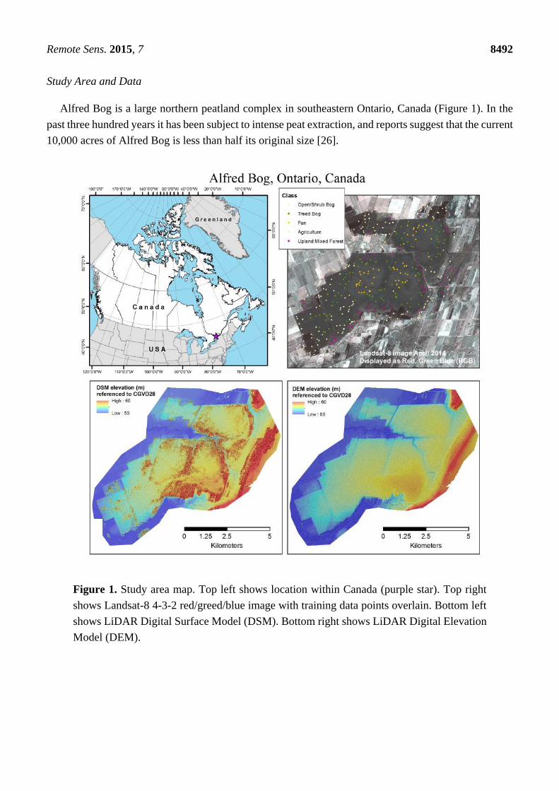
Alfred Bog is a large northern peatland complex in southeastern Ontario, Canada (Figure 1). In the

past three hundred years it has been subject to intense peat extraction, and reports suggest that the current

10,000 acres of Alfred Bog is less than half its original size [26].

Figure 1. Study area map. Top left shows location within Canada (purple star). Top right

shows Landsat-8 4-3-2 red/greed/blue image with training data points overlain. Bottom left

shows LiDAR Digital Surface Model (DSM). Bottom right shows LiDAR Digital Elevation

Model (DEM).

Remote Sens. 2015, 7 8493

Figure 2. Peatland and upland classes at Alfred Bog. Top panel indicates dominant species

found in each class with a corresponding photo. The middle panel shows boxplots of the

standard deviation of Height Vegetation classified points in each class. Boxplots in the

bottom panel indicate the Valley Depth DEM derivative in each class. Valley Depth is a

LiDAR derivative that measures the vertical distance to an inverted channel network and

indicates the local magnitude of relief. If notches in boxplots do not overlap there is strong

evidence that their medians are statistically different [34]. Photos by Marisa Ramey (2014).

Additionally, drainage ditches exist throughout the bog as a result of efforts to lower the water table

in certain areas for subsequent mining of peat. Vegetation varies throughout the bog and appears to be

affected by the presence of the drainage ditches and mined edges of the bog. The main peatland classes

Remote Sens. 2015, 7 8494 that exist at Alfred Bog are poor fen, open shrub bog and treed bog, but these classes can be quite similar

in both vegetation and topography (Figure 2). Surrounding the peatland there are mixed, coniferous and

deciduous forests with moss and low shrub understory, as well as vast agricultural areas with various

crops. In this study, we use the peatland and surrounding area as our test site for investigating the

sensitivity of RF classification to various different characteristics of training data. A LiDAR dataset is

available for the entire bog and surrounding area. A number of recent studies have demonstrated that

LiDAR derivatives provide superior classification accuracies compared with use of optical and radar

imagery (e.g., [25–29]) for both general land cover mapping and specifically in peatland mapping.

Optical imagery captures spectral reflectance from the different vegetation species visible from above.

Whereas vegetation species can be useful for differentiating many land use classes, peatland species

diversity can be very low, with a few of the same dominant species occurring in many of the classes

(Figure 2). LiDAR captures information about the form of both topography and vegetation which, in

peatlands, allows distinction between classes (Figure 2). Peatland classes often form along hydrologic

gradients, and boundaries between classes may not be clear on the ground. Also, peatland classes often

vary in vegetation structure (height, density, etc.). The ability of LiDAR to capture both topographic and

vegetation components of the landscape has been shown to improve classification accuracies in

peatlands [25,30]. In this study, we used LiDAR data for Alfred Bog to investigate the effects of training

data characteristics and selection on classification results, although our findings likely generalize to other

types of imagery. 2. Methods

2.1. LiDAR Data and Derivative Processing

LiDAR data were acquired by Leading Edge Geomatics on 30 October 2011. Data were obtained from

the vendor in Log ASCII Standard (LAS) format and were classified (ground, non-ground) using LAStools

software [31], and height above ground for each point was calculated using the LASheight command. A

Digital Elevation Model (DEM) was created from the ground classified points and a Digital Surface Model

(DSM; elevations of the top of reflective surfaces) was developed from the all-hits data using inverse

distance weighted interpolation. Several derivatives were calculated from ground and

non-ground points (using LAStools) and several were calculated based on DEM or DSM raster values

(using SAGA GIS [32]—see Table 1). Point spacing of the raw LiDAR data was approximately one point

per square meter. The calculation of derivatives requires several points per grid, therefore, these derivatives

were created at 8 m spatial resolution, as in Millard and Richardson [25]. These derivatives are hereafter

referred to as “variables.”

2.2. Training Data Collection

Selecting a random sample of training data distributed across a landscape ensures a sample that has class

proportions that are representative of the actual landscape class proportions. Training data were classified using

both field validation and high resolution image interpretation. A set of 500 randomly located points (with a

minimum point spacing of 8 m) were distributed throughout the study area. Due to the difficult nature of access

to peatlands, not all of these sites could be visited. Instead, the classes at most locations were manually

Remote Sens. 2015, 7 8495 interpreted from imagery. Expert knowledge resulting from a number of on-site field activities between 2012

and 2014 in conjunction with several ancillary image datasets were used to determine the class at each point.

The interpreter visited representative sites and recorded the location with a GPS unit, as well as the peatland

class. High- and medium-resolution optical imagery from spring, summer and fall seasons was then used along

with derived and textural parameters to interpret the class at each of the randomly located points. These ancillary

image sources were not used in subsequent classification steps.

Table 1. List of Digital Elevation Model (DEM), Digital Surface Model (DSM) and point cloud

derivatives used in classification created in SAGA [32]. Raster/point describes if the derivative

was calculated from raw LiDAR points or a raster surface [35]. Abbreviations: HAG = height

above ground; veg = vegetation; hgt = height; avg= average; and std= standard deviation.

Variable Description Raster/Point

Catchment Slope Average gradient above the flow path DEM

Channel Network Base

Level

Elevation at the channel bottom at the point where all runoff from the

watershed leaves the watershed

DEM

Diff. from Mean Difference between DEM value and mean DEM value DEM, DSM

LS Factor Slope length gradient factor [36] DEM

Max Value Maximum value of DEM within 10 × 10 grid cell window DEM, DSM

Mean Value Mean value of DEM within 10 × 10 grid cell window DEM, DSM

Min Value Minimum value of DEM within 10 × 10 grid cell window DEM, DSM

Relative Slope Pos. Distance from base of slope to grid cell DEM

Slope Slope of DEM grid cell from neighbouring grid cells [37] DEM

Standard Deviation Standard deviation of DEM surface elevations in 10 pixel window DEM, DSM

Topographic Wetness

Index

DEM derivative that models topographic control of hydrologic processes;

function of slope and upslope contributing area [38]

DEM

Valley Depth Vertical distance to inverted channel network DEM

Distance Ch. Net. Distance from grid cell to Channel Network DEM

Avg. Veg. Hgt. Average HAG of LiDAR vegetation points Point

Canopy Density Num. of points above breast height (1.32 m) divided by num. of all returns Point

Count of All-hits Total number of LiDAR points in each grid cell Point

Count Ground Points Total number of ground-classified LiDAR points in each grid cell Point

DEM Difference from

Polynomial Surface

Difference between DEM and nth order polynomial trend surface where n

= 1 to 4.

DEM

Deviation from Mean Deviation of DEM grid cell values from mean DEM value DEM, DSM

Maximum Veg. Hgt. Maximum HAG of vegetation-classified LiDAR Point

Minimum Veg. Hgt. Min. HAG of LiDAR vegetation points above breast height (1.32 m) Point

Modified Catchment Area Catchment area (calculation does not treat the flow as

a thin film as done in in conventional algorithms)

DEM

Ratio Gr. to All-hits Ratio of ground-classified LiDAR points to all points per grid cell Point

SAGA Topographic

Wetness Index

Topographic wetness calculated using the Modified

Catchment Area

DEM

Std. Veg. Hgt. Standard deviation of HAG of vegetation-classified LiDAR Point

Terrain Ruggedness Sum of change in each grid cell based on neighboring grid cells DEM

Trend Surface nth Order 1st-order polynomial of DEM surface DEM

Vegetation Cover The number of first returns above the breast height (1.32 m) divided by the

number of all first returns and output as a percentage

Point

Remote Sens. 2015, 7 8496

Five land cover classes were chosen based on descriptions of wetland types in the Canadian Wetland

Inventory [33] and using knowledge of the field site acquired through numerous field surveys. The map

classes included open shrub bog, treed bog, and fen, as well as two upland classes (mixed forest and

agricultural areas).

2.3. RF Classification

RF classification was run in R Statistics [34] open-source statistical software. The randomForest [39] and

raster [40] packages were used to produce all classifications. One thousand trees were grown for each

classification. The number of trees required to maintain a certain level of accuracy has been assessed by

several authors, and the minimum number of trees for optimal classification appears to be somewhat variable

(fewer than 100 [7] to 300 trees [4]). Therefore, using 1000 may not be necessary, but does not harm the

model [3], and variable importance is said to stabilize with a larger number of trees [39]. Other variables that

can be set in the randomForest package, including mtry (the number of variables tried at each split in node),

were left at their default values. The basic script used for RF classification is provided in Appendix A. RF

classification produces measures of “out-of-bag error” (rfOOB error).

Independent validation was also conducted for comparison to rfOOB error. For each classification,

100 data points were withheld from the training data used for classification. Once the classification was

completed, the manually interpreted class for each reserved point was compared with the RF predicted

class. From this, the number of incorrectly classified points divided by the total number of points

provided the percentage classification error.

2.4. Variable Reduction

Previous research has shown that although RF can handle high dimensional data, classification

accuracy remains relatively unchanged when only the most important predictor variables are used [25].

When running the classification several times with all variables (referred to as “All Variables”)

classification (number of variables = 28), we noted that the most important variables varied among

classifications, even when the same training data were used. Therefore, we ran the RF classification 100

times and recorded importance rankings of the top five most important variables for each iteration

(Table 2). It was evident that among these important variables, several of the variables were highly

correlated. Spearman’s rank-order correlation was used to determine pair-wise correlations. Starting

with the most frequently classified important variable and moving to successively less important ones,

highly correlated (r > 0.9) variables were systematically removed leaving a set of only the most important

and uncorrelated training data variables (Table 3). This allowed us to run two additional classifications,

one with all of the variables that were found to be very important (referred to as “Important Variables”

classification (number of variables = 15)) and one with only the uncorrelated important variables

(referred to as “Uncorrelated Important” classification (number of variables = 9)). We note that if the

training set size is reduced, the set of variables in these subsets may be different, as they are chosen

based on the data available (e.g., n = 100). The set of variables used also affects the classification quality,

and, thus, error may be higher when there is more uncertainty about the important variables. Therefore,

the results obtained in this study when reducing the size of the training set are most likely optimistic.

The alternative is to re-select the important variables for every different subset of sample points. This

Remote Sens. 2015, 7 8497 would not allow the classifications to be fairly compared, as they would be created using different

variables. Therefore, we have chosen to use the same variables in all subsets.

The McNemar test [10,41] was used to determine whether statistically significant differences existed

between pairs of classifications (e.g., All Variables vs. Important Variables, Important Variables vs. Important

Uncorrelated Variables). This test requires the number of grid cells classified correctly by both classifications,

the number of grid cells classified incorrectly by both classifications, the number of grid cells classified

correctly by the first classification but not the second and vice versa [41,42], which are derived from the

confusion matrices produced through both rfOOB error and independent error assessments.

Each classification was run 25 times and classification probability maps were created that indicate

the number of times a grid cell was labeled as the most frequently classified class, showing the

uncertainty of each cell in the classification. For example, in a two-class classification, if a cell is labeled

as the most frequently occurring class in 51 of 100 classifications, then the classification is somewhat

unstable for that cell. Conversely, a cell that is labelled as the winning class 99 of 100 times indicates a

more stable classification and hence higher confidence.

Table 2. The number of times each variable was determined to be among the top five most

important variables for each of 100 classification runs.

Removed

due to

Correlation

Number of

Times “Most

Important”

Number of

Times

“2nd Most

Important”

Number of

Times

“3rd Most

Important”

Number of

Times

“4th Most

Important”

Number of

Times

“5th Most

Important”

Valley Depth 52 22 10 4 6

Std. Veg. Height 20 37 20 7 7

Max. Veg. Height 13 17 21 23 8

Trend Surface 1 10 0 0 1 0

Veg Cover 4 10 18 16 17

Veg Density 1 3 3 19 17

Trend Surface 2 0 10 20 16 18

DEM Diff Trend 1 0 1 1 0 1

Avg. Veg. Height 0 0 1 44 0

Mean DEM 0 0 3 1 6

Canopy Height Model 0 0 1 0 1

Max Dem 0 0 1 2 3

DEM 0 0 1 1 5

Min DEM 0 0 0 8

DEM Diff Trend 3 0 0 0 1 2

2.5. Effect of Training Data Sample Size on RF Image Classification

Classifications were run with varying sizes of the training dataset. For each iteration, 100 random points

were set aside for validation from the original 500 points. From the remaining 400 points for training, we

created different random sample subsets for training with 90%, 80%, 70%, 60%, 50%, 40%, and 30% of

the data, and ran classifications based on these subsets 25 times each. For each classification, rfOOB error

was calculated and an independent validation was performed using the withheld points.

Remote Sens. 2015, 7 8498

Table 3. Most important variables selected by randomForest, and pairwise correlation.

Valley

Depth

Std. Veg

Height

Max. Veg

Height

Trend

Surface 1

Veg

Cover

Veg

Density

Trend

Surface 2

DEM Diff

Trend 1

Avg. Veg

Height

Mean

DEM

Canopy

Height

Model

Max

Dem DEM

Min

DEM

DEM Diff

Trend 3

Valley

Depth −0.19 −0.14 0.25 −0.06 −0.08 0.21 −0.52 −0.14 −0.06 −0.05 −0.06 −0.07 −0.06 −0.56

Std. Veg

Height −0.19 0.87 0.30 0.80 0.82 0.40 0.24 0.87 0.47 0.80 0.47 0.47 0.47 0.15

Max. Veg

Height −0.14 0.87 0.26 0.94 0.96 0.38 0.26 0.99 0.46 0.88 0.46 0.46 0.47 0.15

Trend

Surface 1 0.25 0.30 0.26 0.25 0.25 0.90 −0.41 0.26 0.69 0.25 0.70 0.69 0.69 −0.37

Veg Cover −0.06 0.80 0.94 0.25 0.99 0.37 0.19 0.93 0.42 0.90 0.42 0.42 0.43 0.09

Veg Density −0.08 0.82 0.96 0.25 0.99 0.37 0.22 0.95 0.44 0.90 0.43 0.44 0.44 0.11

Trend

Surface 2 0.21 0.40 0.38 0.89 0.37 0.37 −0.14 0.38 0.83 0.37 0.84 0.83 0.83 −0.32

DEM Diff

Trend 1 −0.52 0.24 0.26 -0.41 0.19 0.22 −0.14 0.26 0.30 0.18 0.30 0.30 0.31 0.79

Avg. Veg

Height −0.14 0.87 0.99 0.26 0.93 0.95 0.38 0.26 0.46 0.87 0.46 0.46 0.47 0.16

Mean DEM −0.06 0.47 0.46 0.69 0.42 0.44 0.83 0.30 0.46 0.40 0.999 0.999 0.999 0.20

Canopy

Height

Model

−0.05 0.80 0.88 0.25 0.90 0.90 0.37 0.18 0.87 0.40 0.40 0.40 0.41 0.07

Max Dem −0.06 0.47 0.46 0.70 0.42 0.43 0.84 0.30 0.46 0.999 0.40 0.998 0.996 0.20

DEM −0.07 0.47 0.46 0.69 0.42 0.44 0.83 0.30 0.46 0.999 0.40 0.998 0.998 0.21

Min DEM −0.06 0.47 0.47 0.69 0.43 0.44 0.83 0.31 0.47 0.999 0.41 0.996 0.998 0.21

DEM Diff

Trend 3 −0.56 0.15 0.15 −0.37 0.09 0.11 -0.32 0.79 0.16 0.20 0.07 0.20 0.21 0.21

Remote Sens. 2015, 7 8499

2.6. Effect of Training Data Class Proportions on RF Image Classification

From the full set of 500 points, the random validation set (n = 100) and the random training dataset

(n = 400) were separated. Subsets of the training data were then created to examine the effect of the

proportion of training data in different classes. We ensured that the same total number of training data

were used in each set of data (i.e., we varied the number of points within each class, keeping the total

number of points the same). Different subsets of training data were created by forcing the proportion of

the training data per class to range from 10% to 90%, with the remaining training data split evenly across

the other classes (Figure 3). For each class and forced proportion, we ran RF 25 times with a random

sub-sample of the training data and reserved data for independent validation. The forced class

proportions were maintained within the 25 random subsets of training data.

Figure 3. Flow chart describing the methods used to create each sample of data with ‘forced

proportions’ in each class.

Remote Sens. 2015, 7 8500

Figure 4. Flow chart describing the methods used to create each sample of data with

simulated spatial autocorrelation. (a) Five hundred randomly located sample points were

created. (b) One hundred of these points were randomly set aside as validation points.

(c) Buffers were created at specified distances around the training and validation points.

(d) Grid cells were used to represent equally spaced points. To ensure groups of spatially

autocorrelated sample points were used in extracting training data and not a random sample

of individual points that fell within the buffers, the number of grid cells that would fall within

each buffer for each buffer size (8 m, 16 m, and 32 m), based on an 8 m resolution raster,

were determined. The total number of training sample points required (400) was divided by

the number of grid cells per buffer to determine the total number of buffers to select, and the

cells associated with those buffers were used in training. (e) Each selected buffer was

converted to grid cells and all of the cells within each selected buffer were used as training

data points. The validation sample points were selected randomly from the training data

points in the original dataset that had not been used in the creation of the buffers.

2.7. Effect of Spatial Autocorrelation of Training Data on RF Image Classification

To investigate the effect of spatial autocorrelation on the resulting classifications, the training data

were subset to create different levels of spatial autocorrelation (Figure 4). In creating these datasets, the

same total number of points was maintained in each class. Buffers were created at three different sizes

(8 m, 16 m, and 32 m) around training data sample points. Each buffer was converted to raster at 8 m

resolution in order to create a set of equally spaced points throughout the defined zone. To ensure groups

Remote Sens. 2015, 7 8501

of spatially autocorrelated sample points were used in extracting training data and not a random sample

of individual points that fell within the buffers, we first determined the number of grid cells that would

fall within each buffer for each buffer size (8 m, 16 m, and 32 m) based on an 8 m resolution raster. The

total number of training sample points required (400) was divided by the number of grid cells per buffer

to determine the total number of buffers to select (e.g., if there were 12 grid cells for each buffer, we

required 33 buffers to create 400 sample points) and the cells associated with those buffers were used in

training. This resulted in three datasets with the same total number of grid cells but with varying degrees

of spatial autocorrelation of the data varied (increased with buffer size). In cases where buffers

overlapped (and classes in overlapping buffers were the same), the overlapping buffers did not result in

duplicate points as the rasterization process would result in a single set of regularly spaced cells for these

buffers. Only three cases occurred at the 32 m buffer level where overlapping buffers were of different

classes (e.g., bog and fen). In these cases, the buffer with the larger area in an overlapping cell would be

the resulting class. Since these instances were so few, the removal of a few points did not greatly affect

the number of cells in these classes. In cases where the training data point did not fall on the intersection

of grid cells depending on its exact location, the number of cells represented by each buffer may be

slightly different than in the case where the point falls on the cell corner. Therefore, the sample sizes

may vary slightly from expected (e.g., for a 16 m buffer, the actual number of cells beneath buffers

ranged from 10 to 14, with the average being 12.2 and the expected number being 12).

To measure spatial autocorrelation, Moran’s I (local) [43] was computed for each of the training

datasets. Finally, a subset of the original training data points were selected that were not used to create

the spatially-autocorrelated training data to use for independent validation. This ensured that the

validation data were distributed throughout the entire image and not spatially autocorrelated with the

training data. A Wilcoxon Rank Sum test [44] was used to confirm that the mean values of each of the

predictor variables in the training datasets were the same as the original dataset. The largest buffer size

where the means were equal was 32 m. Beyond this buffer size (e.g., 64 m buffers) the means of the

sample points were different than the original non-spatially autocorrelated sample.

3. Results

3.1 Variable Reduction

McNemar’s tests highlighted differences among the classification results where different subsets of

variables were used. Out-of-bag error rates were the same (α = 0.95) for All Variables versus Important

Variables (p = 0.5). The independent assessment error for these two classifications was statistically

significantly different (p < 0.01). The classification accuracy with Important Variables was the same as

with Uncorrelated Important Variables using rfOOB error (p = 0.8), but comparison with the independent

assessment points yielded statistically different accuracy results (p < 0.1). In comparing rfOOB error and

independent assessment error for all classification pairs, the McNemar test found the error matrices of the

rfOOB error and independent assessment error to be different (p < 0.0001).

Remote Sens. 2015, 7 8502

Figure 5. Comparison of classifications based on All Variables (a), Important Variables (b),

and Uncorrelated Important (c). Maps on the left demonstrate the most frequently predicted

class in 25 iterations and maps on the right indicate the number of times the most commonly

predicted class was classified based on 25 iterations. In the All Variables classification, many

cells demonstrate a low probability of being classified as the most commonly predicted class.

In the other two classifications, most of the cells demonstrate moderate to high probability

of being classified as the most commonly predicted class. Although similar, the Important

Variables and Uncorrelated Important Variables classifications are statistically significantly

different according to the McNemar’s test.

Remote Sens. 2015, 7 8503

Figure 6. Probability analysis indicating the percentage of times each grid cell was classified as a particular class in 25 iterations of the

classification with Uncorrelated Important Variables. A random selection of 100 of the 500 sample points was reserved each time for

independent validation. (a) Most frequently classified. (b–f) Percentage of times each pixel was classified as a specific class.

Remote Sens. 2015, 7 8504

Although the rfOOB error was similar for the three classifications, the classification with All Variables

had much larger average and maximum errors with the independent assessment than did the classification

for the Important Variables and Uncorrelated Important Variables (Table 4). Examining the resulting

classifications showed that when using many variables (e.g., in this case all variables), there was noise in the

resulting classification (Figure 5). Additionally, there is greater variability in the number of times grid cells

were classified the same in iterative classifications when using all variables (Figures 5 and 6). In all

classifications, we see that there is some confusion near the edges of wetland classes, and the extent of

wetland classes is somewhat variable between the 25 iterations, as can be seen in the classification probability

maps (Figure 5) and class probability maps (Figure 6). When a grid cell is classified as a particular class

100% of the time, the classification is stable for that cell. This is the case for most areas that were classified

as agriculture, as there is little overlap between the values of the derivatives in the agricultural class and any

of the peatland classes (Figure 2). However, thousands of grid cells classified as one of the peatland classes

show variability in the number of times they were classified as a specific class, and this is especially prevalent

near the edges of class boundaries (e.g., Treed Bog and Fen; Figure 6). Boxplots of the mean classification

error (Uncorrelated Important Variables) for each peatland class were computed based on 25 iterations of

classifications. These indicate that the agricultural class resulted in the lowest error, with low variability

across the 25 iterations (Figure 7). The fen class also resulted in relatively low error, but with higher

variability in error across the iterations. Open shrub bog and treed bog resulted in higher mean error, but the

variability in error of treed bog was significantly smaller than in open shrub bog, potentially indicating

instability in the classification of open shrub bog.

Figure 7. Boxplots showing mean classification error for each class based on 25 iterations

of classification.

Remote Sens. 2015, 7 8505

Table 4. Mean, Minimum (min), Maximum (max) and standard deviation (Std. Dev.) of rfOOB

error and independent assessment error (Indep.) for 25 iterations of each of three classifications.

All Variables Important Variables Uncorrelated Important Variables

rfOOB Indep. rfOOB Indep. rfOOB Indep.

Mean 23.4 38.5 24.4 26.8 27.3 26.7

Min 19.8 36.0 24.0 20.0 25.4 18.0

Max 27.0 45.0 29.0 28.0 31.3 29.0

Std. Dev. 1.7 2.2 1.3 2.3 1.4 3.1

Figure 8. Mean of rfOOB and independently assessed error for 25 iterative classifications

varying the sample size with All Variables (a), Important Variables (b), and Uncorrelated

Important Variables (c).

3.2. Size of Training Data Set and Classification Accuracy

By varying the sample size and running classifications iteratively 25 times, it was evident that when using

high dimensional data, the RF out-of-bag error was underestimated (inflated accuracy) compared to the

independently assessed error (rfOOB error = 23% and independent assessment error = 38.5% for

n = 400; Figure 8). The difference between rfOOB error and independently assessed error decreased slightly

as sample size decreased, indicating that even with a larger training dataset the rfOOB error was not a good

indicator of error for high dimensional datasets. However, as sample size increased, error in general

decreased; therefore, increasing sample size significantly should lead to improved classification accuracy.

When dimensionality was reduced so that only the most important variables were considered (Important

Variables Classification), rfOOB error and independent assessment error were much more similar (rfOOB

error = 24% and independent assessment error = 28% for n = 400; Figure 8), and with small sample sizes (n

< 200) rfOOB error actually over-estimated error relative to the independent accuracy assessment (validation

n = 100; Figure 8). For the Uncorrelated Important Variables Classification rfOOB error was very slightly

Remote Sens. 2015, 7 8506

over-estimated with larger sample sizes, but within a few percent of the independently assessed error and

was not statistically significantly different. Independent assessment error was generally lowest with the

Uncorrelated Important Variables Classification, except for when small sample sizes were used, although

the classification accuracy was very similar to results for the Important Variables Classification. Independent

assessment error in the Uncorrelated Important Variables Classification was lowest where 300 sample points

were used and increased slightly with larger sample sizes. As sample size decreased the standard deviation

of error across the 25 iterations increased.

3.3. Training Data Class Proportions and Classification Accuracy

As the training data were selected using a randomly distributed spatial sample, the proportions of data in

each land cover class were representative of the actual proportions within the landscape. The proportions of

classes in the training data sample ranged between 13–34% (Table 5). When subsets of the training data were

created to proportionally reduce the amount of data used for a given class, the resulting classifications

demonstrated that there can be a large difference between the actual proportion of a specific class found in

the landscape and the proportion predicted by RF (Figures 9 and 10). The difference between the actual and

predicted proportions can be thought of as the “error” in the predicted proportions and will be referred to as

“proportion-error”. As the proportion of the class of interest in the training dataset increased, the resulting

proportion of that class in the predicted image also increased (Figure 10). Overall, rfOOB and independent

assessment error for the classifications also increased as the proportion of training samples for the class of

interest increased (Figure 10). Once the proportion of the class of interest was increased to near its actual

proportion in the landscape, that class always became the class with the lowest proportion-error. As its

proportion increased beyond its actual proportion in the landscape, rfOOB error tended towards zero and the

proportion-error for that class increased (not shown here).

Table 5. Actual proportions of each class in training data.

Class Percentage of Points in Original Training Data Sample Size

Agriculture 34 170

Treed Bog 24 120

Open shrub bog 15 75

Upland Mixed Forest 14 70

Fen 13 65

3.4. Spatial Autocorrelation of Training Data and Classification Accuracy

Comparing datasets with different levels of spatial autocorrelation confirmed that optimal training

data collection should be created with a random selection of points with low spatial autocorrelation. The

level of spatial autocorrelation within each of our training datasets is listed in Table 6, as well as the

mean error of each classification. As spatial autocorrelation of training data increased, rfOOB error

decreased while independent assessment error increased. This is an especially important consideration

when the analyst uses polygon-based training areas to define training pixels, as the grid cells within these

areas will typically exhibit high spatial autocorrelation.

Remote Sens. 2015, 7 8507

Figure 9. Classifications where training data were proportionally increased for a given class.

In all cases, as the proportion of training data for the class increased, the difference between

the actual and predicted proportions increased.

Remote Sens. 2015, 7 8508

Figure 10. Difference between the actual and predicted proportions of each class in the

classification when the proportion of training data used for each class was manipulated.

Table 6. rfOOB and independent assessment error based on classifications with varying levels of spatial autocorrelation.

8 m Buffer 16 m Buffer 32 m Buffer

n 400 400 400

Moran’s I (local) 0.11 0.45 0.70

rfOOB error Indep. Error rfOOB error Indep. Error rfOOB error Indep. Error

Mean 27.3 26.7 1.8 30.4 0 40.7

Min 25.4 18 1.5 29.7 0 40.1

Max 31.3 29 2.1 31.1 0 41.9

Std. Dev. 1.4 3.1 0.2 0.3 0 0.4

Remote Sens. 2015, 7 8509

4. Discussion

The process of training data creation for remote sensing image classification requires the analyst to

make methodological choices that present tradeoffs in data quality (i.e., class representativeness) and

quantity. For example, training data points where field validation has been completed result in high

certainty in the training data set. However, these points are often difficult to obtain and therefore there

may be a tendency for researchers to use fewer training data sample points. In peatlands and other remote

environments, time and access constraints may require researchers to obtain training sample points from

imagery without actually conducting field validation (i.e., through image interpretation, as has been done

here). In some cases the certainty of the class of a training data sample point may be low but a greater

number of training data sample points may be collected quickly and easily through this method, allowing

for a larger training data sample size.

Overall, the results of this study demonstrate that RF image classification is highly sensitive to

training data characteristics, including sample size, class proportions and spatial autocorrelation. Using

a larger training sample size produced lower rfOOB and independent assessment error rates. As with

other classifiers, larger training sample sizes are recommended to improve classification accuracy and

stability with RF. Running iterative classifications using the same training and input data was found to

produce different classification results, and the RF variable importance measures and rankings varied

with iterative classifications. Therefore, the list of important variables from a single RF classification

should not be considered stable. Although RF itself is an ensemble approach to classification and

regression modelling, we recommend replication of RF classifications to improve classification

diagnostics and performance.

Previous studies have demonstrated that RF performs well on high dimensional data, however, our

results also show that variable reduction should be performed to obtain the optimum classification. When

high dimensional datasets were used, classification results were noisy, despite creating an RF model

with 1000 trees. Independent assessment error analysis also indicated that with high dimensional data

RF may significantly underestimate error. Moreover, we demonstrated that removing highly correlated

variables from the most important variables led to an increase in accuracy and, although slight, this

difference was statistically significant (McNemar’s test, p < 0.1). Removing variables of lesser

importance also improved the stability in classification, and the difference between rfOOB and

independent assessment error was significantly reduced. Dimensionality can be considered relative to

training sample size, and therefore if more training sample points had been available our classification

results might have improved. Collection of training data sample points is time consuming and a limiting

factor in the quality of resulting classifications.

One broad assumption when collecting training data and performing image classification is that

classes are mutually exclusive and have hard, well-defined boundaries [16], something that is rare in

natural environments such as forests or wetlands. Peatlands, for example, are subject to local variation

and gradients in ground water and hydrologic conditions that could greatly affect their plant species

composition [45]. Hydrologic gradients may result in gradients in nutrients and water chemistry, leading

to gradients in plant species composition near the boundaries of classes. Even with detailed

LiDAR-derived information about topography and vegetation, peatland classes are continuous in nature

and this is problematic when classifiers result in hard boundaries. Areas of gradation and edges of classes

Remote Sens. 2015, 7 8510

are most likely to be misclassified, and mapping the probability of classification can identify areas that

should be assessed more carefully or that represent unique ecotonal characteristics. In this case study,

when training data are randomly sampled and classifications iteratively run, the agricultural class was

stable through most of the iterations, but there was variability in the classifications near the edges of

wetland classes. Although this is related to the continuous nature of peatland classes, mapping these

boundaries accurately is often the main goal of a classification or mapping exercise, as the processes

occurring in and external influences affecting these classes may be different.

A widely used method of collecting training data is for an image interpreter to visually assess an

image and draw polygons around areas where a certain class is known to exist. This method produces

highly clustered training sample points with inherently high spatial autocorrelation. Training data are

produced when the grid cell value of each input derivative is extracted from the location of the training

data point. The extracted grid cell values become the predictor data used in the classification and the

interpreted class at that location becomes the training response. Since rfOOB error is calculated using a

subset of the training data, the individual points in each validation subset will be highly similar to the

training points when a training dataset with high spatial autocorrelation is provided to the classifier.

Training data points are highly clustered, and therefore their predictor values are similar to the other

points around them; when used in classification they will produce good results in areas where the training

data predictors are similar to the predictor data used in classification. This means that areas near the

spatially autocorrelated training data will result in high classification accuracy, and therefore drawing

validation data points from a spatially autocorrelated sample will appear to be well classified while areas

outside these locations are not being tested. When rfOOB error assessments are performed, RF draws its

validation data from the training data sample provided. Therefore, if training data are spatially

autocorrelated, rfOOB error will be overly optimistic. Three levels of spatial autocorrelation were

simulated and we found the classification results to be very different and rfOOB-based accuracies to be

very inflated when training data exhibited spatial autocorrelation. This has serious implications for the

interpretation of the results from RF classification. If researchers do not report the level of spatial

autocorrelation in their training data, it will be difficult to know if the classification has been subject to

sample bias, as simulated in this study.

As the training data used here were randomly distributed, it is assumed that the proportions of training

data within the sample are similar to the proportions of classes found throughout the landscape. However,

when training data are selected using visually-interpreted homogenous areas, it is unlikely that the training

data will reflect the true class proportions in the landscape. When interpreters are selecting training data

through the traditional method they may be biased in their selection of training data to the classes that they

are most certain in identifying or feel are most important. In the case of wetland mapping, interpreters may

be biased towards selecting a larger proportion of training data sample points in wetland classes and, in this

case, RF would over-predict the proportion of wetland cover in the final classification.

When training datasets were created where class proportions were forced to artificial levels,

classification results reflected the forced proportions. When a class was under-represented in the training

data, it was often under-represented in the output classification. There was one exception: Upland Mixed

Forest was over-represented in the output classification when its proportions were simulated to be 10%

of the training sample (actual proportion was estimated to be 14%), however this was a very small over-

estimation (e.g. less than 5%) and this is likely due to the random selection process of RF, although it

Remote Sens. 2015, 7 8511

should also be noted that this class had the highest classification error in general. Once a class was

represented by more than its actual proportion, RF predicted a greater proportion of that class in the

classification results. These results indicate the importance of carefully selecting training data sample

points without bias and so that landscape proportions are maintained. Often sampling strategies are

designed so that an equal number of training data sample points are located within each class. However,

when classes were simulated here with an equal number of training data in each class (20% of sample

points in each of the five classes) those classes that were over-represented in the training sample were

also over-represented in the predicted classification. Those that were under-represented in the training

data were under-represented in the predicted classification. This again demonstrates the importance of

using a randomly distributed or proportionally-representative sampling strategy. If under-sampling

occurs within a class, the full statistical characteristics of that class may not be provided as data to the

classifier, and therefore pixels of that class may be misclassified and their extent may be under-estimated.

This implies that for rare classes, if over-sampling is undertaken to obtain a prediction for that class in

the resulting classification, it may actually be falsely over-estimated. It is likely that collecting more

training data samples would provide more training data to the classifier enabling a better representation

of the statistical characteristics and variability of these proportionately-smaller classes.

5. Conclusions

Due to its ability to handle high dimensional datasets from various sources, to produce measures error

and variable importance, and its ability to outperform many other commonly used approaches, the RF

classification technique is now a widely used method for automated classification of remotely sensed

imagery. However, we have demonstrated that the results of RF classification can be inconsistent

depending on the input variables and strategy for selecting the training data used in classification. Based

on the results of this case study in mapping peatland and upland classes, we recommend that the

following methods be used in selecting input data for RF classification:

1. High-dimension datasets should be reduced. Using only important, uncorrelated variables will

result in less inflation in rfOOB accuracy and more stable classifications.

2. Despite the fact that RF itself is an ensemble approach, iterative classifications are required to

assess the stability of predicted class extents. Probability maps of iterative classifications can be

used to examine the gradient boundaries of classes or may provide insight into the quality of

training data in these areas.

3. As many training and validation sample points should be collected as possible and independent

error assessments should be used to evaluate the quality of the classification.

4. An unbiased sampling strategy that ensures representative class proportions should be used to

minimize proportion-error in the final classification.

5. Spatial autocorrelation should be minimized within the training and validation data sample points

though an appropriate sampling strategy. When spatial autocorrelation of training data samples is

low, rfOOB error will be similar to independent error assessments.

Overall, this study demonstrates the importance of careful design of training and validation datasets

in order to avoid classification bias and inflated accuracy assessments when using RF. Moreover,

Remote Sens. 2015, 7 8512

researchers are encouraged to assess and report training and validation data characteristics and their

possible implications for image classification outputs and mapping products. Researchers should avoid

relying on accuracy assessments produced by the RF classifier that are not based on independent

validation data.

Acknowledgments

The authors would like to thank three anonymous reviewers and the guest editor who provided

comments and feedback that have helped to improve the manuscript. We would also like to thank Marisa

Ramey for her contribution to image interpretation, collecting field data and photos, and Melissa Dick,

Cameron Samson, Alex Foster, Lindsay Armstrong, Julia Riddick, Keegan Smith, Melanie Langois and

Doug Stiff for field data collection. South Nation Conservation Authority is acknowledged for providing

funding for equipment and the purchase of the LiDAR data. This research was supported by the National

Sciences and Engineering Council (NSERC).

Author Contributions

Millard and Richardson jointly conceived of and designed the experiments. Millard wrote the R

scripts, performed the experiments and analyzed the results. Millard wrote the first drafts of the paper

and Richardson contributed edits and advice on content.

Conflicts of Interest

The authors declare no conflicts of interest.

References 1. Ozesmi, S.; Bauer, M. Satellite remote sensing of wetlands. Wet. Ecol. Manage. 2002, 10, 381–402. 2. Kloiber, S.; Macloud, R.; Smith, A.; Knight, J.; Huberty, B. A semi-automated, multi-source data

fusion update of a wetland inventory for east-central Minnesota. Wetlands 2015, 35, 335–348.

3. Breiman, L. Random Forests. Mach. Learn. 2001, 45, 5–32.

4. Akar, O.; Gungor, O. Integrating multiple texture methods and NDVI to the RF classification

algorithm to detect tea and hazelnut plantation areas in northeast Turkey. Int. J. Remote Sens. 2012,

36, 442–464.

5. Adam, E.; Mutang, O.; Rugege, D.; Ismail, R. Discriminating the papyrus vegetation (Cyperus

papyrus L.) and its co-existent species using RF and hyperspectral data resampled to HYMAP.

Int. J. Remote Sens. 2012, 33, 552–569.

6. Sonobe, R.; Tani, H.; Wang, X.; Kobayashi, N.; Simamura, H. Parameter tuning in the support

vector machine and RF and their performance in cross- and same year crop classification using

TerraSAR-X. Int. J. Remote Sens. 2014, 25, 7898–7909.

7. Lawrence, R.; Wood, S.; Sheley, R. Mapping invasive plants using hyperspectral imagery and

Breiman Cutler classifications (randomForest). Remote Sens. Environ. 2005, 100, 356–362.

Remote Sens. 2015, 7 8513

8. Corcoran, J.; Knight, J.; Gallant, A. Influence of multi-source and multi-temporal remotely sensed

and ancillary data on the accuracy of random forest classification of wetlands in Northern

Minnesota. Remote Sens. 2013, 5, 3212–3238.

9. Strobl, C.; Malley, J.; Tutz, G. An introduction to recursive partitioning: Rationale, application and

characteristics of classification and regression trees, bagging and RF. Psychol. Method. 2009, 14,

323–348.

10. Foody, G. Thematic Map comparison: Evaluating the statistical significance of differences in

classification accuracy. Photogramm. Eng. Remote Sens. 2004, 70, 627–633.

11. Congalton, R. A review of assessing the accuracy of classifications of remotely sensed data. Remote

Sens. Environ. 1991, 37, 35–46.

12. Foody, G.; Mathur, A. Toward intelligent training of supervised image classifications: Directing

training data acquisition for SVM classification. Remote Sens. Environ. 2004, 93, 107–117.

13. Pal, M.; Mather, P. An assessment of the effectiveness of decision tree methods for land cover

classification. Remote Sens. Environ. 2003, 86, 554–565.

14. Hammond, T.; Verbyla, D. Optimistic bias in classification accuracy assessment. Int. J. Remote

Sens. 1996, 7, 1261–1266.

15. Räsänen, A.; Kuitunen, M.; Tomppo, E.; Lensu, A. Coupling high resolution satellite imagery with

ALS-based canopy height model and digital elevation model in object-based boreal forest habitat

type classification. ISPRS J. Photogramm. Remote Sens. 2014, 94, 169–182.

16. Foody, G. Status of land cover classification accuracy assessment. Remote Sens. Environ. 2002, 80,

185–201.

17. Friedl, M.; Woodcock, C.; Gopal, S.; Muchoney, D.; Strahler, A.; Barker-Scaaf, C. A note on

procedures used for accuracy assessment in land cover maps derived from AVHRR data.

Int. J. Remote Sens. 2000, 21, 1073–1077.

18. Zhen, Z.; Quakenbush, L.; Stehman, S.; Zhang, L. Impact of training and validation sample

selection on classification accuracy assessment when using reference polygons in object-based

classification. Int. J. Remote Sens. 2013, 34, 6914–6930.

19. He, H.; Garcia, E. Learning from imbalanced data. IEEE Trans. Knowl. Data Eng. 2009, 21,

1263–1284.

20. Breidenbach, J.; Naesset, E.; Lien, V.; Gobakken, T.; Solberg, S. Prediction of species specific

forest inventory attributes using nonparametric semi-individual tree crown approach based on fused

airborne laser scanning and multi-spectral data. Remote Sens. Environ. 2010, 114, 911–924.

21. Stumpf, A.; Lachiche, N.; Malet, J-P.; Kerle, N.; Puissant, A. Active Learning in the Spatial Domain

for Remote Sensing Image Classification. IEEE Trans. Knowl. Data Eng. 2014, 52, 2492–2507.

22. Puissant, A.; Rougier, S.; Strumpf, A. Object-oriented mapping of urban trees using Remote

Sensing classifiers. Int. J. Appl. Earth Obs. Geoinf. 2014, 26, 235–245.

23. Cutler, D.; Edwards, T.; Beard, K.; Cutler, A.; Jess, K.; Gisbon, J.; Lawler, J. RFs for classification

in ecology. Ecology 2007, 88, 2783–2792.

24. Gislason, P.; Benediktsson, J.; Sveinsson, J. RFs for land cover classification. Pattern Recognit.

Lett. 2006, 27, 294–300.

25. Millard, K.; Richardson, M. Wetland mapping with LiDAR derivatives, SAR polarimetric

decompositions, and LiDAR-SAR fusion using a RF classifier. Can. J. Remote Sens. 2013, 39, 290–307.

Remote Sens. 2015, 7 8514

26. Bird and Hale Ltd. Alfred Bog Peatland Inventory and Evaluation; Consultant Report; Bird and Hale

Ltd.:Toronto, ON, Canada, 1984. Available online: http://www.geologyontario.mndmf.gov.on.ca/

mndmfiles/afri/data/imaging/31G07NW0001/31G07NW0001.pdf (accessed on 2 June 2015).

27. Chasmer, L.; Hopkinson, C.; Veness, T.; Quinton, Q.; Baltzer, J. A decision-tree classification for

low-lying complex land cover types within the zone of discontinuous permafrost. Remote Sens.

Environ. 2014, 143, 73–84.

28. Maxwell, A.; Warner, T.; Strager, M.; Conley, J.; Sharp, J. Assessing machine learning algorithms

and image and lidar derived variables for GEOBIA classification of mining and mine reclamation.

Int. J. Remote Sens. 2015, 36, 954–978.

29. Corcoran, J.; Knight, J.; Pelletier, K.; Rampi, L.; Wang, Y. The effects of point or polygon based training

data on RandomForest classification accuracy of wetlands. Remote Sens. 2015, 7, 4002–4025.

30. Andrew, M.; Wulder, M.; Nelson, T. Potential contributions of remote sensing to ecosystem service

assessments. Progr. Phys. Geogr. 2014, 38, 328–353.

31. LAStools-Efficient Tools for LiDAR Processing; Version 140430; 2014. Available online:

http://lastools.org (accessed on 2 June 2015).

32. SAGA GIS System for Automated Geoscientific Analyses; 2014. Available online:

www.sagagis.org (accessed on 2 June 2015).

33. National Wetlands Working Group. Canadian Wetland Classification System; Warner, B.G.,

Rubec, C.D.A., Eds.; Wetlands Research Center, University of Waterloo: Waterloo, ON, Canada,

1997.

34. R Core Team. R: A Language and Environment for Statistical Computing; R Foundation for

Statistical Computing, Vienna, Austria, 2014.

35. Wilson, J.P.; Gallant, J.C. Terrain Analysis: Principles and Applications; John Wiley & Sons: New

York, NY, USA, 2000; p. 479.

36. Desmut P.; Govers, G. A GIS Procedure for automatically calculating the USLE LS factor on

topographically complex landscape units. J. Soil Water Conser. 1996, 51, 427–433.

37. Olaya, V. Basic land-surface parameters. In Geomorphometry: Concepts, Software, Applications

Developments in Soil Science; Developments in Soil Science Volume 33; Hengle, T., Reuter, H.,

Eds.; Elsevier: Dordrecht, The Netherlands, 2008; pp. 141–169.

38. Kopecky, M.; Cizkova, C., Using topographic wetness index in vegetation ecology: Does the

algorithm matter? Appl. Veg. Sci. 2010, 13, 450–459.

39. Liaw, A.; Wiener, M. Classification and regression by randomForest. R News 2002, 2, 18–22.

40. Hijmans, R. raster: Geographic Data Analysis and Modeling; R package version 2.3; 2014.

41. Dietterich, T. Approximate statistical tests for comparing supervised classification learning

algorithms. Neural Computat. 1998, 10, 1895–1923.

42. Duro, D.; Franklin, S.; Dube, M. A comparison of pixel-based and object-based image analysis with

selected machine learning algorithms for the classification of agricultural landscapes using

SPOT-5 HRG imagery. Remote Sens. Environ. 2012, 118, 259–272.

43. Anselin, L. Local indicators of spatial association—LISA. Geogr. Anal. 1995, 27, 93–115.

44. Wilcoxon, F. Some rapid approximate statistical procedures. Ann. New York Acad. Sci. 1950, 52,

804–814.

Remote Sens. 2015, 7 8515

45. Bridgham, S.; Pastor, J.; Janssens, J.; Chapin, C.; Malterer, T. Multiple limiting gradients in

peatlands: A call for a new paradigm. Wetlands 1996, 16, 45–65. © 2015 by the authors; licensee MDPI, Basel, Switzerland. This article is an open access article

distributed under the terms and conditions of the Creative Commons Attribution license

(http://creativecommons.org/licenses/by/4.0/).