Remote Identification andQuantification of IndustrialSmokestack Effluents via ImagingFourier-Transform SpectroscopyK E V I N C . G R O S S , *K E N N E T H C . B R A D L E Y , A N DG L E N P . P E R R A MDepartment of Engineering Physics, Air Force Institute ofTechnology, 2950 Hobson Way, Wright-Patterson AFB,Ohio 45433-7765, United States

Received May 28, 2010. Revised manuscript receivedSeptember 28, 2010. Accepted October 21, 2010.

Industrial smokestack plume emissions were remotelymeasured with a midwave infrared (1800-3000 cm-1) imagingFourier-transform spectrometer operating at moderatespatial (128 ! 64 with 19.4 ! 19.4 cm2 per pixel) and highspectral (0.25 cm-1) resolution over a 20 min period. Strongemissions from CO2, H2O, SO2, NO, HCl, and CO were observed.A single-layer plume radiative transfer model was used toestimate temperature T and effluent column densities qi foreach pixel’s spectrum immediately above the smokestack exit.Across the stack, temperature was uniform with T ) 396.3( 1.3 K (mean ( stdev), and each qi varied in accordance withthe plume path length defined by its cylindrical geometry.Estimated CO2 and SO2 volume fractions of 8.6 ( 0.4% and380 ( 23 ppmv, respectively, compared favorably with in situmeasurements of 9.40 ( 0.03% and 383 ( 2 ppmv. Total in situNOx concentration (NO + NO2) was reported at 120 ( 1ppmv. While NO2 was not spectrally detected, NO was remotelyobserved with a concentration of 104 ( 7 ppmv. Concentrationestimates for the unmonitored species CO, HCl, and H2Owere 14.4 ( 0.3 ppmv, 88 ( 1 ppmv, and 4.7 ( 0.1%, respectively.

IntroductionOptical remote sensing of chemical plumes is a mature fieldof research and fills an important role in the monitoring ofgaseous and particulate emissions from chemical and energyproduction facilities (1, 2). For example, while in situcontinuous emissions monitoring sensors are used to ensurefacility compliance with environmental regulations, remotesensing methods can provide an independent verification ofemissions compliance. Optical methods also enable sensingover a wide area and are useful in studying plume dispersionand atmospheric transport. Active sensing techniques, whichtypically rely on a laser tunable over a narrow spectral bandto interrogate the source, have been developed and suc-cessfully applied to smokestack and flare monitoring (3-5).Active techniques are well suited to detecting and quantifyingspecific molecules or atoms at concentrations as low as onepart per billion volume but are typically limited to inter-rogation of one or two species due to the limited bandwidthof the laser source. Additionally, active systems tend to have

a larger experimental footprint and are often more costlyand time-consuming to deploy when compared to currentpassive sensing techniques. The most common passivetechnique for smokestack monitoring is Fourier-transformspectrometry (FTS) (1, 6-13). The measurements rely onthermal emissions from effluent gases and particulatematerial, and the signal strength is a function of both columndensity and thermal contrast with the background. SinceFTS can measure spectral emissions across a wide spectralbandpass at arbitrary (in principle) spectral resolution withexcellent efficiency, it is well suited to the identification andquantification problem for multiple effluents. Given that acomplete set of calibrated plume measurements can be madein a few hours (including setup and tear-down) by a singleoperator, modern FTS systems are an attractive option forindependent emissions compliance measurements.

Imaging Fourier-transform spectrometers (IFTS) haverecently become commercially available and could substan-tially improve the accuracy of species quantification andenhance understanding of plume phenomenology. At typicalstand-off distances (0.1-1 km), the narrow single pixel field-of-view minimizes the effects of averaging over spatial regionswhich exhibit sizable changes in temperature and speciesconcentrations. This means that simpler models can be usedto interpret the spectrum. Furthermore, while temperatureand concentration gradients may exist in the plume, spectralimagery of the axi-symmetric plume at the stack exit providethe constraining data needed to successfully use “onion-peeling” tomographic deconvolution methods to determinethe plume structure (14, 15). Since radiative transfer modelsare necessary to accurately extract effluent column densities(9), the ability to simultaneously capture both the plumeand background radiation in a single spectral image isadvantageous. Spectrally resolved imagery also makes de-coupling effluent concentration from plume path lengthstraightforward, and this is useful when a priori knowledgeof the stack inside diameter is unavailable. Spectral imageryalso affords smart clustering of spectrally similar (thoughnot necessarily adjacent) pixels to increase signal-to-noise(SNR) for trace species identification without complicatingthe spectral analysis that can accompany simple spatialaveraging. Also noteworthy is the DC image that is part ofIFTS data due to use of a focal plane array (FPA). While itreduces the dynamic range available for measuring themodulated signal that encodes the spectral information, itis beneficial in the analysis and processing of interferogramscollected from turbulent sources (16, 17). Moreover, the abilityto visualize and track turbulent eddies in the DC imagerymakes possible the estimation of plume flow rates, whichwhen coupled with concentrations could yield total effluentmass flow rates.

In this work, we present the first quantitative midwave(3-5.5 µm) IFTS measurements of a plume from a coal-firedelectrical plant. After identifying the species from theirspectral signatures, a simple radiative transfer model isdeveloped which enables accurate interpretation of themeasured spectra immediately above the smokestack exitusing temperature and effluent column densities. Spectralimagery is used to remove plume path length effects, andspectral estimates of effluent concentrations are favorablycompared with in situ measurements.

Experimental SectionInstrument Description. The Telops, Inc. (Quebec, Canada)Hyper-Cam is an imaging Fourier-transform spectrometerwhich couples a traditional Michelson interferometer to an

* Corresponding author phone: (937)255-3636 x4558; e-mail:Kevin.Gross@afit.edu.

Environ. Sci. Technol. 2010, 44, 9390–9397

9390 9 ENVIRONMENTAL SCIENCE & TECHNOLOGY / VOL. 44, NO. 24, 2010 10.1021/es101823z ! 2010 American Chemical SocietyPublished on Web 11/11/2010

infrared camera. A sequence of modulated intensity imagescorresponding to optical path differences are collected on aFPA forming an interferogram cube (i.e., an interferogramat each pixel). Fourier transformation of each pixel’s inter-ferogram produces a raw ultraspectral image. Two internalwide-area blackbody sources maintained at distinct tem-peratures are used to calibrate the raw spectra at each pixelusing established procedures (18). The maximum optical pathdifference (MOPD) defines the (unapodized) spectral resolu-tion via !" ) 0.6/MOPD. In this work, spectral units will beexpressed in wavenumbers with units cm-1 and defined by" ) "/c where " is frequency (Hz) and c is the speed of light(cm · s-1) in vacuum. The IFTS uses a 320 ! 256 pixel Stirling-cooled InSb FPA which is responsive on 1800-6667 cm-1.The instrument’s minimum focal distance is 3 m. Theintegration time of the FPA can be increased from a minimumof 1 µs to adapt to the scene brightness. Each pixel has aninstantaneous field-of-view of 0.326 mrad, and a subset ofpixels can be read out to improve acquisition rate at theexpense of FOV size. The rate at which ultraspectral imagescan be acquired depends on spectral resolution, FPAintegration time, and the number of pixels in the image. TheHyper-Cam’s mean single-pixel noise equivalent spectralradiance (19) for a 1s observation of a 50 °C blackbody at 32cm-1 resolution using a FPA integration time of 5 µs is 4.1nW/(cm2 · sr · cm-1). Additional instrument (20, 21) details can befound in the references.

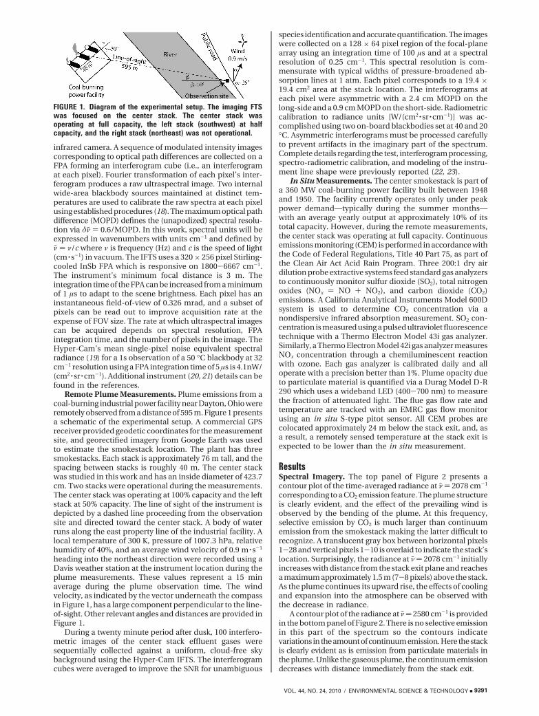
Remote Plume Measurements. Plume emissions from acoal-burning industrial power facility near Dayton, Ohio wereremotely observed from a distance of 595 m. Figure 1 presentsa schematic of the experimental setup. A commercial GPSreceiver provided geodetic coordinates for the measurementsite, and georectified imagery from Google Earth was usedto estimate the smokestack location. The plant has threesmokestacks. Each stack is approximately 76 m tall, and thespacing between stacks is roughly 40 m. The center stackwas studied in this work and has an inside diameter of 423.7cm. Two stacks were operational during the measurements.The center stack was operating at 100% capacity and the leftstack at 50% capacity. The line of sight of the instrument isdepicted by a dashed line proceeding from the observationsite and directed toward the center stack. A body of waterruns along the east property line of the industrial facility. Alocal temperature of 300 K, pressure of 1007.3 hPa, relativehumidity of 40%, and an average wind velocity of 0.9 m · s-1

heading into the northeast direction were recorded using aDavis weather station at the instrument location during theplume measurements. These values represent a 15 minaverage during the plume observation time. The windvelocity, as indicated by the vector underneath the compassin Figure 1, has a large component perpendicular to the line-of-sight. Other relevant angles and distances are provided inFigure 1.

During a twenty minute period after dusk, 100 interfero-metric images of the center stack effluent gases weresequentially collected against a uniform, cloud-free skybackground using the Hyper-Cam IFTS. The interferogramcubes were averaged to improve the SNR for unambiguous

species identification and accurate quantification. The imageswere collected on a 128 ! 64 pixel region of the focal-planearray using an integration time of 100 µs and at a spectralresolution of 0.25 cm-1. This spectral resolution is com-mensurate with typical widths of pressure-broadened ab-sorption lines at 1 atm. Each pixel corresponds to a 19.4 !19.4 cm2 area at the stack location. The interferograms ateach pixel were asymmetric with a 2.4 cm MOPD on thelong-side and a 0.9 cm MOPD on the short-side. Radiometriccalibration to radiance units [W/(cm2 · sr · cm-1)] was ac-complished using two on-board blackbodies set at 40 and 20°C. Asymmetric interferograms must be processed carefullyto prevent artifacts in the imaginary part of the spectrum.Complete details regarding the test, interferogram processing,spectro-radiometric calibration, and modeling of the instru-ment line shape were previously reported (22, 23).

In Situ Measurements. The center smokestack is part ofa 360 MW coal-burning power facility built between 1948and 1950. The facility currently operates only under peakpower demand—typically during the summer months—with an average yearly output at approximately 10% of itstotal capacity. However, during the remote measurements,the center stack was operating at full capacity. Continuousemissions monitoring (CEM) is performed in accordance withthe Code of Federal Regulations, Title 40 Part 75, as part ofthe Clean Air Act Acid Rain Program. Three 200:1 dry airdilution probe extractive systems feed standard gas analyzersto continuously monitor sulfur dioxide (SO2), total nitrogenoxides (NOx ) NO + NO2), and carbon dioxide (CO2)emissions. A California Analytical Instruments Model 600Dsystem is used to determine CO2 concentration via anondispersive infrared absorption measurement. SO2 con-centration is measured using a pulsed ultraviolet fluorescencetechnique with a Thermo Electron Model 43i gas analyzer.Similarly, a Thermo Electron Model 42i gas analyzer measuresNOx concentration through a chemiluminescent reactionwith ozone. Each gas analyzer is calibrated daily and alloperate with a precision better than 1%. Plume opacity dueto particulate material is quantified via a Durag Model D-R290 which uses a wideband LED (400-700 nm) to measurethe fraction of attenuated light. The flue gas flow rate andtemperature are tracked with an EMRC gas flow monitorusing an in situ S-type pitot sensor. All CEM probes arecolocated approximately 24 m below the stack exit, and, asa result, a remotely sensed temperature at the stack exit isexpected to be lower than the in situ measurement.

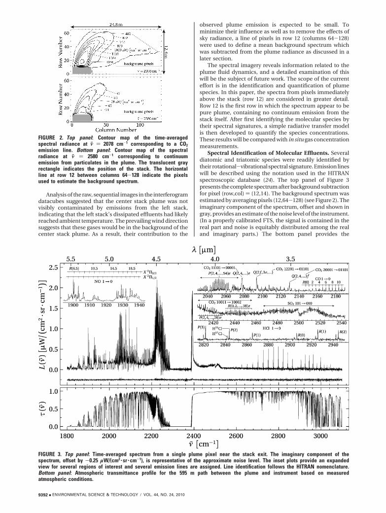
ResultsSpectral Imagery. The top panel of Figure 2 presents acontour plot of the time-averaged radiance at " ) 2078 cm-1

corresponding to a CO2 emission feature. The plume structureis clearly evident, and the effect of the prevailing wind isobserved by the bending of the plume. At this frequency,selective emission by CO2 is much larger than continuumemission from the smokestack making the latter difficult torecognize. A translucent gray box between horizontal pixels1-28 and vertical pixels 1-10 is overlaid to indicate the stack’slocation. Surprisingly, the radiance at " ) 2078 cm-1 initiallyincreases with distance from the stack exit plane and reachesa maximum approximately 1.5 m (7-8 pixels) above the stack.As the plume continues its upward rise, the effects of coolingand expansion into the atmosphere can be observed withthe decrease in radiance.

A contour plot of the radiance at ")2580 cm-1 is providedin the bottom panel of Figure 2. There is no selective emissionin this part of the spectrum so the contours indicatevariations in the amount of continuum emission. Here the stackis clearly evident as is emission from particulate materials inthe plume. Unlike the gaseous plume, the continuum emissiondecreases with distance immediately from the stack exit.

FIGURE 1. Diagram of the experimental setup. The imaging FTSwas focused on the center stack. The center stack wasoperating at full capacity, the left stack (southwest) at halfcapacity, and the right stack (northeast) was not operational.

VOL. 44, NO. 24, 2010 / ENVIRONMENTAL SCIENCE & TECHNOLOGY 9 9391

Analysis of the raw, sequential images in the interferogramdatacubes suggested that the center stack plume was notvisibly contaminated by emissions from the left stack,indicating that the left stack’s dissipated effluents had likelyreached ambient temperature. The prevailing wind directionsuggests that these gases would be in the background of thecenter stack plume. As a result, their contribution to the

observed plume emission is expected to be small. Tominimize their influence as well as to remove the effects ofsky radiance, a line of pixels in row 12 (columns 64-128)were used to define a mean background spectrum whichwas subtracted from the plume radiance as discussed in alater section.

The spectral imagery reveals information related to theplume fluid dynamics, and a detailed examination of thiswill be the subject of future work. The scope of the currenteffort is in the identification and quantification of plumespecies. In this paper, the spectra from pixels immediatelyabove the stack (row 12) are considered in greater detail.Row 12 is the first row in which the spectrum appear to bepure plume, containing no continuum emission from thestack itself. After first identifying the molecular species bytheir spectral signatures, a simple radiative transfer modelis then developed to quantify the species concentrations.These results will be compared with in situ gas concentrationmeasurements.

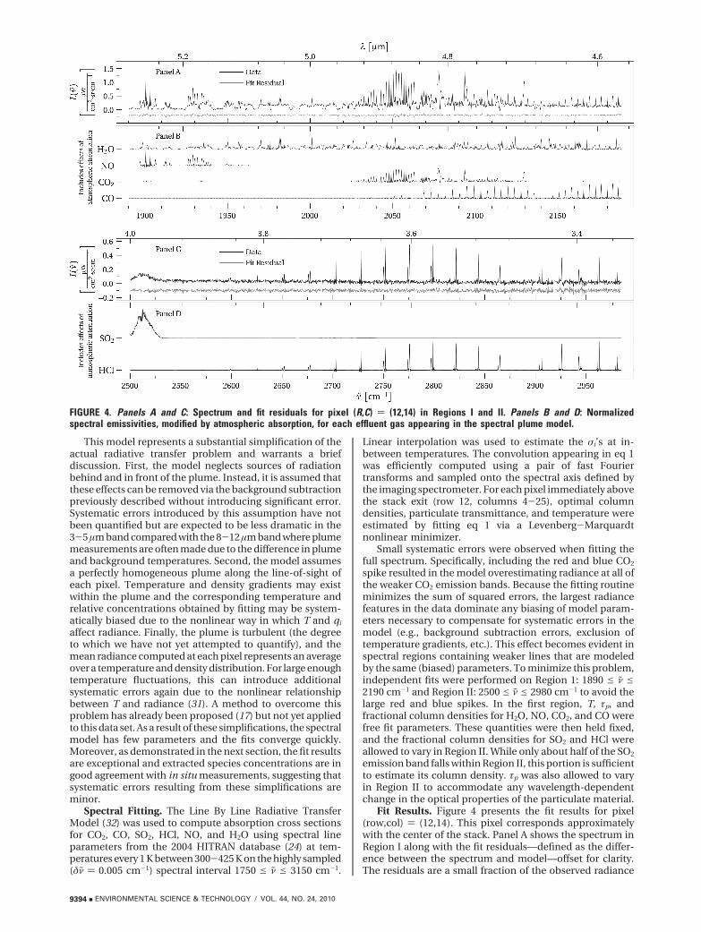
Spectral Identification of Molecular Effluents. Severaldiatomic and triatomic species were readily identified bytheir rotational-vibrational spectral signature. Emission lineswill be described using the notation used in the HITRANspectroscopic database (24). The top panel of Figure 3presents the complete spectrum after background subtractionfor pixel (row,col) ) (12,14). The background spectrum wasestimated by averaging pixels (12,64-128) (see Figure 2). Theimaginary component of the spectrum, offset and shown ingray, provides an estimate of the noise level of the instrument.(In a properly calibrated FTS, the signal is contained in thereal part and noise is equitably distributed among the realand imaginary parts.) The bottom panel provides the

FIGURE 2. Top panel: Contour map of the time-averagedspectral radiance at ! ) 2078 cm-1 corresponding to a CO2emission line. Bottom panel: Contour map of the spectralradiance at ! ) 2580 cm-1 corresponding to continuumemission from particulates in the plume. The translucent grayrectangle indicates the position of the stack. The horizontalline at row 12 between columns 64-128 indicate the pixelsused to estimate the background spectrum.

FIGURE 3. Top panel: Time-averaged spectrum from a single plume pixel near the stack exit. The imaginary component of thespectrum, offset by -0.25 µW/(cm2 · sr ·cm-1), is representative of the approximate noise level. The inset plots provide an expandedview for several regions of interest and several emission lines are assigned. Line identification follows the HITRAN nomenclature.Bottom panel: Atmospheric transmittance profile for the 595 m path between the plume and instrument based on measuredatmospheric conditions.

9392 9 ENVIRONMENTAL SCIENCE & TECHNOLOGY / VOL. 44, NO. 24, 2010

atmospheric transmittance profile along the 595 m pathestimated from local meteorological measurements. Nearlyall the absorption features are due to atmospheric H2O (1800e " e 2160 cm-1 and 2600 e " e 3080 cm-1) and CO2 (2280e " e 2390 cm-1). The observed spectrum is qualitativelysimilar in both features and absolute radiance to previouslypublished spectra of coal-fired smokestack emissions (1, 25).

Perhaps the most easily recognized spectral features arethe P- and R-branch emission lines between 2650 cm-1 and3000 cm-1 arising from the fundamental HCl vibrationaltransition. Lines P(1) – P(10) beginning at " ) 2865 cm-1 anddecreasing with " at nearly regularly spaced intervals areobserved. Similarly, lines R(0) – R(5) beginning at " ) 2906cm-1 and increasing with " are recognized despite several ofthe lines being strongly attenuated by atmospheric H2O andbeing near the edge of good instrument response. At !" )0.25 cm-1 resolution, it is possible to resolve the H35Cl (taller)and H37Cl (shorter) lines. For each rotational-vibrationaltransition, the line heights are in proportion to the 76:24isotopic abundance. The bottom inset plot of the top panelof Figure 3 shows the first few lines from the HCl P- andR-branches. The SNR of the P(4) line at 2798.9 cm-1 isapproximately 40.

The most prominent spectral features arise from therotational structure associated with transitions betweenvarious CO2 vibrational levels. For example, the large, narrowemission feature at 2395 cm-1 arises from rotational transi-tions involving the asymmetric stretching mode. While mostemission lines associated with this mode are subsequentlyabsorbed by atmospheric CO2 along the line-of-sight, thehigh plume temperature increases the population of higher-energy rotational levels leading to emission outside thisopaque region. Similarly, emission is observed on the low-wavenumber edge of this opaque region for the same reason,and various other rotation-vibration transitions thermallyaccessible at the elevated plume temperature contribute thereas well. This pattern of strong CO2 emission on each side ofthe same CO2 absorption feature is found in many combus-tion plumes, and the large emission features are often referredto as the red (longer wavelength) and blue (shorter wave-length) spike (26). CO2 is responsible for several otheremission features and the top-right and middle-right insetplots in Figure 3 identify them using spectroscopic notationadopted by the HITRAN database (24) and described in ref27.

CO and SO2 are also easily recognized in the plumespectrum, and their respective emission bands are indicatedin the top-right and middle-right inset panels of Figure 3,respectively. Spectral identification of NO was more difficultwith most of its emission lines being strongly or completelyattenuated by atmospheric water; the few that were partiallytransmitted are labeled in the leftmost inset plot of Figure3. Finally, a large number of emission lines from H2O aredistributed through the spectrum. While they are notidentified in Figure 3, their presence will be evident whena spectral model is compared to the data in the followingsection.

Spectral Modeling for Quantification and Interpretation.Theory. A simple model describing the apparent plumeradiance is developed to quantitatively interpret a pixel’sspectrum in terms of the temperature and relative concen-trations of the plume constituents. It is assumed that theplume is in local thermodynamic equilibrium (LTE) and thatscattering, background radiation, and self-emission from theatmosphere can be ignored. These assumptions (to bediscussed later) simplify the radiative transfer problem suchthat the apparent radiance L(") at a pixel can be expressedas

where # denotes the atmospheric transmittance profilebetween the instrument and plume, $ represents the plume’sspectral emissivity, and B is Planck’s distribution for black-body radiation at temperature T. The convolution with theinstrument line shape function, ILS, accounts for theresolution of the instrument. For a Fourier-transform spec-trometer, ILS is defined by the length and symmetry of theinterferogram as well as any apodization functions used toattenuate spectral ringing that occurs as a consequence ofthe finite interferogram length (28). No apodization wasapplied, and the interferogram symmetrization process (22)yielded the canonical FTS line shape function given by ILS(")) 2asinc(2%a") where a ) 2.4 cm is the instrument MOPD.

The spectral emissivity can be expressed as

Here, qi represents the product of the ith species’ volumefraction &i and the path length through the plume l, and wedenote the quantity qi ) &il the “fractional column density”.N is the total gas density [molec · cm-3] and is related to theplume pressure P (assumed equal to the atmosphericpressure) and temperature T via the ideal gas law, i.e. N )P/(kBT) where kB is the Boltzmann constant. Near the stackwhere the plume geometry can be inferred from the spectralimagery, the path length will be factored out of qi so thatspecies concentrations &i can be compared with in situ stackmeasurements. The exponential term represents the totaltransmittance due to all gas phase plume constituents. Thefinal term #p represents the transmittance of the particulatematerial in the plume. Since reflection by the plume is notconsidered in this work, its emissivity is expressed viaKirchhoff’s law as one minus the total plume transmittance.

Spectral emission and scattering characteristics of par-ticulates depend on their intrinsic chemical structure andparticle size distribution. This is difficult to know a priori,but in general the emission characteristics change slowlywith wavenumber. The particulate material is assumed to besmall so that (1) its temperature is the same as thesurrounding gas and (2) the scattering of radiation in themidwave infrared can be ignored (29). As described inthe next section, spectral fitting is performed in two windows,each less than 500 cm-1 wide. For this reason, spectralvariations in soot transmittance are ignored and #p is assumedconstant. For the gas-phase molecular species, the phe-nomenological absorption cross-section 'i [cm2] accountsfor all emission lines of molecule i

where Si,j is the line strength [(cm2 · cm-1)/(molec)] of the jth

absorption line of molecule i with transition wavenumber "j.Si,j accounts for both the intrinsic quantum mechanicaltransition probability and the relative population of theabsorbing state. Under the LTE assumption, inelastic col-lisions occur with sufficient frequency so that the gas kinetictemperature T defines the internal energy state populationsaccording to the Boltzmann distribution (30). The line shapeterm fj is a Voigt profile [1/(cm-1)] associated with the jth

absorption line and depends on several parameters describ-ing the line width and slight shift away from "j in terms ofthe temperature, pressure, and relative concentrations ofgas species. The HITRAN spectral database (24) is a com-prehensive collection of the spectroscopic parameters neededto compute the absorption cross section for several moleculesincluding those found in this smokestack plume.

L(") ) " #("!)$("!)B("!, T)ILS(" - "!)d"! (1)

$(") ) 1 - exp(-"i

qiN'i(", T))#p (2)

'i(", T) ) "j

Si,j("j, T)fj(") (3)

VOL. 44, NO. 24, 2010 / ENVIRONMENTAL SCIENCE & TECHNOLOGY 9 9393

This model represents a substantial simplification of theactual radiative transfer problem and warrants a briefdiscussion. First, the model neglects sources of radiationbehind and in front of the plume. Instead, it is assumed thatthese effects can be removed via the background subtractionpreviously described without introducing significant error.Systematic errors introduced by this assumption have notbeen quantified but are expected to be less dramatic in the3-5 µm band compared with the 8-12 µm band where plumemeasurements are often made due to the difference in plumeand background temperatures. Second, the model assumesa perfectly homogeneous plume along the line-of-sight ofeach pixel. Temperature and density gradients may existwithin the plume and the corresponding temperature andrelative concentrations obtained by fitting may be system-atically biased due to the nonlinear way in which T and qi

affect radiance. Finally, the plume is turbulent (the degreeto which we have not yet attempted to quantify), and themean radiance computed at each pixel represents an averageover a temperature and density distribution. For large enoughtemperature fluctuations, this can introduce additionalsystematic errors again due to the nonlinear relationshipbetween T and radiance (31). A method to overcome thisproblem has already been proposed (17) but not yet appliedto this data set. As a result of these simplifications, the spectralmodel has few parameters and the fits converge quickly.Moreover, as demonstrated in the next section, the fit resultsare exceptional and extracted species concentrations are ingood agreement with in situ measurements, suggesting thatsystematic errors resulting from these simplifications areminor.

Spectral Fitting. The Line By Line Radiative TransferModel (32) was used to compute absorption cross sectionsfor CO2, CO, SO2, HCl, NO, and H2O using spectral lineparameters from the 2004 HITRAN database (24) at tem-peratures every 1 K between 300-425 K on the highly sampled(!" ) 0.005 cm-1) spectral interval 1750 e " e 3150 cm-1.

Linear interpolation was used to estimate the 'i’s at in-between temperatures. The convolution appearing in eq 1was efficiently computed using a pair of fast Fouriertransforms and sampled onto the spectral axis defined bythe imaging spectrometer. For each pixel immediately abovethe stack exit (row 12, columns 4-25), optimal columndensities, particulate transmittance, and temperature wereestimated by fitting eq 1 via a Levenberg-Marquardtnonlinear minimizer.

Small systematic errors were observed when fitting thefull spectrum. Specifically, including the red and blue CO2

spike resulted in the model overestimating radiance at all ofthe weaker CO2 emission bands. Because the fitting routineminimizes the sum of squared errors, the largest radiancefeatures in the data dominate any biasing of model param-eters necessary to compensate for systematic errors in themodel (e.g., background subtraction errors, exclusion oftemperature gradients, etc.). This effect becomes evident inspectral regions containing weaker lines that are modeledby the same (biased) parameters. To minimize this problem,independent fits were performed on Region 1: 1890 e " e2190 cm-1 and Region II: 2500 e " e 2980 cm-1 to avoid thelarge red and blue spikes. In the first region, T, #p, andfractional column densities for H2O, NO, CO2, and CO werefree fit parameters. These quantities were then held fixed,and the fractional column densities for SO2 and HCl wereallowed to vary in Region II. While only about half of the SO2

emission band falls within Region II, this portion is sufficientto estimate its column density. #p was also allowed to varyin Region II to accommodate any wavelength-dependentchange in the optical properties of the particulate material.

Fit Results. Figure 4 presents the fit results for pixel(row,col) ) (12,14). This pixel corresponds approximatelywith the center of the stack. Panel A shows the spectrum inRegion I along with the fit residuals—defined as the differ-ence between the spectrum and model—offset for clarity.The residuals are a small fraction of the observed radiance

FIGURE 4. Panels A and C: Spectrum and fit residuals for pixel (R,C) ) (12,14) in Regions I and II. Panels B and D: Normalizedspectral emissivities, modified by atmospheric absorption, for each effluent gas appearing in the spectral plume model.

9394 9 ENVIRONMENTAL SCIENCE & TECHNOLOGY / VOL. 44, NO. 24, 2010

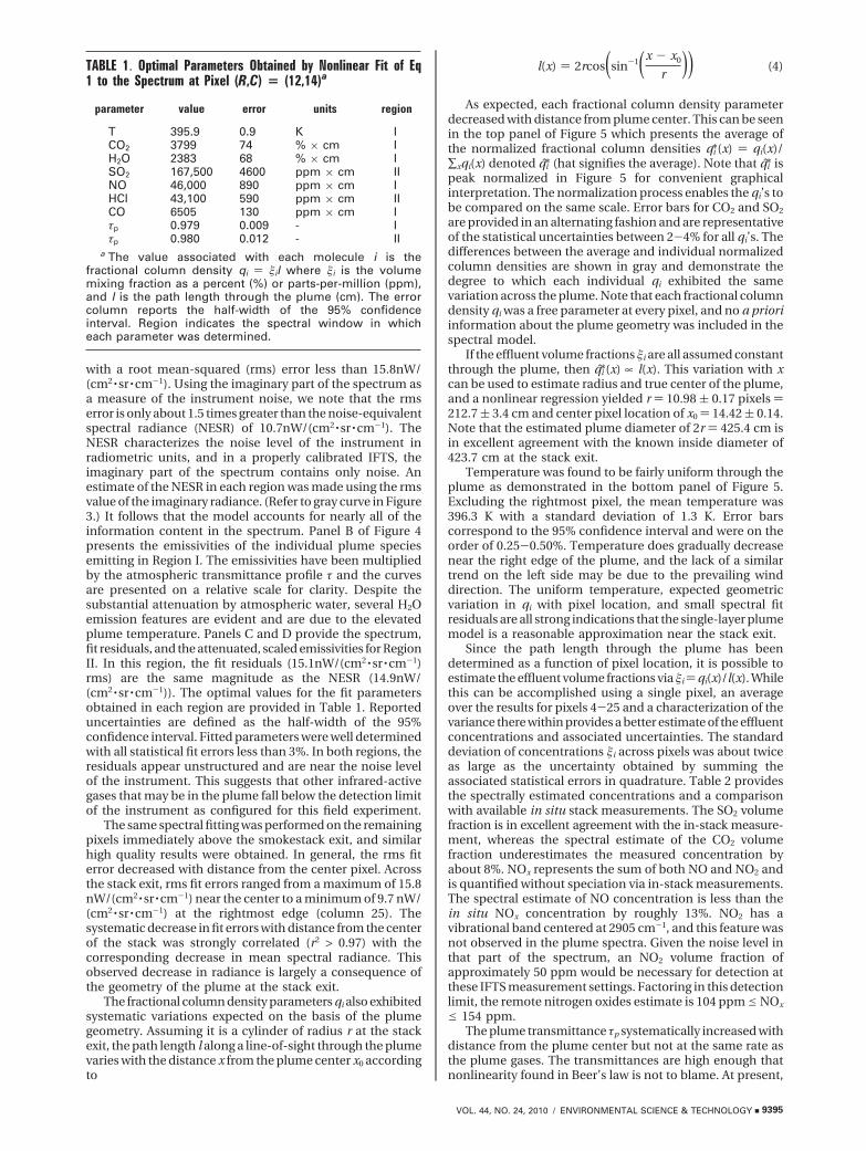
with a root mean-squared (rms) error less than 15.8nW/(cm2 · sr · cm-1). Using the imaginary part of the spectrum asa measure of the instrument noise, we note that the rmserror is only about 1.5 times greater than the noise-equivalentspectral radiance (NESR) of 10.7nW/(cm2 · sr · cm-1). TheNESR characterizes the noise level of the instrument inradiometric units, and in a properly calibrated IFTS, theimaginary part of the spectrum contains only noise. Anestimate of the NESR in each region was made using the rmsvalue of the imaginary radiance. (Refer to gray curve in Figure3.) It follows that the model accounts for nearly all of theinformation content in the spectrum. Panel B of Figure 4presents the emissivities of the individual plume speciesemitting in Region I. The emissivities have been multipliedby the atmospheric transmittance profile # and the curvesare presented on a relative scale for clarity. Despite thesubstantial attenuation by atmospheric water, several H2Oemission features are evident and are due to the elevatedplume temperature. Panels C and D provide the spectrum,fit residuals, and the attenuated, scaled emissivities for RegionII. In this region, the fit residuals (15.1nW/(cm2 · sr · cm-1)rms) are the same magnitude as the NESR (14.9nW/(cm2 · sr · cm-1)). The optimal values for the fit parametersobtained in each region are provided in Table 1. Reporteduncertainties are defined as the half-width of the 95%confidence interval. Fitted parameters were well determinedwith all statistical fit errors less than 3%. In both regions, theresiduals appear unstructured and are near the noise levelof the instrument. This suggests that other infrared-activegases that may be in the plume fall below the detection limitof the instrument as configured for this field experiment.

The same spectral fitting was performed on the remainingpixels immediately above the smokestack exit, and similarhigh quality results were obtained. In general, the rms fiterror decreased with distance from the center pixel. Acrossthe stack exit, rms fit errors ranged from a maximum of 15.8nW/(cm2 · sr · cm-1) near the center to a minimum of 9.7 nW/(cm2 · sr · cm-1) at the rightmost edge (column 25). Thesystematic decrease in fit errors with distance from the centerof the stack was strongly correlated (r2 > 0.97) with thecorresponding decrease in mean spectral radiance. Thisobserved decrease in radiance is largely a consequence ofthe geometry of the plume at the stack exit.

The fractional column density parameters qi also exhibitedsystematic variations expected on the basis of the plumegeometry. Assuming it is a cylinder of radius r at the stackexit, the path length l along a line-of-sight through the plumevaries with the distance x from the plume center x0 accordingto

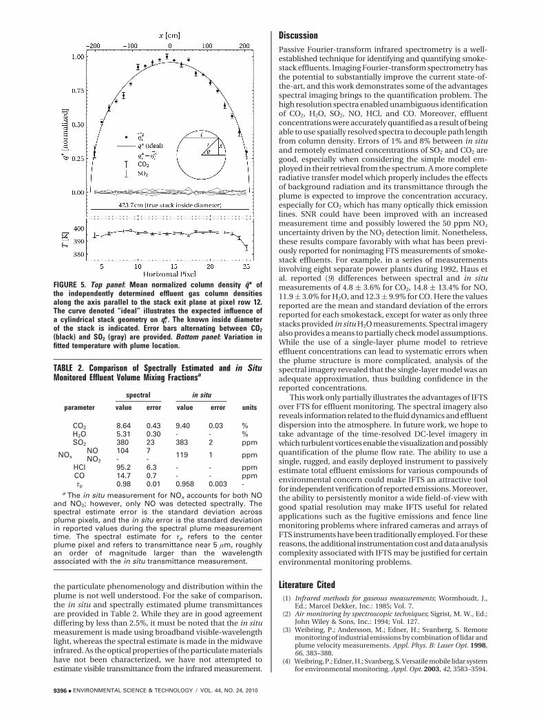
As expected, each fractional column density parameterdecreased with distance from plume center. This can be seenin the top panel of Figure 5 which presents the average ofthe normalized fractional column densities qi*(x) ) qi(x)/"xqi(x) denoted qi* (hat signifies the average). Note that qi* ispeak normalized in Figure 5 for convenient graphicalinterpretation. The normalization process enables the qi’s tobe compared on the same scale. Error bars for CO2 and SO2

are provided in an alternating fashion and are representativeof the statistical uncertainties between 2-4% for all qi’s. Thedifferences between the average and individual normalizedcolumn densities are shown in gray and demonstrate thedegree to which each individual qi exhibited the samevariation across the plume. Note that each fractional columndensity qi was a free parameter at every pixel, and no a prioriinformation about the plume geometry was included in thespectral model.

If the effluent volume fractions &i are all assumed constantthrough the plume, then qi*(x) # l(x). This variation with xcan be used to estimate radius and true center of the plume,and a nonlinear regression yielded r ) 10.98 ( 0.17 pixels )212.7 ( 3.4 cm and center pixel location of x0 ) 14.42 ( 0.14.Note that the estimated plume diameter of 2r ) 425.4 cm isin excellent agreement with the known inside diameter of423.7 cm at the stack exit.

Temperature was found to be fairly uniform through theplume as demonstrated in the bottom panel of Figure 5.Excluding the rightmost pixel, the mean temperature was396.3 K with a standard deviation of 1.3 K. Error barscorrespond to the 95% confidence interval and were on theorder of 0.25-0.50%. Temperature does gradually decreasenear the right edge of the plume, and the lack of a similartrend on the left side may be due to the prevailing winddirection. The uniform temperature, expected geometricvariation in qi with pixel location, and small spectral fitresiduals are all strong indications that the single-layer plumemodel is a reasonable approximation near the stack exit.

Since the path length through the plume has beendetermined as a function of pixel location, it is possible toestimate the effluent volume fractions via &i)qi(x)/l(x). Whilethis can be accomplished using a single pixel, an averageover the results for pixels 4-25 and a characterization of thevariance there within provides a better estimate of the effluentconcentrations and associated uncertainties. The standarddeviation of concentrations &i across pixels was about twiceas large as the uncertainty obtained by summing theassociated statistical errors in quadrature. Table 2 providesthe spectrally estimated concentrations and a comparisonwith available in situ stack measurements. The SO2 volumefraction is in excellent agreement with the in-stack measure-ment, whereas the spectral estimate of the CO2 volumefraction underestimates the measured concentration byabout 8%. NOx represents the sum of both NO and NO2 andis quantified without speciation via in-stack measurements.The spectral estimate of NO concentration is less than thein situ NOx concentration by roughly 13%. NO2 has avibrational band centered at 2905 cm-1, and this feature wasnot observed in the plume spectra. Given the noise level inthat part of the spectrum, an NO2 volume fraction ofapproximately 50 ppm would be necessary for detection atthese IFTS measurement settings. Factoring in this detectionlimit, the remote nitrogen oxides estimate is 104 ppmeNOx

e 154 ppm.The plume transmittance #p systematically increased with

distance from the plume center but not at the same rate asthe plume gases. The transmittances are high enough thatnonlinearity found in Beer’s law is not to blame. At present,

TABLE 1. Optimal Parameters Obtained by Nonlinear Fit of Eq1 to the Spectrum at Pixel (R,C) = (12,14)a

parameter value error units region

T 395.9 0.9 K ICO2 3799 74 % ! cm IH2O 2383 68 % ! cm ISO2 167,500 4600 ppm ! cm IINO 46,000 890 ppm ! cm IHCl 43,100 590 ppm ! cm IICO 6505 130 ppm ! cm I#p 0.979 0.009 - I#p 0.980 0.012 - II

a The value associated with each molecule i is thefractional column density qi ) &il where &i is the volumemixing fraction as a percent (%) or parts-per-million (ppm),and l is the path length through the plume (cm). The errorcolumn reports the half-width of the 95% confidenceinterval. Region indicates the spectral window in whicheach parameter was determined.

l(x) ) 2rcos(sin-1(x - x0

r )) (4)

VOL. 44, NO. 24, 2010 / ENVIRONMENTAL SCIENCE & TECHNOLOGY 9 9395

the particulate phenomenology and distribution within theplume is not well understood. For the sake of comparison,the in situ and spectrally estimated plume transmittancesare provided in Table 2. While they are in good agreementdiffering by less than 2.5%, it must be noted that the in situmeasurement is made using broadband visible-wavelengthlight, whereas the spectral estimate is made in the midwaveinfrared. As the optical properties of the particulate materialshave not been characterized, we have not attempted toestimate visible transmittance from the infrared measurement.

DiscussionPassive Fourier-transform infrared spectrometry is a well-established technique for identifying and quantifying smoke-stack effluents. Imaging Fourier-transform spectrometry hasthe potential to substantially improve the current state-of-the-art, and this work demonstrates some of the advantagesspectral imaging brings to the quantification problem. Thehigh resolution spectra enabled unambiguous identificationof CO2, H2O, SO2, NO, HCl, and CO. Moreover, effluentconcentrations were accurately quantified as a result of beingable to use spatially resolved spectra to decouple path lengthfrom column density. Errors of 1% and 8% between in situand remotely estimated concentrations of SO2 and CO2 aregood, especially when considering the simple model em-ployed in their retrieval from the spectrum. A more completeradiative transfer model which properly includes the effectsof background radiation and its transmittance through theplume is expected to improve the concentration accuracy,especially for CO2 which has many optically thick emissionlines. SNR could have been improved with an increasedmeasurement time and possibly lowered the 50 ppm NOx

uncertainty driven by the NO2 detection limit. Nonetheless,these results compare favorably with what has been previ-ously reported for nonimaging FTS measurements of smoke-stack effluents. For example, in a series of measurementsinvolving eight separate power plants during 1992, Haus etal. reported (9) differences between spectral and in situmeasurements of 4.8 ( 3.6% for CO2, 14.8 ( 13.4% for NO,11.9 ( 3.0% for H2O, and 12.3 ( 9.9% for CO. Here the valuesreported are the mean and standard deviation of the errorsreported for each smokestack, except for water as only threestacks provided in situ H2O measurements. Spectral imageryalso provides a means to partially check model assumptions.While the use of a single-layer plume model to retrieveeffluent concentrations can lead to systematic errors whenthe plume structure is more complicated, analysis of thespectral imagery revealed that the single-layer model was anadequate approximation, thus building confidence in thereported concentrations.

This work only partially illustrates the advantages of IFTSover FTS for effluent monitoring. The spectral imagery alsoreveals information related to the fluid dynamics and effluentdispersion into the atmosphere. In future work, we hope totake advantage of the time-resolved DC-level imagery inwhich turbulent vortices enable the visualization and possiblyquantification of the plume flow rate. The ability to use asingle, rugged, and easily deployed instrument to passivelyestimate total effluent emissions for various compounds ofenvironmental concern could make IFTS an attractive toolfor independent verification of reported emissions. Moreover,the ability to persistently monitor a wide field-of-view withgood spatial resolution may make IFTS useful for relatedapplications such as the fugitive emissions and fence linemonitoring problems where infrared cameras and arrays ofFTS instruments have been traditionally employed. For thesereasons, the additional instrumentation cost and data analysiscomplexity associated with IFTS may be justified for certainenvironmental monitoring problems.

Literature Cited(1) Infrared methods for gaseous measurements; Wormhoudt, J.,

Ed.; Marcel Dekker, Inc.: 1985; Vol. 7.(2) Air monitoring by spectroscopic techniques; Sigrist, M. W., Ed.;

John Wiley & Sons, Inc.: 1994; Vol. 127.(3) Weibring, P.; Andersson, M.; Edner, H.; Svanberg, S. Remote

monitoring of industrial emissions by combination of lidar andplume velocity measurements. Appl. Phys. B: Laser Opt. 1998,66, 383–388.

(4) Weibring, P.; Edner, H.; Svanberg, S. Versatile mobile lidar systemfor environmental monitoring. Appl. Opt. 2003, 42, 3583–3594.

FIGURE 5. Top panel: Mean normalized column density q* ofthe independently determined effluent gas column densitiesalong the axis parallel to the stack exit plane at pixel row 12.The curve denoted “ideal” illustrates the expected influence ofa cylindrical stack geometry on qi*. The known inside diameterof the stack is indicated. Error bars alternating between CO2(black) and SO2 (gray) are provided. Bottom panel: Variation infitted temperature with plume location.

TABLE 2. Comparison of Spectrally Estimated and in SituMonitored Effluent Volume Mixing Fractionsa

spectral in situ

parameter value error value error units

CO2 8.64 0.43 9.40 0.03 %H2O 5.31 0.30 - - %SO2 380 23 383 2 ppm

NOxNO 104 7 119 1 ppmNO2 - -

HCl 95.2 6.3 - - ppmCO 14.7 0.7 - - ppm#p 0.98 0.01 0.958 0.003 -

a The in situ measurement for NOx accounts for both NOand NO2; however, only NO was detected spectrally. Thespectral estimate error is the standard deviation acrossplume pixels, and the in situ error is the standard deviationin reported values during the spectral plume measurementtime. The spectral estimate for #p refers to the centerplume pixel and refers to transmittance near 5 µm, roughlyan order of magnitude larger than the wavelengthassociated with the in situ transmittance measurement.

9396 9 ENVIRONMENTAL SCIENCE & TECHNOLOGY / VOL. 44, NO. 24, 2010

(5) Sandsten, J.; Edner, H.; Svanberg, S. Gas visualization ofindustrial hydrocarbon emissions. Opt. Express 2004, 12, 1443–1451.

(6) Prengle, H. W.; Morgan, C. A.; Fang, C.-S.; Huang, L.-K.; Campani,P.; Wu, W. W. Infrared remote sensing and determination ofpollutants in gas plumes. Environ. Sci. Technol. 1973, 7, 417–423.

(7) Herget, W. F. Remote and cross-stack measurement of stackgas concentrations using a mobile FT-IR system. Appl. Opt.1982, 21, 635–641.

(8) Carlson, R. C.; Hayden, A. F.; Telfair, W. B. Remote observationsof effluents from small building smokestacks using FTIRspectroscopy. Appl. Opt. 1988, 27, 4952–4959.

(9) Haus, R.; Schafer, K.; Bautzer, W.; Heland, J.; Mosebach, H.;Bittner, H.; Eisenmann, T. Mobile Fourier-transform infraredspectroscopy monitoring of air pollution. Appl. Opt. 1994, 33,5682–5689.

(10) Hilton, M.; Lettington, A. H.; Mills, I. M. Quantitative analysisof remote gas temperatures and concentrations from theirinfrared emission spectra. Meas. Sci. Technol. 1995, 6, 1236–1241.

(11) Heland, J.; Schafer, K. Determination of major combustionproducts in aircraft exhausts by FTIR emission spectroscop.Atmos. Environ. 1998, 32, 3067–3072.

(12) Kricks, R. J.; Keely, J. A.; Spellicy, R. L.; Perry, S. H. Use ofopen-path FTIR monitoring for emission rate assessment ofindustrial area sources during winter conditions. Proc. SPIE1999.

(13) Schafer, K.; et al. Nonintrusive Optical Measurements ofAircraft Engine Exhaust Emissions and Comparison withStandard Intrusive Techniques. Appl. Opt. 2000, 39, 441-455.

(14) Smith, L. M.; Keefer, D. R.; Sudharsanan, S. I. Abel inversionusing transform techniques. J. Quant. Spectrosc. Radiat. Transfer1988, 39, 367–373.

(15) Yousefian, F.; Lallemand, M. Inverse radiative analysis of high-resolution infrared emission data for temperature and speciesprofiles recoveries in axisymmetric semi-transparent media. J.Quant. Spectrosc. Radiat. Transfer 1998, 60, 921–931.

(16) Moore, E. A.; Gross, K. C.; Bowen, S. J.; Perram, G. P.;Chamberland, M.; Farley, V.; Gagnon, J.-P.; Villemaire, A.Characterizing and overcoming spectral artifacts in imagingFourier-transform spectroscopy of turbulent exhaust plumes.Proc. SPIE 2009, 730416.

(17) Tremblay, P.; Gross, K. C.; Farley, V.; Chamberland, M.;Villemaire, A. Understanding and overcoming scene-changeartifacts in imaging Fourier-transform spectroscopy of turbulentjet engine exhaust. Proc. SPIE 2009, 74570F.

(18) Revercomb, H. E.; Bujis, H.; Howell, H. B.; LaPorte, D. D.; Smith,W. L.; Sromovsky, L. A. Radiometric calibration of IR Fouriertransform spectrometers: solution to a problem with the High-Resolution Interferometer Sounder. Appl. Opt. 1988, 27, 3210–3218.

(19) Chamberland, M.; Farley, V.; Tremblay, P.; Legault, J.-F.Performance model of imaging FTS as a standoff chemical agentdetection tool. Proc. SPIE 2004, 240–251.

(20) Farley, V.; Belzile, C.; Chamberland, M.; Legault, J.-F.; Schwantes,K. R. Development and testing of a hyperspectral imaginginstrument for field spectroscopy. Proc. SPIE 2004, 29–36.

(21) Chamberland, M.; Farley, V.; Vallieres, A.; Villemaire, A.;Belhumeur, L.; Giroux, J.; Legault, J.-F. High-performance field-portable imaging radiometric spectrometer technology forhyperspectral imaging applications. Proc. SPIE 2005, 59940N.

(22) Gross, K. C.; Tremblay, P.; Bradley, K. C.; Chamberland, M.;Farley, V.; Perram, G. P. Instrument calibration and lineshapemodeling for ultraspectral imagery measurements of industrialsmokestack emissions. Proc. SPIE 2010, 769516.

(23) Bradley, K. C. Ph.D. Thesis, Air Force Institute of Technology,AFIT/DS/ENP/09-S01, 2009.

(24) Rothman, L. S.; et al. The HITRAN molecular spectroscopicdatabase: edition of 2000 including updates through 2001. J.Quant. Spectrosc. Radiat. Transfer 2003, 82, 5–44.

(25) Herget, W. F.; Brasher, J. D. Remote measurement of gaseouspollutant concentrations using a mobile Fourier transforminterferometer system. Appl. Opt. 1979, 18, 3404–3420.

(26) The Infrared Handbook; Wolfe, W. L., Zissis, G. J., Eds.;Environmental Research Institute of Michigan: 1978.

(27) Witteman, W. J. The CO2 Laser; Springer-Verlag: 1987; Vol. 53.(28) Davis, S. P.; Abrams, M. C.; Brault, J. W. Fourier Transform

Spectrometry; Academic Press: 2001.(29) Modest, M. F. Radiative Heat Transfer; McGraw-Hill, Inc.: New

York, NY, 1993.(30) Thomas, G. E.; Stamnes, K. Radiative Transfer in the Atmosphere

and Ocean; Cambridge University Press: 2002.(31) Liu, L. H.; Tan, H. P.; Li, B. X. Influence of turbulent fluctuation

on reconstruction of temperature profile in axisymmetric freeflames. J. Quant. Spectrosc. Radiat. Transfer 2002, 73, 641-648.

(32) Clough, S.; Shephard, M.; Mlawer, E.; Delamere, J.; Iacono, M.;Cady-Pereira, K.; Boukabara, S.; Brown, P. Atmospheric radiativetransfer modeling: A summary of the AER codes. J. Quant.Spectrosc. Radiat. Transfer 2005, 91, 233–244.

ES101823Z

VOL. 44, NO. 24, 2010 / ENVIRONMENTAL SCIENCE & TECHNOLOGY 9 9397