NETWORKS AND HETEROGENEOUS MEDIA doi:10.3934/nhm.2010.5.xxc©American Institute of Mathematical SciencesVolume 5, Number 3, September 2010 pp. 1–xx

REMARKS ON DISCRETIZATIONS OF CONVECTION TERMS

IN HYBRID MIMETIC MIXED METHODS

Jerome Droniou

Universite Montpellier 2Institut de Mathematiques et de Modelisation de Montpellier, CC 051

Place Eugene Bataillon34095 Montpellier cedex 5, France

Abstract. We present different ways, coming from Finite Volume or MixedFinite Element frameworks, to discretize convection terms in Hybrid Finite Vol-ume, Mimetic Finite Difference and Mixed Finite Volume methods for ellipticequations. We compare them through several numerical tests, deducing somegeneric principles, depending on the situation, on the choice of an apropriatemethod and its parameters. We also present an adaptation to the Navier-Stokesequations, with a numerical tests in the case of the lid-driven cavity.

1. Introduction. The Hybrid Finite Volume (HFV), Mimetic Finite Difference(MFD) and Mixed Finite Volume (MFV) methods, developed in the last few years,aim at providing numerical schemes on very generic grids for diffusion equations ofthe kind

−div(Λ∇p) = f in Ω,p = 0 on ∂Ω,

(1)

where Ω is a polygonal open bounded subset of Rd (d ≥ 2) and Λ : Ω → Rd×d is abounded uniformly coercive (and usually symmetric) tensor.

These three methods basically come from two different communities: the MixedFinite Element community (MFD) and the Finite Volume community (HFV, MFV).It has recently been understood [9] that they are in fact only different presentations,based on the different takes and habits of each community, of a single discretizationtechnique, which can be named the “Hybrid Mimetic Mixed” (HMM) method.

Diffusion terms of the kind div(Λ∇p) appear in numerous models of physicalproblems, and their discretization on general grids is a complex problem whichalone justifies a large literature on development of methods for the plain diffusionequation (1). But many such models (the Navier-Stokes equations, miscible orimmiscible flows in porous media, etc.) also involve convection terms, and it istherefore important not only to study discretizations of pure diffusion equations, butalso to gather some understanding on how to handle convection-diffusion equations,

2000 Mathematics Subject Classification. Primary: 65N12, 65N30, 65M12, 65M60.Key words and phrases. Mixed finite volume, Hybrid finite volume, Mimetic finite difference,

Hybrid Mixed Mimetic method, convection-diffusion equation, convection-dominated problems,elliptic-parabolic coupled problems, flow in porous media.

This work was supported by GnR MoMaS CNRS/PACEN and Project VFSitCom (ANR-08-BLAN-0275-01).

1

2 JEROME DRONIOU

the model of those being

−div(Λ∇p) + div(V p) = f in Ω,p = 0 on ∂Ω

(2)

with V ∈ C1(Ω)d (since this equation is stationary, as usual we assume thatdiv(V ) ≥ 0). Of course, the discretization of div(V p) is not expected to besomething as complex as the discretization of div(Λ∇p), but it is well known thatconvection-diffusion equations can be quite tricky to properly approximate: differ-ent treatments of the convective term can be required depending on which process(the convection or the diffusion) dominates.

Mixed Finite Element and Finite Volume literatures both have developed tech-niques to handle convective terms; the HMM method being at the juncture of thesetwo literatures, it can be written in either one format and this mutability thusallows to try and incorporate into HMM schemes all those different handling ofconvection terms. The aim of this paper is precisely to present couplings of theHMM technique for pure diffusion equations with several FE or FV discretizationsof convection terms.

The plan is as follows: in the next section, we recall the HMM discretization ofpure diffusion equations (1), using two of its possible presentations (MFD and MFV)associated with the FE and FV views of the method. In Section 3, we use thesetwo presentations to couple the HMM method with FE- or FV-based discretizationsof the convective term, thus obtaining several schemes for the convection-diffusionequation (2); we very briefly state the theoretical results which can be proved onthese schemes, the details being provided in [2]. In Section 4 we present some nu-merical comparisons between these methods. The results are on the overall what isexpected, but some interesting insights can nevertheless be gained (for example, onthe scaling of the Scharfetter-Gummel method, or on the choice of cell or edge un-knowns in the upwindings). The model equation (2), although sometimes difficultto properly approximate, is a very simple convection-diffusion problem, which canhowever give pretty good ideas on how to discretize, using HMM methods, morecomplex convection-diffusion problems also involving heterogeneous and anisotropicdata (see e.g. [7], in which a slight variant of the HMM method has been applied to amodel of miscible flows in porous media). In Section 5, we present HMM discretiza-tions of the Navier-Stokes equation, which also involves diffusion and convectionterms; the classical situations of study of the Navier-Stokes equations only involvea homogeneous and isotropic diffusion term, but the model is a system of equationin which convective term is quite different from the one in (2) (being strongly non-linear), and some behaviors displayed by the solutions are quite different from theones which can be seen on the solutions to (2); a quick study of a classical test case(the lid driven cavity) therefore appears interesting to have a better grasp of thestrengths and weaknesses of the various HMM discretizations we consider in thiswork. Some concluding remarks are gathered in the last section of the paper.

2. The HMM discretization of pure diffusion equations.

2.1. Notations. The following definition gives the basic notations for the grids weconsider on Ω.

Definition 2.1. An admissible discretization of Ω is given by the triplet D =(M, E ,P), where :

CONVECTION TERMS IN HMM METHODS 3

• M, the cells (or control volumes) of the mesh, is a finite family of non-emptyopen polygonal disjoint subsets of Ω such that Ω = ∪K∈MK;

• E , the edges (faces in 3D) of the mesh, is a finite family of non-empty opendisjoint subsets σ of Ω such that for all σ ∈ E there exists an affine hyperplaneA of Rd and a cell K ∈ M such that σ ⊂ ∂K ∩ A. We also assume that forall K ∈ M there exists EK ⊂ E such that ∂K = ∪σ∈Eσ and, for all σ ∈ E ,either σ ⊂ ∂Ω or σ ∈ EK ∩ EL for some pair of elements K, L ∈ M;

• P = (xK)K∈M is a family of points of Ω indexed by M, such that each meshcell K is star-shaped with respect to xK .

The set of edges σ contained in ∂Ω is denoted by Eext, and we let Eint = E\Eext

denote the interior edges. Two control volumes K and L which share an edge arecalled neighbors; |K| and |σ| respectively denote the d-dimensional and the (d− 1)-dimensional measures of the cell K and the edge σ. If σ ∈ EK , nK,σ is the unitnormal to σ outward K.

We define HM as the set of functions Ω → R which are piecewise constant onM (the value of q ∈ HM on K is denoted by qK), and FD is the set of families ofreal numbers (FK,σ)K∈M,σ∈EK

which satisfy the following conservativity property:

for all K and L neighbors, for all σ ∈ EK ∩ EL : FK,σ + FL,σ = 0. (3)

2.2. Scheme. The HMM method for the diffusion equation (1) can be introducedin three different but equivalent ways [9], coming from three different points ofview: in a manner similar to the Mixed Finite Element method (MFD), using avariational formulation of the problem based on discrete gradients (HFV) or writinga flux-based finite volume formulation (MFV). We briefly describe here the first andthird presentations, which will be useful to introduce the various discretizations ofthe convection term in the next section, and we refer the reader to [4, 9, 10, 13] formore detailed constructions of the method.

In the MFD view of the HMM method, a discrete divergence operator is firstdefined: for all G ∈ FD, DIV(G) ∈ HM is given by

(DIV(G))K =1

|K|

∑

σ∈EK

|σ|GK,σ

and, for each control volume K, a local scalar product [·, ·]K , acting on the re-strictions to EK of elements in FD, is chosen such that the following consistencyproperty holds (this is the discrete counterpart of the usual Stokes formula):

∀G ∈ FD , ∀q affine function :

[(ΛK∇q)I , G]K +

∫

K

q(DIV(G))K =∑

σ∈EK

GK,σ

∫

σ

q, (4)

where ΛK = 1|K|

∫

KΛ and the interpolation wI of a sufficiently regular vector field

w is defined by (w)IK,σ = 1

|σ|

∫

σw · nK,σ.

Remark 2.2. To prove the convergence of the method, the local scalar products[·, ·]K are also assumed to satisfy the following estimates:

∀G ∈ FD , ∀K ∈ M : C∗

∑

σ∈EK

|K|(GK,σ)2 ≤ [G, G]K ≤ C∗∑

σ∈EK

|K|(GK,σ)2 (5)

with C∗, C∗ > 0 not depending on the mesh in the family along which the conver-gence is studied.

4 JEROME DRONIOU

Defining the scalar product [·, ·]FDon FD as the sum of all the local scalar

products, i.e. [F, G]FD=

∑

K∈M[F, G]K , and [·, ·]HMas the usual L2(Ω) scalar

product, the HMM scheme for (1) consists in writing a Mixed Finite Element-likeformulation using these scalar products: find (p, F ) ∈ HM ×FD such that

∀G ∈ FD : [F, G]FD− [p,DIV(G)]HM

= 0 , (6)

∀q ∈ HM : [DIV(F ), q]HM= (f, q)L2(Ω). (7)

As with the classical Mixed Finite Element method, it is possible to hybridizethis scheme by introducing edge unknowns pE = (pσ)σ∈E (local eliminations thenallow to write the entire system using only pE). These edge unknowns are usefulto present the MFV approach of the HMM method; we first define a discrete cellgradient from the fluxes:

vK(F ) = −1

|K|Λ−1

K

∑

σ∈EK

|σ|FK,σ(xσ − xK), (8)

where xσ is the center of gravity of σ (and xK is the point corresponding to thechosen discretization D of Ω); if FK,σ is an approximation of 1

|σ|

∫

σ−Λ∇p·nK,σ, then

vK(F ) is indeed an approximation of ∇p on K. Letting HE,0 be the space of edgevalues qE = (qσ)σ∈E such that qσ = 0 whenever σ ∈ Eext, the HMM scheme consistsin imposing a relation inside each cell between the flux, cell and edge unknowns,and in writing the physical flux balance: find (p, pE , F ) ∈ HM × HE,0 × FD suchthat

∀K ∈ M , ∀G ∈ FD :∑

σ∈EK

|σ|GK,σ(pK − pσ)

= |K|vK(F ) · ΛKvK(G) + TK(G)TBKTK(F ) , (9)

∀K ∈ M :∑

σ∈EK

|σ|FK,σ =

∫

K

f , (10)

where TK(F ) = (TK,σ(F ))σ∈EKwith TK,σ(F ) = FK,σ + ΛKvK(F ) · nK,σ and BK

is a symmetric positive definite matrix of size Card(EK) (we see that TK(F ) = 0whenever (FK,σ)σ∈EK

are the genuine fluxes of a given vector ξ, i.e. FK,σ = ΛKξ ·nK,σ, and the term TK(G)T

BKTK(F ) is thus a stabilization term which vanishesas F approximates the genuine fluxes of the exact solution).

Remark 2.3. Rigorously speaking, (6)–(7) and (9)–(10) are equivalent only if thepoints (xK)K∈M are chosen as the centers of gravity of the cells. In general, (4) hasto be generalized a little bit in order to preserve the equivalence; this generalizationis at the core of the unified HMM view of the method, see [9].

3. Various discretizations of the convection term.

3.1. Using mixed finite element techniques. A first idea to discretize the con-vective term in (1) is to put this equation into a mixed weak formulation; H(div, Ω)being the classical space of square-integrable vector fields with square-integrabledivergence, a weak formulation for (2) is: find (p, F ) ∈ L2(Ω)×H(div, Ω) such that

∀w ∈ H(div, Ω) : (Λ−1F,w)L2(Ω) − (p, div(w))L2(Ω)

− (Λ−1V p,w)L2(Ω) = 0 , (11)

∀q ∈ L2(Ω) : (div(F ), q)L2(Ω) = (f, q)L2(Ω) (12)

CONVECTION TERMS IN HMM METHODS 5

(the first equation states that F = −Λ∇p + V p, and the second equation thatdiv(F ) = f).

If w and z are regular vector fields then, taking G = wI and q an affine functionsuch that ∇q = Λ−1

K1

|K|

∫

Kz in (4), since (DIV(G))K = 1

|K|

∫

Kdiv(w) = div(w) +

O(diam(K)) on K, we obtain, thanks to (5),

[zI ,wI ]K +

∫

K

qdiv(w)+O(|K|diam(K)) =∑

σ∈EK

GK,σ

∫

σ

q =∑

σ∈EK

∫

σ

w ·nK,σq(xσ)

(we use the fact that q is affine, so that∫

σq = |σ|q(xσ)). Integrating by part the

second term, we find

[zI ,wI ]K =

∫

K

∇q · w +∑

σ∈EK

∫

σ

w · nK,σ(q(xσ) − q) + O(|K|diam(K)).

We then notice that ∇q = Λ−1K z+O(diam(K)) on K, that w = w(xσ)+O(diam(K))

and q(xσ)− q = O(diam(K)) on σ, that |σ|diam(K) = O(|K|) and that∫

σ(q(xσ)−

q) = 0 to obtain

[zI ,wI ]K =

∫

K

Λ−1K z · w + O(|K|diam(K)).

Assuming that Λ is constant inside each control volume K, this justifies the followingapproximation of the convective term in (11):

(Λ−1V p,w)L2(Ω) =∑

K∈M

∫

K

Λ−1K V p·w ≈

∑

K∈M

pK

∫

K

Λ−1K V ·w ≈

∑

K∈M

pK [V I , G]K

where we have taken G = wI .The resulting HMM scheme for the full equation (2), proposed and studied in

[5], is then: find (p, F ) ∈ HM ×FD such that

∀G ∈ FD : [F, G]FD− [p,DIV(G)]HM

−∑

K∈M

pK [V I , G]K = 0 , (13)

∀q ∈ HM : [DIV(F ), q]HM= (f, q)L2(Ω). (14)

It has been proved in [5] that, under usual assumptions on the grid regularityand if the solution to (2) belongs to H2(Ω), an order 1 error estimate for p and thefluxes holds in natural norms (the L2 norm for the p, the norm on FD induced by[·, ·]FD

for the fluxes). Moreover, under stronger regularity assumptions on the grid,domain, source and velocity terms, a superconvergence of p can also be theoreticallyproved.

In case of strong convection, it turns out that (13)–(14), though still theoreticallyconvergent, can provide very oscillating solutions on coarse meshes. It is thenpossible to improve its behaviour by adding a stabilization term which consists inpenalizing the jumps of the solution: we define JD(p) ∈ HM by

JD(p)K =ζ

2|K|

∑

σ∈EK

|σ| |(V I)K,σ| (pK − pL)

(where L is the cell on the other side of σ, and pL = 0 if σ ∈ Eext), with ζ > 0 whichcan be chosen in order to control the strength of the penalization, and we replace(14) with

∀q ∈ HM : [DIV(F ) + JD(p), q]HM= (f, q)L2(Ω). (15)

6 JEROME DRONIOU

Obviously, the choice ζ = 0 gives back the original method (13)–(14).

3.2. Using finite volume techniques. The principle of Finite Volume discretiza-tions of the term div(V p) in (2) is to integrate it on a cell and use Stokes’ formula:

∫

K

div(V p) =∑

σ∈EK

∫

σ

pV · nK,σ =:∑

σ∈EK

|σ|Fc(p)K,σ.

The next step is to approximate Fc(p)K,σ = 1|σ|

∫

σpV · nK,σ using the available

unknowns, i.e. the cell unknowns (pK)K∈M in general; there are several possibleclassical choices. In the following, we let VK,σ = 1

|σ|

∫

σV · nK,σ and denote by L

the control volume on the other side of σ ∈ EK (or pL = 0 if σ ∈ EK ∩ Eext).

• Centered flux:

Fc(p)K,σ = VK,σ

pK + pL

2. (16)

• Upwind flux:

Fc(p)K,σ =

VK,σpK if VK,σ ≥ 0 ,VK,σpL if VK,σ < 0.

(17)

• Scharfetter-Gummel flux, scaled with the local diffusion:

Fc(p)K,σ =µσ

dσ

[

A

(

dσ

µσ

VK,σ

)

pK − A

(

−dσ

µσ

VK,σ

)

pL

]

(18)

where dσ is the sum of the orthogonal distances between σ and xK and be-tween σ and xL, A(s) = −s

e−s−1 − 1 and µσ = min(1, minSp(ΛK) ∪ Sp(ΛL))

(see Sections 4.1 and 4.2.2 for some comments on the use of µσ as a scalingparameter).

A HMM scheme for (2) can then be obtained from (9)–(10) by adding the con-vective fluxes to the flux balance equation: find (p, pE , F ) ∈ HM ×HE,0 ×FD suchthat

∀K ∈ M , ∀G ∈ FD :∑

σ∈EK

|σ|GK,σ(pK − pσ)

= |K|vK(F ) · ΛKvK(G) + TK(G)TBKTK(F ) , (19)

∀K ∈ M :∑

σ∈EK

|σ| (FK,σ + Fc(p)K,σ) =

∫

K

f , (20)

with Fc defined by one of the preceding choices (16), (17) or (18).All these expressions of the convective fluxes use the two values on either side of σ

as in the classical 2-point Finite Volume method (in which the primary unknowns arethe cell unknowns, see [12]). However, as noticed above, HMM methods naturallyprovide an unknown for p on each edge, which could be used instead of the cellunknown on the other side; for example, in the case of an upwind discretization,the discrete convective flux (17) can be replaced with

Fc(p, pE)K,σ =

VK,σpK if VK,σ ≥ 0 ,VK,σpσ if VK,σ < 0

(21)

(edge-based variants of the centered and Scharfetter-Gummel discretizations (16)and (18) can also be devised). Whereas the fluxes (17) are conservative, this isnot the case for the fluxes Fc(p, pE) defined by (21); since the conservativity of theglobal (diffusive+convective) fluxes is still expected to hold, (3) has to be relaxed

CONVECTION TERMS IN HMM METHODS 7

and, with the choice (21), the HMM scheme is thus: find (p, pE) ∈ HM × HE,0 anda set of real numbers F = (FK,σ)K∈M, σ∈EK

such that

∀K, L neighboring cells, ∀σ ∈ EK ∩ EL :

FK,σ + Fc(p, pE)K,σ + FL,σ + Fc(p, pE)L,σ = 0 ,(22)

∀K ∈ M , ∀(GK,σ)σ∈EK∈ RCard(EK) :

∑

σ∈EK

|σ|GK,σ(pK − pσ) = |K|vK(F ) · ΛKvK(G) + TK(G)TBKTK(F ) , (23)

∀K ∈ M :∑

σ∈EK

|σ| (FK,σ + Fc(p, pE)K,σ) =

∫

K

f. (24)

3.3. A word on the theoretical study. As shown in [2], all these HMM schemesfor convection-diffusion equations (i.e. the stabilized MFE-based scheme [(13),(15)],the FV-based methods with cell unknowns (19)–(20) and the FV-based methodswith cell and edge unknowns (22)–(24)) can be written in a unified presentationwhich allows to make a single theoretical study encompassing them all, and otherpossible methods.

In particular, theoretical proofs of convergence (without regularity assumptionon the solution to the PDE) and first order error estimates (when the solution to thePDE belongs to H2) are established in [2], under usual assumptions on the grids.

4. Numerical results. We provide here some numerical results on the schemes,some of them leading to what we believe to be interesting and new comments onsome choices of the discretization of the convection term.

4.1. Orders of convergence. Some rates of convergence for the preceding meth-ods are provided in [2], but only in the case of isotropic and homogeneous cases(Λ = νId and V constant). We complete here those results by looking at the ratesof convergence in the following anisotropic heterogeneous case: we consider (2) with

• Ω = (0, 1)2,• Λ(x, y) the diffusion tensor given by a 2πx rotation of the diagonal matrix

νdiag(2, 1) for some ν > 0, i.e.

Λ(x, y) =

ν

(

cos(2πx) − sin(2πx)sin(2πx) cos(2πx)

) (

2 00 1

) (

cos(2πx) − sin(2πx)sin(2πx) cos(2πx)

)−1

,(25)

• V the divergence-free vector field V (x, y) = 10(−y, x),• f the source term corresponding to the exact solution p(x, y) = x(1 − x)ey.

If ν is not small (say ν = 1), this problem is mostly in diffusive regime; for smallν, the convection dominates. We implement the schemes using refinements of thegrid presented in Figure 1-(a): each primordial, triangular or quadrangular, cell isdivided into a certain number of cells of the same nature, obtained by cutting eachedge into n segments; Figure 1-(b) shows the refinement corresponding to n = 10(the grids used in the tests correspond to n = 25, n = 50, n = 100, n = 150 andn = 200 and are respectively made of 5625, 22500, 90000, 202500 and 360000 cells).

8 JEROME DRONIOU

(a) n = 1 (b) n = 10

Figure 1. Two elements of the family of grids used to computethe rates of convergence.

The quantities of interest are the relative errors ep and e∇p, in L2 norms, of pand ∇p, i.e.

ep =||p − pM||L2(Ω)

||pM||L2(Ω)and e∇p =

||v(F ) − (∇p)M||L2(Ω)

||(∇p)M||L2(Ω)

where p is the approximate piecewise constant solution given by the consideredscheme, pM = (p(xK))K∈M and (∇p)M = (∇p(xK))K∈M are piecewise constantprojections of the exact solution to (2) and its gradient, and v(F ) is the approximategradient defined by (8).

In Figure 2 we present the convergence graphs obtained in the diffusive regimeν = 1, with various discretizations of the convection: the FV-upwind method basedon (21), the FV-Scharfetter-Gummel method based on the edge-version of (18) (i.e.with pL replaced by pσ), the FV-centered method based on (16) but also replacing pL

with pσ, the FE-like method (13)–(14) and the stabilized FE-like method [(13),(15)]with ζ = 1.

These results show a super-convergence (order 2) of p for all the schemes exceptthe FV-upwind scheme and the stabilized FE-like scheme (which only exhibits anorder 1 convergence), and an order 1 convergence of the discrete gradient for all theschemes. Other test cases in diffusive regime give similar outputs, but the relativepositions of the three schemes showing a superconvergence for p may change (ina numerical test of [2], the FE-like discretization gives slightly better results thanthe two others). These behaviors are somewhat expected, and correspond to whatis observed when these techniques of discretization of the convective term are usedalongside other kinds of schemes for diffusion operators.

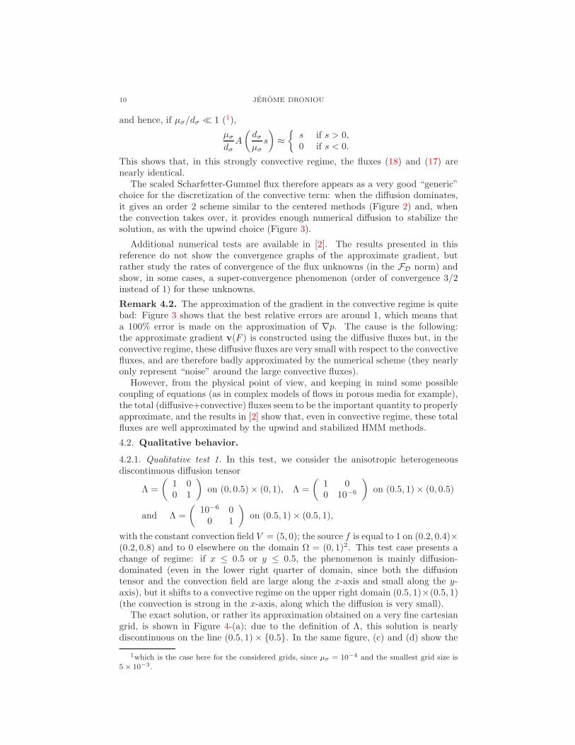
In Figure 3, we present the results in the convection-dominated case: we takeν = 10−4 in (25). Here again, the results correspond to the expectations: the FV-centered discretization nearly provides, as the mesh size goes to 0, a second order ofconvergence for p, but with very large errors, whereas the FV-upwind and stabilizedFE-like schemes still have a convergence rate of order 1, but gives an acceptablenumerical solution. Also as expected, the convergence of the approximate gradientis very slow at the available mesh sizes.

CONVECTION TERMS IN HMM METHODS 9

10−2

10−3

10−4

10−5

10−1 10−2 10−3

10−1 10−2 10−3

e∇p

10−1

10−2

10−3

10−4

ep

Legend: © FV-upwind, FV-Scharfetter-Gummel, FV-centered, ⋆ FE-like, +stabilized FE-like.

Figure 2. Rates of convergence in the diffusive regime (ν = 1 in(25)): graph in log-log scale of the errors with respect to the sizeh of the mesh (reference slopes: h and h2).

Remark 4.1. We do not include, in the convective regime, the results obtainedwith the non-stabilized FE-like method since the corresponding scheme gives a veryunstable solution (the error is huge on the the grids we consider here)

A more interesting remark can be made on the Scharfetter-Gummel discretiza-tion: the corresponding solution is nearly indistinguishable from the solution pro-vided by the upwind scheme; this is in fact completely natural if we remember thedefinition of the scaling parameter µσ in (18): we have

µσ

dσ

A

(

dσ

µσ

s

)

=−s

exp(− dσ

µσ

s) − 1−

µσ

dσ

10 JEROME DRONIOU

and hence, if µσ/dσ ≪ 1 (1),

µσ

dσ

A

(

dσ

µσ

s

)

≈

s if s > 0,0 if s < 0.

This shows that, in this strongly convective regime, the fluxes (18) and (17) arenearly identical.

The scaled Scharfetter-Gummel flux therefore appears as a very good “generic”choice for the discretization of the convective term: when the diffusion dominates,it gives an order 2 scheme similar to the centered methods (Figure 2) and, whenthe convection takes over, it provides enough numerical diffusion to stabilize thesolution, as with the upwind choice (Figure 3).

Additional numerical tests are available in [2]. The results presented in thisreference do not show the convergence graphs of the approximate gradient, butrather study the rates of convergence of the flux unknowns (in the FD norm) andshow, in some cases, a super-convergence phenomenon (order of convergence 3/2instead of 1) for these unknowns.

Remark 4.2. The approximation of the gradient in the convective regime is quitebad: Figure 3 shows that the best relative errors are around 1, which means thata 100% error is made on the approximation of ∇p. The cause is the following:the approximate gradient v(F ) is constructed using the diffusive fluxes but, in theconvective regime, these diffusive fluxes are very small with respect to the convectivefluxes, and are therefore badly approximated by the numerical scheme (they nearlyonly represent “noise” around the large convective fluxes).

However, from the physical point of view, and keeping in mind some possiblecoupling of equations (as in complex models of flows in porous media for example),the total (diffusive+convective) fluxes seem to be the important quantity to properlyapproximate, and the results in [2] show that, even in convective regime, these totalfluxes are well approximated by the upwind and stabilized HMM methods.

4.2. Qualitative behavior.

4.2.1. Qualitative test 1. In this test, we consider the anisotropic heterogeneousdiscontinuous diffusion tensor

Λ =

(

1 00 1

)

on (0, 0.5)× (0, 1), Λ =

(

1 00 10−6

)

on (0.5, 1) × (0, 0.5)

and Λ =

(

10−6 00 1

)

on (0.5, 1) × (0.5, 1),

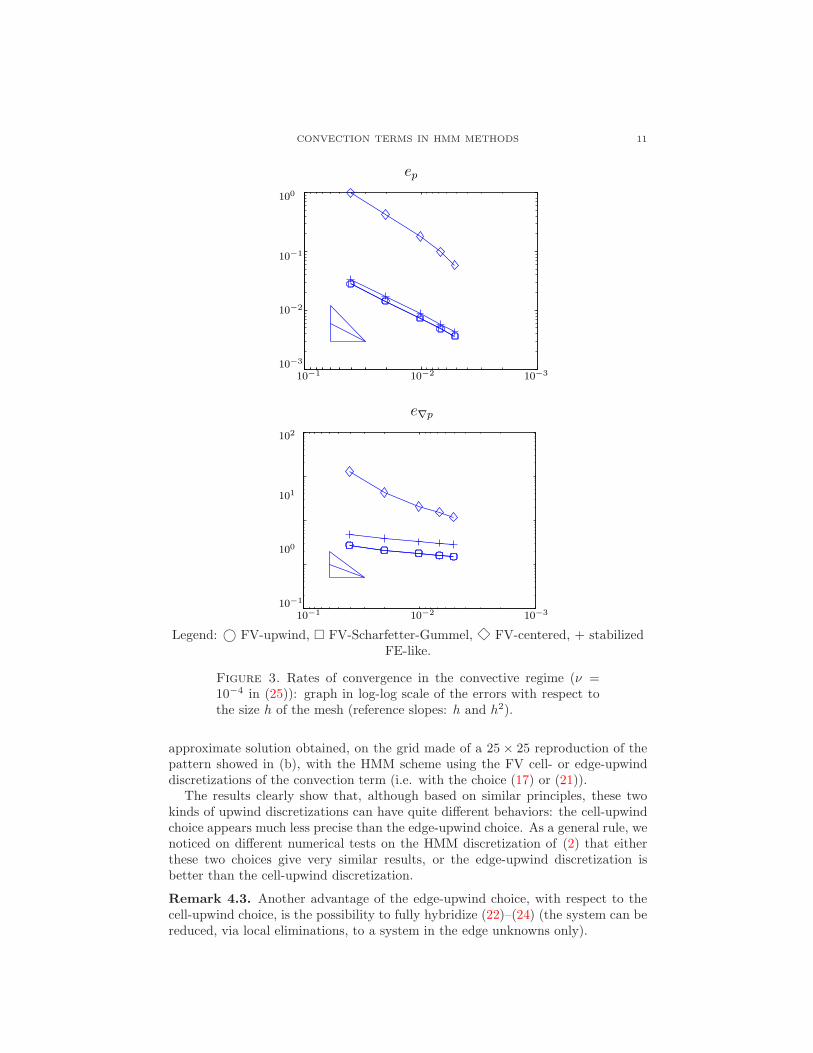
with the constant convection field V = (5, 0); the source f is equal to 1 on (0.2, 0.4)×(0.2, 0.8) and to 0 elsewhere on the domain Ω = (0, 1)2. This test case presents achange of regime: if x ≤ 0.5 or y ≤ 0.5, the phenomenon is mainly diffusion-dominated (even in the lower right quarter of domain, since both the diffusiontensor and the convection field are large along the x-axis and small along the y-axis), but it shifts to a convective regime on the upper right domain (0.5, 1)×(0.5, 1)(the convection is strong in the x-axis, along which the diffusion is very small).

The exact solution, or rather its approximation obtained on a very fine cartesiangrid, is shown in Figure 4-(a); due to the definition of Λ, this solution is nearlydiscontinuous on the line (0.5, 1) × 0.5. In the same figure, (c) and (d) show the

1which is the case here for the considered grids, since µσ = 10−4 and the smallest grid size is5 × 10−3.

CONVECTION TERMS IN HMM METHODS 11

10−1 10−2 10−3

100

10−1

10−2

10−3

10−1 10−2 10−3

102

101

100

10−1

e∇p

ep

Legend: © FV-upwind, FV-Scharfetter-Gummel, FV-centered, + stabilizedFE-like.

Figure 3. Rates of convergence in the convective regime (ν =10−4 in (25)): graph in log-log scale of the errors with respect tothe size h of the mesh (reference slopes: h and h2).

approximate solution obtained, on the grid made of a 25 × 25 reproduction of thepattern showed in (b), with the HMM scheme using the FV cell- or edge-upwinddiscretizations of the convection term (i.e. with the choice (17) or (21)).

The results clearly show that, although based on similar principles, these twokinds of upwind discretizations can have quite different behaviors: the cell-upwindchoice appears much less precise than the edge-upwind choice. As a general rule, wenoticed on different numerical tests on the HMM discretization of (2) that eitherthese two choices give very similar results, or the edge-upwind discretization isbetter than the cell-upwind discretization.

Remark 4.3. Another advantage of the edge-upwind choice, with respect to thecell-upwind choice, is the possibility to fully hybridize (22)–(24) (the system can bereduced, via local eliminations, to a system in the edge unknowns only).

12 JEROME DRONIOU

(a) Exact solution (b) Grid pattern

(c) Cell upwind (d) Edge upwind

Figure 4. Qualitative test 1, with a change of regime: compar-ison between the cell and edge upwind choices (the approximatesolutions (c) and (d) are obtained on the grid made of a 25 × 25reproduction of the pattern (b)).

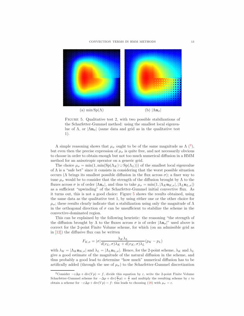
4.2.2. Qualitative test 2. In this test, we study in more depth the scaling used inthe Scharfetter-Gummel convective flux (18).

The Scharfetter-Gummel scheme has been developed for an homogeneous isotro-pic material (Λ = Id), in dimension 1 or for the standard 2-point Finite Volumescheme, to give a simultaneous approximation of the diffusion and convection fluxes[16, 6]. One can extract a “purely convective” flux from this method by consideringthe 2-point Finite Volume Scharfetter-Gummel schme for −∆p + div(V p) = f andcrudely removing the 2-point approximation of the diffusive flux: this leads to taking

Fc(p)K,σ =1

dσ

(A (−dσVK,σ) pK − A (dσVK,σ) pL) . (26)

However, this simple construction is completely unstable in convection-dominatedcases and it has to be scaled using some coefficient µσ, which takes into account thelocal diffusivity of the PDE, and writing (18) instead of (26). As we saw above, ifµσ is close to 0, its use ensures that the Scharfetter-Gummel method nearly boilsdown to an upwind (and thus very stable, although quite diffusive) scheme.

CONVECTION TERMS IN HMM METHODS 13

(a) min Sp(Λ) (b) |Λnσ|

Figure 5. Qualitative test 2, with two possible stabilizations ofthe Scharfetter-Gummel method: using the smallest local eigenva-lue of Λ, or |Λnσ| (same data and grid as in the qualitative test1).

A simple reasoning shows that µσ ought to be of the same magnitude as Λ (2),but even then the precise expression of µσ is quite free, and not necessarily obviousto choose in order to obtain enough but not too much numerical diffusion in a HMMmethod for an anisotropic operator on a generic grid.

The choice µσ = min(1, min(Sp(ΛK) ∪ Sp(ΛL))) of the smallest local eigenvalueof Λ is a “safe bet” since it consists in considering that the worst possible situationoccurs (Λ brings its smallest possible diffusion in the flux across σ); a finer way totune µσ would be to consider that the strength of the diffusion brought by Λ to thefluxes across σ is of order |Λnσ|, and thus to take µσ = min(1, |ΛKnK,σ|, |ΛLnL,σ|)as a sufficient “upwinding” of the Scharfetter-Gummel initial convective flux. Asit turns out, this is not a good choice: Figure 5 shows the results obtained, usingthe same data as the qualitative test 1, by using either one or the other choice forµσ; these results clearly indicate that a stabilization using only the magnitude of Λin the orthogonal direction of σ can be unsufficient to stabilize the scheme in theconvective-dominated region.

This can be explained by the following heuristic: the reasoning “the strength ofthe diffusion brought by Λ to the fluxes across σ is of order |Λnσ|” used above iscorrect for the 2-point Finite Volume scheme, for which (on an admissible grid asin [12]) the diffusive flux can be written

FK,σ = |σ|λKλL

d(xL, σ)λK + d(xK , σ)λL

(pK − pL)

with λK = |ΛKnK,σ| and λL = |ΛLnL,σ|. Hence, for the 2-point scheme, λK and λL

give a good estimate of the magnitude of the natural diffusion in the scheme, andthus probably a good lead to determine “how much” numerical diffusion has to beartifically added (through the use of µσ) to the Scharfetter-Gummel discretization

2Consider −ε∆p + div(V p) = f , divide this equation by ε, write the 2-point Finite Volume

Scharfetter-Gummel scheme for −∆p + div(Vε

p) = fε

and multiply the resulting scheme by ε to

obtain a scheme for −ε∆p + div(V p) = f : this leads to choosing (18) with µσ = ε.

14 JEROME DRONIOU

of the convective term in order to stabilize the global method. But for HMMschemes, the expression of the diffusive flux is less straightforward and involves allthe directions, not only the orthogonal direction to the edge: (9) shows that theexpression of FK,σ involves all the (pK − pσ′)σ′∈EK

, not only pK − pσ. . .

5. Application to Navier-Stokes equations. It might be interesting to look atthe various discretization of convection terms in HMM schemes for more complexproblems than the pure convection-diffusion equation. The upwind technique, forexample, has been used in conjunction with a variant of the HMM method (re-placing TK(F ) by FK and choosing a diagonal BK in (9)) in [7] for a non-linearelliptic-parabolic system of equations modeling miscible flows in porous media; thissituation is quite close to the one described by our basic equation (2), and theconclusions of the previous numerical tests can give pretty good insights on how tochoose the discretization of the convection term, depending on the expected regime.

We want to study here the previous HMM methods for a different kind of non-linear model, involving diffusion and convection operators but in an isotropic ho-mogeneous situation and leading to quite different behaviors than the behaviorsdisplayed by the solution to (2): the Navier-Stokes equation

−∆u + (u · ∇)u + ∇p = f in Ω,div(u) = 0 in Ω,u = 0 on ∂Ω,∫

Ω

p = 0,

(27)

where u : Ω → Rd is the velocity field and p : Ω → R the pressure (we present theequation with an homogeneous boundary condition for simplicity).

The same variant as above of the HMM method has been used in [11] to discretizethis equation (and its transient form), using a kind of centered discretization ofthe non-linear convective term (u · ∇)u, but it is quite easy to write the genuineHMM scheme for this equation, using any of the techniques from Section 3 for thediscretization of the non-linear term. The presentation of this method for Navier-Stokes equations, and above all the numerical study of various possible choices forthe discretization of the convective term, is not made in [2] or [11] and some of theconclusions we draw below are therefore new.

Remark 5.1. Note that it is possible to modify, at some cost (large stencil, someinstabilities in case of heterogeneities...), the HMM method in order to obtain a cell-centered scheme; it has been done in [13] for the pure scalar diffusion equation, andin [8] for the Navier-Stokes equation, with two possible choices for the discretizationof the convection term (centered or upwind, but all other choices are easily usable).

5.1. The discretization. The unknowns associated with the HMM discretizationof (27) are the cell and edge vector velocities u = (uK)K∈M ∈ Hd

M and uE =(uσ)σ∈E ∈ Hd

E,0, the vector velocity fluxes F = (FK,σ)K∈M , σ∈EK∈ Fd

D,nc and

the scalar pressure p = (pK)K∈M ∈ HM (we denote by FD,nc the space of possibly

non-conservative families of real numbers (FK,σ)K∈M , σ∈EK). The link between the

discrete velocity and its fluxes is made by using the matrices

vK(FK) = −1

|K|

∑

σ∈EK

|σ|FK,σ ⊗ (xσ − xK)

CONVECTION TERMS IN HMM METHODS 15

and by writing

∀K ∈ M , ∀G ∈ FdD,nc :

∑

σ∈EK

|σ|GK,σ · (uσ − uK)

=

d∑

i=1

(

vK(FK)i · vK(GK)i + TK((GK)i)T

BK,iTK((FK)i))

(28)

where vK(FK)i is the i-th line of the matrix vK(FK), TK((FK)i) =(

(FK,σ)i +

vK(FK)i ·nK,σ

)

σ∈Eand BK,i is a symmetric positive definite Card(EK)×Card(EK)

matrix.The incompressibility condition div(u) = 0 is translated in the discrete setting

by integrating it on each cell, which leads to impose

∀K ∈ M :∑

σ∈EK

|σ|uσ · nK,σ = 0 (29)

and the normalization condition∫

Ωp = 0 is simply written

∑

K∈M

|K|pK = 0. (30)

The discretization of the momentum equation in (27), which consists in writingthe balance of forces on a cell, is

∀K ∈ M :∑

σ∈EK

(

|σ|FK,σ + |σ|pKnK,σ

)

+∑

σ∈EK

|σ|Fuσ ·nc (u, uE)K,σ =

∫

K

f . (31)

The first sum in this equation comes from the diffusive term and the pressure−∆u+∇p, whereas the second is the discretization of the non-linear term (u ·∇)u,in which Fuσ·n

c (u, uE) is some numerical convective flux function, chosen amongstthe possibilities presented in Section 3 (e.g. FE-like – with or without stabilization–, centered, upwind, Scharfetter-Gummel, and in each case using either the cellor edge variant) and constructed using uσ · nK,σ instead of VK,σ (the first u in“(u · ∇)u” plays the role of V in div(V u)). For example, the stabilized FE-likediscretization with cell values leads to

Fuσ ·nc (u, uE)K,σ =

(

uσ · nK,σ +ζ

2|uσ · nK,σ|

)

uK −ζ

2|uσ · nK,σ|uL,

the centered discretization with cell values is

Fuσ·nc (u, uE)K,σ = uσ · nK,σ

uK + uL

2(32)

(this is the one used in [11]) and the Scharfetter-Gummel choice with edge upwindingis

Fuσ·nc (u, uE)K,σ =

1

dσ

(A(dσuσ · nK,σ)uK − A(−dσuσ · nK,σ)uσ)

with the same function A(s) = −se−s−1 − 1 as above.

We finally impose the continuity (or conservativity) of the global fluxes appearingin (31):

∀σ ∈ Eint : (FK,σ + pKnK,σ + Fuσ·nc (u, uE)K,σ)

+ (FL,σ + pLnL,σ + Fuσ·nc (u, uE)L,σ) = 0

(33)

where, as usual, K and L are the cells on either side of σ.

16 JEROME DRONIOU

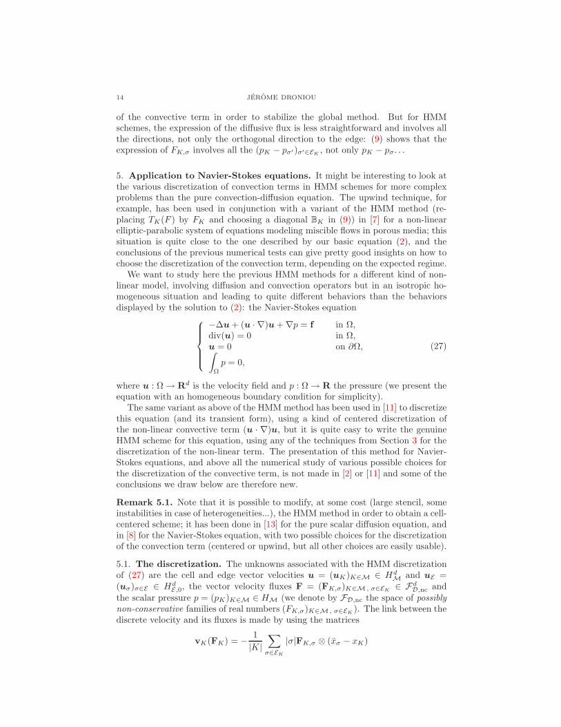
Grid 1 Grid 2

Figure 6. Grids used for the tests, on the lid-driven cavity case,of the HMM method for Navier-Stokes equations.

Equations (28)–(33) form the generic HMM discretization of (27), each schemeof the family being obtained by making specific choices of the stabilization matricesBK,i and of the numerical convection method, described by the flux function Fc.

5.2. Numerical results. It is quite straightforward to adapt the theoretical studymade in [11], using the computations from [2], to see that all the schemes obtainedby choosing any of the convective methods described above are convergent, underusual assumptions in the HMM setting on the mesh and stabilization matrices.We would like to present here some numerical results obtained by making differentchoices of Fc.

The test case we consider is the classical lid-driven cavity with Reynolds numberRe = 1000, using two kinds of grids (made of hexahedral cells), Grid 1 and Grid2, represented in Figure 6. Note that both grids are distorted, albeit in differentways (Grid 1 has many large cells which are distorted but its small cells are quiteregular, whereas this is basically the opposite for Grid 2). The solution to thenonlinear HMM schemes (28)–(33) is approximated using a relaxed Newton method,the linear system at each iteration being solved by the BiCGStab algorithm (withILU preconditioning).

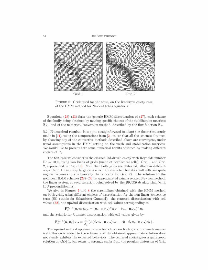
We give in Figures 7 and 8 the streamlines obtained with the HMM methodon both grids, using different choices of discretization for the non-linear convectiveterm (SG stands for Scharfetter-Gummel): the centered discretization with cellvalues (32), the upwind discretization with cell values corresponding to

Fuσ ·nc (u, uE)K,σ = (uσ · nK,σ)+uK − (uσ · nK,σ)−uL

and the Scharfetter-Gummel discretization with cell values given by

Fuσ·nc (u, uE)K,σ =

1

dσ

(A(dσuσ · nK,σ)uK − A(−dσuσ · nK,σ)uL) .

The upwind method appears to be a bad choice on both grids: too much numer-ical diffusion is added to the scheme, and the obtained approximate solution doesnot clearly exhibits the expected behaviors. The centered choice gives a quite goodsolution on Grid 1, but seems to strongly suffer from the peculiar distorsion of Grid

CONVECTION TERMS IN HMM METHODS 17

Centered (cell-based) Upwind (cell-based) SG (cell-based)

Figure 7. Comparison of different choices of discretization of thenon-linear convective term in Navier-Stokes equations, for the lid-driven cavity test case on Grid 1.

Centered (cell-based) Upwind (cell-based) SG (cell-based)

Figure 8. Comparison of different choices of discretization of thenon-linear convective term in Navier-Stokes equations, for the lid-driven cavity test case on Grid 2.

2 on which the solution it provides can be considered worst (albeit in an oppositeway) than the solution given by the upwind method. The solution provided by theScharfetter-Gummel discretization is not very good, but still better than the onegiven by the upwind scheme and, above all, seems more “stable” with respect to thedistorsions of the grids: on the contrary to the centered scheme, the solution of theScharfetter-Gummel technique on both grids are similar and more or less exhibitssome expected behavior of this test-case.

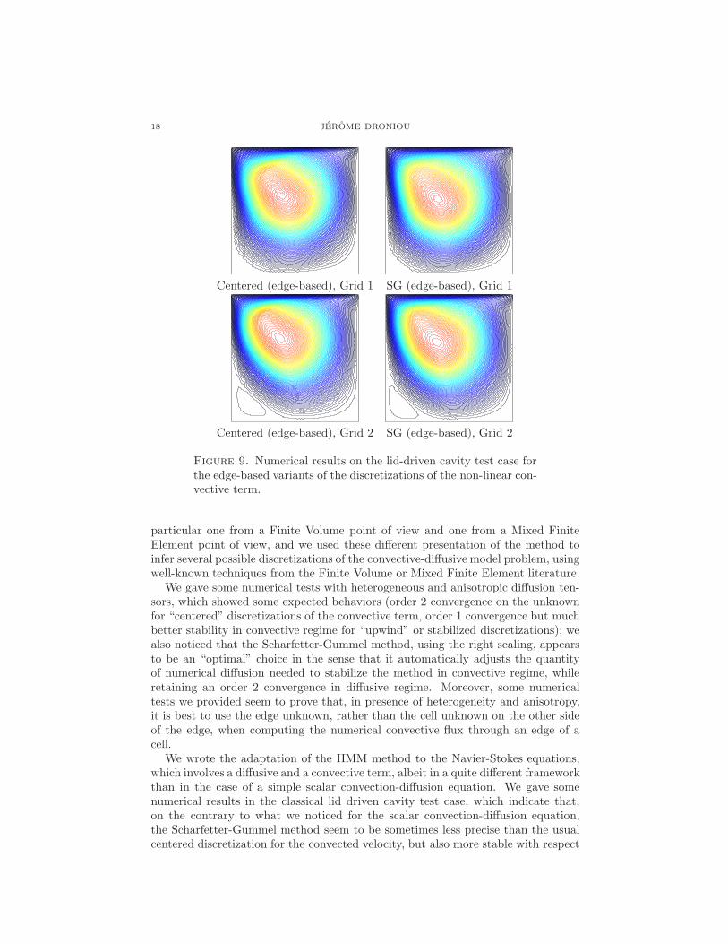
Figure 9 show some approximated solutions obtained using the edge-based vari-ants of the centered and Scharfetter-Gummel discretizations. These results, com-pared with the previous solutions obtained using the same methods with only thecell unknowns, seem to indicate that the use of the edge-based discretizations forthe nonlinear term in Navier-Stokes equations is not as interesting as for (2) in thecase of a discontinuous anistropic tensor (cf Section 4.2.1 and Figure 4).

6. Conclusion. We presented some discretizations of convection-diffusion equa-tions based on the HMM method, a family of schemes for diffusion operators whichgeneralizes the Hybrid Finite Volume, the Mimetic Finite Difference and the MixedFinite Volume schemes. The HMM method has several possible interpretations, in

18 JEROME DRONIOU

Centered (edge-based), Grid 1 SG (edge-based), Grid 1

Centered (edge-based), Grid 2 SG (edge-based), Grid 2

Figure 9. Numerical results on the lid-driven cavity test case forthe edge-based variants of the discretizations of the non-linear con-vective term.

particular one from a Finite Volume point of view and one from a Mixed FiniteElement point of view, and we used these different presentation of the method toinfer several possible discretizations of the convective-diffusive model problem, usingwell-known techniques from the Finite Volume or Mixed Finite Element literature.

We gave some numerical tests with heterogeneous and anisotropic diffusion ten-sors, which showed some expected behaviors (order 2 convergence on the unknownfor “centered” discretizations of the convective term, order 1 convergence but muchbetter stability in convective regime for “upwind” or stabilized discretizations); wealso noticed that the Scharfetter-Gummel method, using the right scaling, appearsto be an “optimal” choice in the sense that it automatically adjusts the quantityof numerical diffusion needed to stabilize the method in convective regime, whileretaining an order 2 convergence in diffusive regime. Moreover, some numericaltests we provided seem to prove that, in presence of heterogeneity and anisotropy,it is best to use the edge unknown, rather than the cell unknown on the other sideof the edge, when computing the numerical convective flux through an edge of acell.

We wrote the adaptation of the HMM method to the Navier-Stokes equations,which involves a diffusive and a convective term, albeit in a quite different frameworkthan in the case of a simple scalar convection-diffusion equation. We gave somenumerical results in the classical lid driven cavity test case, which indicate that,on the contrary to what we noticed for the scalar convection-diffusion equation,the Scharfetter-Gummel method seem to be sometimes less precise than the usualcentered discretization for the convected velocity, but also more stable with respect

CONVECTION TERMS IN HMM METHODS 19

to the grid distorsions. Similarly, the use of the edge unknown in this discretizationappears perhaps less useful than in the case of scalar heterogeneous anisotropicconvection-diffusion processes.

REFERENCES

[1] L. Beirao da Veiga and G. Manzini, A higher-order formulation of the mimetic finite difference

method, SIAM J. Sci. Comput., 31 (2008), 732–760.[2] L. Beirao da Veiga, J. Droniou and G. Manzini, A unified approach to handle convection

terms in mixed and hybrid finite volumes and mimetic finite difference methods, submittedfor publication.

[3] F. Brezzi, K. Lipnikov and M. Shashkov, Convergence of the mimetic finite difference method

for diffusion problems on polyhedral meshes, SIAM J. Numer. Anal., 43 (2005), 1872–1896.[4] F. Brezzi, K. Lipnikov and V. Simoncini, A family of mimetic finite difference methods on

polygonal and polyhedral meshes, Math. Models Methods Appl. Sci., 15 (2005), 1533–1551.[5] A. Cangiani, G. Manzini and A. Russo, Convergence analysis of a mimetic finite difference

method for general second-order elliptic problems, SIAM J. Numer. Anal., 47 (2009), 2612–2637.

[6] C. Chainais-Hillairet and J. Droniou, Finite volume schemes for non-coercive elliptic prob-

lems with Neumann boundary conditions, IMA Journal of Numerical Analysis, 2009. Doi:10.1093/imanum/drp009.

[7] C. Chainais-Hillairet and J. Droniou, Convergence analysis of a mixed finite volume scheme

for an elliptic-parabolic system modeling miscible fluid flows in porous media, SIAM J. Numer.Anal., 45 (2007), 2228–2258.

[8] E. Chenier, R. Eymard and R. Herbin, A collocated finite volume scheme to solve free con-

vection for general non-conforming grids, J. Comput. Phys., 228 (2009), 2296–2311.[9] J. Droniou, R. Eymard, T. Gallouet and R. Herbin, A unified approach to mimetic finite

difference, hybrid finite volume and mixed finite volume methods, Math. Models MethodsAppl. Sci. (M3AS), 20 (2010), 265–295.

[10] J. Droniou and R. Eymard, A mixed finite volume scheme for anisotropic diffusion problems

on any grid, Numer. Math., 105 (2006), 35–71.[11] J. Droniou and R. Eymard, Study of the mixed finite volume method for stokes and navier-

stokes equations, Numer. Meth. P. D. E., 25 (2009), 137–171.[12] R. Eymard, T. Gallouet and R. Herbin, Finite volume methods, In “P. G. Ciarlet and J.-

L. Lions, editors, Techniques of Scientific Computing, Part III,” Handbook of NumericalAnalysis, VII, pages 713–1020, North-Holland, Amsterdam, 2000.

[13] R. Eymard, T. Gallouet and R. Herbin, Discretisation of heterogeneous and

anisotropic diffusion problems on general non-conforming meshes, sushi: A

scheme using stabilisation and hybrid interfaces, to appear in IMAJNA, see alsohttp://hal.archives-ouvertes.fr/docs/00/21/18/28/PDF/suchi.pdf , 2008.

[14] R. Ewing, T. Russel and M. Wheeler, Simulation of miscible displacement using mixed meth-

ods and a modified method of characteristics, in Proceedings of the 7th SPE Symposium onReservoir Simulation, Dallas, TX, Paper SPE 12241, Society of Petroleum Engineers, 1983,71–81.

[15] D. T. F. Russell, Finite elements with characteristics for two-component incompressible mis-

cible displacement, in Proceedings of the 6th SPE Symposium on Reservoir Simulation, New

Orleans, Paper SPE 10500, Society of Petroleum Engineers, 1982, 123–135.[16] L. Scharfetter and H. K. Gummel, Large signal analysis of a silicon Read diode, IEEE Trans.

on Elec. Dev., 16 (1969), 64–77.[17] H. Wang, D. Liang, R. E. Ewing, S. L. Lyons and G. Qin, An approximation to miscible

fluid flows in porous media with point sources and sinks by an Eulerian-Lagrangian localized

adjoint method and mixed finite element methods, SIAM J. Sci. Comput., 22 (2000), 561–581.

Received January 2010; revised April 2010.

E-mail address: droniou@math.univ-montp2.fr