Reliable Vehicle State and Parameter

Estimation

by

Mohammad Pirani

A thesis

presented to the University of Waterloo

in fulfillment of the

thesis requirement for the degree of

Doctor of Philosophy

in

Mechanical and Mechatronics Engineering

Waterloo, Ontario, Canada, 2017

c© Mohammad Pirani 2017

Examining Committee Membership The following served on the Examining Com-

mittee for this thesis. The decision of the Examining Committee is by majority vote.

External Examiner NAME: Chun-Yi Su

TITlE: Professor, Mechanical Engineering

Supervisors NAME: Amir Khajepour

TITlE: Professor, Mechanical Engineering

NAME: Baris Fidan

TITlE: Associate Professor, Mechanical Engineering

Internal Member NAME: William M. Melek

TITlE: Professor, Mechanical Engineering

Internal Examiner NAME: Steven Waslander

TITlE: Associate Professor, Mechanical Engineering

Internal-external member NAME: David Wang

TITlE: Professor, Electrical and Computer Engineering

ii

Author’s Declaration

I hereby declare that I am the sole author of this thesis. This is a true copy of the thesis,

including any required final revisions, as accepted by my examiners.

I understand that my thesis may be made electronically available to the public.

iii

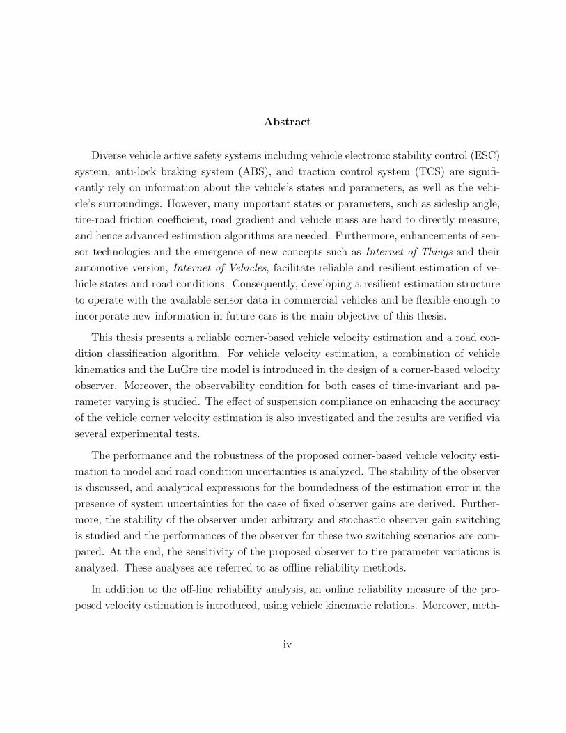
Abstract

Diverse vehicle active safety systems including vehicle electronic stability control (ESC)

system, anti-lock braking system (ABS), and traction control system (TCS) are signifi-

cantly rely on information about the vehicle’s states and parameters, as well as the vehi-

cle’s surroundings. However, many important states or parameters, such as sideslip angle,

tire-road friction coefficient, road gradient and vehicle mass are hard to directly measure,

and hence advanced estimation algorithms are needed. Furthermore, enhancements of sen-

sor technologies and the emergence of new concepts such as Internet of Things and their

automotive version, Internet of Vehicles, facilitate reliable and resilient estimation of ve-

hicle states and road conditions. Consequently, developing a resilient estimation structure

to operate with the available sensor data in commercial vehicles and be flexible enough to

incorporate new information in future cars is the main objective of this thesis.

This thesis presents a reliable corner-based vehicle velocity estimation and a road con-

dition classification algorithm. For vehicle velocity estimation, a combination of vehicle

kinematics and the LuGre tire model is introduced in the design of a corner-based velocity

observer. Moreover, the observability condition for both cases of time-invariant and pa-

rameter varying is studied. The effect of suspension compliance on enhancing the accuracy

of the vehicle corner velocity estimation is also investigated and the results are verified via

several experimental tests.

The performance and the robustness of the proposed corner-based vehicle velocity esti-

mation to model and road condition uncertainties is analyzed. The stability of the observer

is discussed, and analytical expressions for the boundedness of the estimation error in the

presence of system uncertainties for the case of fixed observer gains are derived. Further-

more, the stability of the observer under arbitrary and stochastic observer gain switching

is studied and the performances of the observer for these two switching scenarios are com-

pared. At the end, the sensitivity of the proposed observer to tire parameter variations is

analyzed. These analyses are referred to as offline reliability methods.

In addition to the off-line reliability analysis, an online reliability measure of the pro-

posed velocity estimation is introduced, using vehicle kinematic relations. Moreover, meth-

iv

ods to distinguish measurement faults from estimation faults are presented. Several exper-

imental results are provided to verify the approach.

An algorithm for identifying (classifying) road friction is proposed in this thesis. The

analytical foundation of this algorithm, which is based on vehicle response to lateral excita-

tion, is introduced and its performance is discussed and compared to previous approaches.

The sensitivity of this algorithm to vehicle/tire parameter variations is also studied. At

the end, various experimental results consisting of several maneuvers on different road

conditions are presented to verify the performance of the algorithm.

v

Acknowledgements

Foremost, I would like to express my many thanks to Prof. Amir Khajepour and Prof.

Baris Fidan, for their support, encouragement, and supervision of the research presented

in this thesis.

I also would like to acknowledge the financial support of Automotive Partnership

Canada, Ontario Research Fund and General Motors. I extend my appreciation to Prof.

Chun-Yi Su, Prof. Steven Waslander, Prof. William Melek and Prof. David Wang for

their role as readers of the thesis.

I want to express my appreciation to Prof. Shreyas Sundaram for the interactions and

scientific collaborations that we have had over the years which inspired me in my research.

My whole experience would not have been as rewarding without the help of my colleague

Ehsan Hashemi. I am also grateful to Ebrahim Moradi Shahrivar, Mohsen Raeis-Zadeh,

Mehdi Jalalmaab and all my friend in Waterloo and Toronto for all the hangouts, laughters

and travels that we have shared.

I am deeply grateful to my sister Parisa, her husband Abouzar and their lovely daughter

Hannah. Most importantly, none of this would have been possible without the patience,

love and support of my parents, Fereidoon Pirani and Mahboobeh Heydari, whom I cor-

dially dedicate the honor of all my current and future achievements to.

vi

Table of Contents

List of Figures x

1 Introduction 3

1.1 Motivation . . . . . . . . . . . . . . . . . . . . . . . . . . . . . . . . . . . . 3

1.2 Objectives . . . . . . . . . . . . . . . . . . . . . . . . . . . . . . . . . . . . 7

1.3 Thesis Outline . . . . . . . . . . . . . . . . . . . . . . . . . . . . . . . . . . 8

2 Background and Literature Review 10

2.1 Vehicle States and Road Condition Estimation . . . . . . . . . . . . . . . . 10

2.2 Literature Review and Background on Vehicle Tire Modeling . . . . . . . . 13

2.2.1 Static Tire Model . . . . . . . . . . . . . . . . . . . . . . . . . . . . 15

2.2.2 Dynamic Tire Model . . . . . . . . . . . . . . . . . . . . . . . . . . 15

2.2.3 LuGre Tire Model . . . . . . . . . . . . . . . . . . . . . . . . . . . 16

2.3 Vehicle Lateral Dynamics . . . . . . . . . . . . . . . . . . . . . . . . . . . 17

2.3.1 Linear Lateral Dynamics Model . . . . . . . . . . . . . . . . . . . . 17

2.3.2 Nonlinear Lateral Dynamics Model . . . . . . . . . . . . . . . . . . 19

2.4 Estimation Reliability . . . . . . . . . . . . . . . . . . . . . . . . . . . . . 21

2.4.1 Probabilistic methods in reliable estimator design . . . . . . . . . . 23

2.5 Summary . . . . . . . . . . . . . . . . . . . . . . . . . . . . . . . . . . . . 25

vii

3 Vehicle Corner Velocity Estimation 26

3.1 Longitudinal Velocity Estimation . . . . . . . . . . . . . . . . . . . . . . . 26

3.2 Lateral Velocity Estimation . . . . . . . . . . . . . . . . . . . . . . . . . . 29

3.3 Model improvement by Inclusion of Suspension Compliance . . . . . . . . . 31

3.3.1 Suspension Model . . . . . . . . . . . . . . . . . . . . . . . . . . . . 31

3.4 Experimental Validation . . . . . . . . . . . . . . . . . . . . . . . . . . . . 34

3.4.1 Experimental Setup . . . . . . . . . . . . . . . . . . . . . . . . . . . 36

3.4.2 Maneuvers with longitudinal excitations . . . . . . . . . . . . . . . 37

3.4.3 Maneuvers with lateral and combined lateral/longitudinal excitations 40

3.5 Summary . . . . . . . . . . . . . . . . . . . . . . . . . . . . . . . . . . . . 44

4 Reliability of the Vehicle Corner Velocity Estimation 46

4.1 Estimator’s Stability, Robustness and Sensitivity Analysis . . . . . . . . . 47

4.1.1 Stability and H∞ Performance . . . . . . . . . . . . . . . . . . . . . 47

4.1.2 Sensitivity of the Stability Margin and H∞ Performance to Tire Pa-

rameters . . . . . . . . . . . . . . . . . . . . . . . . . . . . . . . . . 52

4.2 Stability of the Estimator Under Gain Switching . . . . . . . . . . . . . . . 53

4.2.1 Stability of the observer under arbitrarily switching gains . . . . . . 55

4.2.2 Stability of the observer under stochastically switching gains . . . . 55

4.3 Reliable Velocity Estimator in the Presence of Faulty Measurements . . . . 57

4.4 Summary . . . . . . . . . . . . . . . . . . . . . . . . . . . . . . . . . . . . 60

5 On-line Reliability Measures 61

5.1 Procedure . . . . . . . . . . . . . . . . . . . . . . . . . . . . . . . . . . . . 62

5.1.1 Distinguishing Measurement Faults from Estimation Faults . . . . . 63

viii

5.2 Applying Reliability Indices to Modify the Estimated Velocities . . . . . . 66

5.2.1 Some network definitions . . . . . . . . . . . . . . . . . . . . . . . . 66

5.2.2 Opinion Dynamics for Reliable Vehicle Estimation . . . . . . . . . . 66

5.3 Experimental Results . . . . . . . . . . . . . . . . . . . . . . . . . . . . . . 69

5.3.1 Acceleration-Deceleration on Dry Road . . . . . . . . . . . . . . . . 69

5.3.2 Steering on Dry Road . . . . . . . . . . . . . . . . . . . . . . . . . 71

5.3.3 Steering on Basalt Tiles . . . . . . . . . . . . . . . . . . . . . . . . 72

5.3.4 Steering on a Wet Road . . . . . . . . . . . . . . . . . . . . . . . . 74

5.4 Summary . . . . . . . . . . . . . . . . . . . . . . . . . . . . . . . . . . . . 75

6 Road Condition Identification 76

6.1 Vehicle Response-Based Road Condition Classification . . . . . . . . . . . 78

6.1.1 Linear Tire Model Case . . . . . . . . . . . . . . . . . . . . . . . . 78

6.1.2 Nonlinear Tire Model Case . . . . . . . . . . . . . . . . . . . . . . . 81

6.2 Experimental Results . . . . . . . . . . . . . . . . . . . . . . . . . . . . . . 82

6.2.1 Slaloms on Dry (Using Linear Tire Model) . . . . . . . . . . . . . . 82

6.2.2 Maneuvers with Nonlinear Excitations . . . . . . . . . . . . . . . . 84

6.3 Summary . . . . . . . . . . . . . . . . . . . . . . . . . . . . . . . . . . . . 86

7 Conclusion and Future Works 88

7.1 Summary and Conclusions . . . . . . . . . . . . . . . . . . . . . . . . . . . 88

7.2 Future Work . . . . . . . . . . . . . . . . . . . . . . . . . . . . . . . . . . . 90

7.2.1 Improving Estimation for a Single Vehicle . . . . . . . . . . . . . . 90

7.2.2 Application of Vehicle Networks to Vehicle State Estimation . . . . 92

References 94

ix

List of Figures

1.1 Vehicle state estimation in the overall vehicle control scheme. . . . . . . . . 4

1.2 The objectives of the thesis in a glimpse. . . . . . . . . . . . . . . . . . . . 8

2.1 (a) The nonlinear tire force-slip relation for longitudinal motion and various

road conditions. (b) Tire geometric characteristics. . . . . . . . . . . . . . 15

2.2 The curve obtained from the Magic formula [1]. . . . . . . . . . . . . . . . 16

2.3 The tire forces and side slip angles in each track. . . . . . . . . . . . . . . . 18

2.4 Reliable estimator or controller design. . . . . . . . . . . . . . . . . . . . . 24

3.1 The effect of the suspension compliance on the vehicle corner velocities are

schematically represented by spring and dampers. . . . . . . . . . . . . . . 32

3.2 Assessment of the effect of the suspension compliance via tire model. . . . 33

3.3 Overall vehicle velocity estimation structure with SC. . . . . . . . . . . . . 35

3.4 Experimental setup for vehicle Estimation. . . . . . . . . . . . . . . . . . . 36

3.5 Test vehicles used in experimental verifications. . . . . . . . . . . . . . . . 37

3.6 Effect of the SC on corner longitudinal velocity estimation in acceleration

and brake, AWD. . . . . . . . . . . . . . . . . . . . . . . . . . . . . . . . . 39

3.7 SC verification with longitudinal forces in acceleration and brake, AWD. . 39

3.8 Launch on split-µ, ice/dry, and AWD. . . . . . . . . . . . . . . . . . . . . . 40

x

3.9 SC verification with longitudinal forces, split-µ and AWD. . . . . . . . . . 41

3.10 Acceleration in turn on a dry road, AWD. . . . . . . . . . . . . . . . . . . 42

3.11 SC verification with longitudinal forces, acceleration in turn and AWD. . . 42

3.12 Lateral velocity estimation for acceleration in turn on a dry road. . . . . . 43

3.13 SC verification with longitudinal forces, acceleration in turn, and AWD. . . 43

3.14 Lane change and steering on a snow road. . . . . . . . . . . . . . . . . . . 44

3.15 Lateral velocity estimates for a lane change (LC) on a snow road. . . . . . 45

4.1 System H∞ norm for longitudinal and lateral estimators. . . . . . . . . . . 50

4.2 Time-varying observer gains for the longitudinal estimator. . . . . . . . . . 51

4.3 Time-varying observer gains for the lateral estimator. . . . . . . . . . . . . 52

4.4 Sensitivity of SM of (3.9) and (3.15). . . . . . . . . . . . . . . . . . . . . . 53

4.5 Sensitivity of SM of (3.9) and (3.15) to σ1q. . . . . . . . . . . . . . . . . . 53

4.6 Sensitivity of H∞ norm of (3.9) and (3.15). . . . . . . . . . . . . . . . . . . 54

4.7 Tire forces (which are fed into the estimators) can be faulty. . . . . . . . . 54

4.8 Spectral radius ρ with respect to γ. . . . . . . . . . . . . . . . . . . . . . . 57

4.9 Critical probabilities for the velocity observers. . . . . . . . . . . . . . . . . 59

4.10 Spectral radius vs. failure probability for various ω. . . . . . . . . . . . . . 59

5.1 On-line reliability measure unit. . . . . . . . . . . . . . . . . . . . . . . . . 62

5.2 Overall scheme of the online reliability analysis. . . . . . . . . . . . . . . . 63

5.3 Detecting measurement fault. . . . . . . . . . . . . . . . . . . . . . . . . . 64

5.4 The method of bank of reliability indices. . . . . . . . . . . . . . . . . . . . 65

5.5 Corner opinions and their confidence level. . . . . . . . . . . . . . . . . . . 67

5.6 Enhancing the reliability of estimated corner velocities via opinion dynamics. 68

xi

5.7 Vehicle motion characteristics for an acceleration-deceleration maneuver. . 70

5.8 The reliability index of an acceleration-deceleration maneuver. . . . . . . . 70

5.9 Vehicle motion characteristics for a steering maneuver on a dry road. . . . 71

5.10 The reliability index of a steering maneuver on a dry road. . . . . . . . . . 72

5.11 Vehicle motion characteristics for a steering maneuver on Basalt. . . . . . . 73

5.12 The reliability index of a steering maneuver on a Basalt. . . . . . . . . . . 73

5.13 Vehicle motion characteristics for a steering maneuver on a wet road. . . . 74

5.14 The reliability index of a steering maneuver on a wet road. . . . . . . . . . 75

6.1 Sensitivity of the linear region of the tire model. . . . . . . . . . . . . . . . 77

6.2 Road condition identification procedure. . . . . . . . . . . . . . . . . . . . 82

6.3 Vehicle accelerations (left), and road identification residual Rr(t) (right) for

a harsh steering on a dry road. . . . . . . . . . . . . . . . . . . . . . . . . . 83

6.4 Vehicle accelerations (left), and road identification residual Rr(t) (right) for

a mild steering on a dry road. . . . . . . . . . . . . . . . . . . . . . . . . . 83

6.5 Yaw rate residual Rr(t) (top), general residual R(t) (middle) and vehicle

accelerations (bottom) for a Step steering on a dry road. . . . . . . . . . . 85

6.6 Yaw rate residual Rr(t) (top), general residual R(t) (middle) and vehicle

accelerations (bottom) for a steering on snow. . . . . . . . . . . . . . . . . 86

6.7 Yaw rate residual Rr(t) (top), general residual R(t) (middle) and vehicle

accelerations (bottom) for several turns on dry and wet roads. . . . . . . . 87

7.1 Reciprocity between vehicle velocity estimation and road condition identifi-

cation. . . . . . . . . . . . . . . . . . . . . . . . . . . . . . . . . . . . . . . 91

7.2 Distributed vehicle velocity fault diagnostics procedure. . . . . . . . . . . . 93

xii

Nomenclature

1

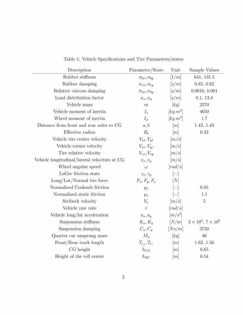
Table 1: Vehicle Specifications and Tire Parameters/states

Description Parameter/State Unit Sample Values

Rubber stiffness σ0x, σ0y [1/m] 641, 131.5

Rubber damping σ1x, σ1y [s/m] 0.85, 0.82

Relative viscous damping σ2x, σ2y [s/m] 0.0016, 0.001

Load distribution factor κx, κy [s/m] 8.1, 13.4

Vehicle mass m [kg] 2270

Vehicle moment of inertia Iz [kg.m2] 4650

Wheel moment of inertia Iw [kg.m2] 1.7

Distance from front and rear axles to CG a, b [m] 1.42, 1.43

Effective radius Re [m] 0.33

Vehicle tire center velocity Vxt, Vyt [m/s]

Vehicle corner velocity Vxc, Vyc [m/s]

Tire relative velocity Vrx, Vry [m/s]

Vehicle longitudinal/lateral velocities at CG vx, vy [m/s]

Wheel angular speed ω [rad/s]

LuGre friction state zx, zy [−]

Long/Lat/Normal tire force Fx, Fy, Fx [N ]

Normalized Coulomb friction µc [−] 0.85

Normalized static friction µs [−] 1.1

Stribeck velocity Vs [m/s] 5

Vehicle yaw rate r [rad/s]

Vehicle long/lat acceleration ax, ay [m/s2]

Suspension stiffness Kx, Ky [N/m] 3× 105, 7× 105

Suspension damping Cx, Cy [Ns/m] 3730

Quarter car unsprung mass Mu [kg] 46

Front/Rear track length Trf , Trr [m] 1.62, 1.56

CG height hCG [m] 0.65

Height of the roll center hRC [m] 0.54

2

Chapter 1

Introduction

1.1 Motivation

Great advancements in vehicular technologies have resulted in increasingly sophisticated

vehicles in recent years. While a vehicle’s economic performance and ride comfort are de-

veloped via optimizing the energy management system and advanced suspension system,

vehicle active safety systems are critical to the driving safety of vehicles and are becoming

more and more important. The annual report announced by Canada Ministry of Trans-

portation on traffic collisions and crash statistics echoes the necessity of automotive safety

and reveals the importance of enhancing active safety based on the todays multifarious ur-

ban requirements. Diverse representations of vehicle active safety system include (but are

not limited to): vehicle electronic stability control (ESC) system, anti-lock braking system

(ABS), and traction control system (TCS). It is commonly recognized that the operation

of active safety systems significantly rely on information about the vehicle’s states and

parameters as well as the vehicle’s surroundings. For instance, the control strategies men-

tioned above are considering the vehicle’s time-varying longitudinal and lateral velocities.

However, many of the important states or parameters, such as sideslip angle, tire-road fric-

tion coefficient, road gradient, and vehicle mass, are hard to directly measure, so advanced

estimation algorithms have to be developed. Hence, having a cost efficient vehicle state

and road condition estimation is a necessity for active safety systems in current commercial

3

vehicles, and the ongoing research in this field highlights this importance. Furthermore,

enhancements of sensor technologies and the emergence of new concepts such as Internet

of Things and their automotive version, Internet of Vehicles, facilitate reliable and resilient

estimation of vehicle states and road condition. Consequently, developing a resilient esti-

mation structure to operate with the available sensor data in commercial vehicles and be

flexible to incorporating new information in future cars is a preeminent objective. Two

major practical issues that have dominated the vehicle state/parameter estimation field are

vehicle velocity estimation, in both longitudinal and lateral directions, and road condition

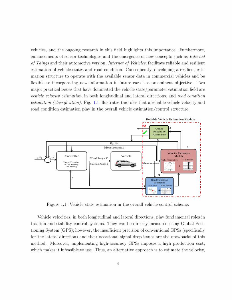
estimation (classification). Fig. 1.1 illustrates the roles that a reliable vehicle velocity and

road condition estimation play in the overall vehicle estimation/control structure.

𝒆

𝑣 𝑥, 𝑣 𝑦

Vehicle

Measurements

Velocity Estimation

Module

Tire Model

+

Veh. Kinematics Wheel Torque 𝑇

Steering Angle 𝛿

Road Condition

Estimation

Tire Model

+

Veh. Dyn

Controller

Torque Vectoring

Active Steering

Diff Braking

𝜽

𝒓𝒅, 𝝀𝒅

Online

Reliability

Assessment

1

2

3

Measurements

Reliable Vehicle Estimation Module

Figure 1.1: Vehicle state estimation in the overall vehicle control scheme.

Vehicle velocities, in both longitudinal and lateral directions, play fundamental roles in

traction and stability control systems. They can be directly measured using Global Posi-

tioning System (GPS); however, the insufficient precision of conventional GPSs (specifically

for the lateral direction) and their occasional signal drop issues are the drawbacks of this

method. Moreover, implementing high-accuracy GPSs imposes a high production cost,

which makes it infeasible to use. Thus, an alternative approach is to estimate the velocity,

4

based on available sensor data instead of direct measurement. To this end, the prominence

of having a reliable velocity estimation that is resilient to the road condition and vehicle

parameter uncertainties, has been amplified in recent research in automotive control and

autonomous driving systems. There has been much effort in utilizing the latest theoretical

results as well as overcoming technical obstacles to estimate vehicle longitudinal and lateral

velocities via using the few available sensor measurements embedded in conventional cars.

From a theoretical perspective, the fact is that a more accurate vehicle model results in a

more precise vehicle velocity estimation. The imprecision in the vehicle dynamics can be

rooted in an inaccurate tire model or the omission of some additional dynamics, such as the

effect of the suspension compliance on the wheel speed. Moreover, the effect of the driver’s

actions is another unmodeled dynamics that should be taken into account as well. Hence,

in order to come up with a reliable vehicle velocity estimation, detailed vehicle dynamics

obtained from an accurate tire model with a known road condition are needed.

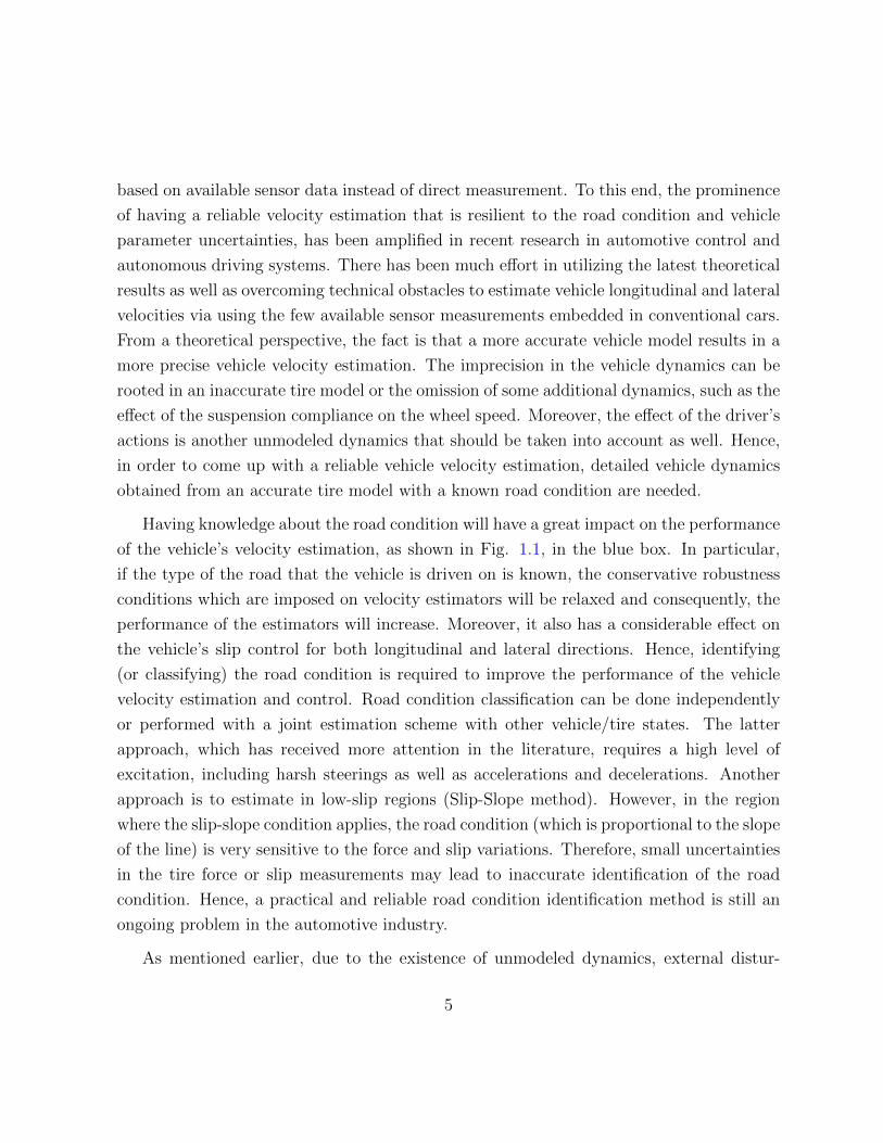
Having knowledge about the road condition will have a great impact on the performance

of the vehicle’s velocity estimation, as shown in Fig. 1.1, in the blue box. In particular,

if the type of the road that the vehicle is driven on is known, the conservative robustness

conditions which are imposed on velocity estimators will be relaxed and consequently, the

performance of the estimators will increase. Moreover, it also has a considerable effect on

the vehicle’s slip control for both longitudinal and lateral directions. Hence, identifying

(or classifying) the road condition is required to improve the performance of the vehicle

velocity estimation and control. Road condition classification can be done independently

or performed with a joint estimation scheme with other vehicle/tire states. The latter

approach, which has received more attention in the literature, requires a high level of

excitation, including harsh steerings as well as accelerations and decelerations. Another

approach is to estimate in low-slip regions (Slip-Slope method). However, in the region

where the slip-slope condition applies, the road condition (which is proportional to the slope

of the line) is very sensitive to the force and slip variations. Therefore, small uncertainties

in the tire force or slip measurements may lead to inaccurate identification of the road

condition. Hence, a practical and reliable road condition identification method is still an

ongoing problem in the automotive industry.

As mentioned earlier, due to the existence of unmodeled dynamics, external distur-

5

bances and occasional measurement faults, failures in estimation algorithms during real

time implementation are unavoidable. To address this issue, it is imperative to design a

reliability monitoring module, beside vehicle velocity estimation, as shown in Fig. 1.1, in

the green box. Two general approaches can address the reliability of a vehicle velocity

estimation:

1. Real time (on-line) approach: In this method, during the estimator operation, the

estimated velocity is concurrently translated into parameters that can be measured

directly with a desirable accuracy. Finally, by comparing the results, a level of relia-

bility is determined. A simple example of this method is to translate the estimated

velocity (in each direction) to the measured acceleration in the corresponding direc-

tion, measured from the IMU, and compare them to find a possible failure in the

estimation.

2. Offline methods: These methods provide the fundamental limitations that a vehicle

velocity estimator faces in terms of its performance and robustness to inaccuracies

of parameters and input data such as road conditions and sensor measurements.

To yield this, one can utilize robustness and stability theorems available in systems

and control literature to come up with analytical descriptions of the reliability of

the estimator. Since such analyses show the characteristics of the designed velocity

estimator and can be determined offline, they are referred to as offline methods.

The advantage of a real time approach is that it can provide information regarding the reli-

ability of the estimator in a concurrent manner. However, the advantage of off-line methods

is to propose concrete milestones (in terms of vehicle characteristics and road condition)

that should be met in order to reach to a desirable estimation. As mentioned, one of the

main sources of unreliability of the vehicle velocity estimation is the uncertainty in road

condition. Due to this fact, reliable velocity estimation and road condition identification

always coexist in such studies.

6

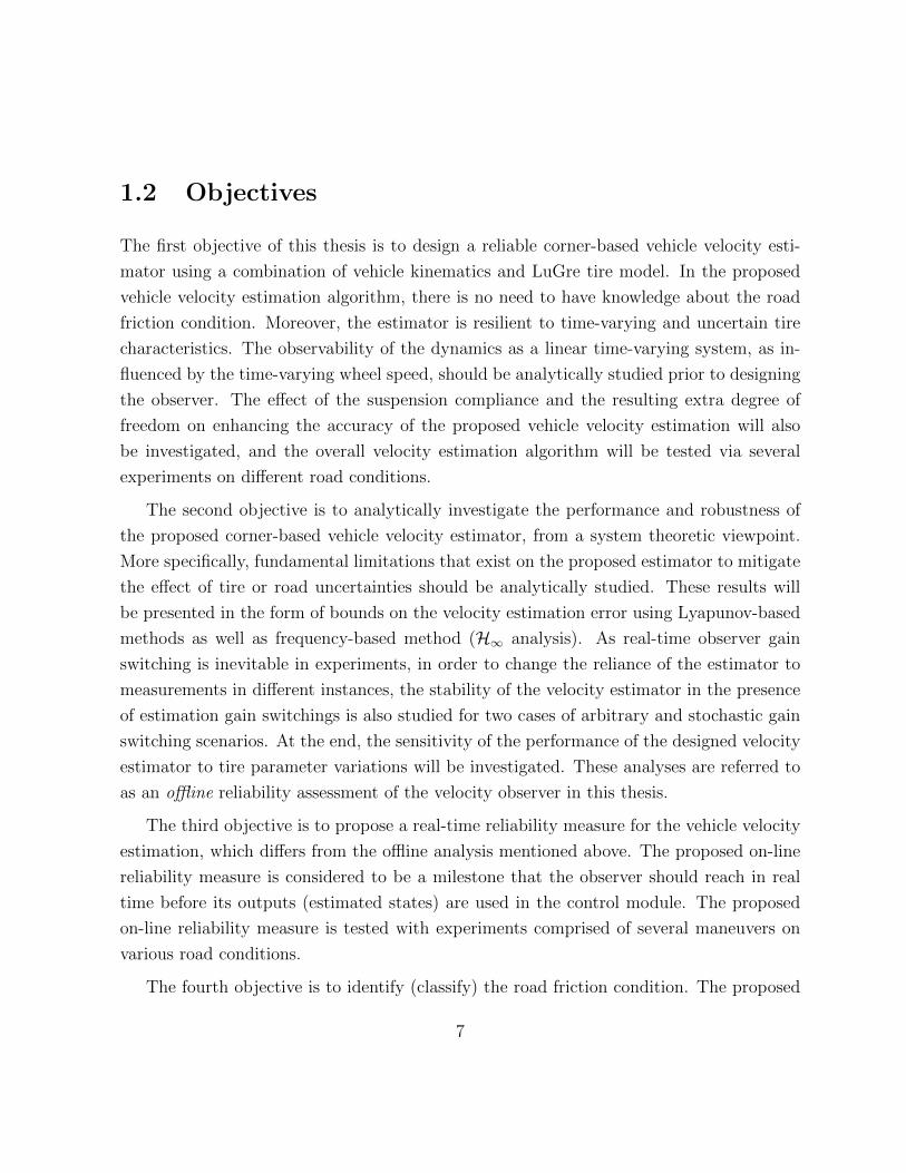
1.2 Objectives

The first objective of this thesis is to design a reliable corner-based vehicle velocity esti-

mator using a combination of vehicle kinematics and LuGre tire model. In the proposed

vehicle velocity estimation algorithm, there is no need to have knowledge about the road

friction condition. Moreover, the estimator is resilient to time-varying and uncertain tire

characteristics. The observability of the dynamics as a linear time-varying system, as in-

fluenced by the time-varying wheel speed, should be analytically studied prior to designing

the observer. The effect of the suspension compliance and the resulting extra degree of

freedom on enhancing the accuracy of the proposed vehicle velocity estimation will also

be investigated, and the overall velocity estimation algorithm will be tested via several

experiments on different road conditions.

The second objective is to analytically investigate the performance and robustness of

the proposed corner-based vehicle velocity estimator, from a system theoretic viewpoint.

More specifically, fundamental limitations that exist on the proposed estimator to mitigate

the effect of tire or road uncertainties should be analytically studied. These results will

be presented in the form of bounds on the velocity estimation error using Lyapunov-based

methods as well as frequency-based method (H∞ analysis). As real-time observer gain

switching is inevitable in experiments, in order to change the reliance of the estimator to

measurements in different instances, the stability of the velocity estimator in the presence

of estimation gain switchings is also studied for two cases of arbitrary and stochastic gain

switching scenarios. At the end, the sensitivity of the performance of the designed velocity

estimator to tire parameter variations will be investigated. These analyses are referred to

as an offline reliability assessment of the velocity observer in this thesis.

The third objective is to propose a real-time reliability measure for the vehicle velocity

estimation, which differs from the offline analysis mentioned above. The proposed on-line

reliability measure is considered to be a milestone that the observer should reach in real

time before its outputs (estimated states) are used in the control module. The proposed

on-line reliability measure is tested with experiments comprised of several maneuvers on

various road conditions.

The fourth objective is to identify (classify) the road friction condition. The proposed

7

road friction identification algorithm is based on vehicle responses, vehicle lateral dynamics

and appropriate tire models. This algorithm can take advantage of receiving information

from the road-independent velocity estimation module to enhance its accuracy and per-

formance. The performance of this algorithm will be verified via various experiments on

different road conditions and for different maneuvers. The resilience of the proposed algo-

rithm to tire and vehicle parameter uncertainties will be also be discussed.

The objectives of this thesis and the connections between topics discussed above are

shown in Fig. 1.2.

Corner-Based Velocity Estimator Design

+

Model Improvement with Suspension Compliance

Vehicle Velocity Estimation

Chapter 3

Road Condition Identification

Algorithm + Experiments

Chapter 6

𝑣 𝑦, 𝑣 𝑥

Estimation Reliability Analysis

Off-line Reliability Measure

Stability, robustness and

sensitivity analysis

Chapter

4

On-line Reliability Measure

Algorithm + Experiments

Chapter

5

𝑣 𝑦, 𝑣 𝑥

Figure 1.2: The objectives of the thesis in a glimpse.

1.3 Thesis Outline

In the second chapter of this thesis, a literature review on vehicle state and parameter esti-

mation, specifically vehicle velocity and road condition estimation, is presented. Moreover,

an overview of studies done in reliable system and controller (estimator) design, for deter-

8

ministic and stochastic systems, are discussed. Furthermore, a brief background on vehicle

tire model as well as vehicle lateral dynamics (known as bicycle model) is introduced.

In the third chapter, the vehicle corner-based velocity estimator is proposed. More

specifically, the combination of vehicle kinematics and the LuGre tire model is introduced

in the design of the base dynamics for a corner-based velocity observer of the vehicle. More-

over, the observability condition for both cases of time-invariant and parameter varying

is studied. At the end, the effect of suspension compliance on enhancing the accuracy of

the vehicle corner velocity estimation is also investigated and the results are verified via

several experimental tests.

In the fourth chapter, the performance and the robustness of the proposed corner-based

vehicle velocity estimation to model and road condition uncertainties is analyzed. The

stability of the observer is discussed, and analytical expressions for the boundedness of the

estimation error in the presence of system uncertainties for the case of fixed observer gains

are derived. Furthermore, the stability of the observer under arbitrary and stochastic

observer gain switching is studied and the performances of the observer for these two

switching scenarios are compared. At the end, the sensitivity of the proposed observer to

tire parameter variations is analyzed.

Chapter five presents an online reliability measure of the proposed velocity estimation,

using vehicle kinematic relations. Moreover, methods to distinguish measurement faults

from estimation faults are presented. Several experimental results are also provided to

verify the approach.

Chapter six pertains to proposing an algorithm for the road condition identification.

The analytical foundation of this algorithm, which is based on vehicle response to lat-

eral excitation, is introduced and its performance is discussed and compared to previous

approaches. The sensitivity of this algorithm to vehicle/tire parameter variations is also

studied. At the end, various experimental results consisting of several maneuvers on dif-

ferent road conditions are presented to verify the performance of the algorithm.

In chapter seven, the conclusions and the contributions of this thesis are presented.

Moreover, some possible future avenues for further research are mentioned.

9

Chapter 2

Background and Literature Review

In this chapter, a comprehensive literature review on the vehicle states, road condition

estimation, and reliability of the estimators is presented. Moreover, a brief background on

the vehicle tire model as well as vehicle lateral dynamics is presented, both of which will

be used later in the thesis.

2.1 Vehicle States and Road Condition Estimation

Advanced vehicle stability control and active safety systems require dependable vehicle

states, which may not be accessible by measurements so they should be estimated. Two

major practical issues that have dominated the vehicle state estimation field are velocity

and tire force estimations that are robust to road friction changes.

Tire forces are one of the main vehicle states that should be estimated and they have

a great degree of influence in corner based vehicle velocity estimation. Tire forces can

be measured at each corner with sensors mounted on the wheel hub, but their significant

cost, required space, and calibration and maintenance make them completely unfeasible

for mass production vehicles. Provided that the tire force calculation needs road friction,

even accurate slip ratio/angle information from the GPS will not engender forces at each

corner. Estimation of longitudinal and lateral forces independent from the road condition

10

may be classified on the basis of wheel dynamics into the nonlinear and sliding mode

observers [2–4], Kalman-based estimation [5–7], and unknown input observers [8–10]. A

force estimation method based on the steering torque measurement is introduced in [11],

which requires additional measurements.

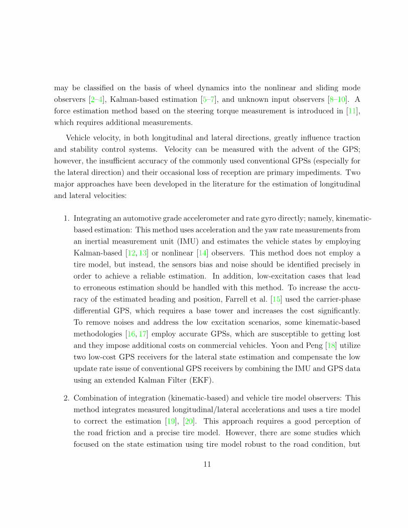
Vehicle velocity, in both longitudinal and lateral directions, greatly influence traction

and stability control systems. Velocity can be measured with the advent of the GPS;

however, the insufficient accuracy of the commonly used conventional GPSs (especially for

the lateral direction) and their occasional loss of reception are primary impediments. Two

major approaches have been developed in the literature for the estimation of longitudinal

and lateral velocities:

1. Integrating an automotive grade accelerometer and rate gyro directly; namely, kinematic-

based estimation: This method uses acceleration and the yaw rate measurements from

an inertial measurement unit (IMU) and estimates the vehicle states by employing

Kalman-based [12, 13] or nonlinear [14] observers. This method does not employ a

tire model, but instead, the sensors bias and noise should be identified precisely in

order to achieve a reliable estimation. In addition, low-excitation cases that lead

to erroneous estimation should be handled with this method. To increase the accu-

racy of the estimated heading and position, Farrell et al. [15] used the carrier-phase

differential GPS, which requires a base tower and increases the cost significantly.

To remove noises and address the low excitation scenarios, some kinematic-based

methodologies [16, 17] employ accurate GPSs, which are susceptible to getting lost

and they impose additional costs on commercial vehicles. Yoon and Peng [18] utilize

two low-cost GPS receivers for the lateral state estimation and compensate the low

update rate issue of conventional GPS receivers by combining the IMU and GPS data

using an extended Kalman Filter (EKF).

2. Combination of integration (kinematic-based) and vehicle tire model observers: This

method integrates measured longitudinal/lateral accelerations and uses a tire model

to correct the estimation [19], [20]. This approach requires a good perception of

the road friction and a precise tire model. However, there are some studies which

focused on the state estimation using tire model robust to the road condition, but

11

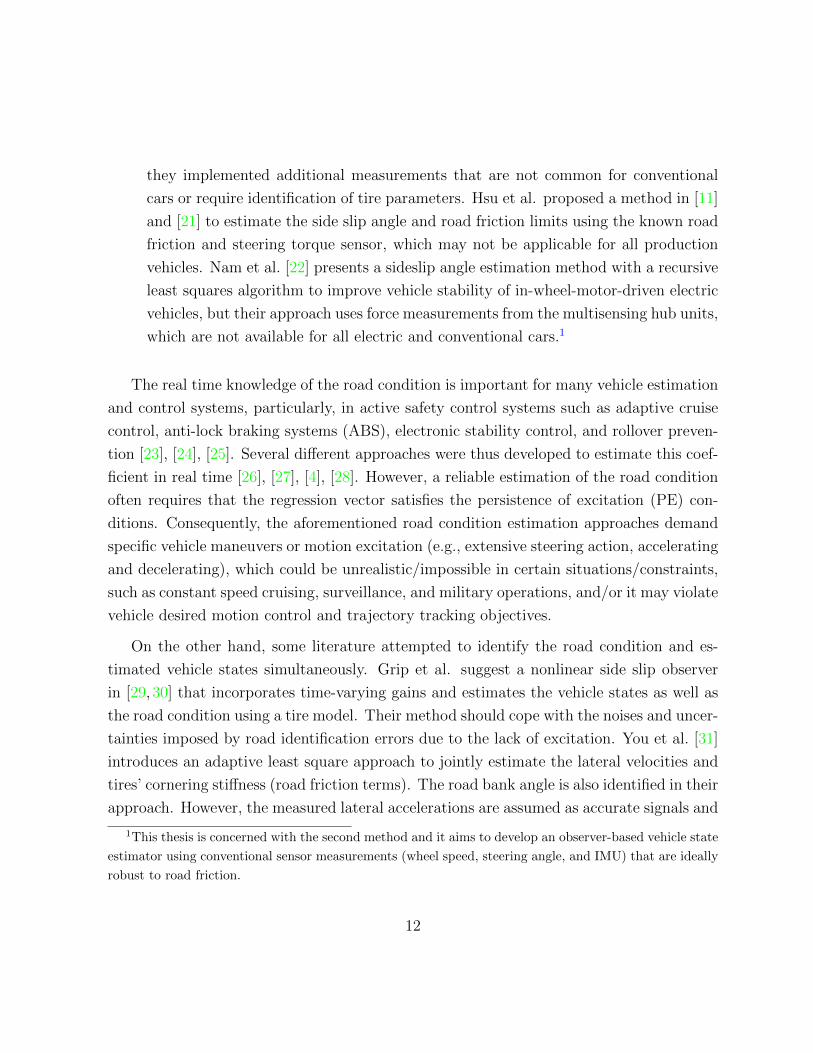
they implemented additional measurements that are not common for conventional

cars or require identification of tire parameters. Hsu et al. proposed a method in [11]

and [21] to estimate the side slip angle and road friction limits using the known road

friction and steering torque sensor, which may not be applicable for all production

vehicles. Nam et al. [22] presents a sideslip angle estimation method with a recursive

least squares algorithm to improve vehicle stability of in-wheel-motor-driven electric

vehicles, but their approach uses force measurements from the multisensing hub units,

which are not available for all electric and conventional cars.1

The real time knowledge of the road condition is important for many vehicle estimation

and control systems, particularly, in active safety control systems such as adaptive cruise

control, anti-lock braking systems (ABS), electronic stability control, and rollover preven-

tion [23], [24], [25]. Several different approaches were thus developed to estimate this coef-

ficient in real time [26], [27], [4], [28]. However, a reliable estimation of the road condition

often requires that the regression vector satisfies the persistence of excitation (PE) con-

ditions. Consequently, the aforementioned road condition estimation approaches demand

specific vehicle maneuvers or motion excitation (e.g., extensive steering action, accelerating

and decelerating), which could be unrealistic/impossible in certain situations/constraints,

such as constant speed cruising, surveillance, and military operations, and/or it may violate

vehicle desired motion control and trajectory tracking objectives.

On the other hand, some literature attempted to identify the road condition and es-

timated vehicle states simultaneously. Grip et al. suggest a nonlinear side slip observer

in [29, 30] that incorporates time-varying gains and estimates the vehicle states as well as

the road condition using a tire model. Their method should cope with the noises and uncer-

tainties imposed by road identification errors due to the lack of excitation. You et al. [31]

introduces an adaptive least square approach to jointly estimate the lateral velocities and

tires’ cornering stiffness (road friction terms). The road bank angle is also identified in their

approach. However, the measured lateral accelerations are assumed as accurate signals and

1This thesis is concerned with the second method and it aims to develop an observer-based vehicle state

estimator using conventional sensor measurements (wheel speed, steering angle, and IMU) that are ideally

robust to road friction.

12

measurement noises have not been addressed. A sliding-mode observer is provided by Ma-

gallan et al. in [32] based on the LuGre tire model [33] to estimate the longitudinal velocity

and the surface friction. Zhang et al. propose a sliding-mode observer in [34] to estimate

velocities using wheel speed sensors, braking torque, and longitudinal/lateral acceleration

measurements. Their approach utilizes a sliding-mode observer for the velocity estimation

and an EKF for estimation of the Burckhardt tire model’s friction parameter. However,

this method needs accurate tire parameters in presence of tire wear, inflation pressure, and

road uncertainties. A switched nonlinear observer based on a simplified Pacejka tire model

is introduced by Sun et al. [35] to provide estimates of longitudinal and lateral vehicle

velocities and the tire-road friction coefficient during anti-lock braking. Their approach

benefits from switching in specific cases because of unreliability of the measurements, but

it relies on a predefined zero slip ratio for the longitudinal velocity measurement.

Based on what is mentioned above and as shown in the literature review on vehicle

states and road condition estimation, reliable velocity estimation resilient to tire and road

condition uncertainties and model parameter variations have been underlined in recent

stability control methods. In the following section, a brief background on the vehicle tire

model and vehicle lateral dynamics will be presented.

2.2 Literature Review and Background on Vehicle Tire

Modeling

Tire models play a vital role in recent progress in vehicle state estimation and control.

Numerous studies have documented the tire model for the vehicle’s velocity estimation for

both longitudinal and lateral directions. The tire model is a relation between the forces

exerted on the tire to the tire slip. These forces are represented by a group of curves,

among which the most commonly used are those of algebraic force-slip relationships [36],

[37]. The most widely used static model, known as the Magic Formula was proposed

by Pacejka et al. [38] and Uil [39] and provides a semi-experimental approach for tire

force calculation. Kinematic tire models such as Brush and dynamic models seem more

reliable for considering the transient phases as examined in [40], [41]. Canudas-de-Wit et

13

al. proposed a dynamic tire - road friction model, known as the LuGre model, in [33], [42]

and introduced tire deflection as a state in the system dynamics. A subsequent transient

LuGre model is presented in [43], [44] to meet the physical characteristics of tires during

high frequency excitations.

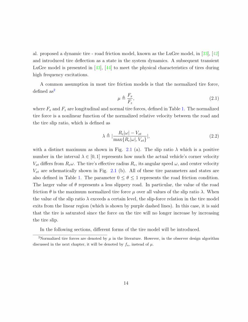
A common assumption in most tire friction models is that the normalized tire force,

defined as2

µ ,FxFz, (2.1)

where Fx and Fz are longitudinal and normal tire forces, defined in Table 1. The normalized

tire force is a nonlinear function of the normalized relative velocity between the road and

the tire slip ratio, which is defined as

λ , | Re|ω| − VxtmaxRe|ω|, Vxt

|, (2.2)

with a distinct maximum as shown in Fig. 2.1 (a). The slip ratio λ which is a positive

number in the interval λ ∈ [0, 1] represents how much the actual vehicle’s corner velocity

Vxt differs from Reω. The tire’s effective radius Re, its angular speed ω, and center velocity

Vxt are schematically shown in Fig. 2.1 (b). All of these tire parameters and states are

also defined in Table 1. The parameter 0 ≤ θ ≤ 1 represents the road friction condition.

The larger value of θ represents a less slippery road. In particular, the value of the road

friction θ is the maximum normalized tire force µ over all values of the slip ratio λ. When

the value of the slip ratio λ exceeds a certain level, the slip-force relation in the tire model

exits from the linear region (which is shown by purple dashed lines). In this case, it is said

that the tire is saturated since the force on the tire will no longer increase by increasing

the tire slip.

In the following sections, different forms of the tire model will be introduced.

2Normalized tire forces are denoted by µ in the literature. However, in the observer design algorithm

discussed in the next chapter, it will be denoted by fn, instead of µ.

14

(𝑏)

𝑉𝑥𝑡

𝜔

𝑅𝑒

Patch length: 𝐿 0 0.1 0.2 0.3 0.4 0.5

0

0.2

0.4

0.6

0.8

1

1.2

1.4

Tire Curves

Dry

𝜃 = 0.9

Wet

𝜃 = 0.5

Ice

𝜃 = 0.2

𝜆

𝜇

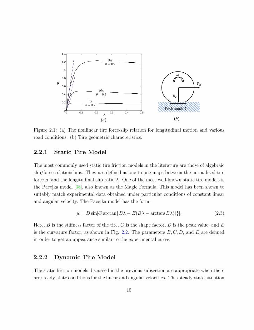
(𝑎)

Figure 2.1: (a) The nonlinear tire force-slip relation for longitudinal motion and various

road conditions. (b) Tire geometric characteristics.

2.2.1 Static Tire Model

The most commonly used static tire friction models in the literature are those of algebraic

slip/force relationships. They are defined as one-to-one maps between the normalized tire

force µ, and the longitudinal slip ratio λ. One of the most well-known static tire models is

the Pacejka model [38], also known as the Magic Formula. This model has been shown to

suitably match experimental data obtained under particular conditions of constant linear

and angular velocity. The Pacejka model has the form:

µ = D sin[C arctanBλ− E(Bλ− arctan(Bλ))], (2.3)

Here, B is the stiffness factor of the tire, C is the shape factor, D is the peak value, and E

is the curvature factor, as shown in Fig. 2.2. The parameters B,C,D, and E are defined

in order to get an appearance similar to the experimental curve.

2.2.2 Dynamic Tire Model

The static friction models discussed in the previous subsection are appropriate when there

are steady-state conditions for the linear and angular velocities. This steady-state situation

15

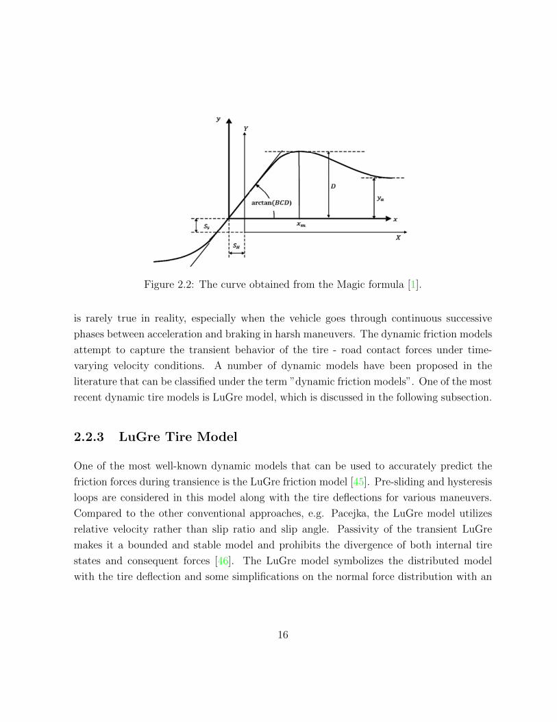
Figure 2.2: The curve obtained from the Magic formula [1].

is rarely true in reality, especially when the vehicle goes through continuous successive

phases between acceleration and braking in harsh maneuvers. The dynamic friction models

attempt to capture the transient behavior of the tire - road contact forces under time-

varying velocity conditions. A number of dynamic models have been proposed in the

literature that can be classified under the term ”dynamic friction models”. One of the most

recent dynamic tire models is LuGre model, which is discussed in the following subsection.

2.2.3 LuGre Tire Model

One of the most well-known dynamic models that can be used to accurately predict the

friction forces during transience is the LuGre friction model [45]. Pre-sliding and hysteresis

loops are considered in this model along with the tire deflections for various maneuvers.

Compared to the other conventional approaches, e.g. Pacejka, the LuGre model utilizes

relative velocity rather than slip ratio and slip angle. Passivity of the transient LuGre

makes it a bounded and stable model and prohibits the divergence of both internal tire

states and consequent forces [46]. The LuGre model symbolizes the distributed model

with the tire deflection and some simplifications on the normal force distribution with an

16

averaged representation of zx for the longitudinal direction as:

zx(t) = Vrx − (σ0|Vrx|θg(Vrx)

+ κRe|ω|)zx(t),

µ = σ0zx(t) + σ1zx(t) + σ2Vrx, (2.4)

where Vrx = Reω − Vxt is the tire relative velocity, and all parameters are defined in the

nomenclature chapter. The function g(Vrx) is defined as

g(Vrx) = µc + (µs − µc) e−|VrxVs|12

(2.5)

In the LuGre model, the tire relative velocity Vrx plays the role of tire slip λ in the static

tire models. The tuning of LuGre tire parameters can be done with experimental curves

of the tire and by utilizing an error cost function and least square techniques. In (2.4),

parameter θ represents the road friction condition. The force distribution along the patch

line is represented by parameter κ in the model (2.4) and can be a function of time, a

constant, or may be approximated by an asymmetric trapezoidal scheme. The suggested

value for κ in [33] is κ = 76L

where L is the tire patch length, shown in Fig. 2.1, (b). It

can also be obtained from an acceptable range of 1.1L≤ κ ≤ 1.4

L.

In the following section, a brief overview of the vehicle’s lateral dynamics is presented.

2.3 Vehicle Lateral Dynamics

In this section, vehicle lateral dynamics is described for both linear and non-linear (using

LuGre tire model) tire model cases. Hence, to develop these dynamics, the knowledge from

the previous section on tire models will be used. The discussion in this section will be used

in the subsequent chapters.

2.3.1 Linear Lateral Dynamics Model

The 2DOF bicycle model, a well-known vehicle lateral model, provides vehicle lateral

velocity and yaw rate based on longitudinal and lateral tire forces, Fx and Fy. The lateral

17

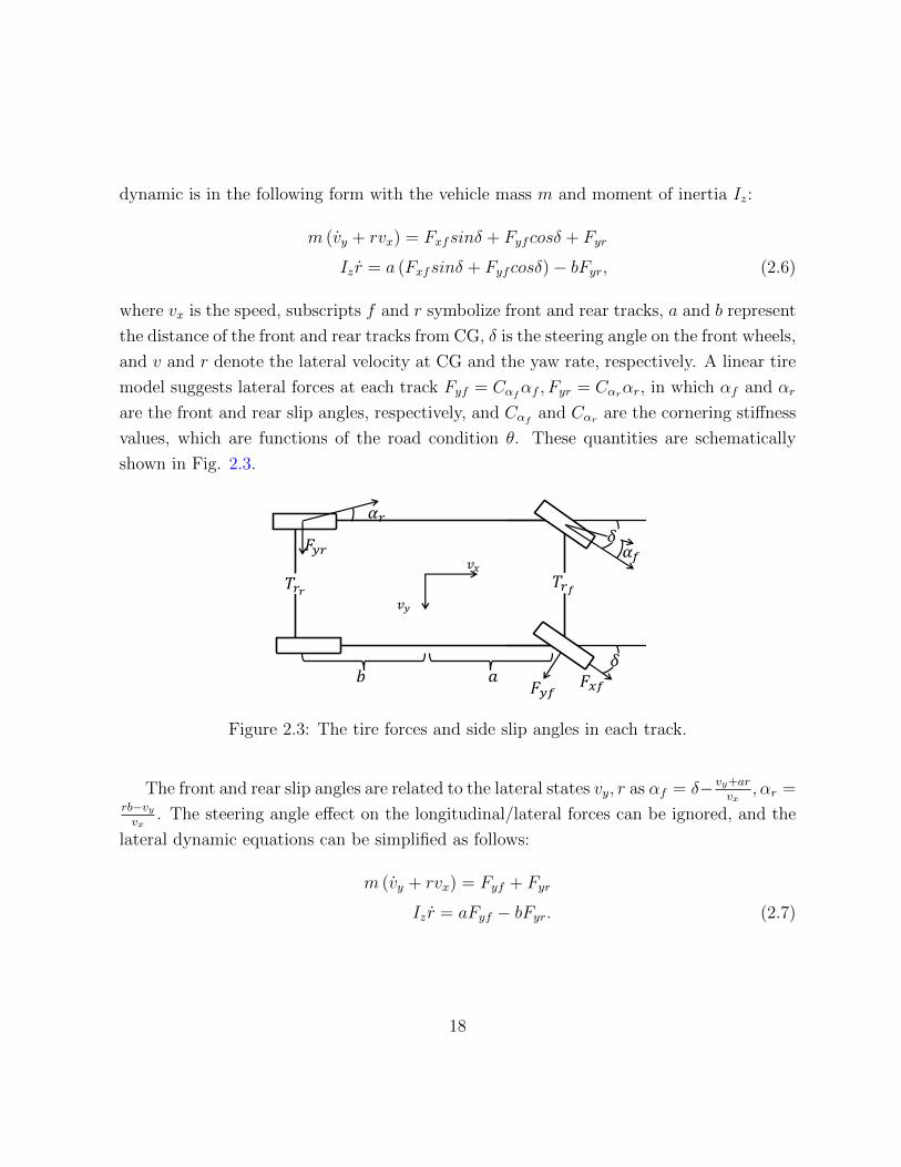
dynamic is in the following form with the vehicle mass m and moment of inertia Iz:

m (vy + rvx) = Fxfsinδ + Fyfcosδ + Fyr

Iz r = a (Fxfsinδ + Fyfcosδ)− bFyr, (2.6)

where vx is the speed, subscripts f and r symbolize front and rear tracks, a and b represent

the distance of the front and rear tracks from CG, δ is the steering angle on the front wheels,

and v and r denote the lateral velocity at CG and the yaw rate, respectively. A linear tire

model suggests lateral forces at each track Fyf = Cαfαf , Fyr = Cαrαr, in which αf and αr

are the front and rear slip angles, respectively, and Cαf and Cαr are the cornering stiffness

values, which are functions of the road condition θ. These quantities are schematically

shown in Fig. 2.3.

𝑣𝑥

𝑣𝑦

𝛿 𝛼𝑓

𝛼𝑟

𝐹𝑦𝑟

𝑏 𝑎

𝑇𝑟𝑓 𝑇𝑟𝑟

𝐹𝑦𝑓 𝐹𝑥𝑓 𝛿

Figure 2.3: The tire forces and side slip angles in each track.

The front and rear slip angles are related to the lateral states vy, r as αf = δ− vy+ar

vx, αr =

rb−vyvx

. The steering angle effect on the longitudinal/lateral forces can be ignored, and the

lateral dynamic equations can be simplified as follows:

m (vy + rvx) = Fyf + Fyr

Iz r = aFyf − bFyr. (2.7)

18

Consequently, the linear tire-vehicle handling model can be represented byvy(t)r(t)

︸ ︷︷ ︸

x

=

−Cαf+Cαr

vxm−(

aCαf−bCαrvxm

+ vx)

−aCαf−bCαrvxIz

−a2Cαf+b2Cαr

vxIz

︸ ︷︷ ︸

A

vy(t)r(t)

+

Cαfm

aCαfIz

︸ ︷︷ ︸

B

δ (2.8)

As pointed out above, the bicycle model is obtained under the assumption that the relation

between the lateral force and slip angle is linear. However, this assumption is not always

realistic. More specifically, the relation between the kinematic variables (e.g., slip ratio or

slip angle) and the forces of the tire is generally nonlinear, as pointed out in the previous

section.

2.3.2 Nonlinear Lateral Dynamics Model

In the previous subsection, a linear tire model is assumed and used to derive the lateral

dynamic equation (2.8). However, this assumption is not realistic due to the nonlinear

nature of tire-road interactions. After discussing the LuGre model in Section 2.2, we

incorporate it into the vehicle lateral dynamics (2.7) in this section. For simplicity, here

we use a steady-state LuGre model to derive the lateral dynamics. It is discussed by detail

in [47] that using steady-state and transient LuGre models provide similar results in lateral

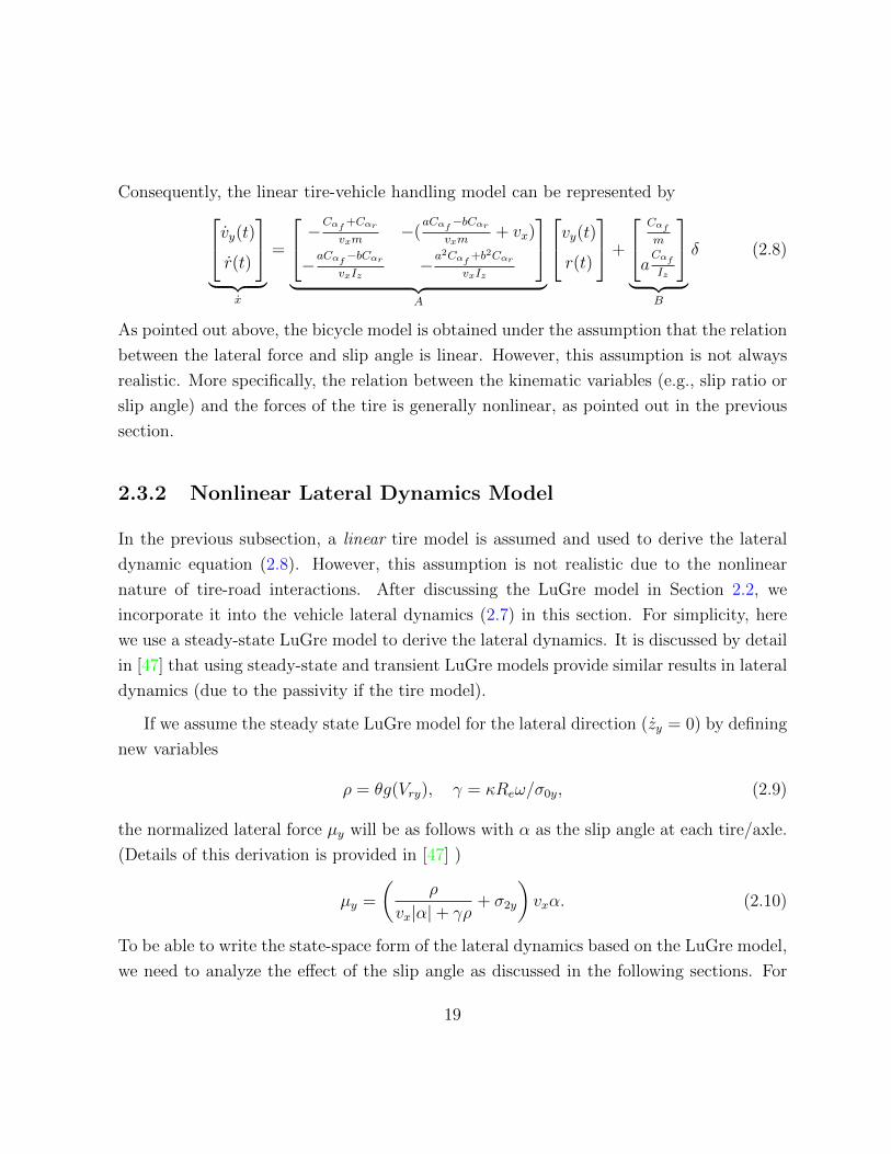
dynamics (due to the passivity if the tire model).

If we assume the steady state LuGre model for the lateral direction (zy = 0) by defining

new variables

ρ = θg(Vry), γ = κReω/σ0y, (2.9)

the normalized lateral force µy will be as follows with α as the slip angle at each tire/axle.

(Details of this derivation is provided in [47] )

µy =

(ρ

vx|α|+ γρ+ σ2y

)vxα. (2.10)

To be able to write the state-space form of the lateral dynamics based on the LuGre model,

we need to analyze the effect of the slip angle as discussed in the following sections. For

19

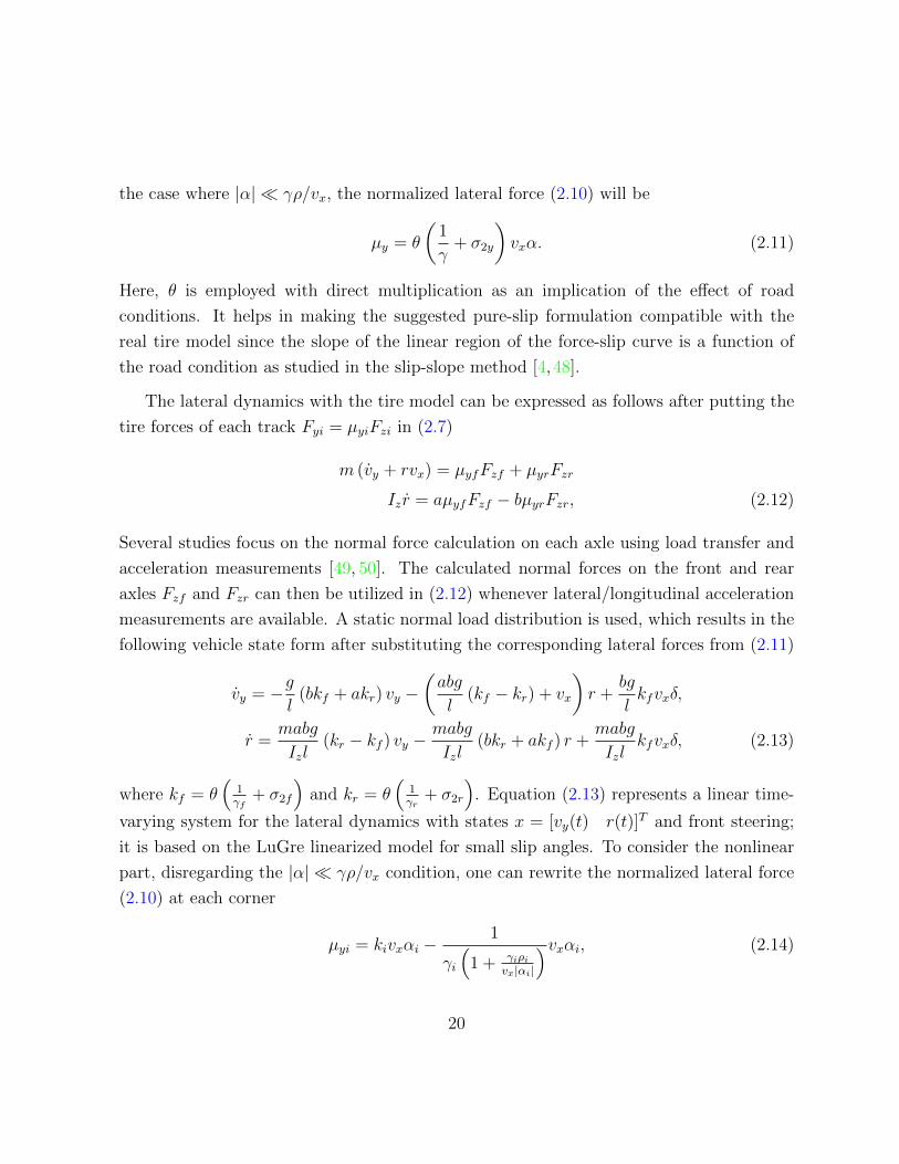
the case where |α| γρ/vx, the normalized lateral force (2.10) will be

µy = θ

(1

γ+ σ2y

)vxα. (2.11)

Here, θ is employed with direct multiplication as an implication of the effect of road

conditions. It helps in making the suggested pure-slip formulation compatible with the

real tire model since the slope of the linear region of the force-slip curve is a function of

the road condition as studied in the slip-slope method [4,48].

The lateral dynamics with the tire model can be expressed as follows after putting the

tire forces of each track Fyi = µyiFzi in (2.7)

m (vy + rvx) = µyfFzf + µyrFzr

Iz r = aµyfFzf − bµyrFzr, (2.12)

Several studies focus on the normal force calculation on each axle using load transfer and

acceleration measurements [49, 50]. The calculated normal forces on the front and rear

axles Fzf and Fzr can then be utilized in (2.12) whenever lateral/longitudinal acceleration

measurements are available. A static normal load distribution is used, which results in the

following vehicle state form after substituting the corresponding lateral forces from (2.11)

vy = −gl

(bkf + akr) vy −(abg

l(kf − kr) + vx

)r +

bg

lkfvxδ,

r =mabg

Izl(kr − kf ) vy −

mabg

Izl(bkr + akf ) r +

mabg

Izlkfvxδ, (2.13)

where kf = θ(

1γf

+ σ2f

)and kr = θ

(1γr

+ σ2r

). Equation (2.13) represents a linear time-

varying system for the lateral dynamics with states x = [vy(t) r(t)]T and front steering;

it is based on the LuGre linearized model for small slip angles. To consider the nonlinear

part, disregarding the |α| γρ/vx condition, one can rewrite the normalized lateral force

(2.10) at each corner

µyi = kivxαi −1

γi

(1 + γiρi

vx|αi|

)vxαi, (2.14)

20

where i ∈ f, r can be front or rear tires, ρi and γi are defined in (2.9), vx is the vehicle

speed, and αi is the slip angle at each track. The term kivxα represents the linear part

(2.11), and the second term shows the nonlinear behavior of the lateral force with respect

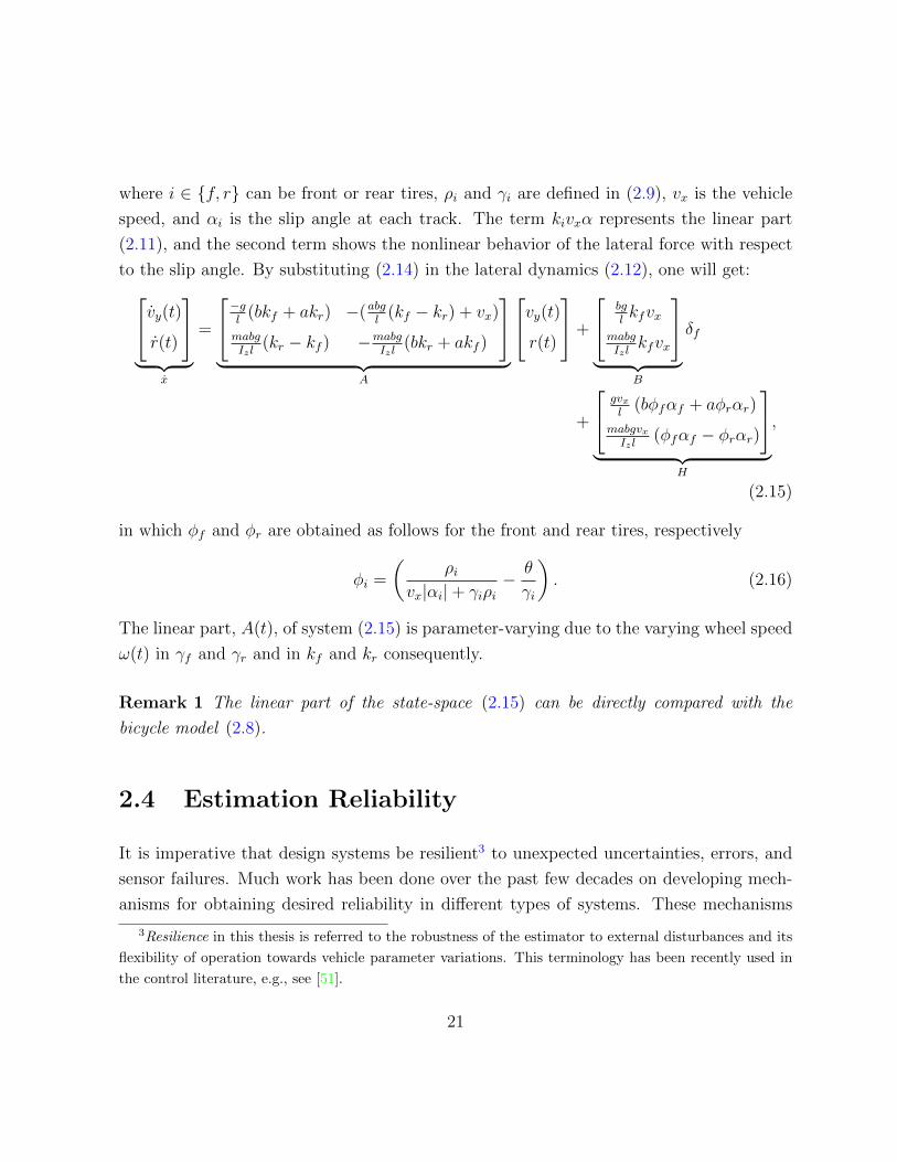
to the slip angle. By substituting (2.14) in the lateral dynamics (2.12), one will get:vy(t)r(t)

︸ ︷︷ ︸

x

=

−gl (bkf + akr) −(abgl

(kf − kr) + vx)

mabgIzl

(kr − kf ) −mabgIzl

(bkr + akf )

︸ ︷︷ ︸

A

vy(t)r(t)

+

bglkfvx

mabgIzl

kfvx

︸ ︷︷ ︸

B

δf

+

gvxl

(bφfαf + aφrαr)

mabgvxIzl

(φfαf − φrαr)

︸ ︷︷ ︸

H

,

(2.15)

in which φf and φr are obtained as follows for the front and rear tires, respectively

φi =

(ρi

vx|αi|+ γiρi− θ

γi

). (2.16)

The linear part, A(t), of system (2.15) is parameter-varying due to the varying wheel speed

ω(t) in γf and γr and in kf and kr consequently.

Remark 1 The linear part of the state-space (2.15) can be directly compared with the

bicycle model (2.8).

2.4 Estimation Reliability

It is imperative that design systems be resilient3 to unexpected uncertainties, errors, and

sensor failures. Much work has been done over the past few decades on developing mech-

anisms for obtaining desired reliability in different types of systems. These mechanisms

3Resilience in this thesis is referred to the robustness of the estimator to external disturbances and its

flexibility of operation towards vehicle parameter variations. This terminology has been recently used in

the control literature, e.g., see [51].

21

range from conceptually simple modular redundancy schemes to more advanced model-

based fault-diagnosis techniques.

The need for a rigorous theory of reliability and fault diagnostics in control systems has

only recently been recognized as a fertile and important area of research. The report in [52]

highlights several key differences in reliability requirements for control systems and tradi-

tional information technology systems. One particularly important differentiating factor is

that control systems involve the regulation of physical processes. This fact imposes hard

real-time constraints on the system since a delay in processing could lead to instabilities

or cascading failures in the control loop, potentially cause severe physical and economic

damage. Papers [53, 54] echo a call for the development of a rigorous theory of reliability

in control systems, and it details several open challenges for research.

To evaluate the performance of a reliable estimator (or controller), one compares the

actual behavior of the estimator to the expected behavior and raises an alarm if the two

deviate. The expected behavior is usually determined from a model of the plant; when

there are disturbances or the model is uncertain, the expected and actual outputs will not

coincide exactly. In such cases, the control system’s designer must determine how different

the two signals are allowed to be before raising an alarm. There is a trade-off here: if the

threshold is set too low, there will be many false alarms, and if the threshold is too high,

some legitimate faults might be missed. The relative weighting of these two factors will

depend on the application at hand. It is important to note that this scheme is called the

real-time fault diagnostics in that it runs concurrently with the system. This is in contrast

to a scheduled fault-diagnosis, where the system is checked at regular intervals according to

some maintenance schedule to ensure that it is operating correctly. Real-time monitoring

is important for safety-critical systems so that a fault does not cause the system to become

unstable or progress to a state where it cannot be repaired.

There are a variety of methods to perform fault-detection. The most straightforward

method is to use physical redundancy: the fault-prone components are replicated, and a

comparison mechanism (e.g., majority voter [55]) is used to determine which components

are operating correctly. This scheme has the benefit of being simple to understand and

implement, but it has the potential to be costly due to the replication of components.

An alternative (or perhaps complementary) approach to diagnose faults is to analyze the

22

behavior of the component over time using a model of how the component is supposed to

behave. This is known as analytical redundancy or temporal redundancy [56]. The goal of

the fault-tolerant and reliable estimator (control) system is to allow the system to gracefully

degrade or continue functioning under failures, and prevent faults from propagating to

other parts of the system. A reliable system design can broadly be broken down into two

objectives [57, 58]

1. Fault detection and identification (FDI): determine whether a fault has occurred,

and isolate the component that has failed.

2. Fault accommodation: take steps to correct for the fault, or reconfigure the system

to avoid the faulty component.

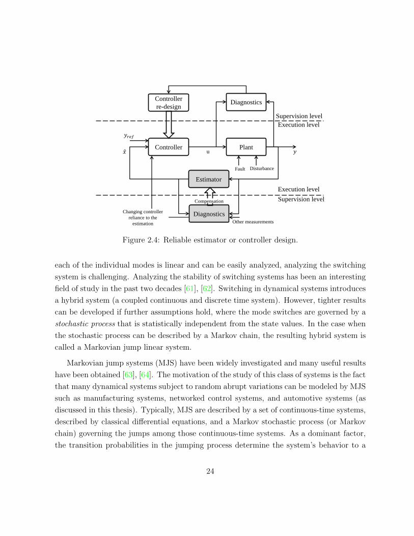
Fig. 2.4 shows a block diagram that illustrates the structure of a fault-tolerant control

system. It is a complete version of what is discussed in [57], and the estimation fault

diagnosis is also added to the block diagram. According to this figure, the detected fault

in the estimation module is either compensated for and corrected or the existence of such

fault is reported to the controller module to change the reliance of the controller to the

estimated signal.

As one of the approaches adopted in this thesis to tackle the reliability of estimators is

the probabilistic and stochastic approach, a literature review of these methods is presented

in the following subsection.

2.4.1 Probabilistic methods in reliable estimator design

The problem of how to deal with uncertainties and unmodeled dynamics in the stability

and performance analysis of dynamical systems has been investigated deeply in the past

decades. Most of the efforts are towards an analysis of robust controller design under

unmodeled dynamics. The main trend in those analyses is to show the exponential (robust)

stability of the nominal system (the system disregarding the unmodeled part) and then

find a (tight) bound for the states of the system in the presence of the unmodeled dynamics

[59, 60]. However, there are times when the system operates in multiple modes. Even if

23

Controller

Estimator

Diagnostics

Diagnostics

Plant

Supervision level

Execution level

Supervision level

Execution level

Controller

re-design

Compensation

Fault Disturbance

𝑦 u 𝑥

𝑦𝑟𝑒𝑓

Other measurements

Changing controller

reliance to the

estimation

Figure 2.4: Reliable estimator or controller design.

each of the individual modes is linear and can be easily analyzed, analyzing the switching

system is challenging. Analyzing the stability of switching systems has been an interesting

field of study in the past two decades [61], [62]. Switching in dynamical systems introduces

a hybrid system (a coupled continuous and discrete time system). However, tighter results

can be developed if further assumptions hold, where the mode switches are governed by a

stochastic process that is statistically independent from the state values. In the case when

the stochastic process can be described by a Markov chain, the resulting hybrid system is

called a Markovian jump linear system.

Markovian jump systems (MJS) have been widely investigated and many useful results

have been obtained [63], [64]. The motivation of the study of this class of systems is the fact

that many dynamical systems subject to random abrupt variations can be modeled by MJS

such as manufacturing systems, networked control systems, and automotive systems (as

discussed in this thesis). Typically, MJS are described by a set of continuous-time systems,

described by classical differential equations, and a Markov stochastic process (or Markov

chain) governing the jumps among those continuous-time systems. As a dominant factor,

the transition probabilities in the jumping process determine the system’s behavior to a

24

large extent, and so far, many analysis and synthesis results have been reported assuming

the complete knowledge of the transition probabilities. Recently, an interesting extension

to this research is in considering the uncertain transition probabilities, which aims to

utilize robust methodologies to deal with the norm-bounded or polytopic uncertainties

presumed in the transition probabilities, see for example [65], [66]. Ideal knowledge of the

transition probabilities are definitely expected to simplify the system analysis and design,

however, the likelihood of obtaining such available knowledge is actually questionable and

probably expensive. A typical example can be found in network control systems, where

the packet dropouts and channel delays are well-known to be modeled by Markov Chains

with the usual assumption that all the transition probabilities are completely accessible

[67], [68], [69]. In this thesis, much attention is focused on using this methodology in

designing a reliable estimator in the presence of faulty measurements as well as analyzing

the robustness of the observer toward unknown changes in the system parameters. The

faulty measurements are equivalent to the dropped packets in network control systems,

and the stability of the resulting hybrid system is analyzed.

2.5 Summary

A comprehensive literature review on vehicle estimation, including vehicle tire forces and

velocities, was discussed in this chapter. Moreover, a detailed review of the works done in

the field of road friction identification was done and the problems in each approach was also

discussed. Beyond introducing recent research on vehicle state and road condition estima-

tion, a brief overview of the vehicle tire model as well as vehicle handling dynamics was

also introduced, which will be used in the subsequent chapters. Lastly, recent approaches

to reliability and fault detection and identification algorithms for estimation and control

of dynamical systems were discussed.

25

Chapter 3

Vehicle Corner Velocity Estimation

In Chapter 1, the necessity and importance of having a reliable estimation of vehicle veloc-

ity was discussed and the efforts done in studying this subject and challenges that should

be overcome were reviewed. To this end, an algorithm for estimating vehicle corner velocity

is introduced in this chapter. In this algorithm, a vehicle kinematics (tire-free) approach is

coupled with the tire’s internal states at each corner to estimate relative velocities of the

tires as in [70–73]. The selected tire model is the average lumped LuGre [43] because of

the dynamics in the internal deflection state as described briefly in the following subsec-

tion. The vehicle and tire parameters (with their actual values used for experiments) are

presented in Table 1.

3.1 Longitudinal Velocity Estimation

The LuGre tire model was introduced in detail in Chapter 2 and here, we briefly review

the dynamics that are used for the velocity estimator design. The internal longitudinal and

lateral states zq (q ∈ x, y)1 and the normalized tire forces fnq (i.e. fnx = Fx/Fz, fny =

1From now, an index q for tire states or parameters indicates the direction of interest, i.e. q ∈ x, y.Tire forces and velocities in tire coordinates are shown in Fig. 3.3 (b).

26

Fy/Fz) in the pure-slip case are described as follows in the LuGre model:

zq = Vrq − (κqRe|ω|+σ0q|Vrq|θg(Vrq)

)zq, (3.1)

fnq = σ0qzq + σ1qzq + σ2qVrq, (3.2)

in which ω is the wheel speed and Vrx = Reω−Vxt, Vry = −Vyt are the longitudinal/lateral

relative velocities. The tires’ center velocities in the tire coordinates are denoted by Vxt,

Vyt. The function, g(Vrq) in the pure-slip model is defined as g(Vrq) = µc+(µs−µc)e−|VrqVs|0.5 .

The effect of pure and combined-slip LuGre tire models in the vehicle stability is explored

in [47]. The parameter θ ∈ [0, 1] in (3.1) represents the road condition; this value is small

when the road is slippery and it is close to 1 otherwise. In the following subsection, θ is

assumed to be unknown resulting in the unknown term σ0q |Vrq |θg(Vrq)

zq in (3.1).

Assuming the unknown road friction term %zx = σ0q |Vrq |θg(Vrq)

zq as the bounded uncertainty,

one can write the LuGre model (3.1) as follows at each corner for the longitudinal direction:

zx = Vrx − κxRe|ω|zx + %zx. (3.3)

The time derivative of the longitudinal relative velocity is described as:

Vrx = Reω − Vxt. (3.4)

However, the measured signals2 Vxt and ω (and particularly its derivative ω) are corrupted

due to the sensor noises and bias. The deviation of the measured relative acceleration

Reω − Vxt from Vrx at each corner due to the sensor noises is denoted by %ax and we have

Vrx = Reω − Vxt + %ax. (3.5)

Dynamics of the tires’ internal states (3.3) together with relative velocities (3.5) are used

to develop the following dynamics:

x =

−κxRe|ω| 1

0 0

︸ ︷︷ ︸

Ax(ω)

x + Bxux + %x, (3.6)

2The value of the longitudinal acceleration at CG (measured by IMU) is projected into the tires’ center

Vxt.

27

in which Bx = [0 1]T , uncertainties are denoted by %x = [%zx %ax]T , the states are

x = [zx Vrx]T , and ux = Reω − Vxt. By substituting zx from (3.3) into the normalized

longitudinal force of the pure-slip case (3.2), one can rewrite the output equation as:

fnx = [(σ0x − σ1xκxRe|ω|) (σ1x + σ2x)]x + σ1x%zx

= Cx(ω)x + σ1x%zx. (3.7)

By employing the normalized longitudinal force (3.7) and the system (3.6), the following

observer is obtained for a longitudinal velocity estimation with the estimated output y =

fnx = Cx(ω)x and observer gains Lx = [L1x L2x]T :

˙x = Ax(ω)x + Bxux + Lx(fnx − fnx), (3.8)

where fnx = Fx/Fz is the normalized longitudinal tire force. The bounded time-varying

parameter in (3.8) is the wheel speed and the parameter varying state transition matrix is

Ax(ω) ∈ R2×2. The error dynamics ex = x− x from (3.6) and (3.8) yields:

ex = [Ax(ω)− LxCx]ex − Lxσ1x%zx + %x

= Aex(ω)ex +

1− L1xσ1x 0

−L2xσ1x 1

%x= Aex(ω)ex + Bex%x. (3.9)

The system matrix Ax(ω) in (3.8) is physically bounded; thus, a conventional observability

test is performed. The observability matrix for parameter-varying systems like (3.6) with

output (3.7) is given by [74] as:

On = [ε1 ε2... εn]T ,

ε1 = Cx, εi+1 = εiAx(ω) + εi. (3.10)

Observability is confirmed by holding the full rank condition rank(O2) = 2 at each fixed

time span for the operating regions of the wheel speed and its time derivatives. Thus,

the parameter-varying system (3.6) with output (3.7) is observable, and it is feasible to

estimate the tires’ longitudinal internal states zx and the relative velocity Vrx by employing

the longitudinal force as the output.

28

Remark 2 For implementation and road experiments, discretization of the continuous-

time system (3.6) with the output y = Cxx + Dxux is done by the Step-Invariance method

because of its precision and response characteristics. The step-invariance discretization is

the zero-order hold method and includes a constant input signal ux(t) during integration.

It has good accuracy with the platform sampling frequency of 200[Hz]. Moreover, the

richness of the step signal, in terms of the frequencies that it carries, makes the step

invariance method very suitable for automotive applications as there exist a large amount

of uncertainties and disturbances. The input of the continuous-time system is the hold

signal ux[k] = ux[tk] for a period between tk ≤ t < tk+1 with the sample time Ts. Then,

the discrete-time system x[k + 1] = Adx[k]x[k] + Bd

xux[k], y[k] = Cdxx[k] + Dd

xux[k] has the

output matrices Cdx = Cx,D

dx = Dx and state/input matrices:

Adx = eAx(t)Ts , Bd

x =

∫ Ts

0

eAx(t)τBx(t)dτ. (3.11)

The discretized from of the error dynamics (3.9), can now be written as ex[k + 1] =

Adex [k]ex[k] + Bd

ex%x[k]. The following subsection focuses on the corner-based velocity ob-

server for the lateral direction.

3.2 Lateral Velocity Estimation

The LuGre output equation (3.2) for the lateral direction can be expressed as follows:

fny = [(σ0y − σ1yκyRe|ω|) (σ1y + σ2y)]x + σ1y%zy

= Cy(ω)x + σ1y%zy, (3.12)

where the states are x = [zy Vry]T . The relative lateral acceleration Vry = −Vyt+%ay (the

projected lateral acceleration in the tire coordinate system is denoted by Vyt, compensated

by road angles from a real-time road angle estiamtor [75]) is combined with the lateral

LuGre internal state to form the lateral velocity estimator. Equation (3.6) can be rewritten

29

for the lateral direction as

˙x =

−κyRe|ω| 1

0 0

︸ ︷︷ ︸

Ay(ω)

x + Byuy + %x, (3.13)

where By = Bx, and uy = −vyt. Uncertainties in the lateral states are denoted by %y =

[%zy %ay]T . The state estimator can be expressed as follows for the lateral direction with

the output yl = fny = Cy(ω)xl:

˙x = Ay(ω)ˆx + Byuy + Ly(fny − fny), (3.14)

in which Ly = [L1y L2y]T .

Remark 3 Similar to the longitudinal direction, the observability of the lateral direction

dynamics can be verified by the observability criterion (3.10) for the parameter-varying

system with Ay(ω),Cy(ω).

The error dynamics is then derived as follows for the lateral velocity estimator and repre-

sents a linear parameter varying system:

ey = Aey(ω)ey +

1− L1yσ1y 0

−L2yσ1y 1

︸ ︷︷ ︸

Bey

%y, (3.15)

where Aey = [Ay(ω) − LyCy]. The error dynamics in discrete-time yields ey[k + 1] =

Adey [k]ey[k] + Bd

ey%y[k]. In order to increase the accuracy of the velocity estimation at

each corner, the effect of the suspension compliance is considered on the estimators and is

discussed in the following section.

In the above analysis, we assumed the vehicle as a solid (rigid) body and there is no

relative motion between its parts. However, in estimating the slip of the tire, it is important

to consider the extra degree of freedom that exists between the chassis and the wheel due to

the suspension compliance. Modeling and analyzing the effect of the suspension compliance

on the vehicle corner velocity estimation is the subject of the following section.

30

3.3 Model improvement by Inclusion of Suspension

Compliance

As discussed in Chapter 1, one of the sources of inaccuracy in vehicle velocity estimation

are unmodeled dynamics which are not included in the design of the observer. One of

the examples of such inaccuracies in the dynamics is the effect of extra dynamics (relative

motion) between the wheel and the vehicle chassis due to the existence of suspension

compliance. In this chapter, the effect of the suspension compliance on the vehicle’s corner

velocity estimation is analyzed. It is worth noting that this effect is not captured by GPS

measurements as GPS only provides the vehicle’s velocity at CG. Thus, analyzing the effect

of the suspension dynamics in both longitudinal and lateral directions is vital for having a

more accurate estimation of the tire slip.

3.3.1 Suspension Model

The extra degree of freedom between the chassis and the tire due to the suspension com-

pliance follows specific dynamics. This dynamics can be represented by a second-order

system as:

Muψx(t) + Cxψx(t) +Kxψx(t) = Fx

Muψy(t) + Cyψy(t) +Kyψy(t) = Fy, (3.16)

where Fx and Fy are longitudinal and lateral forces on each tire, Kx and Ky are the

equivalent stiffness of the suspension compliance in each direction, Cx and Cy are the

equivalent damping of the suspension compliance in each direction and Mu is the quarter

car unsprung mass. Displacements due to the suspension in each direction, are denoted by

ψx(t) and ψy(t). The suspension dynamics at each corner can be written in the following

state space form: ψq(t)ψq(t)

=

0 1

−KqMu

−CqMu

ψq(t)ψq(t)

+

0

1

FqMu

, (3.17)

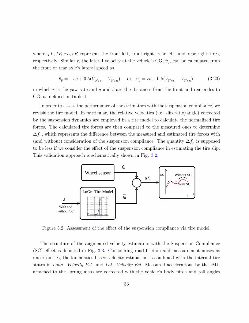
31

where q ∈ x, y is used for brevity. The velocity term ψq(t) should be directly added

to the estimated velocity at each corner due to the dynamics (3.17). This procedure is

discussed in detail bellow:

The estimated relative velocities Vrx and Vry by (3.8), (3.14) are used for the longitudinal

velocity estimation at the tire coordinates as Vxt = Reω− Vrx and Vyt = −Vry. Afterwards,

utilizing the steering angle δ at the front and rear tracks (i.e. δ = 0 for the rear track of

front-steering vehicles) and each corner’s velocity in the vehicle coordinates yields ˆVxc =

Vxt cos δ− Vyt sin δ for the longitudinal direction and ˆVyc = Vxt sin δ+ Vyt cos δ for the lateral

direction. To account for suspension compliance, the velocities (3.17) are then added to

the estimated velocities in the vehicle coordinates as:

Vxc = ˆVxc + ψx, Vyc = ˆVyc + ψy. (3.18)

The above procedure is schematically shown in Fig. 3.1. Estimated corner velocities, Vxc

𝐶𝑦

𝐾𝑥

𝐶𝑥

𝐾𝑦

𝑉 𝑦𝑐 = (𝑉 𝑥𝑡 sin 𝛿 + 𝑉 𝑦𝑡 cos 𝛿) + 𝜓 𝑦

𝑉 𝑦𝑐

𝑉 𝑥𝑐 = (𝑉 𝑥𝑡 cos 𝛿 − 𝑉 𝑦𝑡 sin 𝛿) + 𝜓 𝑥

𝑉 𝑥𝑐

Figure 3.1: The effect of the suspension compliance on the vehicle corner velocities are

schematically represented by spring and dampers.

and Vyc, are then used for calculation of the vehicle’s velocity at CG. The longitudinal

velocity of the vehicle at its CG, called vx, is calculated by the front or the rear axle speed

via

vx = 0.5(VxcfL + VxcfR), or vx = 0.5(VxcrL + VxcrR), (3.19)

32

where fL, fR, rL, rR represent the front-left, front-right, rear-left, and rear-right tires,

respectively. Similarly, the lateral velocity at the vehicle’s CG, vy, can be calculated from

the front or rear axle’s lateral speed as

vy = −ra+ 0.5(VycfL + VycfR), or vy = rb+ 0.5(VycrL + VycrR), (3.20)

in which r is the yaw rate and a and b are the distances from the front and rear axles to

CG, as defined in Table 1.

In order to assess the performance of the estimators with the suspension compliance, we

revisit the tire model. In particular, the relative velocities (i.e. slip ratio/angle) corrected

by the suspension dynamics are employed in a tire model to calculate the normalized tire

forces. The calculated tire forces are then compared to the measured ones to determine

∆fn, which represents the difference between the measured and estimated tire forces with

(and without) consideration of the suspension compliance. The quantity ∆fn is supposed

to be less if we consider the effect of the suspension compliance in estimating the tire slip.

This validation approach is schematically shown in Fig. 3.2.

Wheel sensor

LuGre Tire Model

𝜆 𝑓𝑛

𝑓𝑛

Δ𝑓𝑛 Δ𝑓𝑛

𝑡

Without SC

With SC

With and

without SC

Figure 3.2: Assessment of the effect of the suspension compliance via tire model.

The structure of the augmented velocity estimators with the Suspension Compliance

(SC) effect is depicted in Fig. 3.3. Considering road friction and measurement noises as

uncertainties, the kinematics-based velocity estimation is combined with the internal tire

states in Long. Velocity Est. and Lat. Velocity Est. Measured accelerations by the IMU

attached to the sprung mass are corrected with the vehicle’s body pitch and roll angles

33

to include only the kinematics of the motion. These corrected values are then used in the

velocity estimators. A high-slip detection algorithm is used for appropriate observer gain

switch to tackle the slippery cases, which will be discussed in the next chapter. Estimated

corner velocities are augmented with the suspension effect and mapped onto the vehicle’s

CG in the SC and Mapping module.

Remark 4 Tire forces can be measured by wheel sensors. However, because of high cost

impact on mass production vehicles, installation problems, and maintenance issues, tire

force estimation has extensively been tried only in the literature. Longitudinal and lateral

tire forces at each corner can be estimated using nonlinear and sliding mode observers [3],

unknown input observers [8, 10], or Kalman Filter based estimators [5–7]. Normalized

longitudinal and lateral forces fnx, fny are assumed to be known from the Kalman Filter

based estimation on wheel and lateral dynamics [7, 50]. Due to the fact that the vehicle’s

normal force has a significant impact on the normalized longitudinal and lateral tire forces,

a detailed study on tire normal force calculation is done in [50]. Since tire forces are used

as measurements for the velocity estimation in this thesis, they are referred to as force

measurement and force estimation interchangeably.

The experimental validation of the proposed corner-based vehicle velocity observer

together with consideration of the effect of the suspension compliance are discussed in

the following section. The estimated vehicle velocities are compared with those of GPS

measurements for various maneuvers on different road conditions. Moreover, it will be

shown that the effect of the suspension compliance is during harsh traction and braking

maneuvers where the applied tire forces are considerable. Such effect in a tiny time interval

plays an important role in detecting tire slip more accurately and consequently, on vehicle

traction and stability control.

3.4 Experimental Validation

This section demonstrates various experimental results to validate the corner-based vehicle

velocity estimation introduced in the beginning of the chapter. Moreover, the effect of

34

𝑣 𝑥 , 𝑣 𝑦 𝑉 𝑥𝑐 , 𝑉 𝑦𝑐

Figure 3.3: Overall vehicle velocity estimation structure with SC.

considering the suspension compliance on the accuracy of the resulting velocity estimation

is experimentally examined. The estimated vehicle velocities are compared with those

of GPS measurements for various maneuvers on different road conditions. Moreover, it

will be shown that the effect of the suspension compliance is considerable during harsh

traction and braking maneuvers, where the applied tire forces are considerable. Such

effect in a tiny time interval plays an important role in detecting tire slip more accurately

and consequently, on vehicle traction and stability control. Before we start showing the

experimental results, in the following subsection, we introduce the test facilities which are

used together with the empirical approach taken to test the proposed velocity estimation

algorithm.

35

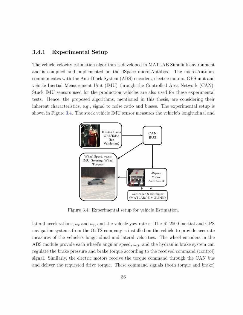
3.4.1 Experimental Setup

The vehicle velocity estimation algorithm is developed in MATLAB Simulink environment

and is compiled and implemented on the dSpace micro-Autobox. The micro-Autobox

communicates with the Anti-Block System (ABS) encoders, electric motors, GPS unit and

vehicle Inertial Measurement Unit (IMU) through the Controlled Area Network (CAN).

Stuck IMU sensors used for the production vehicles are also used for these experimental

tests. Hence, the proposed algorithms, mentioned in this thesis, are considering their

inherent characteristics, e.g., signal to noise ratio and biases. The experimental setup is

shown in Figure 3.4. The stock vehicle IMU sensor measures the vehicle’s longitudinal and

RT2500 6-axis GPS/IMU

(for Validation)

CAN BUS

Controller & Estimator (MATLAB/ SIMULINK)

dSpace Micro-

AutoBox II

Wheel Speed, 3-axis IMU, Steering, Wheel

Torques

Figure 3.4: Experimental setup for vehicle Estimation.

lateral accelerations, ax and ay, and the vehicle yaw rate r. The RT2500 inertial and GPS

navigation systems from the OxTS company is installed on the vehicle to provide accurate

measures of the vehicle’s longitudinal and lateral velocities. The wheel encoders in the

ABS module provide each wheel’s angular speed, ωij, and the hydraulic brake system can

regulate the brake pressure and brake torque according to the received command (control)

signal. Similarly, the electric motors receive the torque command through the CAN bus

and deliver the requested drive torque. These command signals (both torque and brake)

36

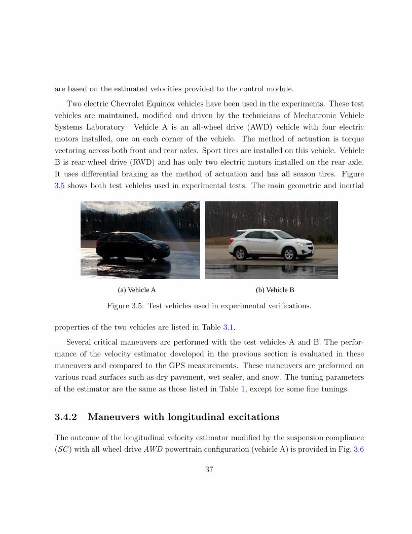
are based on the estimated velocities provided to the control module.

Two electric Chevrolet Equinox vehicles have been used in the experiments. These test

vehicles are maintained, modified and driven by the technicians of Mechatronic Vehicle

Systems Laboratory. Vehicle A is an all-wheel drive (AWD) vehicle with four electric

motors installed, one on each corner of the vehicle. The method of actuation is torque

vectoring across both front and rear axles. Sport tires are installed on this vehicle. Vehicle

B is rear-wheel drive (RWD) and has only two electric motors installed on the rear axle.

It uses differential braking as the method of actuation and has all season tires. Figure

3.5 shows both test vehicles used in experimental tests. The main geometric and inertial

(a) Vehicle A (b) Vehicle B

Figure 3.5: Test vehicles used in experimental verifications.

properties of the two vehicles are listed in Table 3.1.

Several critical maneuvers are performed with the test vehicles A and B. The perfor-

mance of the velocity estimator developed in the previous section is evaluated in these

maneuvers and compared to the GPS measurements. These maneuvers are preformed on

various road surfaces such as dry pavement, wet sealer, and snow. The tuning parameters

of the estimator are the same as those listed in Table 1, except for some fine tunings.

3.4.2 Maneuvers with longitudinal excitations

The outcome of the longitudinal velocity estimator modified by the suspension compliance

(SC ) with all-wheel-drive AWD powertrain configuration (vehicle A) is provided in Fig. 3.6

37

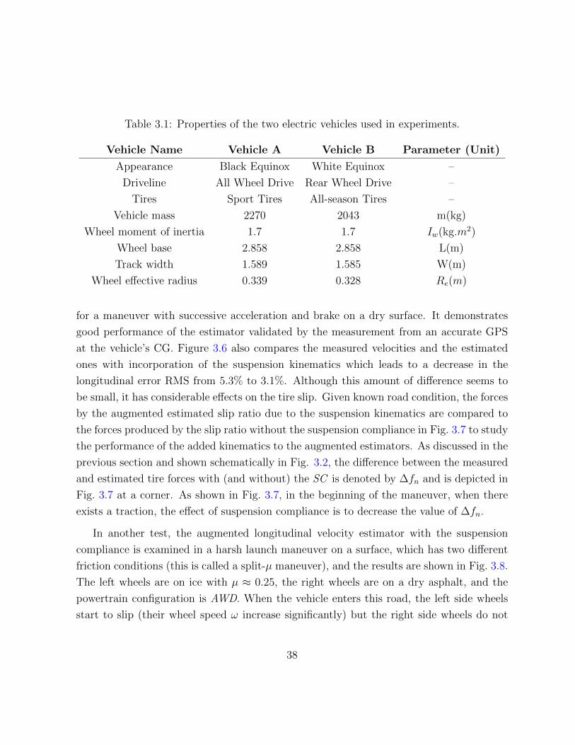
Table 3.1: Properties of the two electric vehicles used in experiments.

Vehicle Name Vehicle A Vehicle B Parameter (Unit)

Appearance Black Equinox White Equinox –

Driveline All Wheel Drive Rear Wheel Drive –

Tires Sport Tires All-season Tires –

Vehicle mass 2270 2043 m(kg)

Wheel moment of inertia 1.7 1.7 Iw(kg.m2)

Wheel base 2.858 2.858 L(m)

Track width 1.589 1.585 W(m)

Wheel effective radius 0.339 0.328 Re(m)

for a maneuver with successive acceleration and brake on a dry surface. It demonstrates

good performance of the estimator validated by the measurement from an accurate GPS

at the vehicle’s CG. Figure 3.6 also compares the measured velocities and the estimated

ones with incorporation of the suspension kinematics which leads to a decrease in the

longitudinal error RMS from 5.3% to 3.1%. Although this amount of difference seems to

be small, it has considerable effects on the tire slip. Given known road condition, the forces

by the augmented estimated slip ratio due to the suspension kinematics are compared to

the forces produced by the slip ratio without the suspension compliance in Fig. 3.7 to study

the performance of the added kinematics to the augmented estimators. As discussed in the

previous section and shown schematically in Fig. 3.2, the difference between the measured

and estimated tire forces with (and without) the SC is denoted by ∆fn and is depicted in

Fig. 3.7 at a corner. As shown in Fig. 3.7, in the beginning of the maneuver, when there

exists a traction, the effect of suspension compliance is to decrease the value of ∆fn.

In another test, the augmented longitudinal velocity estimator with the suspension

compliance is examined in a harsh launch maneuver on a surface, which has two different

friction conditions (this is called a split-µ maneuver), and the results are shown in Fig. 3.8.

The left wheels are on ice with µ ≈ 0.25, the right wheels are on a dry asphalt, and the

powertrain configuration is AWD. When the vehicle enters this road, the left side wheels

start to slip (their wheel speed ω increase significantly) but the right side wheels do not

38

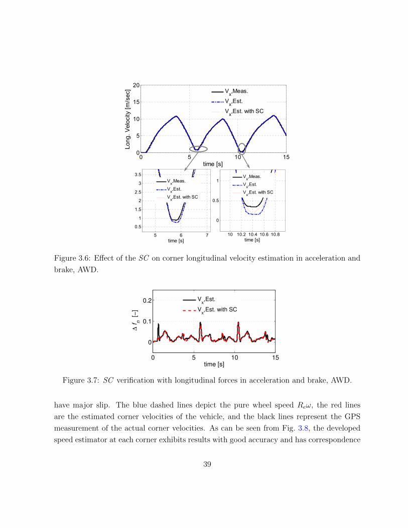
AWD, Accel_Brake_Dry_20140417_006

10 10.2 10.4 10.6 10.8

0

0.5

1

time [s]

Vx,Meas.

Vx,Est.

Vx,Est. with SC

5 6 7

0.5

1

1.5

2

2.5

3

3.5

time [s]

Vx,Meas.

Vx,Est.

Vx,Est. with SC

0 5 10 150

5

10

15

20

time [s]

Long

. Vel

ocity

[m/s

ec]

Vx,Meas.

Vx,Est.

Vx,Est. with SC

Figure 3.6: Effect of the SC on corner longitudinal velocity estimation in acceleration and

brake, AWD.

0 5 10 15

0

0.1

0.2

time [s]

∆ f

n [−

]

Vx,Est.

Vx,Est. with SC

Figure 3.7: SC verification with longitudinal forces in acceleration and brake, AWD.

have major slip. The blue dashed lines depict the pure wheel speed Reω, the red lines

are the estimated corner velocities of the vehicle, and the black lines represent the GPS

measurement of the actual corner velocities. As can be seen from Fig. 3.8, the developed

speed estimator at each corner exhibits results with good accuracy and has correspondence

39

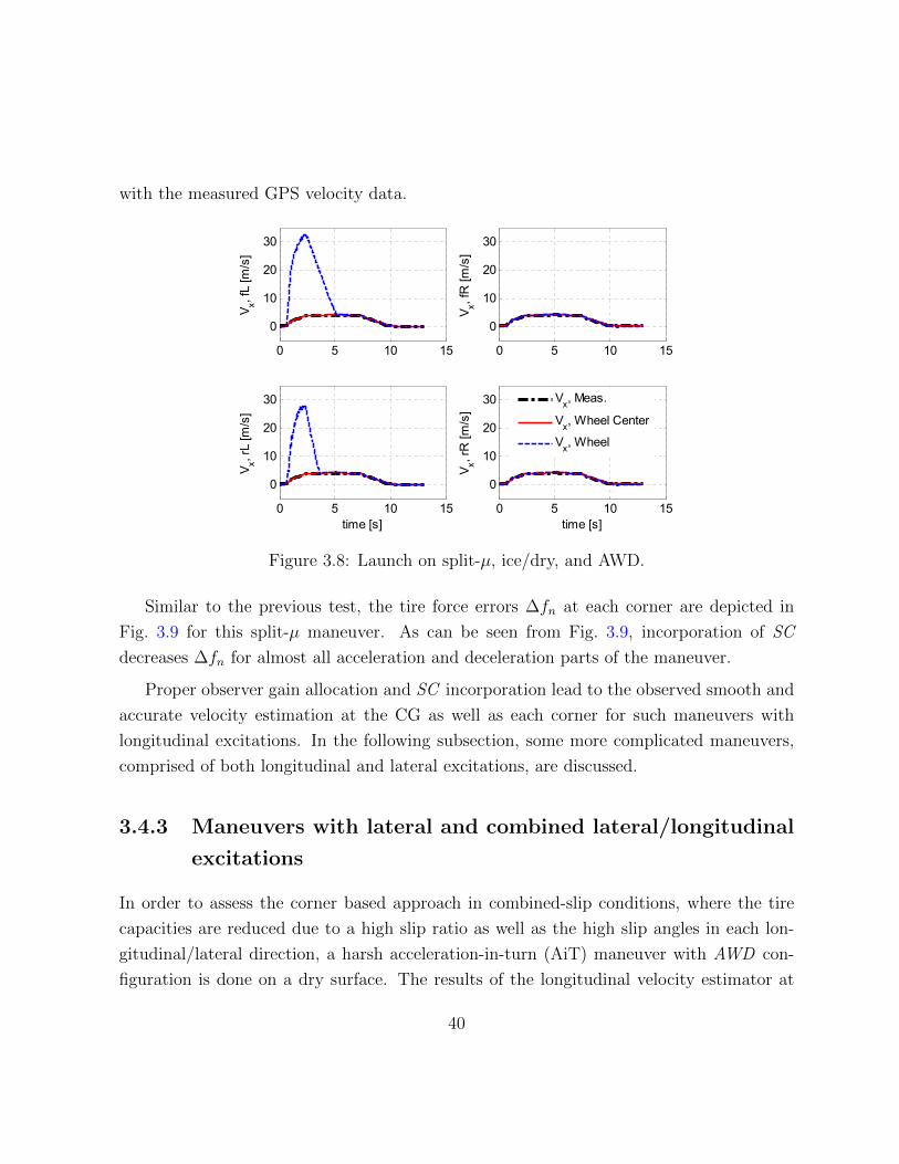
with the measured GPS velocity data.Split , AWD, 20140818_010

Used for VxVy_susp

0 5 10 15

0

10

20

30V x, f

L [m

/s]

0 5 10 15

0

10

20

30

V x, fR

[m/s

]

0 5 10 15

0

10

20

30

V x, rL

[m/s

]

time [s]0 5 10 15

0

10

20

30

V x, rR

[m/s

]

time [s]

Vx, Meas.

Vx, Wheel Center

Vx, Wheel

Figure 3.8: Launch on split-µ, ice/dry, and AWD.

Similar to the previous test, the tire force errors ∆fn at each corner are depicted in

Fig. 3.9 for this split-µ maneuver. As can be seen from Fig. 3.9, incorporation of SC

decreases ∆fn for almost all acceleration and deceleration parts of the maneuver.

Proper observer gain allocation and SC incorporation lead to the observed smooth and

accurate velocity estimation at the CG as well as each corner for such maneuvers with

longitudinal excitations. In the following subsection, some more complicated maneuvers,

comprised of both longitudinal and lateral excitations, are discussed.

3.4.3 Maneuvers with lateral and combined lateral/longitudinal

excitations

In order to assess the corner based approach in combined-slip conditions, where the tire

capacities are reduced due to a high slip ratio as well as the high slip angles in each lon-

gitudinal/lateral direction, a harsh acceleration-in-turn (AiT) maneuver with AWD con-

figuration is done on a dry surface. The results of the longitudinal velocity estimator at

40

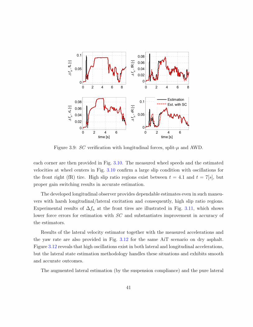
Split , AWD, 20140818_010, zoomed

Used for VxVy_susp

0 2 4 6 80

0.05

0.1

f n ,

fL [-

]

0 2 4 6 8

0

0.02

0.04

0.06

0.08

f n ,

fR [-

]0 2 4 6

0

0.02

0.04

0.06

0.08

f n ,

rL [-

]

time [s]0 2 4 6

0

0.05

0.1

f n ,

rR [-

]time [s]

EstimationEst. with SC

Figure 3.9: SC verification with longitudinal forces, split-µ and AWD.

each corner are then provided in Fig. 3.10. The measured wheel speeds and the estimated

velocities at wheel centers in Fig. 3.10 confirm a large slip condition with oscillations for

the front right (fR) tire. High slip ratio regions exist between t = 4.1 and t = 7[s], but

proper gain switching results in accurate estimation.

The developed longitudinal observer provides dependable estimates even in such maneu-

vers with harsh longitudinal/lateral excitation and consequently, high slip ratio regions.

Experimental results of ∆fn at the front tires are illustrated in Fig. 3.11, which shows

lower force errors for estimation with SC and substantiates improvement in accuracy of

the estimators.

Results of the lateral velocity estimator together with the measured accelerations and

the yaw rate are also provided in Fig. 3.12 for the same AiT scenario on dry asphalt.

Figure 3.12 reveals that high oscillations exist in both lateral and longitudinal accelerations,

but the lateral state estimation methodology handles these situations and exhibits smooth

and accurate outcomes.

The augmented lateral estimation (by the suspension compliance) and the pure lateral

41

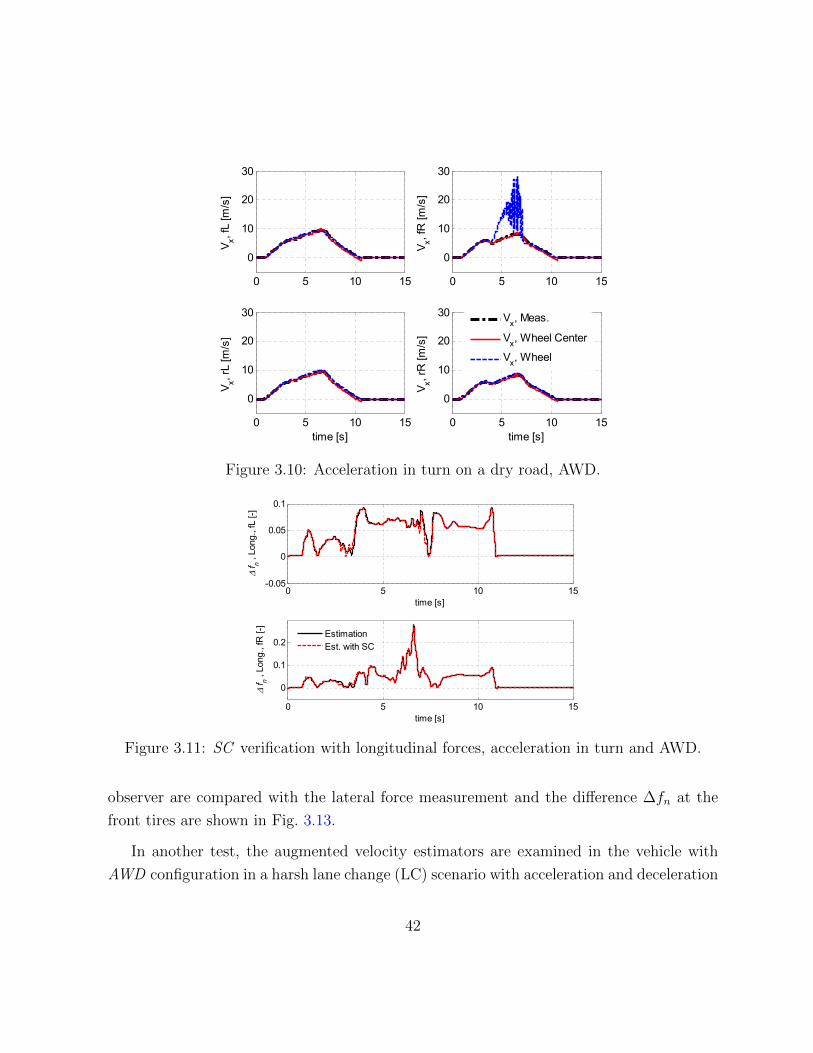
0 5 10 15

0

10

20

30

V x, fL

[m/s

]

0 5 10 15

0

10

20

30

V x, fR

[m/s

]0 5 10 15

0

10

20

30

V x, rL

[m/s

]

time [s]0 5 10 15

0

10

20

30

V x, rR

[m/s

]time [s]

Vx, Meas.

Vx, Wheel Center

Vx, Wheel

4WD, AiT on dry_20140417_test011

Figure 3.10: Acceleration in turn on a dry road, AWD.

0 5 10 15-0.05

0

0.05

0.1

f n ,

Long

., fL

[-]

time [s]

0 5 10 15

0

0.1

0.2

f n ,

Long

., fR

[-]

time [s]

EstimationEst. with SC

4WD, AiT on dry_20140417_test011

Figure 3.11: SC verification with longitudinal forces, acceleration in turn and AWD.

observer are compared with the lateral force measurement and the difference ∆fn at the

front tires are shown in Fig. 3.13.

In another test, the augmented velocity estimators are examined in the vehicle with

AWD configuration in a harsh lane change (LC) scenario with acceleration and deceleration

42

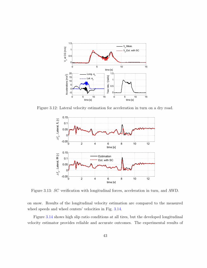
0 5 10 15

0

0.5

1

1.5

V y at C

G [m

/s]

time [s]

Vy,Meas.

Vy,Est. with SC

0 5 10 15

-50

5101520

Acc

eler

atio

ns [m

/s2 ]

time [s]

Long. ax

Lat. ay

0 5 10 15

0

0.5

1

1.5

Yaw

rate

, r [r

ad/s

]

time [s]

Figure 3.12: Lateral velocity estimation for acceleration in turn on a dry road.

0 2 4 6 8 10 12-0.05

0

0.05

0.1

0.15

f n ,

Late

ral,

fL [-

]

time [s]

0 2 4 6 8 10 12-0.05

0

0.05

0.1

0.15

f n ,

Late

ral,

fR [-

]

time [s]

EstimationEst. with SC

4WD, AiT on dry_20140417_test011

Figure 3.13: SC verification with longitudinal forces, acceleration in turn, and AWD.

on snow. Results of the longitudinal velocity estimation are compared to the measured

wheel speeds and wheel centers’ velocities in Fig. 3.14.

Figure 3.14 shows high slip ratio conditions at all tires, but the developed longitudinal

velocity estimator provides reliable and accurate outcomes. The experimental results of

43

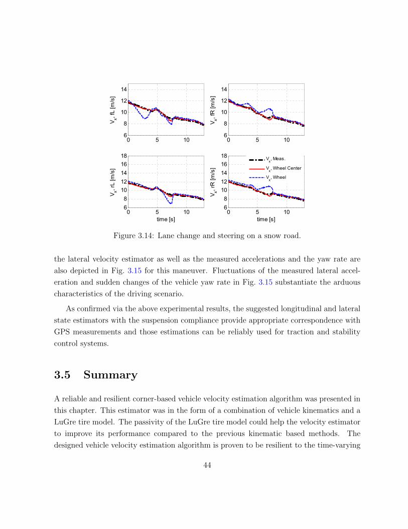
0 5 106

8

10

12

14

V x, fL

[m/s

]

0 5 106

8

10

12

14

V x, fR

[m/s

]0 5 10

68

1012141618

V x, rL

[m/s

]

time [s]0 5 10

68

1012141618

V x, rR

[m/s

]time [s]

Vx, Meas.

Vx, Wheel Center

Vx, Wheel

4WD, LC and steering on snow_20140820_test032

Figure 3.14: Lane change and steering on a snow road.

the lateral velocity estimator as well as the measured accelerations and the yaw rate are

also depicted in Fig. 3.15 for this maneuver. Fluctuations of the measured lateral accel-

eration and sudden changes of the vehicle yaw rate in Fig. 3.15 substantiate the arduous

characteristics of the driving scenario.

As confirmed via the above experimental results, the suggested longitudinal and lateral

state estimators with the suspension compliance provide appropriate correspondence with

GPS measurements and those estimations can be reliably used for traction and stability

control systems.

3.5 Summary

A reliable and resilient corner-based vehicle velocity estimation algorithm was presented in

this chapter. This estimator was in the form of a combination of vehicle kinematics and a

LuGre tire model. The passivity of the LuGre tire model could help the velocity estimator

to improve its performance compared to the previous kinematic based methods. The

designed vehicle velocity estimation algorithm is proven to be resilient to the time-varying

44

4WD, LC and steering on snow_20140820_test032

0 2 4 6 8 10 12-3

-2

-1

0

1

V y at C

G [m

/s]

time [s]

Vy,Meas.

Vy,Est. with SC

0 5 10

-2

0

2

4

6

Acc

eler

atio

ns [m

/s2 ]

time [s]

Long. ax

Lat. ay

0 5 10-0.5

0

0.5

Yaw

rate

, r [r

ad/s

]time [s]

Figure 3.15: Lateral velocity estimates for a lane change (LC) on a snow road.

tire parameters, the road friction condition, as well as sensor measurements uncertainties.

The observability of the dynamics as a linear time-varying system, due to the time-varying

wheel speed, was analytically studied prior to designing the observer. In order to further

increase the performance of the designed velocity estimation algorithm, the effect of the

suspension compliance and the resulting extra degree of freedom was directly added to the

estimated vehicle corner velocity. The performance of the proposed velocity estimation

algorithm was verified via several experimental tests, which were comprised of various

standard vehicle maneuvers performed on different road conditions, and the results showed

appropriate correspondence with measurements.

45

Chapter 4

Reliability of the Vehicle Corner

Velocity Estimation

In the previous chapter, a corner-based vehicle velocity estimation algorithm was intro-

duced in the form of a combination of vehicle kinematic relations and LuGre tire model.

Moreover, the effect of the suspension compliance on the accuracy of the resulting esti-

mator was discussed. Furthermore, several experimental results validated the performance

of the designed velocity estimator. In this chapter, a closer look is taken to the proposed

velocity estimator. In particular, using system-theoretic concepts and techniques, rigorous

stability, performance, and robustness analyses of the proposed velocity estimator to un-

certainties and external disturbances is performed. The performance metrics that will be

introduced for the velocity estimator can be considered as fundamental limitations that

one can expect from the estimator to meet in terms of performance and resilience to un-

certainties. Because of that, this chapter’s analysis is referred to as the off-line reliability

analysis of the vehicle velocity estimation [70]. An on-line approach to the estiamtor’s

reliability analysis will be discussed in the subsequent chapter.

46

4.1 Estimator’s Stability, Robustness and Sensitivity

Analysis

The stability and resilience of the vehicle velocity estimator is investigated in this section.

More particularly, the stability of the observer error dynamics (3.9) and (3.15) is analyzed

as a linear time-varying system. Moreover, the robustness of the observer dynamics to

model uncertainties will be investigated, and the sensitivity of the stability margin and

H∞ robustness of the error dynamics (3.9) and (3.15) to sensor measurements noises and

road condition uncertainties will be discussed.

4.1.1 Stability and H∞ Performance

The following proposition introduces a bound on the estimation error in (3.9) and (3.15).

A conventional approach is to study the stability of the symmetric part of the matrices

Aex and Aey , which usually results in conservative results [76]. In order to tackle such

conservativeness, a similarity transformation is utilized in the following proposition to

show the boundedness of the estimation error.

Proposition 1 Estimation errors in linear time-varying error dynamics (3.9) and (3.15)

are bounded.

Proof 1 A similarity transformation in the form of eq(t) = Teq(t), where q ∈ x, y, is

employed on the longitudinal/lateral estimation error states (3.9) and (3.15), which results

in Aeq = TAeqT−1 and Beq = TBeq . Choosing T = diag(γ, 1) with a design parameter

γ > 0, leads to Aeq whose stability margin, SMq , maxiλi(Aeq), is close to the stability

margin of its symmetric part (which will be discussed in Example 1 later). Moreover, due

to the fact that ||T|| and ||T−1|| are bounded, the transformation matrix T preserves the

exponential stability and the exponent (rate) of the convergence [77, 78]. The Lyapunov

candidate V(eq(t)) = 12eq(t)

T eq(t) is then introduced to investigate the stability of the error

dynamics (3.9) and (3.15)1. The time derivative of the Lyapunov function along the state

1V(eq(t)) and V are used interchangeably.

47

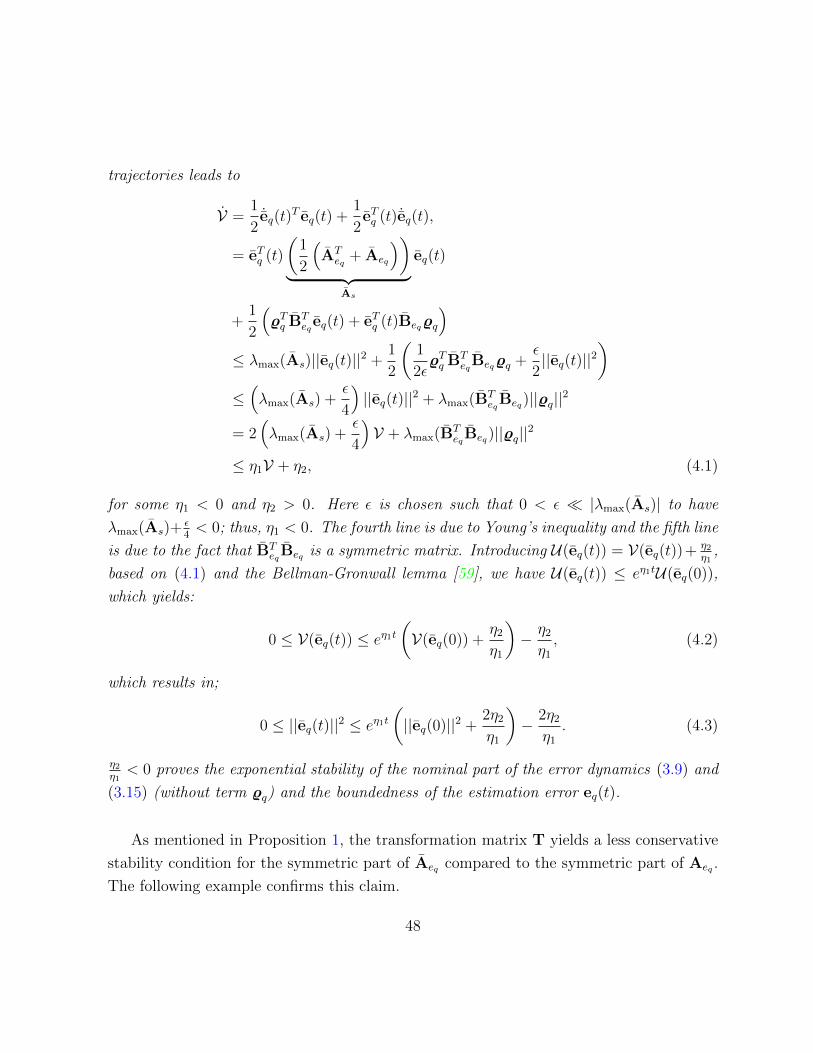
trajectories leads to

V =1

2˙eq(t)

T eq(t) +1

2eTq (t) ˙eq(t),

= eTq (t)

(1

2

(ATeq + Aeq

))︸ ︷︷ ︸

As

eq(t)

+1

2

(%Tq BT

eq eq(t) + eTq (t)Beq%q

)≤ λmax(As)||eq(t)||2 +

1

2

(1

2ε%Tq BT

eqBeq%q +ε

2||eq(t)||2

)≤(λmax(As) +

ε

4

)||eq(t)||2 + λmax(BT

eqBeq)||%q||2

= 2(λmax(As) +

ε

4

)V + λmax(BT

eqBeq)||%q||2

≤ η1V + η2, (4.1)

for some η1 < 0 and η2 > 0. Here ε is chosen such that 0 < ε |λmax(As)| to have

λmax(As)+ε4< 0; thus, η1 < 0. The fourth line is due to Young’s inequality and the fifth line

is due to the fact that BTeqBeq is a symmetric matrix. Introducing U(eq(t)) = V(eq(t))+ η2

η1,

based on (4.1) and the Bellman-Gronwall lemma [59], we have U(eq(t)) ≤ eη1tU(eq(0)),

which yields:

0 ≤ V(eq(t)) ≤ eη1t(V(eq(0)) +

η2

η1

)− η2

η1

, (4.2)

which results in;

0 ≤ ||eq(t)||2 ≤ eη1t(||eq(0)||2 +

2η2

η1

)− 2η2

η1

. (4.3)

η2η1< 0 proves the exponential stability of the nominal part of the error dynamics (3.9) and

(3.15) (without term %q) and the boundedness of the estimation error eq(t).

As mentioned in Proposition 1, the transformation matrix T yields a less conservative

stability condition for the symmetric part of Aeq compared to the symmetric part of Aeq .

The following example confirms this claim.

48

Example 1 Consider error dynamics (3.9) with the observer gains Lx = [1.18, 387]T .

For a particular angular velocity, e.g. ω = 40, the largest eigenvalue of matrix Aex and its

symmetric parts are λmax(Aex) = −327.1 and λmax(0.5(Aex+ATex)) = 108750, respectively.

Thus, the symmetric part is unstable while matrix Aex is Hurwitz. However if we use the

similarity transformation mentioned in Proposition 1 with T = diag(9000, 1), the largest

eigenvalue of the symmetric part of Aex is λmax(As) = −326.8, which is very close to

λmax(Aex). This shows how much the stability of the symmetric part of a matrix can be

conservative and how much an appropriate choice of a similarity transformation can help

in overcoming this conservativeness.

Proposition 1 shows the boundedness of the estimation errors. The tightness of this

bound is directly related to the magnitude of η2η1

as it can be concluded from (4.3). More-

over, the magnitude of this function, and in particular, η2, depends on the magnitude of

the uncertainty %q. This parameter is a function of the (unknown) road friction. If the

value of the road friction is known, the term −σ0q |Vrq |θg(Vrq)

zq which is a stabilizing term in the

LuGre model (and hence in the observer) would make the observer stability condition less

conservative.

In order to come up with some bounds on the performance of the proposed observer

from the input-output approach, system H∞ norm of error dynamics (3.9) and (3.15)

defined as H∞ , supω∈R||G(jω)||∞, where G(.) is the transfer function from uncertainty %q

to error eq, and they are shown in Figure 4.1. It should be noted that the H∞ norm is a

conservative system norm and Fig. 4.1 reveals that even conservative H∞ norms of error

dynamics2 are non-expansive (||G||∞ ≤ 1) for the suggested observers.

In the following, we extend the above H∞ analysis for the case of the time-varying case,

which is to find a set of (time-varying) gains to minimize the L2 gain from the disturbances

to the estimation error.

2 We should note that the H∞ norm is attainable for the proposed estimator in certain cases.

49

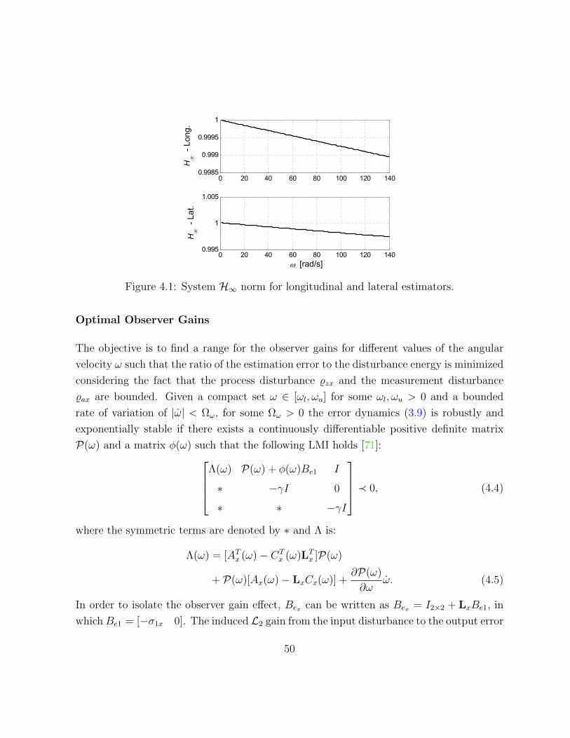
0 20 40 60 80 100 120 1400.9985

0.999

0.9995

1

H

- L

ong.

0 20 40 60 80 100 120 1400.995

1

1.005 H

-

Lat

.

[rad/s]

Figure 4.1: System H∞ norm for longitudinal and lateral estimators.

Optimal Observer Gains

The objective is to find a range for the observer gains for different values of the angular

velocity ω such that the ratio of the estimation error to the disturbance energy is minimized

considering the fact that the process disturbance %zx and the measurement disturbance

%ax are bounded. Given a compact set ω ∈ [ωl, ωu] for some ωl, ωu > 0 and a bounded

rate of variation of |ω| < Ωω, for some Ωω > 0 the error dynamics (3.9) is robustly and

exponentially stable if there exists a continuously differentiable positive definite matrix

P(ω) and a matrix φ(ω) such that the following LMI holds [71]:Λ(ω) P(ω) + φ(ω)Be1 I

∗ −γI 0

∗ ∗ −γI

≺ 0, (4.4)

where the symmetric terms are denoted by ∗ and Λ is:

Λ(ω) = [ATx (ω)− CTx (ω)LT

x ]P(ω)

+ P(ω)[Ax(ω)− LxCx(ω)] +∂P(ω)

∂ωω. (4.5)

In order to isolate the observer gain effect, Bex can be written as Bex = I2×2 + LxBe1, in

whichBe1 = [−σ1x 0]. The induced L2 gain from the input disturbance to the output error

50

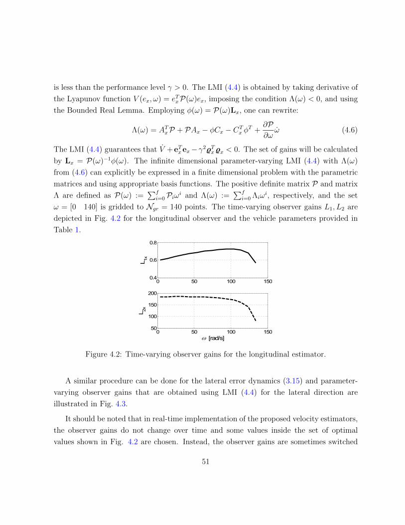
is less than the performance level γ > 0. The LMI (4.4) is obtained by taking derivative of

the Lyapunov function V (ex, ω) = eTxP(ω)ex, imposing the condition Λ(ω) < 0, and using

the Bounded Real Lemma. Employing φ(ω) = P(ω)Lx, one can rewrite:

Λ(ω) = ATxP + PAx − φCx − CTx φ

T +∂P∂ω

ω (4.6)

The LMI (4.4) guarantees that V + eTxex−γ2%Tx%x < 0. The set of gains will be calculated

by Lx = P(ω)−1φ(ω). The infinite dimensional parameter-varying LMI (4.4) with Λ(ω)

from (4.6) can explicitly be expressed in a finite dimensional problem with the parametric

matrices and using appropriate basis functions. The positive definite matrix P and matrix

Λ are defined as P(ω) :=∑f

i=0Piωi and Λ(ω) :=∑f

i=0 Λiωi, respectively, and the set

ω = [0 140] is gridded to Ngr = 140 points. The time-varying observer gains L1, L2 are

depicted in Fig. 4.2 for the longitudinal observer and the vehicle parameters provided in

Table 1.

Used for VxVy

LPV, x direction observer gains Lp1 = L1/(1+L1S1); Lp2 = L2/(1+L1S1)

0 50 100 1500.4

0.6

0.8

L 1x

0 50 100 15050

100

150

200

L 2x

[rad/s]

Figure 4.2: Time-varying observer gains for the longitudinal estimator.

A similar procedure can be done for the lateral error dynamics (3.15) and parameter-

varying observer gains that are obtained using LMI (4.4) for the lateral direction are

illustrated in Fig. 4.3.

It should be noted that in real-time implementation of the proposed velocity estimators,

the observer gains do not change over time and some values inside the set of optimal

values shown in Fig. 4.2 are chosen. Instead, the observer gains are sometimes switched

51

Used for VxVy

LPV, y direction observer gains Lp1 = L1/(1+L1S1); Lp2 = L2/(1+L1S1)

0 50 100 1500.8

1

1.2

L 1y

0 50 100 1505

10

15

20

L 2y

[rad/s]

Figure 4.3: Time-varying observer gains for the lateral estimator.

between different values in order to change the reliance of the observer to the tire force

measurements. The performance of the velocity estimator in the presence of switching

observer gains will be discussed in next section.

4.1.2 Sensitivity of the Stability Margin and H∞ Performance to

Tire Parameters

Lastly, the sensitivity of the error dynamics stability margin SMq , maxi λi(Aeq) and

system H∞ norms to model parameter uncertainties is investigated. Figs. 4.4 and 4.5

show the deviation of the stability margin of the error dynamics (3.9) and (3.15) from

their nominal values due to model parameter deviation of up to 20%.3 Fig. 4.6 shows the

sensitivity of the system H∞ norm of the error dynamics to the same parameter variations.

This figure shows that the performance of the observer is not very sensitive to the tire

parameter variations.

3Each model parameter X is perturbed as X ± 0.2X .

52

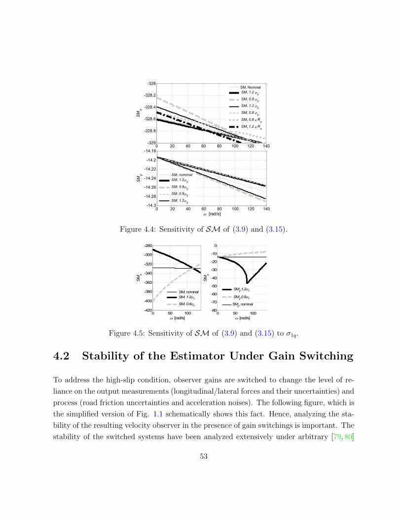
0 20 40 60 80 100 120 140-329

-328.8

-328.6

-328.4

-328.2

-328

SM

x

SM, Nominal SM, 1.2 0

SM, 0.8 0

SM, 1.2 2

SM, 0.8 2

SM, 0.8 Re

SM, 1.2 Re

0 20 40 60 80 100 120 140-14.3

-14.28

-14.26

-14.24

-14.22

-14.2

-14.18

[rad/s]

SM

y

SM, nominal SM, 1.20

SM, 0.80

SM, 0.82

SM, 1.22

Used for VxVy_suspFigure 4.4: Sensitivity of SM of (3.9) and (3.15).

Used for VxVy_susp

0 50 100-80

-70

-60

-50

-40

-30

-20

-10

0

[rad/s]

SM

y

SMy,1.21

SMy,0.81

SMy, nominal

0 50 100-420

-400

-380

-360

-340

-320

-300

-280

[rad/s]

SM

x

SM, nominal SM, 1.21

SM, 0.81

Figure 4.5: Sensitivity of SM of (3.9) and (3.15) to σ1q.

4.2 Stability of the Estimator Under Gain Switching

To address the high-slip condition, observer gains are switched to change the level of re-

liance on the output measurements (longitudinal/lateral forces and their uncertainties) and

process (road friction uncertainties and acceleration noises). The following figure, which is

the simplified version of Fig. 1.1 schematically shows this fact. Hence, analyzing the sta-

bility of the resulting velocity observer in the presence of gain switchings is important. The

stability of the switched systems have been analyzed extensively under arbitrary [79, 80]

53

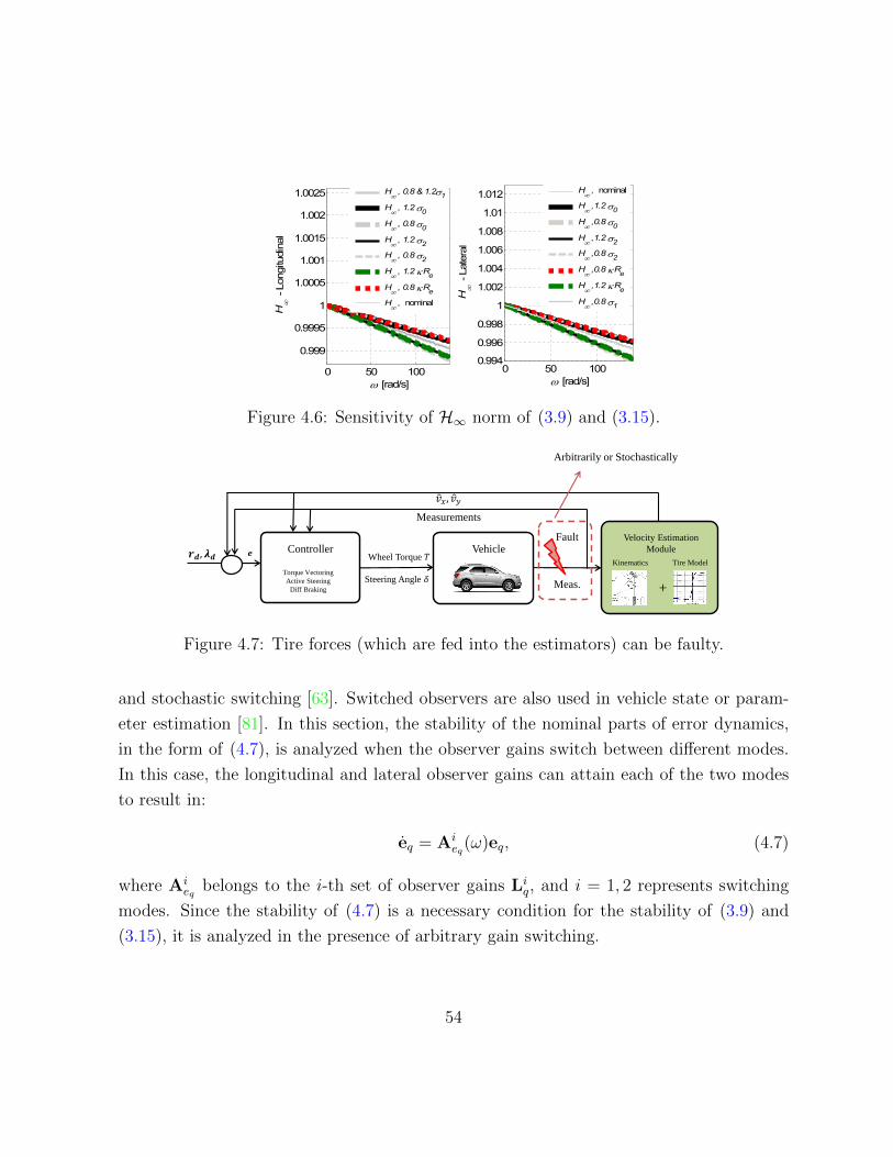
Used for VxVy_susp

0 50 1000.994

0.996

0.998

1

1.002

1.004

1.006

1.008

1.01

1.012

[rad/s]

H -

Lat

eral

H , nominal

H ,1.2 0

H ,0.8 0

H ,1.2 2

H ,0.8 2

H ,0.8 Re

H ,1.2 Re

H ,0.8 1

0 50 100

0.999

0.9995

1

1.0005

1.001

1.0015

1.002

1.0025

[rad/s]

H -

Lon

gitu

dina

l

H , 0.8 & 1.21

H , 1.2 0

H , 0.8 0

H , 1.2 2

H , 0.8 2

H , 1.2 Re

H , 0.8 Re

H , nominal

Figure 4.6: Sensitivity of H∞ norm of (3.9) and (3.15).

Measurements

𝒆

𝑣 𝑥, 𝑣 𝑦

Vehicle

Meas.

Velocity Estimation

Module

Tire Model

+

Kinematics Wheel Torque 𝑇

Steering Angle 𝛿

Controller

Torque Vectoring

Active Steering

Diff Braking

𝒓𝒅, 𝝀𝒅

Fault

Arbitrarily or Stochastically

Figure 4.7: Tire forces (which are fed into the estimators) can be faulty.

and stochastic switching [63]. Switched observers are also used in vehicle state or param-

eter estimation [81]. In this section, the stability of the nominal parts of error dynamics,

in the form of (4.7), is analyzed when the observer gains switch between different modes.

In this case, the longitudinal and lateral observer gains can attain each of the two modes

to result in:

eq = Aieq(ω)eq, (4.7)

where Aieq belongs to the i-th set of observer gains Li

q, and i = 1, 2 represents switching

modes. Since the stability of (4.7) is a necessary condition for the stability of (3.9) and

(3.15), it is analyzed in the presence of arbitrary gain switching.

54

4.2.1 Stability of the observer under arbitrarily switching gains

A sufficient condition for the quadratic stability of a switched linear system under arbitrary

switching is to have a common quadratic Lyapunov function for all switching modes [79].

Similar to the analysis done in Proposition 1, we introduce the transformed matrix Aieq =

TAieqT

−1 with the same transformation matrix T used in Proposition 1. By choosing the

Lyapunov function V(eq) = 12eTq eq, one can write:

V =1

2˙eq(t)

T eq(t) +1

2eTq (t) ˙eq(t)

= eTq (t)

(1

2

(AiT

eq + Aieq

))︸ ︷︷ ︸

Ais

eq(t) ≤ λmax(Ais)||eq||2

= 2λmax(Ais)V ≤ λV , (4.8)

where λ = maxi=1,2maxt≥02λmax(Ai

s). This shows that the decaying rate of the switched

system is based on the worst case decaying rate over time and over switching modes. This

is due to the lack of knowledge about the switching policy. In the following subsection, the

stability of the suggested observers under stochastic gain switching is analyzed, and the

results will be compared to the case of arbitrary switching.

4.2.2 Stability of the observer under stochastically switching gains

In this subsection, switching between the observer gains is assumed to happen in the

form of a particular stochastic process represented by a Markov chain. The stability of

the Markov jump linear systems has been analyzed in depth [63], [69], [64]. Similar to

the arbitrary switching case mentioned in the previous section, stochastic switching will

introduce dynamics that is comprised of two sub-dynamics4. The switching mechanism is

4Since the switching forms a Markov jump linear system and theoretical results (e.g. Theorem 1) for

such systems are derived for discrete time case, the discrete version of the estimator with the sampling

time T = 5ms is used in the experiment setup.

55

modeled using a Markov chain with the probability transition matrix:

P =

p11 p12

p21 p22

, (4.9)

where pij = Pr(L[k + 1] = Ljq|L[k] = Li

q). Here, L is a random vector that takes its

values from the sample space S = L1q,L

2q, which are the two sets of observer gains. The

following definition is required to investigate the stability of such a switched system.

Definition 1 [68] The linear system eq[k + 1] = Adieqeq[k] (matrix Adi

eq is the discrete

version of Aieq in the error dynamics (4.7), as discussed in Remark 2) is called mean

square stable (MSS) if limk→∞ E(eq[k]Teq[k]) = 0.

Based on Definition 1, the following theorem is used for the mean square stability of

the error dynamics.

Theorem 1 [82] The linear system eq[k+1] = Adieqeq[k] is MSS if and only if the following

condition holds.

ρ[(PT ⊗ I)diag(Adi

eq ⊗Adieq)]< 1, (4.10)

where ⊗ is the matrix Kronecker product, P is the probability transition matrix between

different modes and ρ[.] is the spectral radius of a matrix.

The spectral radius result provides a necessary and sufficient condition for stability under

Markovian jumps as well as a measure for the robustness of such stability. In this direction,

the stability margin of the linear Markov jump system is given by 1− ρ. In the following

example, the stability margin of the observer when the observer gains are switching with

a pre-specified Markovian jump policy is discussed, and it is shown how that stochastic

switching policy between the observer gains provides tighter results when compared to the

arbitrary switching.

Example 2 Given two high-slip and low-slip cases with the slip ratio λ = Re|ω|−VxtmaxRe|ω|,Vxt and

subsequent switching actions, a probability transition matrix represents switching policies

56

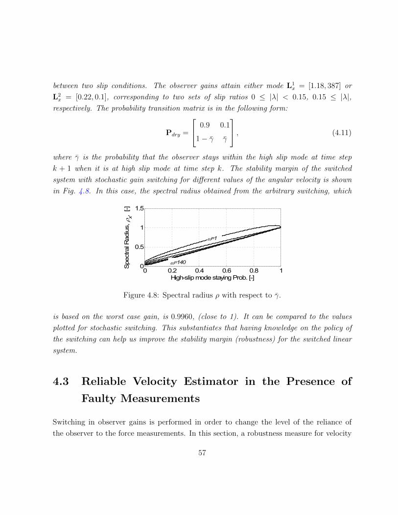
between two slip conditions. The observer gains attain either mode L1x = [1.18, 387] or

L2x = [0.22, 0.1], corresponding to two sets of slip ratios 0 ≤ |λ| < 0.15, 0.15 ≤ |λ|,

respectively. The probability transition matrix is in the following form:

Pdry =

0.9 0.1

1− γ γ

, (4.11)

where γ is the probability that the observer stays within the high slip mode at time step

k + 1 when it is at high slip mode at time step k. The stability margin of the switched

system with stochastic gain switching for different values of the angular velocity is shown

in Fig. 4.8. In this case, the spectral radius obtained from the arbitrary switching, which

Used for VxVy_susp

0 0.2 0.4 0.6 0.8 10

0.5

1

1.5

Spe

ctra

l Rad

ius,

x,

[-]

High-slip mode staying Prob. [-]

=140

=1

Figure 4.8: Spectral radius ρ with respect to γ.

is based on the worst case gain, is 0.9960, (close to 1). It can be compared to the values

plotted for stochastic switching. This substantiates that having knowledge on the policy of

the switching can help us improve the stability margin (robustness) for the switched linear

system.

4.3 Reliable Velocity Estimator in the Presence of

Faulty Measurements

Switching in observer gains is performed in order to change the level of the reliance of

the observer to the force measurements. In this section, a robustness measure for velocity

57

observers to the force measurement (estimation) failure, which acts in a cascading scheme,

is proposed. Taking advantage of the newly proposed stochastic approach in the previous

section, a metric (namely pcr) is introduced that represents the robustness of the velocity

observer to the unreliable force estimation.

Suppose that the measurement signal is faulty and does not reach the observer correctly

with some probability p, so it can not be utilized (it is dropped) by the longitudinal/lateral

observers. It is equivalent to the condition where the observer gain is Lq = 0 with proba-

bility p and nonzero (active observer gain Lq) with probability 1− p. More formally:

eq[k + 1] =

Adqeq[k] with probability p

Adeqeq[k] with probability 1− p

. (4.12)

Recasting this problem into a Markovian jump analysis, one can express the probability

transition matrix as:

P =

1− p p

1− p p

, (4.13)

with pij = Pr(L[k + 1] = Ljq|L[k] = Li

q) in which L is a random vector that takes values

from the sample space S = Lq,0. Applying Theorem 1, one can specify how tolerant

the velocity observers are against faulty force measurements. This leads to the calculation

of pcr (namely critical probability), which is defined as the maximum allowable probability

of faulty measurements occurring such that the velocity observer remains MSS.

Remark 5 In the case of measurement drop with p < pcr, the system is no longer ob-

servable. However, since the unobservable modes are MSS, the system is stochastically

detectable [83]. Figure 4.9 illustrates the value of the critical probability pcr for different

values of the wheel speed for the longitudinal and lateral velocity estimators. For probabil-

ities larger than the pcr, the system is not MSS.

Figure 4.10 depicts the value of the spectral radius ρ for the longitudinal and lateral

velocity estimators and different wheel speeds. This information can provide a sense of the

stability margin of such systems [63].

58

Used for VxVy

Packet drop, Pcr vs. omega, Vx (L = 1, 350) and Vy (L = 700, 10000)

0 20 40 60 80 100 120 140

0.2

0.4

0.6

0.8

1

[rad/s]

Crit

ical

Pro

b.,

p cr [

-]

Longitudinal observerLateral observer

Figure 4.9: Critical probabilities for the velocity observers.

0 0.2 0.4 0.6 0.8 10

0.5

1

1.5Specteral Radius ρ, both direct.

Spe

ctra

l Rad

ius,

ρx, ρ

y [−

]

Longitudinal and Lateral p [−]

Longtudinal Obs.

Lateral Obs.

ω=1

ω=1

ω=140

ω=140

Figure 4.10: Spectral radius vs. failure probability for various ω.

In the following example, the stability and robustness of the system is studied in a case

where the measurement signal drops with a certain probability. The values used in Example

3 are chosen to compare the conservativeness of the stability margin of the stochastic and

arbitrary switching scenarios, and the value of p is not obtained from road experiment.

Example 3 Given the case where the measurement signal is dropped with p = 0.2 and

reaches the estimator with probability 1 − p = 0.8 (i.e. Lx = 0 with p = 0.2 and Lx =

[1.18 387]T with 1− p = 0.8), the MSS is investigated. Applying Theorem 1 in this case

leads to a mean square stable system with the spectral radius ρ = 0.9026. Alternatively, if

the measurement signal loss happens arbitrarily, based on the arbitrary switching discussed

in section 4.2, the system becomes marginally stable, i.e. ρ = 1.

Therefore, investigating the faulty measurement cases with the Markovian jump model

59

provides a less conservative criterion for the mean square stability of the estimators.

4.4 Summary

The performance and robustness of the corner-based vehicle velocity estimator, presented

in Chapter 3, were analyzed in this chapter using system theoretic tools. More specifically,

stability of the observer error dynamics, as a linear-time-varying system, was proven based

on Lyapunov analysis, and a bound on the estimation error, as a function of road condition

and measurements uncertainties, was derived. Other than this analytical bound, some

numerical upper bounds on the estimation error dynamics were presented, which were based

on an input-output approach to the observer error dynamics and their H∞ performance,

and it was shown that the observer error dynamics is a non-expansive system (i.e., it

does not propagate the disturbances to the estimation error). As a real-time observer

gain switching is inevitable in experiments, to change the reliance of the estimator to

measurements in different instances, the stability of the velocity estimator in the presence

of estimation gain switchings was also studied for two cases of arbitrary and stochastic gain

switching scenarios. At the end, the sensitivity of the performance of the designed velocity

estimator to tire parameter variations was investigated. These analyses were referred to as

an offline reliability assessment of the velocity observer in this thesis.

60

Chapter 5

On-line Reliability Measures

In the previous chapter, several criteria for assessing the performance of the vehicle corner-

based velocity estimation were investigated and introduced. Those methods were referred

to as off-line reliability measures (or metrics). It is due to the fact that those are some

measures which indicate fundamental performance limitations that the designed observer

faces and determines the boundaries that we can expect this observer to meet terms of

performance and robustness to uncertainties. In this chapter, the on-line reliability analysis

of the velocity observer is discussed. As it can be inferred from its name, unlike the offline

case, this method can be implemented in real-time to assess the performance of the designed

observer.

The on-line reliability here refers to a level of confidence that one can assign to the

estimated velocities in the existence of potential uncertainties, such as uncertainties in

road condition, wheel speed, tire parameters as well as imprecision in estimated tire forces.

The overall reliability module and its interactions with the vehicle measurements and the

estimation module is shown in Fig. 5.1. According to this figure, since the reliability

module should ultimately work concurrently with the estimation module, it can only use

available measurements that the estimation module uses. Considering this limitation,

proposing reliability algorithms that provide independent results from the estimation and

act as a supervisory level is a challenging task. In the on-line approach discussed in this

chapter, vehicle kinematics together with some technical considerations are used to provide

61

Vehicle Measurements

IMU + Wheel speed+ Wheel

torque + …

Vehicle Velocity

Estimation

𝑣 𝑥, 𝑣 𝑦

On-line Reliability

Measure

𝑣 𝑥, 𝑣 𝑦

Reliability

Index

𝑎𝑥, 𝑎𝑦, 𝑟 𝑎𝑥, 𝑎𝑦, 𝜔

Figure 5.1: On-line reliability measure unit.

a reliability index showing the level of confidence to the estimated state, in a quantitative

manner.

5.1 Procedure

The essence of the real time approach is to translate the estimated velocities (in both

longitudinal and lateral directions) into a quantity that can be directly measured. Then,

via vehicle kinematic relations, one can assess the correctness of the estimated quantities

in a quantitative manner. More formally, the procedure is as follows. We use the following

kinematic relations between longitudinal and lateral accelerations and longitudinal and

lateral velocities at CG

ax = vx − rvy, ay = vy + rvx, (5.1)

where ax, ay, and r are longitudinal and lateral accelerations and yaw rate, respectively,

which are measured directly from IMU. If the estimated longitudinal and lateral velocities

(vx and vy) are correct, they should satisfy (5.1). In particular, by introducing variables

ax = ˙vx + rvy and ay = ˙vy − rvx, we define the error between the estimated and measured

quantities as

ex = |ax − ax|, ey = |ay − ay|, (5.2)

and then, by using a specific norm, we reach

e = ex + ey, (5.3)

62

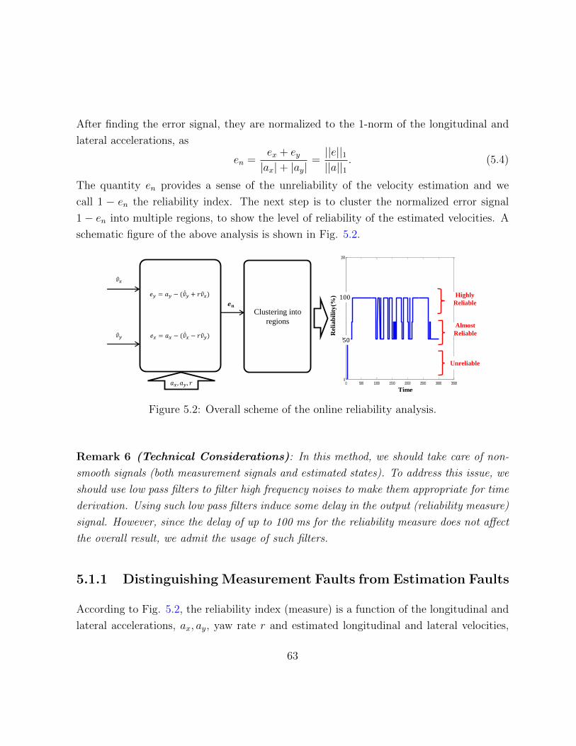
After finding the error signal, they are normalized to the 1-norm of the longitudinal and

lateral accelerations, as

en =ex + ey|ax|+ |ay|

=||e||1||a||1

. (5.4)

The quantity en provides a sense of the unreliability of the velocity estimation and we

call 1 − en the reliability index. The next step is to cluster the normalized error signal

1 − en into multiple regions, to show the level of reliability of the estimated velocities. A

schematic figure of the above analysis is shown in Fig. 5.2.

0 500 1000 1500 2000 2500 3000 35000

50

100

150

𝑣 𝑥

𝑣 𝑦

𝑎𝑥 , 𝑎𝑦 , 𝑟

𝑒𝑦 = 𝑎𝑦 − (𝑣 𝑦 + 𝑟𝑣 𝑥)

𝑒𝑥 = 𝑎𝑥 − (𝑣 𝑥 − 𝑟𝑣 𝑦)

𝒆𝒏

Clustering into

regions

Rel

iab

ilit

y(%

)

Time

Highly

Reliable

Almost

Reliable

Unreliable

100

50

Figure 5.2: Overall scheme of the online reliability analysis.

Remark 6 (Technical Considerations): In this method, we should take care of non-

smooth signals (both measurement signals and estimated states). To address this issue, we

should use low pass filters to filter high frequency noises to make them appropriate for time

derivation. Using such low pass filters induce some delay in the output (reliability measure)

signal. However, since the delay of up to 100 ms for the reliability measure does not affect

the overall result, we admit the usage of such filters.

5.1.1 Distinguishing Measurement Faults from Estimation Faults

According to Fig. 5.2, the reliability index (measure) is a function of the longitudinal and

lateral accelerations, ax, ay, yaw rate r and estimated longitudinal and lateral velocities,

63

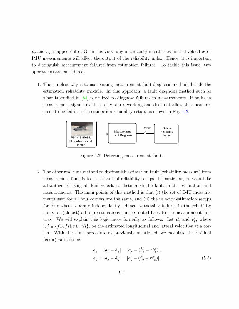
vx and vy, mapped onto CG. In this view, any uncertainty in either estimated velocities or

IMU measurements will affect the output of the reliability index. Hence, it is important

to distinguish measurement failures from estimation failures. To tackle this issue, two

approaches are considered.

1. The simplest way is to use existing measurement fault diagnosis methods beside the

estimation reliability module. In this approach, a fault diagnosis method such as

what is studied in [84] is utilized to diagnose failures in measurements. If faults in

measurement signals exist, a relay starts working and does not allow this measure-

ment to be fed into the estimation reliability setup, as shown in Fig. 5.3.

Measurement

Fault Diagnosis Vehicle meas.

IMU + wheel speed + Torque

Online Reliability

Index

𝑅𝑒𝑙𝑎𝑦

Figure 5.3: Detecting measurement fault.

2. The other real time method to distinguish estimation fault (reliability measure) from

measurement fault is to use a bank of reliability setups. In particular, one can take

advantage of using all four wheels to distinguish the fault in the estimation and

measurements. The main points of this method is that (i) the set of IMU measure-

ments used for all four corners are the same, and (ii) the velocity estimation setups

for four wheels operate independently. Hence, witnessing failures in the reliability

index for (almost) all four estimations can be rooted back to the measurement fail-

ures. We will explain this logic more formally as follows. Let vix and viy, where

i, j ∈ fL, fR, rL, rR, be the estimated longitudinal and lateral velocities at a cor-

ner. With the same procedure as previously mentioned, we calculate the residual

(error) variables as

eix = |ax − aix| = |ax − ( ˙vix − rviy)|,eiy = |ay − aiy| = |ay − ( ˙viy + rvix)|, (5.5)

64

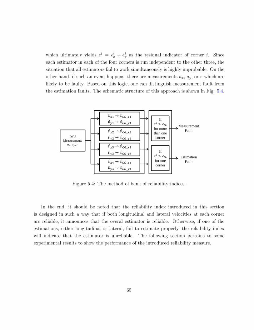
which ultimately yields ei = eix + eiy as the residual indicator of corner i. Since

each estimator in each of the four corners is run independent to the other three, the

situation that all estimators fail to work simultaneously is highly improbable. On the

other hand, if such an event happens, there are measurements ax, ay, or r which are

likely to be faulty. Based on this logic, one can distinguish measurement fault from

the estimation faults. The schematic structure of this approach is shown in Fig. 5.4.

IMU

Measurements

𝑎𝑥, 𝑎𝑦, 𝑟

𝑣 𝑥1 → 𝑣 𝐶𝐺_𝑥1

𝑣 𝑦1 → 𝑣 𝐶𝐺_𝑦1

𝑣 𝑥2 → 𝑣 𝐶𝐺_𝑥2

𝑣 𝑦2 → 𝑣 𝐶𝐺_𝑦2

𝑣 𝑥3 → 𝑣 𝐶𝐺_𝑥3

𝑣 𝑦3 → 𝑣 𝐶𝐺_𝑦3

𝑣 𝑥4 → 𝑣 𝐶𝐺_𝑥4

𝑣 𝑦4 → 𝑣 𝐶𝐺_𝑦4

If

𝑒𝑖 > 𝑒𝑡ℎ

for more

than one

corner

Measurement

Fault

If

𝑒𝑖 > 𝑒𝑡ℎ

for one

corner

Estimation

Fault

Figure 5.4: The method of bank of reliability indices.

In the end, it should be noted that the reliability index introduced in this section

is designed in such a way that if both longitudinal and lateral velocities at each corner

are reliable, it announces that the overal estimator is reliable. Otherwise, if one of the

estimations, either longitudinal or lateral, fail to estimate properly, the reliability index

will indicate that the estimator is unreliable. The following section pertains to some

experimental results to show the performance of the introduced reliability measure.

65

5.2 Applying Reliability Indices to Modify the Esti-

mated Velocities

In the previous section, a reliability measure for the estimated velocities at each corner

was proposed. This measure can be used as an indicator to inform the control module how

much it can rely on the estimated velocities. However, the estimation module itself can

also take advantage of the reliability measure [85–87]. The procedure of applying such a

reliability measure in enhancing the estimation is the subject of this section. Before that,

some required definitions are introduced.

5.2.1 Some network definitions

An undirected graph (network) is denoted by G = V , E, where V = v1, v2, . . . , vn is a

set of nodes (or vertices) and E ⊂ V × V is the set of edges. Neighbors of node vp ∈ V are

given by the set Np = vj ∈ V | (vp, vj) ∈ E. The adjacency matrix of the graph is given

by a symmetric and binary n×n matrix A, where element Apj = 1 if (vp, vj) ∈ E and zero

otherwise. The degree of node vp is denoted by dp =∑n

j=1Apj. The Laplacian matrix of

the graph is given by L = D − A, where D = diagd1 , d2 , . . . , dn.

5.2.2 Opinion Dynamics for Reliable Vehicle Estimation

The procedure of modifying the estimated corner velocities via applying the reliability

measures is now introduced. The estimated velocity of each corner, denoted by Vi(t), where

i ∈ fL, fR, rL, rR, is mapped into CG. The mapped value of each corner is called the

opinion of that corner and is denoted by ψi(t). In addition to this opinion, a confidence level

is assigned to each corner, which is determined by the online reliability measure, mentioned

in the previous section. A more reliable corner receives a larger confidence level regarding

its estimated velocity. The confidence level of corner i to opinion ψi is denoted by κi > 0,

as shown in Fig. 5.5. In an ideal case, all mapped velocities to CG should reach a unique

value, which is the velocity of the vehicle in CG. However, this does not happen in reality

66

𝑉 𝑓𝑅

𝑉 𝑓𝐿 𝑉 𝑟𝐿

𝑉 𝑟𝑅 (𝜓𝑟𝑅 , 𝜅𝑟𝑅) (𝜓𝑓𝑅 , 𝜅𝑓𝑅)

(𝜓𝑟𝐿 , 𝜅𝑟𝐿) (𝜓𝑓𝐿 , 𝜅𝑓𝐿)

𝐶𝐺

Figure 5.5: Corner opinions and their confidence level.

and there are four different values (opinions) in CG. The reason of mapping all velocities

into CG is to introduce an opinion dynamics that converges to a unique equilibrium point

closer to the estimated corner velocity with the highest confidence level. More formally,

the proposed dynamics for each opinion is in the following form [88,89]

ψk(t) =∑j∈Nk

(ψk(t)− ψj(t))− κj(ψk(t)− ψk(0)). (5.6)

Aggregating the states of all opinions into a vector ψ(t) ∈ R4, equation (5.6) yields the

following opinion dynamics for longitudinal or lateral directions

ψ(t) = −Lψ(t) + Kψ(0),

y(t) = ψ(t), (5.7)

in which y(t) is the output of interest, L = L + K where L is the Laplacian matrix 1,

and confidence matrix K = diagκfL, κfR, κrL, κrR indicates the level of confidence of the

corners. Since each corner can communicate with other three ones, the communication

graph for each direction i is a complete graph and we have

L =

3 + κfL −1 −1 −1

−1 3 + κfR −1 −1

−1 −1 3 + κrL −1

−1 −1 −1 3 + κrR

. (5.8)

1Since K is a positive definite matrix, we can easily verify that L is also a positive definite matrix.

67

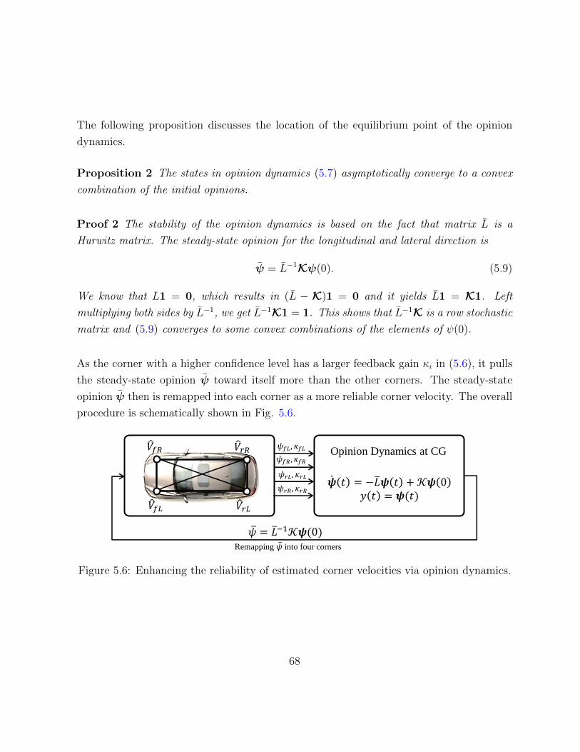
The following proposition discusses the location of the equilibrium point of the opinion

dynamics.

Proposition 2 The states in opinion dynamics (5.7) asymptotically converge to a convex

combination of the initial opinions.

Proof 2 The stability of the opinion dynamics is based on the fact that matrix L is a

Hurwitz matrix. The steady-state opinion for the longitudinal and lateral direction is

ψ = L−1Kψ(0). (5.9)

We know that L1 = 0, which results in (L − K)1 = 0 and it yields L1 = K1. Left

multiplying both sides by L−1, we get L−1K1 = 1. This shows that L−1K is a row stochastic

matrix and (5.9) converges to some convex combinations of the elements of ψ(0).

As the corner with a higher confidence level has a larger feedback gain κi in (5.6), it pulls

the steady-state opinion ψ toward itself more than the other corners. The steady-state

opinion ψ then is remapped into each corner as a more reliable corner velocity. The overall

procedure is schematically shown in Fig. 5.6.

𝜓𝑟𝐿, 𝜅𝑟𝐿

𝜓𝑓𝐿, 𝜅𝑓𝐿

𝜓𝑓𝑅 , 𝜅𝑓𝑅

𝜓𝑟𝑅 , 𝜅𝑟𝑅

𝑉 𝑓𝑅

𝑉 𝑓𝐿 𝑉 𝑟𝐿

𝑉 𝑟𝑅 Opinion Dynamics at CG

𝜓 = 𝐿 −1𝒦𝝍(0)

𝝍 𝑡 = −𝐿 𝝍 𝑡 + 𝒦𝝍 0

𝑦 𝑡 = 𝝍(𝑡)

Remapping 𝜓 into four corners

Figure 5.6: Enhancing the reliability of estimated corner velocities via opinion dynamics.

68

5.3 Experimental Results

In this section, some experimental results about the on-line reliability measure for the

vehicle velocity estimation for different maneuvers and on various road conditions are

demonstrated. In some of the tests, some additional fault is injected intentionally to the

estimated values at some particular time instances (or periods) to show the performance

of the on-line reliability measure. Vehicle motion characteristics are discussed and plotted

for each maneuver. In the following subsection, a simple longitudinal acceleration and

deceleration maneuver on a dry road is presented and will be followed by more complicated

maneuvers on different road conditions, discussed subsequently. It should be noted that an

experimental result showing the performance of the opinion dynamics method in enhancing

the reliability of the corner velocities was demonstrated in the previous chapter. More

specifically, the split µ longitudinal maneuver whose estimated velocities are shown in

Fig. 3.8, uses the opinion dynamics algorithm inside its estimation module to enhance the

reliability of its estimated velocity.

5.3.1 Acceleration-Deceleration on Dry Road

Here, the reliability measure (index) of the velocity estimation in a traction and brake

maneuver for a four wheel drive equinox on a dry road is demonstrated. The values of

longitudinal and lateral accelerations together with the steering angle are plotted in Fig.

5.7. The magnitudes of lateral acceleration ay and steering angle δ show that the vehicle is

fairly following a straight line. Moreover, the estimated longitudinal and lateral velocities

as dashed lines along with the GPS measurement of these velocities as solid black lines are

demonstrated. The reliability index is also depicted in Fig. 5.8.

As it is inferred from Figs. 5.7 and 5.8, the reliability index has an appropriate cor-

respondence to the accuracy of estimated velocities (compared to those of GPS measure-

ments). More specifically, in the time interval between t = 6s to t = 8s, as both estimated

longitudinal and lateral velocities deviate from the measured velocities, the reliability index

in that time interval drops down. However, as the maneuver is a simple acceleration-brake

maneuver, the performance of the reliability index is not apparent. Hence, in the following

69

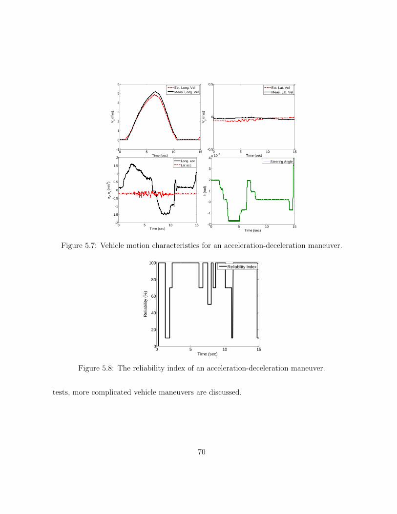
0 5 10 15-1

0

1

2

3

4

5

6

Time (sec)

Vx (

m/s

)

Est. Long. Vel

Meas. Long. Vel

0 5 10 15-0.5

0

0.5

Time (sec)

Vy (

m/s

)

Est. Lat. Vel

Meas. Lat. Vel

0 5 10 15-2

-1.5

-1

-0.5

0

0.5

1

1.5

2

Time (sec)

ax,

ay (

m/s

2)

Long. acc

Lat acc

0 5 10 15-2

-1

0

1

2

3

4x 10

-3

Time (sec)

(

rad)

Steering Angle

Figure 5.7: Vehicle motion characteristics for an acceleration-deceleration maneuver.

0 5 10 150

20

40

60

80

100

Time (sec)

Relia

bili

ty (

%)

Reliability Index

Figure 5.8: The reliability index of an acceleration-deceleration maneuver.

tests, more complicated vehicle maneuvers are discussed.

70

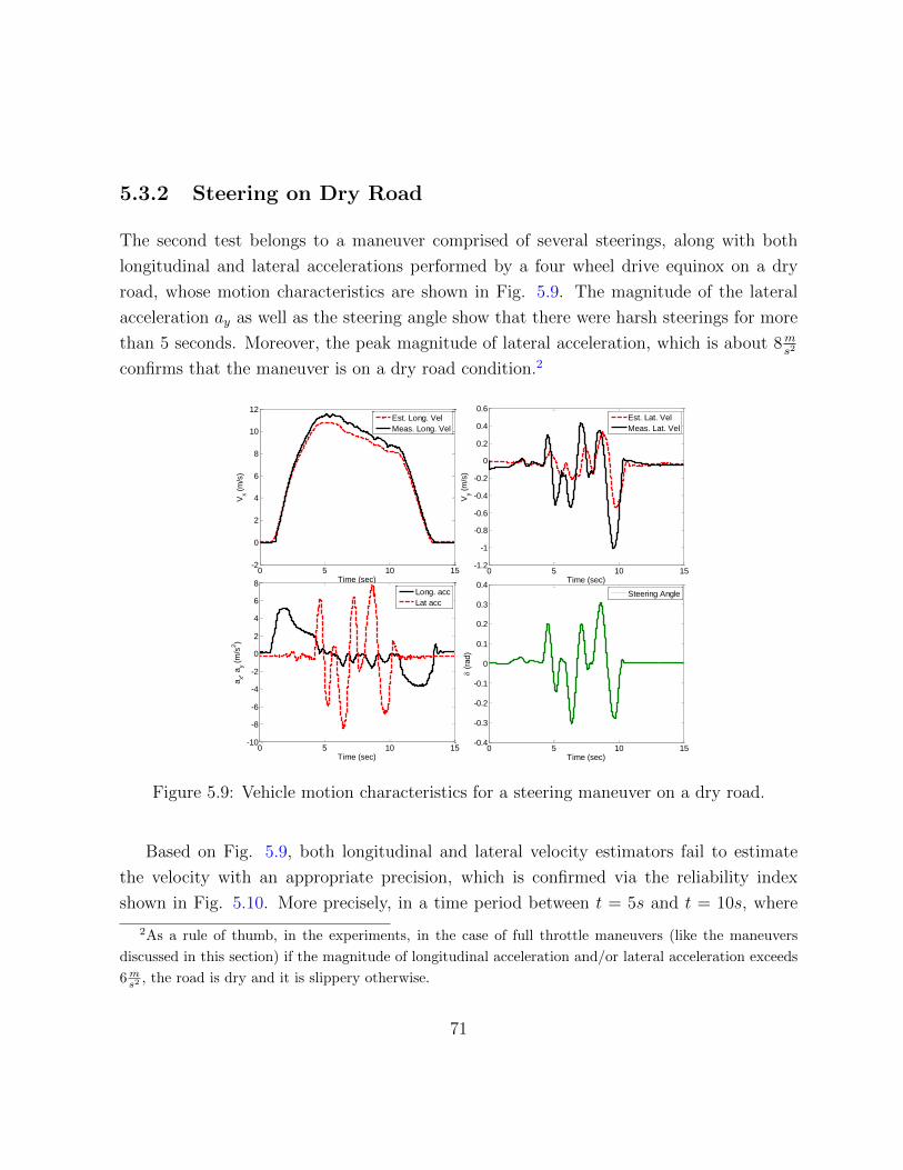
5.3.2 Steering on Dry Road

The second test belongs to a maneuver comprised of several steerings, along with both

longitudinal and lateral accelerations performed by a four wheel drive equinox on a dry

road, whose motion characteristics are shown in Fig. 5.9. The magnitude of the lateral

acceleration ay as well as the steering angle show that there were harsh steerings for more

than 5 seconds. Moreover, the peak magnitude of lateral acceleration, which is about 8ms2

confirms that the maneuver is on a dry road condition.2

0 5 10 15-2

0

2

4

6

8

10

12

Time (sec)

Vx (

m/s

)

Est. Long. Vel

Meas. Long. Vel

0 5 10 15-1.2

-1

-0.8

-0.6

-0.4

-0.2

0

0.2

0.4

0.6

Time (sec)

Vy (

m/s

)

Est. Lat. Vel

Meas. Lat. Vel

0 5 10 15-0.4

-0.3

-0.2

-0.1

0

0.1

0.2

0.3

0.4

Time (sec)

(

rad)

Steering Angle

0 5 10 15-10

-8

-6

-4

-2

0

2

4

6

8

Time (sec)

ax,

ay (

m/s

2)

Long. acc

Lat acc

Figure 5.9: Vehicle motion characteristics for a steering maneuver on a dry road.

Based on Fig. 5.9, both longitudinal and lateral velocity estimators fail to estimate

the velocity with an appropriate precision, which is confirmed via the reliability index

shown in Fig. 5.10. More precisely, in a time period between t = 5s and t = 10s, where

2As a rule of thumb, in the experiments, in the case of full throttle maneuvers (like the maneuvers

discussed in this section) if the magnitude of longitudinal acceleration and/or lateral acceleration exceeds

6ms2 , the road is dry and it is slippery otherwise.

71

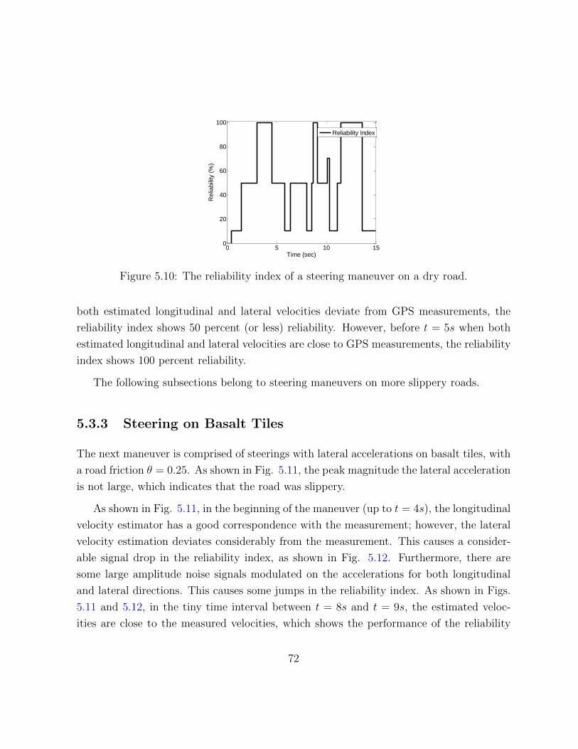
0 5 10 150

20

40

60

80

100

Time (sec)

Relia

bili

ty (

%)

Reliability Index

Figure 5.10: The reliability index of a steering maneuver on a dry road.

both estimated longitudinal and lateral velocities deviate from GPS measurements, the

reliability index shows 50 percent (or less) reliability. However, before t = 5s when both

estimated longitudinal and lateral velocities are close to GPS measurements, the reliability

index shows 100 percent reliability.

The following subsections belong to steering maneuvers on more slippery roads.

5.3.3 Steering on Basalt Tiles

The next maneuver is comprised of steerings with lateral accelerations on basalt tiles, with

a road friction θ = 0.25. As shown in Fig. 5.11, the peak magnitude the lateral acceleration

is not large, which indicates that the road was slippery.

As shown in Fig. 5.11, in the beginning of the maneuver (up to t = 4s), the longitudinal

velocity estimator has a good correspondence with the measurement; however, the lateral

velocity estimation deviates considerably from the measurement. This causes a consider-

able signal drop in the reliability index, as shown in Fig. 5.12. Furthermore, there are

some large amplitude noise signals modulated on the accelerations for both longitudinal

and lateral directions. This causes some jumps in the reliability index. As shown in Figs.

5.11 and 5.12, in the tiny time interval between t = 8s and t = 9s, the estimated veloc-

ities are close to the measured velocities, which shows the performance of the reliability

72

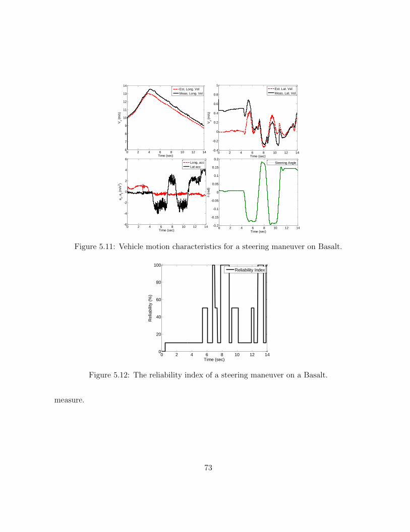
0 2 4 6 8 10 12 146

7

8

9

10

11

12

13

14

Time (sec)

Vx (

m/s

)

Est. Long. Vel

Meas. Long. Vel

0 2 4 6 8 10 12 14-0.4

-0.2

0

0.2

0.4

0.6

0.8

1

Time (sec)

Vy (

m/s

)

Est. Lat. Vel

Meas. Lat. Vel

0 2 4 6 8 10 12 14-6

-4

-2

0

2

4

6

Time (sec)

ax,

ay (

m/s

2)

Long. acc

Lat acc

0 2 4 6 8 10 12 14-0.2

-0.15

-0.1

-0.05

0

0.05

0.1

0.15

0.2

Time (sec)

(

rad)

Steering Angle

Figure 5.11: Vehicle motion characteristics for a steering maneuver on Basalt.

0 2 4 6 8 10 12 140

20

40

60

80

100

Time (sec)

Relia

bili

ty (

%)

Reliability Index

Figure 5.12: The reliability index of a steering maneuver on a Basalt.

measure.

73

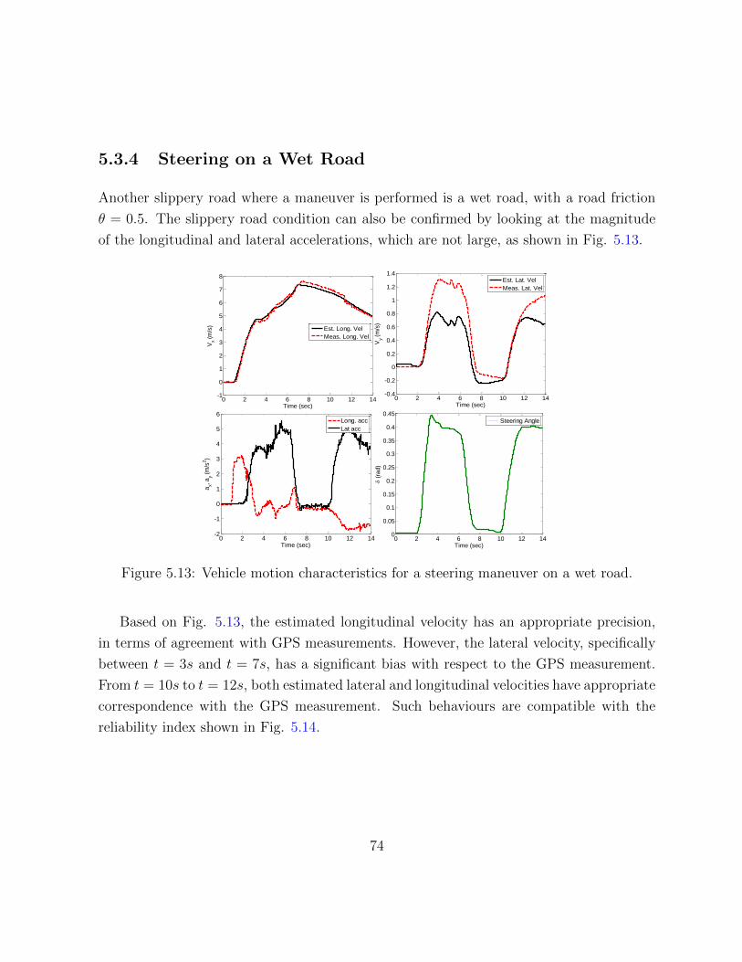
5.3.4 Steering on a Wet Road

Another slippery road where a maneuver is performed is a wet road, with a road friction

θ = 0.5. The slippery road condition can also be confirmed by looking at the magnitude

of the longitudinal and lateral accelerations, which are not large, as shown in Fig. 5.13.

0 2 4 6 8 10 12 140

0.05

0.1

0.15

0.2

0.25

0.3

0.35

0.4

0.45

Time (sec)

(

rad)

Steering Angle

0 2 4 6 8 10 12 14-2

-1

0

1

2

3

4

5

6

Time (sec)

ax,

ay (

m/s

2)

Long. acc

Lat acc

0 2 4 6 8 10 12 14-1

0

1

2

3

4

5

6

7

8

Time (sec)

Vx (

m/s

)

Est. Long. Vel

Meas. Long. Vel

0 2 4 6 8 10 12 14-0.4

-0.2

0

0.2

0.4

0.6

0.8

1

1.2

1.4

Time (sec)

Vy (

m/s

)

Est. Lat. Vel

Meas. Lat. Vel

Figure 5.13: Vehicle motion characteristics for a steering maneuver on a wet road.

Based on Fig. 5.13, the estimated longitudinal velocity has an appropriate precision,

in terms of agreement with GPS measurements. However, the lateral velocity, specifically

between t = 3s and t = 7s, has a significant bias with respect to the GPS measurement.

From t = 10s to t = 12s, both estimated lateral and longitudinal velocities have appropriate

correspondence with the GPS measurement. Such behaviours are compatible with the

reliability index shown in Fig. 5.14.

74

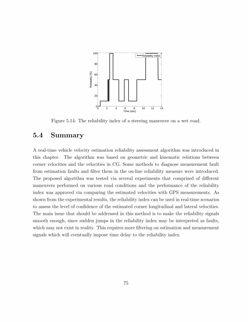
0 2 4 6 8 10 12 140

20

40

60

80

100

Time (sec)

Relia

bili

ty (

%)

Reliability Index

Figure 5.14: The reliability index of a steering maneuver on a wet road.

5.4 Summary

A real-time vehicle velocity estimation reliability assessment algorithm was introduced in

this chapter. The algorithm was based on geometric and kinematic relations between

corner velocities and the velocities in CG. Some methods to diagnose measurement fault

from estimation faults and filter them in the on-line reliability measure were introduced.

The proposed algorithm was tested via several experiments that comprised of different

maneuvers performed on various road conditions and the performance of the reliability

index was approved via comparing the estimated velocities with GPS measurements. As

shown from the experimental results, the reliability index can be used in real-time scenarios

to assess the level of confidence of the estimated corner longitudinal and lateral velocities.

The main issue that should be addressed in this method is to make the reliability signals

smooth enough, since sudden jumps in the reliability index may be interpreted as faults,

which may not exist in reality. This requires more filtering on estimation and measurement

signals which will eventually impose time delay to the reliability index.

75

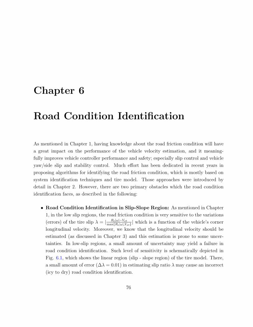
Chapter 6

Road Condition Identification

As mentioned in Chapter 1, having knowledge about the road friction condition will have

a great impact on the performance of the vehicle velocity estimation, and it meaning-

fully improves vehicle controller performance and safety; especially slip control and vehicle

yaw/side slip and stability control. Much effort has been dedicated in recent years in

proposing algorithms for identifying the road friction condition, which is mostly based on

system identification techniques and tire model. Those approaches were introduced by

detail in Chapter 2. However, there are two primary obstacles which the road condition

identification faces, as described in the following:

• Road Condition Identification in Slip-Slope Region: As mentioned in Chapter

1, in the low slip regions, the road friction condition is very sensitive to the variations

(errors) of the tire slip λ = | Re|ω|−VxtmaxRe|ω|,Vxt | which is a function of the vehicle’s corner

longitudinal velocity. Moreover, we know that the longitudinal velocity should be

estimated (as discussed in Chapter 3) and this estimation is prone to some uncer-

tainties. In low-slip regions, a small amount of uncertainty may yield a failure in

road condition identification. Such level of sensitivity is schematically depicted in

Fig. 6.1, which shows the linear region (slip - slope region) of the tire model. There,

a small amount of error (∆λ = 0.01) in estimating slip ratio λ may cause an incorrect

(icy to dry) road condition identification.

76

𝜇

𝜇0

0.03 0.04 𝜆

Dry

Wet

Figure 6.1: Sensitivity of the linear region of the tire model.

• Road Condition Identification in Low Excitation Maneuvers: A reliable

road friction identification often requires that the regression vector satisfies the per-

sistence of excitation (PE) conditions [28]. Consequently, the road friction coefficient

identification approaches mentioned in Chapter 1 demand specific vehicle maneuvers

or motion excitation (e.g., extensive steering action, accelerating and decelerating),

which could be unrealistic/impossible in certain situations/constraints, such as con-

stant speed cruising, surveillance, and military operations, and/or violate vehicle

desired motion control and trajectory tracking objectives.

According to the presented literature review on road condition identification in Chapter

2, and the concerns that this field of study faces as mentioned above, a new look to road

condition identification is proposed in this section. The approach of this study in identifying

the road condition, is to use conventional vehicle sensory measurements1 together with

the vehicle lateral dynamics, and applying some post-processing techniques to come up

with a less demanding road condition identification technique, compared to the former

methods in terms of the required richness of the actuation signal (steering and gas pedal).

Experimental tests show that the proposed method has an eminent power to address this

problem in the situations where the previous methods in the literature fail to work (i.e.

in law level of excitation and small tire slip regions). The theoretical foundation of this

1e.g., vehicle yaw rate and accelerations, wheel speed and acceleration and vehicle steering.

77

approach is discussed in the following section.

6.1 Vehicle Response-Based Road Condition Classifi-

cation

This section presents the theoretical background of the road condition identification algo-

rithm based on the vehicle response to lateral excitations. We begin by the linear lateral

dynamics described in Chapter 2. Then we extend this analysis to the nonlinear case.

6.1.1 Linear Tire Model Case

Consider the following vehicle linear bicycle model (which was discussed in Chapter 2),vy(t)r(t)

=

−Cαf+Cαr

vxm−(

aCαf−bCαrvxm

+ vx)

−aCαf−bCαrvxIz

−a2Cαf+b2Cαr

vxIz

︸ ︷︷ ︸

A

vy(t)r(t)

︸ ︷︷ ︸

x(t)

+

Cαfm

aCαfIz

︸ ︷︷ ︸

B

δ, (6.1)

where Cαf and Cαr are the cornering stiffness values for front and rear tracks, which are

functions of the road condition θ, i.e., Cαf (θ), Cαr(θ). Here vx is the longitudinal speed

obtained from a torque and road-independent approach such as [90]. Among the two

states in this dynamics, yaw rate r(t) and lateral velocity vy(t), the available measurement

is yaw rate and the lateral velocity must be estimated (as discussed in detail in Chapter 3).

Hence, here, the yaw rate r(t) is considered to be a measurable vehicle’s response and plays

a major role in the road identification algorithm. By solving (6.1) as a linear time-varying

system, one can easily find the vehicle’s yaw rate as

r(t) = [0 1]

vy(t)r(t)

= [0 1]x(t) = [0 1]

(Φ(t, t0)x(t0) +

∫ t

t0

Φ(t, τ)Bδ(τ)dτ

), (6.2)

where Φ(t, t0) is the state transition matrix. According to (6.2), the value of the vehicle

yaw rate is heavily dependent on the cornering stiffness (and hence, the road condition)

78

which appears in matrices A and B. Thus, different values of the cornering stiffness, i.e.,

different road conditions, result in different vehicle response (yaw rate). More formally, if

we consider a value for the road condition like θ (as the actual value of the road condition

is unknown), then we have

rθ(t) = [0 1]

(Φ(t, t0, θ)x(t0) +

∫ t

t0

Φ(t, τ, θ)Bθδ(τ)dτ

), (6.3)

where Φ(t, t0, θ) and Bθ are functions of the assumed value θ. By subtracting this value

from the real (measured) value of the yaw rate r(t), we get

Rr(t) = r(t)− rθ(t) = r(t)− [0 1]

(Φ(t, t0, θ)x(t0) +

∫ t

t0

Φ(t, τ, θ)Bθδ(τ)dτ

), (6.4)

where Rr(t) is the residual signal. By changing the value of θ from 0 (corresponding to the

icy road) to 1 (corresponding to the dry road), while all of the other parameters in (6.4)

are fixed, it is expected that the residual signal becomes zero at some particular value of θ.

In particular, the real-time residual signal Rr(t) is an indicator of the difference between

the actual road condition and the assumed road condition. Mathematically speaking, the

true value of the road condition is obtained from

θ(t) = arg minθRr(t). (6.5)

One can improve this approach via using other vehicle states in combination with the yaw

rate as indicators of the vehicle’s response. To this end, other two IMU measurements,

which are the vehicle’s lateral and longitudinal accelerations ax and ay, can be used as well

in order to come up with a more reliable identification algorithm. In order to use these

two quantities, one should translate the states to longitudinal and lateral accelerations as

ax = vx − rvy and ay = vy + rvx. Here, longitudinal velocity vx is obtained from the

estimation and lateral velocity is obtained from the solution of the linear lateral dynamics

(6.1) as

vyθ(t) = [1 0]

(Φ(t, t0)x(t0) +

∫ t

t0

Φ(t, τ)Bδ(τ)dτ

). (6.6)

79

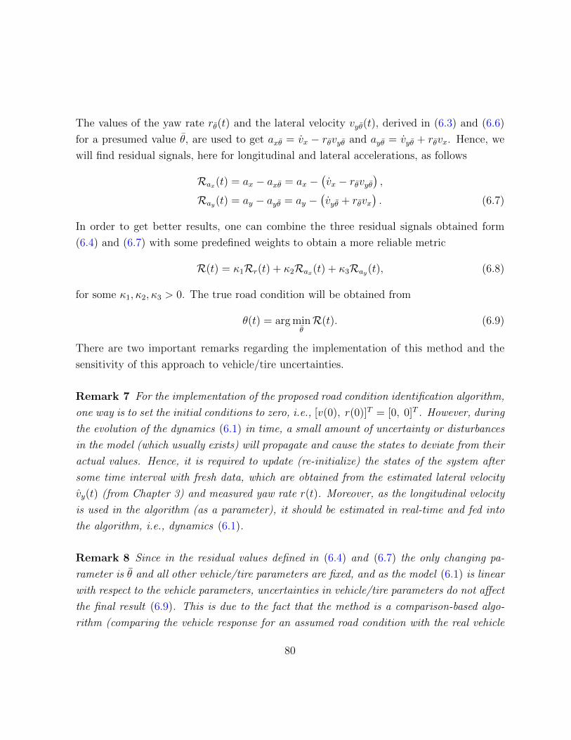
The values of the yaw rate rθ(t) and the lateral velocity vyθ(t), derived in (6.3) and (6.6)

for a presumed value θ, are used to get axθ = vx − rθvyθ and ayθ = vyθ + rθvx. Hence, we

will find residual signals, here for longitudinal and lateral accelerations, as follows

Rax(t) = ax − axθ = ax −(vx − rθvyθ

),

Ray(t) = ay − ayθ = ay −(vyθ + rθvx

). (6.7)

In order to get better results, one can combine the three residual signals obtained form

(6.4) and (6.7) with some predefined weights to obtain a more reliable metric

R(t) = κ1Rr(t) + κ2Rax(t) + κ3Ray(t), (6.8)

for some κ1, κ2, κ3 > 0. The true road condition will be obtained from

θ(t) = arg minθR(t). (6.9)

There are two important remarks regarding the implementation of this method and the

sensitivity of this approach to vehicle/tire uncertainties.

Remark 7 For the implementation of the proposed road condition identification algorithm,

one way is to set the initial conditions to zero, i.e., [v(0), r(0)]T = [0, 0]T . However, during

the evolution of the dynamics (6.1) in time, a small amount of uncertainty or disturbances

in the model (which usually exists) will propagate and cause the states to deviate from their

actual values. Hence, it is required to update (re-initialize) the states of the system after

some time interval with fresh data, which are obtained from the estimated lateral velocity

vy(t) (from Chapter 3) and measured yaw rate r(t). Moreover, as the longitudinal velocity

is used in the algorithm (as a parameter), it should be estimated in real-time and fed into

the algorithm, i.e., dynamics (6.1).

Remark 8 Since in the residual values defined in (6.4) and (6.7) the only changing pa-

rameter is θ and all other vehicle/tire parameters are fixed, and as the model (6.1) is linear

with respect to the vehicle parameters, uncertainties in vehicle/tire parameters do not affect

the final result (6.9). This is due to the fact that the method is a comparison-based algo-

rithm (comparing the vehicle response for an assumed road condition with the real vehicle

80

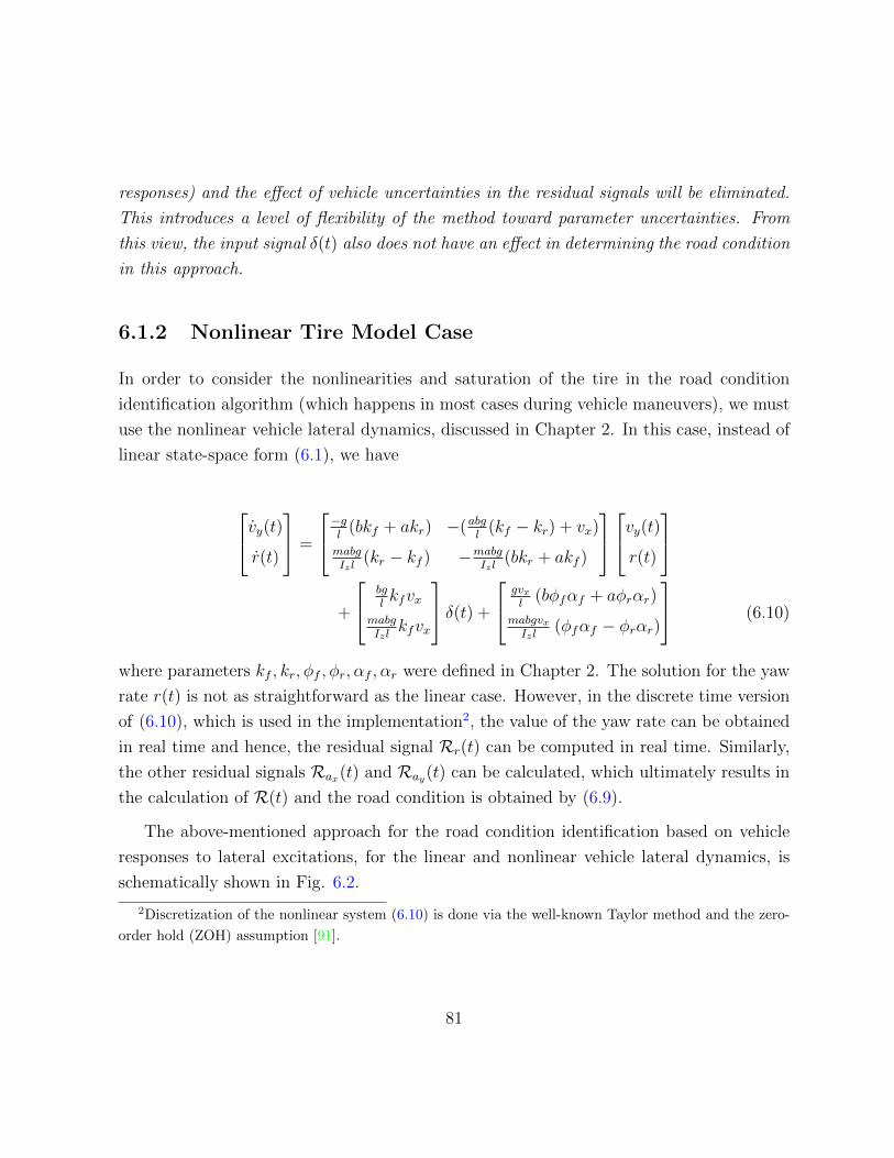
responses) and the effect of vehicle uncertainties in the residual signals will be eliminated.

This introduces a level of flexibility of the method toward parameter uncertainties. From

this view, the input signal δ(t) also does not have an effect in determining the road condition

in this approach.

6.1.2 Nonlinear Tire Model Case

In order to consider the nonlinearities and saturation of the tire in the road condition

identification algorithm (which happens in most cases during vehicle maneuvers), we must

use the nonlinear vehicle lateral dynamics, discussed in Chapter 2. In this case, instead of

linear state-space form (6.1), we have

vy(t)r(t)

=

−gl (bkf + akr) −(abgl

(kf − kr) + vx)

mabgIzl

(kr − kf ) −mabgIzl

(bkr + akf )

vy(t)r(t)

+

bglkfvx

mabgIzl

kfvx

δ(t) +

gvxl

(bφfαf + aφrαr)

mabgvxIzl

(φfαf − φrαr)

(6.10)

where parameters kf , kr, φf , φr, αf , αr were defined in Chapter 2. The solution for the yaw

rate r(t) is not as straightforward as the linear case. However, in the discrete time version

of (6.10), which is used in the implementation2, the value of the yaw rate can be obtained

in real time and hence, the residual signal Rr(t) can be computed in real time. Similarly,

the other residual signals Rax(t) and Ray(t) can be calculated, which ultimately results in

the calculation of R(t) and the road condition is obtained by (6.9).

The above-mentioned approach for the road condition identification based on vehicle

responses to lateral excitations, for the linear and nonlinear vehicle lateral dynamics, is

schematically shown in Fig. 6.2.

2Discretization of the nonlinear system (6.10) is done via the well-known Taylor method and the zero-

order hold (ZOH) assumption [91].

81

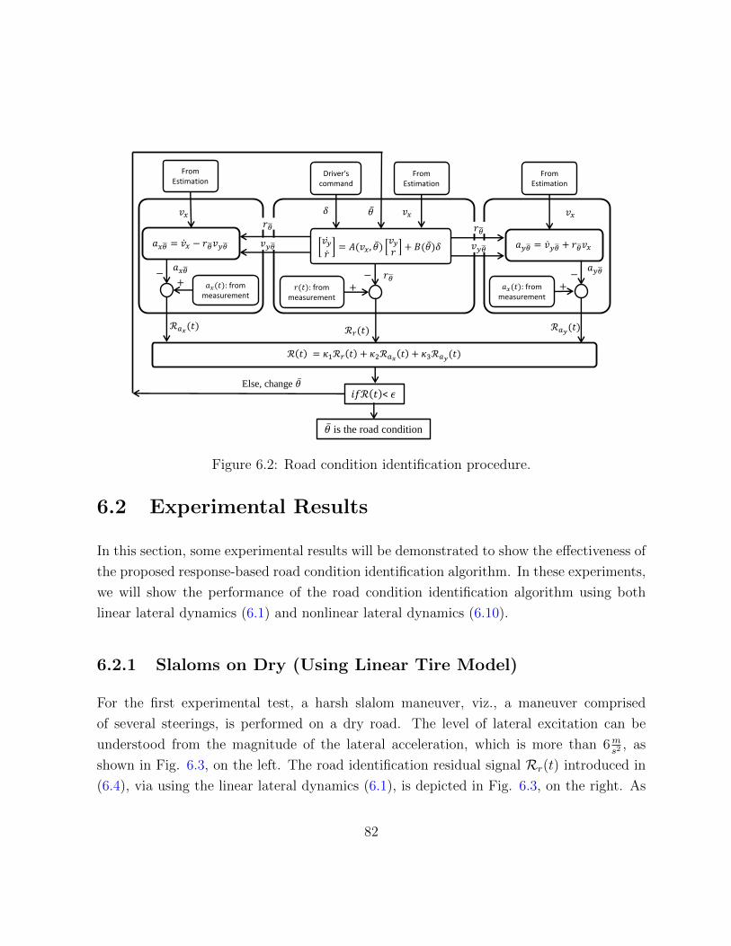
𝑣𝑦

𝑟 = 𝐴(𝑣𝑥, 𝜃 )

𝑣𝑦𝑟

+ 𝐵(𝜃 )𝛿

𝛿 𝜃 𝑣𝑥

𝑟(𝑡): from measurement

𝑟𝜃

𝑎𝑥(𝑡): from measurement

𝑣𝑦𝜃 𝑎𝑥𝜃 = 𝑣 𝑥 − 𝑟𝜃 𝑣𝑦𝜃

𝑣𝑥

+

𝑎𝑦𝜃 = 𝑣 𝑦𝜃 + 𝑟𝜃 𝑣𝑥

𝑎𝑥(𝑡): from measurement

+

+ − 𝑟𝜃

− 𝑎𝑥𝜃

− 𝑎𝑦𝜃

ℛ𝑎𝑥(𝑡) ℛ𝑟(𝑡) ℛ𝑎𝑦(𝑡)

ℛ 𝑡 = 𝜅1ℛ𝑟 𝑡 + 𝜅2ℛ𝑎𝑥 𝑡 + 𝜅3ℛ𝑎𝑦(𝑡)

𝑖𝑓ℛ 𝑡 < 𝜖

𝑣𝑥

Driver′s command

From Estimation

𝜃 is the road condition

From Estimation

From Estimation

Else, change 𝜃

𝑟𝜃

𝑣𝑦𝜃

Figure 6.2: Road condition identification procedure.

6.2 Experimental Results

In this section, some experimental results will be demonstrated to show the effectiveness of

the proposed response-based road condition identification algorithm. In these experiments,

we will show the performance of the road condition identification algorithm using both

linear lateral dynamics (6.1) and nonlinear lateral dynamics (6.10).

6.2.1 Slaloms on Dry (Using Linear Tire Model)

For the first experimental test, a harsh slalom maneuver, viz., a maneuver comprised

of several steerings, is performed on a dry road. The level of lateral excitation can be

understood from the magnitude of the lateral acceleration, which is more than 6ms2

, as

shown in Fig. 6.3, on the left. The road identification residual signal Rr(t) introduced in

(6.4), via using the linear lateral dynamics (6.1), is depicted in Fig. 6.3, on the right. As

82

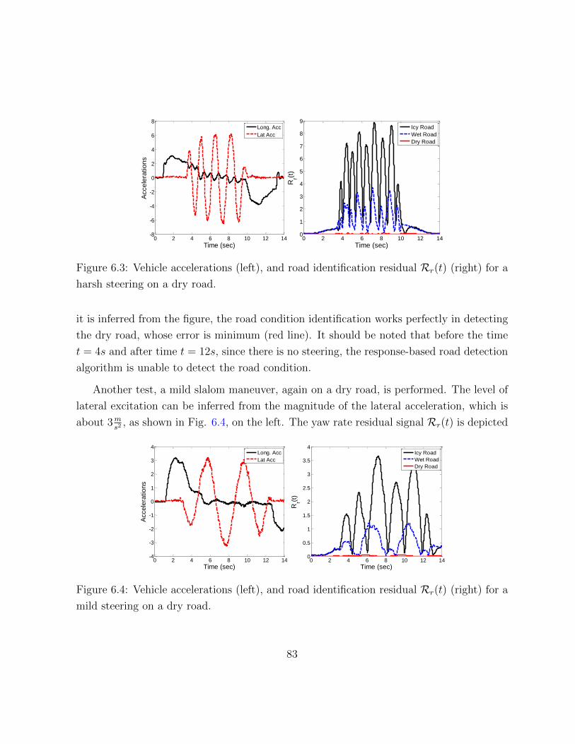
0 2 4 6 8 10 12 140

1

2

3

4

5

6

7

8

9

Time (sec)

Rr(t

)

Icy Road

Wet Road

Dry Road

0 2 4 6 8 10 12 14-8

-6

-4

-2

0

2

4

6

8

Time (sec)

Acce

lera

tio

ns

Long. Acc

Lat Acc

Figure 6.3: Vehicle accelerations (left), and road identification residual Rr(t) (right) for a

harsh steering on a dry road.

it is inferred from the figure, the road condition identification works perfectly in detecting

the dry road, whose error is minimum (red line). It should be noted that before the time

t = 4s and after time t = 12s, since there is no steering, the response-based road detection

algorithm is unable to detect the road condition.

Another test, a mild slalom maneuver, again on a dry road, is performed. The level of

lateral excitation can be inferred from the magnitude of the lateral acceleration, which is

about 3ms2

, as shown in Fig. 6.4, on the left. The yaw rate residual signal Rr(t) is depicted

0 2 4 6 8 10 12 14-4

-3

-2

-1

0

1

2

3

4

Time (sec)

Accele

rations

Long. Acc

Lat Acc

0 2 4 6 8 10 12 140

0.5

1

1.5

2

2.5

3

3.5

4

Time (sec)

Rr(t

)

Icy Road

Wet Road

Dry Road

Figure 6.4: Vehicle accelerations (left), and road identification residual Rr(t) (right) for a

mild steering on a dry road.

83

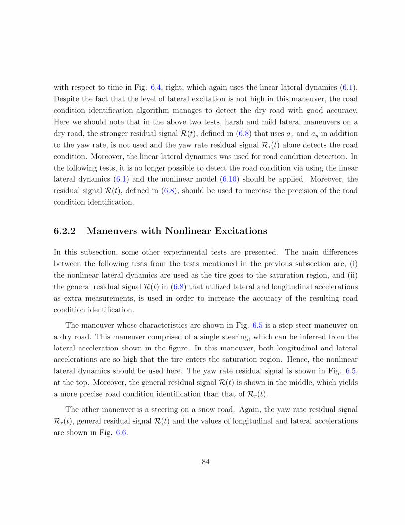
with respect to time in Fig. 6.4, right, which again uses the linear lateral dynamics (6.1).

Despite the fact that the level of lateral excitation is not high in this maneuver, the road

condition identification algorithm manages to detect the dry road with good accuracy.

Here we should note that in the above two tests, harsh and mild lateral maneuvers on a

dry road, the stronger residual signal R(t), defined in (6.8) that uses ax and ay in addition

to the yaw rate, is not used and the yaw rate residual signal Rr(t) alone detects the road

condition. Moreover, the linear lateral dynamics was used for road condition detection. In

the following tests, it is no longer possible to detect the road condition via using the linear

lateral dynamics (6.1) and the nonlinear model (6.10) should be applied. Moreover, the

residual signal R(t), defined in (6.8), should be used to increase the precision of the road

condition identification.

6.2.2 Maneuvers with Nonlinear Excitations

In this subsection, some other experimental tests are presented. The main differences

between the following tests from the tests mentioned in the previous subsection are, (i)

the nonlinear lateral dynamics are used as the tire goes to the saturation region, and (ii)

the general residual signal R(t) in (6.8) that utilized lateral and longitudinal accelerations

as extra measurements, is used in order to increase the accuracy of the resulting road

condition identification.

The maneuver whose characteristics are shown in Fig. 6.5 is a step steer maneuver on

a dry road. This maneuver comprised of a single steering, which can be inferred from the

lateral acceleration shown in the figure. In this maneuver, both longitudinal and lateral

accelerations are so high that the tire enters the saturation region. Hence, the nonlinear

lateral dynamics should be used here. The yaw rate residual signal is shown in Fig. 6.5,

at the top. Moreover, the general residual signal R(t) is shown in the middle, which yields

a more precise road condition identification than that of Rr(t).

The other maneuver is a steering on a snow road. Again, the yaw rate residual signal

Rr(t), general residual signal R(t) and the values of longitudinal and lateral accelerations

are shown in Fig. 6.6.

84

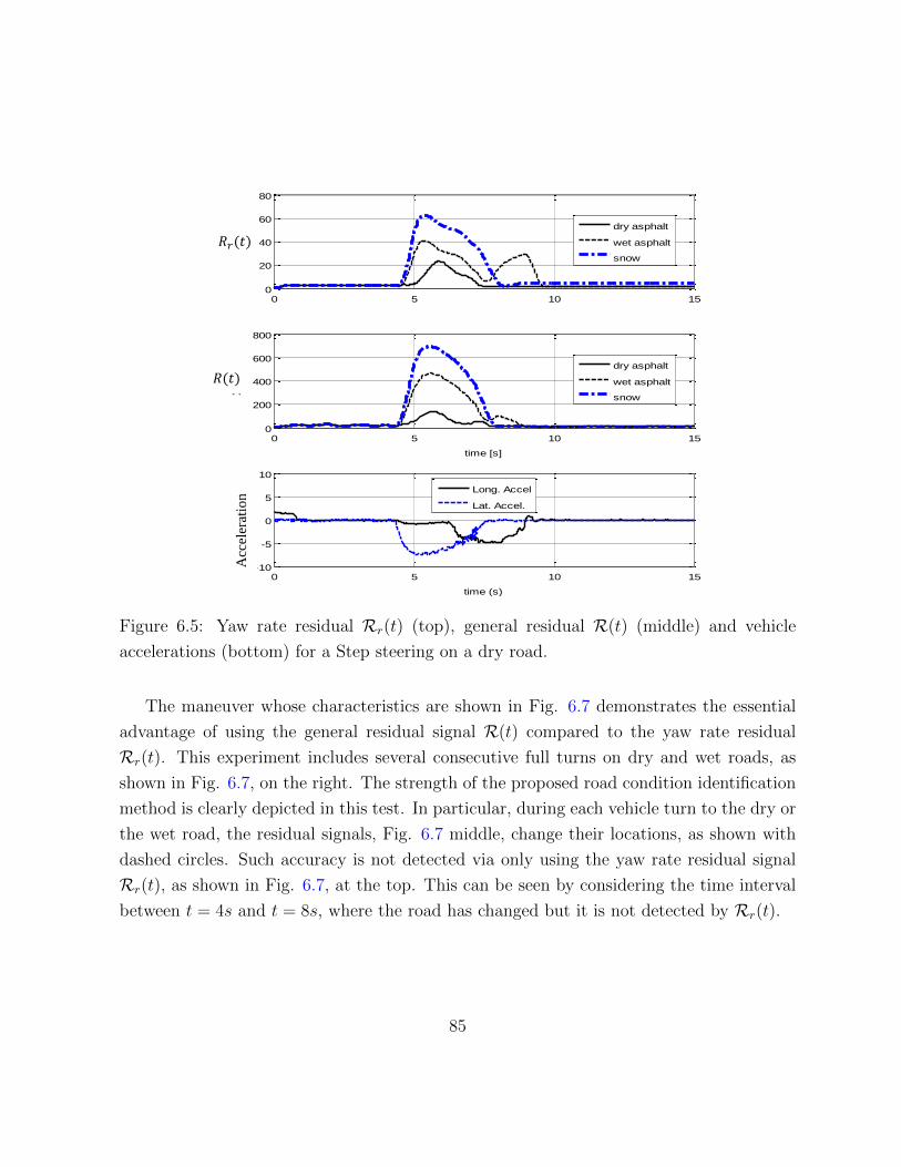
0 5 10 150

20

40

60

80

|e

r|

dry asphalt

wet asphalt

snow

0 5 10 150

200

400

600

800

|e

a|

time [s]

dry asphalt

wet asphalt

snow

0 5 10 15-10

-5

0

5

10

Acc

eler

attio

n (m

/s2)

time (s)

Long. Accel

Lat. Accel.

𝑅𝑟(𝑡)

𝑅(𝑡)

Acc

eler

atio

n

Figure 6.5: Yaw rate residual Rr(t) (top), general residual R(t) (middle) and vehicle

accelerations (bottom) for a Step steering on a dry road.

The maneuver whose characteristics are shown in Fig. 6.7 demonstrates the essential

advantage of using the general residual signal R(t) compared to the yaw rate residual

Rr(t). This experiment includes several consecutive full turns on dry and wet roads, as

shown in Fig. 6.7, on the right. The strength of the proposed road condition identification

method is clearly depicted in this test. In particular, during each vehicle turn to the dry or

the wet road, the residual signals, Fig. 6.7 middle, change their locations, as shown with

dashed circles. Such accuracy is not detected via only using the yaw rate residual signal

Rr(t), as shown in Fig. 6.7, at the top. This can be seen by considering the time interval

between t = 4s and t = 8s, where the road has changed but it is not detected by Rr(t).

85

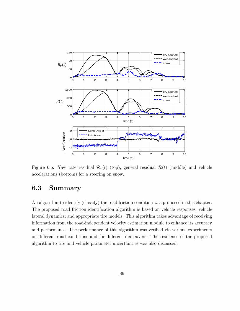
0 1 2 3 4 5 6 7 8 9 100

50

100

150

|e

r|

dry asphalt

wet asphalt

snow

0 1 2 3 4 5 6 7 8 9 100

500

1000

1500

|e

a|

time [s]

dry asphalt

wet asphalt

snow

0 1 2 3 4 5 6 7 8 9 10

-2

0

2

Acc

eler

attio

n (m

/s2)

time (s)

Long. Accel

Lat. Accel.

𝑅𝑟(𝑡)

𝑅(𝑡)

Acc

eler

atio

n

Figure 6.6: Yaw rate residual Rr(t) (top), general residual R(t) (middle) and vehicle

accelerations (bottom) for a steering on snow.

6.3 Summary

An algorithm to identify (classify) the road friction condition was proposed in this chapter.

The proposed road friction identification algorithm is based on vehicle responses, vehicle

lateral dynamics, and appropriate tire models. This algorithm takes advantage of receiving

information from the road-independent velocity estimation module to enhance its accuracy

and performance. The performance of this algorithm was verified via various experiments

on different road conditions and for different maneuvers. The resilience of the proposed

algorithm to tire and vehicle parameter uncertainties was also discussed.

86

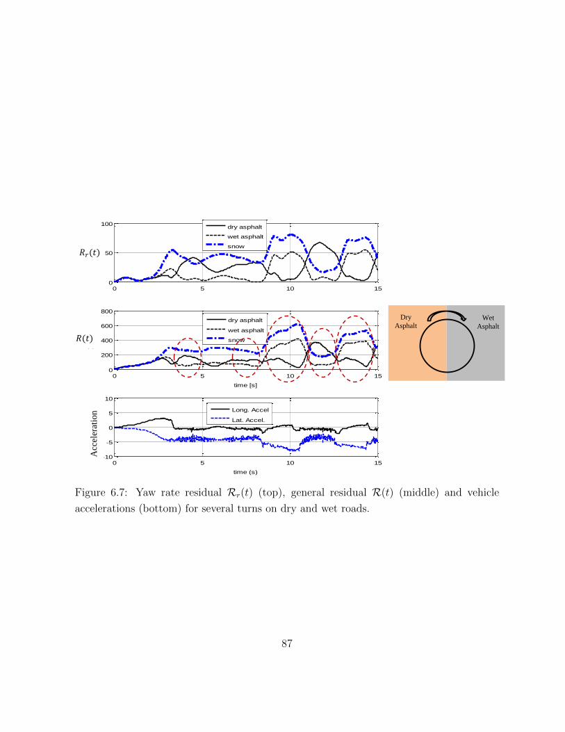
Dry

Asphalt Wet

Asphalt

0 5 10 150

50

100

|e

r|

dry asphalt

wet asphalt

snow

0 5 10 150

200

400

600

800

|e

a|

time [s]

dry asphalt

wet asphalt

snow

0 5 10 15-10

-5

0

5

10

Acc

eler

attio

n (m

/s2)

time (s)

Long. Accel

Lat. Accel.

Acc

eler

atio

n

𝑅(𝑡)

𝑅𝑟(𝑡)

Figure 6.7: Yaw rate residual Rr(t) (top), general residual R(t) (middle) and vehicle

accelerations (bottom) for several turns on dry and wet roads.

87

Chapter 7

Conclusion and Future Works

7.1 Summary and Conclusions

In this thesis, a reliable and resilient corner-based vehicle velocity estimation algorithm

was proposed. This estimator was in the form of a combination of vehicle kinematics and

LuGre tire model. The passivity of the LuGre tire model could help the velocity estimator

improve its performance compared to the previous kinematic based methods. The designed

vehicle velocity estimation algorithm is proven to be resilient to the time-varying tire

parameters, the road friction condition, as well as sensor measurements uncertainties. The

observability of the dynamics as a linear time-varying system, due to the time-varying

wheel speed, was analytically studied prior to designing the observer. One of the featured

advantages of the proposed velocity estimator is that it does not require knowledge about

the road friction condition. Considering the fact that identifying the road condition is hard

in most of the cases, as discussed in Chapter 6, finding a velocity estimation algorithm that

operates independent of the road condition is invaluable. In order to further increase the

performance of the designed velocity estimation algorithm, the effect of the suspension

compliance and the resulting extra degree of freedom was directly added to the estimated

vehicle corner velocity. The performance of the proposed velocity estimation algorithm was

verified via several experimental tests, which were comprised of various standard vehicle

maneuvers performed on different road conditions, and the results showed appropriate

88

correspondence with measurements.

The stability, performance, and robustness of the proposed corner-based vehicle veloc-

ity estimator, from a system theoretic viewpoint, were investigated in this thesis. More

particularly, stability of the observer error dynamics, as a linear-time-varying system, was

proven based on Lyapunov analysis, and a bound on the estimation error, as a function of

road condition and measurements uncertainties, was derived. Other than this analytical

bound, some numerical upper bounds on the estimation error dynamics were presented,

which were based on an input-output approach to the observer error dynamics and their

H∞ performance, and it was shown that the observer error dynamics is a non-expansive

system (i.e., it does not propagate the disturbances to the estimation error). Since real-

time observer gain switching is inevitable in experiments, to change the reliance of the

estimator to measurements in different instances, the stability of the velocity estimator in

the presence of estimation gain switchings was also studied for two cases of arbitrary and

stochastic gain switching scenarios. At the end, the sensitivity of the performance of the

designed velocity estimator to tire parameter variations was investigated. These analyses

were referred to as the offline reliability assessment of the velocity observer in this thesis.

Other than the off-line methods which were investigated as fundamental characteristics

of the designed observer, a real-time reliability measure for the observer was also intro-

duced. The proposed on-line reliability measure is considered to be a milestone that the

observer should reach before its output (estimated states) is used in the control module.

It was based on vehicle kinematics that translate the estimated states (longitudinal and

lateral velocities at each corner) to longitudinal and lateral accelerations, which can be

directly measured in conventional vehicles. After some error clustering, a reliability index

was introduced which showed a level of confidence that one can assign to the estimated

velocities. The proposed on-line reliability measure is tested via several experiments com-

prised of different maneuvers on various road conditions which proved the ability of the

reliability index to diagnose failures in the estimated velocities.

The other main contribution of this thesis was to introduce a road condition identifi-

cation technique. The significance of the proposed method was its simplicity in terms of

implementation as well as its preliminary requirements, compared to the existing meth-

ods in the literature. The proposed road friction identification algorithm was based on

89

vehicle responses to lateral excitations via application of vehicle lateral dynamics and an

appropriate tire model. Both linear and nonlinear (LuGre) tire models were applied to

the vehicle’s lateral dynamics and used in the road condition identification algorithm. One

of the unique features of the proposed road condition identification algorithm is that it

can take advantage of receiving information from the road-independent velocity estimation

module and torque-independent speed estimator [90] to enhance its accuracy and perfor-

mance. The performance of this algorithm was verified via various experiments on different

road conditions and for different maneuvers. The resilience of the proposed algorithm to

tire and vehicle parameter uncertainties was also discussed.

7.2 Future Work

This section provides suggestions on the direction of research required to continue the work

done in this thesis. These avenues of research are presented in two parts: (i) improving

single vehicle estimation, and (ii) taking advantage of networks of vehicles to improve the

estimation. In other words, in this section, some new vistas that should be seriously con-

sidered in estimation and control of future generation of intelligent transportation systems

are introduced. The following subsection pertains to possible future directions in a single

vehicle state estimation as an extension of the work done in this thesis.

7.2.1 Improving Estimation for a Single Vehicle

As a continuation of the work done in this thesis, the following directions are introduced:

1. Improving Corner-Based Velocity Estimation: There are some avenues for en-

hancing the performacne of the proposed corner-based vehicle velocity estimation.

One such direction is to use the known road condition inside the velocity estima-

tion algorithm. As discussed in Chapter 3, the velocity estimation algorithm works

properly despite the fact that the road friction condition is unknown. However, more

knowledge about the road condition results in a less demanding velocity estiamtor

in terms of robustness, which improves the performance of the estimator. To this

90

end, one can use the road condition identification algorithm, presented in Chapter

6 in order to enhance the performance of the velocity estimation. This is shown

schematically with a left-to-right arrow in Fig. 7.1.

Road Cond. Iden. Vehicle Vel. Est

𝜌𝑧 =𝜎0𝑉𝑟

𝜃𝑔(𝑉𝑟) in Equation 3.3 is known

𝑉 𝑥 𝑡 in real time

𝑉 𝑦(0) for refreshing the initial condition

𝑥 = 𝐴𝑥 + 𝐵𝑢 + 𝜌(𝜃)

Equations 3.5 and 3.12

𝑥 = 𝐴(𝑉 𝑥)𝑥 + 𝐵𝛿

𝑥 0 = 𝑓(𝑉 𝑦)

Equations 6.1

Figure 7.1: Reciprocity between vehicle velocity estimation and road condition identifica-

tion.

2. Using Temporal Redundancy for Offline Reliability Measure: As discussed

in Chapter 1, there are two different sets of redundancies which are considered and

used to assess the reliability of systems. One was physical redundancy, which is

based on using multiple sets of infrastructures. The other one is to look at the

history of the system and use its operation throughout the time as a particular

form of redundancy. One can use such an approach in analyzing the performance

of the velocity estimator over time and design a reliability index based on what is

witnessed during the operation of the estimator in a particular time interval. It is

also possible to use the stochastic approach (Markov jump), presented in Chapter 4,

as a probability distribution of fault occurrence to come up with a Bayesian approach

to the behaviour of the estimator throughout the time.

3. Enhancing the Performance of On-line Reliability Measure: The current

reliability index has proven to work properly in different situations; however, there

are some issues needed to be addressed in order to improve its performance. The

main issue is that the reliability index is less sensitive to signal error bias compared

to noises. It is due to the fact that the derivative terms in (5.1) play major roles in

91

detecting faults. Hence, it is imperative to modify the designed reliability measure

to be able to detect small signal error biases.

4. Improving Road Condition Identification Algorithm: There exists a reci-

procity between the vehicle velocity estimation and the road condition identification

algorithms. Such reciprocity is schematically depicted in Fig. 7.1. According to

this figure, specifically, the right-to-left arrow, one can use the velocity estimation

module, which operates independent of the road condition, in order to enhance the

performance of the road condition identification algorithm. More specifically, as the

estimated longitudinal velocity is fed directly to the road condition identification

algorithm and the estimated lateral velocity should also be used after some time

interval to refresh the initial condition of the algorithm, more precise values of the

longitudinal and lateral velocities can definitely improve the performance of the road

condition identification module.

7.2.2 Application of Vehicle Networks to Vehicle State Estima-

tion

The emergence of new generation of communication technologies have brought new avenues

to traditional studies in vehicle estimation and control. The concept of Internet of vehicles,

as a tangible representation of Internet of things, has significantly changed the shape of

the urban transportation. In this direction, one can use the inherent potential in the inter-

vehicle communication to enhance the quality of each individual vehicle estimation and

control strategies. One way is to use information of other vehicles, e.g., their positions,

velocities and accelerations together with algorithms to relate these quantities to the states

of each individual vehicle and find (possible) failures that occur in the velocity estimation

of the vehicle. One such algorithm is schematically shown in Fig. 7.2. As shown in this

figure, vehicle vi gathers information from vehicle vj (in a distributed manner) and then

uses this information to calculate an error function eji ,

eji = κ1

(uij −

∫aijdt

)+ κ2

(uij −

d(pij)

dt

)(7.1)

92

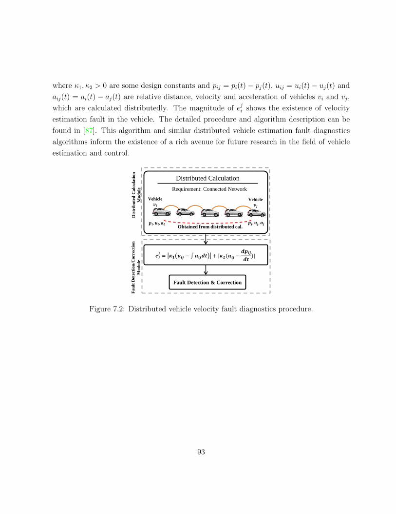
where κ1, κ2 > 0 are some design constants and pij = pi(t)− pj(t), uij = ui(t)− uj(t) and

aij(t) = ai(t) − aj(t) are relative distance, velocity and acceleration of vehicles vi and vj,

which are calculated distributedly. The magnitude of eji shows the existence of velocity

estimation fault in the vehicle. The detailed procedure and algorithm description can be

found in [87]. This algorithm and similar distributed vehicle estimation fault diagnostics

algorithms inform the existence of a rich avenue for future research in the field of vehicle

estimation and control.

Vehicle

𝒗𝒋

Obtained from distributed cal.

Vehicle

𝒗𝒊

𝒑𝒊, 𝒖𝒊, 𝒂𝒊 𝒑𝒋, 𝒖𝒋, 𝒂𝒋

Distributed Calculation

Requirement: Connected Network

Dis

trib

ute

d C

alc

ula

tio

n

Mo

du

le

Fa

ult

Det

ecti

on

/Co

rrec

tio

n

Mo

du

le

𝒆𝒊𝒋= 𝜿𝟏 𝒖𝒊𝒋 − ∫ 𝒂𝒊𝒋𝒅𝒕 + |𝜿𝟐(𝒖𝒊𝒋 −

𝒅𝒑𝒊𝒋

𝒅𝒕)|

Fault Detection & Correction

Figure 7.2: Distributed vehicle velocity fault diagnostics procedure.

93

References

[1] D. Schramm, M. Hiller, and R. Bardini, “Modellbildung und simulation der dynamik

von kraftfahrzeugen,” Springer, 2010.

[2] N. Patel, C. Edwards, and S. Spurgeon, “Tyre-road friction estimationa comparative

study,” Proceedings of the Institution of Mechanical Engineers, Part D: Journal of

Automobile Engineering, vol. 222, no. 12, pp. 2337–2351, 2008.

[3] G. Baffet, A. Charara, and D. Lechner, “Estimation of vehicle sideslip, tire force

and wheel cornering stiffness,” Control Engineering Practice, vol. 17, no. 11, pp.

1255–1264, 2009.

[4] R. Rajamani, G. Phanomchoeng, D. Piyabongkarn, and J. Lew, “Algorithms

for Real-Time Estimation of Individual Wheel Tire-Road Friction Coefficients,”

IEEE/ASME Transactions on Mechatronics, vol. 17, no. 6, pp. 1183–1195, 2012.

[5] M. Doumiati, A. Victorino, D. Lechner, G. Baffet, and A. Charara, “Observers for

vehicle tyre/road forces estimation: experimental validation,” Vehicle System Dy-

namics, vol. 48, no. 11, pp. 1345–1378, 2010.

[6] W. Cho, J. Yoon, S. Yim, B. Koo, and K. Yi, “Estimation of tire forces for application

to vehicle stability control,” IEEE Transactions on Vehicular Technology, vol. 59,

no. 2, pp. 638–649, 2010.

[7] E. Hashemi, A. Kasaeizadeh, A. Khajepour, N. Mushchuk, and S.-K. Chen, “Ro-

bust Estimation and Experimental Evaluation of Longitudinal Friction Forces in

94

Ground Vehicles,” in ASME International Mechanical Engineering Congress Expo-

sition, 2014.

[8] S. Mammar, S. Glaser, and M. Netto, “Vehicle lateral dynamics estimation using

unknown input proportional-integral observers,” in In Proc. American Control Con-

ference, 2006, pp. 1260–1266.

[9] Y. Wang, D. M. Bevly, and S. K. Chen, “Longitudinal Tire Force Estimation with

Unknown Input Observer,” in In Proc. ASME Dynamic Systems and Control Con-

ference, 2012.

[10] Y. Wang, D. M. Bevly, and S.-k. Chen, “Lateral tire force estimation with unknown

input observer,” in In Proc. ASME 5th Annual Dynamic Systems and Control Con-

ference. American Society of Mechanical Engineers, 2012, pp. 531–538.

[11] Y. H. J. Hsu, “Estimation and control of lateral tire forces using steering torque,”

Ph.D. dissertation, Stanford University, 2009.

[12] J. Ryu, “State and parameter estimation for vehicle dynamics control using GPS,”

Ph.D. dissertation, Stanford University, 2004.

[13] J. Ryu and J. C. Gerdes, “Integrating inertial sensors with global positioning system

(GPS) for vehicle dynamics control,” ASME Journal of Dynamic Systems, Measure-

ment, and Control, vol. 126, no. 2, pp. 243–254, 2004.

[14] L. Imsland, T. A. Johansen, T. I. Fossen, H. F. Grip, J. C. Kalkkuhl, and A. Suissa,

“Vehicle velocity estimation using nonlinear observers,” Automatica, vol. 42, no. 12,

pp. 2091–2103, 2006.

[15] J. A. Farrell, H.-S. Tan, and Y. Yang, “Carrier phase GPS-aided INS-based vehicle

lateral control,” ASME Journal of Dynamic Systems, Measurement, and Control,

vol. 125, no. 3, pp. 339–353, 2003.

[16] D. M. Bevly, “Global positioning system (GPS): A low-cost velocity sensor for cor-

recting inertial sensor errors on ground vehicles,” ASME Journal of Dynamic Sys-

tems, Measurement, and Control, vol. 126, no. 2, pp. 255–264, 2004.

95

[17] D. M. Bevly, J. Ryu, and J. C. Gerde, “Integrating INS sensors with GPS measure-

ments for continuous estimation of vehicle sideslip, roll, and tire cornering stiffness,”

IEEE Transactions on Intelligent Transportation Systems, vol. 7, no. 4, pp. 483–493,

2006.

[18] J.-H. Yoon and H. Peng, “A cost-effective sideslip estimation method using velocity

measurements from two GPS receivers,” IEEE Transactions on Vehicular Technology,

vol. 63, no. 6, pp. 2589–2599, 2014.

[19] A. Nishio, K. Tozu, H. Yamaguchi, and K. Asano, “Development of vehicle stability

control system based on vehicle sideslip angle estimation,” SAE Technical Paper,

2001.

[20] Y. Fukada, “Slip-angle estimation for vehicle stability control,” Vehicle System Dy-

namics, pp. 375–388, 1999.

[21] Y.-H. J. Hsu, S. M. Laws, and J. C. Gerdes, “Estimation of tire slip angle and friction

limits using steering torque,” IEEE Transactions on Control Systems Technology,

vol. 18, no. 4, pp. 896–907, 2010.

[22] K. Nam, H. Fujimoto, and Y. Hori, “Lateral stability control of in-wheel-motor-driven

electric vehicles based on sideslip angle estimation using lateral tire force sensors,”

IEEE Transactions on Vehicular Technology, vol. 61, no. 5, pp. 1972–1985, 2012.

[23] C. Ahn, H. Peng, and H. E. Tseng, “Estimation of road friction for enhanced active

safety systems: algebraic approach,” in Proc. Amer. Control Conf, pp. 1104–1109,

2009.

[24] J. Chihoon, S. Hwang, and H. Kim, “Clamping-force control for electromechanical

brake,” IEEE Transactions on Vehicular Technology, vol. 59, no. 7, pp. 3205–3212,

2010.

[25] J. Wang and R. G. Longoria, “Coordinated and reconfigurable vehicle dynamics

control,” IEEE Transactions on Control Systems Technology, 2009.

96

[26] C. Lee, K. Hedrick, and K. S. Yi, “Real-time slip estimation and maximum tireroad

friction coefficient,” IEEE Transactions on Vehicular Technology, vol. 9, pp. 454–458,

2004.

[27] J. O. Hahn, R. Rajamani, and L. Alexander, “GPS-based real-time identification

of tireroad friction coefficient,” IEEE Trans. Control Syst. Technology, vol. 10, pp.

331–343, 2002.

[28] Y. Chen and J. Wang, “Adaptive vehicle speed control with input injections for

longitudinal motion independent road frictional condition estimation,” IEEE Trans-

actions on Vehicular Technology, vol. 60, pp. 839–848, 2011.

[29] H. F. Grip, L. Imsland, T. A. Johansen, T. I. Fossen, J. C. Kalkkuhl, and A. Suissa,

“Nonlinear vehicle side-slip estimation with friction adaptation,” Automatica, vol. 44,

no. 3, pp. 611–622, 2008.

[30] H. Faer Grip, L. Imsland, T. A. Johansen, J. C. Kalkkuhl, and A. Suissa, “Vehicle

sideslip estimation: Design, implementation, and experimental validation,” IEEE

Control Systems, vol. 29, no. 5, pp. 36–52, 2009.

[31] S.-H. You, J.-O. Hahn, and H. Lee, “New adaptive approaches to real-time estimation

of vehicle sideslip angle,” Control Engineering Practice, vol. 17, no. 12, pp. 1367–

1379, 2009.

[32] G. Magallan, C. H. D. Angelo, and G. O. Garcıa, “Maximization of the traction forces

in a 2WD electric vehicle,” IEEE Transactions on Vehicular Technology, vol. 60,

no. 2, pp. 369–380, 2011.

[33] C. C. Wit and P. Tsiotras, “Dynamic Tire Friction Models for Vehicle Traction

Control,” in In Proc. 38th Conference on Decision & Control, 1999, pp. 3746–3751.

[34] X. Zhang, Y. Xu, M. Pan, and F. Ren, “A vehicle ABS adaptive sliding-mode control

algorithm based on the vehicle velocity estimation and tyre/road friction coefficient

estimations,” Vehicle System Dynamics, vol. 52, no. 4, pp. 475–503, 2014.

97

[35] F. Sun, X. Huang, J. Rudolph, and K. Lolenko, “Vehicle state estimation for anti-lock

control with nonlinear observer,” Control Engineering Practice, vol. 43, pp. 69–84,

2015.

[36] S. Antonov, A. Fehn, and A. Kugi, “Unscented kalman filter for vehicle state esti-

mation,” Vehicle System Dynamics, vol. 49, no. 9, pp. 1497–1520, 2011.

[37] M. Gadola, D. Chindamo, M. Romano, and F. Padula, “Development and validation

of a kalman filter-based model for vehicle slip angle estimation,” Vehicle System

Dynamics, vol. 52, no. 1, pp. 68–84, 2014.

[38] H. B. Pacejka and R. S. Sharp, “Shear Force Development by Pneumatic Tyres in

Steady State Conditions: A Review of Modelling Aspects,” Vehicle System Dynam-

ics, vol. 20, no. 3-4, pp. 121–175, 1991.

[39] R. T. Uil, “Tyre Models for Steady-State Vehicle Handling Analysis,” Ph.D. disser-

tation, Eindhoven University of Technology, 2007.

[40] J. Deur, J. Asgari, and D. Hrovat, “A 3D Brush-Type Dynamic Tire Friction Model,”

Vehicle System Dynamics, vol. 42, no. 3, pp. 133–173, 2004.

[41] W. Liang, J. Medanic, and R. Ruhl, “Analytical Dynamic Tire Model,” Vehicle

System Dynamics, vol. 46, pp. 197–227, 2008.

[42] C. C. Wit and R. Horowitz, “Observer for Tire/Road Contact Friction Using Only

Wheel Angular Velocity Information,” in In Proc. 38th Conference on Decision &

Control, 1999, pp. 3932–3937.

[43] C. Wit, P. Tsiotras, E. Velenis, M. Gissinger, and G. Gissinger, “Dynamic Friction

Models for Road/Tire Longitudinal Interaction,” Vehicle System Dynamics, vol. 39,

pp. 189–226, 2003.

[44] P. Tsiotras, E. Velenis, and M. Sorine, “A LuGre Tire Friction Model With Exact

Aggregate Dynamics,” Vehicle System Dynamics, vol. 42, pp. 195–210, 2004.

98

[45] C. C. Wit, H. Olsson, K. J. Astrom, and P. Lischinsky, “A New Model for Control

of Systems with Friction,” IEEE Transactions on Automatic Control, vol. 40, 1995.

[46] K. J. Astrom and C. C. Wit, “Revisiting the LuGre Model,” IEEE Control System

Magazine, vol. 6, pp. 101–114, 2008.

[47] E. Hashemi, M. Pirani, A. Khajepour, and A. Kasaiezadeh, “A comprehensive study

on the stability analysis of vehicle dynamics with pure/combined-slip tyre models,”

Vehicle System Dynamics, vol. 54, no. 12, pp. 1736–1761, 2016.

[48] C. Ahn, H. Peng, and H. Tseng, “Robust Estimation of Road Friction Coefficient,”

in In Proc. American Control Conference, no. 3, 2011, pp. 3948–3953.

[49] W. Cho, J. Yoon, S. Yim, B. Koo, and K. Yi, “Estimation of tire forces for application

to vehicle stability control,” IEEE Transactions on Vehicular Technology, vol. 59,

no. 2, pp. 638–649, 2010.

[50] E. Hashemi, M. Pirani, A. Khajepour, B. Fidan, A. Kasaiezadeh, S. Chen, and

B. Litkouhi, “Integrated estimation structure for the tire friction forces in ground

vehicles,” in In Proc. IEEE Conference on Advanced Intelligent Mechatronics. IEEE,

2016.

[51] H. J. LeBlanc, H. Zhang, X. Koutsoukos, and S. Sundaram, “Resilient asymptotic

consensus in robust networks,” IEEE Journal on Selected Areas in Communications,

vol. 31, pp. 766–781, 2013.

[52] K. Stouffer, J. Falco, and K. Scarfone., “Guide to industrial control systems security,”

National Institute of Standards and Technology, 2008.

[53] A. Cardenas, S. Amin, , and S. S. Sastry, “Research challenges for security of control

systems,” 3rd USENIX Workshop on Hot Topics in Security, 2008.

[54] R. Isermann, “Supervision, fault-detection and fault-diagnosis methods an introduc-

tion,” Control Engineering Practice, vol. 5, pp. 639–652, 1997.

99

[55] J. von Neumann, “Probabilistic logics and the synthesis of reliable organisms from

unreliable components,” Princeton University Press, 1956.

[56] E. Y. Chow and A. S. Willsky, “Analytical redundancy and the design of robust

failure detection systems,” IEEE Transactions on Automatic Control, pp. 603–614,

1984.

[57] M. Blanke, M. Kinnaert, J. Lunze, and M. Staroswiecki, “Diagnosis and fault- toler-

ant control,” Springer, 2006.

[58] R. Isermann, “Model-based fault detection and diagnosis: status and applications,”

16th IFAC Symposium on Automatic Control in Aerospace, pp. 71–85, 2004.

[59] H. K. Khalil and J. W. Grizzle, “Nonlinear systems,” Prentice hall, 1996.

[60] K. Zhou, J. C. Doyle, and K. Glover, “Robust and optimal control,” Prentice Hall,

1996.

[61] D. Liberzon, “Switching in systems and control,” Springer, 2012.

[62] H. Lin and P. J. Antsaklis, “Stability and stabilizability of switched linear systems:

a survey of recent results,” IEEE Transactions on Automatic Control, pp. 308–322,

2009.

[63] O. L. V. Costa, M. D. Fragoso, and R. P. Marques, “Discrete time markovian jump

linear systems,” Springer-Verlag, 2005.

[64] ——, “Continuous time markovian jump linear systems,” Springer-Verlag, 2005.

[65] M. Karan, P. Shi, and C. Y. Kaya, “Transition probability bounds for the stochastic

stability robustness of continuous- and discrete-time markovian jump linear systems,”

Automatica, p. 21592168, 2006.

[66] J. L. Xiong, J. Lam, H. J. Gao, and W. C. Daniel, “On robust stabilization of

markovian jump systems with uncertain switching probabilities,” Automatica, vol. 41,

pp. 897–903, 2005.

100

[67] R. Krtolica, U. Ozguner, H. Chan, H. Goktas, J. Winkelman, and M. Liubakka,

“Stability of linear feedback systems with random communication delays,” Int. J.

Control, vol. 54, pp. 925–953, 1994.

[68] P. Seiler and R. Sengupta, “Analysis of communication losses in vehicle control prob-

lems,” In Proc. American Control Conference, pp. 1491–1496, 2001.

[69] L. Zhang and E. Boukas, “Stability and stabilization of markovian jump linear sys-

tems with partly unknown transition probabilities,” Automatica, vol. 45, pp. 463–468,

2009.

[70] M. Pirani, E. Hashemi, A. Khajepour, B. Fidan, A. Kasaiezadeh, S. Chen, and

B. Litkouhi, “Resilient corner based vehicle velocity estimation,” IEEE Transactions

on Control Systems Technology, 2017.

[71] E. Hashemi, M. Pirani, A. Khajepour, A. Kasaiezadeh, S.-K. Chen, and B. Litk-

ouhi, “Corner-based estimation of tire forces and vehicle velocities robust to road

conditions,” Control Engineering Practice, vol. 61, pp. 28–40, 2017.

[72] E. Hashemi, “Full Vehicle State Estimation Using a Holistic Corner-based Ap-

proach,” Ph.D. dissertation, University of Waterloo, 2017.

[73] E. Hashemi, S. Khosravani, A. Khajepour, A. Kasaiezadeh, S.-K. Chen, and B. Litk-

ouhi, “Longitudinal vehicle state estimation using nonlinear and parameter-varying

observers,” Mechatronics, vol. 43, pp. 28–39, 2017.

[74] R. Toth, Modeling and Identification of Linear Parameter-Varying Systems.

Springer, 2010.

[75] E. Hashemi, R. Zarringhalam, A. Khajepour, W. Melek, A. Kasaiezadeh, and S.-K.

Chen, “Real-time estimation of the road bank and grade angles with unknown input

observers,” Vehicle System Dynamics, vol. 55, no. 5, pp. 648–667, 2017.

[76] J. E. Slotine and W. Li, “Applied nonlinear control,” Prentice Hall, 1991.

101

[77] A. Czornik, A. Nawrat, M. Niezabitowski, and A. Szyda, “On the lyapunov and

bohl exponent of time-varying discrete linear system,” In Proc. 20th Mediterranean

Conference on Control and Automation (MED), pp. 194–197, 2012.

[78] T. Berger, “Bohl exponent for time-varying linear differential-algebraic equations,”

Int. J. Control, vol. 85, pp. 1433–1451, 2012.

[79] H. Lin and P. J. Antsaklis, “Stability and stabilizability of switched linear systems:

a survey of recent results,” IEEE Transactions on Automatic control, vol. 54, no. 2,

pp. 308–322, 2009.

[80] D. Liberzon, Switching in systems and control. Boston, MA, USA: Birkhuser, 2003.

[81] T. B. Hoang, W. P. Lepine, A. D. Bernardinis, and M. Netto, “Extended braking

stiffness estimation based on a switched observer, with an application to wheel-

acceleration control,” IEEE Transactions on Control Systems Technology, vol. 22,

no. 6, pp. 2384 – 2392, 2014.

[82] V. Gupta, R. M. Murray, and B. Hassibi, “On the control of jump linear markov

systems with markov state estimation,” In Proc. American Control Conference, pp.

2893 – 2898, 2003.

[83] V. Dragan and T. Morozan, “Observability and detectability of a class of discrete-

time stochastic linear systems,” IMA Journal of Mathematical Control and Informa-

tion, vol. 23, pp. 371–394, 2006.

[84] R. Zarringhalam, A. Rezaeian, A. Khajepour, and W. Melek, “Vehicle sensor failure

detection and fault-tolerant estimation of states,” Symposium on Advanced Intelligent

Systems, 2012.

[85] M. Pirani and S. Sundaram, “On the smallest eigenvalue of grounded Laplacian

matrices,” IEEE Transactions on Automatic Control, vol. 61, no. 2, pp. 509–514,

2016.

[86] M. Pirani, E. M. Shahrivar, B. Fidan, and S. Sundaram, “Robustness of leader -

follower networked dynamical systems,” arXiv:1604.08651v1, 2016.

102

[87] M. Pirani, E. Hashemi, A. Khajepour, B. Fidan, B. Litkouhi, and S. K. Chen, “Co-

operative vehicle speed fault diagnostics and correction,” arXiv:1706.09447, 2017.

[88] E. Hashemi, M. Pirani, B. Fidan, A. Khajepour, and S. C. A. Kasaiezadeh, “Dis-

tributed robust vehicle state estimation,” IEEE Intelligent Vehicles Symposium, pp.

693–698, 2017.

[89] E. Hashemi, M. Pirani, A. Khajepour, B. Fidan, and S. C. A. Kasaiezadeh, “Opinion

dynamics based vehicle velocity estimation and diagnosis,” IEEE Transaction on

Intelligent Transportation Systems, submitted, 2017.

[90] A. Kasaiezadeh, E. Hashemi, A. Khajepour, B. Litkouhi, and S.-K. Chen, “Corner-

based longitudinal speed estimation,” 2016, uS Pending Patent.

[91] N. Kazantzis and C. Kravaris, “Time-discretization of nonlinear control systems via

taylor methods,” Computers and Chemical Engineering, vol. 23, pp. 763–784, 1999.

[92] U. Kiencke, “Real-Time Estimation of Adhesion Characteristic Between Tires and

Road,” in In Proc. of IFAC World Congress, 1993.

[93] U. W. Kiencke and A. Daiss, “Estimation of Tyre Friction for Enhanced ABS-

Systems,” in In Proc. of International Symposium on Advanced Vehicle Control,

1994.

[94] Y. H. Judy and J. C. Gerdes, “The predictive nature of pneumatic trail: Tire slip

angle and peak force estimation using steering torque,” in AVEC08, 2008.

[95] F. Garofalo, G. Celentano, and L. Glielmo, “Stability Robustness of Interval Matrices

Via Lyapunov Quadratic Forms,” IEEE Transactions on Automatic Control, vol. 38,

no. 2, pp. 281–284, 1993.

[96] P. Gahinet, P. Apkarian, and M. Chilali, “Affine Parameter-Dependent Lyapunov

Functions and Real Parametric Uncertainty,” IEEE Transactions on Automatic Con-

trol, vol. 41, no. 3, pp. 436–442, 1996.

103

[97] C. Ahn, H. Peng, and H. E. Tseng, “Estimation of road friction for enhanced active

safety systems: Dynamic approach,” in Proc. Amer. Control Conf, pp. 1110–1115,

2009.

[98] P. A. Bliman, T. Bonald, and M. Sorine, “Hysteresis operators and tire friction mod-

els: Application to vehicle dynamic simulations,” Proc. of the International Council

for Industrial and Applied Mathematics, 1995.

[99] A. V. Zanten, R. Erhardt, and G. Pfaff, “The vehicle dynamics control system of

bosch,” SAE Technical Paper-950759, 1995.

[100] A. V. Zanten, “Evolution of electronic control systems for improving the vehicle

dynamic behavior,” International Symposium on Advanced Vehicle Control,, 2002.

[101] D. Gebre-Egziabher, R. C. Hayward, and J. D. Powell, “A low-cost GPS/inertial at-

titude heading reference system (AHRS) for general aviation applications,” Position

location and navigation symposium, 1998.

[102] A. Hac and M. Simpson, “Estimation of vehicle side slip angle and yaw rate,” SAE

Technical Paper, 2000.

[103] K. Kobayashi, K. Watanabe, and C. Science, “Estimation of absolute vehicle speed

using fuzzy logic rule-based kalman filter,” In Proc. American Control Conference,

1995.

[104] C. Canudas-De-Wit, M. L. Petersen, and A. Shiriaev, “A new nonlinear observer for

tire/road distributed contact friction,” In Proc. 42nd IEEE Conference on Decision

and Control, 2003.

[105] M. Hiemer, A. V. Vietinghoff, U. Kiencke, and T. Matsunaga, “Determination of

the vehicle body side slip angle with non-linear observer strategies,” SAE Technical

Paper, 2005.

[106] L. Imsland, T. A. Johansen, T. I. Fossen, J. C. Kalkkuhl, and A. Suissa, “Vehicle

velocity estimation using modular nonlinear observers,” Proc. 44th IEEE Conference

on Decision and Control, 2005.

104

[107] R. Wang and J. Wang, “Tire–road friction coefficient and tire cornering stiffness es-

timation based on longitudinal tire force difference generation,” Control Engineering

Practice, vol. 21, no. 1, pp. 65–75, 2013.

[108] Y. Chen and J. Wang, “Adaptive vehicle speed control with input injections for

longitudinal motion independent road frictional condition estimation,” IEEE Trans-

actions on Vehicular Technology, vol. 60, no. 3, pp. 839–848, 2011.

[109] M. Choi, J. J. Oh, and S. B. Choi, “Linearized recursive least squares methods

for real-time identification of tire–road friction coefficient,” IEEE Transactions on

Vehicular Technology, vol. 62, no. 7, pp. 2906–2918, 2013.

[110] J. Rath, K. Veluvolu, and M. Defoort, “Simultaneous estimation of road profile and

tyre road friction for automotive vehicle,” IEEE Transactions on Vehicular Technol-

ogy, vol. 64, no. 10, pp. 4461–4471, 2014.

[111] M. Doumiati, A. Victorino, A. Charara, and D. Lechner, “Lateral load transfer

and normal forces estimation for vehicle safety: experimental test,” Vehicle System

Dynamics, vol. 47, no. 12, pp. 1511–1533, 2009.

[112] K. Nam, S. Oh, H. Fujimoto, and Y. Hori, “Estimation of sideslip and roll angles

of electric vehicles using lateral tire force sensors through rls and kalman filter ap-

proaches,” IEEE Transactions on Industrial Electronics, vol. 60, no. 3, pp. 988–1000,

2013.

[113] E. Kayacan, E. Kayacan, H. Ramon, and W. Saeys, “Distributed nonlinear model

predictive control of an autonomous tractor–trailer system,” Mechatronics, vol. 24,

no. 8, pp. 926–933, 2014.

[114] B. Li, H. Du, W. Li, and Y. Zhang, “Side-slip angle estimation based lateral dynamics

control for omni-directional vehicles with optimal steering angle and traction/brake

torque distribution,” Mechatronics, 2014.

[115] H. Dugoff, P. Fancher, and L. Segel, “An analysis of tire traction properties and their

influence on vehicle dynamic performance,” SAE Technical Paper, Tech. Rep., 1970.

105

[116] H. Zhang, X. Huang, J. Wang, and H. R. Karimi, “Robust energy-to-peak sideslip

angle estimation with applications to ground vehicles,” Mechatronics, 2014.

[117] F. Sun, K. Lolenko, and J. Rudolph, “Nonlinear observer design for state estimation

during antilock braking,” Proceedings of the Institution of Mechanical Engineers,

Part I: Journal of Systems and Control Engineering, vol. 228, no. 2, pp. 78–86, 2014.

[118] L. Imsland, T. Johansen, T. Fossen, J. Kalkkuhl, and A. Suissa, “Vehicle Velocity

Estimation using Modular Nonlinear Observers,” in In Proc. 44th IEEE Conference

on Decision and Control, 2005, pp. 6728–6733.

106