RELIABILITY/AVAILABILITY OF ELECTRICAL & MECHANICAL ...

TM 5-698-1

TECHNICAL MANUAL

RELIABILITY/AVAILABILITY OF ELECTRICAL & MECHANICAL

SYSTEMS FOR COMMAND, CONTROL, COMMUNICATIONS,

COMPUTER, INTELLIGENCE, SURVEILLANCE AND

RECONNAISSANCE (C4ISR) FACILITIES

APPROVED FOR PUBLIC RELEASE: DISTRIBUTION IS UNLIMITED

HEADQUARTERS, DEPARTMENT OF THE ARMY 19 JANUARY 2007

Downloaded from http://www.everyspec.com

TM 5-698-1

REPRODUCTION AUTHORIZATION/RESTRICTIONS

This manual has been prepared by or for the Government and, except to the ex-tent indicated below, is public property and not subject to copyright. Reprint or republication of this manual should include a credit substantially at follows: "Department of the Army, TM 5-698-1, Reliability/Availability of Electrical & Mechanical Systems for Command, Control, Communications, Computer, Intelligence, Surveillance, and Reconnaissance (C4ISR) Facilities, 19 January 2007.


TM 5-698-1

This manual supersedes TM 5-698-1 dated 14 March 2003 i

Technical Manual HEADQUARTERS No. 5-698-1 DEPARTMENT OF THE ARMY Washington, DC, 19 January 2007

APPROVED FOR PUBLIC RELEASE: DISTRIBUTION IS UNLIMITED

RELIABILITY/AVAILABILITY OF ELECTRICAL & MECHANICAL SYSTEMS FOR COMMAND, CONTROL, COMMUNICATIONS,

COMPUTER, INTELLIGENCE, SURVEILLANCE, AND RECONNAISSANCE (C4ISR) FACILITIES

CONTENTS Paragraph Page CHAPTER 1. INTRODUCTION Purpose....................................................................................................... 1-1 1-1 Scope.......................................................................................................... 1-2 1-1 References.................................................................................................. 1-3 1-1 Definitions.................................................................................................. 1-4 1-1 Historical perspective................................................................................. 1-5 1-2 Relationship among reliability, maintainability, and availability .............. 1-6 1-3 The importance of availability and reliability to C4ISR facilities ............. 1-7 1-3 Improving availability of C4ISR facilities................................................. 1-8 1-4 CHAPTER 2. BASIC RELIABILITY AND AVAILABILITY CONCEPTS Probability and statistics ............................................................................ 2-1 2-1 Calculating reliability................................................................................. 2-2 2-4 Calculating availability .............................................................................. 2-3 2-6 Predictions and assessments....................................................................... 2-4 2-9 CHAPTER 3. IMPROVING AVAILABILITY OF C4ISR FACILITIES Overview of the process............................................................................. 3-1 3-1 New facilities ............................................................................................. 3-2 3-1 Existing facilities ....................................................................................... 3-3 3-4 Improving availability through addition of redundancy ............................ 3-4 3-5 Improving availability through reliability-centered maintenance (RCM) . 3-5 3-12 Application of RCM to C4ISR facilities.................................................... 3-6 3-15 CHAPTER 4. ASSESSING RELIABILITY AND AVAILABILITY OF C4ISR FACILITIES Purpose of the assessment.......................................................................... 4-1 4-1 Prediction ................................................................................................... 4-2 4-1 Analytical Methodologies .......................................................................... 4-3 4-2 Analysis Considerations............................................................................. 4-4 4-6 Modeling Examples .................................................................................. 4-5 4-7 Modeling Complexities.............................................................................. 4-6 4-13 Conclusion ................................................................................................. 4-7 4-15


TM 5-698-1

ii

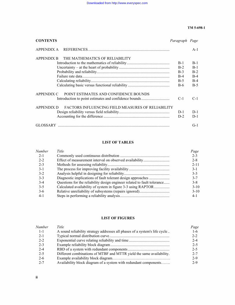
CONTENTS Paragraph Page APPENDIX A REFERENCES.................................................................................... A-1 APPENDIX B THE MATHEMATICS OF RELIABILITY Introduction to the mathematics of reliability ............................................ B-1 B-1 Uncertainty – at the heart of probability .................................................... B-2 B-1 Probability and reliability........................................................................... B-3 B-2 Failure rate data.......................................................................................... B-4 B-4 Calculating reliability................................................................................. B-5 B-4 Calculating basic versus functional reliability ........................................... B-6 B-5 APPENDIX C POINT ESTIMATES AND CONFIDENCE BOUNDS Introduction to point estimates and confidence bounds ............................. C-1 C-1 APPENDIX D FACTORS INFLUENCING FIELD MEASURES OF RELIABILITY Design reliability versus field reliability.................................................... D-1 D-1 Accounting for the difference .................................................................... D-2 D-1 GLOSSARY ................................................................................................................... G-1

LIST OF TABLES

Number Title Page 2-1 Commonly used continuous distribution ................................................... 2-3 2-2 Effect of measurement interval on observed availability........................... 2-8 2-3 Methods for assessing reliability................................................................ 2-11 3-1 The process for improving facility availability .......................................... 3-1 3-2 Analysis helpful in designing for reliability............................................... 3-3 3-3 Diagnostic implications of fault tolerant design approaches ..................... 3-7 3-4 Questions for the reliability design engineer related to fault tolerance...... 3-8 3-5 Calculated availability of system in figure 3-3 using RAPTOR................ 3-10 3-6 Relative unreliability of subsystems (repairs ignored)............................... 3-10 4-1 Steps in performing a reliability analysis................................................... 4-1

LIST OF FIGURES

Number Title Page 1-1 A sound reliability strategy addresses all phases of a system's life cycle .. 1-6 2-1 Typical normal distribution curve.............................................................. 2-2 2-2 Exponential curve relating reliability and time.......................................... 2-4 2-3 Example reliability block diagram............................................................. 2-5 2-4 RBD of a system with redundant components ........................................... 2-5 2-5 Different combinations of MTBF and MTTR yield the same availability. 2-7 2-6 Example availability block diagram……………………………………… 2-9 2-7 Availability block diagram of a system with redundant components……. 2-9


TM 5-698-1

This manual supersedes TM 5-698-1 dated 14 March 2003 iii

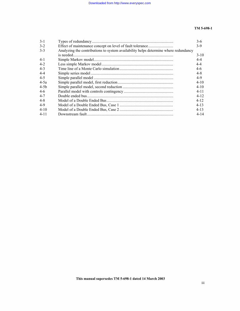
3-1 Types of redundancy.................................................................................. 3-6 3-2 Effect of maintenance concept on level of fault tolerance ......................... 3-9 3-3 Analyzing the contributions to system availability helps determine where redundancy is needed..................................................................................................... 3-10 4-1 Simple Markov model................................................................................ 4-4 4-2 Less simple Markov model ........................................................................ 4-4 4-3 Time line of a Monte Carlo simulation ...................................................... 4-6 4-4 Simple series model ................................................................................... 4-8 4-5 Simple parallel model ................................................................................ 4-9 4-5a Simple parallel model, first reduction........................................................ 4-10 4-5b Simple parallel model, second reduction ................................................... 4-10 4-6 Parallel model with controls contingency .................................................. 4-11 4-7 Double ended bus....................................................................................... 4-12 4-8 Model of a Double Ended Bus................................................................... 4-12 4-9 Model of a Double Ended Bus, Case 1 ...................................................... 4-13 4-10 Model of a Double Ended Bus, Case 2 ...................................................... 4-13 4-11 Downstream fault....................................................................................... 4-14


TM 5-698-1

1-1

CHAPTER 1 INTRODUCTION

1-1 Purpose The purpose of this technical manual is to provide facility managers with the information and procedures necessary to baseline the reliability and availability of their facilities, identify "weak links", and to provide guidance toward cost-effective strategies of improving reliability and availability. 1-2 Scope The information in this manual reflects both the move to incorporate commercial practices and the lessons learned over many years of acquiring weapon systems. It specifically addresses electrical and mechanical systems for command, control, communications, computer, intelligence, surveillance and reconnaissance (C4ISR) facilities, focusing on the role reliability, availability, and maintainability (RAM) criteria play in supporting the mission. The manual, in the spirit of the new policies regarding acquisition and evaluation, describes the objectives of a sound strategy and the tools available to meet these objectives. 1-3. References Appendix A contains a complete listing of references used in this manual. Of particular interest are related reliability disciplines that include Reliability Centered Maintenance for C4ISR Facilities (RCM, Technical Manual (TM 5-698-2), Reliability Primer for C4ISR Facilities (TM 5-698-3), Failure Modes and Effects Analysis for C4ISR Facilities (FMECA, TM 5-698-4), Survey of Reliability and Availability Information for Power Distribution, Power Generation and Heating, Ventilating and Air Conditioning (HVAC) Components for Commercial, Industrial and Utility Installations (TM 5-698-5) and the Reliability Data Collection Manual (TM 5-698-6). 1-4. Definitions The three key terms used in this TM are availability, reliability, and maintainability. Additional terms and abbreviations used in this manual are explained in the glossary. a. Availability. Availability is defined as the percentage of time that a system is available to perform its required function(s). It is measured in a variety of ways, but it is principally a function of downtime. Availability can be used to describe a component or system but it is most useful when describing the nature of a system of components working together. Because it is a fraction of time spent in the “available” state, the value can never exceed the bounds of 0 < A < 1. Thus, availability will most often be written as a decimal, as in 0.99999, as a percentage, as in 99.999%, or equivalently spoken, “five nines of availability.” Chapter 2 contains a detailed discussion of availability.

b. Reliability. Reliability is concerned with the probability and frequency of failures (or more correctly, the lack of failures). A commonly used measure of reliability for repairable systems is the mean time between failures (MTBF). The equivalent measure for non-repairable items is mean time to failure (MTTF). Reliability is more accurately expressed as a probability of success over a given duration of time, cycles, etc. For example, the reliability of a power plant might be stated as 95% probability of no failure over a 1000-hour operating period while generating a certain level of power. (Note that the electrical power industry has historically not used the definitions given here for reliability. The industry


TM 5-698-1

1-2

defines reliability as the percentage of time that a system is available to perform its function; i.e., availability. The relationship between reliability and availability is discussed in paragraph 1-6.) c. Maintainability. Maintainability is defined as the measure of the ability of an item to be restored or retained in a specified condition. Maintenance should be performed by personnel having specified skill levels, using prescribed procedures and resources, at each prescribed level of maintenance and repair. Simply stated, maintainability is a measure of how effectively and economically failures can be prevented through preventive maintenance and how quickly system operation can be restored following a failure through corrective maintenance. A commonly used measure of maintainability in terms of corrective maintenance is the mean time to repair (MTTR). Note that maintainability is not the same as maintenance. Maintainability is a design parameter, while maintenance consists of actions to correct or prevent a failure event. d. Reliability Centered Maintenance. A burgeoning application of the three definitions mentioned above is the Reliability Centered Maintenance (RCM). An RCM program is instrumental for a number of reasons. (1) It helps to maximize effectiveness of the maintenance resources by focusing attention of preventative maintenance (PM) programs toward components with predictable failure distributions (i.e. predictable wear out). (2) It provides the means to gather actual RAM data from the facility itself to augment the generic component data initially implemented. 1-5. Historical perspective In measuring the performance of electrical and mechanical systems for C4ISR facilities, availability is of critical concern. The level of availability achieved in operation is determined by many factors, but arguably the two most important factors are reliability and maintainability. Reliability and maintainability (R&M) are two disciplines that have increased in importance over the past 30 years as systems have become more complex, support costs have increased, and defense budgets have decreased. Both disciplines, however, have been developing for much longer than 30 years. a. Reliability. Reliability, for example, has been a recognized performance factor for at least 50 years. During World War II, the V-1 missile team, led by Dr. Wernher von Braun, developed what was probably the first reliability model. The model was based on a theory advanced by Eric Pieruschka that if the probability of survival of an element is 1/x, then the probability that a set of n identical elements will survive is (1/x)n. The formula derived from this theory is sometimes called Lusser's law (Robert Lusser is considered a pioneer of reliability) but is more frequently known as the formula for the reliability of a series system: Rs = R1 x R2 x . . . x Rn. b. Availability. Practical, data based availability studies have their origins with electrical and mechanical data collected by the Institute of Electrical and Electronics Engineers (IEEE) and the US Army Corps of Engineers. Data gathered by these organizations has made years of developed theory and analysis possible. Use of software in advanced availability calculations has led the way for simulation applications as more complex data is collected. c. Maintainability. Maintainability is perhaps less fully developed as a technical discipline than is reliability. Maintainability is a measure of the relative ease and economy of time and resources with which maintenance can be performed. Maintainability is a function of design features, such as access,


TM 5-698-1

1-3

interchangeability, standardization, and modularity. Maintainability includes designing with the human element of the system in mind. The human element includes operators and maintenance personnel. 1-6. Relationship among reliability, maintainability, and availability Perfect reliability (i.e., no failures, ever, during the life of the system) is difficult to achieve. Even when a "good" level of reliability is achieved, some failures are expected. The effects of failures on the availability and support costs of repairable systems can be minimized with a "good" level of maintainability. A system that is highly maintainable can be restored to full operation in a minimum of time with a minimum expenditure of resources. a. Inherent availability. When only reliability and corrective maintenance or repair (i.e., design) effects are considered, we are dealing with inherent availability. This level of availability is solely a function of the inherent design characteristics of the system. b. Operational availability. Availability is determined not only by reliability and repair, but also by other factors related to preventative maintenance and logistics. When these effects of preventative maintenance and logistics are included, we are dealing with operational availability. Operational availability is a "real-world" measure of availability and accounts for delays such as those incurred when spares or maintenance personnel are not immediately at hand to support maintenance. Availability is discussed in more detail in chapter 2. Inherent and operational reliability are discussed further in appendix D. 1-7. The importance of availability and reliability to C4ISR facilities C4ISR facilities support a variety of missions. Often these missions are critical and any downtime is costly, in terms of economic penalties, loss of mission, or injury or death to personnel. For that reason, importance of availability is paramount to C4ISR facilities. This section gives an introduction to the application of RAM criteria in C4ISR facilities; a more exhaustive explanation begins in chapter 3. a. Availability. Availability of a system in actual field operations is determined by the following. (1) The frequency of occurrence of failures. These failures may prevent the system from performing its function (mission failures) or cause a degraded system effect. This frequency is determined by the system's level of reliability. (2) The time required restoring operations following a system failure or the time required to perform maintenance to prevent a failure. These times are determined in part by the system's level of maintainability. (3) The logistics provided to support maintenance of the system. The number and availability of spares, maintenance personnel, and other logistics resources combined with the system's level of maintainability determine the total downtime following a system failure. b. Reliability. Reliability is a measure of a system's performance that affects availability, mission accomplishment, and operating and support (O&S) costs. Too often we think of performance only in terms of voltage, capacity, power, and other "normal" measures. However, high frequency of system failures can be overshadowing the importance of more typical system metrics.


TM 5-698-1

1-4

c. Reliability, trust, and safety. The importance of reliability is evident everywhere. When we begin a road trip in the family automobile, we do so with the assumption that the car will not break down. We are, perhaps unconsciously, assuming that the car has an inherent level of reliability. Similarly, we have a certain level of trust that airliners, elevators, and appliances will operate with little chance of failure. In dealing with systems where failure can result in injury or death, the distinction between reliability and safety becomes blurred. Reliability affects safety; preventing injury and promoting reliability can often be accomplished in the same stroke. d. Reliability and costs. Reliability also affects the costs to own and operate a system. Again using the example of the family automobile, the cost of ownership includes gas and oil, insurance, repairs, and replacement of tires and other "expendables." Reliability determines how often repairs are needed. The less often the car has a failure, the less it will cost to operate over its life. The reliability of any repairable system is a significant factor in determining the long-term costs to operate and support the system. For non-repairable systems, the cost of failure is the loss of the function (e.g., the missile misses its target, the fuse fails to protect a circuit, etc.). e. The inevitability of failures. Regardless of how reliable a system may be, failures will occur. An effective maintenance program applied to a system that has been designed to be maintainable is necessary to deal with the certainty of failure. Even when several redundant items are installed to decrease the chance of a mission failure, when any one item fails, it must be repaired or replaced to retain the intended level of redundancy. 1-8. Improving availability of C4ISR facilities The decision on which methods to use for improving availability depends on whether the facility is being designed and developed or is already in use. a. Existing C4ISR facilities. For a facility that is being operated, three basic methods are available for improving availability when the current level of availability is unacceptable: selectively adding redundant units (e.g., generators, chillers, fuel supply, etc.) to eliminate sources of single-point failure; optimizing maintenance using a reliability-centered maintenance (RCM) approach to minimize downtime; or redesign subsystems or to replace components and subsystems with higher reliability items. Of course, some combination of these three methods can also be implemented. These methods will be discussed in more detail in chapter 3. b. New C4ISR facilities. The opportunity for designing high availability and reliability systems is greatest when designing a new facility. A highly available facility will result from the following: applying an effective RAM strategy, modeling and evaluating the systems, designing for maintainability, and ensuring that manufacturing and commissioning do not negatively affect the inherent levels of reliability, availability, and maintainability. Further, upon completion, an RCM program should be employed to cultivate the opportunities for high RAM success. Although the primary focus of this TM is on improving the availability of current facilities, a brief discussion of the approach used when designing a new facility is provided in the next sections to give the reader an appreciation of an effective design and development program. (1) A RAM strategy describes how an organization approaches reliability for all systems and services it develops and provides to its customers. The strategy can be considered as the basic formula for success, applicable across all types of systems and services. A reliability strategy that has proved successful in a variety of industries and in government is shown in figure 1-1.


TM 5-698-1

1-5

(2) A RAM program is the application of the RAM strategy to a specific system or process. As can be inferred from figure 1-1, each step in the strategy requires the selection and use of specific methods and tools. For example, various methods can be used to develop requirements or evaluating potential failures.


TM 5-698-1

Figure 1-1. A sound reliability strategy addresses all phases of a system's life cycle.

No

Yes

Identify and control variability in the manufacturing process that degrades inherent design

No

Yes

Collect data for warranty purposes, improvement of current and future systems

Determine if customer requirements have been met

Begin producing and delivering system to customer

Identify framework and system interrelationships for analysis and assessment

Identify customer requirements and establish system and lower-level RAM design goals

Use applicable analyses, modeling, etc. Estimate reliability, conduct trade-offs as required. Address manufacturing processes.

Test, analyze, and make design improvements to address unexpected failure modes and improve reliability.

Determine if design goals have been met

Determine if customer/contract requirements are met

Develop System Model

Establish Reliability Goals

Design for Reliability

Conduct Reliability Development Testing

Goals Met?

Conduct Reliability Acceptance Testing

Maintain Design Reliability in Production

System Launch

Rqmts. Met?

Maintain Design Reliability in Operation

1-6


TM 5-698-1

1-7

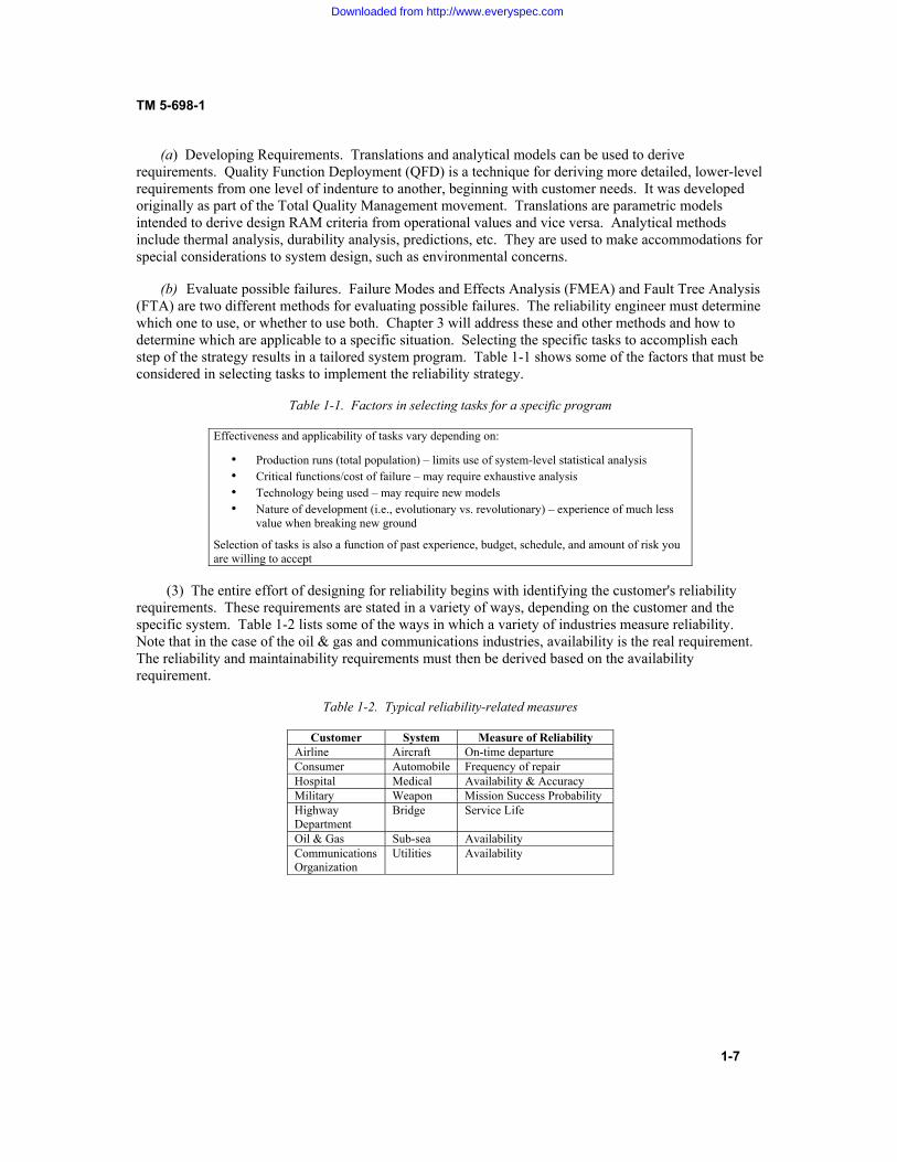
(a) Developing Requirements. Translations and analytical models can be used to derive requirements. Quality Function Deployment (QFD) is a technique for deriving more detailed, lower-level requirements from one level of indenture to another, beginning with customer needs. It was developed originally as part of the Total Quality Management movement. Translations are parametric models intended to derive design RAM criteria from operational values and vice versa. Analytical methods include thermal analysis, durability analysis, predictions, etc. They are used to make accommodations for special considerations to system design, such as environmental concerns. (b) Evaluate possible failures. Failure Modes and Effects Analysis (FMEA) and Fault Tree Analysis (FTA) are two different methods for evaluating possible failures. The reliability engineer must determine which one to use, or whether to use both. Chapter 3 will address these and other methods and how to determine which are applicable to a specific situation. Selecting the specific tasks to accomplish each step of the strategy results in a tailored system program. Table 1-1 shows some of the factors that must be considered in selecting tasks to implement the reliability strategy.

Table 1-1. Factors in selecting tasks for a specific program

Effectiveness and applicability of tasks vary depending on:

• Production runs (total population) – limits use of system-level statistical analysis • Critical functions/cost of failure – may require exhaustive analysis • Technology being used – may require new models • Nature of development (i.e., evolutionary vs. revolutionary) – experience of much less

value when breaking new ground

Selection of tasks is also a function of past experience, budget, schedule, and amount of risk you are willing to accept

(3) The entire effort of designing for reliability begins with identifying the customer's reliability requirements. These requirements are stated in a variety of ways, depending on the customer and the specific system. Table 1-2 lists some of the ways in which a variety of industries measure reliability. Note that in the case of the oil & gas and communications industries, availability is the real requirement. The reliability and maintainability requirements must then be derived based on the availability requirement.

Table 1-2. Typical reliability-related measures

Customer System Measure of Reliability Airline Aircraft On-time departure Consumer Automobile Frequency of repair Hospital Medical Availability & Accuracy Military Weapon Mission Success Probability Highway Department

Bridge Service Life

Oil & Gas Sub-sea Availability Communications Organization

Utilities Availability


TM 5-698-1

2-1

CHAPTER 2

BASIC RELIABILITY AND AVAILABILITY CONCEPTS

2-1. Probability and statistics This section provides the reader with an overview of the mathematics of reliability theory. It is not presented as a complete (or mathematically rigorous) discussion of probability theory and statistics, but should give the reader a reasonable understanding of how reliability is calculated. Before beginning the discussion, a key point must be made. Reliability is a design characteristic that indicates a system's ability to perform its mission over time without failure or without logistics support. In the first case, a failure can be defined as any incident that prevents the mission from being accomplished; in the second case, a failure is any incident requiring unscheduled maintenance. Reliability is achieved through sound design, the proper application of parts, and an understanding of failure mechanisms. Estimation and calculation techniques are necessary to help determine feasibility, assess progress, and provide failure probabilities and frequencies to spares calculations and other analyses. a. Uncertainty - at the heart of probability. The mathematics of reliability is based on probability theory. Probability theory, in turn, deals with uncertainty. The theory of probability had its origins in gambling. (1) Simple examples of probability in gambling are the odds against rolling a six on a die, of drawing a deuce from a deck of 52 cards, or of having a tossed coin come up heads. In each case, probability can be thought of as the relative frequency with which an event will occur in the long run. (a) When we assert that tossing an honest coin will result in heads (or tails) 50% of the time, we do not mean that we will necessarily toss five heads in ten trials. We only mean that in the long run, we would expect to see 50% heads and 50% tails. Another way to look at this example is to imagine a very large number of coins being tossed simultaneously; again, we would expect 50% heads and 50% tails. (b) When we have an honest die, we expect that the chance of rolling any possible outcome (one, two, three, four, five, or six) is one in six. Again, it is possible to roll a given number, say a six, several times in a row. However, in a large number of rolls, we would expect to roll a six (or a one, or a two, or a three, or a four, or a five) only 1/6 or 16.7% of the time. (c) If we draw from an honest deck of 52 cards, the chance of drawing a specific card (an ace, for example) is not as easily calculated as rolling a six with a die or tossing a heads with a coin. We must first recognize that there are four suits, each with a deuce through ace (ace being high). Therefore, there are four deuces, four tens, four kings, etc. So, if asked to draw an ace, we know that there are four aces and so the chance of drawing any ace is four in 52. We instinctively know that the chance of drawing the ace of spades, for example, is less than four in 52. Indeed, it is one in 52 (only one ace of spades in a deck of 52 cards). (2) Why is there a 50% chance of tossing a head on a given toss of a coin? It is because there are two results, or events, which can occur (assume that it is very unlikely for the coin to land on its edge) and for a balanced, honest coin, there is no reason for either event to be favored. Thus, we say the outcome is random and each event is equally likely to occur. Hence, the probability of tossing a head (or tail) is one of two equally probable events occurring = 1/2 = 0.5 = 50% of the time. On the other hand,


TM 5-698-1

2-2

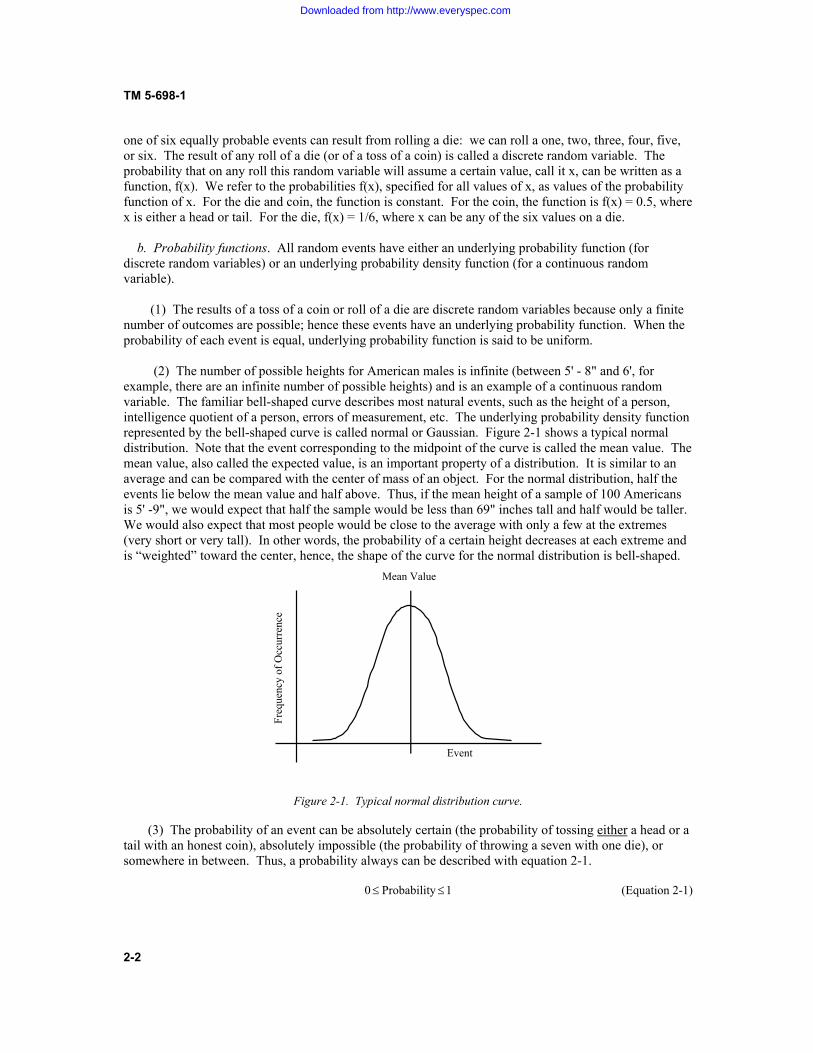
one of six equally probable events can result from rolling a die: we can roll a one, two, three, four, five, or six. The result of any roll of a die (or of a toss of a coin) is called a discrete random variable. The probability that on any roll this random variable will assume a certain value, call it x, can be written as a function, f(x). We refer to the probabilities f(x), specified for all values of x, as values of the probability function of x. For the die and coin, the function is constant. For the coin, the function is f(x) = 0.5, where x is either a head or tail. For the die, f(x) = 1/6, where x can be any of the six values on a die. b. Probability functions. All random events have either an underlying probability function (for discrete random variables) or an underlying probability density function (for a continuous random variable). (1) The results of a toss of a coin or roll of a die are discrete random variables because only a finite number of outcomes are possible; hence these events have an underlying probability function. When the probability of each event is equal, underlying probability function is said to be uniform. (2) The number of possible heights for American males is infinite (between 5' - 8" and 6', for example, there are an infinite number of possible heights) and is an example of a continuous random variable. The familiar bell-shaped curve describes most natural events, such as the height of a person, intelligence quotient of a person, errors of measurement, etc. The underlying probability density function represented by the bell-shaped curve is called normal or Gaussian. Figure 2-1 shows a typical normal distribution. Note that the event corresponding to the midpoint of the curve is called the mean value. The mean value, also called the expected value, is an important property of a distribution. It is similar to an average and can be compared with the center of mass of an object. For the normal distribution, half the events lie below the mean value and half above. Thus, if the mean height of a sample of 100 Americans is 5' -9", we would expect that half the sample would be less than 69" inches tall and half would be taller. We would also expect that most people would be close to the average with only a few at the extremes (very short or very tall). In other words, the probability of a certain height decreases at each extreme and is “weighted” toward the center, hence, the shape of the curve for the normal distribution is bell-shaped.

Figure 2-1. Typical normal distribution curve. (3) The probability of an event can be absolutely certain (the probability of tossing either a head or a tail with an honest coin), absolutely impossible (the probability of throwing a seven with one die), or somewhere in between. Thus, a probability always can be described with equation 2-1. 1 y Probabilit 0 dd (Equation 2-1)

Event

Mean Value

Freq

uenc

y of

Occ

urre

nce


TM 5-698-1

2-3

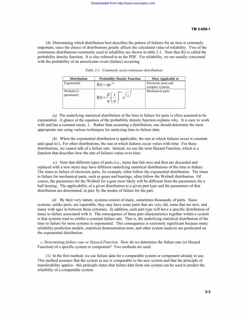
(4) Determining which distribution best describes the pattern of failures for an item is extremely important, since the choice of distributions greatly affects the calculated value of reliability. Two of the continuous distributions commonly used in reliability are shown in table 2-1. Note that f(t) is called the probability density function. It is also referred to as the PDF. For reliability, we are usually concerned with the probability of an unwelcome event (failure) occurring.

Table 2-1. Commonly used continuous distributions

Distribution Probability Density Function Most Applicable to Exponential t-f(t) OKe Electronic parts and

complex systems Weibull (2-parameter)

E

KE

KKE ¸̧

¹

·¨̈©

§

¸̧¹

·¨̈©

§

t-1-

t f(t) e

Mechanical parts

(a) The underlying statistical distribution of the time to failure for parts is often assumed to be exponential. A glance at the equation of the probability density function explains why. It is easy to work with and has a constant mean, O . Rather than assuming a distribution, one should determine the most appropriate one using various techniques for analyzing time-to-failure data. (b) When the exponential distribution is applicable, the rate at which failures occur is constant and equal to O� For other distributions, the rate at which failures occur varies with time. For these distributions, we cannot talk of a failure rate. Instead, we use the term Hazard Function, which is a function that describes how the rate of failures varies over time. (c) Note that different types of parts (i.e., items that fail once and then are discarded and replaced with a new item) may have different underlying statistical distributions of the time to failure. The times to failure of electronic parts, for example, often follow the exponential distribution. The times to failure for mechanical parts, such as gears and bearings, often follow the Weibull distribution. Of course, the parameters for the Weibull for a gear most likely will be different from the parameters for a ball bearing. The applicability of a given distribution to a given part type and the parameters of that distribution are determined, in part, by the modes of failure for the part. (d) By their very nature, systems consist of many, sometimes thousands, of parts. Since systems, unlike parts, are repairable, they may have some parts that are very old, some that are new, and many with ages in between these extremes. In addition, each part type will have a specific distribution of times to failure associated with it. The consequence of these part characteristics together within a system is that systems tend to exhibit a constant failure rate. That is, the underlying statistical distribution of the time to failure for most systems is exponential. This consequence is extremely significant because many reliability prediction models, statistical demonstration tests, and other system analysis are predicated on the exponential distribution. c. Determining failure rate or Hazard Function. How do we determine the failure rate (or Hazard Function) of a specific system or component? Two methods are used. (1) In the first method, we use failure data for a comparable system or component already in use. This method assumes that the system in use is comparable to the new system and that the principle of transferability applies - this principle states that failure data from one system can be used to predict the reliability of a comparable system.


TM 5-698-1

2-4

(2) The other method of determining failure rate or the Hazard Function is through testing of the system or its components. Although, theoretically, this method should be the "best" one, it has two disadvantages. First, predictions are needed long before prototypes or pre-production versions of the system are available for testing. Second, the reliability of some components is so high that the cost of testing to measure the reliability in a statistically valid manner would be prohibitive. Usually, failure data from comparable systems are used in the early development phases of a new system and supplemented with test data when available. 2-2. Calculating reliability If the time (t) over which a system must operate and the underlying distributions of failures for its constituent elements are known, then the system reliability can be calculated by taking the integral (essentially the area under the curve defined by the PDF) of the PDF from t to infinity, as shown in equation 2-2.

³f t dt f(t) R(t) (Equation 2-2)

a. Exponential distribution. If the underlying failure distribution is exponential, equation 2-2 becomes equation 2-3.

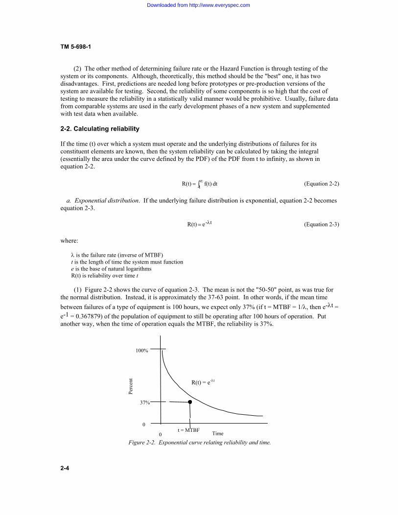
t-e R(t) O (Equation 2-3) where: O�is the failure rate (inverse of MTBF) t is the length of time the system must function e is the base of natural logarithms R(t) is reliability over time t (1) Figure 2-2 shows the curve of equation 2-3. The mean is not the "50-50" point, as was true for the normal distribution. Instead, it is approximately the 37-63 point. In other words, if the mean time between failures of a type of equipment is 100 hours, we expect only 37% (if t = MTBF = 1/O, then e-Ot = e-1 = 0.367879) of the population of equipment to still be operating after 100 hours of operation. Put another way, when the time of operation equals the MTBF, the reliability is 37%.

Figure 2-2. Exponential curve relating reliability and time. Time

100%

0 0

t = MTBF

37% R(t) = e-Ot

�

Perc

ent


TM 5-698-1

2-5

(2) If the underlying distribution for each element is exponential and the failure rates (Oi) for each element are known, then the reliability of the system can be calculated using equation 2-3. b. Series Reliability. Consider the system represented by the reliability block diagram (RBD) in figure 2-3.

1. The number above each block is the failure rate in failures per million hours. The inverse of the failure rate is the mean time to failure (exponential failure rate assumed). 2. The number below each block is the reliability calculated using equation 2-3 with t = 10 hours.

Figure 2-3. Example reliability block diagram.

(1) Components A and B in figure 2-3 are said to be in series, which means all must operate for the system to operate. Since the system can be no more reliable than the least reliable component, this configuration is often referred to as the weakest link configuration. (2) Since the components are in series, the system reliability can be found by adding together the failure rates of the components and substituting the result as seen in equation 2-4. Furthermore, if the individual reliabilities are calculated (the bottom values,) we could find the system reliability by multiplying the reliabilities of the two components as shown in equation 2-4a. 9753.0)( 100025.0)( �� xt eetR BA OO (Equation 2-4)

9753.098510.099000.0)()()( u u tRtRtR BA (Equation 2-4a) c. Reliability with Redundancy. Now consider the RBD shown in figure 2-4.

1. Each block represents the series configuration of components A and B. 2. The number below each block is the reliability calculated using equations 2-3 and 2-4 with t = 10 hours.

Figure 2-4. RBD of a system with redundant components. (1) The system represented by the RBD in figure 2-4 has the same components (A and B in series denoted by one block labeled: A-B) used in figure 2-3, but two of each component are used in a configuration referred to as redundant or parallel. Two paths of operation are possible. The paths are: top A-B and bottom A-B. If either of two paths is intact, the system can operate. The reliability of the system is most easily calculated by (equation 2-5) finding the probability of failure (1 - R(t)) for each

A B 0.00100 0.00150

0.99005 0.98511

A-B

A-B

0.9753

0.9753


TM 5-698-1

2-6

path, multiplying the probabilities of failure (which gives the probability of both paths failing), and then subtracting the result from 1. The reliability of each path was found in the previous example. Next, the probability of a path failing is found by subtracting its reliability from 1. Thus, the probability of either path failing is 1 - 0.9753 = 0.0247. The probability that both paths will fail is 0.0247 x 0.0247 = 0.0006. Finally, the reliability of the system is 1 - 0.0006 = 0.9994, about a 2.5% improvement over the series-configured system. 9994.0)0274.00274.0(1))(1())(1(1)( u� �u�� tRtRtR BT (Equation 2-5) where: RT is the reliability of the top path RB is the reliability of the bottom path (2) Two components in parallel may always be on and in operation (active redundancy) or one may be off (standby redundancy). In the latter case, failure of the primary component must be sensed to indicate that the standby module should be activated. Standby redundancy may be necessary to avoid interference between the redundant components. If the redundant component is normally off, reduces the time over which the redundant component will be used (it's only used from the time when the primary component fails. Of course, more than two components can be in parallel. Chapter 3 discusses the various types of redundancy and how they can be used to improve the availability of current C4ISR facilities. (3) Adding a component in parallel, i.e., redundancy, improves the system's ability to perform its function. This aspect of reliability is called functional or mission reliability. Note, however, that in figure 2-4, we have added another set of components that has its own failure rate. If we want to calculate the total failure rate for all components, we add them. The result is 5000 failures per million operating hours (0.005000). The failure rate for the series-configured system in figure 2-3 was 2500 failures per million operating hours. Although the functional reliability of the system improved, the total failure rate for all components increased. This perspective of reliability is called basic or logistics reliability. When standby redundancy is used, the sensing and switching components add to the total failure rate. d. Logistics reliability. Whereas functional reliability only considers failures of the function(s), logistics reliability considers all failures because some maintenance action will be required. Logistics reliability can be considered as either the lack of demand placed on the logistics system by failures or the ability to operate without logistics. If standby redundancy is used with the redundant component not on, the apparent failure rate of the standby component will be less than that of its counterpart (it will likely operate less than ten hours), but the failure rate of the switching circuits must now be considered. 2-3. Calculating availability For a system such as an electrical power system, availability is a key measure of performance. An electrical power facility must operate for very long periods of time, providing power to systems that perform critical functions, such as C4ISR. Even with the best technology and most robust design, it is economically impractical, if not technically impossible, to design power facilities that never fail over weeks or months of operation. Although forced outages (FAs) are never welcome and power facilities are designed to minimize the number of FAs, they still occur. When they do, restoring the system to operation as quickly and economically as possible is paramount. The maintainability characteristics of the system predict how quickly and economically system operation can be restored. a. Reliability, availability, and maintainability. Reliability and maintainability (R&M) are considered complementary characteristics. Looking at a graph of constant curves of inherent availability (Ai), one


TM 5-698-1

2-7

can see this complementary relationship. Ai is defined by the following equation and reflects the percent of time a system would be available if delays due to maintenance, supply, etc. are ignored.

%100 xMTTRMTBF

MTBFAi � (Equation 2-6)

where MTBF is mean time between failure and MTTR is mean time to repair As seen in equation 2-6, if the system never failed, the MTBF would be infinite and Ai would be 100%. Or, if it took no time at all to repair the system, MTTR would be zero and again the availability would be 100%. Figure 2-5 is a graph showing availability as a function of reliability and maintainability (availability is calculated using equation 2-6). Note that you can achieve the same availability with different values of R&M. With higher reliability (MTBF), lower levels of maintainability are needed to achieve the same availability and vice versa. It is very common to limit MTBF, MTTR, or both. For example, the availability requirement might be 95% with an MTBF of at least 600 hours and a MTTR of no more than 3.5 hours.

Figure 2-5. Different combinations of MTBF and MTTR yield the same availability. b. Other measures of availability. Availability is calculated through data collection by two primary methods: (1) Operational availability includes maintenance and logistics delays and is defined using equation 2-7:

MDTMTBM

MTBM A0 � (Equation 2-7)

where MTBM is the mean time between all maintenance and MDT is the mean downtime for each maintenance action.

0 10 20 30 40 50 60 70 80 90 100 65

70

75

80

85

90

95

100

MEAN TIME TO REPAIR (HOURS)

AV

AIL

AB

ILIT

Y

(PER

CEN

T)

MTBF = 1000

MTBF = 800 MTBF = 600

MTBF = 400

MTBF = 200


TM 5-698-1

2-8

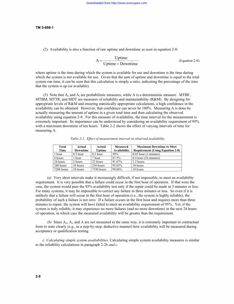
(2) Availability is also a function of raw uptime and downtime as seen in equation 2-8:

Downtime Uptime

Uptime A �

(Equation 2-8)

where uptime is the time during which the system is available for use and downtime is the time during which the system is not available for use. Given that the sum of uptime and downtime is equal to the total system run time, it can be seen that this calculation is simply a ratio, indicating the percentage of the time that the system is up (or available). (3) Note that Ao and Ai are probabilistic measures, while A is a deterministic measure. MTBF, MTBM, MTTR, and MDT are measures of reliability and maintainability (R&M). By designing for appropriate levels of R&M and ensuring statistically appropriate calculations, a high confidence in the availability can be obtained. However, that confidence can never be 100%. Measuring A is done by actually measuring the amount of uptime in a given total time and then calculating the observed availability using equation 2-8. For this measure of availability, the time interval for the measurement is extremely important. Its importance can be understood by considering an availability requirement of 95% with a maximum downtime of ten hours. Table 2-2 shows the effect of varying intervals of time for measuring A.

Table 2-2. Effect of measurement interval on observed availability

Total Time

Actual Downtime

Actual Uptime

Measured Availability

Maximum Downtime to Meet Requirement (Using Equation 2-8)

1 hour 0.5 hour 0.5 hour 50% 0.05 hour (3 minutes) 8 hours 1 hour 7 hour 87.5% 0.4 hour (24 minutes) 24 hours 2 hours 22 hours 91.67% 1.2 hours 240 hours 10 hours 230 hours 95.83% 10 hours 7200 hours 10 hours 7190 hours 99.86% 10 hours

(a) Very short intervals make it increasingly difficult, if not impossible, to meet an availability requirement. It is very possible that a failure could occur in the first hour of operation. If that were the case, the system would pass the 95% availability test only if the repair could be made in 3 minutes or less. For many systems, it may be impossible to correct any failure in three minutes or less. So even if it is unlikely that a failure will occur in the first hour of operation (i.e., the system is highly reliable), the probability of such a failure is not zero. If a failure occurs in the first hour and requires more than three minutes to repair, the system will have failed to meet an availability requirement of 95%. Yet, if the system is truly reliable, it may experience no more failures (and no more downtime) in the next 24 hours of operation, in which case the measured availability will be greater than the requirement. (b) Since Ao, Ai, and A are not measured in the same way, it is extremely important in contractual form to state clearly (e.g., in a step-by-step, deductive manner) how availability will be measured during acceptance or qualification testing. c. Calculating simple system availabilities. Calculating simple system availability measures is similar to the reliability calculations in paragraph 2-2b and c.


TM 5-698-1

2-9

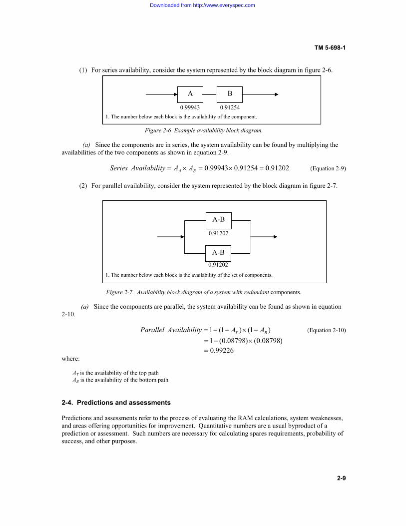
(1) For series availability, consider the system represented by the block diagram in figure 2-6.

1. The number below each block is the availability of the component.

Figure 2-6 Example availability block diagram. (a) Since the components are in series, the system availability can be found by multiplying the availabilities of the two components as shown in equation 2-9. 91202.091254.099943.0 u u BA AAtyAvailabiliSeries (Equation 2-9) (2) For parallel availability, consider the system represented by the block diagram in figure 2-7.

1. The number below each block is the availability of the set of components.

Figure 2-7. Availability block diagram of a system with redundant components. (a) Since the components are parallel, the system availability can be found as shown in equation 2-10. )1()1(1 BT AAtyAvailabiliParallel �u�� (Equation 2-10)

)08798.0()08798.0(1 u� 99226.0 where: AT is the availability of the top path AB is the availability of the bottom path 2-4. Predictions and assessments Predictions and assessments refer to the process of evaluating the RAM calculations, system weaknesses, and areas offering opportunities for improvement. Quantitative numbers are a usual byproduct of a prediction or assessment. Such numbers are necessary for calculating spares requirements, probability of success, and other purposes.

A B

0.99943 0.91254

A-B

A-B

0.91202

0.91202


TM 5-698-1

2-10

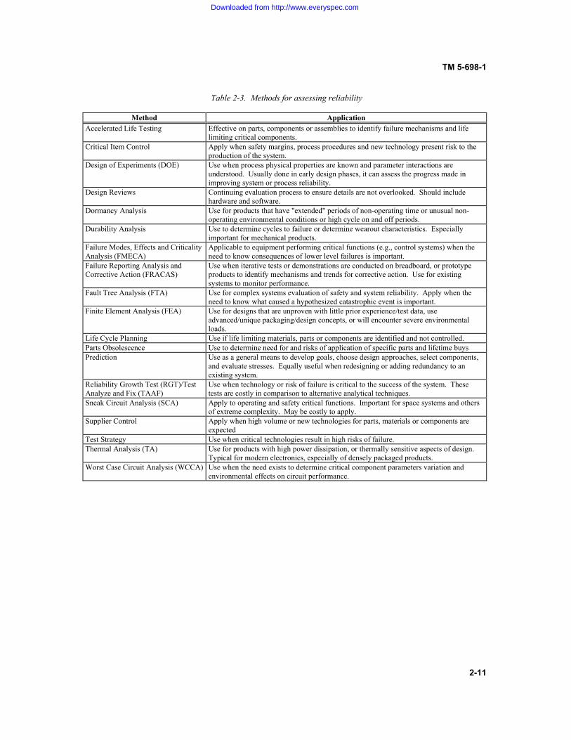
a. Reliability Predictions. In a new development program, reliability predictions are a means of determining the feasibility of requirements, assessing progress toward achieving those requirements, and comparing the reliability impact of design alternatives. Predictions can be made through any appropriate combination of reliability models, historical data, test data, and engineering judgment. The choice of which prediction method to use depends on the availability of information. That choice can also be a function of the point of the system life cycle at which the prediction is performed. Considerations in performing predictions include: that correct environmental stresses are used, the reliability model is correct, the correct part qualities are assumed, and that all operational and dormancy modes are reflected. Chapter 4 addresses the types of modeling methods commonly used. b. Reliability Assessment. Predictions are one method of assessing the reliability of an item. At the onset of a new development program, the prediction is usually purely analytical. As the program progresses, other methods become available to improve or augment the analytical prediction. These methods include testing, design reviews, and others. For existing systems, reliability assessments include analyzing field data to determine the level of reliability being achieved and identify weaknesses in the design and opportunities for improvement. (1) Table 2-3 lists some common techniques that can be used for assessing reliability and guidance for their use. Some of these methods provide a numerical value that is representative of the system reliability at a point in time; all provide a valuable means of better understanding the design's strengths and weaknesses so that it can be changed accordingly. (2) The assessment methods chosen should be appropriate for the system and require only a reasonable level of investment given the value of the results. The failure of some components, for example, may have little impact on either system function, or on its operating and repair costs. A relatively costly analysis may not be justified. For other systems, a thermal analysis may not be needed, given the nature of the system and its operating environment. When the consequences of failure are catastrophic, every possible effort should be made to make the system fail-safe or fault-tolerant.


TM 5-698-1

2-11

Table 2-3. Methods for assessing reliability

Method Application Accelerated Life Testing Effective on parts, components or assemblies to identify failure mechanisms and life

limiting critical components. Critical Item Control Apply when safety margins, process procedures and new technology present risk to the

production of the system. Design of Experiments (DOE) Use when process physical properties are known and parameter interactions are

understood. Usually done in early design phases, it can assess the progress made in improving system or process reliability.

Design Reviews Continuing evaluation process to ensure details are not overlooked. Should include hardware and software.

Dormancy Analysis

Use for products that have "extended" periods of non-operating time or unusual non-operating environmental conditions or high cycle on and off periods.

Durability Analysis Use to determine cycles to failure or determine wearout characteristics. Especially important for mechanical products.

Failure Modes, Effects and Criticality Analysis (FMECA)

Applicable to equipment performing critical functions (e.g., control systems) when the need to know consequences of lower level failures is important.

Failure Reporting Analysis and Corrective Action (FRACAS)

Use when iterative tests or demonstrations are conducted on breadboard, or prototype products to identify mechanisms and trends for corrective action. Use for existing systems to monitor performance.

Fault Tree Analysis (FTA) Use for complex systems evaluation of safety and system reliability. Apply when the need to know what caused a hypothesized catastrophic event is important.

Finite Element Analysis (FEA) Use for designs that are unproven with little prior experience/test data, use advanced/unique packaging/design concepts, or will encounter severe environmental loads.

Life Cycle Planning Use if life limiting materials, parts or components are identified and not controlled. Parts Obsolescence Use to determine need for and risks of application of specific parts and lifetime buys Prediction Use as a general means to develop goals, choose design approaches, select components,

and evaluate stresses. Equally useful when redesigning or adding redundancy to an existing system.

Reliability Growth Test (RGT)/Test Analyze and Fix (TAAF)

Use when technology or risk of failure is critical to the success of the system. These tests are costly in comparison to alternative analytical techniques.

Sneak Circuit Analysis (SCA) Apply to operating and safety critical functions. Important for space systems and others of extreme complexity. May be costly to apply.

Supplier Control Apply when high volume or new technologies for parts, materials or components are expected

Test Strategy Use when critical technologies result in high risks of failure. Thermal Analysis (TA) Use for products with high power dissipation, or thermally sensitive aspects of design.

Typical for modern electronics, especially of densely packaged products. Worst Case Circuit Analysis (WCCA) Use when the need exists to determine critical component parameters variation and

environmental effects on circuit performance.


TM 5-698-1

3-1

CHAPTER 3

IMPROVING AVAILABILITY OF C4ISR FACILITIES

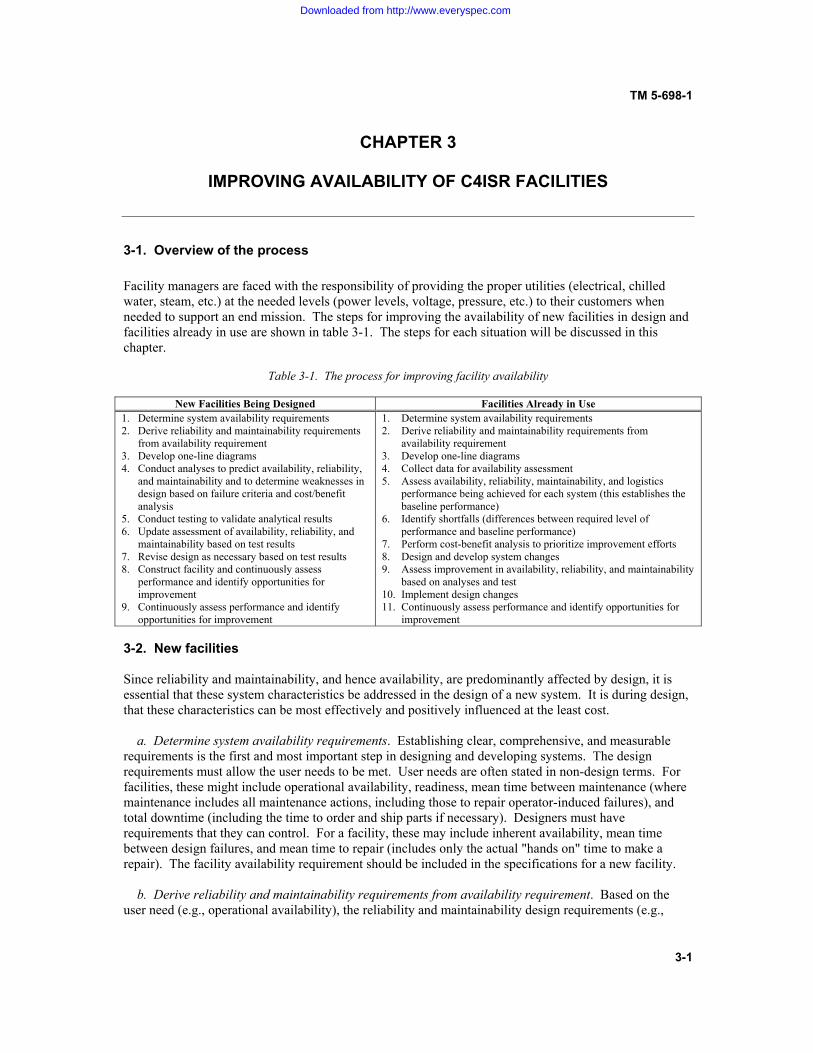
3-1. Overview of the process Facility managers are faced with the responsibility of providing the proper utilities (electrical, chilled water, steam, etc.) at the needed levels (power levels, voltage, pressure, etc.) to their customers when needed to support an end mission. The steps for improving the availability of new facilities in design and facilities already in use are shown in table 3-1. The steps for each situation will be discussed in this chapter.

Table 3-1. The process for improving facility availability

New Facilities Being Designed Facilities Already in Use

1. Determine system availability requirements 2. Derive reliability and maintainability requirements

from availability requirement 3. Develop one-line diagrams 4. Conduct analyses to predict availability, reliability,

and maintainability and to determine weaknesses in design based on failure criteria and cost/benefit analysis

5. Conduct testing to validate analytical results 6. Update assessment of availability, reliability, and

maintainability based on test results 7. Revise design as necessary based on test results 8. Construct facility and continuously assess

performance and identify opportunities for improvement

9. Continuously assess performance and identify opportunities for improvement

1. Determine system availability requirements 2. Derive reliability and maintainability requirements from

availability requirement 3. Develop one-line diagrams 4. Collect data for availability assessment 5. Assess availability, reliability, maintainability, and logistics

performance being achieved for each system (this establishes the baseline performance)

6. Identify shortfalls (differences between required level of performance and baseline performance)

7. Perform cost-benefit analysis to prioritize improvement efforts 8. Design and develop system changes 9. Assess improvement in availability, reliability, and maintainability

based on analyses and test 10. Implement design changes 11. Continuously assess performance and identify opportunities for

improvement 3-2. New facilities Since reliability and maintainability, and hence availability, are predominantly affected by design, it is essential that these system characteristics be addressed in the design of a new system. It is during design, that these characteristics can be most effectively and positively influenced at the least cost. a. Determine system availability requirements. Establishing clear, comprehensive, and measurable requirements is the first and most important step in designing and developing systems. The design requirements must allow the user needs to be met. User needs are often stated in non-design terms. For facilities, these might include operational availability, readiness, mean time between maintenance (where maintenance includes all maintenance actions, including those to repair operator-induced failures), and total downtime (including the time to order and ship parts if necessary). Designers must have requirements that they can control. For a facility, these may include inherent availability, mean time between design failures, and mean time to repair (includes only the actual "hands on" time to make a repair). The facility availability requirement should be included in the specifications for a new facility. b. Derive reliability and maintainability requirements from availability requirement. Based on the user need (e.g., operational availability), the reliability and maintainability design requirements (e.g.,


TM 5-698-1

3-2

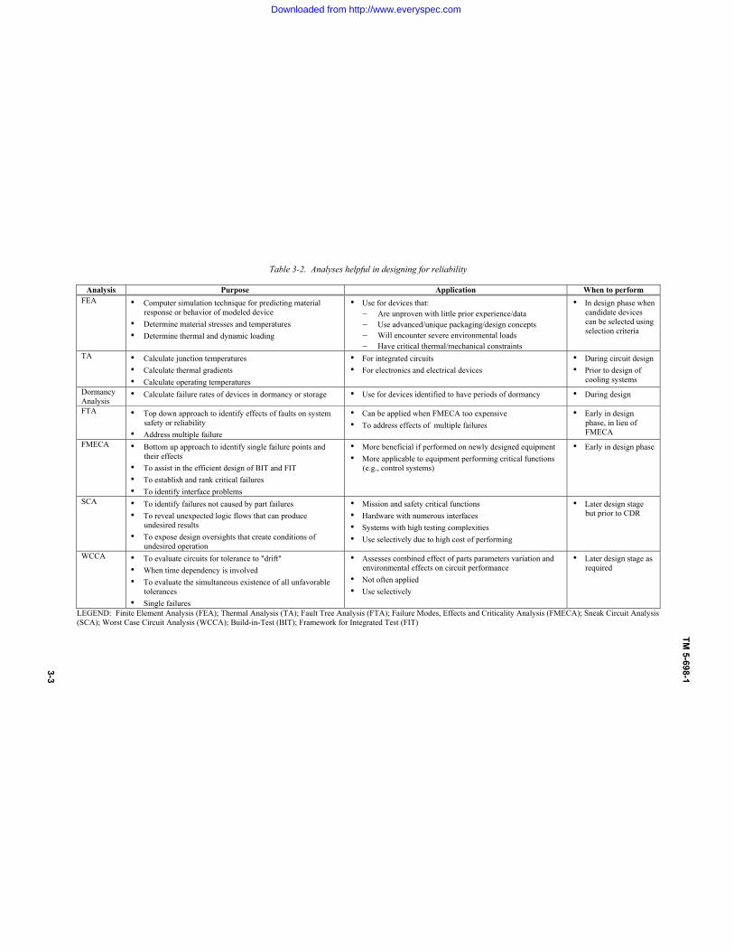
mean time between failure and mean time to repair) must be derived. This derivation of lower-level requirements is usually done by the design organization and continues throughout the development effort until design requirements are available at the lowest level of indenture (subsystem, assembly, subassembly, part) that makes sense. c. Develop one-line diagrams. One line diagrams will be instrumental in the creation of all models concerning RAM criteria and analysis. It is critical that diagrams are accurate and up-to-date. Paragraph 4-5 of this manual demonstrates how one-line diagrams are used in modeling and calculation. d. Conduct Analyses. Conduct analyses to predict availability, reliability, and maintainability and to determine weaknesses in design and redesign based on failure criteria and cost/benefit analysis. Some of the pertinent analyses are summarized in table 3-2. e. Conduct testing to validate analytical results. No matter how diligent we are in developing the models and analytical tools used to design, we cannot account for all variations and factors. By testing a given design, we will uncover unexpected problems. These problems can include new types of failures, more frequent than expected failures, different effects of failures, and so forth. Problems discovered during test provide opportunities for improving the design and our models and tools.

f. Update assessment of availability, reliability, and maintainability based on test results. Based on the results of our testing, we should update the analytical assessments of reliability made earlier. Adding the results of testing provides higher confidence in our assessment than is possible using analytical results alone. g. Revise design as necessary based on test results. If our updated assessment indicates we are falling short of our RAM requirements, we must revise the design to improve the reliability. Even when our updated assessment indicates that we are or are close to meeting our requirements, we should consider making design changes referencing cost-benefit considerations. h. Construct facility and continuously assess performance and identify opportunities for improvement. Once we are satisfied that the RAM requirements are satisfied by our facility design, the facility is constructed. We must ensure that the inherent levels of reliability are sustained over time, and collect information that can be used in the design of the next facility. To that end, we need to collect and use data to continuously assess the availability performance of the facility. This operational, field data also should be archived for use in designing new facilities.


3-3

TM 5-698-1

Table 3-2. Analyses helpful in designing for reliability

Analysis Purpose Application When to perform FEA • Computer simulation technique for predicting material

response or behavior of modeled device • Determine material stresses and temperatures • Determine thermal and dynamic loading

• Use for devices that: � Are unproven with little prior experience/data � Use advanced/unique packaging/design concepts � Will encounter severe environmental loads � Have critical thermal/mechanical constraints

• In design phase when candidate devices can be selected using selection criteria

TA • Calculate junction temperatures • Calculate thermal gradients • Calculate operating temperatures

• For integrated circuits • For electronics and electrical devices

• During circuit design • Prior to design of

cooling systems Dormancy Analysis

• Calculate failure rates of devices in dormancy or storage • Use for devices identified to have periods of dormancy • During design

FTA

• Top down approach to identify effects of faults on system safety or reliability

• Address multiple failure

• Can be applied when FMECA too expensive • To address effects of multiple failures

• Early in design phase, in lieu of FMECA

FMECA • Bottom up approach to identify single failure points and their effects

• To assist in the efficient design of BIT and FIT • To establish and rank critical failures • To identify interface problems

• More beneficial if performed on newly designed equipment • More applicable to equipment performing critical functions

(e.g., control systems)

• Early in design phase

SCA • To identify failures not caused by part failures • To reveal unexpected logic flows that can produce

undesired results • To expose design oversights that create conditions of

undesired operation

• Mission and safety critical functions • Hardware with numerous interfaces • Systems with high testing complexities • Use selectively due to high cost of performing

• Later design stage but prior to CDR

WCCA • To evaluate circuits for tolerance to "drift" • When time dependency is involved • To evaluate the simultaneous existence of all unfavorable

tolerances • Single failures

• Assesses combined effect of parts parameters variation and environmental effects on circuit performance

• Not often applied • Use selectively

• Later design stage as required

LEGEND: Finite Element Analysis (FEA); Thermal Analysis (TA); Fault Tree Analysis (FTA); Failure Modes, Effects and Criticality Analysis (FMECA); Sneak Circuit Analysis (SCA); Worst Case Circuit Analysis (WCCA); Build-in-Test (BIT); Framework for Integrated Test (FIT)


TM 5-698-1

3-4

3-3. Existing facilities For facilities in use, the process for improving availability is somewhat different than that discussed for new systems. It is different for two major reasons. First, improvements must be made by modifying an existing design, which is usually more difficult than creating the original design. Second, the improvements must be made with as little disruption to the facility as possible, since it is supporting an ongoing mission. Although design changes are usually the primary focus of improvement efforts, changes in procedures or policy should also be considered. Not only are such changes usually much easier and economical to make, they may actually be more effective in increasing availability. a. Determine system availability requirements. As was the case for a new system, the requirements must be known. For existing facilities, it may be difficult to find the original user needs or design requirements. Even when the original requirements can be determined, the current requirements may have changed due to mission changes, budget constraints, or other factors. b. Derive reliability and maintainability requirements from the availability requirement. After the system availability requirements are determined, it is necessary to translate them into reliability and maintainability requirements. c. Develop one-line diagrams. This step can be bypassed if original one-lines are still current. d. Collect data for availability assessment. Ideally, a data collection system was implemented when the facility was first put into operation. If that is not the case, one should be developed and implemented. The data to be collected includes the category of failures, causes of failures, date and time when failures occur, mechanisms affected, and so on. A substantial byproduct of an RCM program is the generation of such unique, facility data. e. Assess performance. Assess the availability, reliability, maintainability, and logistics performance being achieved for each system. Performing this step establishes the baseline performance for the facility. f. Identify shortfalls. Shortfalls are the differences between the required level of performance and baseline performance. g. Perform cost-benefit analysis to prioritize improvement efforts. Many potential improvements will be identified throughout the life of a facility. Those that are safety-related or are essential for mission success will always be given the highest priority. Others will be prioritized on the basis of the costs to implement compared with the projected benefits. Those that have only a small return for the investment will be given the lowest priority. h. Design and develop system changes. The process for improving the availability, reliability, and maintainability performance of an existing facility is essentially the same as for designing new facility. i. Assess improvement. Assess improvement in reliability, availability, and maintainability based on analyses and tests. Before implementing any potential improvements, some effort must be made to ensure that the design changes must be validated. All too often, a change that was intended to improve the situation actually makes it worse. Through careful analyses and


TM 5-698-1

3-5

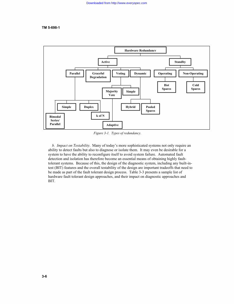
appropriate testing, one can determine that the proposed change actually results in some level of improvement. j. Implement design changes. Those design changes that are validated as improving availability must be implemented in a way that minimizes the downtime of the facility. Perhaps they can be made during scheduled maintenance periods. Or perhaps there are times of the day, month, or year when downtime is less critical to the mission than at other times. Careful planning can minimize the impact on the mission. Also, the procedures, tools, training, and materials needed for the design change must be in place and validated prior to starting the facility modification. k. Monitor performance. Continuously assess performance and identify opportunities for improvement. Continuous improvement should be the goal of every facility manager. As the facility ages, the cost-benefits of what were low-priority improvements may change, new problems may be introduced, and new mission requirements may arise. By collecting data and maintaining a baseline of the facility availability performance, the facility manager will be in a position to make future improvements as they become necessary or economical. 3-4. Improving availability through addition of redundancy Redundancy is a technique for increasing system reliability and availability by making the system immune to the failure of a single component. It is a form of fault tolerance – the system can tolerate one or more component failures and still perform its function(s). a. Types of Redundancy. There are essentially two kinds of redundancy techniques employed in fault tolerant designs, space redundancy and time redundancy. Space redundancy provides separate physical copies of a resource, function, or data item. Time redundancy, used primarily in digital systems, involves the process of storing information to handle transients, or encoding information that is shifted in time to check for unwanted changes. Space, or hardware, redundancy is the approach most commonly associated with fault tolerant design. Figure 3-1 provides a simplified tree-structure showing the various types of hardware redundancy that have been used or considered in the past.


TM 5-698-1

3-6

Figure 3-1. Types of redundancy.

b. Impact on Testability. Many of today’s more sophisticated systems not only require an ability to detect faults but also to diagnose or isolate them. It may even be desirable for a system to have the ability to reconfigure itself to avoid system failure. Automated fault detection and isolation has therefore become an essential means of obtaining highly fault-tolerant systems. Because of this, the design of the diagnostic system, including any built-in-test (BIT) features and the overall testability of the design are important tradeoffs that need to be made as part of the fault tolerant design process. Table 3-3 presents a sample list of hardware fault tolerant design approaches, and their impact on diagnostic approaches and BIT.

Hardware Redundancy

Active Standby

Graceful Degradation

Voting Dynamic Operating Non-Operating Parallel

k of N

Simple Duplex

Majority Vote

Simple

Hybrid Pooled Spares

Bimodal Series/

Parallel Adaptive

Cold Spares

Hot Spares


TM 5-698-1

3-7

Table 3-3. Diagnostic implications of fault tolerant design approaches

(1) No matter which technique is chosen to implement fault tolerance in a design, the ability to achieve fault tolerance is becoming increasingly dependent on the ability to detect, and isolate malfunctions as they occur or are anticipated to occur. Alternate maintainability diagnostic concepts must be carefully reviewed for effectiveness before committing to a final design approach. In particular, BIT design has become very important to achieving a fault tolerant system. When using BIT in fault tolerant system design, the BIT system must do the following:

(a) Maintain real-time status of the system’s assets (on-line and off-line, or standby, equipment). (b) Provide the operator with the status of available system assets.

(c) Maintain a record of hardware faults for post-mission evaluation and corrective maintenance.

Fault Tolerant Design

Technique Description Diagnostic Design Implications BIT Implications

Active Redundancy, simple parallel

All parallel units are on whenever the system is operating. k of the N units are needed, where 0<k<N. External components are not required to perform the function of detection, decision and switching when an element or path in the structure fails. Since the redundant units are always operating, they automatically pick up the load for a failed unit. An example is a multi-engined aircraft. The aircraft can continue to fly with one or more engines out of operation.

Hardware/Software is more readily available to perform multiple functions.

N/A

Active Redundancy with voting logic

Same as Active Redundancy but where a majority of units must agree (for example, when multiple computers are used)

Performance/status-monitoring function assures the operator that the equipment is working properly; failure is more easily isolated to the locked-out branch by the voting logic.

N/A

Stand-by redundancy (Non-operating)

The redundant units are not operating and must be started if a failure is detected in the active unit (e.g., a spare radio is turned on when the primary radio fails).

Test capability and diagnostic functions must be designed into each redundant or substitute functional path (on-line AND off-line) to determine their status.

Passive, periodic, or manually initiated BIT.

Stand-by redundancy (Operating)

The redundant units are operating but not active in system operation; must be switched “in” if a failure is detected in the active unit (e.g., a redundant radar transmitter feeding a dummy load is switched into the antenna when the main transmitter fails).

N/A Limited to passive BIT (i.e., continuous monitoring) supplemented with periodic BIT.


TM 5-698-1

3-8

(2) The essence of fault tolerance is that the system is able to perform its mission despite experiencing some failures. In systems where redundancy is used, this fault tolerance is achieved by one or more redundant units taking over the function previously being performed by another unit. When standby redundancy is used, the failed unit must be detected and the standby unit “brought online.” In still other cases principally involving electronics, failures can be repaired by rerouting signals or functions to other units. These repairs can be done upon a failure or in anticipation of a failure. In such cases, the BIT should, in addition to the actions identified in paragraph 3-4b; maintain a record of any reconfiguration events that were required for system recovery during the mission. (3) For fault tolerant systems, it is important that the design’s inherent testability provisions include the ability to detect, identify, recover, and if possible reconfigure, and report equipment malfunctions to operational personnel. The reliability block diagrams for fault tolerant systems are complex, with non-serial connections. Fault tolerant systems often have a multitude of backups with non-zero switch-over time and imperfect fault detection, isolation, and recovery. Therefore, it is imperative that effective testability provisions be incorporated in the system design concept. If they are not, the fielded design will exhibit long troubleshooting times, high false alarm rates, and low levels of system readiness. c. Role of RAM concepts in the fault tolerant design process. The role of the reliability engineer in regards to fault tolerant design requirements is to ensure that system RAM requirements are achievable for each of the fault tolerant design approaches being considered. Furthermore, to properly design a fault tolerant system, including a diagnostic scheme, the designer needs to understand the modes in which the system can fail, and the effects of those failure modes. This requires that a failure mode and effects analysis (FMEA) be performed, as a minimum. The FMEA will identify which faults can lead to system failure and therefore must be detected, isolated and removed to maintain system integrity. In general, the reliability design manager must ask a series of questions, as listed in table 3-4. Additionally, the RCM process helps to direct RAM concepts throughout the facility life cycle. The applicability of that process is further described in paragraph 3-5.

Table 3-4. Questions for the reliability design engineer related to fault tolerance

1. How do the system fault tolerance requirements impact the overall reliability, maintainability, and availability requirements? 2. Where should fault tolerant design methods be applied? • Which functions involve the most risk to mission success? • What is the effect of the operating environment • What maintenance strategy/policy needs to be considered? 3. What is the effect on maintainability and testability? 4. What are the constraints that affect fault tolerance? • Cost • Size & weight • Power

• Interface complexity • Diagnostic uncertainties

d. Fault tolerance and tradeoffs. The designer needs to consider each of the questions in table 3-4 and others as part of the overall fault tolerant design process. Other reliability tradeoffs to be considered involve analysis of the redundancy approaches being considered for the fault tolerant design. In addition to reliability concerns, fault tolerance also requires analysis of the impacts on maintainability and testability. As an example, consider figure 3-2. This figure illustrates a design vs. corrective maintenance tradeoff analysis performed early in the product


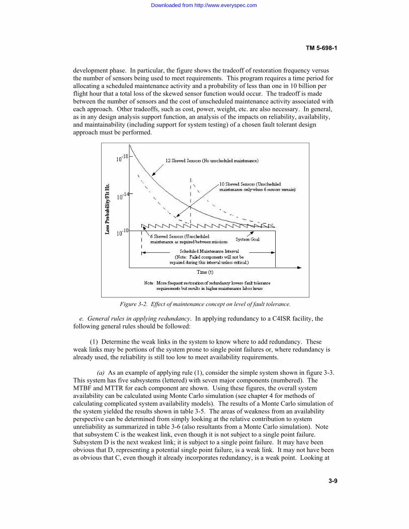
TM 5-698-1

3-9

development phase. In particular, the figure shows the tradeoff of restoration frequency versus the number of sensors being used to meet requirements. This program requires a time period for allocating a scheduled maintenance activity and a probability of less than one in 10 billion per flight hour that a total loss of the skewed sensor function would occur. The tradeoff is made between the number of sensors and the cost of unscheduled maintenance activity associated with each approach. Other tradeoffs, such as cost, power, weight, etc. are also necessary. In general, as in any design analysis support function, an analysis of the impacts on reliability, availability, and maintainability (including support for system testing) of a chosen fault tolerant design approach must be performed.

Figure 3-2. Effect of maintenance concept on level of fault tolerance. e. General rules in applying redundancy. In applying redundancy to a C4ISR facility, the following general rules should be followed: (1) Determine the weak links in the system to know where to add redundancy. These weak links may be portions of the system prone to single point failures or, where redundancy is already used, the reliability is still too low to meet availability requirements. (a) As an example of applying rule (1), consider the simple system shown in figure 3-3. This system has five subsystems (lettered) with seven major components (numbered). The MTBF and MTTR for each component are shown. Using these figures, the overall system availability can be calculated using Monte Carlo simulation (see chapter 4 for methods of calculating complicated system availability models). The results of a Monte Carlo simulation of the system yielded the results shown in table 3-5. The areas of weakness from an availability perspective can be determined from simply looking at the relative contribution to system unreliability as summarized in table 3-6 (also resultants from a Monte Carlo simulation). Note that subsystem C is the weakest link, even though it is not subject to a single point failure. Subsystem D is the next weakest link; it is subject to a single point failure. It may have been obvious that D, representing a potential single point failure, is a weak link. It may not have been as obvious that C, even though it already incorporates redundancy, is a weak point. Looking at


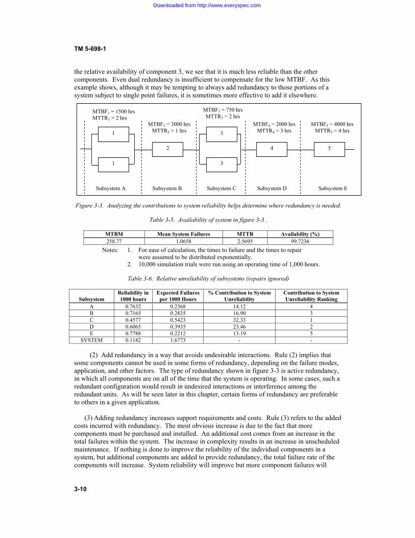
TM 5-698-1

3-10

the relative availability of component 3, we see that it is much less reliable than the other components. Even dual redundancy is insufficient to compensate for the low MTBF. As this example shows, although it may be tempting to always add redundancy to those portions of a system subject to single point failures, it is sometimes more effective to add it elsewhere.

Figure 3-3. Analyzing the contributions to system reliability helps determine where redundancy is needed.

Table 3-5. Availability of system in figure 3-3 .

MTBM Mean System Failures MTTR Availability (%) 258.77 1.0658 2.5695 99.7236

Notes: 1. For ease of calculation, the times to failure and the times to repair were assumed to be distributed exponentially.

2. 10,000 simulation trials were run using an operating time of 1,000 hours.

Table 3-6. Relative unreliability of subsystems (repairs ignored)

Subsystem

Reliability in 1000 hours

Expected Failures per 1000 Hours

% Contribution to System Unreliability

Contribution to System Unreliability Ranking

A 0.7632 0.2368 14.12 4 B 0.7165 0.2835 16.90 3 C 0.4577 0.5423 32.33 1 D 0.6065 0.3935 23.46 2 E 0.7788 0.2212 13.19 5

SYSTEM 0.1182 1.6773 - - (2) Add redundancy in a way that avoids undesirable interactions. Rule (2) implies that some components cannot be used in some forms of redundancy, depending on the failure modes, application, and other factors. The type of redundancy shown in figure 3-3 is active redundancy, in which all components are on all of the time that the system is operating. In some cases, such a redundant configuration would result in undesired interactions or interference among the redundant units. As will be seen later in this chapter, certain forms of redundancy are preferable to others in a given application. (3) Adding redundancy increases support requirements and costs. Rule (3) refers to the added costs incurred with redundancy. The most obvious increase is due to the fact that more components must be purchased and installed. An additional cost comes from an increase in the total failures within the system. The increase in complexity results in an increase in unscheduled maintenance. If nothing is done to improve the reliability of the individual components in a system, but additional components are added to provide redundancy, the total failure rate of the components will increase. System reliability will improve but more component failures will

2 4 5

1

1

3

3

MTBF1 = 1500 hrs MTTR1 = 2 hrs





Subsystem A Subsystem B Subsystem C Subsystem D Subsystem E


TM 5-698-1

3-11

occur. These failures will increase support requirements and costs. Redundancy also increases weight, space requirements, complexity, and time to design. Thus, safety and mission reliability are gained at the expense of adding an item(s) in the unscheduled maintenance chain. (a) The decision to use redundant design techniques must be based on analysis of the tradeoffs involved. Redundancy may prove to be the only available method, when other techniques of improving reliability (e.g., derating, simplification, better components) have been exhausted, or when methods of item improvement are shown to be more costly than duplications. (b) When preventive maintenance is planned, the use of redundant equipment can allow for repair with no system downtime. Occasionally, situations exist in which equipment cannot be maintained. In these cases, redundant elements may be the best way to significantly prolong operating time. (4) Ensure that any one redundant unit can be maintained without shutting down the other redundant units. Rule (4) requires that we ensure that any one redundant unit can be maintained without shutting down the other redundant units. Assume that two generators, for example, are sharing a load. If one fails and the operators must shut the other generator down to either gain access to or repair the failed generator, then there is no effective redundancy. An implicit assumption in using redundancy is that availability increases because we can repair a failed component while the remaining redundant components continue to operate. If this assumption is violated, redundancy will not increase availability. f. Design considerations. The FMEA is a primary reliability analysis, critical to the fault tolerant design process. The reliability engineer will use additional techniques as well for analyzing a fault tolerant design to verify that it meets reliability requirements. However, many of the evaluation tools used in the past are no longer adequate to deal with more sophisticated fault tolerant designs that include more complex fault handling capabilities. Because fault handling methods include the use of fault detection and fault recovery approaches, any evaluation tool must include the ability to properly account for the effects of imperfect fault detection and fault recovery. (1) Monte Carlo simulation and Markov techniques continue to be used as the primary means of analyzing highly sophisticated fault tolerant designs. These approaches have been modified to incorporate situations where the sequence of failure is important, where the failure is transient or intermittent, or where the response to failure (i.e., detection, isolation, recovery, and reconfiguration) is imperfect. In these situations, Markov methods continue to lead the way in evaluation methods. In general, the Markov approach, which is used to define the specific states that a system can occupy, has been used to incorporate fault handling and recovery. A major limitation to the Markov approach is that the number of system states that must be defined to comprehensively describe a large system and model the behavior of complex fault management schemes can become very large (approaching 105 for highly complex systems). A common solution to this problem is to partition the system into smaller systems, evaluate each partition separately, and then combine the results at the system level. However, such an approach is only exact when each partitioned subsystem's fault tolerant behavior is mutually independent of each other. If subsystem dependencies do exist, then an assumption of independence will result in only an approximate solution. (2) Other approaches that are now becoming more common involve decomposing the system into separate fault-occurrence and fault handling submodels. However, the inputs for this type of approach require knowledge of the distribution and parameter values of: detection,


TM 5-698-1

3-12

isolation, recovery, rates, etc. The following is a list of assumptions, limitations and sources of error found in existing reliability models: (a) Solving a fault-handling model in isolation and then reflecting its results in an aggregate model is, itself, an approximation technique. The assumptions necessary to determine a solution typically result in a lower bound (conservative) approximation of the system reliability. (b) Separate fault-handling models have been assumed to be independent of system state. This requires that the same fault-handling model and choice of parameters be used irrespective of the system's level of degradation. This ignores the fact that for many systems the recovery process is faster if the number of active units is smaller or that the recovery process may be different, depending on the sequence of events in different subsystems. (c) The common technique of partitioning the system into independent functional subgroups for computational ease is a potential source of error. The magnitude and direction of the error is a function of how truly independent/dependent the subgroups are of each other. If subgroups are assumed independent when in fact they are not, the effect is an overstatement of system reliability/availability. If subgroups are assumed completely dependent when some degree of independence exists, the effect is an understatement of the system's RAM capabilities. (d) Some models assume a constant instantaneous fault-protection coverage factor in lieu of a separate fault handling model. These fail to recognize that during time spent in the intermediate fault-handling states to detect, isolate, and recover/reconfigure, a second item failure could result in system failure. Further, as with fault handling models, these times are generally not constant, but depend on the current state of the system. (e) Most models require the assumption that the system is perfect at the mission start. Therefore, they cannot evaluate the effects of latent defects (e.g., handling, manufacturing, transportation, and prior mission), nor assist in determining the testability payoff or requirements for detection and removing them before the start of the mission. Models with this limitation cannot be used to evaluate alternate maintenance concepts that include degradation between missions as an acceptable strategy. (f) Some models require that spares be treated exactly like active units, irrespective of their actual utilization in the system mechanization. This requires that spares are assumed to be "hot" and have the same failure rates and failure modes as the active units. This assumption will cause the model to understate the system reliability in those situations where spares are "cold" or in "stand-by" and/or where their failure rates may be less that those of the active units. (g) As indicated previously, some models require the assumption that item failure rates are constant throughout time. This will result in an overstatement of system reliability if the items have failure rates that increase with mission time. Some models remove this restriction and permit time-varying failure rates. However, the solution algorithms employed require the use of global time (as opposed to local time of entry into a state), thus precluding the use of the model for repairable systems and availability analysis. 3-5. Improving availability through reliability-centered maintenance (RCM) All C4ISR facilities that are currently in operation require maintenance to continue to properly perform their functions and support their assigned missions. An effective and efficient maintenance program saves resources and maximizes availability. Reliability-Centered


TM 5-698-1

3-13

Maintenance (RCM) is an approach for developing an effective and efficient maintenance program based on the reliability characteristics of the constituent parts and subsystems, economics, and safety. a. RCM introduction. Prior to the development of the RCM methodology, it was widely believed that everything had a "right" time for some form of preventive maintenance (PM), usually replacement or overhaul. Despite this commonly accepted view, the results indicated that in far too many instances, PM seemed to have no beneficial effects, and, in many cases, actually made things worse by providing more opportunity for maintenance-induced failures. b. RCM definitions. The following definitions are commonly used in connection with RCM. (1) RCM is a logical, structured framework for determining the optimum mix of applicable and effective maintenance activities needed to sustain the operational reliability of systems and equipment while ensuring their safe and economical operation and support. (2) Maintenance is defined as those activities and actions that directly retain the proper operation of an item or restore that operation when it is interrupted by failure or some other anomaly. (Within the context of RCM, proper operation of an item means that the item can perform its intended function). (3) Corrective maintenance (CM) is maintenance required to restore a failed item to proper operation. Restoration is accomplished by removing the failed item and replacing it with a new item, or by fixing the item by removing and replacing internal components or by some other repair action. (4) Scheduled and condition-based preventive maintenance conducted to ensure safety, reduce the likelihood of operational failures, and obtain as much useful life as possible from an item. (5) Preventative maintenance is the act of doing maintenance in anticipation of some failure. Recent data collection efforts have indicated that PM programs are ineffective on a number of typical system components. An effective PM program will not only identify components that have predictable failures, but identify those that are random to avoid waste of maintenance resources. c. RCM overview. The RCM approach provides a logical way of determining if PM makes sense for a given item and, if so, selecting the appropriate type of PM. The approach is based on a number of factors. (1) RCM seeks to preserve system or equipment function. (2) RCM is more concerned on maintaining end system function than individual component function. (3) Use reliability as the basis for decisions. The failure characteristics of the item in question must be understood to determine the efficacy of preventive maintenance. (4) Consider safety first and then economics. Safety must always be preserved. When safety is not an issue, preventive maintenance must be justified on economic grounds.


TM 5-698-1

3-14

(5) Acknowledge design limitations. Maintenance cannot improve the inherent reliability; it is dictated by design (6) Treat RCM as a continuing process. The difference between the perceived and actual design life and failure characteristics is addressed through age (or life) exploration. d. Preventive maintenance. RCM has changed the approach to preventive maintenance. The RCM concept has completely changed the way in which PM is viewed. It is now widely accepted that not all items benefit from PM, and it is often less expensive to allow an item to run to failure rather than to do PM. e. Condition monitoring and analysis. Some impending failures can be detected using some form of condition monitoring and analysis, a type of preventive maintenance. Condition monitoring is defined as periodically or continuously checking physical characteristics or operating parameters of an item. Based on analyzing the results of condition monitoring, a decision is made to either take no action or to replace or repair the item. Condition monitoring can be performed through inspection, or by monitoring performance or other parameters. f. The RCM concept. RCM has two primary objectives: to ensure safety through preventive maintenance actions, and, when safety is not a concern, preserve functionality in the most economical manner. Preventive maintenance is applicable only if it is both effective and economically viable. When safety is not a consideration and PM is either not effective or less economical than running to failure, only CM is required. (1) PM can be effective only when there is a quantitative indication of an impending functional failure or indication of a hidden failure. That is, if reduced resistance to failure can be detected (potential failure) and there is a consistent or predictable interval between potential failure and functional failure, then PM is applicable. (2) The costs incurred with any PM being considered for an item must be less than for running the item to failure (economic viability). The failure may have operational or non-operational consequences. The two categories of cost included in such a comparison for these two failure consequences are operational - the indirect economic loss as a result of failure and the direct cost of repair, and non-operational - the direct cost of repair. g. A product can fail in two basic ways. First, it can fail to perform one or more of the functions for which it was designed. Such a failure is called a functional failure. Second, a product can fail in such a way that no function is impaired. The failure could be something as simple as a scratch or other damage of the finish of the product. Or it could be that one of two redundant items, only one of which is required for a given function, has failed. h. The three categories of failure consequences generally used in RCM analysis are Safety, Operational, and Economic. If a functional failure directly has an adverse affect on operating safety, the failure effect is categorized as Safety. When the failure does not adversely affect safety but prevents the end system from completing a mission, the failure is categorized as an Operational failure. When a functional failure does not adversely affect safety and does not adversely affect operational requirements, then the failure is said to have an Economic effect. The only penalty of such a failure is the cost to repair the failure.


TM 5-698-1

3-15

3-6. Application of RCM to C4ISR facilities For equipment used in facilities, condition monitoring, including inspections, overhauls, lubrication, servicing, and failure-finding tasks are all routinely part of an RCM-based preventive maintenance program. C4ISR facilities potentially require all these tasks. More detailed information on applying RCM to C4ISR facilities appears in TM 5-698-2.


TM 5-698-1

4-1

CHAPTER 4

ASSESSING RELIABILITY AND AVAILABILITY OF C4ISR FACILITIES

4-1. Purpose of the assessment As systems become more and more complex, good methods for specifying and analyzing the systems and their sub-systems become more important. Reliability modeling (including prediction, evaluation, and control) is vital for proper design, dependable operation, and effective maintenance of systems. The popularity of designing redundancy into systems poses additional challenges to reliability professionals. For the various kinds of redundant systems, the reliability and availability are extremely sensitive to even small variations in certain parameters; thus, precise understanding and insight can be gained only by modeling. The purpose of this chapter is to provide the reader with an understanding of reliability modeling to assist in the decision making process for facility improvement. The need to assess the reliability, availability, and maintainability of a system is becoming more important as organizations understand the potential effects of failures and downtime for the systems. Regardless of what mission is being served, or who the intended customer may be, it should be a reasonable assumption to state that the degree of product/service success is directly related to the ability of that product/service to meet or exceed customer expectations. The eight-step process shown in table 4-1 should be adhered to during a reliability study. Validation is essential throughout the eight-step process.

Table 4-1. Steps in performing a reliability analysis.

1) Problem Definition: define problem and its objectives. 2) Model Building: description of system's entities and their interaction. 3) Data Collection: quantify probability distributions for system's entities. 4) Program: select programming language or software package to execute. 5) Verification: check that code is achieving expected results. 6) Experimental Design: determine initial conditions, simulation period and number of runs (must be statistically valid). 7) Implementation: run model and test its sensitivity to variations. 8) Documentation: document reliability study to verify problem definition objectives are reached (document enough for functional model in future).

4-2. Prediction There are many valid reasons for predicting reliability. One purpose for reliability prediction is to assess the reliability of a proposed design and to provide a quantitative basis for selection among competing approaches or components. In addition, prediction results can be used to rank design problem areas and assess trade study results. A combination of prediction methods should be used to assess progress in meeting design goals, identifying environmental concerns, controlling critical items and determining end-of-life failure mechanisms. Making predictions should be an ongoing activity that starts with the initial design concept and continues through the evaluation of alternate design approaches, redesigns, and corrective actions. Each iteration of prediction should


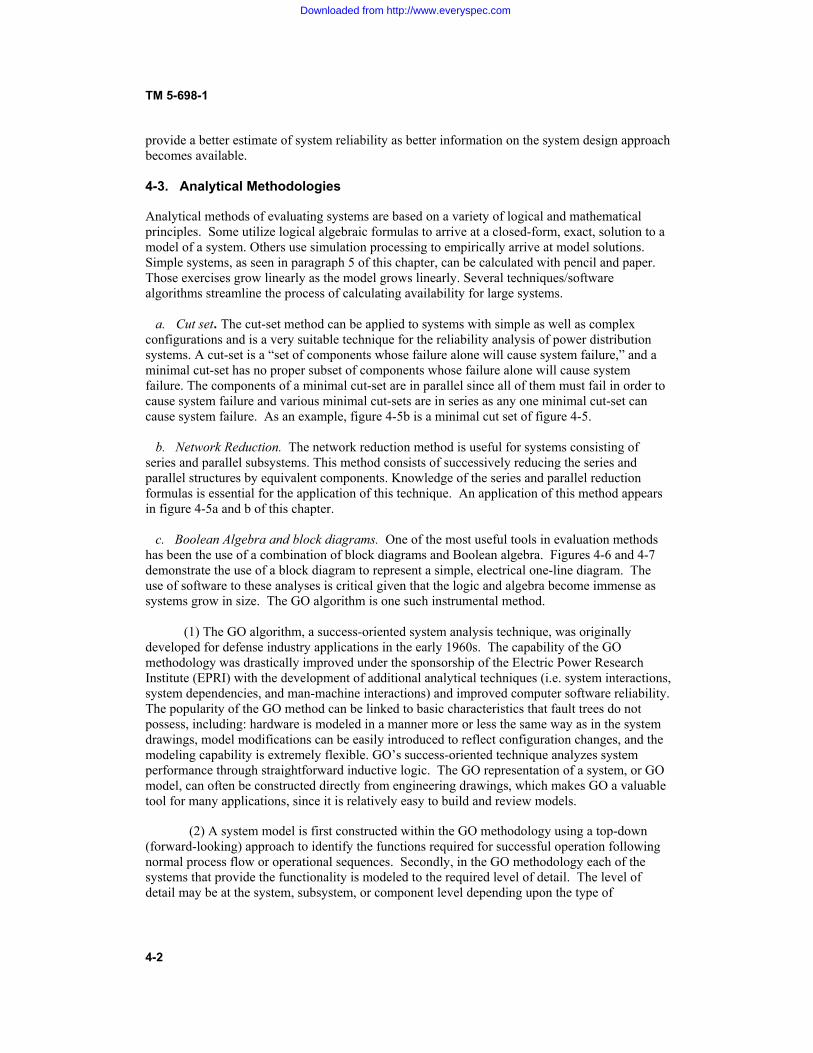
TM 5-698-1

4-2

provide a better estimate of system reliability as better information on the system design approach becomes available. 4-3. Analytical Methodologies

Analytical methods of evaluating systems are based on a variety of logical and mathematical principles. Some utilize logical algebraic formulas to arrive at a closed-form, exact, solution to a model of a system. Others use simulation processing to empirically arrive at model solutions. Simple systems, as seen in paragraph 5 of this chapter, can be calculated with pencil and paper. Those exercises grow linearly as the model grows linearly. Several techniques/software algorithms streamline the process of calculating availability for large systems. a. Cut set. The cut-set method can be applied to systems with simple as well as complex configurations and is a very suitable technique for the reliability analysis of power distribution systems. A cut-set is a “set of components whose failure alone will cause system failure,” and a minimal cut-set has no proper subset of components whose failure alone will cause system failure. The components of a minimal cut-set are in parallel since all of them must fail in order to cause system failure and various minimal cut-sets are in series as any one minimal cut-set can cause system failure. As an example, figure 4-5b is a minimal cut set of figure 4-5. b. Network Reduction. The network reduction method is useful for systems consisting of series and parallel subsystems. This method consists of successively reducing the series and parallel structures by equivalent components. Knowledge of the series and parallel reduction formulas is essential for the application of this technique. An application of this method appears in figure 4-5a and b of this chapter. c. Boolean Algebra and block diagrams. One of the most useful tools in evaluation methods has been the use of a combination of block diagrams and Boolean algebra. Figures 4-6 and 4-7 demonstrate the use of a block diagram to represent a simple, electrical one-line diagram. The use of software to these analyses is critical given that the logic and algebra become immense as systems grow in size. The GO algorithm is one such instrumental method. (1) The GO algorithm, a success-oriented system analysis technique, was originally developed for defense industry applications in the early 1960s. The capability of the GO methodology was drastically improved under the sponsorship of the Electric Power Research Institute (EPRI) with the development of additional analytical techniques (i.e. system interactions, system dependencies, and man-machine interactions) and improved computer software reliability. The popularity of the GO method can be linked to basic characteristics that fault trees do not possess, including: hardware is modeled in a manner more or less the same way as in the system drawings, model modifications can be easily introduced to reflect configuration changes, and the modeling capability is extremely flexible. GO’s success-oriented technique analyzes system performance through straightforward inductive logic. The GO representation of a system, or GO model, can often be constructed directly from engineering drawings, which makes GO a valuable tool for many applications, since it is relatively easy to build and review models.

(2) A system model is first constructed within the GO methodology using a top-down (forward-looking) approach to identify the functions required for successful operation following normal process flow or operational sequences. Secondly, in the GO methodology each of the systems that provide the functionality is modeled to the required level of detail. The level of detail may be at the system, subsystem, or component level depending upon the type of


TM 5-698-1

4-3

information required and the plant specific information available. The GO models determine all system-response modes: successes, failures, prematures, etc.

(3) GO models consist of arrangements of GO operator symbols and represent the engineering functions of components, subsystems, and systems. The models are generally constructed from engineering (one-line) drawings by replacing engineering elements (valves, motors, switches, etc.) with one or more GO symbols that are interrelated to represent system functions, logic, and operational sequences. The GO software uses the GO model to quantify system performance. The method evaluates system reliability and availability, identifies fault sets, ranks the relative importance of the constituent elements, and places confidence bounds on the probabilities of occurrence of system events reflecting the effects of data uncertainties.

Some key features of the GO method are: • Models follow the normal process flow • Most model elements have one-to-one correspondence with system elements • Models accommodate component and system interactions and dependencies • Models are compact and easy to validate • Outputs represent all system success and failure states • Models can be easily altered and updated • Fault sets can be generated without altering the basic model • System operational aspects can be incorporated • Numerical errors due to pruning are known and can be controlled

(4) The GO procedure uses a set of seventeen standard logical operators to represent the logic operation, interaction, and combination of physical equipment and human actions. For example, a type 1 operator represents the logical operation of equipment which either performs, or fails to perform, its function given a proper input or stimulus. The type 2 operator performs the logical OR gate operation where a successful response is generated if any of several inputs is proper, etc. The Random variables of the GO methodology include operator inputs called stimuli (S1, S2,…Sn) and outputs referred to as responses (R1, R2,…, Rn). An operator, which represents equipment responses or human actions, and which may itself have associated performance probabilities, process the input random variable in a prescribed and well-defined way to generate the output random variables. These random variables are given the electrical term “signals” in the GO models d. State Space. The State Space methodology is founded on a more general mathematical concept called Markov Chains. Markov Chains employ a modeling technique that describes a system by the possible states in which it can possess (i.e. State Space). For our purpose, a system essentially resides in two distinct states: up or down. The probability of transitioning from one state to the other in a given time period is the critical reliability metric we are after. Figure 4-1 shows this simple Markov model.


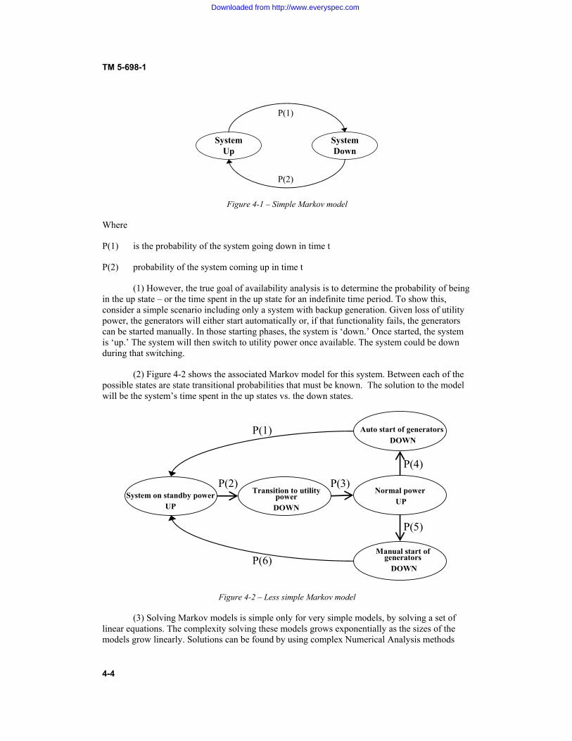
TM 5-698-1

4-4

System Up

P(1)

P(2)

System Down

Figure 4-1 – Simple Markov model

Where

P(1) is the probability of the system going down in time t

P(2) probability of the system coming up in time t

(1) However, the true goal of availability analysis is to determine the probability of being in the up state – or the time spent in the up state for an indefinite time period. To show this, consider a simple scenario including only a system with backup generation. Given loss of utility power, the generators will either start automatically or, if that functionality fails, the generators can be started manually. In those starting phases, the system is ‘down.’ Once started, the system is ‘up.’ The system will then switch to utility power once available. The system could be down during that switching.

(2) Figure 4-2 shows the associated Markov model for this system. Between each of the possible states are state transitional probabilities that must be known. The solution to the model will be the system’s time spent in the up states vs. the down states.

Normal powerUP

Auto start of generators DOWN

Manual start of generators

DOWN

System on standby power UP

Transition to utility power

DOWN

P(1)

P(6)

P(5)

P(4)

P(2) P(3)

Figure 4-2 – Less simple Markov model

(3) Solving Markov models is simple only for very simple models, by solving a set of linear equations. The complexity solving these models grows exponentially as the sizes of the models grow linearly. Solutions can be found by using complex Numerical Analysis methods


TM 5-698-1

4-5

involving Linear Algebraic matrix operations, etc. Markov models can also be solved by Monte Carlo techniques described below. e. Monte Carlo Simulation. Monte Carlo Simulation is the most versatile modeling methodology available. The methodology can be implemented in many forms from simple models in a spreadsheet environment to complex models that are ‘hand crafted’ in a programming language of choice. There are also a variety of simulation software packages that provide drag-and-drop environments that can automate the creation of simulated models for the casual analyst. (1) The Monte Carlo Simulator operates on an iterative process where each ‘iteration’ represents a description of what the system could experience through a set mission life. For instance, if we consider the past experience of a system, including what really failed, that experience was only one of infinite possible outcomes that depended on the failure characteristics of that system.

(2) Thus, Monte Carlo Simulation looks forward by considering possible scenarios that could occur in the future – and those scenarios, with their associated likelihoods, are dependent on the failure characteristics applied to the system components. For each iteration, failure times and the associated repair attributes are picked for each component in the system. The simulation will then implement the logical relationships of the system to determine:

(a) If a failure has occurred in the system prior to the defined mission life.

(b) If a failed component(s) takes the system down, what is the duration of downtime? (3) With these items determined, the availability for the system in that particular iteration

can be calculated. Then, as this single iteration is repeated, an average is tabulated of uptime vs. downtime, and duration of downtimes. The average of all the iterations yields expected system availability.

(4) This method is extremely useful in calculating downtime based on different types of failure distributions. A component in a system may be repaired or replaced upon failure. Because many components that are replaced have failure distributions that are based on time in service, calculations must incorporate time-based failure distributions to accurately predict system availability. Simulation methods more readily accommodate this requirement.

(5) Figure 4-3 shows a sample timeline of the operation of two components. In this example, both components start in the available state. As the simulated time progresses, component failures are randomly generated based on that component’s operational RAM statistics. The figure shows the difference in series and redundant component orientation. In series, downtime occurs when either component fails; with redundancy, both components are required to fail to incur downtime.


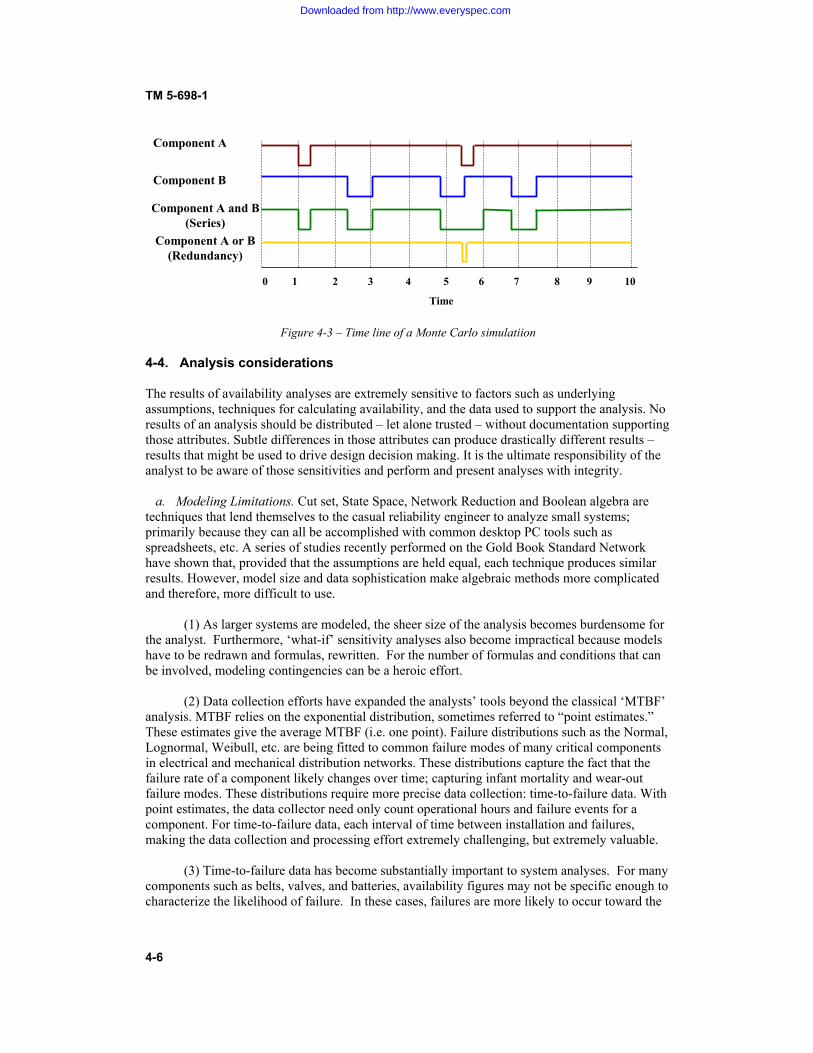
TM 5-698-1

4-6

Component A

Component B

0 1 2 3 4 5 6 7 8 9 10

Time

Component A and B(Series)

Component A or B(Redundancy)

Figure 4-3 – Time line of a Monte Carlo simulatiion 4-4. Analysis considerations The results of availability analyses are extremely sensitive to factors such as underlying assumptions, techniques for calculating availability, and the data used to support the analysis. No results of an analysis should be distributed – let alone trusted – without documentation supporting those attributes. Subtle differences in those attributes can produce drastically different results – results that might be used to drive design decision making. It is the ultimate responsibility of the analyst to be aware of those sensitivities and perform and present analyses with integrity. a. Modeling Limitations. Cut set, State Space, Network Reduction and Boolean algebra are techniques that lend themselves to the casual reliability engineer to analyze small systems; primarily because they can all be accomplished with common desktop PC tools such as spreadsheets, etc. A series of studies recently performed on the Gold Book Standard Network have shown that, provided that the assumptions are held equal, each technique produces similar results. However, model size and data sophistication make algebraic methods more complicated and therefore, more difficult to use. (1) As larger systems are modeled, the sheer size of the analysis becomes burdensome for the analyst. Furthermore, ‘what-if’ sensitivity analyses also become impractical because models have to be redrawn and formulas, rewritten. For the number of formulas and conditions that can be involved, modeling contingencies can be a heroic effort. (2) Data collection efforts have expanded the analysts’ tools beyond the classical ‘MTBF’ analysis. MTBF relies on the exponential distribution, sometimes referred to “point estimates.” These estimates give the average MTBF (i.e. one point). Failure distributions such as the Normal, Lognormal, Weibull, etc. are being fitted to common failure modes of many critical components in electrical and mechanical distribution networks. These distributions capture the fact that the failure rate of a component likely changes over time; capturing infant mortality and wear-out failure modes. These distributions require more precise data collection: time-to-failure data. With point estimates, the data collector need only count operational hours and failure events for a component. For time-to-failure data, each interval of time between installation and failures, making the data collection and processing effort extremely challenging, but extremely valuable. (3) Time-to-failure data has become substantially important to system analyses. For many components such as belts, valves, and batteries, availability figures may not be specific enough to characterize the likelihood of failure. In these cases, failures are more likely to occur toward the


TM 5-698-1

4-7

end of a component’s life – not evenly throughout its life. Simulation methods provide the means to include these considerations. b. Modeling Hurdles. There are several system attributes that are challenging to model. UPS battery life, for instance, had historically been assumed to be limitless in many analyses – whereas their contribution to power availability is not. Furthermore, data has shown that standby equipment has differing distributions from their primary counterparts. Thirdly, spare parts availability, human factors, etc. are difficult to capture with the classical approaches to availability analysis. c. Modeling Data. The underlying data that supports a reliability assessment can be as important as the model itself. Data must be scrutinized to ensure that the results are realistic and defendable. There are a variety of sources of component reliability data. Army technical manual Survey of Reliability and Availability Information for Power Distribution, Power Generation and Heating, Ventilating and Air Conditioning (HVAC) Components for Commercial, Industrial and Utility Installations (TM 5-698-5) contains data collected by the US Army Corps of Engineers. This dataset was collected and summarized for the distinct propose of modeling C4ISR facilities. d. Modeling Solutions. The typical engineer can perform ‘back of the envelope’ analyses easily. Results from these analyses are only as good as the assumed ground rules and the data used. Experience has shown that analysts who wish to perform availability studies often and consistently should choose a software package to aid in this effort. Packages exist that perform analyses via most of the described methodologies. Once a package is selected, the user should become familiar with the package behavior, the analytical or numerical methodology used, and the underlying limitations of that package. 4-5 Modeling Examples

No matter what methodology is chosen for a reliability analysis, the expected results, provided that the underlying assumptions are held fixed, should be consistent across all methods. The analyst should develop a sense of the expected results of small systems, and have a feel for the effects of increments changes to a system when made. Below are a series of small examples that will illustrate typical results in simple models. a. Modeling Basics. Reliability modeling generally begins with referring to a one-line drawing for the electrical, mechanical, and control systems. In addition to these resources, the analyst should have a firm understanding of the theory of operation of the system to be modeled. These sources of information will form the basis for the structure and behavior of the system that is to be modeled. (1) For this manual, we adopt a pseudo diagramming technique that can be applied to, or converted to, whichever modeling technique is chosen. The convention can be most accurately described as a Reliability Block Diagram (RBD). Figure 4-4 shows a typical one-line diagram representation of a generator/bus and its corresponding RBD representation.


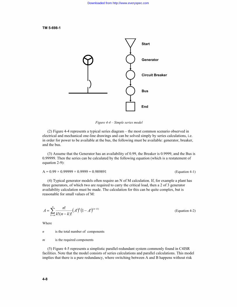
TM 5-698-1

4-8

Start

Generator

Circuit Breaker

Bus

End

Figure 4-4 – Simple series model (2) Figure 4-4 represents a typical series diagram – the most common scenario observed in electrical and mechanical one-line drawings and can be solved simply by series calculations, i.e. in order for power to be available at the bus, the following must be available: generator, breaker, and the bus. (3) Assume that the Generator has an availability of 0.99, the Breaker is 0.9999, and the Bus is 0.99999. Then the series can be calculated by the following equation (which is a restatement of equation 2-9): A = 0.99 × 0.99999 × 0.9999 = 0.989891 (Equation 4-1) (4) Typical generator models often require an N of M calculation. If, for example a plant has three generators, of which two are required to carry the critical load, then a 2 of 3 generator availability calculation must be made. The calculation for this can be quite complex, but is reasonable for small values of M:

� � � �¦

��

n

mk

knk AAknk

nA )('1')!(!

! (Equation 4-2)

Where

n is the total number of components

m is the required components (5) Figure 4-5 represents a simplistic parallel-redundant system commonly found in C4ISR facilities. Note that the model consists of series calculations and parallel calculations. This model implies that there is a pure redundancy, where switching between A and B happens without risk


TM 5-698-1

4-9

of failure. In most cases, there are reliability considerations in the switching between redundant systems.

Start

Circuit Breakers

Bus

OR

Redundant UPS

Circuit Breakers

End

A B

A B

Figure 4-5 – Simple parallel model (6) The model described by Figure 4-5 can also be solved with simple calculations. Assume that the Bus has an availability of 0.99999, the Breakers are 0.9999, and the UPS is 0.999. To determine the system availability, one must reduce the network to simpler series and parallel models. The general sequence is to reduce the Breaker-UPS-Breaker series to one value. Then calculate the redundant OR operator followed by treating that result as a value in series with the Bus. The Breaker-UPS-Breaker series can be computed by AUPS = 0.9999 × 0.999 × 0.9999 = 0.9988002 (Equation 4-3) Now, with that reduction, the model can be represented by Figure 4-5a.


TM 5-698-1

4-10

Start

Bus

OR

Breaker-UPS Series

End

A B

Figure 4-5a – Simple parallel model, first reduction Next we reduce the OR calculation to one availability value: AOR = 1-[(1-0.9988002) × (1-0.9988002)] = 0.99999856 (Equation 4-4) Figure 4-5b shows this further reduction.

Start

Bus

A or B UPS Series

End

Figure 4-5b – Simple parallel model, second reduction Then, this system, now reduced to a series system, can be easily calculated by AFinal = 0.99999 × 0.99999856 = 0.99998856 (Equation 4-5) (7) Building controls contingencies into reliability models is prudent. Often pure OR gates result in availability values that are inflated because they do not include the probability of the switching action itself. Whether the control is automatic via PLC or SCADA, or requires maintenance personnel to manually make the switch, the redundancy is limited by that switching action. (8) Consider Figure 4-6 where a facility utilizes dual chilled water pumps. If Pump A fails (or is taken down for maintenance) the valves supporting Pump A must be closed and the valves


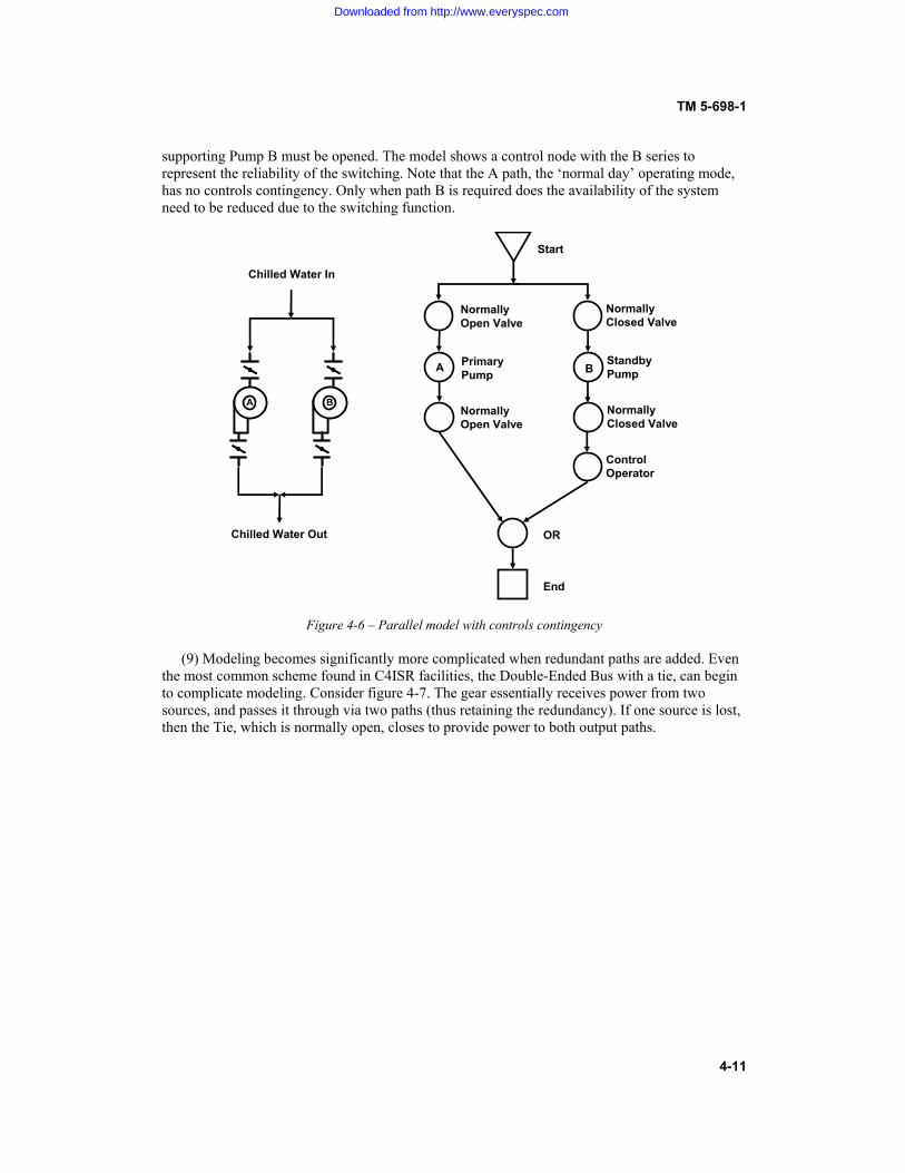
TM 5-698-1

4-11

supporting Pump B must be opened. The model shows a control node with the B series to represent the reliability of the switching. Note that the A path, the ‘normal day’ operating mode, has no controls contingency. Only when path B is required does the availability of the system need to be reduced due to the switching function.

Start

Normally Open Valve

OR

Primary Pump

Normally Open Valve

End

B

A B

Normally Closed Valve

Standby Pump

Normally Closed Valve

Control Operator

A

Chilled Water In

Chilled Water Out

Figure 4-6 – Parallel model with controls contingency

(9) Modeling becomes significantly more complicated when redundant paths are added. Even the most common scheme found in C4ISR facilities, the Double-Ended Bus with a tie, can begin to complicate modeling. Consider figure 4-7. The gear essentially receives power from two sources, and passes it through via two paths (thus retaining the redundancy). If one source is lost, then the Tie, which is normally open, closes to provide power to both output paths.


TM 5-698-1

4-12

Supply A Supply B

Tie Breaker

Output A Output B

Figure 4-7 – Double Ended Bus A typical model of this system is illustrated in Figure 4-8

Start

Input Circuit Breaker A

Start

Input Circuit Breaker B

Start

Bus A

Start

Bus B

Start

Tie Breaker

AND

OR

AND AND

AND

OR

Output Circuit Breaker A


Figure 4-8 – Model of a Double Ended Bus (10) The key to the logic lies in the fact that typical modeling can not readily emulate that power can pass through the tie in both directions. Thus, the availabilities of the tie and the busses are created independently, and used within the logic where required. (11) If one looks at the logic behind the availability of power out of a breaker on bus A, then the critical ‘OR’ statement is joining the following two scenarios:

(a) Power available from source A (b) Power required from source B

(12) In case (a), the only required components are the incoming breaker, (on side A) the Bus A, and the outgoing breaker A. Case (b) requires much more. In order of how the power will flow if source A is unavailable: Input Breaker B, Bus B, Tie, Bus A, output Breaker A. Figures 4-9 and 4-10 show these two cases, with the pivotal OR block shaded black.


TM 5-698-1

4-13

Start

Input Circuit Breaker A

Start

Bus A

AND

OR


Figure 4-9 – Model of a Double Ended Bus, Case 1

Start

Input Circuit Breaker B

Start

Bus A

Start

Bus B

Start

Tie Breaker

AND

AND


OR

Figure 4-10 – Model of a Double Ended Bus, Case 2 4-6 Modeling Complexities The modeling examples discussed previously represent a top-down style of modeling, and is the most common type of modeling. The model has a beginning and an end. Failures within the model interrupt the availability of downstream components. This style has a variety of advantages, one being that it loosely follows the intuitive paths of, say, power or chilled water. There are some disadvantages and limitations to top down modeling: upstream effects of failures, loop systems, and UPS systems. In most cases, advanced simulation methods need to be employed to capture these complexities. a. Effects of unique failure modes. The failure of a component in a system typically has an effect on the remainder of the system downstream of the failure only. Unfortunately, there are some failures, or particular failure modes of a component, that can have effects on the system upstream. For example, if a circuit breaker fails to open on command, i.e. there is a downstream fault that the breaker is intended to protect against, but doesn’t. That fault can be passed upstream and have an effect on a much larger portion of the entire system then just those components


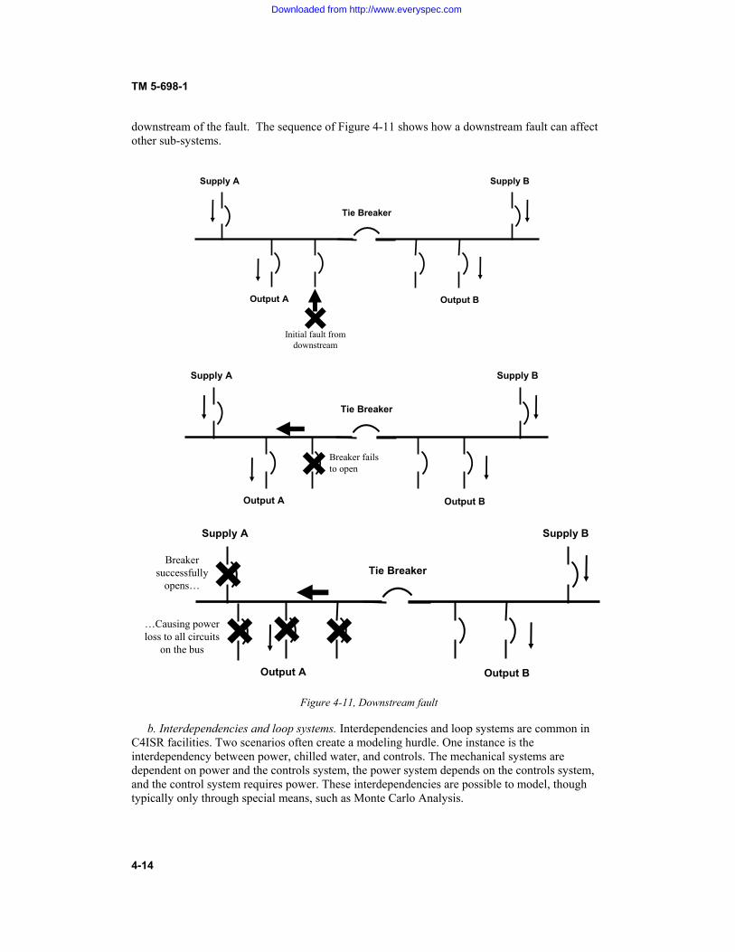
TM 5-698-1

4-14

downstream of the fault. The sequence of Figure 4-11 shows how a downstream fault can affect other sub-systems.

Supply A Supply B

Tie Breaker

Output A Output B×Initial fault from downstream

Supply A Supply B

Tie Breaker

Output A Output B

×Breaker fails to open

Supply A Supply B

Tie Breaker

Output A Output B

××× ×

Breaker successfully

opens…

…Causing power loss to all circuits

on the bus

Figure 4-11, Downstream fault b. Interdependencies and loop systems. Interdependencies and loop systems are common in C4ISR facilities. Two scenarios often create a modeling hurdle. One instance is the interdependency between power, chilled water, and controls. The mechanical systems are dependent on power and the controls system, the power system depends on the controls system, and the control system requires power. These interdependencies are possible to model, though typically only through special means, such as Monte Carlo Analysis.


TM 5-698-1

4-15

c. UPS systems. Uninterruptible power supply systems present a unique challenge to the analyst because capturing the effects on availability from the added battery backup can be difficult. The concept of operation for a UPS is limited to the fact that the battery has a limited life. If, for instance, a UPS has 45 minutes of ride-through time, then any upstream interruption less then 45 minutes will essentially be mitigated. However, if an interruption lasts longer then 45 minutes, the total interruption time is essentially shortened by 45 minutes before the downstream mission is lost. Below are two simple cases to illustrate this point.

Assume that over the course of one year, a system experiences a failure upstream of the UPS: Case 1: the failing component is repaired within 30 minutes. In this case the UPS provides sufficient downstream power and the mission remains available. This case yields an availability of 8766/8766 = 1. Availability is retained. Case 2: the failing component requires 24 hours to repair. In this case the UPS merely reduces the downtime of the mission to 24 hrs – 45 minutes, or 23.25 hrs. In this case the availability for the case-year is (8766-23.25)/8766 or 0.9973.

d. Conclusion of Complexities. Complex modeling scenarios need complex modeling techniques. In most cases Monte Carlo methods need to be employed. Monte Carlo methods capture true operating scenarios, one iteration at a time, as set up by the analyst. Simulation allows the analyst to interject nearly any conceivable operating anomaly that might occur in a facility. 4-7 Conclusion RAM studies should be conducted with the intent of capturing the actual behavior of the facility. This goal will force the analyst to continually seek better data and better modeling techniques. Although, in design, RAM can not be perfectly captured; it is still just a prediction. Refined assessment techniques can uncover previously unforeseen contingencies that may cause a mission to be lost. a. RAM analysis. RAM analysis must be continuously improved to converge with the behavior of a system. As systems become more complex, the methods will undoubtedly become more complex as well. The analyst should always compare his modeling assumptions and attributes captured to the actual operation of the system being modeled. New techniques must continuously be explored to see that the gap between the models and the true system narrows. b. Verification. Facility managers must verify that the model is valid – capturing his or her system accurately. He or she must also be aware of the reliability data that supports the model. The model is only as good as the data that it uses. In a sense, the data is a single-point-vulnerability for the accuracy of the model. Facility managers and reliability analysts alike should always consult the most recent TM for reliability data. Further, adoption of a continuous RAM process such as reliability centered maintenance will provide actual system behavior data that will continue to serve the reliability, availability, and maintainability goals over the life of the system.


TM 5-698-1

A-1

APPENDIX A

REFERENCES

REQUIRED PUBLICATIONS Government Publications Department of the Army

TM 5-698-2 Reliability Centered Maintenance for C4ISR Facilities (RCM) (Cited in paragraphs 1-3 and 3-6). TM 5-698-3 Reliability Primer for C4ISR Facilities (Cited in paragraph 1-3). TM 5-698-4 Failure Modes and Effects Analysis for C4ISR Facilities (FMECA,) (Cited in paragraph 1-3) TM 5-698-5 Survey of Reliability and Availability Information for Power Distribution, Power Generation and Heating, Ventilating and Air Conditioning (HVAC) Components for Commercial, Industrial and Utility Installations (Cited in paragraphs 1-3 and 4-4c). TM 5-698-6 Reliability Data Collection Manual (Cited in paragraph 1-3).

RELATED PUBLICATIONS Government Publications

MIL-HDBK-189 Reliability Growth Management MIL-HDBK-781 Reliability Test Methods, Plans and Environments for Engineering Development, Qualification & Production

Non-Government Publications Abernethy, Dr. R.B., “The New Weibull Handbook,” Gulf Publishing Co., Houston, TX, 1994.

AIAG MFMEA-1 (Automotive Industry Action Group, Machinery Failure Mode & Effects Analysis), www.aiag.com, Potential Failure Mode & Effects Analysis for Tooling & Equipment.

Blanchard, Benjamin S. and Wolter J. Fabrycky, Systems Engineering and Analysis, Prentice-Hall, Inc., January 1998.


TM 5-698-1

A-2

Burkhard, Alan H., “Deterministic Failure Prediction,” 1987 Proceedings Annual Reliability and Maintainability Symposium, IEEE, 1987. Carter, A.D.S., Mechanical Reliability , John Wiley & Sons, 1986. IEC Electronics Corporation, www.iec-electronics.com, IEC 60300-1, Dependability Programme Management - Part 1: Dependability Programme Management. IEC 60300-2, Dependability Management - Part 2: Dependability Programme Elements and Tasks and IEC 60300, Part 3-11, “Dependability Management – Part 3: Application Guide – Section 11: Reliability Centered Maintenance. Institute of Electrical and Electronics Engineers 445 Hoes Lane, P.O. Box 1331, Piscataway, NJ 08855-1331, www.ieee.org

ANSI/IEEE 762 - Standard Definitions for Use in Reporting Electric Generating Unit Reliability, Availability, and Productivity. Coyle, Timothy, Arno, Robert G., and Hale, Peyton S., “GO Reliability Methodology Applied to Gold Book Standard Network,” IEEE Transactions on Reliability, IEEE, 2002. “Operational Maintenance Data for Power Generation Distribution and HVAC Components,” IEEE Transactions on Industry Applications, March/April 1999.

“Survey of Reliability and Availability Information for Power Distribution, Power Generation, and HVAC Components for Commercial, Industrial, and Utility Installations,” IEEE Transactions on Industry Applications, January/February 2001.

Heidtmann, Klaus D., “Deterministic Reliability-Modeling of Dynamic Redundancy,” IEEE Transactions on Reliability, Volume 41, Number 3, IEEE, September 1992.

Ireson, W.G., Handbook of Reliability Engineering and Management, McGraw-Hill, 1988.

Kapur, K.C. and L.R. Lamberson, Reliability in Engineering Design, John Wiley & Sons, 1977.

Kececioglu, D, Reliability Engineering Handbook, 2 Vols., Prentice-Hall, 1991.

Moubray, John, Reliability-Centered Maintenance II, Industrial Press, New York, NY, April 1997. NASA, National Aeronautics and Space Administration, www.nasa.gov

National Aeronautics and Space Administration, “Reliability Centered Maintenance Guide for Facilities and Collateral Equipment,” December 1996.

Nelson, Dr. Wayne, Accelerated Testing; Statistical Models, Test Plans and Data Analysis, John Wiley & Sons, 1990.


TM 5-698-1

A-3

Nowlan, F.S. and H.F. Heap, “Reliability-Centered Maintenance,” DoD, 1978, available from Maintenance Quality Systems, LLC, 1127-F Benfield Blvd, Suite F, Millersville, MD 21108-2540, www.mqsllc.com. O’Connor, P.D.T., Practical Reliability Engineering, John Wiley & Sons. Pecht, Michael, Product Reliability, Maintainability, and Supportability Handbook, ARINC Research Corporation, CRC Press, www.crcpress.com, 1995. Reliability Analysis Center, 201 Mill Street Rome, NY 13440, www.rac.iitri.org.

Reliability Analysis Center, Fault Tree Application Guide, 1990. Reliability Analysis Center, Failure Modes Effects and Criticality Analysis, 1993. Reliability Analysis Center, Reliability Toolkit: Commercial Practices Editions, 1994

Smith, Anthony M., Reliability-Centered Maintenance, McGraw Hill, New York, NY, September1992 Society of Automotive Engineers, 755 W. Big Beaver, Suite 1600, Troy, MI 48084, www.sae.org.

SAE JA1000: Reliability Program Standard. SAE JA1000/1: Reliability Program Standard Implementation Guide.

Society of Automotive Engineers, “Evaluation Criteria for Reliability-Centered Maintenance (RCM) Processes,” JA1011, August 1999. Society of Automotive Engineers, “A Guide to the Reliability-Centered Maintenance (RCM) Standard,” JA1012, Draft, June 2000.

Talmor, Michael, and Arueti, Shimshon, “Reliability Prediction: The Turnover Point,” 1997 Proceedings Annual Reliability and Maintainability Symposium, IEEE, 1997. Wang, Wendai, and Kececioglu, Dimitri B., “Confidence Limits on the Inherent Availability of Equipment,” 2000 Proceedings Annual reliability and Maintainability Symposium, IEEE, 2000.

. Wadsworth, H.M., Handbook of Statistical Methods for Engineers and Scientists, McGraw Hill, 1989.


TM 5-698-1

B-1

APPENDIX B

THE MATHEMATICS OF RELIABILITY

B-1. Introduction to the mathematics of reliability This appendix provides the reader with an overview of the mathematics of reliability theory. It is not pre-sented as a complete (or mathematically rigorous) discussion of probability theory but should give the reader a reasonable understanding of how reliability is calculated. Before beginning the discussion, a key point must be made. Reliability is a design characteristic indicating a product's ability to perform its mis-sion over time without failure or to operate without logistics support. In the first case, a failure can be defined as any incident that prevents the mission from being accomplished; in the second case, a failure is any incident requiring unscheduled maintenance. Reliability is achieved through sound design, the proper application of parts, and an understanding of failure mechanisms. It is not achieved by estimating it or calculating it. Estimation and calculation are, however, necessary to help determine feasibility, assess progress, and provide failure probabilities and frequencies to spares calculations and other analyses. With that in mind, let's first look at the theory of probability. B-2. Uncertainty - at the heart of probability The mathematics of reliability is based on probability theory. Probability theory, in turn, deals with un-certainty. Probability had its origins in gambling. Some gamblers, hoping to improve their luck, turned to mathematicians with questions like what are the odds against rolling a six on a die, of drawing a deuce from a deck of 52 cards, or of having a tossed coin come up heads. In each case, probability can be thought of as the relative frequency with which an event will occur in the long run. When we assert that tossing an honest coin will result in heads (or tails) 50% of the time, we do not mean that we will neces-sarily toss five heads in 10 trials. We only mean that in the long run, we would expect to see 50% heads and 50% tails. Another way to look at this example is to imagine a very large number of coins being tossed simultaneously; again, we would expect 50% heads and 50% tails. a. Events. Why is there a 50% chance of tossing a head on a given toss of a coin? It is because there are two results, or events, that can occur (assume that it is very unlikely for the coin to land on its edge) and for a balanced, honest coin, there is no reason for either event to be favored. Thus, we say the out-come is random and each event is equally likely to occur. Hence, the probability of tossing a head (or tail) is the probability one of two equally probable events occurring = 1/2 = 0.5. Now consider a die. One of six equally probable events can result from rolling a die: we can roll a one, two, three, four, five, or six. The result of any roll of a die (or of a toss of a coin) is called a discrete random variable. The probability that on any roll this random variable will assume a certain value, call it x, can be written as a function, f(x). We refer to the probabilities f(x), specified for all values of x, as values of the probability function of x. For the die and coin, the function is constant. For the coin, the function is f(x) = 0.5, where x is either a head or tail. For the die, f(x) = 1/6, where x can be any of the six values on a die. b. Probability functions. All random events have either an underlying probability function (for dis-crete random variables) or an underlying probability density function (for a continuous random variable). The results of a toss of a coin or roll of a die are discrete random variables because only a finite number of outcomes are possible; hence these events have an underlying probability function. The possible height of a male American is infinite (between 5' - 8" and 6', for example, there are an infinite number of heights) and is an example of a continuous random variable. The familiar bell-shaped curve describes most natural events, such as the height of a man, intelligence quotient, errors of measurement, etc. The


TM 5-698-1

B-2

underlying probability density function represented by the bell-shaped curve is called normal or Gaussian. Figure B-1 shows a typical normal distribution. c. Mean value. Note that the event corresponding to the midpoint of the curve is called the mean value. The mean value, also called the expected value, is an important property of a distribution. It is similar to an average and can be compared with the center of mass of an object. For the normal distribu-tion, half the events lie below the mean value and half above. Thus, if the mean height of a sample of 100 male Americans is 5' -9", half the sample will be less than 69" inches tall and half will be taller. We would also expect that most men will be close to the average with only a few at the extremes (very short or very tall). In other words, the probability of a certain height decreases at each extreme and is "weighted" toward the center; hence, the shape of the curve for the normal distribution is bell-shaped.

Figure B-1. Typical normal distribution curve. d. Range of values of probability. The probability of an event can be absolutely certain (the probability of tossing either a head or a tail with an honest coin), absolutely impossible (the probability of throwing a seven with one die), or somewhere in between. Thus, a probability always can be described with equation B-1. 1 y Probabilit 0 dd (Equation B-1) B-3. Probability and reliability Just as probability is associated with gambling events and naturally occurring phenomena (e.g., height of humans), it is associated with the times to failure. Since there can be an infinite number of points on a time line, time is a continuous random variable and probability density functions are used. a. Use of the exponential distribution in reliability. Often, the underlying statistical distribution of the time to failure is assumed to be exponential. This distribution has a constant mean, O. A reason for the popularity of the exponential distribution is that a constant failure rate is mathematically more tractable than a varying failure rate. (1) Equation B-2 is the typical equation for reliability, assuming that the underlying failure distri-bution is exponential. t-e R(t) O (Equation B-2)

Event

Mean Value

Freq

uenc

y of

Occ

ur-

renc

e


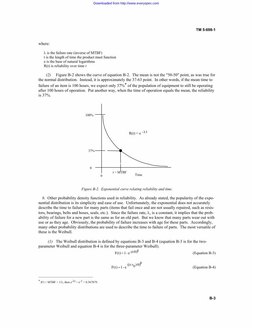
TM 5-698-1

B-3

where: O�is the failure rate (inverse of MTBF) t is the length of time the product must function e is the base of natural logarithms R(t) is reliability over time t (2) Figure B-2 shows the curve of equation B-2. The mean is not the "50-50" point, as was true for the normal distribution. Instead, it is approximately the 37-63 point. In other words, if the mean time to failure of an item is 100 hours, we expect only 37%* of the population of equipment to still be operating after 100 hours of operation. Put another way, when the time of operation equals the mean, the reliability is 37%.

Figure B-2. Exponential curve relating reliability and time. b. Other probability density functions used in reliability. As already stated, the popularity of the expo-nential distribution is its simplicity and ease of use. Unfortunately, the exponential does not accurately describe the time to failure for many parts (items that fail once and are not usually repaired, such as resis-tors, bearings, belts and hoses, seals, etc.). Since the failure rate, O, is a constant, it implies that the prob-ability of failure for a new part is the same as for an old part. But we know that many parts wear out with use or as they age. Obviously, the probability of failure increases with age for these parts. Accordingly, many other probability distributions are used to describe the time to failure of parts. The most versatile of these is the Weibull. (1) The Weibull distribution is defined by equations B-3 and B-4 (equation B-3 is for the two-parameter Weibull and equation B-4 is for the three-parameter Weibull).

ET )(t/-e - 1 )t(F (Equation B-3)

ET

])/0t-[(t-

e - 1 )t(F (Equation B-4) * If t = MTBF = 1/O, then e-Ot = e-1 = 0.367879.

Time

100%

0 0

t = MTBF

37%

R(t) = e O�- t


TM 5-698-1

B-4

(2) The Weibull distribution can provide accurate estimates of reliability with few samples, renders simple and useful graphical results, provide clues to physics of failure, and can represent many distribu-tions. When E is equal to 1, the Weibull is exactly equal to the exponential distribution. When, E is 3.44, the Weibull is approximately the normal distribution. c. Applicability of the exponential to systems. Although the exponential is often inappropriate for parts (i.e., items that fail once and are discarded), it is often applicable to systems. The reason is that systems are made of many parts, each with different failure characteristics. As parts fail, they are replaced. After some time, the system has parts of varying "ages". The net result is that the times between failures of the system are exponentially distributed. This behavior of system is described by Drenick's Theorem. B-4. Failure rate data How do we determine the failure rate of a specific product or component? Two methods are used. a. Method 1 - Comparable product. In the first method, we use failure rate data for a comparable product(s) already in use. This method has two underlying assumptions. First, the product in use is com-parable to the new product. Second, the principle of transferability applies. The principle of transferabil-ity states that (failure rate) data from one product can be used to predict the reliability of a comparable product. b. Method 2 – Testing. The other method of determining failure rate data is through testing of the product or its components. Although, theoretically, this method should be the "best" one, it has two dis-advantages. First, predictions are needed long before prototypes or pre-production versions of the product are available for testing. Second, the reliability of some components is so high that the cost of testing to measure the reliability in a statistically valid manner would be prohibitive. Usually, failure rate data from comparable products are used in the early development phases of a new product and supplemented with test data when available. B-5. Calculating reliability If the time, t, over which a product must operate and its failure rate, O, are known, then the reliability of the product can be calculated using equation B-2. If the information is known for individual subsystems or components, then the reliability of each can be calculated and the results used to calculate the reliabil-ity of the product. For example, consider the product represented by the reliability block diagram (RBD) in figure B-3. a. Series calculation. Components A, B, and C are said to be in series, which means all three must operate for the product to operate. Since the components are in series, we could find the reliability of each component using equation B-2 and multiply them as follows: 0.9900 x 0.9851 x 0.9925 = 0.9680. Alternatively, the product reliability can be found by simply adding together the failure rates of the com-ponents and substituting the result in equation B-4. The product failure rate is 0.001000 + 0.001500 + 0.000750 = 0.003250. The reliability is: 0.9680 e R(t) 10 x -0.003250


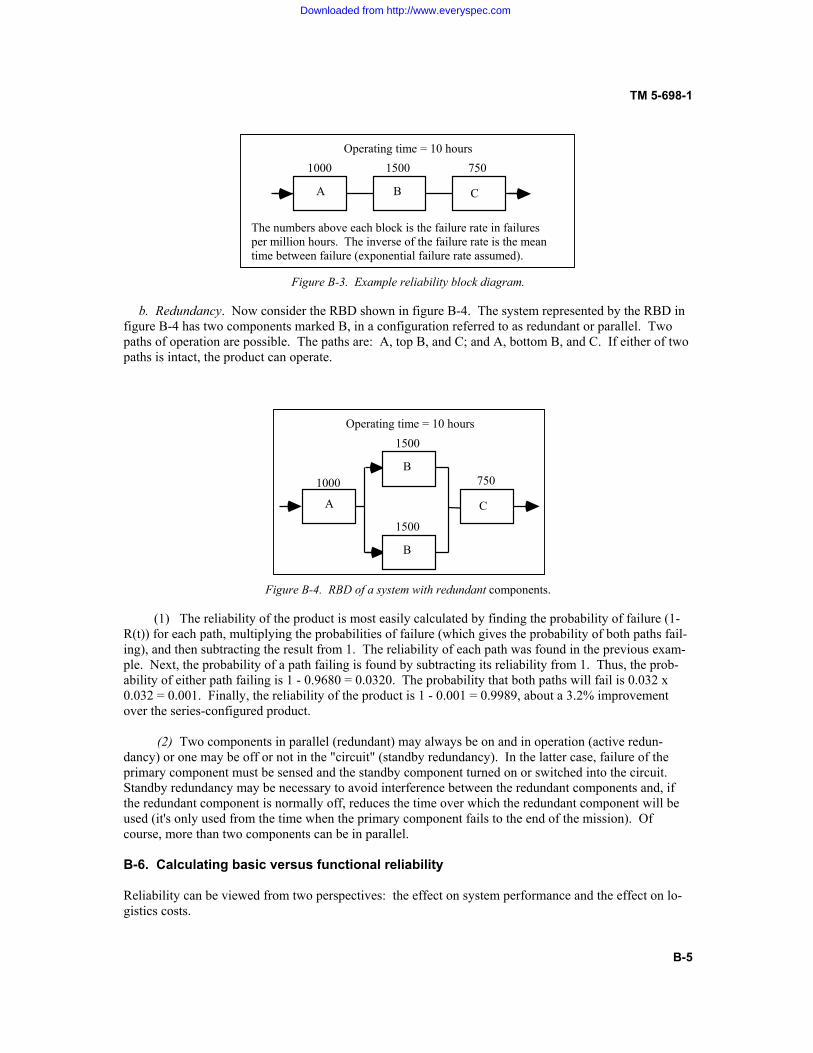
TM 5-698-1

B-5

Figure B-3. Example reliability block diagram. b. Redundancy. Now consider the RBD shown in figure B-4. The system represented by the RBD in figure B-4 has two components marked B, in a configuration referred to as redundant or parallel. Two paths of operation are possible. The paths are: A, top B, and C; and A, bottom B, and C. If either of two paths is intact, the product can operate.

Figure B-4. RBD of a system with redundant components. (1) The reliability of the product is most easily calculated by finding the probability of failure (1-R(t)) for each path, multiplying the probabilities of failure (which gives the probability of both paths fail-ing), and then subtracting the result from 1. The reliability of each path was found in the previous exam-ple. Next, the probability of a path failing is found by subtracting its reliability from 1. Thus, the prob-ability of either path failing is 1 - 0.9680 = 0.0320. The probability that both paths will fail is 0.032 x 0.032 = 0.001. Finally, the reliability of the product is 1 - 0.001 = 0.9989, about a 3.2% improvement over the series-configured product. (2) Two components in parallel (redundant) may always be on and in operation (active redun-dancy) or one may be off or not in the "circuit" (standby redundancy). In the latter case, failure of the primary component must be sensed and the standby component turned on or switched into the circuit. Standby redundancy may be necessary to avoid interference between the redundant components and, if the redundant component is normally off, reduces the time over which the redundant component will be used (it's only used from the time when the primary component fails to the end of the mission). Of course, more than two components can be in parallel. B-6. Calculating basic versus functional reliability Reliability can be viewed from two perspectives: the effect on system performance and the effect on lo-gistics costs.

A C

1000 750

B

1500

B

1500Operating time = 10 hours

A B C

1000 1500 750

The numbers above each block is the failure rate in failures per million hours. The inverse of the failure rate is the mean time between failure (exponential failure rate assumed).

Operating time = 10 hours


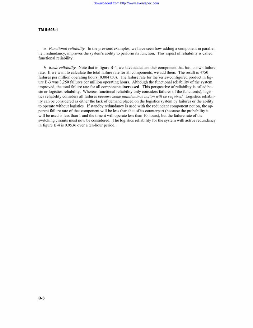
TM 5-698-1

B-6

a. Functional reliability. In the previous examples, we have seen how adding a component in parallel, i.e., redundancy, improves the system's ability to perform its function. This aspect of reliability is called functional reliability. b. Basic reliability. Note that in figure B-4, we have added another component that has its own failure rate. If we want to calculate the total failure rate for all components, we add them. The result is 4750 failures per million operating hours (0.004750). The failure rate for the series-configured product in fig-ure B-3 was 3,250 failures per million operating hours. Although the functional reliability of the system improved, the total failure rate for all components increased. This perspective of reliability is called ba-sic or logistics reliability. Whereas functional reliability only considers failures of the function(s), logis-tics reliability considers all failures because some maintenance action will be required. Logistics reliabil-ity can be considered as either the lack of demand placed on the logistics system by failures or the ability to operate without logistics. If standby redundancy is used with the redundant component not on, the ap-parent failure rate of that component will be less than that of its counterpart (because the probability it will be used is less than 1 and the time it will operate less than 10 hours), but the failure rate of the switching circuits must now be considered. The logistics reliability for the system with active redundancy in figure B-4 is 0.9536 over a ten-hour period.


TM 5-698-1

C-1

APPENDIX C

POINT ESTIMATES AND CONFIDENCE BOUNDS

C-1. Introduction to point estimates and confidence bounds Predicting reliability and maintainability is necessary because both characteristics are very difficult to measure, especially early in a development program. Some experts even deny that they can be measured at all. Without going into the philosophical and mathematical theories on which these experts base this denial, suffice it to say that predictions continue to be used in most every product development program. a. What is a prediction? Mathematically speaking, predictions are estimates of the true values of the parameters of any probability distribution. R&M, at least in part, are probability concepts. Reliability can be stated as the probability that a product will operate successfully under given conditions. Maintainability can be stated as the probability of completing a repair within a certain time under given conditions. If we observed the results of operating an entire population of a product in a given year, we could divide the number of failures by total attempted operations and determine the reliability of the product in that year after the fact. This "measurement" is not made to try and tell us what will happen next year or what would have happened in the year in question had only half the products been operated - it is not a prediction. Probability, on the other hand, is that branch of mathematics that allows statements to be made about a population based only on a sample of the population or when we try to predict before the fact the outcome of events. These predictions are estimations of the "truth." b. Types of estimates. Two kinds of estimation can be made: point estimates and interval estimates. (1) Point estimates. A point estimate is, as implied by the title, a single number that is an estimate of the distribution parameter in which we are interested. For example, on the basis of analysis or test, we might estimate the reliability to be 95%. How much confidence do we have in the estimate? It depends on the information used to make the estimate. If we used only analytical methods of arriving at the estimate (i.e., no actual testing performed), it would depend on how much the new product resembled the old product(s) from which the data used in the analysis were derived. If we had one test that was the basis for the estimate, we could be 50% sure that the true reliability is higher or lower than our estimate. Finally, if we test 100 products (out a larger total population), it seems intuitive that we could be more confident in our estimate than when we tested only one product. (a) As our sample size increases, we can make estimates in which we can have a higher confidence. Unfortunately, the subject of confidence is a bit more complex than that. For example, take the case where we have a sample of 100 products to test. Suppose that 10 failures occur. We could estimate the reliability to be 10/100 or 90%. We could also estimate it as 85% or 75%. How can that be? Well, the 90% figure is a point estimate in which we can be 50% confident. If we want to be more confident, say 95% confident that the true value is equal to or higher than the estimate, our estimate must be more conservative.


TM 5-698-1

C-2

(b) The reader might wonder what is wrong with just using a point estimate. Nothing is "wrong" with using a point estimate. But a point estimate isn't discriminating; it tells us nothing about the risk involved with the estimate. And there is always the risk that our estimate of reliability is optimistic, i.e., too high (customers don't care, at least in theory, if it's too low, i.e., conservative). Consider the example estimates in table C-1. From the table, one can understand why a point estimate is not discriminating! Most people would more readily accept the point estimate made using 1000 products than that made with only 10.

Table C-1. Point estimates for different sample sizes

Size of Sample (or number of tests)

Number of Failures

Point Estimate of Reliability

10 1 90% 100 10 90% 1000 100 90%

(2) Interval estimates. An interval estimate is one in which we calculate a range of values and can state the probability of the true value of the parameter being estimated being contained in the interval. The lower and upper values of the interval are called lower and upper confidence limits, respectively. The confidence level is the probability that the range or interval of values actually includes the true value of reliability. A confidence bound can be two-sided or one-sided. A two-sided bound can be compared to a tolerance. Most of us are familiar with a measurement that is stated, for example, as 12 feet ± 0.01 feet. A two-sided bound on a reliability estimate of 95% might be ±2.1%, at 95 confidence. In other words, we are 95% confident that the interval of 92.9% to 97.1% includes the true reliability. We may, however, only be interested in the lower limit. A one-sided confidence bound would be stated as, for example, "we are 95% confident that the true reliability is greater than 90%." In this case, we are not worried about how much higher it may be. If we are trying to determine if a contractor has met (or exceeded) the reliability requirement, the one-sided confidence bound is sufficient. If we want to plan a spares buy based on the reliability of the product, the two-sided bound should be used. c. Estimation and confidence are topics filling entire chapters of textbooks. The discussion herein is necessarily simplified and abbreviated. For a more rigorous and mathematically accurate treatment of estimation and confidence, the reader is directed to "Practical Statistical Analysis for the Reliability Engineer (SOAR-2)," The Reliability Analysis Center, Kieron A. Dey, 1983. (Available from the Reliability Analysis Center: 1-800-526-4802), or "Methods for Statistical Analysis of Reliability and Life Test Data," Nancy R. Mann, Ray E. Schafer, and Nozer D. Singpurwalla, John Wiley and Sons, Inc., Somerset, NJ, 1974, or any good text on probability and statistics.


TM 5-698-1

D-1

APPENDIX D

FACTORS INFLUENCING FIELD MEASURES OF RELIABILITY

D-1. Inherent reliability versus operational reliability The reliability achieved by diligent attention to failure modes and mechanisms during design and manufacture is defined as inherent reliability. The reliability actually observed during operation of the system in its intended environment is defined as operational reliability. a. Inherent reliability. Inherent reliability is by definition the level of reliability inherent in the system as designed and manufactured. All failures are due to inherent weaknesses in the design, flaws in the materials, or defects from the manufacturing processes. The level of inherent reliability achieved is determined through analysis and test. Although in applying analytical methods and in testing the system (the "actual" system or prototypes), the design and development team attempts to simulate the actual operating environment, it is difficult if not impossible to account for some aspects of operation. b. Operational reliability. Operational reliability is the measure a customer or user of a system uses. Whenever a system fails to perform its function(s) or requires maintenance, the customer will count such events as failures, regardless of the cause. Inherent weaknesses in the design, flaws in the materials, and defects from the manufacturing processes will cause such failures, but so will maintenance errors, improper operation, and changes in operating concept. In addition, if the operating environment is substantively different from that defined during design, more failures or failure modes may occur than were addressed during design and manufacturing. Consequently, operational reliability can never be higher than inherent reliability and is usually lower. D-2. Accounting for the differences We can account for the differences between design and operational reliability. We can do so in two ways: the way we design and develop procedures, and the way in which we develop design requirements. a. Design and procedure. Recognizing that humans make mistakes, we can apply design techniques that minimize the chance of human error. For example, we can design mating parts to mate in only one way, preventing maintenance personnel from making an incorrect connection. We can design displays that are easy to read and use conventional symbols. We can design controls using standard orientation (e.g., turn right to shut off a valve). In a similar manner, we can write procedures that are clear, concise, and logical. Such attention to the human element during design can minimize the opportunity for human error. b. Design requirements. If the customer needs a operational reliability of 1000 hours Mean Time Between Failures (MTBF) for a system, we cannot use 1000 hours as our design requirement. If we did so, and missed one failure mode due to our inexact understanding of the operating environment, we would not meet the operational reliability requirement. We must, therefore, design to a higher level. Of course, we should not set an arbitrarily high inherent reliability requirement. To do so would drive up costs unnecessarily. A commonly used


TM 5-698-1

D-2

approach for setting the inherent reliability requirement is to use past experience. If experience with previous systems indicates that the operational reliability runs 10%-15% lower than what was measured during design and manufacture, then, as a rule of thumb, the inherent reliability requirement for new systems should be 12% higher than the operational reliability requirement. For example, if the inherent reliability for past systems was 1,000 hours MTBF and the observed operational reliability was only 850 hours (15% less), and the operational reliability requirement for a new system is 1,000 hours, the inherent reliability requirement must be about 11.8% higher or 1,180 hours. If we achieve this level of inherent reliability, then we can expect our operational reliability to be 1180 - (15% x 1180) = 1,003 hours.


TM 5-698-1

G-1

GLOSSARY

1. Glossary

-A- ACTIVE TIME: That time during which an item is in an operational inventory. AFFORDABILITY: Affordability is a measure of how well customers can afford to purchase, operate, and maintain a product over its planned service life. Affordability is a function of product value and product costs. It is the result of a balanced design in which long-term support costs are considered equally with near-term development and manufacturing costs. ALIGNMENT: Performing the adjustments that are necessary to return an item to specified operation. ALPHA (Į): The probability, expressed as a decimal that a given part will fail in the identified mode. The sum of all alphas for a component will equal one (1). AVAILABILITY: The instantaneous probability that a component will be up.

AVAILABILITY, INHERENT (Ai). The instantaneous probability that a component will be up. Ai

considers only downtime for repair due to failures. No logistics delay time, preventative maintenance, etc. is included.

AVAILABILITY, OPERATIONAL (Ao). Ao is the instantaneous probability that a component will be up but differs from inherent availability in that it includes ALL downtime. Included is downtime for both corrective maintenance and preventative maintenance, including any logistics delay time.

-B- BETA (ȕ): The conditional probability that the effect of a failure mode will occur, expressed as a deci-mal. If a failure is to occur, what is the probability that the outcome will occur. Block Diagrams: Availability block diagrams and reliability block diagrams are visual representations of the interactions between contributors to reliability, availability, and maintainability. Each block tends to represent a physical component in the system and its associated reliability/availability. Boolean Algebra: Boolean algebra is a method of calculating system availability based on logical inter-actions between components. AND and OR operators define mathematical operations. BROWNOUT: Occurs during a power failure when some power supply is retained, but the voltage level is below the minimum level specified for the system. A very dim household light is a symptom of a brownout.

-C- CALIBRATION: A comparison of a measuring device with a known standard and a subsequent adjust-ment to eliminate any differences. Not to be confused with alignment.


TM 5-698-1

G-2

CANNOT DUPLICATE (CND): A situation when a failure has been noted by the operator but cannot be duplicated by maintenance personnel attempting to correct the problem. Also see Retest OK. CHECKOUT: Tests or observations of an item to determine its condition or status. COMPENSATING PROVISION: Actions available or that can be taken to negate or reduce the effect of a failure on a system. COMPONENT: A piece of electrical or mechanical equipment viewed as an entity for the purpose of reliability evaluation CONDITION-BASED PM: Maintenance performed to assess an item's condition and performed as a result of that assessment. Some texts use terms such as predictive maintenance and on-condition. The definition of condition-based PM used herein includes these concepts. In summary, the objectives of condition-based PM are to first evaluate the condition of an item, then, based on the condition, either de-termine if a hidden failure has occurred or determine if a failure is imminent, and then take appropriate action. Maintenance that is required to correct a hidden failure is, of course, corrective maintenance. CORRECTIVE ACTION: A documented design, process, procedure, or materials change implemented and validated to correct the cause of failure or design deficiency. CORRECTIVE MAINTENANCE (CM): All actions performed as a result of failure, to restore an item to a specified condition. Corrective maintenance can include any or all of the following steps: Lo-calization, Isolation, Disassembly, Interchange, Reassembly, Alignment and Checkout. COST: The expenditure of resources (usually expressed in monetary units) necessary to develop, ac-quire, or use a product over some defined period of time. CRITICALITY: A relative measure of the consequences of a failure mode and the frequency of its oc-currence. CRITICALITY ANALYSIS (CA): A procedure by which each potential failure mode is ranked accord-ing to the combined influence of severity and probability of occurrence.

-D- DEPENDABILITY: A measure of the degree to which an item is operable and capable of performing its required function at any (random) time during a specified mission profile, given item availability at the start of the mission. (Item state during a mission includes the combined effects of the mission-related system R&M parameters but excludes non-mission time; see availability). DETECTABLE FAILURE: Failures at the component, equipment, subsystem, or system (product) level that can lie identified through periodic testing or revealed by an alarm or an indication of an anomaly. DETECTION METHOD: The method by which a failure can be discovered by the system operator un-der normal system operation or by a maintenance crew carrying out a specific diagnostic action. DIAGNOSTICS: The hardware, software, or other documented means used to determine that a malfunc-tion has occurred and to isolate the cause of the malfunction. Also refers to "the action of detecting and isolating failures or faults."


TM 5-698-1

G-3

DOWNTIME: That element of time during which an item is in an operational inventory but is not in condition to perform its required function.

-E- EFFECTIVENESS: The degree to which PM can provide a quantitative indication of an impending functional failure, reduce the frequency with which a functional failure occurs, or prevent a functional failure. END EFFECT: The consequence a failure mode has upon the operation, function or status at the highest indenture level. EQUIPMENT: A general term designating an item or group of items capable of performing a complete function.

-F- FAILURE (f). The termination of the ability of a component or system to perform a required function. FAILURE, CATASTROPHIC: A failure that causes loss of the item, human life, or serious collateral damage to property. FAILURE, HIDDEN: A failure that is not evident to the operator; that is, it is not a functional failure. A hidden failure may occur in two different ways. In the first, the item that has failed is one of two or more redundant items performing a given function. The loss of one or more of these items does not result in a loss of the function. The second way in which a hidden failure can occur is when the function per-formed by the item is normally inactive. Only when the function is eventually required will the failure become evident to the operator. Hidden failures must be detected by maintenance personnel. FAILURE, INTERMITTENT: Failure for a limited period of time, followed by the item's recovery of its ability to perform within specified limits without any remedial action. FAILURE, RANDOM: A failure, the occurrence of which cannot be predicted except in a probabilistic or statistical sense. FAILURE ANALYSIS: Subsequent to a failure, the logical systematic examination of an item, its con-struction, application, and documentation to identify the failure mode and determine the failure mecha-nism and its basic course. FAILURE CAUSE: The physical or chemical processes, design defects, quality defects, part misappli-cation or other processes which are the basic reason for failure or which can initiate the physical process by which deterioration proceeds to failure. FAILURE EFFECT: The consequence(s) a failure mode has on the operation, function, or status of an item. Failure effects are typically classified as local, next higher level, and end. FAILURE MECHANISM: The physical, chemical, electrical, thermal or other process which results in failure.


TM 5-698-1

G-4

FAILURE MODE: The way in which a failure is observed, describes the way the failure occurs, ie., short, open, fracture and excessive wear.. FAILURE MODE AND EFFECTS ANALYSIS (FMEA): A procedure by which each potential fail-ure mode in a product (system) is analyzed to determine the results or effects thereof on the product and to classify each potential failure mode according to its severity or risk probability number. FAILURE MODES, EFFECTS, AND CRITICALITY ANALYSIS (FMECA): The term is used to emphasize the classifying of failure modes as to their severity (criticality). FAILURE RATE (Ȝ): The mean (arithmetic average, also known as the forced outage rate) number of failures of a component and/or system per unit exposure time. The most common unit in reliability analy-ses is hours (h).However, some industries use failures per year (f/y) which is denoted by the symbol (Ȝy). FAILURE REPORTING AND CORRECTIVE ACTION SYSTEM (FRACAS): A closed-loop sys-tem for collecting, analyzing, and documenting failures and recording any corrective action taken to eliminate or reduce the probability of future such failures. FALSE ALARM: A fault indicated by BIT or other monitoring circuitry where no fault can be found or confirmed. FAULT: Immediate cause of failure (e.g., maladjustment, misalignment, defect, etc.). FAULT DETECTION (FD): A process that discovers the existence of faults. FAULT ISOLATION (FI): The process of determining the location of a fault to the indenture level necessary to affect repair. FAULT TREE ANALYSIS: An analysis approach in which each potential system failure is traced back to all faults that could cause the failure. It is a top-down approach, whereas the FMEA is a bottom-up approach. FINITE ELEMENT ANALYSIS (FEA): A modeling technique (normally a computer simulation) used to predict the material response or behavior of the device or item being modeled. FEA can describe mate-rial stresses and temperatures throughout the modeled device by simulating thermal or dynamic loading conditions. It can be used to assess mechanical failure mechanisms such as fatigue, rupture, creep, and buckling. FUNCTIONAL TEST: An evaluation of a product or item while it is being operated and checked under limited conditions without the aid of its associated equipment in order to determine its fitness for use.

-H- HOURS DOWNTIME PER YEAR (Hrdt/Year). Average hours the item is expected to be not func-tional in a one year period, caused by both preventative maintenance and failures. This includes any lo-gistics delay time.

-I- INDENTURE LEVELS: The levels which identify or describe the relative complexity of an assembly or function.


TM 5-698-1

G-5

ISOLATION: Determining the location of a failure to the extent possible, by the use of accessory equip-ment. ITEM CRITICALITY NUMBER (Cr): A relative measure of consequence of an item failure and its frequency of occurrence. This factor is not applicable to a qualitative analysis.

-L- LEVELS OF MAINTENANCE: The division of maintenance, based on different and requisite techni-cal skill, which jobs are allocated to organizations in accordance with the availability of personnel, tools, supplies, and the time within the organization. Typical maintenance levels are organizational, intermedi-ate, and depot. LIFE CYCLE COST (LCC): The sum of acquisition, logistics support, operating, and retirement and phase-out expenses. LIFE CYCLE PHASES: Identifiable stages in the life of a product from the development of the first concept to removing the product from service and disposing of it. Within the Department of Defense, four phases are formally defined: Concept Exploration; Program Definition and Risk Reduction; Engi-neering and Manufacturing Development; and Production, Deployment, and Operational Support. Al-though not defined as a phase, demilitarization and disposal is defined as those activities conducted at the end of a product's useful life. Within the commercial sector, various ways of dividing the life cycle into phases are used. One way of doing this is as follows: Customer Need Analysis, Design and Develop-ment, Production and Construction, Operation and Maintenance, and Retirement and Phase-out. LINE REPLACEABLE UNIT (LRU): A unit designed to be removed upon failure from a larger entity (product or item) in the operational environment, normally at the organizational level. LOCAL EFFECT: The consequence a failure mode has on the operation, function or status of the spe-cific item being analyzed. LOCALIZATION: Determining the location of a failure to the extent possible, without using accessory test equipment. LOGISTIC DELAY TIME: That element of downtime during which no maintenance is being accom-plished on the item because of either supply or administrative delay. LOGISTICS SUPPORT: The materials and services required to enable the operating forces to operate, maintain, and repair the end item within the maintenance concept defined for that end item.

-M- MAINTAINABILITY: The relative ease and economy of time and resources with which an item can be retained in, or restored to, a specified condition when maintenance is performed by personnel having specified skill levels, using prescribed procedures and resources, at each prescribed level of maintenance and repair. Also, the probability that an item can be retained in, or restored to, a specified condition when maintenance is performed by personnel having specified skill levels, using prescribed procedures and re-sources, at each prescribed level of maintenance and repair. MAINTENANCE: All actions necessary for retaining an item in or restoring it to a specified condition.


TM 5-698-1

G-6

MAINTENANCE ACTION: An element of a maintenance event. One or more tasks (i.e., fault local-ization, fault isolation, servicing and inspection) necessary to retain an item’s condition or restore it to a specified condition. MAINTENANCE CONCEPT: A description of the planned general scheme for maintenance and sup-port of an item in the operational environment. It provides a practical basis for design, layout, and pack-aging of the system and its test equipment. It establishes the scope of maintenance responsibility for each level of maintenance and the personnel resources required to maintain the system. MAINTENANCE DOWNTIME (Mdt). The total downtime for preventative maintenance (including logistics delay time, which includes spare parts availability, crew availability, etc) for a given period,Tp. (hours). MAINTENANCE EVENT: One or more maintenance actions required to effect corrective and preven-tive maintenance due to any type of failure or malfunction, false alarm or scheduled maintenance plan. MAINTENANCE TASK: The maintenance effort necessary for retaining an item in, or chang-ing/restoring it to a specified condition. MAINTENANCE TIME: An element of downtime that excludes modification and delay time. MEAN DOWNTIME (MDT). The average downtime caused by preventative and corrective mainte-nance, including any logistics delay time. This is synonymous with mean time to restore system (MTTRS) as found in some publications. MEAN TIME BETWEEN FAILURES (MTBF). The mean exposure time between consecutive fail-ures of a component. MTBF is a require measurement used for calculating inherent availability. It can be estimated by dividing the exposure time by the number of failures in that period. MEAN TIME BETWEEN MAINTENANCE (MTBM). The average time between all maintenance events that cause downtime, both preventative and corrective maintenance, and also includes any associ-ated logistics delay time.

MEAN TIME TO FAILURE (MTTF): The mean exposure time between consecutive repairs (or instal-lations) of a component and the next failure of that component. MTTF is commonly found for non-repairable items such as fuses or bulbs, etc. MEAN TIME TO MAINTAIN (MTTM). The average downtime for preventative maintenance. This includes any logistics delay time. MEAN TIME TO REPAIR (MTTR). The mean time to replace or repair a failed component. Logistics delay time associated with the repair, such as parts acquisitions, crew mobilization, are not included. It can be estimated by dividing the summation of repair times by the number of repairs and, therefore, is practically the average repair time. The most common unit in reliability analyses is hours (h/f).

-N- NEXT HIGHER LEVEL EFFECT: The consequence a failure mode has on the operation, functions, or status of the items in the next higher indenture level above the specific item being analyzed.


TM 5-698-1

G-7

-O- ON-CONDITION MAINTENANCE: See Condition-based PM. ONE-LINE DIAGRAM: A one-line diagram is a drawing of an electrical or mechanical system that shows how the parts interact. It shows paths of electrical flow, water flow, gas flow, etc. It will also list system component and component sizes. OPERATING AND SUPPORT (O&S) COSTS: Those costs associated with operating and supporting (i.e., using) a product after it is purchased or fielded. OPERATIONAL READINESS: The ability of a military unit to respond to its operation plan(s) upon receipt of an operations order. (A function of assigned strength, item availability, status, or supply, train-ing, etc.).

-P- PREDICTED: That which is expected at some future time, postulated on analysis of past experience and tests. PREDICTIVE MAINTENANCE: See Condition-based PM. PREVENTATIVE MAINTENANCE (PM): All actions performed in an attempt to retain an item in a specified condition. These actions may or may not result in downtime for the component, and may or may not be performed on a fixed interval.

-Q- QUALITATIVE ANALYSIS: A means of conducting an analysis without data. Team member subjec-tively rank probabilities of occurrence, typically 1-10, in place of failure rates. QUANTITATIVE ANALYSIS: An analysis that is supported with data. Data is available for assigning failure rates and failure mode probabilities.

-R- REASSEMBLY: Assembling the items that were removed during disassembly and closing the reassem-bled items. REDUNDANCY: The existence of more than one means for accomplishing a given function. Each means of accomplishing the function need not necessarily be identical. RELIABILITY (R(t)). The probability that a component can perform its intended function for a speci-fied time interval (t) under stated conditions. This calculation is based on the exponential distribution. RELIABILITY-CENTERED MAINTENANCE (RCM): A disciplined logic or methodology used to identify preventive and corrective maintenance tasks to realize the inherent reliability of equipment at a minimum expenditure of resources, while ensuring safe operation and use. REPAIR DOWNTIME (Rdt). The total downtime for corrective maintenance (excluding logistics delay time) for a given Tp (hours).


TM 5-698-1

G-8

REPAIR LOGISTICS TIME (Rlt). The total logistics delay time for corrective maintenance for a given Tp (hours). RETEST OK (RTOK): A situation where a failure was detected on the system, either through inspec-tion or testing, but no fault can be found in the item that was eventually removed for repair at a field or depot location. Also see Cannot Duplicate.

-S- SECONDARY EFFECTS: The results or consequences indirectly caused by the interaction of a dam-age mode with a system, subsystem or component of the system. SEVERITY: Considers the worst possible consequence of a failure classified by the degree of injury, property damage, system damage and mission loss that could occur. SCHEDULED MAINTENANCE: Periodic prescribed inspection and/or servicing of products or items accomplished on a calendar, mileage or hours of operation basis. Included in Preventive Maintenance. SERVICING: The performance of any act needed to keep an item in operating condition, (i.e. lubricat-ing, fueling, oiling, cleaning, etc.), but not including preventive maintenance of parts or corrective main-tenance tasks. SINGLE-POINT FAILURE: A failure of an item that causes the system to fail and for which no redun-dancy or alternative operational procedure exists. SUBSYSTEM: A combination of sets, groups, etc. that performs an operational function within a prod-uct (system) and is a major subdivision of the product. (Example: Data processing subsystem, guidance subsystem). SYSTEM. A group of components connected or associated in a fixed configuration to perform a speci-fied function. SYSTEM DOWNTIME: The time interval between the commencement of work on a system (product) malfunction and the time when the system has been repaired and/or checked by the maintenance person, and no further maintenance activity is executed.

-T- TESTABILITY: A design characteristic that allows status (operable, inoperable, or degraded) of an item to be determined and the isolation of faults within the item to be performed in a timely manner. TOTAL DOWNTIME EVENTS (Tde): The total number of downtime events (including scheduled maintenance and failures) during the Tp. TOTAL FAILURES (Tf). The total number of failures during the Tp. TOTAL PERIOD (Tp). The calendar time over which data for the item was collected. TOTAL MAINTENANCE ACTIONS (Tma). The total number of preventative maintenance actions which take the component down during the Tp


TM 5-698-1

G-9

TOTAL SYSTEM DOWNTIME: The time interval between the reporting of a system (product) mal-function and the time when the system has been repaired and/or checked by the maintenance person, and no further maintenance activity is executed.

-U- UNSCHEDULED MAINTENANCE: Corrective maintenance performed in response to a suspected failure. UPTIME: That element of ACTIVE TIME during which an item is in condition to perform its required functions. (Increases availability and dependability). USEFUL LIFE: The number of life units from manufacture to when the item has an unrepairable failure or unacceptable failure rate. Also, the period of time before the failure rate increases due to wearout.

-W- WEAROUT: The process that results in an increase of the failure rate or probability of failure as the number of life units increases.

-Y- YEAR (y): The unit of time measurement approximately equal to 8765.81277 hours (h). Any rounding of this value will have adverse effects on analyses depending on the magnitude of that rounding. 8766 is used commonly as it is the result of rounding to 365.25×24 (which accounts for a leap year every 4th year). 8760, which is 365×24, is the most commonly used value in the power reliability field. By conven-tion, 8760 will be used throughout this document.


TM 5-698-1 The proponent agency of this publication is the Chief of Engineers, United States Army. Users are invited to send comments and suggested improvements on DA Form 2028 (Recommended Changes to Publications and Blank Forms) directly to HQUSACE, (ATTN: CEMP-OS-P), Washington, DC 20314-1000.

Distribution:

To be distributed in accordance with Initial Distribution Number (IDN) 344746, requirements for non-equipment TM 5-698-1.

By Order of the Secretary of the Army:

PETER J. SCHOOMAKER General, United States Army

Chief of Staff Official:

JOYCE E. MORROW Administrative Assistant to the

Secretary of the Army


PIN: 080730-000


RELIABILITY/AVAILABILITY OF ELECTRICAL & MECHANICAL ...

Documents

Transcript of RELIABILITY/AVAILABILITY OF ELECTRICAL & MECHANICAL ...