Reliability Improvement and Assessment of Safety Critical ...

Reliability Improvement and Assessment of Safety Critical Software

by

Yu Sui

Submitted to the Department of Nuclear Engineering and Depart-ment of Electrical Engineering and Computer Science in partial ful-

fillment of the requirements for the degree of

Master of Science

at the

MASSACHUSETTS INSTITUTE OF TECHNOLOGY

.May 20, 1998

© Massachusetts Institute of Technology, 198. All Rights Reserved

A uthor ....................................... ..................................... .............. .... .Nuclear Engineering Department

May 20, 1998

Certified by ... ....................... . ..................... ........ .. .. .

M. W. Gola or of Nuclear Engineeringesis Co-Supervisor

C ertified b y ................... ...................... ...............................................................D. Jackson

Associate Professor of Electrical Engineering and Computer ScienceThesis Co-Supervisor

Accepted byL. M. Lidsky, Professor of Nuclear Engineering

Chairman, Departmental Committee-on Graduate Students

Accepted by .................... ..-............A.C. Smith

Professor of Electrical Engineering and Computer ScienceChairman, Departmental Committee on Graduate Students

4 .'

Reliability Improvement and Assessment of Safety-Critical Software

by

Yu Sui

Submitted to the Department of Nuclear Engineering and the Department of Electrical Engineering andComputer Science

on May 20, 1998, in partial fulfillment of the requirements for the degree of

MASTER OF SCIENCE

Abstract

In order to allow the introduction of safety-related Digital Instrumentation and Control(DI&C) systems in nuclear power plants, the software used by the systems must be demonstratedto be highly reliable. The most widely used and most powerful method for ensuring high softwarequality and reliability is testing. An integrated methodology is developed in this thesis forreliability assessment and improvement of safety critical software through testing. The

methodology is based upon input domain-based reliability modeling and structural testingmethod. The purpose of the methodology is twofold: Firstly it can be used to control the testingprocess. The methodology provides path selection criteria and stopping criteria for the testingprocess with the aim to achieve maximum reliability improvement using available testingresources. Secondly, it can be used to assess and quantify the reliability of the software after thetesting process. The methodology provides a systematic mechanism to quantify the reliability andestimate uncertainty of the software after testing.

Thesis Supervisor: M.W. GolayTitle: Professor of Nuclear Engineering

Thesis Supervisor: D. JacksonTitle: Associate Professor of Electrical Engineering and Computer Science

Acknowledgments

The author would like to acknowledge ABB-Combustion Engineering for their generouspermission for us to use their proprietary software and supporting documents in our case study.Special thanks go to Michael Novak, the primary contact-person at ABB-CE, for his comments,clear focus of requirements upon our research.

Thanks also go to Hamilton Technology Inc. for supplying the 001 system for use in theproject. Special thanks go to Ronald Hackler for his technical guidance in using the wonderfulfeatures of the 001 system.

Table of Contents

A bstract ................................................................................................................... 2Acknowledgments.................................................................................................... 3Table of Contents.................................................................................................... 4List of Figures.................................................................................................... 8List of Tables ................................................................................ .......... 9

1. Introduction.......................................................................... ................................. 10

1.1 M otivation of the Study......................................... ......................... ....................... 10

1.2 G oal of the Study......................... ..... ... ..... . ..... ............ ........... 12

1.3 O rganization of the Thesis.......................................... ... ................................... 13

2. Study of the Current Practice .............................................................................. 14

2.1 Introduction................................ 14

2.2 Fundamentals of Reliability Theory........................................... .................... 14

2.2.1 Reliability M athematics.................................................... 15

2.2.2 Some Useful Definitions in Software Reliability Theory.............................. . 16

2.3 Software Reliability Growth Models................................ 17

2.3.1 Time Between Failure Models................................................. 18

2.3.2 Failure C ount M odels ............................................................... ......................... 20

2.3.3 Advantages and Limitations of Software Reliability Growth Models............. 22

2.4 Fault Seeding Models ........... .................................. 24

2.5 Input Domain-Based Reliability Models....................... ... ....................... 25

2.5.1 R andom T esting.. ............................................................ ................................. 26

2.5.2 Subdomain/Partition Testing............................................... ... 27

2.5.3 Advantages and Limitations of Input Domain-Based Models ........................... 29

3. The Integrated Methodology ................................................... 32

3.1 The Control Flowgraph............................. ... ....................... 32

3. 1.1 Elements of the Control Flowgraph ............................... 32

3.1.2 A n Illustrative Exam ple........................................... ................ ....................... 35

3.1.3 Som e U seful Term s................................................ .......................................... 38

3.2 The Underlying Software Reliability Model.................................... ............. 38

3.3 The Feasible Structured Path Testing M ethod......................................................... ... 41

3.3.1 M ethod O verview ......................................... ................................................... 42

3.3.2 M ethod D etails.................................................... ................................................ 42

3.3.3 M ethod A utom ation........................................................................................ 48

3.4 T he Estim ation of p ....................................................... . . .. . . . .. . . .. . . .. . . .. . . .. . .. .. . .. . .. . .. .. . .. . 51

3.4.1 The Estimation of the Operational Profile............................................ 51

3.4.2 The Estimation of pi Based upon the Operational Profile............................. 52

3.4.2.1 The Direct Integration Method................................ .............. 52

3.4.2.2 The Monte Carlo Method..................................... 54

3.4.2.2.1 The Application of the Monte Carlo Method............................... 54

3.4.2.2.2 Advantages and Limitations....................................55

3.4.2.2.3 Method Automation............................................ 56

3.5 Testing................................................................... 56

3.5.1 The General Testing Strategy.................................. ... 56

3.5.2 Testing Automation.........................................................58

3.6 The Estimation of 08 ................. ......................... .. ......... ........ ................................. 59

3.6.1 The Average Error Content per Path, e.......................... ................... 59

3.6.2 The General Strategy................................ ....................... 60

3.6.2.1 The Estimation of the 60 of the Tested Paths................................... 61

3.6.2.2 The Estimation of the Oi of the Untested Paths.................................. 63

3.6.3 The Estimation of 0 ........................................ ................... 64

3.6.3.1 The Estimation of 0 Using Software Metrics....................64

3.6.3.2 The Estimation of 0 Using the Bayesian Updating Method.................... 65

3.6.3.2.1 Mathematical Foundation.......................................... 65

3.6.3.2.2 Performance Analysis............................. ..... ................. 67

3.6.3.2.2.1 Failure Vs. No Failure ..................................... ......... 68

3.6.3.2.2.2 Number of Tested Paths................................... ...... ... 69

3.6.3.2.2.2.1 N o Failure Case..................... .................................... 69

3.6.3.2.2.2.2 W ith Failure Case................................... .......... 70

3.6.3.2.2.3 The Prior Distribution......................... .............. 71

3.6.3.2.2.3.1 No Failure Case..................................................... ...71

3.6.3.2.2.3.1 W ith Failure Case.......................................................... 72

3.6.3.2.2.4 A Brief Sum mary.......................... ........ ............................ 73

3.6.3.2.3 Advantages and Limitations............................................. 73

3.7 Summary of the M ethodology............................ ........................ 75

3.7.1 The General Application Strategy................................75

3.7.2 Some Useful Observations............................................... 76

3.7.3 Underlying Assumptions and Potential Applications................................... 78

3.7.4 A dvantages and Lim itations........................................... ............................. 79

4. A Case Study Using the Integrated Methodology................ ...... 81

4.1 Introduction.............................. ............. .................. 81

4.2 The Signal Validation Algorithm............................................................. 82

6

4.2.1 The Signal Validating Features............................................82

4.2.2 The Implementation of the SVA................... ..................... 83

4.3 The Testing Process................................ .. ............................ 84

4.3.1 Modular Testing........................................... .................................................... 84

4.3.2 Integrated Testing............................................................ .......................... 88

4.4 Testing Results Analysis.............................................................................................89

4 .5 C o nclusio ns............................. .............................................................................. 92

5. Conclusions and Future W ork .................................................. 93

5.1 Conclusions.............. ..................................................................................... 93

5.2 Future W ork .................................................................................................................... 94

References....................................................................................................................... 95

List of Figures

Figure 3.1 A process node.............................................................................................. 33

Figure 3.2 A decision node......................................................... .............................. 33

Figure 3.3 A junction node....................................... ................................................. 34

Figure 3.4 The pseudo programming language................................ ............. 35

Figure 3.5 Automatic Teller Machine (ATM) example code.......................................36

Figure 3.6 ATM example code and its flowgraph........................................................ 37

Figure 3.7 Flowgraph expanded to k iterations.......................... ... .............. 43

Figure 3.8 H orrible loops....................................................................................... 44

Figure 3.9 Flowgraph expansion with respect to transitional variables..........................46

Figure 3.10 Comparison of failure vs. no failure cases................................... 68

Figure 3.11 Posterior evolution when no failures occur...............................................69

Figure 3.12 Posterior evolution when failures occur............................... ........ 70

Figure 3.13 Sensitivity analysis when no failures occur.................................... 71

Figure 3.14 Sensitivity analysis when failures occur.................................. ..... 72

Figure 4.1 Module AverageGood FMap................................................ 86

Figure 4.2 Control flowgraph of the module AverageGood and its expansion............ 87

Figure 4.3 The prior distribution of the case study.................................. ........ 90

Figure 4.4 The posterior distribution of the case study................................................ 91

List of Tables

Table 4.1 Paths in module AverageGood..................................................................... 87

Chapter 1

Introduction

1.1 Motivation of the Study

In Nuclear Power Plants (NPPs), the current Instrumentation and Control (I&C) system is

based upon analog technologies. Analog devices are prone to aging problems, need to be

calibrated regularly, are becoming obsolescent and their replacement parts are more and more

difficult to find as the outside industries are quickly digitized. In safety critical systems, use of

digital computers provides many potential advantages including improved availability, easier

maintenance, reduced installation cost, ease of modification and potential for reuse. Many nuclear

utilities are trying to replace their obsolescent analog control systems with Digital

Instrumentation and Control (DI&C) systems. The next generation of NPPs in the United States is

expected to be completely computerized and have an integrated DI&C system.

Despite of all the advantages the DI&C system may offer, currently the acceptance of

DI&C system in the nuclear industry has been greatly retarded. The reason is mainly due to the

difficulties of verification and validation (V&V) of the digital control software, and the

difficulties of assessment of the reliability of the digital control software. The DI&C system

introduces new failure modes (i.e., software failures), into the control system. Unlike that of the

hardware, software failures are exclusively caused by design errors. They are common-cause

failures and can not be reduced by adopting redundancy principles. The most widely used and

most powerful method for attacking software design errors is testing. The software is tested

against its design specification, which is a part of the verification and validation process.

Comparing results of the test cases with the oracle can reveal errors in the software. If the

software can be exhaustively tested, its reliability can be proven to be unity. However, exhaustive

testing can seldom be achieved in practice due to the complexity of the software, the limited time

and resources available. Consequently two problems exist: How to control the testing process to

achieve maximum testing efficiency, i.e., to achieve maximum reliability improvement using the

limited testing resources; How to assess the reliability of the improved, while still not perfect

software after testing? Assessment and quantification of software reliability play a central role in

ensuring high software quality, which is especially important for the safety-critical control

software in nuclear industry applications. If the reliability of the software can be assessed and

quantified with high confidence, it can then be compared with that of the hardware, which can be

readily quantified using current technologies, to show that new digital systems are sufficiently

reliable. Wide acceptance of DI&C system and substantial improvements in nuclear power safety

and economics would be likely.

In the current practice, the most widely used models for software reliability assessment

and qualification are time domain-based software reliability growth models. For a given software,

an appropriate reliability growth model is first chosen for use, the parameters in the model are

determined by fitting testing data into the model, the fitted model is then used for reliability

assessment and prediction. Reliability growth models do not require any structural information of

the target software. Only testing data is needed for their application, which makes them

applicable for almost all types of software. They have been applied to safety-related software in

many fields, notably aerospace applications. However, their predictions had high uncertainties

and were not satisfactory. The reason is mainly due to the inherent limitations of growth models,

e.g., they take no consideration of the structure of the target software, and they have no rigorous

mechanism of evaluating the uncertainties associated with their predictions. The target software

to which the method had been applied typically had very high complexity, which made accurate

assessment of the software reliability even more difficult.

Another type of model for software reliability assessment and qualification is input

domain-based. These models consider the software as a mapping from inputs to outputs. The

software reliability is defined as the ratio of the number of "good" inputs (i.e., the inputs that are

mapped to the correct outputs), to the number of total inputs. As we see in Chapter 2, input

domain-based model testing using certain testing strategies (e.g., path testing) has several

advantages over reliability growth models and is better suited for application to safety critical

software. However, the complexity of their implementation is typically much higher than that of

growth models, which hinders their wide and successful applications.

Typical nuclear control software is small in size, and does not have complex data or

control structures. The greater simplicity of nuclear software offers the potential for greater

success. Software reliability quantification may be achieved with higher accuracy and higher

certainty with the introduction of new methodologies, which is explored in the work reported

here.

1.2 Goal of the Study

The goal of this work is to develop an integrated methodology for reliability assessment

and improvement of safety critical software. The methodology is based upon an input domain-

based reliability model using a path testing strategy. It takes the detailed structures of the target

software into consideration aiming to provide accurate estimate of software reliability. The

purpose of the methodology is twofold: First, it can be used to control the testing process. The

methodology provides path selection criteria and stopping criteria for the testing with the aim to

achieve maximum reliability improvement using limited testing resources. Secondly, it can be

used to assess and quantify the reliability of the software after testing. We wish to show that, at

least for some simple software, which is typical of nuclear control software, high reliability can

be achieved using the methodology we developed.

1.3 Organization of the Thesis

Chapter 2 presents a literature survey of the currently available software reliability

models, namely, the reliability growth models, the fault seeding models, and the input domain-

based models. For each class of the models, a few representative models are first briefly

discussed, and then references are given for some other models in the class. Finally the

advantages and limitations associated with each class of models are discussed.

Chapter 3 presents the elements of the proposed integrated methodology. First the

underlying reliability model of the integrated methodology is presented. Then for each element of

the methodology, its implementation, the advantage and limitations of its implementation, the

difficulties associated with its implementation, and the possibility for its automation are discussed

in detail. In the summary section, an overall evaluation of the methodology is made. The potential

applications, advantages, and limitations of the methodology are discussed.

In Chapter 4, a case study is performed applying the integrated methodology to a sample

program to show its appicability. Due to the limited time and resources available, only part of the

methodology is applied in the case study. Results of the case study are assessed and implications

discussed.

Chapter 5 serves as a summary of the thesis. Major findings in this research are

summarized and conclusions are drawn. Directions for future work are presented.

Chapter 2

Study of the Current Practice

2.1 Introduction

This chapter summarizes results from a literature search on the current practices in

software reliability assessment. Section 2.2 presents some fundamental concepts of reliability

theory as an introductory step. The following three sections discuss three classes of reliability

models that have been developed for software reliability estimation, i.e., software reliability

growth models, fault seeding models, and input domain-based reliability models, respectively.

For each class, a few representative models in the class are first briefly discussed, and then

references are given for some other models in the class. It is not intended to be an exhaustive

survey, and its main purpose is to help the reader understand the underlying process. Finally the

advantages and limitations associated with each class of models are discussed.

2.2 Fundamentals of Reliability Theory

Before we discuss software reliability estimation methods, it is necessary to introduce

many terms and definitions related to reliability theory. Reliability theory is essentially the

application of probability theory to the modeling of failures and the prediction of success

probability.

2.2.1 Reliability Mathematics

Modern probability theory is based upon random variables, the probability density

functions, and the cumulative probability distribution functions. In the case of reliability, the

random variable of interest is the time to failure, t. The probability that the time to failure, t, lies

in some interval (t, ti + At) is:

P(t < t < t, + At) = f (t,)At = F(t, + At) - F(t) , (2.1)

where

f (t,) = value of the failure probability density function at time t1 ,

F(t, ) = value of the cumulative probability distribution function at time t,.

If we divide by At in Eq. (2.1) and let At - 0, we obtain the result:

dF(t)f (t) = (2.2)

dt

From Eq. (2.2), the result follows:

F(t) = Jf (x)L . (2.3)

Now, we can define the reliability, R(t), as the probability of no failure occurring at time, t, or

sooner:

R(t) = 1- F(t) = 1- f(x)d (24)

A useful quantity that provides a synthetic index of reliability is the so-called Mean Time To

Failure (MTTF). It is defined as:

MTTF = t * f (t)dt . (2.5)0

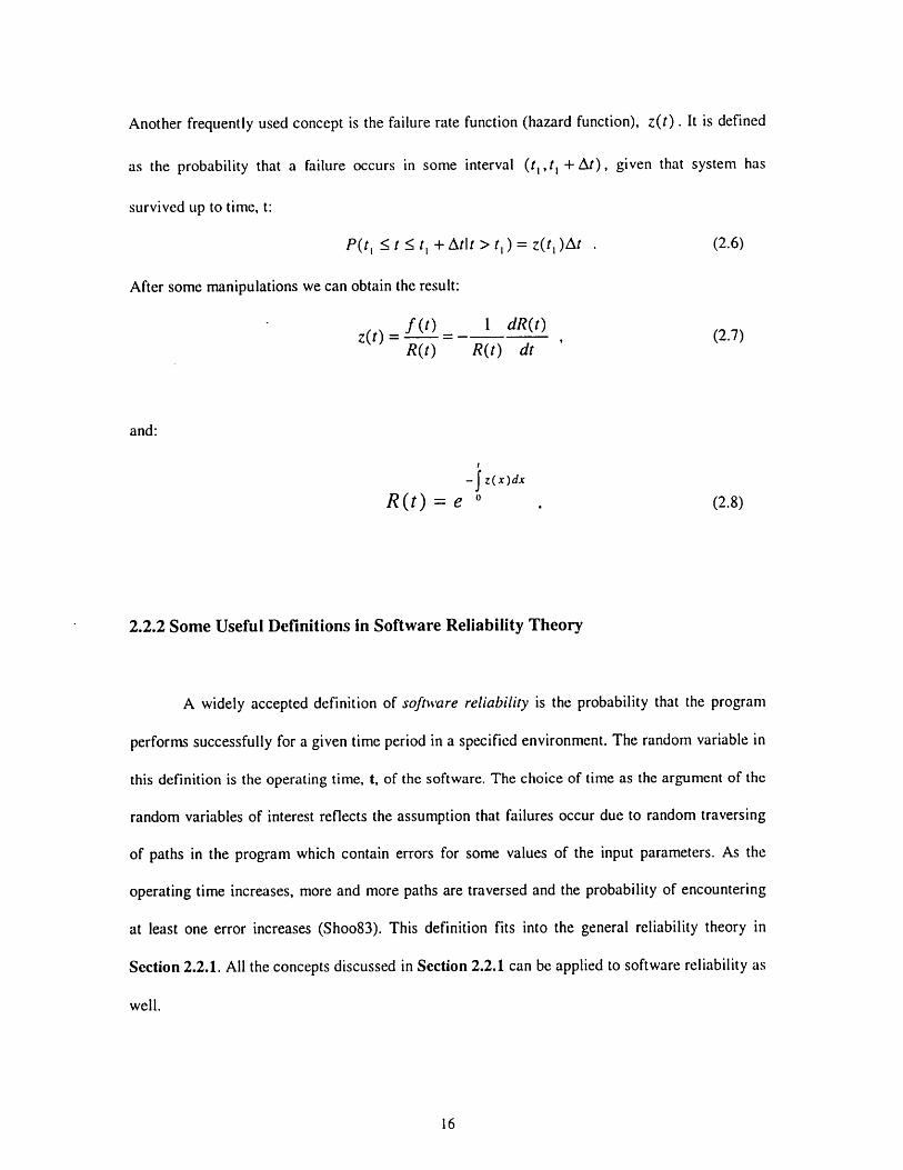
Another frequently used concept is the failure rate function (hazard function), z(t). It is defined

as the probability that a failure occurs in some interval (t,,t, t + At), given that system has

survived up to time, t:

P(t < t 5 t, + Atlt > t) = z(t )At . (2.6)

After some manipulations we can obtain the result:

f(t) 1 dR(t)

R(t) R(t) dt

and:

- z(x)dx

R(t) = e 0 (2.8)

2.2.2 Some Useful Definitions in Software Reliability Theory

A widely accepted definition of software reliability is the probability that the program

performs successfully for a given time period in a specified environment. The random variable in

this definition is the operating time, t, of the software. The choice of time as the argument of the

random variables of interest reflects the assumption that failures occur due to random traversing

of paths in the program which contain errors for some values of the input parameters. As the

operating time increases, more and more paths are traversed and the probability of encountering

at least one error increases (Shoo83). This definition fits into the general reliability theory in

Section 2.2.1. All the concepts discussed in Section 2.2.1 can be applied to software reliability as

well.

A failure is a departure of the external results of program operation from program

requirements on a run. A fault is a defective, missing, or extra instruction or set of related

instructions that is the cause of one or more actual or potential failure types (Musa87). In this

thesis another term error is often used interchangeably with the term fault.

An operational profile is a frequency distribution of input data that represents the typical

usage of the program. An oracle is any means that provides sufficient information about the

(correct) expected behavior of a program that it is possible to determine whether the software

produced the correct output corresponding to a set of input data (Beiz90).

2.3 Software Reliability Growth Models

Software reliability growth models are time-based reliability models. They are so called

because they try to predict the software's reliability evolution in the future. Software reliability

growth models take failure data from a period when faults are being detected and fixed, during

testing or operational use, and use this information to estimate the reliability of the program under

study and predict how this reliability will change in the future.

Usually, a software growth model contains three stages. First, the model structure is

selected according to some preliminary general assumption or specific hypothesis concerning the

software characteristics and the testing environment. Second, the free parameters in the model are

estimated by fitting the data from testing to the model. Finally, a rule is deduced for the fitted

model to be used for predictive purposes (Goos88).

Software reliability growth models can be grouped into two categories: Time Between

Failure Models and Failure Count Models.

2.3.1 Time Between Failure Models

In this class of models the variable under study is the time between failures. The models

are based upon statistical characterization of the time intervals between successive observed

failures. Let a random variable T denote the time between the (i-1)st and the ith failures. The

most common approach is to assume that T follows a known distribution, whose parameters

depend upon the number of faults remaining in the program after the (i-l)st failure. The

parameters are determined from the observed values of times between failures in the testing

phase. The fitted model can then be used to estimate the software reliability, mean time to failure,

etc. (Goel85)

One of the earliest and probably the most widely used model in this class is the

JelinskilMoranda (JM) De-eutrophication Model (Jeli72, Goos88). The JM model assumes that

t,t2,...are independent random variables with exponential probability density functions (ti

denotes the time between the (i-1)st and ith failures), where:

P(tilz(ti)) = z(t,)e-" ",ti > 0 , (2.9)

where z(t, ) is the failure rate at time, t1 :

z(t,)= [N-(i- 1)] , (2.10)

where is a proportional constant (a model parameter),

N is the total number of faults originally in the program (a model parameter).

The rationale for the model is as follows: The model assumes that the initial fault content

in the software is N before testing, each fault is independent of the others and is equally likely to

cause a failure during testing. During each of the interval between the (i-I)st and ith failures, a

fault is detected and removed with certainty and no new faults are introduced during the

debugging process (i.e., perfect debugging). The failure rate at any time is assumed to be

proportional to the current fault content, N - (i - 1), in the program.

The model parameters, N and , are estimated by maximum likelihood method.

Predictions are made by the "plug-in" rule: substitution of the maximum likelihood estimates,

N and 4, into the appropriate model expressions. For example, when t, ,t 2 ,..t 1 are the observed

data, the predicted (current) reliability is:

i (t) = e- (2.11)

where Ri (t) is an estimate of R, (t) = P(t < t).

The most serious criticism of this model is that it assumes perfect debugging and that all

faults contribute the same amount to the overall failure rate. It is argued by Littlewood (Litt81)

that the different frequencies of execution of different portions of code will in themselves lead to

different rates of fault occurrence, all other factors being equal.

Many other models in this class are extensions of the JM model with some modifications.

The Schick/Wolverton model (Schi78) is based upon the same assumptions as that of the JM

model except that the failure rate function is assumed to be proportional to the current fault

content of the program as well as to the time elapsed since the last failure:

z(t,) = [N -(i- 1)]t, . (2.12)

The model implies a linearly increasing time interval between failures, which is difficult to

justify.

Another extension of the JM model is the Goel/Okumoto imperfect debugging model

(Goel78). In this model, the number of faults in the system at time t, X(t), is treated as being

governed by a Markov process where the software can change its failure population state

randomly. In this process these transition probabilities are governed by the probability of

imperfect debugging. Times between the transitions of X(t) are taken to be exponentially

distributed with rates dependent upon the current fault content of the system. The failure rate

function during the interval between the (i-I)st and the ith failures is given by the relationship:

z(t,) = [N - p(i-1)] , (2.13)

where p is the probability of imperfect debugging,

A is the failure rate per fault.

The Littlewood/Verrall Bayesian Model (Litt73) takes a different approach from the JM

model. In this model, the times between failures are assumed to follow an exponential distribution

(Eq. (2.9)), which is the same as that of the JM model. However, the parameter of this

distribution, z(t, ), is treated as a random variable obeying a gamma distribution:

f (z(t,)Ia, y(i)) = (2.14)Fa

where a and T(i) are model parameters.

2.3.2 Failure Count Models

In this class of models the variable under study is the number of failures seen or faults

detected during given testing intervals. The time intervals may be a fixed priori, and the number

of failures in each interval is treated as a random variable. Most of the models in this class

assume that faults in the program are independent so that the failures have a Poisson distribution,

whose parameters take different forms for different models.

One of the earliest and simplest Poisson model is the Goel/Okumoto Nonhomogenous

Poisson Process (NHPP) Model (Goel79). The model assumes that software is subject to failures

at random times caused by faults present in the system. Let N(t) denote the cumulative number

of failures observed by time, t. The model treats N(t) as a nonhomogeneous Poisson process,

i.e., as a Poisson process with a time dependent failure rate:

(m(t))'P(N(t) = y) = e- ,y = 0,1,2,.. , (2.15)

y!

where m(t) is the mean value function, it gives the expected number of failures observed by time,

t, as:

m(t) = a(l - e -b ) . (2.16)

The failure rate is given by the relationship:

z(t) =- m'(t) = abe -b ' . (2.17)

The parameter a represents the expected number of failures eventually to be observed. The

parameter b can be interpreted as the occurrence rate of an individual fault and is a constant of

proportionality relating the failure rate to the expected number of faults remaining in the program.

The model is similar to the JM model in assuming a direct proportionality between the

failure rate and the number of remaining faults, but differs in modeling this proportionality

continuously, rather than by discrete steps when faults are removed. The model permits imperfect

debugging and the introduction of new faults during debugging, however, the interpretation of b

will be different in such cases.

The mean value function, m(t), in the Goel/Okumoto Nonhomogenous Poisson Process

Model is exponential on the time, t. Using a function, m(t), of this type assumes that software

quality continues to improve as testing progresses, and results in a monotonically decreasing

failure rate vs. time. Some other NHPP models use m(t) functions of different forms in order to

capture different realism in software testing.

In practice, it is observed that in many testing situations, the failure rate first increases

and then decreases. In order to model this behavior, Goel (Goel82) proposed a generalization of

the Goel/Okumoto Nonhomogenous Poisson Process Model. The model uses a mean value

function of the form:

m(t) = a(1- e- b' e ) , (2.18)

where a has the same meaning as that in the Goel/Okumoto NHPP model,

b. c are constants that reflect the quality of testing.

The failure rate function, z(t), is given by the relationship:

z(t) = m'(t) = abce-btc c-t . (2.19)

In practice, there is a delay between the fault detection and the fault removal. The testing

process in this case consists of two phases: fault detection and fault isolation/removal. S-shaped

NHPP. models are proposed to capture this realism (Ohba84, Gokh96). The mean value function,

m(t), is given by the relationship:

m(t) = a(1- (1+ bt)e -b') , (2.20)

where a,b have the same meanings as that in the Goel/Okumoto NHPP model.

The failure rate is given by the relationship:

z(t) - (t)t) = b'te -bt . (2.21)

Some other widely referenced models in this class include the Shooman Model (Shoo72),

the Musa Model (Musa71), the Generalized Poisson Model (Angus80), etc. During recent years

many models have been developed to model imperfect debugging and the introduction of new

errors during the debugging process. Examples include a Poisson type model (Bust94) and a

hyper-geometric distribution model (Hou95). These models are also based upon Poisson process

with new random variables introduced to model imperfect debugging. Complicated mathematics

is involved in these newly developed models and their details are omitted here.

2.3.3 Advantages and Limitations of Software Reliability Growth Models

Software reliability growth models have a long development history, which can be traced

up to the 1970's. Until now several growth models have been developed. Many of them have

been extensively studied, and have had real applications for various types of software in many

fields. By choosing the appropriate form of the model, many typical behaviors of the software

during the testing phase (e.g., the first increasing then decreasing failure rate) can be modeled.

Many practical concerns during the software testing (e.g., imperfect debugging) can be

incorporated into the models. Only testing data are required for the application of the growth

models, which makes them easy to implement and applicable to essentially all types of software,

ranging from a small module to a complex flight control system consisting of millions of lines of

code. The automation of the application of the growth models is relatively easy. Many automated

tools have been developed to facilitate the applications of the growth models and the comparison

of their results (Li95, Vall194, Vall195). For software without a very high reliability requirement,

satisfactory results can often be obtained if the appropriate growth model is used.

Despite of all these advantages, the growth models also have many limitations. First,

most of the models are based upon the assumption that all the faults in the program contribute

equally to the unreliability of the software, which typically is not realistic because the occurrence

frequencies of different types of faults may vary significantly. Secondly, the growth models

assume a typical operational profile of the software is available and base their testing upon such a

profile. If there are big errors or changes in the operational profile, the models may not produce

good results. Redoing the testing based upon the new operational profile may even be necessary.

Much research has been done to analyze the sensitivity of the model predictions to errors in the

operational profile (Chen94A, Cres96). No conclusive remarks can be made, though, due to the

limited set of case studies performed and discrepancies seen in the results. Finally, the predictions

of the growth models are typically not very accurate. The uncertainties associated with the growth

model estimations are high and there is no effective mechanism to assess the uncertainties. The

difficulty in validating the growth models makes them not well suited for applications to software

with a very high reliability requirement.

As a summary, the growth models treat the software as a black box and do not take the

structures of the target software into consideration. The overly simplified nature of the models

prevents the models from producing reliable estimations. Although many types of growth models

with different assumptions have been developed aiming to capture different characteristics of the

target software and the testing process, experiments have shown that the model whose

assumptions appear to best match these characteristics of the target software and the testing

process is not guaranteed to be the most appropriate model for use (Abde86, Niko95).

Experimental application of different models "..has shown that there is commonly great

disagreement in predictions, while none of them has been shown to be more trustworthy than

others in terms of predictive quality in all applications..." (Lu93). It is not a surprise to see that

application of reliability growth models to safety critical software, e.g., space shuttle applications,

failed to produce satisfactory results due to high uncertainties in their estimation (Dunn86,

Schn92).

2.4 Fault Seeding Models

The basic approach in this class of models is to "seed" a known number of faults in the

program, which is assumed to contain an unknown number of indigenous faults. The program is

then tested and the exposed number of seeded and indigenous faults is recorded. From the

recorded data, an estimate of the fault content of the program prior to seeding can be obtained and

used to estimate the software reliability.

The most popular fault seeding model is the Mill's Hypergeometric Model (Mill72). The

model randomly seeds a number of faults in the target program. The program is then tested for a

certain amount of time. The number of indigenous faults can be estimated from the number of

seeded and indigenous faults uncovered by the testing by using a hypergeometric distribution.

Some other models in this class include the Lipow Model (Lipow72), and the Basin Model

(Basin74).

The models in this class are economical and easy to implement. However, they are based

upon implicit assumptions that the indigenous faults are independent of one another, and that all

of the seeded and indigenous faults are detected with equal probability. The latter assumption is

so unrealistic that the models typically do not produce satisfactory results. Another serious

limitation of the seeding models is that there is no way to obtain the failure rate function. The

seeding models can only work as error count models. During recent years studies on the seeding

models have ceased. Although seeding is still an active technique in other applications (e.g., the

validation of reliability models), seeding models are rarely applied.

2.5 Input Domain-based Reliability Models

Before we discuss input domain-based reliability models, it is necessary to introduce

some related terms. The input domain of a given program is the set of all relevant inputs to the

program. The input subdomain is a subset of the input domain. A partition is a division of the

input domain into disjoint subdomains. An input subdomain is homogeneous if either all of its

members cause the program to succeed or all cause it to fail. Thus, any member in a

homogeneous subdomain is a good representation of the entire subdomain. A path domain is the

subdomain corresponding to a given path in a program, i.e., all the inputs in the subdomain cause

the same path to be traversed.

The basic approach taken by input domain-based models is to sample a set of test cases

from the input domain according to an input distribution (i.e., the operational profile), which is

representative of the operational usage of the program. An estimate of the program reliability is

obtained from the failures observed during the execution of the test cases. Since the input

distribution is very difficult to obtain, the input domain is often divided into subdomains and test

cases are generated randomly in each subdomain based upon a uniform distribution. Based upon

different ways to divide the input domain, the models in this class can be grouped into two

categories: random testing, and subdomain/partition testing.

2.5.1 Random Testing

Random testing method randomly and uniformly selects test cases from the entire input

domain. An earliest model in this category is the Nelson Model (Nels78). It is then extensively

studied by many other authors, and its performance is compared to the other testing strategies

(e.g., subdomain testing and partition testing) (Duran84, Chen94B, Chen96). For a program P,

denote its input domain as D and the size of D as d (>0). Let m (0 m < d) denote the number

of failure-causing inputs (i.e., the elements of D which produce incorrect outputs) in D. The

failure rate of the program, 0, is defined as:

m0 = -- (2.22)

d

Let n denote the total number of inputs selected for testing. Let n, denote the number of failures

observed during the execution of the in inputs. In other words, n, denotes the number of inputs

that resulted in execution failures. Then an estimate of 0 can be obtained by the relationship:

n9= n, . (2.23)

n

If the program is executed for a long period of time using a given input distribution, then the

actual failure rate of the program will converge to the probability that the program will fail to

execute correctly on an input case chosen from the particular input distribution. An unbiased

estimate of the software reliability per execution, R, can be obtained by the relationship:

R=1-0=1L n,. (2.24)n

An estimate of the software reliability on K successive executions is given by the relationship:

R=(1- )K . (2.25)

A useful quantity for assessing the effectiveness of random testing and comparing its

performance to that of other testing methods is P,, the probability of finding at least one error in

n tests.

P, = 1 - (1 - 8)" . (2.26)

Another significant quantity is 8', the (1- a) upper confidence limit on 0. 0" is the largest

value of 0 such that:

(n)o'(1-6)"-' >a. (2.27)

If the number of errors found n, = 0, then:

0 = 1-a " . (2.28)

In this case 0" decreases as the total number of tests n increases. 06 --4 0 as n -4 o.

Eq. (2.27) and Eq. (2.28) provide an effective mechanism to assess the uncertainty associated

with the model estimate.

2.5.2 Subdomain/Partition Testing

Both subdomain testing and partition testing divide the input domain into subdomains,

one or more test cases from each subdomain are selected to test the program. The term

subdomain testing is used for the general case when the subdomains may or may not be disjoint.

The term partition testing is used for the special case when all subdomains are disjoint (Chen96).

In this section we will focus on partition testing because it is more extensively studied. However,

most of the results can also be applied to subdomain testing.

Partition testing refers to any test data generation method that partitions the input domain

and forces at least one test case to be selected from each subdomain. Suppose the input domain D

is partitioned into k subdomains, which are denoted by D,, where i=1,2,..k. Each subdomain D,

has size di, contains m, (0 < mi < d, ) failure-causing inputs, and has failure rate:

0, = m . (2.29)di

Let p, denote the probability that a randomly selected input comes from the subdomain D,. The

failure rate of the entire program is given by the relationship:

k

0 = p1 0 . (2.30)

Use n, (> 1) to denote the number of test cases selected from the subdomain D i.Use n,, to

denote the number of test cases select from the subdomain Di which result in program failures.

All the random selections are also assumed to be independent, with replacement, and based upon

a uniform distribution. This means that when a test case is selected from D,, the probability that

it is a failure-causing input will be exactly 08,. An estimate of the overall failure rate of the

program, 0, can be obtained using Eq. (2.23). Another estimate of 0 is given by Lipow

(Lipow75):

k k

0 =1 P P =I Pi (n,,) (2.31)i=1 1=1 n,

Then Eq. (2.24), (2.25) can be used to estimate software reliability.

P,' the probability of finding at least one error in n tests is given by the relationship:

k

P,, = 1- (- 8,)", . (2.32)

The confidence limit of the estimate of partition testing strategies takes more complex form than

Eq. (2.27). It varies for different strategies.

Research has been conducted to compare the performance of partition testing with that of

random testing (Duran84, Weyu91, Chen94B). Results show that using the same number of test

cases, partition testing in general is not more cost-effective than random testing unless some

conditions are meet, such as the proportional rule produced by Chen (Chen94B). A special case

occurs when the subdomains are homogeneous. In this case only one test case is needed for each

subdomain. The total number of test cases required by partition testing will be greatly reduced

and become much less than that required by random testing. Nevertheless, a truly homogeneous

subdomain is very difficult to obtain in practice. Most of the partition testing strategies developed

by now attempt to produce more or less homogeneous subdomains (i.e., the inputs in the

subdomain share some similarities in error revealing capability) with manageable effort.

Examples include the data flow testing criteria, a family of testing strategies developed by Rapps

and Weyuker (Rapps82, Rapps85). The strategies require the exercising of path segments

determined by combinations of variable definitions and variable uses. Popular code coverage

strategies can be considered to be partition testing strategies. The statement/branch/path testing

requires that sufficient test cases be selected so that every statement/branch/path in the program is

executed at least once. Note that only path testing divides the input domain into disjoint

subdomains. Mutation testing (DeMi78, Offu96) can also be viewed as a partition strategy.

2.5.3 Advantages and Limitations of Input Domain-based Reliability Models

Input domain-based models have many advantages over the reliability growth models.

First, input domain-based models do not depend upon the unrealistic assumption that that all the

faults in the program contribute equally to the unreliability of the software. By selecting the test

cases based upon a given input distribution, input domain-based models implicitly weigh the

contribution of a fault to the software unreliability by p , the probability that a randomly selected

input belongs to an equivalent class which exercises the fault (i.e., the occurrence rate of the

fault). Secondly, by choosing appropriate testing strategies (e.g., the code coverage strategies),

more information of the target program (e.g., the control structure and the data usage) can be

incorporated into the models. The white box treatment of the program can be expected to be

superior to the black box treatment by reliability growth models and able to generate better

results. Thirdly, input domain-based models provide an effective mechanism to assess the

uncertainties in the reliability estimation (e.g., Eqs. (2.27) and (2.28) for random testing).

Assuming detecting no errors, which is typical in the later testing phase of safety critical

software, the uncertainty associated with the reliability estimation decreases as the total number

of test cases n increases. Theoretically it is possible to obtain any accuracy in reliability

estimation after performing sufficiently large number of test cases. Thus input domain-based

models are particularly suited for applications to safety critical software, in which high accuracy

and high certainty is required for reliability estimation. Finally, input domain-based models can

easily accommodate changes in the operational profile. Input domain-based models randomly

select test cases from each subdomain using a uniform distribution. Changes in the operational

profile only have effect on the estimation of 0 through the changes in the p, 's (Eq. (2.31)). Only

the p, 's need to be recomputed using the modified operational profile, test cases need not to be

regenerated.

Input domain-based models also have several limitations. First, an underlying

assumption made by both random testing and partition testing is that no fault is removed

and the software reliability remains unchanged during the testing process. In practice

faults are identified and removed from the program during testing and the software

reliability is expected to improve during the testing process. Input domain-based models

are too conservative in such sense. Secondly, the application of input domain-based

models is much more complex than that of growth models. In order to produce more or

less homogeneous subdomains, structural information of the target program is often

required. Typically complex testing strategies have to be applied to control the partition

process, the generation of test cases, and the testing process. Automation of the modeling

is often necessary for relatively small programs (compared with what can be handled by

growth models), while very few automated tools of this kind are available now. Finally,

input domain-based models randomly select test cases form each subdomain using a

uniform distribution rather than using the actual input distribution, which introduces

errors into the reliability estimation. One exception is that if the subdomains are truly (or

very close to) homogeneous, either all inputs in the same subdomain cause the program

to fail or none of the inputs causes a failure (i.e., 0, in Eq. (2.31) is either one or zero).

The input distribution inside the subdomain has no effect on the reliability estimation.

Only the pi of the subdomain needs to be estimated with high certainty.

In recent years input domain-based models are receiving more and more interest

as a promising technique for reliability estimation for safety critical software, especially

after the unsuccessful experience of applications of reliability growth models (Dunn86,

Schn92). Nevertheless, input domain-based models are still at the beginning of their

development stage. Many difficulties have to be overcome before their wide and success

applications. Much work needs to be done in this area.

Chapter 3

The Integrated Methodology

This chapter formulates an integrated methodology for reliability estimation of safety

critical software. The methodology is built upon an input domain-based reliability model using a

path testing (partition) strategy. Section 3.1 introduces the control flowgraph and some other

related concepts that are used extensively in the thesis. Section 3.2 presents some fundamental

definitions and equations that comprise the theoretical foundation of the methodology. Elements

of the methodology are discussed in Section 3.3 through Section 3.6. A summary of the

advantages and limitations of the methodology is given in Section 3.7.

3.1 The Control Flowgraph

The proposed integrated methodology is based upon the concept of structured path

testing. Before we introduce the definition of the path, it is first necessary to introduce the control

flowgraph concept. In general, the control flowgraph is a graphical representation of the control

structure of a program.

3.1.1 Elements of the Control Flowgraph

The control structure of a program is composed of three different types of elements,

namely, process block, decision, and junction. The process block is composed of a group of

statements that must be executed in a sequential order from the entrance to the exit. The length of

the process block can vary from one to hundreds of statements. The decision is a section of code

where control flow can diverge into different paths. The standard decision construct is the

if.then..else statement which relies upon the value of the predicate, a Boolean function of certain

variables, in order to decide which path will be executed. The junction is a section of code where

control flows can merge together. For example, when the separate true and false paths end after

an if.then statement, the flow can merge together to form a junction. All computer programs can

be broken down into some combination of these three elements.

The control flowgraph is composed of two types of components: circles and lines (with

arrows). A circle is called a node and a line is called a link. A node with only one link entering

and only one link exiting is a process node, which is used to represent the process block structure

(Fig. 3.1).

Figure 3.1 A process node

A node with more than one link exiting is a decision node, which is used to represent a decision

structure (Fig. 3.2).

Figure 3.2 A decision node

A node with more than one link entering is a junction node, which is used to represent a junction

structure (Fig. 3.3).

In some cases statements can be both decisions and junctions, such as loop control

statements. The corresponding nodes have more than one link entering and more than one link

exiting.

From the above all control structures can be expressed using the control flowgraph.

Figure 3.3 A junction node

3.1.2 An Illustrative Example

In this section an example program will be analyzed and its control flowgraph

constructed in order to facilitate the understanding of the control flowgraph concept. The example

program used here is taken from Lunglhofer's report (Lung96). The readers can refer to Section

2.2.1.2 in Lunglhofer's report for the original statements. The language used is a pseudo

programming language based upon that developed by Rapps and Weyuker in 1985 (Rapps85).

The purpose of using this language is to break down any language barriers other high level

Figure 3.4 The pseudo programming language

(Duplicated from Fig. 2-4 in Lung96)

Elementary programminglanguage for exemplary use.

* Begin statement: Begin* Input statement: Read x,. . . ,x n

(x , .. . , xn ) are variables.* Assignment statement: y <= f(xl, . . , xn )

(y, X 1, .. , xn are variables) and f in a function.* Output Statement: Print zI .... , zn

(z, . . . , zn )are either littorals or variables.* Unconditional Transfer Statement: Goto im

m is a label.* Conditional Statement: If p(xl , ... , xn) Then

statements executed if predicate p is trueElse

statements executed if predicate p is falseEnd If

p is a predicate on the variables (x 1, .. , xn). ConditionalStatements can be nested.

* End Statement: End

I

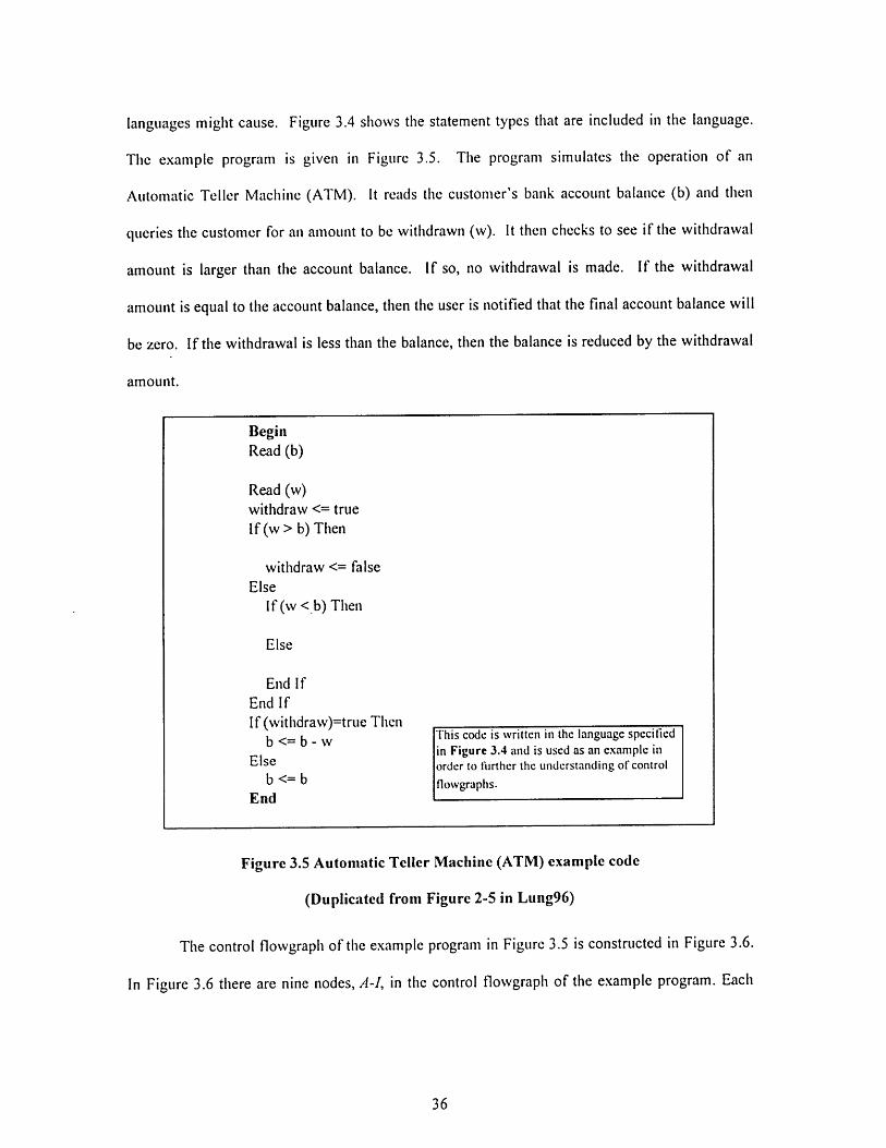
languages might cause. Figure 3.4 shows the statement types that are included in the language.

The example program is given in Figure 3.5. The program simulates the operation of an

Automatic Teller Machine (ATM). It reads the customer's bank account balance (b) and then

queries the customer for an amount to be withdrawn (w). It then checks to see if the withdrawal

amount is larger than the account balance. If so, no withdrawal is made. If the withdrawal

amount is equal to the account balance, then the user is notified that the final account balance will

be zero. If the withdrawal is less than the balance, then the balance is reduced by the withdrawal

amount.

BeginRead (b)

Read (w)withdraw <= trueIf (w > b) Then

withdraw <= falseElse

If(w < b) Then

Else

End IfEnd IfIf (withdraw)=true Thenb <= b - w

Elseb <= b

End

This code is written in the language specifiedin Figure 3.4 and is used as an example inorder to fiurther the understanding of control

flowgraphs.

Figure 3.5 Automatic Teller Machine (ATM) example code

(Duplicated from Figure 2-5 in Lung96)

The control flowgraph of the example program in Figure 3.5 is constructed in Figure 3.6.

In Figure 3.6 there are nine nodes, A-I, in the control flowgraph of the example program. Each

consists of a single statement or a block of statements. In Figure 3.6, B, D, E, G andH are process

nodes; A, C and F are decision nodes; F and I are junction nodes.

ATM Code Control Flowgraph Breakdown

Read (b) I Statements APrint ("Enter amount to withdraw.")Read (w)withdraw <= trueIf (w > b) Then

Print ("Amount to withdraw exceeds balance.") Bwithdraw <= false

Else

If(w < b) Then IC

Print ("lhank You.") D

Else

Print ("Thank You, Your final balance will be $0.00") IE

End IfEnd If

If (withdraw)=true Then F

b <= b - w G

Else

<= b H

lEnd II

Figure 3.6 ATM example code and its flowgraph


Flowgraph

3.1.3 Some Useful Terms

Using the control flowgraph of the example program in Figure 3.6, we can introduce

some terms that are used extensively in this thesis (Rapps85, Lung96). The links in the control

flowgraph are also known as edges. An edge from node j to node k is given the notation (", k).

Node j is called a predecessor of node k, and node k a successor of node j. The first node of a

program is called the start node and has no predecessors, e.g., node A in Fig. 3.6. The last node is

called the exit node and has no successors, e.g., node I in Fig. 3.6. A path orflow path is a finite

sequence of nodes connected by edges. A path is designated by a sequence of nodes. For instance,

a path in Fig. 3.6 is Path I=(A+B+F+G+I). A path is a complete path if its first node is the start

node and its last node is the exit node. A path is a loop free path if none of its nodes is repeated in

the sequence. If any node in a path is repeated, the path contains a looping structure. Following

these definitions Path 1=(A+B+F+G+I) is both a complete path and a loop free path. A path is a

feasible path if some inputs exist that will cause the path to be traversed during program

execution. For instance, a feasible path in Fig. 3.6 is Path 2=(A+B+F+H+I), which will be

executed if we assign input variables to be w=200, b=100. A path is an infeasible path if no input

exists that will cause the path to be traversed during program execution. For instance, Path

I=(A+B+F+G+I) is infeasible. Whenever block B is executed, the variable "withdraw" will be

set to false, and block G will not be executed thereafter.

3.2 The Underlying Software Reliability Model

For a given software, use N,,,,,, to denote the total number of paths in the program. Use

N,,,,, to denote the total number of paths identified in the software through structural analysis.

Use N,,,,,,, to denote the number of paths that are tested in the testing phase. Use N,,,,,, i to

denotes the number of paths that are identified but not tested. Clearly we have:

Ni et, = Nl,,,,I + N,,,,,,,t * (3.1)

For any path, i, in the software, use D, to denote the corresponding path subdomain.

Use 0, to denote the probability of failure upon a single traverse of the path i. From Eq. (2.29) in

Section 2.5.2:

sO = mI, (3.2)di

where m, (0 m, < d,) is the number of failure-causing inputs in D,,

d, is the total number of inputs in D,.

Use p, to denote the probability that the path, i, will be traversed in a single program execution,

averaged over the program lifetime. It is equivalent to the p, defined in Section 2.5.2. From Eq.

(2.30) in Section 2.5.2, the failure rate of the entire program is:

0= Zp,O, . (3.3)

An estimate of the failure rate, 0, is given by:

0= EA, . (3.4)

Use P to denote the probability that an identified path will be traversed in a single program

execution.

P= p, . (3.5)i-1I

P is equal to unity if all the paths in the program are identified. In reality, it is not always possible

to identify all the paths in a program, especially when the program contains looping structures. In

such cases P is less than unity. Use Qr. to denote the unreliability contribution of the N,,ted,

tested paths. Use Q, to denote the unreliability contribution of the N,,e,,,,, untested paths:

QT = p, 0, (3.6)

Qu = Ep,, (3.7)i. N,,a, + I

Another estimate of the failure rate, 0, can be obtained as:

I N,," 0QQ,) I (3.8)P = - -- ( + 1)P i.i P

An estimate of software reliability per execution is given by the relationship:

R = 1 - . (3.9)

An estimate of software reliability on K successive executions is given by the relationship:

R= (1-)K . (3.10)

The methodology is essentially a partition testing method using a path testing strategy.

The input domain D is partitioned into path subdomains, D, 's, in such a way that, all the inputs

in a subdomain lead to the execution of the same path, i, in the software. The product, p,O,,

corresponds to the unreliability contribution of the path subdomain, D,. Since the inputs in a path

subdomain lead to the execution of the same path in the software, it is very likely that they will

reveal the same errors in the software. In other words, the path subdomain can be expected to be

more or less homogeneous. Based upon this partition strategy, the methodology we proposed is

expected to produce better results than that of random testing.

Using the above definitions, the estimation of the software reliability is reduced to the

estimation of pi and 0i for each path in the software. p, is closely related to the operational

profile of the software. The estimation of p, is discussed in Section 3.4. 0B is closely related to

the fault content in the path. The estimation of 0, is discussed in Section 3.5. If both p, and 8,

can be estimated with high certainty, the quantitative value of the reliability of the software, R ,

can be obtained using the above equations with high certainty.

3.3 The Feasible Structured Path Testing Method

Since in the methodology the definition of the software reliability is based upon paths in

the software, the first step in the methodology is to identify all the possible paths in the software.

In reality, it is not always possible to identify all the paths in a software, especially when the

software contains looping structures. In such case, we wish to identify most of the paths in the

software in order to assure high accuracy in the reliability estimation. The testing method we

employed in this methodology for path identification is called the Feasible Structured Path

Testing (FSPT) method. The method is developed by Jon R. Lunglhofer (Lung96). It is chosen for

our use because it has several desirable features such as the ability to identify all the executable

paths in certain cases, not overly time consuming, and the ability to identify and remove

infeasible paths. Using this method, most (sometimes all) of the executable paths in a software

can be identified.

Although we chose the Feasible Structured Path Testing (FSPT) method as the testing

method for our methodology, it needs not to be the only choice. Any other path testing method

that is able to identify some of the paths in the program is also applicable to our methodology.

After the paths are identified, all the other elements of the methodology can be applied in the

same manner independent of the testing method. Since the FSPT method is used in our case study

in Chapter 4, elements of the FSPT method will be presented in this section to help the readers

understand the process. Interested readers can find more details of the testing method in

Lunglhofer's report (Lung96).

3.3.1 Method Overview

The feasible structured path testing method is based upon the concept of structured path

testing method. Structured path testing method attempts to test every path in the software, i.e., to

achieve path coverage. It differs from the complete path testing in that it limits the number of

loop iterations to a value, k. If a looping structure exists in a section of code, the loop is only

executed k times through at most. This strategy sacrifices completeness, however, it produces a

finite and manageable set of paths, which is necessary for the software analysis and testing to be

practical. The feasible structured path testing method adds a step to the structured path testing

method to determine and eliminate infeasible paths in the control flowgraph, which greatly

simplifies the control flowgraph and reduces the number of test cases required.

3.3.2 Method Details

"The feasible structured path testing method consists of a five step formal process. The

goal of the process is to take a program, and through analysis to systematically produce test cases,

which achieve structured path testing coverage involving no infeasible test cases." (Lung96) The

five steps are discuLsed in detail in this section, some are quoted from Lunglhofer's report, and

some are modified and reformulated in this thesis.

Step 1: The first step of the Feasible Structured Path Testing (FSPT) method examines

the program being analyzed and constructs the program's control flowgraph. The construction

process has been illustrated in Section 3.1.3. In the case that looping structures are present in the

code, one expands the flowgraph to include at most k iterations of any looping structure. An

example of the expansion (k=2) is given in Figure 3.7. There are several factors in selecting the

appropriate value of k. When k is small, the number of paths that are included in the control

flowgraph is small, and the number of test cases required is small. Ask increases, more and more

paths will be included in the control flowgraph. The effort needed in analyzing and testing the

program will increase, while the probability of detecting more errors will also increase. A

complete test occurs when k reaches infinity or the maximum value of loop iterations specified in

the program. Based upon the requirement of the analysis and the time and resources available,

the analyzer can choose the value of k that is best suited for his own application.

Expanding a flowgraph to show k iterations

A

General flowgraph

BA

B

C

Figure 3.7a

Expandedflowgraph forcase k=2.

a

b

Figure 3.7b

The flowgraph in Figure 3.7a is expanded into two iterations of theloop represented in the path A+B+A in Figure 3.7b. In the caseabove the value of k is two.

Figure 3.7 Flowgraph expanded to k iterations


The first step assumes that no horrible loops exist in the code. Horrible loops are

described by Beizer as ". . . code that jumps into and out of loops, intersecting loops, hidden

loops, and cross-connected loops .. ." (Beiz90). Figure 3.8 shows an example of horrible loops.

Horrible loops in a program are troublesome in expanding the looping structures and generating

the control flowgraph. They make the program difficult to understand and complicate the analysis

and debugging of the program. They are often resulted from poor programming experience and

should be avoided by all means in high quality software. The FSPT assumes that the program

contains no horrible loops.

Anexampleof ahorrible

loopstructure.

Figure 3.8 Horrible Loops


Step 2: The second step identifies the transitional variables in the program. The

transitional variables will then be used in the third step. The next a few paragraphs are quoted

from Lunglhofer's report (Lung96) to show the meaning of the transitional variables and the way

to identify them.

"2.1 The second step involves an examination of the data flow of the program, and results

in a list of variable transitions. These transitions relate the input variables to the output variables.

The first step of the process is recognizing the input and output variables of the code. Any

variable or data object that attains its value from outside the piece of code being examined is

considered an input variable. Those variables which facilitate the ultimate use of the program are

known as output variables. To recognize the output variables, one must have some understanding

of the program's function. Output variables are produced in several ways. A function can be

performed and its products presented on an output device (e.g. a monitor), data can be stored in a

memory device (e.g. RAM) for later use, or in the case of testing a program module, variables can

attain values for use in other modules. Once the tester recognizes both input and output variables

of the code, the remainder of the second step can begin.

2.2 A list of every variable which directly affects the flow of data from the input to the output

variables is generated. This list contains the transitional variables. For a variable to be included

in the list of transitional variables, it must meet one of two requirements. The variable can

directly attain its value as a function of an input variable, or of another transitional variable.

Also, other variables are designated transitional variables by directly affecting the value of the

output variables, or by affecting the values of other transitional variables which affect the output

variables. Recall from the exemplary language, detailed in Figure 2-4 (Figure 3.4 in this thesis),

the assignment statement: y <=f(xl,..... x,,) where (y, xl .... . , x,) are variables. In order for a

variable to be included in the transitional variable list, it must be created from an assignment

statement involving either input variables or other transitional variables already assigned to the

list. The relationship also works in reverse. If y is the output variable or another transitional

variable, then x1, . . . . x,, are added to the list of transitional variables. When all flow branches

have been examined including as many as k iterations of any looping structure, one should have a

complete list of every transitional variable leading from the input to the output variables. When

this list is complete, one can move on to the third step of the process." (Lung96)

Step 3 The third step further expands the control flowgraph obtained in step 1 with

respect to the transitional variables obtained in step 2. The next a few paragraphs are quoted

from Lunglhofer's report (Lung96) to show the expansion.

"3.2 Starting from the top node, one systematically examines the state of the

transitional variables that exist in each node. If a node contains a transitional variable that has not

reached the end of its development, the transitional variable affects other transitional variables or

the output variables at some point further down the execution path. It is necessary to expand the

flowgraph into a parallel structure reflecting each possible unique state of that transitional

variable. The number of states produced depends upon the number of possible paths reaching the

node in question. For instance, in Figure 3-2 (Figure 3.7 in this thesis), if at node C a transitional

variable x exists that affects the program's output variables, node C is expanded. If a unique

value of the variable x arises from each of the three paths leading into node C, node C expands

into three separate nodes and a new exit node is added." (Lung96)

Figure 3.9 shows an illustration of the expansion.

\ Figure 3.9bFigure 3.9a 3.

The flowgraph on the left is expanded at node C to

reflect the three unique states of the transitional variable

x which leads to the program output at node F.

Figure 3.9 Flowgraph expansion with respect to

transitional variables


Expanding a flowgraph to show unique

transitional variable states.

The expansion of the flowgraph in step 3 can also be performed in another equivalent, yet

more straightforward way. For each node in the flowgraph, if it has more than one, say, I1, links

entering, one expands the node into I seperate nodes and makes I copies of all the nodes below the

node (i.e., the successors of the node, the successors of the successors of the node..). This is a

naive way to achieve path coverage. More complex algorithms may be employed to reduce the

total number of paths needed for path coverage to improve efficiency. It is not a focus of our

work and is not discussed here.

Step 4 In Section 3.2.2 in Lunglhofer's report (Lung96), the fourth step in the FSPT

finds the value of the McCabe's metric (McCa76) of the flowgraph altered in step 3. "This value

is then used to determine the number of test cases needed to completely test the code. As

described in Section 2, a base test path is selected, and a set of linearly independent paths is

chosen from the code. These paths represent the complete set of the FSPT test cases." (Lung96)

After a closer look at the expanded flowgraph obtained after step 3 (e.g., Figure 3.9b), we can see

that after the expansion in step 3, the number of independent paths in the control flowgraph is

simply the total number of paths in the flowgraph. Thus the calculation of the McCabe's metric

and the identification of the independent paths is not necessary. From the expanded flowgraph

obtained after step 3 (e.g., Figure 3.9b), we can also see that the expanded flowgraph has such a

property that the path coverage is equivalent to the branch coverage. Finding all the paths in the

expanded flowgraph is equivalent to covering all the branches in the program. This is a big

advantage that can be obtained by performing step 3 because automation of the branch coverage

is much easier to achieve in practice than that of the path coverage. Thus the step 4 in the

modified FSPT is reduced to finding all the paths in the expanded flowgraph, or equivalently,

covering all the branches in the flowgraph.

Step 5: The fifth step in the FSPT determines the values of the input variables that cause

each test path to be executed. The step also determines which test paths are infeasible. These can

be done through predicate analysis.

3.3.3 Method Automation

Automation of the Feasible Structured Path Testing (FSPT) method requires automatic

generation of the control flowgraph, expansion of the flowgraph, and generation of the test cases.

Automatic generation of the control flowgraph for a given program is relatively easy. It is

incorporated in most symbolic execution tools (Clark76, Rama76, Kemm85, Coen90, Jasp94),

and many other Computer Aided Software Engineering (CASE) tools (Webb87, Heis93, Bhat94,

Harr95). The expansion of looping structures in the flowgraph to allow fork iterations is a simple

task and can be easily implemented. The expansion of the flowgraph with respect to the

transitional variables requires data flow analysis of the program, which is incorporated in most of

software reverse engineering tools (Fran85, Webb87, Heis93, Bhat94, Rich94, Lyu94, Harr95).

The most difficult step in automating the FPST method is the identification of infeasible paths

and the generation of test cases.

The most widely used method for path-driven test data generation (i.e., generation of test

data for a given path) is the symbolic execution technique. A common approach to symbolic

execution is to construct a control flowgraph of a given program. Each path in the flowgraph is

represented by a series of input variables, condition predicates and assignment statements. A set

of paths in the flowgraph are selected for testing, either by the user or by the symbolic executor

based upon certain criteria. Each of the selected paths is then traversed symbolically, i.e., each

input variable is given a symbol in place of an actual value, each assignment statement is

evaluated so that it is expressed in terms of symbolic values of input variables and constants. At

the end of the symbolic execution, the output variables of the path will be represented by

expressions in terms of symbolic values of input variables and constants, subjecting to certain

constraints. The constraints, often called the path conditions (PC), are provided by the set of

symbolic representations of each condition predicate along the path.

The feasibility of the path can be determined by checking the consistency of the

constraints. If there is any contradiction, the path is infeasible. This is often done by a theorem

prover embedded into the symbolic executor.

The generation of test case for the path reduces to finding a set of input variables that

make all the constraints satisfied. Then the outputs of the path execution can be obtained by

substituting the actual values of the input variables into the symbolic expressions of the output

variables. The feasible inputs are often found using linear programming (for linear constraints)

and nonlinear programming (for nonlinear constraints) technique. The technique attempts to

optimize an arbitrary objective function using the path constraints with the aim to find a feasible

solution satisfying all the constraints, making use of the fact that an optimal solution is also a

feasible solution. The technique has been extensively studied and many packages are available

which facilitate its implementation. Many existing symbolic executors employ this technique,

such as ASSET(Clar76), CASEGEN(Rama76), DISSECT(Howd77), Fortran Testbed (Henn83).

However, the complexity (both time and space) associated with its application is still very high

and it can not guarantee finding a feasible solution even if such a solution exists, especially when

nonlinear constraints are present.

Another method appearing in the literature is the trial-and-error method (Inam89). The

method randomly generates inputs and checks if the inputs satisfy all the constraints. Since the

efficiency of the method is problematic and no real applications have been found, the method is

not discussed in detail here.

The symbolic execution method has great difficulties in handling dynamic data

structures, array references, and modular calls. In order to overcome these difficulties, recently an

alternative approach of test data generation has been proposed by Korel (Korel90, Korel92,

Korel96). The approach ".. is based on actual execution of the program under test, function

minimization methods, and dynamic data flow analysis. Test data are developed for the program

using actual values of input variables. When the program is executed, the program execution flow

is monitored. If during program execution an undesirable execution flow is observed (e.g., the

"actual" path does not correspond to the selected control path) then function minimization search

algorithms are used to automatically locate the values of input variables for which the selected

path is traversed. In addition, dynamic data flow analysis is used to determine those input

variables responsible for the undesirable program behavior, leading to significant speeding up of

the search process." (Korel90) The approach is based upon actual execution of the target

program, thus having great advantages over the symbolic execution method in handling dynamic

data structures, array references, and modular calls. The effectiveness of test data generation can

be significantly improved. A limitation of the approach is that it has very limited ability to

detected path unfeasibility. A combination of the approach with the symbolic execution method is

suggested to overcome this difficulty (Korel90). Although the approach seems to be promising,

no real applications have been found in the literature.

Some other methods for automatic test case generation include the Genetic Algorithm

Approach (Hunt95, Rudn97, Mich97) which uses a combinatorial optimization technique; and the

Chaining Approach (Ferg95, Ferg96) which uses data dependence analysis. These methods are

not path-driven and can not be employed for our applications. Their details are omitted here.

As a summary, automatic identification of infeasible paths and generation of test cases

for given paths are very difficult to implement in practice. The tools available now have limited

capability on this aspect and can not always produce correct results. Due to limited time and

resources, we do not attempt to solve this problem, rather leave it for future research. Instead of

developing path computation and test case generation algorithms, the focus of this work is setting

up a framework for software reliability quantification.

3.4 The Estimation of p,

After a set of paths is identified using the testing method discussed in Section 3.3, the

estimation of p, for each of the paths can be done in two steps. First the operational profile of the

software has to be estimated. Then p, can be estimated based upon the operational profile. As we

will see in the following two sections, both steps are very difficult to implement in practice,

which makes the estimation of p, the most difficult element of the methodology.

3.4.1 The Estimation of the Operational Profile

The operational profile is essential to the estimation of p, and has to be obtained in some

way. The operational profile generally is not determined by the software itself but by some other

systems providing inputs to the software. A higher level of knowledge of the operational

environment of the software is required. The acquisition of the operational profile is very difficult

in practice. The software may have millions of input variables and the complexity in acquiring the

operational profile can be unmanageable. The software may have applications in a variety of

environments and the averaged operational profile is hard to obtain. The application environment

of the software may be highly dynamic and unpredictable and a "typical" operational profile does

not exist. All these factors contribute to difficulties in obtaining the operational profile in practice.

However, for nuclear control software, things are somewhat easier. Nuclear control software is

special purpose software and has a specific application environment, which is typically

predictable and not highly dynamic. During most of the software application lifetime the input

variables vary smoothly and over narrow ranges. For simple nuclear control software with

relatively few input variables, it is possible to accumulate enough knowledge to obtain an

estimate of the operational profile with certain accuracy. Due to limited time and resources we do

not go any further in handling this difficulty in the thesis and assume we can obtain the

operational profile in some way.

3.4.2 The Estimation of p, Based upon the Operational Profile

Even if the operational profile of the software can be obtained, it is still very difficult to

estimate p based upon the operational profile. There are two possible solutions, namely, the

direct integration method and the Monte Carlo method.

3.4.2.1 The Direct Integration Method

The operational profile can be expressed as a joint probability distribution

function,f(xl,x 2,..x,,), of the input variables x,,x 2 ,..x,,. The joint probability distribution

function, f(x, ,x,,..x,,), satisfies the normalization constraint:

fl(x 1,x,..x,,)dl...d,, = 1 , (3.11)

where D is the input domain.

p,, by definition, is the integration of the operational profile, f(xl,x,,..x,,), over the path

subdomain, D,, corresponding to the path, i:

P = , f(x,x,,..x,,)dxdx,..dx,, (3.12)

If the input variables are independent of one another, the equations are simplified to:

f(x 2,x,, ) = fx,) * '2 x,** f,, (x,,) , (3.13)

fi,(xj)dxj =1, j=l..n , (3.14)

p = f i (x )dx . (3.15)

The direct integration method thus consists of three steps: Obtain the operational profile

in the form of fJ(x,, x,,..x,,); identify the path subdomain, D,; then integrate

f'(x,,x 2 ,.x,) over the subdomain, D,.

Although mathematically elegant, the complexity associated with the method is so high

that the method is not feasible in practice. Firstly the operational profile may not be available in

the elegant form of f(x ,x,,..x,,) . In practice the operational profile is typically obtained by

consulting system users. It is often available in a partially integrated form, e.g., the probabilities

that the input variables have values in certain ranges [a,b]. Much effort is needed to convert the

operational profile into the appropriate form of f(xx, ,..x,, )

Secondly, the path subdomain corresponding to a particular path is very difficult to

obtain. As we have seen in Section 3.3.3, even finding a single input point in a path subdomain is

a very hard problem and can not be solved effectively by the currently available methods, e.g., the

symbolic execution method. Identifying the entire path subdomain is a much more difficult

problem than finding a single point in the path subdomain. It requires identification of all the

boundaries of the subdomain. In nuclear control software most of the predicates are linear (i.e.,

the predicates are linear Boolean functions of their variables). The boundaries of the

corresponding input subdomains are linear on their variables and the subdomains are generalized

polygons. No method was found in the literature survey to solve this problem even in this

simplified case. For nonlinear predicates the subdomains have much more complex shapes and

the difficulties in solving the problem increase even further.

Thirdly, the integration off over a path subdomain is a multidimensional integration and

is very computational intensive. From a search on the Guide to Available Mathematical Software

(GAMS) on the web, many mathematical packages are available now which contain subroutines

to evaluate a multidimensional integral numerically on special regions, e.g., hyper-rectangular

regions and n-dimensional spherical regions. Examples include the package NAG developed by

The Numerical Algorithms Groups, Inc., and the package TOMS developed by the Association of

Computing Machinery. For an integration region of an arbitrary shape, the numerical integration

becomes much more complex and no packages having such a functionality exist. Even if such a

package can be developed, its running time will be exponential on n, the number of input

variables. The integration computation will soon become intractable as n increases.

Due to the prohibitive difficulties in implementing the direct integration method, the

method is not feasible in practice. In the next section the Monte Carlo method is proposed as an

alternate method for the estimation of p,.

3.4.2.2 The Monte Carlo Method

3.4.2.2.1 Application of the Monte Carlo Method

The Monte Carlo method is a numerical method that provides approximate solutions to a

variety of mathematical problems by performing statistical sampling experiments on random

variables using a computer. The input variables to the Monte Carlo method are random variables

with certain probability density distributions. In each single trial of the Monte Carlo method, the

values of input variables are generated randomly with respect to the probability density

distributions, the system responses to the generated input variables are computed and the

outcomes recorded. After a huge number of trials an approximate solution can be obtained by

averaging over the outcomes from all the trials. The absolute error of the estimate is inversely

proportional to the square root of N, the total number of trials. (Fish96, Sobo94)

The application of the Monte Carlo method to the estimation of p, is straightforward.

The input variables to the Monte Carlo method are the input variables to the target program. The

probability density distributions of the input variables can be obtained from the operational

profile. In each single trial, the values of the input variables are generated randomly, the target

program is run with the generated input variables and the path executed is identified and

recorded. After a number of trials, p, can be estimated by the relationship:

p , =N (3.16)N

where

N, = the number of trials in which the path, i, is executed,

N = the total number of trials performed.

The absolute error of the estimate is given by the relationship:

11i = p, - p, oc . (3.17)

3.4.2.2.2 Advantages and Limitations

The biggest advantage in applying the Monte Carlo method is its simple implementation

and manageable effort. Monte Carlo method always produces an answer, which is guaranteed to

converge on a large number of trials. The nature of Monte Carlo method is well suited for

parallel computation, which provides the opportunity to further decrease its running time.

The Monte Carlo method also has several serious limitations. The convergence rate of the

Monte Carlo method is slow, a huge number of trials may be needed to achieve a sufficiently high

estimate accuracy. Although qualitatively the absolute error of the estimate decreases as the total

number of trials increases according to Eq. (3.17), the quantitative value of the error is very

difficult to obtain (i.e., the implicit proportional constant in Eq. (3.17) is hard to quantify). The

application of the Monte Carlo method will introduce new uncertainties into the software

reliability estimation.

3.4.2.2.3 Method Automation

The Monte Carlo method requires repetitions of a large number of trials and automation

is essential. The ideal tool for the automation of the Monte Carlo method should have the

abilities to: (1) construct the flowgraph of the target program and identify/store all the paths of

interest; (2) instrument the target program so that which path is traversed during a single program

execution can be identified and recorded; (3) randomly generate test cases according to a given

input distribution; (4) execute the target program with the randomly generated test cases. The

construction of the flowgraph has been shown in Section 3.3.3 to be a simple task. The

instrumentation of the target program is an elementary step in software analysis and is

incorporated in most of the software reverse engineering tools and test coverage tools. An

illustration of the instrumentation process is given in Gall95. Random sampling according to a

certain input distribution is a standard technique and has been extensively studied. Monitored

execution of the target program is also easy to realize. There is no fundamental difficulties in

automating the Monte Carlo method.

3.5 Testing

3.5.1 The General Testing Strategy

After a set of paths is identified using the testing method discussed inSection 3.3 and the

p, for each of the paths is obtained using the Monte Carlo method discussed in Section 3.4, we

are ready for the testing phase. The total number of paths to be tested, N,,,,i, can be determined

based upon the time and resources available for testing. All the identified paths are ranked by

their p, values and the first N,,,,, paths with the largest p,'s are selected for testing. The

rationale in applying this simple path selection criterion has been given inSection 3.2. With the

assumption that that once an error is found, debugging will be performed to remove the error,

maximum reliability improvement can be achieved by reducing the error content of the paths with

the largest p,'s through testing and debugging, making use of the fact that the unreliability

contribution of a path is weighted by thep, of the path (Eq. (3.4)). The N,,,, selected paths are

then tested and the number of errors detected is recorded for use for the estimation of 0, in the

next section. A discussion of the stopping criteria of the testing process can be found in the end of

Section 3.7.1.

One subtlety in the testing strategy is to determine the number of test cases needed for

each path. As mentioned previously in Section 3.5.2, for a truly homogeneous subdomain, only

one test case needs to be generated for each subdomain. The path subdomain, although being

more homogeneous than a randomly partitioned subdomain, may not be truly homogeneous. If

the path of interest contains no errors, all inputs in the corresponding path subdomain will cause

the program to execute successfully and the subdomain is truly homogeneous. However, if the

path does contain errors of certain types, some of the inputs in the corresponding path subdomain

may still produce correct outputs (which is often called coincidentally correct), a single test case

selected from the path subdomain may not be able to reveal the errors. For example, domain

errors (errors in the control flow of the program that will cause a wrong path to be traversed for

some inputs (White80)) cause shifts in the path subdomain boundaries. If the shifts are small, a

majority of inputs in the path subdomain still causes the correct path to be traversed and produces

correct outputs. A single test case randomly selected from the path domain has a low probability

of being the failure-causing and error-revealing inputs, which constitute only a small portion of

the path subdomain. It is worth to note that in this case the unreliability contribution of the errors

is much smaller than the p, of the path subdomain. A domain strategy has been proposed for the

detection of domain errors (White80, Clar82, Jeng94). The strategy basically generates several

test cases close to the boundaries of a path subdomain aiming to detect the shifts in the

boundaries. Due to difficulties in locating the subdomain boundaries (discussed in Section

3.4.2.1), the implementation of the domain strategy is rather complicated and no practical

applications have been found. A practical alternative to the domain strategy is to randomly

generate several test cases for each path. This method increases the probability of detecting both

domain errors and computation errors (errors in some assignment statement that cause a wrong

function to be computed for one or more of the output variables (White80)) with manageable

effort.

Another problem needed to be solved for testing is the oracle problem. An oracle is any

means that provides information about the (correct) expected behavior of a program. It can be

obtained by three means: It can be automatically generated from software specification

documents (Brown92, Luqi94, Pete94). Two or more versions of the same program can be

written by independent groups and run in parallel so that each one acts as an oracle to the others.

Any discrepancies in their outcomes indicate errors in at least one version. As a last choice, the

tester can act as the oracle and decide if the outputs of the testing are correct. In this case the

tester must have a deep understanding of the structure and functionality of the program. The first

two methods provide opportunity for automated oracle generation and automated testing, while

the third requires tester intervention. Our methodology assumes an oracle is available in one of

the three ways.

3.5.2 Testing Automation

The automation of the testing strategy requires an automated oracle and automated test

case generation for the selected paths. The automated oracle has been discussed in Section 3.5.1.

The automatic test cases generation has been discussed in Section 3.3.3. The other components

of the testing strategy can be implemented without difficulty.

3.6 The Estimation of 6,

3.6.1 The Average Error Content per Path, e

Before we begin discussions on the estimation of 01, we wish to introduce another term,

e, the average error content per path, which is given by the relationship:

Ee=- , (3.18)

N

where E is the total number of errors in the program,

N is the total number of paths in the program.

e can also be interpreted as the probability that an arbitrarily chosen path in the program contains

at least one error. Any path in a program either contains some errors or not, thus having a

deterministic error content. However, since typically we can only analyze a portion of all the

paths in the program, we have to use a probabilistic approach for the remaining paths. This is why

the probabilistic term e is introduced.

By definition, 8, of a path, i, is the probability of failure upon a single execution of the

path. It can be related to the error content of the path, ei , by the relationship:

e, = e *ft , (3.19)

where f, is a factor in the range [0,1], which is used to account for the coincidental

correctness discussed in Section 3.5.1. Loosely speaking, for a single execution of the program,

the probability that the path being executed has at least one error is e. Even if the path being

executed contains some errors, a failure may not always occur because the input used to exercise

the path may not be a failure-causing input. Thus the failure probability, 01, is not more than the

error-containing probability, ei. Whether 0, is equal to e,, or close to ej, or much less than e1

depends upon the types of errors in the path. If the path contains domain errors that cause shifts in

the path subdomain boundaries, fi may be much less than unity due to the coincidental

correctness. The errors may not be revealed and corrected on the first test of the path. This is the

main reason why multiple test cases are generally needed for each path. If the path only contains

computation errors that cause a wrong function to be computed, the coincidental correctness has a

low probability to occur and ft is very close to unity. The computation errors are very likely to

be revealed and removed on the first test of the path and further tests are not necessary. Since

different types of errors have different characteristics, they may be treated separately to achieve

better results.

The failure rate of the program, 0, is an average of Oi 's over all the paths in the

program, weighted by the pi 's (Eq. (3.8)). Ignoring the subtlety associated with the Pi factors,

we claim that in general:

0 < e . (3.20)

As we will see in the following sections, sometimes an estimate of e is easier to obtain than that

of 8 . In such cases the estimate of e can server as a conservative estimate of 0 .

In the following sections the error content is often used as an abbreviation of the term

the average error content per path.

3.6.2 The General Strategy

Suppose we are given a program as a black box. The only structural information of the

program we have is that there are N paths in the program, and there is no way to distinguish

between them. In this case the best we can do is to estimate the failure rate, 9, of the program,

and use it as an estimate of 00 of all the paths. If we assume that faults are uniformly distributed

over the paths, and that the faults are of the same type, the failure rate of all the paths will be the

same, 0 will be a good estimate of all the 0~'s. Since the assumption may not be valid in

practice (It may be more realistic to assume that faults are uniformly distributed over the program

statements.), the strategy proposed in this section needs validation and has to be used with

cautiousness.

In the following sections 0 will be used exclusively as the failure rate of the program

before testing and debugging. Section 3.6.2.1 and 3.6.2.2, show how the estimate of e, of the

tested paths and the untested paths can be obtained from the estimate of 0. Section 3.6.3

discusses the methods for the estimation of .

3.6.2.1 The Estimation of the 0, of the Tested Paths

Use eb, e, to denote the error content of the program before and after testing,

respectively. We have the relationship:

E[e, ]= (- c,cd)E[eb] , (3.21)

where E[] is the expectation operator,

c, is the error-revealing effectiveness of the testing process,

cd is the error-removing effectiveness of the debugging process.

The variable, c,, can be interpreted as the probability that, if the path under testing

contains some errors, the errors will be revealed during the testing process. Let n, n, denote the

number of errors originally in the tested paths and the number of errors revealed by the testing,

respectively. Then c, is given by the relationship:

c, = E[ n ' -] . (3.22)n

The variable, c,, always lies in the range [0,1]. As discussed in Section 3.5.1, since the path

subdomains are not truly homogeneous, a randomly selected input from a path subdomain may

not reveal errors in the path even if they exist, i.e., the output may be coincidentally correct. By

increasing the number of test cases generated for each subdomain, the probability of revealing

errors if they are present (i.e., c, ) increases monotonically. However, it will never reach unity

unless all the inputs in the subdomain have been tested. This is a problem inherent to all

structured testing methods and is very hard to solve.

The variable, cd, is the error-removing effectiveness of the debugging process. Let n,,

nd denote the number of errors revealed by testing and the number of errors remaining in the

program after debugging, respectively. Unrevealed errors are not counted for either n, or nd.

Then Cd is given by the relationship:

n,cd = 1- E .n ] (3.23)

Cd is unity for perfect debugging and less than unity for imperfect debugging. cd may even be

negative if new errors are introduced in the debugging process.

Use 8, to denote the failure rate of the tested paths after testing and debugging.

Analogous to Eq. (3.21), we can write:

6, = (l-c,cd ) . (3.24)

The estimate of c, and cd can be obtained from experimental data. Provided with c, and

cd, the estimate of 0, of the tested paths can be calculated using Eq. (3.24) from the estimate of

60 of the paths before testing, i.e., the estimate of 0.

A special case occurs under the assumptions that: (1) If there are any errors in a path,

they will be revealed with a probability of unity during the testing phase. (2) Once an error is

revealed, debugging will be performed to remove the error from the program. The debugging is

perfect, errors are removed without introducing new errors. Under these assumptions

c, = cd = 1. From Eq. (3.24) we have 0, = 0. In this case the tested paths are error-free and

their unreliability contribution is zero.

It may be argued that since the tested paths are actually somewhat "visible" to us during

testing and it is possible to distinguish between the them, why we are still using a black box

treatment of the tested paths. The answer to the argument is that in order to obtain a good

estimate of 0, for a particular tested path, a large number of test cases typically needs to be

generated for the same path subdomain. This circumvents the main advantage we are expecting

from our path testing strategy, i.e., to make the subdomain homogenous so as to reduce the

number of test cases required for each subdomain. Although it is mentioned in Section 3.5.1 that

multiple test cases may be needed for each path subdomain to increase the probability of

detecting errors, there is a significant difference between the effort and test cases needed to

determine whether 8 i > 0(error revealing) and to determine the actual value of , . Thus even

for the tested path we typically can not afford to estimate their 08 's individually, and have to use

a black box treatment as that for the untested paths.

3.6.2.2 The Estimation of the 8, of the Untested Paths

Although untested paths are not tested and debugged, their failure rate may still be

changed by the debugging process. The reason is that untested paths may share with tested paths

some program statements, which may be modified during debugging. A factor, cc , can be used to

account for this correlation. Let n,, nud denote the number of errors in untested paths before and

after debugging, respectively. cc is given by the relationship:

cc = E[n,- ] . (3.25)1lu

An estimate of 60 of untested paths after testing and debugging, O,, is given by the relationship:

O, = ccO . (3.26)

Eq. (3.26) can be simplified under the assumption that the debugging has no effect on the failure

rate of untested paths. In this case cc = 1 and , = 0. The estimate is conservative as long as

the debugging process has an overall positive effect on untested paths (i.e., the number of errors

removed from untested paths is not less than the errors introduced during debugging).

3.6.3 The Estimation of 0

3.6.3.1. The Estimation of 0 Using Software Metric

Software metric is a quantitative measure of software complexity. Some well-known

software metric include the Lines of Code (LOC), the Halstead's Metric (Hals77), and the

McCabe's Metric (McCa76). Interested readers can find a survey of software metric in Beiz90.

It is generally believed that the number of errors in a program is correlated to the

software complexity. Many models have been developed trying to model this correlation and use

software metric to predict the number of errors in a program (Otte81, Lipow82, Gaff84, Craw85,

Khos90). The general form of the models is:

B = f (M , M 2 ,..a,a 2 ,..) , (3.27)

where B is the number of errors in the program,

MI, M 2 ,.. are software metric,

a,,a z ,.. are model parameters.

The model parameters are determined by fitting experimental data into the model. The fitted

model can then be used to estimate B, the error content of the program. A specific example is

given by Khos90:

B= a +a 2 LOC , (3.28)

where LOC is the number of lines in the program.

The average error content per path, e, can be obtained by the relationship:

B= - , (3.29)

N

where N is the total number of paths in the program.

As discussed in Section 3.6.1, e can serve as a conservative estimate of 0.

Although many models of this kind have been developed and they occasionally produce

good results, none of them can be applied reliably to all applications. The uncertainty associated

with their predictions is high and there is no effective way to quantify it. This method is not

preferable for the estimation of 0 for safety critical software.

3.6.3.2 The Estimation of 0 Using the Bayesian Updating Method

Since a failure history of the target program can be observed during the testing, a better

estimate of 0 can be obtained by making use of the testing data. In this section a Bayesian

updating method is proposed for the estimation of 0 using testing data.

3.6.3.2.1 Mathematical Foundation

The Bayesian updating method treats 0 as a random variable in the range [0, 11. Before

the testing phase is conducted, 0 is assigned a prior distribution, which represents a prior

knowledge of 0. During the testing phase a number of paths is tested and the number of errors

found is recorded. The testing data is then used as an evidence to update the prior distribution of

0. The resulting distribution (i.e., the posterior distribution) represents a posterior knowledge of

0 and can be used for the estimation of 0. The updating is based upon the Bayes' Theorem

(Flor90):

f'() = f(OIE)= P(EIO)f (0) (3.30)JP(ElO) f (O)dO

where E denotes the evidence from testing,

f (0) is the prior distribution of 6,

f'(8) = f ( I E) is the posterior distribution of 0 ,

P(E I ) is the probability that E will happen given 0.

Suppose in the testing phase N paths are tested and M failures occur. Assume that all the M

failures are independent of one another. Also assume M << N, which is valid for high quality

software. Then we have:

(NNM N!P(EIO) = 6 (1 - ()N-M 1-9)N-M . (3.31)

M) M!(N- M)!

Eq. (3.30) and (3.31) constitute the mathematical foundation of the Bayesian updating method.

The prior distribution represents a prior knowledge of 0 before testing. If nothing is

known about the program beforehand, the prior can be set to be a uniform distribution over a

range to which 0 is expected to belong.

Given a prior, f(0), and an evidence, E (i.e., N and M), the posterior distribution,

f '(0) , can be computed using Eq. (3.30) and (3.31). Various estimates of 0 can be obtained

using f '(0) . For example, the expectation of 0 is given by the relationship:

g = E[] = QOf '(0)d . (3.32)

The variance of 0 is given by the relationship:

2 f'O2f(O)dO -U'2 (3.33)

The ( 1 - a) one sided upper confidence limit 0, is the largest 0 such that:

f '(x)dx > a (3.34)

where x is a dummy integration variable.

The (1 - a) one sided lower confidence limit 8, is the smallest 0 such that:

S'(x)dx > a . (3.35)

The interval [8,,,, ] is the (1-2a) confidence interval. Use 6 to denote the size of the

interval:

S = , - 0 . (3.36)

These quantities defined in the above equations provide various measures of 0. E[0]can serve

as an estimate of 0:

S= L = E[O] . (3.37)

Both . 2 and S can serve as measures of the uncertainty associated with 0. 0, can serve as

another measure of the estimate uncertainty, when people are more interested in an upper bound

(e.g., for safety critical software, people always wish to be conservative) rather than the entire

interval.

3.6.3.2.2 Performance Analysis

Generally speaking, the posterior distribution depends on both the prior distribution and

the evidence. In this section we analyze how the posterior distribution is affected by variations in

the prior distribution and the evidence. Experiments showed that the typical behavior (e.g., the

shape) of the posterior distribution is mostly affected by three factors: whether any failures occur

during the testing (whether M=O); the number of paths tested (N); and the prior distribution

(f (0) ). The three factors are discussed in the next three sections, respectively. The performance

of the Bayesian updating method under different conditions is analyzed and the implications are

discussed. Two measures used for the performance analysis are the expectation E[6], which

serves as an estimate of 0, and the size of the I - 2a (a = 0.025) confidence interval, 6, which

serves as a measure of the estimate uncertainty.

3.6.3.2.2.1 Failure Vs. No Failure

Experiments showed that the posterior distribution takes different shapes depending upon

whether any failures occur during the testing (whether M=O).

1000

f(08) 500

0 0001 0.002 0.003

Figure 3. 10a The prior (uniform)

E[O] = 0.001

6 = 0.0019

1000 1500

1000

fl(0) 500 - - fl(0)

500

0 I 00 0.001 0.002 0.003 0 0.001 0.002 0,003

0 0

Figure 3. 10b The posterior (M=I) Figure 3. 10c The posterior (M=O)

E[O] = 0.00109 E[6] = 0.00068

3 = 0.00176 8 = 0.00 183

Figure 3.10 Comparison of failure vs. no failure cases (N=1000)

Generally speaking, with a uniform prior distribution, if M>O, the posterior has a "n"

shape with a peak at approximately -. If M=O, the posterior has a decaying shape representingN

a posterior belief that 0 is expected to be very small. Note that E[O] # 0 even when M=O. This

is an advantage of the Bayesian updating method, i.e., we can always obtain a nonzero estimate of

0.

3.6.3.2.2.2 Number of Tested Paths

In this section the evolution of the posterior as the number of tested path N increases is

analyzed. Intuitively, the uncertainty of the estimate should decrease as the number of tested

paths increases and more knowledge is accumulated. Experiments showed that this intuition is

correct.

3.6.3.2.2.2.1 No Failure Case

The prior distribution is the same as that in Figure 3. 10a.

S I I

- -

0 0.001 0002 0.003

e

Figure 3. 1 la The posterior(N= 1, 000, M=0)

E[o] = 0.00068S = 0.00183

1.5*104

10104

fl(O)

5000

0 0.001 0.002 0 003

0

Figure 3. 1lb The posterior(N= 10, 000, M=O)

E[0] = 0.00010

5 = 0.00037

fl(()

I :-u,

tI(o0.Io"

0 0.001 0.002 0.003

0

Figure 3.1 Ic The posterior(N=100, 000, M=0)

E[O] = 1.1 * 10-6

8 = 3.7 * 10-5

Figure 3.11 Posterior evolution when no failures occur

From Figure 3.11 we can see that in no failure case, both E[O] and 8 decrease as N

increases.

3.6.3.2.2.2.2 With Failure Case

The prior distribution is the same as that in Figure 3.10a.

n(0)

0 0001 0 002 0003

0

Figure 3.12a The posterior(N=1000, M=I)

E[O] = 0.001099 = 0.00176

2000 I I

fl(0) 1000

00 0001 0.002 0.003

0

Figure 3.12b The posterior(N=10000, M=10)

E[O] = 0.00109S = 0.00122

Figure 3.12 Posterior evolution when failures occur

From Figure 3.12 we can see that for these two experiments, as N increases, E[9]

remains unchanged (provided that - remains unchanged), while 6 decreases. The decreaseN

rate of S is much slower than that in no failure case. A ten-fold increase in N only decreases o

by a third.

3.6.3.2.2.3 The Prior Distribution

Experiments showed that the prior distribution also has an effect on the posterior

distribution, while the magnitude of the effect depends upon if any failures occur.

3.6.3.2.2.3.1 No Failure Case

0 0001 0002 0.003

1500

1000

fO0)

500

0

0

Figure 3. 13a The prior (uniform)

E[O] = 0.00 1

6 = 0.0019

0 0.001 0 002 0.003

0

Figure 3.13b The prior (nonuniform)

E[O] = 0.00133

S = 0.00166

I I1000

1 0) 500

0

I I

I 10 0.001 0 002 0.003 0 0.001 0.002 0.003

0 0

Figure 3.13c The posterior Figure 3.13d The posterior(N=10000, M=O) (N=10000, M=O)

E[O] = 0.000 10 E[O] = 0.00020S = 0.00037 S = 0.000246

Figure 3.13 Sensitivity analysis when no failures occur

In no failure case, there are big differences between both the E[O]'s and the S's of the

posterior. The posterior is very sensitive to changes in the prior, despite of the fact that 10,000

paths have been tested.

3.6.3.2.2.3.2 With Failure Case

1000

f() 5soo

00 0.001 0 002 0 003

0

Figure 3.14a The prior (uniform)

E[O] = 0.001

S = 0.0019

(0)

0 0.001 0,002 0.003

Figure 3.14b The prior (nonuniform)

E[O] = 0.00133

S = 0.00166

fl( 0)

5000

0

11(0) 2000

0

1.5.104

4000

1I10 4

2000

1(0) 1000 - t(0)

500

0 0.001 0.002 0.003 0 0.001 0.002 0.003

0 0

Figure 3.13c The posterior Figure 3.13d The posterior(N=10000, M=10) (N=10000, M=10)

E[O] = 0.00109 E[o] = 0.00118( = 0.00122 8 = 0.00122

Figure 3.14 Sensitivity analysis when failures occur

If some failures occur during the testing process, the posterior is not sensitive to changes

in the prior distribution.

3.6.3.2.2.4 A Brief Summary

(1) The posterior distribution takes different shapes depending upon whether any failure occurs

during the testing (whether M=O).

(2) As N increases, the uncertainty of the estimate decreases. If failures occur during the testing

process, the rate of the decrease is much slower than that of no failure case.

(3) The posterior distribution is sensitive to the prior if no failure occurs during the testing. It is

not sensitive to the prior if any failure does occur.

3.6.3.2.3 Advantages and Limitations

The Bayesian updating method has a solid mathematical foundation and a simple

implementation. It does not require a detailed failure history of the program during testing. As

long as there are Mfailures inN tests, it does not matter how these M failures are distributed, the

Bayesian updating method always produces the same result. The Bayesian updating method

provides an effective mechanism to quantify the uncertainty of its estimate, which is especially

important for applications to safety critical software. The uncertainty of its estimate decreases as

the number of tests, N, increases, and tile rate of decrease is very high if no failures occur during

the testing. Since in the later testing phase of safety critical software it is typical to have no

failures on a large number of successive tests, it can be expected that the uncertainty of the

estimate will diminish very quickly. A relatively small number of tests may be sufficient to

achieve desired accuracy and certainty. Another advantage of the Bayesian updating method is

that it always produces a nonzero estimate of the software reliability no matter failures occurred

in the testing process or not.

The most serious limitation of the Bayesian updating method is associated with the prior.

For safety critical software we are most interested in the no failure case. However, as we have

seen in Section 3.6.3.2.2.3.1, in this case the posterior is sensitive to the prior. Large uncertainties

can be introduced into the estimate of 0 from uncertainties in the prior estimation. One way to

mitigated this is to increase the number of tests, which results in an increase in the method

complexity and effort needed. Secondly, since the Bayesian updating method always produces a

nonzero reliability estimate (even for no failure cases), which decreases as the total number of

tested paths increases, the number of paths available for testing should be sufficiently large in

order to obtain ultra-high reliability estimate. Figure 3.11 gives a good illustration. Assume that

no debugging is performed during the testing process and the software reliability is unaffected by

the testing process. With a given uniform prior distribution in Figure 3.10a, if the reliability

requirement of the software is in the order of 10- 10-4 (per execution), a total of

103 - 10 paths needs to be tested. For software with ultra high reliability requirement, say, in

the order of 10-6 (per execution), at least 10' paths have to be tested if no failure occurs. Even

more (but not much more) paths are required when failures are observed. Considering the

complexity in identifying and testing the paths, 105 tests are very difficult to implement in

practice.

3.7 Summary of the Methodology

3.7.1 The General Application Strategy

For a given program, first the control flowgraph of the program needs to be constructed

and expanded as discussed in Section 3.3. From the expanded flowgraph, a number (Nde,,) of

feasible paths can be identified. Based upon the given operational profile of the program, the p, 's

of the identified paths can be estimated (e.g., using the Monte Carlo method discussed in Section

3.4.2.2). Using the p,'s, a number (N,e,, d) of paths can be selected for testing (as discussed in

Section 3.5.1). Testing is then conducted and debugging performed when errors are found. After

the testing and debugging phase, an estimate of the failure rate of the program before testing (i.e.,

0 ) can be obtained using methods discussed in Section 3.6.3. Then estimates of the 0, 's of

the tested paths (i.e., 0, ) and the untested paths (i.e., 0,,) after testing can be obtained using Eq.

(3.24) and (3.26), respectively. The reliability (per execution) of the program after testing is given

by the relationship:

1 N,, * Nl,', I

= 1-[( ,), +( ,).] = 1 (,b, + P,0o,,), (3.38)S1 i-N,,, + P

where

rP= Z , ', (3.39)I-, ,

I ,p 1(3.40)

untrsWd

P. = . (3.41)

If we do not distinguish between the paths that are not identified and the paths that are

identified but not tested and assume that they all have the same failure rate 0,,, an estimate of the

reliability can be directly obtained from Eq. (3.4) and Eq. (3.9):

R= 1-( Z3)9,-( /)OU = 1- P, -(I-,)9. (3.42)= N,,,a + I

The uncertainty associated with the reliability estimate R can be obtained if the

uncertainties associated with the estimates ^, 's and O, 's can be quantified. For illustration

purpose, consider the general equation:

R = 1 - p/, . (3.43)

The correlation between the uncertainties associated with R, p,, and 0, is given by Barf69:

s2(R) = Z(s 2(p, ) 2 +S2 (0,) 2) , (3.44)

where s2 (x) is the adjusted mean square deviation of measurements on x, an estimate of the

variance o2 ofx. It can be interpreted as an uncertainty measure.

3.7.2 Some Useful Observations

With the assumptions that the debugging is perfect for the tested paths and has no effect

on the failure rates of the untested paths and the unidentified paths (i.e., 0, = 0 and 0, = 0),

Eq. (3.42) is simplified to:

w = I - (1 - P) , (3.45)

where 0 is the failure rate of the program before testing.

What Eq. (3.45) tells us is that in order to improve the reliability of a given software, we

need to render the value of 0 as small as possible, and render the value of P, as large as

possible. The former can be realized by various means of software quality control methods, such

as the use of formal methods in software development process. The latter can be achieved by

using appropriate testing strategies that maximize P,. This justifies the path selection criteria

proposed in Section 3.5.1, i.e., selecting the paths with the largest p, 's for testing.

In the later testing phase of safety critical software it is typical to have no failures upon a

large number of successive tests. In this case the testing has two positive effects upon the

software reliability estimate. The first effect is that F, increases as more paths are tested, the

second effect is that b decreases as more paths are tested without failures. For typical nuclear

control software, the input variables vary smoothly and over narrow ranges during most of the

software application lifetime. It can be expected that only a small fraction of all the paths in the

program is frequently demanded and its demand probability (the sum of the p, 's) is close to

unity. If we select these paths for testing and debugging, we can obtain a high reliability estimate

of the resulting program. For example, if we can make P, - 0.999 = 1- 10-3, and make

0 - 10-1 (This is relatively easy to achieve. According to the analysis in Section 3.6.3.2, only

- 101 paths need to be tested without failures to obtain this result), the reliability estimate of the

program after testing will be R - 10-6 , which fulfills typical ultra-high reliability

requirement. However, it should be noted that in order to also obtain satisfactory accuracy in the

reliability estimate, much more efforts have to be devoted to reduce the uncertainties in estimates

of 0 and the p, 's. The former can be achieved by testing more paths, the latter can be achieved

by performing more trials in the Monte Carlo methods. Another issue is that some paths may

have very small p, values and do not make big contributions to the unreliability of the program.

Nevertheless, they still deserve special care and need to be extensively tested because errors in

these paths may lead to very severe consequences. Examples include the paths in emergency

handling procedures. Error consequence analysis is beyond our research scope and is not

addressed here.

In order to assure high reliability of the program after testing, P should be made very

close to unity. In practice, if a number of paths has been tested, yet the reliability estimate or the

estimate uncertainty does not fulfill requirements, more paths should be identified and tested and

the reliability estimation should be repeated. The process iterates until both the reliability estimate

and the estimate uncertainty become satisfactory. This determines the criteria for stopping the

testing process.

3.7.3 Underlying Assumptions and Potential Applications

The methodology has several underlying assumptions, which limit its applicability. First,

the methodology is based upon structural testing method. The target program should not have

complex control or data structures (e.g., array pointers) which hinder control flowgraph

generation and analysis. Secondly, the complexity in applying the methodology is considerably

higher than that of the other widely used testing methods, such as reliability growth models and

random testing. Automation is essential for its practical implementation. Although there are no

fundamental difficulties in automating the methodology except the automatic test case generation,

it is conceivable that even provided with an automated tool, the size of program that can be

handled is still limited by available computational resources, such as the memory and CPU time.

The target program should not be very big, or more precisely, should not contain a huge number

of paths in order for the methodology to be applicable with manageable effort. Finally, the target

program should not be very small. As we have seen in Section 3.6.3.2, in order to obtain a

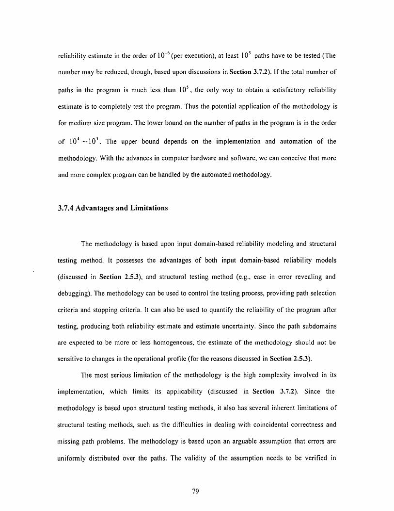
reliability estimate in the order of 10-6 (per execution), at least 105 paths have to be tested (The

number may be reduced, though, based upon discussions in Section 3.7.2). If the total number of

paths in the program is much less than 10', the only way to obtain a satisfactory reliability

estimate is to completely test the program. Thus the potential application of the methodology is

for medium size program. The lower bound on the number of paths in the program is in the order

of 10 i-105 . The upper bound depends on the implementation and automation of the

methodology. With the advances in computer hardware and software, we can conceive that more

and more complex program can be handled by the automated methodology.

3.7.4 Advantages and Limitations

The methodology is based upon input domain-based reliability modeling and structural

testing method. It possesses the advantages of both input domain-based reliability models

(discussed in Section 2.5.3), and structural testing method (e.g., ease in error revealing and

debugging). The methodology can be used to control the testing process, providing path selection

criteria and stopping criteria. It can also be used to quantify the reliability of the program after

testing, producing both reliability estimate and estimate uncertainty. Since the path subdomains

are expected to be more or less homogeneous, the estimate of the methodology should not be

sensitive to changes in the operational profile (for the reasons discussed in Section 2.5.3).

The most serious limitation of the methodology is the high complexity involved in its

implementation, which limits its applicability (discussed in Section 3.7.2). Since the

methodology is based upon structural testing methods, it also has several inherent limitations of

structural testing methods, such as the difficulties in dealing with coincidental correctness and

missing path problems. The methodology is based upon an arguable assumption that errors are

uniformly distributed over the paths. The validity of the assumption needs to be verified in

practice. The estimation of p, is a very difficult step in the methodology. Although the Monte

Carlo method proposed in the methodology can produce estimates of the p, 's, it has difficulties

in quantifying the estimate uncertainties. Its probabilistic nature may hinder its acceptance by the

nuclear industry, or some other industries with ultra-high reliability requirements. Some other

alternatives may be needed.

Chapter 4

A Case Study Using the Integrated Methodology

4.1 Introduction

This chapter presents the results of a case study in which the designed integrated

methodology in Chapter 3 is applied to a program used in a nuclear power plant's reactor coolant

system. The program is the generic Signal Validation Algorithm (SVA) used for calculating and

validating the values of parameters of the reactor coolant system. Because we did not use any

automated tool and had to perform the control flowgraph analysis and testing manually, we were

unable to follow the general application strategy of the methodology discussed in Section 3.7.1.

The estimation of the p 's of the program requires the operational profile of the target program,

which is not readily available. The proposed method for the estimation of the pi 's (i.e., the

Monte Carlo method) requires automation and can not be realized by hand. For these reasons the

case study bypassed the estimation of the pi 's and focused upon program testing and the

estimation of 0 using the testing data. The purpose of the case study is not to assess the

effectiveness of the methodology, rather to show the applicability of the methodology. Section

4.2 presents descriptions of the SVA program. Section 4.3 and Section 4.4 discuss the testing

procedures and the testing results, respectively. Conclusions are drawn in Section 4.5.

4.2 The Signal Validation Algorithm (SVA)

4.2.1 Signal Validation Algorithm Features

In the nuclear power industry, many efforts have been devoted to improve plant

performance and availability. An important factor for the success of these efforts is the improved

access to reliable information for the entire plant, especially for safety critical systems. Many

nuclear utilities are installing or upgrading their plant computer systems to provide such a

capability to handle plant data and provide operators and other personnel with data interpretations

that are accurate, extensive, reliable, and useful. The application of these computer systems

provides operators with a ready access to a variety of sensor signals. It permits operators to use an

increased number of redundant, independent measurements in the decision-making process

during normal and emergency plant operations. However, simply displaying all these redundant

measurements is not desirable because it may adversely complicate the operator's mental

processing tasks of data evaluation and analysis. One way to reduce the operators' work load in

comparing, analyzing, and evaluating sensor signals is to apply automatic signal validation

algorithms as a pre-filter to reduce the amount of information passed to the operator and to the

other systems in the plant.

The Signal Validation Algorithm (SVA) of this case study is a generic algorithm that

performs signal validation for the plant processes that contain multiple sensors measuring the

same or closely related process parameters. The algorithm is called generic because it is generally

applicable to all types of parameters. Only slight modifications need to be made for each

particular parameter according to different quantities of the sensors used.

4.2.2 Implementation of the SVA

The specifications and design documents of the SVA were provided by ABB-

Combusting Engineering, a commercial reactor manufacturer firm. A graduate student in MIT,

M. Ouyang, developed formal specifications of the SVA using an Integrated Formal Approach

(IFA) in the 001 language (Ouya95). The primary concern of Ouyang's work is to find errors

and ambiguities in the specifications using formal methods and software development tools. In

other words, it is mainly concerned with producing error-free specifications rather than error-free

code. Since the 001 tool has the capability of generating executable code automatically based

upon the formal specifications written in 001 language, we treated the SVA formal

specifications as a target program and used it for our case study. The owner of the SVA, ABB-

Combusting Engineering, generously permitted us to use the SVA and its supporting

documentation in our case study, however, on a confidential basis. Thus we may not disclose the

SVA code itself. It is worth noting that the formal specifications were developed in order to find

errors in the original specifications of the SVA as part of its developmental process. This example

is not one of the high quality commercial code that is actually used in nuclear power plants. The

001 tool suite is a CASE tool supporting the Development Before The Fact (DBTF) formal

method. Interested readers can find descriptions and applications of the 001 tool in Ouya95 and

Lung96.

The SVA formal specifications written in 001 language have 18 independent modules

and 416 primitive functional statements. Primitive functions are those elementary functions

supported by the 00 tool. Some examples of the primitive functions can be found in Figure 4.1.

Looping structures are extensively used in the program representing the manipulations on

identical elements in a set, i.e., the redundant sensor measurements for the same process

parameter. A typical looping structure is shown in the module AverageGood in Figure 4.1. The

number of paths in the program is considerably much larger than the number of statements. Based

upon a rough estimate, when the number of iterations for each loop is limited to k=2, the total

number of feasible paths in the program is in the thousands. When the number of iterations for

each loop is limited to k=3, the total number of feasible paths in the program in tens of thousands.

It is a desirable feature for our case study because the more paths are available for test, the better

accuracy may be achieved.

4.3 The Testing Process

The testing of the formal specifications is performed in two phases: a modular testing

phase in which each of the modules is completely tested, and an integrated testing phase in which

the entire program is tested.

4.3.1 Modular Testing

Each of the modules in the program is small and contains a small number of paths.

Complete testing is performed for each module to ensure that it has the correct functionality. In

order to show how the complete testing is done, we use a module AverageGood as an illustrative

example. The Fmap (function map in 001 language which represents the relationships between

the primitive functions) of the module AverageGood is shown in Figure 4.1. The input to the

module is SetOl, a pointer to a set of identical sensor measurements. Each sensor measurement

has a quality field to store the quality of the measurement and a value field to store the actual

value of the measurement. The output of the module is output, the average of the sensor

measurements which have good qualities. The module starts from the first element in the set

(statements a-d), checks the quality of the element (statements g-j). If the quality is good, the

value of the sensor measurement is added to the sum of the measurements and the number of

good sensors is incremented by one (statements n-p). Otherwise, the sensor measurement will be

ignored (statements k-m). Statement e checks if the program has reached the end of the set. If it

has not, the Boolean variable AtNull:Sensor(Getitl) has a value of FALSE. The module goes to

the next element in the set and performs the same manipulation (statements f-r). If the end of the

set has been encountered, the Boolean variable AtNull:Sensor(Getitl) has a value of TRUE. The

module exits from the loop, divides the sum of the good sensor measurements by the number of

good sensor measurements, and outputs the average (statements t-v).

Figure 4.2 shows the control flowgraph of the AverageGood module and its expansion

using the FSPT method discussed in Section3.3. Each node in the flowgraph corresponds to one

or more statements in Figure 4.1. The correspondence is shown on the upper right corner of the

figure. Figure 4.1a shows the unexpanded flowgraph. Figure 4.2b shows the expanded

flowgraph after limiting the number of iterations to k=2 (Note that node C is the exit node so that

the maximum number of iterations in Figure 4.2b is two). Since node B in Figure 4.2b has two

incoming edges, each of the nodes B in Figure 4.2b is duplicated resulting in the expanded

flowgraph in Figure 4.3c.

In Figure 4.3c, there are seven independent paths in the expanded flowgraph. The paths

and their sequences are listed in Table 4.1. For each of the paths, the values of the input variables

are generated based upon program predicate analysis. The expected outputs corresponding to

these inputs are obtained based upon analysis of the specifications and design documentation of

the SVA. The path is then tested using the input values and its outputs are compared with

expected outputs. Discrepancies in the comparison indicate the presence of errors and debugging

is then performed. Testing is redone whenever debugging is performed to ensure the correctness

of the modified code. The test case generation, oracle generation, and debugging process are

omitted here because they require deep understanding of the target program.

Output=AverageGood(Set01) CJ*2, J; ---a

Getit l=Locate

InitNo=K

itTotal=K

If reaches the end of the sensor set, stopsand exits; otherwise goes to the next elementin the set and iterates.

OutPut=UntilConMeet (InitNo, InitTotal, Getitl) CO: AtNull: SensorSet(Getitl); ---e -

tput=Do_Next_Element(InitNo, InitTotal, Getitl) CJ*6; ---f

E=Moveto:SensorSet(Getitl); ---g

Val=Moveto:RawConverted:SensorRd(E); -- h

QV=Moveto:Quality:SensorRd(E); --i

N ,Total=Update_All(Ini:No, InitTotal, Val, QV) CO:Is:Good:Quality(QV); -j

um, Total=NonGood(InitNo, InitTotal) I; -k

[~-Total=Clone 1 :Any(InitTotal); -1

Num-Clone 1:Any(InitNo); -m

um, Total=Real_Update(InitNo, InitTotal, Val) CI; -n

Total=Add:Rat(InitTotal, Val); ---o

Num=Add:Nat(

Getit2=Moveto:SensorSet:SensorRd(E); ---q

Getitn=Ncxt

Output=UntilConMeet(Num, Total, Getitn) -r- -s

ut=Real_Ave(InitTotal, InitNo) CJ; ---t

I NoRat=Convert:Rat:Nat(InitNo); ---u

Output=Div:Rat(InitTotal, NoRat); ---v

Figure 4.1 Module AverageGood FMap

LoopingStructure

I I*

Figure 4.2aUnexpandedflowgraph

Figure 4.2bExpanded flowgraphwith limit k=2

Figure 4.2c Expandedflowgraph with node Bduplicated

Figure 4.2 Control flowgraph of the module AverageGood and itsexpansion

Path Number Sequence1 A+B+C2 A+B+D+E+B+C3 A+B+D+E+B+D+E+B+C4 A+B+D+E+B+D+F+B+C5 A+B+D+F+B+C6 A+B+D+F+B+D+E+B+C7 A+B+D+F+B+D+F+B+C

Table 4.1 Paths in module AverageGood

The testing process for all the other modules follows the same procedure. In order to

improve error-revealing capability, multiple test cases are generated for each path whenever

possible. This is achievable in the modular testing phase because the total number of paths in

each module is small enough. In the modular testing phase a total number of 171 paths are tested

and 10 errors are found. 6 errors are syntax errors that are readily detected by 001 consistency

checking capability. 4 errors are control errors that result in errors in the control flow of the

program and are detected by comparing the actual outputs of the module to the expected outputs

by specifications.

4.3.2 Integrated Testing

After the modular testing phase, each module has been extensively tested and is expected

to have fairly low failure rate. Then integrated testing is performed, which treats the entire

program as an integrated system. Our first attempt for integrated testing is to use the same

approach as that in modular testing phase, or that, generates and expands the control flowgraph,

identifies all the paths, generates test cases and expected outputs for each path, then performs the

testing and debugging. However, this approach turns out to be intractable. In integrated testing

the number of predicates along each path increases dramatically, which increases the complexity

of both test case generation and oracle generation. Since we do not have any automated tools and

have to do the testing all by hands, solving a combinations of constraints, even when they are all

linear, turns out to be very tedious. In order to reduce the complexity, we used a different

approach in integrated testing phase. Instead of specifying a path and trying to find the input

values that cause the path to be traversed, we randomly specify some input values and try to find

which path in the program is traversed with these input values. The overall effect of using this

approach is close to a random selection of paths in the program. Since we do not have the pi 's of

the paths, we have to assume that each path is of the same importance (has the same p, 's), the

random selection does not have much adverse effect. Although the new approach helps to avoid

the test case generation problem, we still have the oracle problem, i.e., we still need to generate

the expected outputs for the specified inputs. This makes integrated testing a tedious and time-

consuming process. Our original goal in integrated testing was to test a majority of the paths in

the program so as to analyze the evolution of the tested software reliability estimate as the

number of paths increases. However, as the testing proceeds it becomes clear that the goal is

unachievable because the time and efforts needed are far more than what we can afford. The total

number of paths we managed to test in integrated testing phase is 390, which is only a small

fraction of all the-paths in the program (estimated to be in the tens of thousands). The number of

errors found is zero, which is a much better result than that in modular testing phase. The large

discrepancy may be explained by the assumption that modular testing has effectively eliminated

most of the errors in the program and the reliability of the program has been greatly improved.

4.4 Testing Results Analysis

In this section we will use the Bayesian Updating method discussed in Section 3.6.3.2 to

obtain an estimate of the reliability of the target program using the testing data. The testing data

from modular testing gives a rough estimate of the error content in the program and can be used

to set the prior distribution. The testing data from integrated testing can serve as an evidence to

update the prior distribution. The resulting posterior distribution can then be used for reliability

estimation.

In our analysis we use a uniform prior distribution with a mean at:

M 4S= E[] = - = 0.0234

N, 171(4.1)

where Mm is the number of errors found in modular testing,

Nm is the number of paths tested in modular testing.

Note that we only counted the 4 control errors found in the modular testing phase. The 6 syntax

errors were ignored, because they were detected by consistency checking in the 001 system

before the generation of the executable code. They do not exist in the executable code and do not

contribute to the unreliability of the executable code. The prior distribution is shown in Figure

4.3.

I I

0.0234

0 002 004 0.06

E[O] = 0.0234

S = 0.0445

Figure 4.3 The prior distribution of the case study

The posterior distribution is shown in Figure 4.4.

400 I

fl( 0) 200

0 0.02 0.04 0.06

0

E[O] = 0.00255

8 = 0.00934

Figure 4.4 The posterior distribution of the case study(N=390,'M=O)

From Figure 4.4 we see that the estimate of the failure rate of the program before testing

is 0 = 3* 10- 3 , which corresponds to a failure probability of 3* 10- 3 per program execution.

From Eq. (3.44), the failure rate of the program after testing, ,, is given by the relationship:

Oa = (1- P)6 . (4.2)

The reliability (per execution) of the program after testing is given by the relationship:

R=1 -(1 - )8 . (4.3)

Because we only tested a small fraction of all the paths in the program, , is expected to be very

small. We approximately have 0, = 0, and R -- 6 = 0.997. Although it is far from meeting

the ultra-high reliability requirement, it is a fairly good result considering the fact that we only

tested a few hundred of paths, a small fraction of all the paths in the program.

4.5 Conclusions

The primary conclusion drawn from this case study is that automation is essential for

practical application of the proposed methodology. Even for a relatively small program (416

functional statements) the complexity in identifying, analyzing, and testing all the paths soon

becomes intractable by hand. The second conclusion is that the estimation of the p, 's is very

important for the application of the methodology. Without the p, 's we lose the opportunity of

improving the efficiency of the testing process (maximizing P ), and can not obtain an accurate

reliability estimate (P, can not be obtained with high accuracy). Finally, although we were not

able to follow the general application strategy of the methodology, we did apply part of the

methodology to a sample program and obtained a reasonable result. We believe that after further

refinement and provided with necessary supporting tools, much better results can be obtained

using the proposed methodology.

Chapter 5

Conclusions and Future Work

5.1 Conclusions

Safety critical software is required to have ultra-high reliability. The most widely used

and most powerful method for ensuring high software quality and reliability is testing. An

integrated methodology is developed in this study for reliability improvement and assessment of

safety critical software through testing. The methodology is based upon input domain reliability

modeling and structural testing method. It possesses the advantages of both input domain-based

reliability models and structural testing method. The methodology can be used to control the

testing process, providing path selection criteria and stopping criteria. It provides a systematic

mechanism to quantify the reliability and estimate uncertainty of the software after testing. In the

thesis the underlying reliability model of the methodology is first presented. Then each element in

the model is discussed. Feasible methods for quantifying each of the elements are presented.

Their advantages and limitations are addressed. The general application strategy of the

methodology is then formulated. The potential applications, advantages and limitations of the

methodology are summarized. Finally a case study is performed applying the methodology to a

sample program to show its applicability.

Software testing and reliability quantification is a very complex process. The primary

concern of the study is not to provide an immediate solution to all practical difficulties (such as

the automatic path generation and test case generation), rather to set up a framework of a new

software reliability quantification methodology. The goals of the study are to reveal what are

involved in software reliability quantification, to show where the difficulties are and how they

might be overcome, and to give guidance for future improvement. Due to limited time and

resources, we were not able to explore in detail many important issues in software testing and

reliability assessment, such as imperfect debugging, error consequences, and domain testing

strategy. We did not actually automate the proposed methodology although we claim that

automation is essential for its application. All these are left for future research. Despite of all the

limitations, we believe that the methodology constitutes a new and promising technique for

software reliability assessment, especially for safety critical software. After further refinement

and automation, the methodology should be able to produce high reliability estimate with high

accuracy.

5.2 Future Work

First, efforts need to be devoted to automate the entire methodology so that it can actually

be applied to medium size programs. Secondly, Monte Carlo method has several undesirable

features and alternative methods for the estimation of p, need to be explored. Thirdly, although

the methodology models the debugging process using Eq. (3.23) and Eq. (3.25) and can account

for imperfect debugging, the two equations may be overly simplified and may not represent the

reality. More complex mechanism may be needed to model the effect of imperfect debugging.

Fourthly, error consequence analysis can be introduced into the methodology so that the software

can be treated in a similar way as the hardware in Probabilistic Risk Assessment (PRA). Finally,

the performance of the Bayesian updating method needs to be analyzed and the underlying

assumptions of the Bayesian updating method need to be verified in practical applications.

References

Abde86 A.A. Abdel-Ghaly, P.Y. Chan, B. Littlewood, "Evaluation of competing softwarereliability predictions", IEEE Transactions on Software Engineering, Vol.SE- 12,No.9, pp950-67, Sept. 1986

Angus80 J.E. Angus, R.E. Schafer, A. Sukert, "Software reliability model validation",Proceedings ofAnnual Reliability and Maintainability Symposium, SanFrancisco, CA, Jan. 1980, pp 19 1- 19 3

Barf69 N.C. Barford, Experimental Measurements: Precision, Error and Truth, Addison-Wesley Publishing Company, Inc., UK, 1969

Basi87 V.R. Basili, R.W. Selby, "Comparing the Effectiveness of Software TestingStrategies", IEEE Transactions on Software Engineering, Vol. SE-13, No. 12,pp 278-1294, December 1987

Basin74 S.L. Basin, "Estimation of software error rate via capture-recapture sampling",Science Applications, Inc., Palo Alto, CA, 1974

Beiz90 B. Beizer, Software Testing Techniques, Van Nostrand Reinhold, USA, 1990

Bhat94 A.K. Bhattacharjee, A. Seby, G. Sen, S.D. Dhodapkar, "CLAS: a reverseengineering tool", First International Conference on Software Testing,Reliability and Quality Assurance, New Delhi, India, Dec. 1994, pp 126-130

Brown92 D.B. Brown, R.F. Roggio, J.H. Cross 11, C.L. McCreary, "An automated oracle forsoftware testing", IEEE Transactions on Reliability, Vol. 41, No. 2, pp272-80,June 1992

Bust94 B.S. de Bustamante, T. Sistemas, "Software reliability modelling: a Poisson typemodel ", Proceedings of the Fourth European Conference on Software Quality,pp312-31 9, Basel, Switzerland; 17-20 Oct. 1994

Chen94A M.H. Chen, A.P. Mushur, V. Rego, "A case study to investigate sensitivity ofreliability estimate to errors in operational profile", The Fifth InternationalSymposium on Software Reliability Engineering, Monterey, California, Nov.1994, pp 2 76 - 18 1

Chen94B T.Y. Chen, Y.T. Yu, "On the relationship between partition and random testing",IEEE Transactions on Software Engineering, Vol. 20, No. 12, pp977-980, Dec.1994

Chen96 T.Y. Chen, Y.T. Yu, "On the expected number of failures detected by subdomaintesting and random testing", IEEE Transactions on Software Engineering, Vol.

22, No. 2, pp 109-119, Feb. 1996

Clar76 L.A. Clarke, "A system to generate test data and symbolically execute programs",IEEE Transactions of Software Engineering, Vol. SE-2, No. 3, pp 2 15-222, 1976

Clar82 L.A. Clarke, J. Hassell, D.J. Richardson, "A Close Look at Domain Testing", IEEETransactions on Software Engineering, Vol. SE-8, No. 4, pp 3 80-390, July 1982

Coen90 A. Coen-Porisini, F. De Paoli, "SYMBAD: a symbolic executor of sequential Adaprograms", Proceedings of the IFAC/EWICS/SARS Symposium on Safety,Security and Reliability Related Computers for the 1990s, Gatwick, UK, 30 Oct.-2 Nov. 1990, pp 105-11

Cowa88 P.D. Coward, "Symbolic execution systems-a review", Software EngineeringJournal, Vol. 3, No. 6, pp229-39, Nov. 1988

Craw85 S.G. Crawford, A.A. McIntosh, D. Pregibon, "An analysis of static metrics andfaults in C software", Journal of Systems and Software, Vol. 5, No. 1, pp37-48,Feb. 1985

Cres96 A. Crespo, P. Matrella, A. Pasquini, "Sensitivity of reliability growth models tooperational profile errors", The Seventh International Symposium on SoftwareReliability Engineering, White Plains, New York, Oct. 30-Nov. 2 1996, pp 3 5 -4 4

DeMi78 R.A. DeMillo, R.J. Lipton, F.G. Sayward, "Hints on test data selection: Help forthe practicing programmer", Computer, Vol. 11, pp34-41, April 1978

Dunn86 W.R. Dunn, "Software reliability: measures and effects in flight critical digitalavionics systems ", Proceedings of the IEEE/AIAA 7th Digital Avionics SystemsConference, Fort Worth, TX, USA, Oct. 1986, pp 6 6 4 -9

Duran84 J.W. Duran, S.C.Ntafos, "An Evaluation of Random Testing ", IEEE Transactionson Software Engineering, Vol. SE-10, No. 4, pp438-444, July 1984

Ferg95 R. Ferguson, B. Korel, "Software test data generation using the chainingapproach", Proceedings of 1995 IEEE International Test Conference (ITC),Washington, DC, USA, Oct. 1995, pp 7 0 3 -9

Ferg96 R. Ferguson, B. Korel, "The chaining approach for software test data generation",ACM Transactions on Software Engineering and Methodology, Vol. 5, No. 1,pp63-86, Jan. 1996

Fish96 G.S. Fishman, Monte Carlo.: Concepts, Algorithms, and Applications, Springer-Verlag New York, Inc., 1996

Fran85 P.G. Frankl, S.N. Weiss, E.J. Weyuker, "ASSET: a system to select and evaluatetests", IEEE Conference on Software Tools, New York, NY, USA, April 1985,pp72-79

Fran93 P.G. Frankl, S.N. Weiss, "An Experimental Comparison of the Effectiveness ofBranch Testing and Data Flow Testing", IEEE Transactions on SoftwareEngineering, Vol. 19, No. 8, pp774-787, August 1993

Gaff84 J.E. Gaffney, "Estimating the number of faults in code", Transactions on SoftwareEngineering, Vol. SE-10, No. 4, pp459-65, July 1984

Gall95 M.J. Gallagher, V.L. Narasimhan, "Software test data generation using programinstrumentation", Proceedings 1st International Conference on Algorithms and

Architectures for Parallel Processing, Brisbane, Qld., Australia, April 1995,

pp 57 5-84

Goe178 A.L. Goel, K. Okumoto, "An analysis of recurrent software failures in a real-timecontrol system ", Proc. ACM Annual Technical Conference, ACM, WashingtonDC, pp496-50 0 , 1978

Goe179 A.L. Goel, K. Okumoto, "Time-dependent error-detection rate model for software

reliability and other performance measures", IEEE Transactions on Reliability,Vol. R-28, No. 3, pp 20 6-2 1 1, 1979

Goel82 A.L. Goel, "Software reliability modelling and estimation techniques", Rep.RADC-TR-82-263, Oct. 1982

Goe185 A.L. Goel, "Software Reliability Models: Assumptions, Limitations, andApplicability", IEEE Transactions on Software Engineering, Vol. SE-11, No. 12,ppl 4 1 1-1423, December 1985

Gokh96 S.S. Gokhale, T. Philip, P.N. Marinos, K.S. Trivedi, "Unification of finite failurenon-homogeneous Poisson process models through test coverage", Proceedings.

The Seventh International Symposium on Software Reliability Engineering,

White Plains, NY, USA, pp299-30 7, Nov. 1996

Goos88 G. Goos, J. Hartmanis, Software Reliability Modelling and Identification, Springer-

Verlag, Germany, 1988

Hals77 M.H. Halstead, Element of Software Science, Elsvier North-Holland New York,1977

Harr95 M.J. Harrold, L. Larsen, J. Lloyd, D. Nedved, M. Page, G. Rothermel, M. Singh,M. Smith, "Aristotle: a system for development of program analysis based tools",Proceedings of the 33rd Annual Southeast Conference, Clemson, SC, March

1995, ppl 10-119

Heis93 K. Heisler, Y. Kasho, W.T. Tsai, "A reverse engineering model for C programs",

Information Sciences, vol.68, no. 1-2, pp 155-89, Feb. 1993

Henn83 M.A. Hennell, D. Hedley, I.J. Riddell, "The LDRA software testbeds: their roles

and capabilities", Proceedings of IEEE Software Fair 83 Conference, Arlington,VA, USA, July 1983

Hou95 R.H. Hou, S.Y. Kuo, Y.P. Chang, "Hyper-geometric distribution software

reliability growth model with imperfect debugging", Proceedings of The Sixth

International Symposium on Software Reliability Engineering, Toulouse, France,

pp 195-200, 24-27 Oct. 1995

Howd77 W. Howden, "Symbolic testing and the DISSECT symbolic evaluation system",

IEEE Transactions of Software Engineering, Vol. SE-4, No. 4, pp266-278, 1977

Howd86 W.E. Howden, "A Functional Approach to Program Testing and Analysis", IEEE

Transactions on Software Engineering, Vol. SE-12, No. 10, pp 9 9 7 - 1005,October 1986

Hunt95 J. Hunt, "Testing control software using a genetic algorithm", Engineering

Applications of Artificial Intelligence, Vol. 8, No. 6, pp 6 7 1-80, Dec. 1995

Inam89 H. Inamura, H. Nakano, Y. Nakanishi, "Trial-and-error method for automated test

data generation and its evaluation", Systems and Computers in Japan, Vol. 20,

No. 2, pp78-9 2 , Feb. 1989

Jasp94 R. Jasper, M. Brennan, K. Williamson, B. Currier, "Test data generation and

feasible path analysis", 1994 International Symposium on Software Testing and

Analysis (ISSTA), Seattle, WA, USA, Aug. 1994, pp 9 5 - 10 7

Jeli72 Z. Jelinski, P.B. Moranda, "Software reliability research", Statistical Computer

Performance Evaluation, pp465-48 4 , W. Freiberger, Ed., New York, 1972

Jeng94 B. Jeng, E.J. Weyuker, "A simplified domain-testing strategy",ACM Transactions

on Software Engineering and Methodology, Vol. 3, No. 3, pp254-70, July 1994

Kemm85 R.A. Kemmerer, S.T. Eckmann, "UNISEX: a UNix-based Symbolic EXecutor for

Pascal", Software - Practice and Experience, Vol. 15, No.5, pp439-58, May 1985

Khos90 T.M. Khoshgoftaar, J.C. Munson, "Predicting software development errors using

software complexity metrics", IEEE Journal on Selected Areas in

Communications, Vol. 8, No. 2, pp253-61, Feb. 1990

Korel90 B. Korel, "Automated software test data generation ", IEEE Transactions on

Software Engineering, Vol. 16, No. 8, pp870-9, Aug. 1990

Kore192 B. Korel, "Dynamic method for software test data generation ", Software Testing,

Verification and Reliability, Vol. 2, No. 4, pp203-13, De. 1992

Kore196 B. Korel, "Automated test data generation for programs with procedures",

SIGSOFTSoftware Engineering Notes, Vol. 2 1, No. 3, pp 2 0 9 -1 5, May 1996

Li95 N. Li, Y.K. Malaiya, "ROBUST: a next generation software reliability engineering

tool", The Sixth International Symposium on Software Reliability Engineering,

Toulouse, France, Oct. 1995, pp 3 7 5 -3 8 0

Lipow72 M. Lipow, "Estimation of software package residual errors", TRW, Redondo

Beach, CA, Software Series Rep. TRW-SS-72-09, 1972

Lipow75 M. Lipow, J.R. Brown, "Testing for software reliability", Proceedings of theInternational Conference on Reliable Software, Los Angeles, CA, April 1975,pp518-527

Lipow82 M. Lipow, "Number of Faults per line of code", Transactions on SoftwareEngineering, Vol. SE-8, No. 4, pp4 3 7-9, July 1982

Litt73 B. Littlewood, J.L. Verrall, "A Bayesian reliability growth model for computersoftware", Applied Statistics, Vol. 22, No. 3, pp332-34 6 , 1973

Litt81 B. Littlewood, "A critique of the Jelinski/Moranda model for software

reliability", Proceedings of Annual Reliability and Maintainability

Symposium, pp357-364, 1981

Litt91 B. Littlewood, "Software reliability modelling: achievements and limitations."5thAnnual European Computer Conference on Advanced Computer Technology,Reliable Systems and Applications, pp336-34 4 . Bologna, Italy; 13-16 May 1991

Lu93 M. Lu, S.Brocklehurst, B. Littlewood, "Combination of predictions obtained fromdifferent software reliability growth models", Journal of Computer and SoftwareEngineering, Vol. 1, No. 4, pp303-23, 1993

Lung96 J.R. Lunglhofer, "Complete Safety Software Testing: A formal Method ", ReportNo. MIT-ANP-TR-040, Massachusetts Institute of Technology, January 1996

Luqi94 Luqi, H. Yang, X.Yang, "Constructing an automated testing oracle: an effort toproduce reliable software", Proceedings Eighteenth Annual International

Computer Software and Applications Conference, Taipei, Taiwan, Nov. 1994,pp228-33

Lyu94 M.R. Lyu, J.R. Horgan, S. London, "A coverage analysis tool for the effectivenessof software testing", IEEE Transactions on Reliability, Vol. 43, No. 4, pp 527-35, Dec. 1994

McCa76 J. McCabe, "A Complexity Measure," IEEE Transactions on SoftwareEngineering, Vol. se-2, No.4, pp. 308-320, December 1976

Mich97 C.C. Michael, G.E. McGraw, M.A. Schatz, C.C. Walton, "Genetic algorithms fordynamic test data generation", Proceedings 12th IEEE International ConferenceAutomated Software Engineering,, Incline Village, NV, USA, Nov. 1997,pp307-8

Mill72 H.D. Mills, "On the statistical validation of computer programs", IBM FederalSyst. Div., Gaithersburg, MD, Rep. 72-6015, 1972

Mora75 P.B. Moranda, "Prediction of software reliability during debugging", Proceedingsof Annual Reliability and Maintainability Symposium, pp327-332, 1975

Musa71 J.D. Musa, "A theory of software reliability and its application", IEEE

Transactions on Software Engineering, Vol. SE- 1, pp 3 12-327, 1971

Musa87 J.D. Musa, A. lannino, K. Okumoto, Software reliability: Measurement,Prediction, Application, McGraw-Hill Book Company, USA, 1987

Nels78 E. Nelson, "Estimating software reliability from test data", Microelectron. Rel.,Vol. 17, pp67-74, 1978

Niko95 A.P. Nikora, M.R. Lyu, "An experiment in determining software reliability modelapplicability", The Sixth International Symposium on Software ReliabilityEngineering, Toulouse, France, Oct. 1995, pp 304 - 13

Offu96 A.J. Offutt, J. Pan, K. Tewary, "An experimental evaluation of data flow andmutation testing", Software - Practice and Experience, vol.26, no.2, p. 165-76,Feb. 1996

Ohba84 M. Ohba, "Software reliability analysis models", IBM Journal of Research andDevelopment, Vol. 28, No. 4, pp428-43, July 1984

Omar89 A.A. Omar, F.A. Mohammed, "Structural Testing of Programs: A Survey", ACMSIGSOFTSoftware Engineering Notes, Vol. 14, No. 2, pp62-70, April 1989

Otte81 L. Ottenstein, "Predicting numbers of errors using software science", PerformanceEvaluation Review, Vol. 10, No. 1, pp157-67, 1981

Ouya95 M. Ouyang, "An Integrated Formal Approach for Developing Reliable Software ofSafety-Critical System", Report No. MIT-ANP-TR-035, Massachusetts Instituteof Technology, August 1995

Pasq96 A. Pasquini, E.D. Agostino, G. D. Marco, "An input-Domain Based Method toEstimate Software Reliability", IEEE Transactions on Reliability, Vol. 45, No. 1,pp95-105, March 1996

Pete94 D. Peters, D.L. Parnas, "Generating a test oracle from program documentation",1994 International Symposium on Software Testing and Analysis (ISSTA),Seattle, WA, USA, Aug. 1994, pp 5 8-6 5

Poti82 D. Potier, J.L. Albin, R. Ferreol, A. Belodeau, "Experiments with ComputerSoftware Complexity and Reliability", Proc. of 6h International Conference onSoftware Engineering, pp94-101, September 1982

Rama76 C.V. Ramamoorthy, S.F. Ho, W.J. Chen, "On the automated generation of programtest data", IEEE Transactions of Software Engineering, Vol. SE-2, No. 4, pp293-300, 1976

Rapps82 S. Rapps, E.J. Weyuker, "Data flow analysis techniques for program test dataselection", Proceedings of the sixth International conference on SoftwareEngineering, Sept. 1982, pp2 72-2 78

Rapps85 S. Rapps, E.J. Weyuker, "Selecting Software Testing Data Using Data FlowInformation", IEEE Transactions of Software Engineering, Vol. SE-11, No. 4,pp367-375, April 1985

100

Rich94 D.J. Richardson, "TAOS: Testing with Analysis and Oracle Support ", 1994International Symposium on Software Testing and Analysis (ISSTA), Seattle,WA, USA, Aug. 1994, pp 138-53

Rudn97 E.M. Rudnick, J.H. Patel, G.S. Greenstein, T.M. Niermann, "A genetic algorithmframework for test generation", IEEE Transactions on Computer-Aided Designof Integrated Circuits and Systems, Vol. 16, No. 9, pp1034-44, Sept. 1997

Schi78 G.J. Schick, R.W. Wolverton, "An analysis of competing software reliabilitymodels", IEEE Transactions on Software Engineering, Vol. SE-4, No. 2, pp 1 04-120, 1978

Schn92 N.F. Schneidewind, T.W. Keller, "Applying reliability models to the spaceshuttle", IEEE Software, Vol. 9, No. 4, pp28-33, July 1992

Shoo72 M.L. Shooman, "Probabilistic models for software reliability prediction",Statistical Computer Performance Evaluation, W. Freiberger, Ed. New York:Academic, pp485-502, 1972

Shoo83 M.L. Shooman, Software Engineering. Design, Reliability, and Management,McGraw-Hill Book Company, USA, 1983

Sobo94 I.M. Sobol, A Primer for the Monte Carlo Method, CRC Press LLC, 1994

Tsou93 M.Z. Tsoukalas, J.W. Duran, S.C. Ntsfos, "On some reliability estimation problemsin random and partition testing", IEEE Transactions of Software Engineering,Vol. 19, No. 7, pp687-697, July 1993

Vall94 F. Vallee, A. Ragot, "FIABLOG: a software reliability tool and its application tospace projects ", The Fifth International Symposium on Software ReliabilityEngineering, Monterey, California, Nov. 1994, pp2 96 -3 02

Vall95 F. Vallee, B. Gayet, H. Derriennic, G.L. Gall, "M-elopee: a case tool for softwarereliability study", The Sixth International Symposium on Software ReliabilityEngineering, Toulouse, France, Oct. 1995, pp 38 1-38 6

Webb87 J.T. Webb, "Static analysis techniques and tools", Proceedings of the Conferenceon Software Tools: Improving Applications, London, UK, June 1987, pp4 3-4 9

Weyu91 E.J. Weyuker, B. Jeng, "Analyzing Partition Testing Strategies ", IEEETransactions on Software Engineering, Vol. 17, No. 7, pp 70 3-7 11, July 1991

White80 L.J. White, E.I. Cohen, "A domain Strategy for computer program testing", IEEETransactions on Software Engineering, Vol. SE-6, No. 3, pp247-57, May 1980

Yama91 S. Yamada, "Software Quality/Reliability Measurement and Assessment: SoftwareReliability Growth Models and Data Analysis", Journal of InformationProcessing, Vol. 14, No. 3, pp254-266, 1991

101

Reliability Improvement and Assessment of Safety Critical ...

Documents

Transcript of Reliability Improvement and Assessment of Safety Critical ...