Reliability enhancement for LTE using MPQUIC in a …...As LTE is already deployed worldwide and...
108
6/7/2018 Rasmus Suhr Mogensen Christian Markmøller Reliability enhancement for LTE using MPQUIC in a mixed traffic scenario A novel MPQUIC Selective Redundant Scheduling implementation
Transcript of Reliability enhancement for LTE using MPQUIC in a …...As LTE is already deployed worldwide and...

6/7/2018
Rasmus Suhr Mogensen
Christian Markmøller
Reliability enhancement for LTE using MPQUIC in a mixed traffic scenario A novel MPQUIC Selective Redundant
Scheduling implementation

1

2
Abstract:
Institute of Electronic Systems
School of Information and
Communication Technology
Fredrik Bajers Vej 7
DK-9220 Aalborg Ø
Title:
Reliability enhancement for LTE using
MPQUIC in a mixed traffic scenario
Theme:
Networks and Distributed Systems
Project period:
Master Thesis, 4th semester M.Sc.E.
Project group:
NDS10-1022
Participants:
Rasmus Suhr Mogensen
Christian Markmøller
Supervisors:
Tatiana Kozlova Madsen
Mads Lauridsen
Troels Kolding
Guillermo Pocovi
Page Numbers: 108
Date of completion:
7th June, 2018
Research and development of devices with high level of
automation and flexibility are becoming more widespread.
Especially self-driving vehicles have gained huge
momentum in recent years and as a part of this trend, the
research into vehicular communication has gained
momentum. Some modules require that the communication
must be reliable with certain delivery threshold. This report
investigates the possibility of using transport layer multi-
connectivity with LTE as an access technology in a mixed
traffic scenario, to facilitate such communication. During
the investigation it is deemed that state of the art protocols
such as MPTCP and the newly developed MPQUIC is not
suitable for such a scenario, as its standard scheduling
mechanisms cannot facilitate reliable transmissions in a
mixed traffic application. However, MPQUIC offers a
good basis for a protocol that can handle such scenarios.
We extend the functionality of MPQUIC with a novel
Selective Redundant Scheduler (SRE) that can schedule an
application data source redundantly if needed. The initial
testing in environments with packet loss or varying delay
behavior, based on real LTE measurements, shows that the
novel SRE scheme offers much better reliability than the
standard schedulers in MPQUIC and much better
bandwidth efficiency than a fully redundant scheduler. An
IPR has been spawned based on this novel solution.

3
Preface
This report documents the work done for the Master Thesis in Networks and Distributed Systems at
Aalborg University for group NDS10-1022. The topic of this project is reliable hybrid access
communication using cellular networks. The project started 01.02.18 and ended 07.06.18. This project is
collaborating with Nokia Bell-Labs and in this context the authors would like to thank Troels Kolding
and Guillermo Pocovi from Nokia Bell Labs as well as Tatiana Kozlova Madsen and Mads Lauridsen
from Aalborg University for contextual and academic supervision as well as supervising the entire
project.
The chapters of this part are enumerated as 1, sections as 1.1 and subsections as 1.1.1. Figures and tables
will be enumerated in the order they appear in.
____________________________________ ____________________________________
Christian Markmøller Rasmus Suhr Mogensen

4
Glossary
3GPP 3rd Generation Partnership Program
Ascii American Standard Code for Information Interchange
FIN Finish
HOLB Head of line blocking
IEEE The institute of Electrical and Eletronics Engineers
Kb / s Kilobit per second
KPI Key Performance Indicator
LTE Long Term Evolution
Mb/s Megabit per second
MPQUIC Multipath quick user datagram protocol internet connection
MPTCP Multipath transmission control protocol
ms millisecond
NAT Network Address Translation
OLIA Opportunistic Linked-Increases Congestion Control Algorithm
OWD One way delay
PD priority data
QoS Quality of Service
QUIC Quick user datagram protocol internet connection
RR round-robin
RTT Round Trip Time
SACK Selective Acknowledgement
SCTP Stream Control Transport Protocol
SOTA State Of The Art
TCP Transmission control protocol

5
Contents Introduction ....................................................................................................................................... 7
Facilitating the communication .................................................................................................... 9
Key Performance Indicators ....................................................................................................... 15
Initial problem statement ............................................................................................................ 17
Requirements................................................................................................................................... 18
Functional requirements ............................................................................................................. 19
Technical requirements .............................................................................................................. 20
State of the Art ............................................................................................................................... 21
Multipath transport layer protocols ............................................................................................ 22
Comparison of protocols ............................................................................................................ 27
Problem formulation ...................................................................................................................... 29
QUIC and MPQUIC protocol overview ....................................................................................... 30
QUIC .......................................................................................................................................... 30
MPQUIC .................................................................................................................................... 36
Conclusion on MPQUIC ............................................................................................................ 40
MPQUIC with Selective Redundant Scheduling ......................................................................... 41
Redundant scheduling ................................................................................................................ 41
Selective redundant scheduler .................................................................................................... 44
Changes and considerations to original MPQUIC ..................................................................... 47
Code design and implementation ............................................................................................... 49
Functionality verification ........................................................................................................... 53
Test framework ............................................................................................................................... 55
Test methodology ....................................................................................................................... 55
Testbed implementation ............................................................................................................. 57

6
Test scenarios ............................................................................................................................. 67
Results .............................................................................................................................................. 69
First iteration .............................................................................................................................. 69
Second Iteration.......................................................................................................................... 80
Conclusion on results ................................................................................................................. 87
Discussion and future work............................................................................................................ 88
Enhancing MPQUIC congestion algorithm ............................................................................... 88
Real world testing....................................................................................................................... 89
Retransmission of “old priority data”......................................................................................... 89
Parallelize the path checks for redundancy ................................................................................ 90
Mixed test with both packet loss and delay................................................................................ 90
Conclusion ....................................................................................................................................... 91
Bibliography .................................................................................................................................... 93
Appendix .......................................................................................................................................... 98
QUIC connection setup .......................................................................................................... 98
Network emulation ............................................................................................................... 100

7
Introduction
Self-driving cars, including cars with driver assisting technologies, have gained a huge momentum in
recent years. This is due to the added safety and convenience of such functionalities [1]. As a part of this
trend, the research into vehicular communication has gained momentum as well. Especially in cases
with high automation, as it provides expanded possibilities to everything from active safety applications
to platooning and traffic management [2].
Today’s self-driving cars mostly rely on multiple radar/lidar sensors to navigate safely through the
landscape or assist a driver in doing so. These sensors enable safer driving [1], due to the faster reaction
time, but the cars still have some limitations. These sensors, as well as humans, are all limited to the
information that is within the line-of-sight of the car. This limitation can lead to bad or unnecessary
behavior, an illustration of this limitation can be seen in Figure 1.
Figure 1. Illustration of line-of-site limitation for the red car.
In this scenario, the red car must stop at the intersection as it is unaware of the behavior of the yellow
and blue car. However, if the cars or the transport related infrastructure, such as intersections, could
share information, via wireless communication, the physical area for which information can be obtained

8
becomes larger. An illustration of this can be seen in Figure 2. In this illustration the cars have a
collective field of view that is much greater than the one in the previous illustration. In this case the red
car might not need to stop if it knew information about the yellow car such as its position, heading,
speed etc. as it could, based on this information, determine that it would not intersect with the yellow
car. In general, this extended field of view will potentially increase the flow of traffic through a city.
Figure 2. Illustration of extended field of view.
The orange area is the collective line-of-site of the cars.
This scenario is only one example of how shared information will benefit the decision making of both
humans and self-driving cars and increase in safety in the traffic. As an example, emergency vehicles
would be able to reserve certain roads in the city as well as announcing its presence to other cars much
earlier to get to the destination faster.
In cases where the information can be used to prevent potential accidents, such as alerts about
emergency breaking, critical failures/wrong decision making can lead to severe injuries or casualties.
Therefore, the overall system reliability of the self-driving cars needs to be very high. Because of this it
is of great importance that the information provided by the onboard sensors and other cars is reliable and
interpreted correctly. This not only imposes strict requirements on the system design of the cars

9
themselves, but also on the wireless communication between them, the infrastructure and other network
attached entities, as the validity of the shared information greatly affects the usefulness, especially in
cases with great mobility. This report limits its scope to only investigate the communication aspect of
the system reliability.
Facilitating the communication
Common for the shared information is that the physical area and the number of devices, for which it is
relevant, is often large and diverse. An illustration of the type of communication that can occur can be
seen in Figure 3.
Figure 3. Illustration of the different car related communication types.
Vehicle-to-Vehicle (V2V) is communication between cars. This communication can be either directly
between the cars or through some access point (AP). This could be an emergency break warning.
Vehicle-to-Infrastructure (V2I) is communication between a car and the transport infrastructure. As an
example, this could be the traffic light system in an intersection. This type of communication could be
direct, through an AP or through the network via the AP. This could be commands whether to slowdown
or speedup to regulate traffic flow in an intersection.
Vehicle-to-Network (V2N) is communication between a car and some network attached entity through

10
the AP. This could be diagnostic information of the car, sensor data live mapping or city level traffic
routing.
The proposed technologies to facilitate this type communication the type of communication are existing
technologies such as 802.11p or Long Term Evolution (LTE) and future technologies such as 5G. In
Table 1 the pros and cons for different technologies are presented, however technologies such as 5G is
not investigated as it is not available yet, however it is estimated to be available by 2020 [3].
Access technology Pros Cons
802.11p - Developed specifically for direct
V2V and V2I communication.
- Does not need existing
infrastructure.
- Standard available.
- Offers low latency in low loaded
conditions.
- The need for installation of
802.11p APs for advanced
V2I and V2N type
communication as it is
mainly focused on direct
V2V.
- Potential scalability problems
in scenarios with large device
density.
- Technology not widely
available.
LTE - Larger coverage area.
- Existing cellular can be used for
communication with network
attached devices i.e. it can
enable V2V, V2I and V2N.
- Technology is widely available.
- Better scalability.
- Is not designed specifically
for this type of application
therefore, no direct
communication is available
yet. This means coverage of
cellular infrastructure is
needed for all the presented
communication types.
Table 1. Pros and cons of the different technologies suggested for vehicle related communication [4] [5] [6] [7].

11
As LTE is already deployed worldwide and there is plenty of off the shelf-device that utilizes this
communication technology it is possible to test any solutions that this report may yield in an actual
network as opposed to 802.11p. Therefore, it is it chosen to investigate LTE as a facilitator for the
information sharing.
To better understand whether the existing LTE network is suitable for this kind of communication, it is
necessary to investigate what kind of performance requirement different application may impose on the
connection.
1.1.1 Vehicular communication requirements
Critical applications, such as collision avoidance, require communication with high reliability i.e.
information gets delivered with a certain probability and latency to maintain stability or functionality.
The requirements of the communication are highly tied to the context of where it is being used. As an
example, a map update due to traffic routing is not as important as being alerted about the position and
behavior of other cars or emergency vehicles. In this report we denote the two classes of information:
priority data for mission critical information with a delay deadline and background data for all data
not within this category.
As a basis for the priority data this report uses the Vehicle-to-everything (V2X) terminology and
requirements proposed by the 3rd Generation Partnership Program (3GPP) in “TS 22.185”. These
requirements will be used as a basis for testing and evaluating LTE as an access technology to facilitate
V2X applications. Below are some of the requirement relevant for LTE V2X communication presented
in Figure 3.
• Max 100 ms latency between two cars via the network (V2V)
• Max 100 ms latency between car and infrastructure, such as an intersection (V2I)
• Max 1000 ms latency between car and network entity, such as a remote server (V2N)
• Max 20 ms latency between two cars for crash related information (V2V)
• Messages of up to 1200 bytes at up to 10 Hz transmit rate and event triggered messages (V2X)
The reliability of the above is defined as the probability of a message being received within the deadline
e.g. received no later than 100 ms after it has been transmitted.

12
Since LTE, as previously stated, do not currently possess the possibility of direct communication
between end points, all communication must go through the base station. This wireless link will have a
major impact on the overall performance and thereby the reliability of the communication. Therefore,
we investigate what kind conditions this link can be subjected to as a car moves through the landscape.
1.1.2 Challenges in LTE
As a car moves through the landscape its LTE connection will be subject to different propagation
dynamics, that affect the reliability and performance of the link directly. These dynamics depend on
different factors such as: distance between sender and receiver, shadowing by other object, multipath
propagation in the environment as well as interference from other radio sources.
The scenario depicted in Figure 4 illustrate some of the network conditions, imposed by the connection
properties of LTE, that a car may experience when moving through the landscape.
Figure 4. Illustration of coverage problem. Cars are only covered in color associated circles.
In Figure 4, Car 1 has a connection to the operator providing the red coverage area circles, as such it will
experience a handover when moving from the coverage area of one cell to another. Since LTE uses a
break-before-make handover scheme [8] no information can be send during the switch between cells.
Therefore, the car can experience an additional delay due to the handover procedure between base
stations. Some applications cannot tolerate these outages (e.g. V2V, V2I), as outages may cause service
deadlines to be exceeded, thereby, decreasing the connection reliability. In [9] an empirical analysis of
handover events in LTE along a part of the Danish freeway presented. It is used evaluate the handover

13
impact on reliability to determine whether the current LTE network infrastructure is suitable for use in
critical applications involving autonomous vehicles (AV). The findings of this article suggest that
handover events are often between 40 ms to 60 ms, but can be even longer. When comparing the
findings with the tolerated delays of V2X communication these are close to some requirements and are
exceeding others, which could impact the reliability of such applications significantly, especially if the
target reliability is high.
Car 2 illustrates a case, where the car has good coverage from the blue service provider, and if it were to
have the red provider, it would have been in less good coverage. This case would illustrate when a car is
in good coverage from a provider and will have a good chance of meeting the deadline from the
application.
Car 3 illustrates a case, where a car is outside coverage of its own provider (blue). In this case Car 3 will
experience a lot of packet losses or even a connection failure causing a longer break in service, which
might cause a time critical application to miss its deadline.
Even though the scenarios in Figure 4 are hypothetical examples of LTE conditions, the cases presented
are present in the real world deployments as well. An example of this seen in work that we have done
previously [10]. In Figure 5, is a real-world example of the issues Car 3 has in Figure 4.
Figure 5. Real world example of coverage problems for a Danish provider between Aalborg and Frederikshavn. The
red dot indicates areas with coverage whereas the gap corresponds to no coverage [10].

14
1.1.3 Possible solutions
One could argue that the best solution is to build a network that is specifically designed to facilitate the
types of applications described above, however, this report will investigate whether current networks
can facilitate some of the use case described previously. Using the existing network infrastructure will
not only quicken the deployment of such application, but also contribute to the research and
development of new applications and reduce deployment costs.
A known and possible way to mitigate the issues presented, in the previous section, is to leverage a
multi-connectivity scheme. Multi-connectivity is a way to utilize multiple connections to achieve better
reliability and throughput. Depending on where the scheme is deployed in the network stack, there are
different advantages and disadvantages. In Table 2 is a comparison of multi-connectivity on different
network layers stating the pros and cons for each.
Layer in protocol stack Pro Con
Transport layer - Agnostic of the lower
layers
- Provider agnostic
- Can provide multi-
connectivity end-to-end
- Large control at
endpoints
- Client control
- Not necessarily
optimized for the lower
layers
Network layer - Agnostic of upper and
lower layers
- Can provide multi-
connectivity between
gateways
- Provider controlled
- Requires Gateway at
ingress and egress point
- Not provider agnostic
- No client control
Datalink layer and lower - Can be tailored to
technology for
performance gain.
- Agnostic of upper layers
- Provider controlled
- Requires specialized
equipment
- Requires that all points
of access implements
scheme
- Not provider agnostic
Table 2. Pros and cons for multi-connectivity in different layer of the protocol stack [10] [11] .
When comparing the different techniques as seen in Table 2 and imposing them upon the scenario in
Figure 4, multi-connectivity at the datalink layer and below is not suitable for this scenario as Car 3 will
still experience no connectivity due to the coverage gap. This is also not possible with the network layer

15
approach as this is not provider agnostic. If the transport layer multi-connectivity is applied, Car 3 could
have access through both the red and blue service provider as this agnostic to the provider.
When applying multi-connectivity to the scenario the cars will now experience the following connection
behavior.
Car 3 has no coverage by the blue service provider, but since it also has access to the red service
provider, it will still have connectivity to serve application data without compromising service deadlines
on the application layer.
Car 1 is still in on the edge of the coverage area even with both providers, however by using a redundant
transmitting scheme the application might be able to reach the deadline, since the probability of packet
loss on both links is lower compared to using only one of the links.
Car 2 might, from a reliability point of view, not gain so much as Car 1, but it can still achieve higher
reliability for the application since it also is within coverage of the red provider.
Key Performance Indicators
Based on the finding in Section 1.1 the following Key Performance Indicators (KPI) are defined for the
priority data communication and background communication. These KPIs will be used from this point
onwards when characterizing the communication and its performance. The following KPIs are defined:
reliability, goodput, throughput and bandwidth efficiency.
Reliability:
- The reliability is defined according to the 3GGP in Section 1.1.1, which is the probability of some
message being sent to be received within a certain deadline.
- This itself is highly tied to what this report denotes as one-way-delay (OWD).
o This sub KPI is measured by setting a timestamp in the packet on the sender application side,
and when the receiver receives the packet, it will log the time for receiving the packet at
application level and subtract it with the timestamp from the sender. Only the priority
communication will be characterized using this definition:
𝑂𝑊𝐷[𝑚𝑖𝑙𝑙𝑖𝑠𝑒𝑐𝑜𝑛𝑑𝑠] = 𝑡𝑖𝑚𝑒𝑅𝑒𝑐𝑒𝑖𝑣𝑒𝑑 − 𝑡𝑖𝑚𝑒𝑆𝑒𝑛𝑡
To which the reliability is defined as.

16
𝑅𝑒𝑙𝑖𝑎𝑏𝑖𝑙𝑖𝑡𝑦 = Pr(𝑂𝑊𝐷 < 𝑇ℎ𝑟𝑒𝑠ℎ𝑜𝑙𝑑)
Where the thresholds indicated the latency requirement such as 100 ms OWD.
Goodput:
- The goodput KPI will be used to characterize how much useful information is transmitted via the
connection. Useful information is defined as all application data. The goodput is calculated with the
following formula:
𝑔𝑜𝑜𝑑𝑝𝑢𝑡[𝑏𝑖𝑡𝑠/𝑠𝑒𝑐𝑜𝑛𝑑𝑠] =𝑡𝑜𝑡𝑎𝑙𝑇𝑟𝑎𝑛𝑠𝑚𝑖𝑡𝑡𝑒𝑑𝐴𝑝𝑝𝑙𝑖𝑐𝑎𝑡𝑖𝑜𝑛𝐷𝑎𝑡𝑎[𝑏𝑖𝑡𝑠]
𝐷𝑢𝑟𝑎𝑡𝑖𝑜𝑛[𝑠𝑒𝑐𝑜𝑛𝑑𝑠]
Throughput:
- The throughput KPI gives an indication of the total amount of data being transmitted this includes all
protocol overhead. Throughput is defined as:
𝑡ℎ𝑟𝑜𝑢𝑔ℎ𝑝𝑢𝑡[𝑏𝑖𝑡𝑠/𝑠𝑒𝑐𝑜𝑛𝑑𝑠] =𝑡𝑜𝑡𝑎𝑙𝑇𝑟𝑎𝑛𝑠𝑚𝑖𝑡𝑡𝑒𝑑𝐷𝑎𝑡𝑎[𝑏𝑖𝑡𝑠]
𝐷𝑢𝑟𝑎𝑡𝑖𝑜𝑛[𝑠𝑒𝑐𝑜𝑛𝑑𝑠]
Bandwidth efficiency
- Bandwidth efficiency is defined as the ratio between goodput and through i.e. how much of the
transmitted data contains unique application information. It is defined as:
𝐵𝑊𝑒𝑓𝑓 =𝑔𝑜𝑜𝑑𝑝𝑢𝑡
𝑡ℎ𝑟𝑜𝑢𝑔ℎ𝑝𝑢𝑡∗ 100
The higher the percentage of BWeff the better the bandwidth efficiency. The maximum efficiency is
100% and the lowest is 0%.

17
Initial problem statement
Based the considerations in Section 1.1.3 as well as the findings in [9] it is deemed the transport layer
approach to multi-connectivity would provide the most value. This offer not ease of deployment and
flexibility using multi connectivity it will also function with off-the-shelf equipment without the need to
change the existing LTE network. Furthermore, this also provides the possibility of both operator and
connection diversity, which would mitigate the LTE problems illustrated in Figure 4. Therefore, the
initial problem statement is the following.
How can the transport layer with multi-connectivity, using LTE as access technology, achieve high
reliability for priority data and facilitate background data with high bandwidth efficiency?
It should also be noted that such a solution would be applicable in other scenarios than cars. Cars could
be exchanged for any device is experiencing changing conditions in a network as described in this
section. The network access technology is not limit to LTE either, this is merely an example of a widely
deployed network access technology.

18
Requirements
This section presents the requirements, that we think, an ideal transport layer protocol should fulfill to
deliver a satisfactory performance and be a possible solution to the initial problem statement. This will
be used in conjunction with an analysis of the state of the art to determine whether and which previous
work can be leveraged in a solution that fulfills the presented requirements for the application presented
in Chapter 1.
For a transport protocol to be viable it must be able to provide different Quality of Service (QoS) to
different data sources, depending on the individual requirements of the sources. As stated in Section
1.1.1, priority data have a very strict set of requirements to insure a certain level of reliability for the
application. On the other hand, background data, such as video streaming, software updates, navigation
information, may not require the same level of reliability, but instead a certain goodput to deliver a
satisfactory performance. Therefore, the transport protocol must shape the output data according to these
QoS parameters and the priority of the data sources.
Based on these considerations the following requirements, for the ideal transport protocol, are defined.
These demands are split up according to the MoSCoW [12] requirement model, where “musts” are
requirement for the implementation to function, “should” is something that should be there but is not
critical for the implementation to function, “could” is an application specific feature, and “wont” is
functionalities that cannot exist in the solution. Furthermore, the requirements are split up into functional
requirements and technical requirements.

19
Functional requirements
Musts:
- M1: Be able provide connectivity diversity to priority data such that the challenges in LTE networks
are mitigated. For this to be achieved it must be able to duplicate data across multiple links.
- M2: Be able to ensure data delivery if required. This means that if losses occur the lost data should
still be delivered at some point in time.
Should:
- S1: Be able to work on the general internet and should not be limited to a proprietary network. This
expands the applicability of the protocol as packets might get rejected by middleboxes if they do not
recognize the protocol used [13].
- S2: Be able to priorities data from a priority data source.
- S3: Be able to redirect protocol control information (such as acknowledgements) and retransmission
to other links if necessary. This is beneficial in the case where the original link is experiencing bad
network conditions.
- S4: Be able to offer good bandwidth efficiency for background data. Bandwidth efficiency in this
case is defined according to Section 1.2.
Could:
- C1: Be able to skip the retransmission of old priority data and not wait for reception of old data. Old
data is in this case data that does not provide any contribution to the application.
- C2: Should not retransmit information that has already received on other paths.

20
Technical requirements
Must:
- M1: It must provide a packet delay of at most 100 ms for priority messages
• There are currently no specific number for reliability in terms of the 100 ms delay. We aim for
99.9 %, if the underlying access technology allows it.
While the V2X communication requirements are used as a basis for benchmarking, the delay
requirement cannot be fulfilled if the underlying access technology is not able to provide delay lower
than this target. Therefore, the aim of this ideal protocol is not necessarily just to fulfill the 100 ms target
at 99.9 % but rather deliver the best possible performance given the limitations of the underlying access
technology, as it may still prove useful other applications.

21
State of the Art
This chapter presents State of the art (SOTA) transport protocols that can leverage multi-connectivity
and be used as basis for the ideal transport protocol presented in Chapter 2. The investigated protocols
are: Stream Control Transport Protocol (SCTP), Multipath Transport Control Protocol (MPTCP) and
Multipath Quick User Datagram Protocol Internet Connection (MPQUIC). These are, to the best of the
authors knowledge, the best candidates to a multi-connectivity protocol in the transport layer.
SCTP [14] is a transport protocol like UDP and TCP, but it uses multiple independent streams to send its
data instead of using a single stream, which both UDP and TCP does. However, there are problems
deploying this protocol on the Internet as addressed in [15]. The main problem is, that SCTP is not fully
supported by NATs and other middleboxes on the Internet and SCTP packets are therefore dropped.
Therefore, it requires an update of all incompatible the middleboxes to support SCTP. The fact that this
must be addressed by all parties, including providers, means that cannot be done by the end user alone.
Because of this SCTP will not be further investigated in this report. MPTCP and MPQUIC, however, are
based upon TCP and UDP respectively and do not suffer from problem to the same extend.
In our earlier work [16] we investigated the possibilities of using MPTCP as a hybrid access protocol to
gain better reliability as opposed to TCP. We showed that MPTCP could achieve higher reliability with
the redundant scheduler [17] and proposed a theoretical method for switching between schedulers based
on the estimated Round-Trip Time (RTT) of the available links. However, this work was limited to a
single stream of application data. As MPTCP is a single stream protocol, a mixture of high priority data
and low priority data can suffer from head-of-line blocking (HOLB) [18], therefore, may not be
appropriate for a scenario with a as this can block data to the application, however as it already have
shown to provide reliability via a redundant scheduler, it will still be investigated in detail.
Multipath QUIC (MPQUIC) [18] is based on the QUIC (Quick UDP Internet Connection) [19] protocol.
QUIC can be used on the Internet and is also capable of passing middleboxes, which is one of the many
challenges when designing a new protocol. QUIC is widely deployed on Googles’ servers, and is
estimated to be around 7% of all internet traffic in 2017 [19]. The motivation for adding multipath
functionalities to QUIC is to pool resources together on different paths to create one connection, like
MPTCP. The work of [18] compared MPQUIC and MPTCP under different network conditions, and
they showed that MPQUIC is better at coping with packet losses than MPTCP, since MPQUIC is better

22
at estimating the latency and has better loss signaling. Furthermore, as MPQUIC is a multiplexed
protocol it can handle multiple application data sources with suffering from HOLB to the same extend as
MPTCP.
Based on the SOTA MPTCP and MPQUIC are compared along with their single path equivalent TCP
and QUIC. Even though the single path protocols are not a valid solution for multi-connectivity, some
features and functionalities from the single path protocol are directly transferrable to its multipath
equivalent. For this reason, TCP and QUIC will also be examined.
The reliability aspect of mixed traffic (priority- and background data) in the transport layer is not widely
investigated, the prior art [20] [10] [17] mostly focus on one type of traffic per connection and the
performance thereof. Therefore, this report will contribute to SOTA in the sense that both reliability and
bandwidth efficiency is considered for a mixed traffic scenario.
Multipath transport layer protocols
To give an overview of the pros and cons of the discussed protocols found in SOTA, this section will
briefly cover the protocols MPQUIC and MPTCP with their respective single path protocol QUIC and
TCP and state the core basics to make a comparison of them. The overview will only cover topics
relevant to the ideal protocol, See Section 2, and the scenario described in Section 1.
3.1.1 TCP
TCP is a protocol that insures data delivery via receiver acknowledgements. It uses an initial 3-way-
handshake when establishing a connection, thereby introducing extra overhead until data can be
transmitted. After setting up the connection the TCP uses three windows to keep flow- and congestion
control (sender, receiver and congestion window).
TCP was made for wired networks [21] which makes the standard implementation view packet losses as
if a network is congested and therefore reduce the congestion window. This might not always be the
case, since nowadays a lot networks and devices depend on wireless access technologies [21] (e.g. LTE,
Wi-Fi). Wireless network often has more packet losses than wired without the network being congested
in this case standard TCP will misinterpret a packet loss as a congestion and therefore reduce the
capability of the link.

23
If out-of-band data (data that is an independent from the main stream of data) needs to be sent, e.g.
priority data, along with main data (e.g. background data), there is no way of prioritizing this data
without disturbing the in-band data flow. TCP only has the urgent pointer in the TCP header to prioritize
packets up to a certain sequence number, however as described in [22] this mechanism is not meant for
out-of-band data, as this is both not supported by many implementations and the fact preceding data also
gets treated like urgent data. Therefore, it is not recommended to be used for prioritizing single
messages within the same application.
3.1.2 MPTCP [13]
MPTCP is a multipath extension to TCP it can utilize multiple network interfaces simultaneously for a
single connection. MPTCP offers the same functionality to applications as regular TCP, but utilizes
multiple TCP flows for the same data stream. A very important topic in the design of MPTCP is the
backwards compatibility to regular TCP, so that MPTCP can be enabled and fall back to TCP if a host
does not support MPTCP (TCP fallback). The protocol also must follow all the standards of TCP to pass
the middleboxes on the Internet, such as NATs, firewalls and proxies, so a packet does not get dropped
because of a non-supported protocol. The protocol stack of MPTCP is seen in Figure 6.
Figure 6. Simplified MPTCP stack.
The concept of how to setup a connection the same concept as TCP but with slight modifications to
enable the multipath functionality. This means that each additional sub flow has its own TCP flow,
meaning that middleboxes will see each sub flow as a regular TCP flow, and that each sub flow must
make its own 3-way-handshake.

24
MPTCP has an extra 64-bit header to keep track of the sequence numbers for all sub flows i.e. a
connection sequence number. This also means that lost packets can be retransmitted on another sub flow
(it is mapped using the sub flow sequence number in the “Data Sequence Signal” field).
MPTCP decides which sub flow gets which packets using a “scheduler”, and in its current form (v0.92)
it has three different schedulers [23]: redundant, round-robin (RR), and shortest round-trip time first
(SRTTF).
Redundant
- The scheduler sends the same packets on all sub flows in a redundant way. The acknowledgement
from the server can only acknowledge one sub flow at a time, meaning one received packet on a sub
flow results in one acknowledgement to the respective sub flow.
Round Robin
- This scheduler schedules packets in a round robin fashion, meaning each sub flow get a “slice” of
the segments, where the size of a slice can be tuned. One can also specify if a sub flow should be left
unused until the other sub flows’ congestion windows fills up.
Shortest round-trip time first (default)
- The scheduler sends data to the scheduler with the lowest RTT, and when the window is full it will
continue with the next-highest RTT and so on.
MPTCP also introduces a term called “pathmanager” [23], which decides how a host should set up sub
flows. There are four current path managers in its current form (v0.92) which are ndiffports, default,
ndiffports and binder.
Default
- The default path manager does not do anything to create sub flows from the host and the host
will not announce either IPs or create sub flows. However, it will accept the passive creation of
sub flows from the sender.

25
Full Mesh
- Full Mesh path manager will create sub flow in a full mesh fashion among all the available sub
flows. It is also possible to create multiple sub flows for each pair of IP addresses. If a sub flow
closes down after a timeout it is possible to re-create that sub flow.
Ndiffports
- Ndiffports path manager will create N sub flows across the same pairs of IP-addresses, and
modify the source port on the sub flows, thereby differentiating them by the port used.
Binder [24]:
- Binder is a pathmanager that has a proxy based approach as it allows the application to take
advantage of gateway aggregation without requiring any modifications. Binder also supports
flexible gateway aggregation without negative effect on the reordering of packets.
3.1.3 QUIC [25]
QUIC (Quick UDP Internet Connection) is a UDP based protocol, which provides a multiplexed and
secure transport protocol for application. QUICs development is inspired on multiple protocols such as
TCP and SCTP. QUIC also takes middleboxes and operating systems into account by using UDP
encapsulation thereby making it more deployable. QUIC authenticates all its headers and it also encrypts
all its data including its signaling. This allows for QUIC to evolve without having to worry about
middleboxes, as these will not be able to read the changes in the signaling, and just a UDP packet with
an encrypted payload.
QUIC has the advantage, that it is not bound by the UDP 4-tuble (Source port, Source IP, Destination
Port, Destination IP) but a QUIC connection ID, which makes it more resilient to IP changes or NAT
rebinding – this is called connection migration.
QUIC sets up its connection by the crypto handshake, and can send data after one RTT (1-RTT) or
immediately (0-RTT) depending on the level of security necessary to communicate. Each QUIC
connection is identified by a unique connection ID which is established during the handshake.
QUIC connection operates in frames for each type of data, meaning that data, acknowledgement and
various signaling has its own frame which can be packed into a QUIC packet. Each of these frames can
belong to different QUIC streams, but these streams will still belong to the same connection and behave

26
independently of each other. This means that if a stream is experiencing packet loss, the other streams
will not necessarily be affected by this. These streams can be mixed in the QUIC packets sent, meaning
that a single QUIC connection can have more than one stream from an application sending different
information. These streams can also be prioritized if necessary, making the stream with the higher
priority fill up the QUIC packet before the other streams.
3.1.4 MPQUIC [20]
MPQUIC is a multipath extension to QUIC and can, just as MPTCP, utilize multiple links for the same
connection. The buildup of MPQUIC can be seen in Figure 7, which also shows that it can be compared
with the buildup of MPTCP.
Figure 7. Simplified MPQUIC stack.
Figure 7 shows how each sub flow is a QUIC connection, meaning that each path will have its own
packet numbering and path specific information to transmit.
Before an MPQUIC connection can be set up, the initial connection must be completed on “stream 0”,
just like single path QUIC. When the connection is set up, MPQUIC can use as many paths as
negotiated in the initial connection startup. Each path is in MPQUIC is identified with the UDP 4-tuble
and a Path ID just like a QUIC connection. Each packet after the connection setup contains the explicit
Path ID of the path it belongs to in the public header.
MPQUIC utilizes the frame structure from QUIC to send data, so if a packet is lost on a link, it does not
necessarily mean it will be transmitted on the same link. This also means that MPQUIC does not need
sequence numbering other than the packet numbering on the individual paths, since it is all frame based

27
on the streams. This is beneficial since MPQUIC might experience reordering of packets when it faces
links which has different latency, so to avoid acknowledgement block on the different links, each path
keeps its own monotonically increasing packet number.
The packet schedulers currently implemented [20] are SRTTF and RR scheduling and function as
MPTCP schedulers described in Section 3.1.2, however, redundant scheduling scheme does not exist.
Comparison of protocols
Various transport protocols with multi-connectivity capabilities have been researched and examined.
The viable candidates for the ideal protocol, presented in Section 2, MPQUIC and MPTCP can both
solve the single path issue, since they can utilize the concepts of multi-connectivity to potentially gain
reliability by utilizing the multiple links simultaneously. A comparison of the two protocols can be seen
in Table 3, where possibilities and further development has been prioritized.
Redundant
Scheduling
across paths
Prioritize
traffic from
application
Resilient to
changes
Reliable
protocol
Head of line
blocking
level
MPTCP Yes No No Yes Connection
MPQUIC No Yes Yes Yes Stream
Table 3. Comparison of MPTCP and MPQUIC
As seen in Table 3, the possibilities and limitations of an application is depending on the underlying
transport protocol. The table is explained by each of its possibilities:
- Redundant scheduling across paths
• This is an important feature to achieve high reliability for data which e.g. has a deadline. In their
current form MPTCP is the only one supporting redundant scheduling of packets, making it the
more reliable than MPQUIC since it can utilize all available paths to transmit the same data,
whereas MPQUIC cannot.
- Prioritize traffic from same application
• MPTCP cannot prioritize the traffic within the same application, meaning if a priority data is
scheduled, it would have to wait for every other packet to depart before it can be sent due to the
FIFO principal in TCP. The packet queue can be large depending on the amount of background

28
traffic, meaning that the deadline might be exceeded before the packet is sent. MPQUIC can
handle this, since MPQUIC can have a separate stream for priority data, which can be prioritized
to be sent before any other data.
- Resilient to changes
• MPTCP is a kernel implemented protocol, which means that customizing it would require
changing the kernel protocol every time changes are made, which is very time consuming.
Furthermore, middleboxes in the Internet can see the changes to a TCP packet, and might drop it
if the changes made are not compatible with the legacy TCP implementation, making it harder to
make changes.
MPQUIC is implemented in various languages, making it more accessible to change and
recompile. Furthermore, QUIC is based on UDP and is encrypted, meaning that changes made in
the encrypted QUIC header cannot be seen by middleboxes. Also, since middleboxes will see it
as a UDP connection, and the rest as an encrypted application, they will not have any reason to
drop the packets.
- Reliable data transfer
• Both MPQUIC and MPTCP are reliable in the sense that they both guarantee that data will be
delivered to the application in order and that the full amount of data is delivered, given that the
connection is not interrupted.
- Head of Line blocking
• Head of line blocking (HOLB) is a phenomenon that can have major impact on the perceived
latency of an application. It occurs when intermediate packets are lost during transmission or
packet arrive out of order. When this is the case, a transport protocol such as MPTCP will hold
back received packets on a link until it has received the missing one, which can result in extra
latency for packets with more important information.
This is phenomenon can also occur in MPQUIC, however, instead of blocking the whole
connection, as with MPTCP, only the stream with missing intermediate data will experience a
block. Therefore, MPQUIC is not as sensitive to HOLB when multiple streams are present,
which is beneficial in a mixed traffic scenario such as the one presented in the report.

29
Problem formulation
After the state of the art has been investigated, a revised problem statement is needed to narrow down
the scope of this work. The initial problem formulation is based on multi-connectivity on the transport
layer, and is as follows.
How can the transport layer with multi-connectivity, using LTE as access technology, achieve high
reliability for priority data and facilitate background data with high bandwidth efficiency?
Based on the investigation of the SOTA there are two protocols that can be used as a basis for the ideal
protocol presented in Chapter 2 . Both MPTCP and MPQUIC has their own shortcomings when it comes
to reliability and further development as written in section 3.2. MPTCP has the redundancy scheduling
which can assure higher reliability, however when background data is present, priority data might still
miss the deadline due to MPTCPs FIFO packet scheduling, as prioritization is not functioning as
intended in TCP. Furthermore, MPTCP can suffer a lot from HOLB on the whole connection, which can
severely impact the reliability. From a practical standpoint, enhancement(s) of MPTCP is also difficult
as this is a kernel implementation, as well as dealing with middle boxes, both of which we have no
experience with.
While MPQUIC has its own shortcomings, such as no redundant scheduler, MPQUIC is customizable
because it is a layer above UDP and middleboxes cannot see changes to the frame headers, since it is all
encrypted. Furthermore, it possesses a build-in functionality of dividing multiple application layer data
sources via different streams, with different priorities. These do also not exhibit HOLB in the same way
as MPTCP, as the HOLB would happen on a stream level and not connection level. Also, existing
implementation such as the one presented in [20], resides in user space which makes development less
complicated.
For these reasons, MPQUIC is chosen as the transport protocol and the revised problem formulation is
therefore:
How can MPQUIC be improved to accommodate an application in an LTE environment, which requires
high reliability for the priority data and high bandwidth efficiency for the background data?

30
QUIC and MPQUIC protocol overview
This chapter contains an overview of MPQUIC and the functionalities and features that are going to be
relevant for our proposed enhancement. MPQUIC is resilient to changes as described in Section 3.2, and
multiple versions exists [18] [26]. This description will use the latest drafts on the IETF website, namely
QUIC update 09 [19] and MPQUIC draft 00 [20]. Update 09 of QUIC differs from the current draft, at
the hand-in of this report, as the QUIC protocol is continuously being revised as of the writing of this
report, though the basic functionalities from QUIC should persist.
As most of the functionalities are directly translated to MPQUIC the following description of QUIC is
also applicable to the MPQUIC protocol. For this reason, an overview of QUIC will be given first, and
after that a description of how MPQUIC makes QUIC a multipath protocol and what changes needed to
be made.
QUIC
The following sections will go over the buildup of QUIC which Section 3.1.3 did not cover. It will
describe how the packet is built on top of UDP and how it transmits data. A QUIC session is the term
used for the overall connection, and it is “in charge” of keeping track of the submodules of QUIC. For
QUIC protocol connection setup see Appendix 12.1.
5.1.1 QUIC Packet
The QUIC packet is the core of the QUIC transport protocol, and is used for every type of
communication, hence all basic packets are build up the same way (with some exceptions since some
fields are optional, see Figure 8). The build-up of a basic QUIC packet is shown on Figure 8.

31
Figure 8. QUIC packet
As seen in Figure 8 there are multiple headers of the QUIC packet, but to a middlebox on the Internet, it
looks like an ordinary UDP packet, with a normal UDP header and a payload. The UDP header is called
“unprotected” seen from QUIC’s perspective, since QUIC does not use the UDP 4-tuple to define its
connection and therefore does not verify it. QUIC uses the connectionID, as seen in the QUIC header, to
define its connection, which also means that the UDP header can change without having to interrupt the
QUIC connection.
In the authenticated header, QUIC has all its mechanisms to make it a reliable protocol. First there is the
public header, which is illustrated in Figure 8 as the red box called “QUIC header”, where QUIC has the
following: Public flags, ConnectionID, QUIC version (optional) and the packet number. The details
of the public flags, QUIC version will not be described in this report, but for the interested reader, it can
be found in [25].
After the public header, QUIC consists of various frames, that contains data or signaling, which is all
encrypted. There can be multiple frames and the frames shown in Figure 8 is just an example of a
payload of frames that QUIC can have. These concepts are explained in more detail in the following
sections.

32
QUIC connection ID:
When a connection has been setup between a client and a server, that connection gets a unique
connection ID. This connection ID is used to identify the connection and will remain the same until the
connection is closed. The advantage of the ID is, that it makes the protocol more resilient to a change of
path, if e.g. a NAT changes or the server changes IP. Instead of having to setup a new connection, one
simply needs to identify the connection with the connection ID, and the exchange of data can continue.
Packet number:
In QUIC the packet number is monotonically increasing, meaning that a packet number is never sent
twice during a QUIC session. This also means that if a QUIC packet is lost, the retransmission of that
packets data will have a higher packet number than the original packet. This functionality is e.g. used by
the congestion algorithm and loss detection. Further details of how these are used is described in Section
5.1.4.
Frames:
A QUIC connection utilizes what are called frames. Each QUIC packet scheduled for transmission will
consist of multiple frames, each having their own purpose. The packet in Figure 8 has two frames which
contains different information which in this case is a stream frame (application data) and an
acknowledgement frame. Depending on the necessity of new signaling information, various other
frames, such as “connection close” or “PING” frame, can be added to the payload of QUIC. The details
of the various QUIC frames will not be described in this report, and for the interested reader, the details
of the frames can be found in [25]. However, it worth mentioning that all signaling has its own type of
frame.
If a frame is lost (in e.g. a packet loss) it is not necessarily retransmitted. The reason for this is that not
all QUIC packets are important to recover e.g. acknowledgement frames, as the acknowledgement
information can be sent in a new frame, which can cover the acknowledgement information from the
lost packet along with new information. QUIC also has packets that are important to recover, such as
stream frames, since this is data which QUIC guarantees delivery of. How QUIC recovers from losses is
described in Section 5.1.4.
33
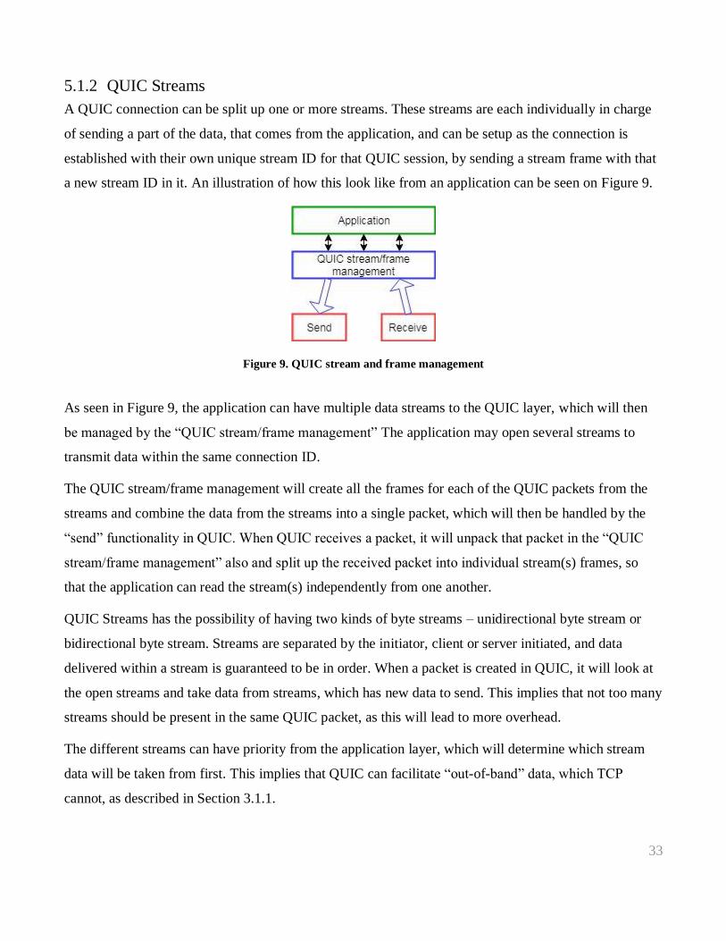
5.1.2 QUIC Streams
A QUIC connection can be split up one or more streams. These streams are each individually in charge
of sending a part of the data, that comes from the application, and can be setup as the connection is
established with their own unique stream ID for that QUIC session, by sending a stream frame with that
a new stream ID in it. An illustration of how this look like from an application can be seen on Figure 9.
Figure 9. QUIC stream and frame management
As seen in Figure 9, the application can have multiple data streams to the QUIC layer, which will then
be managed by the “QUIC stream/frame management” The application may open several streams to
transmit data within the same connection ID.
The QUIC stream/frame management will create all the frames for each of the QUIC packets from the
streams and combine the data from the streams into a single packet, which will then be handled by the
“send” functionality in QUIC. When QUIC receives a packet, it will unpack that packet in the “QUIC
stream/frame management” also and split up the received packet into individual stream(s) frames, so
that the application can read the stream(s) independently from one another.
QUIC Streams has the possibility of having two kinds of byte streams – unidirectional byte stream or
bidirectional byte stream. Streams are separated by the initiator, client or server initiated, and data
delivered within a stream is guaranteed to be in order. When a packet is created in QUIC, it will look at
the open streams and take data from streams, which has new data to send. This implies that not too many
streams should be present in the same QUIC packet, as this will lead to more overhead.
The different streams can have priority from the application layer, which will determine which stream
data will be taken from first. This implies that QUIC can facilitate “out-of-band” data, which TCP
cannot, as described in Section 3.1.1.

34
If a stream hits a byte offset of 262 (meaning it has transmitted a total of 262 bytes), it must terminate and
close the stream, as this is the maximum transmitted bytes per stream. The stream can open again once it
has closed to continue. QUIC also enables flow control on the streams and the overall connection has a
flow controller to achieve both fairness for across streams but also to enable connection flow control.
This is described further in Section 5.1.3.
When a sender wants to signal that there is no more new data, it sends a FIN flags, which will lock the
offset of bytes being transmitted. This means that the connection will keep on going until the amount of
received data has reached the final offset called “size known”.
5.1.3 QUIC flow control
The QUIC flow control is present to ensure that the receiver is not overwhelmed with data. QUIC has
flow control on two layers: a connection level flow control and a stream level flow control. The connection
level flow control prevents the sender from exceeding a receiver’s buffer capacity for the connection and
hence has the overall view of all the streams and their flow control.
This is also done at a stream level by controlling how much data is being send by the stream based on the
consumption rate at the receiver. A sending stream will only be blocked if the consumption rate and send
rate differs. This mechanism relies on explicit signaling and at the start of a stream, the receiver will
announce a maximum amount of data that it is willing to receive on each stream. As the information gets
processed, a window update frame is transmitted to the sender along with the other QUIC frames.
5.1.4 QUIC Loss Recovery [27]
As mentioned QUIC is a reliable transport protocol, which means that when a packet is lost, some
mechanisms must be able to recover the lost information. This section will describe how QUIC recovers
from a loss in different situations to ensure data delivery.
QUICs congestion algorithms and recovery mechanisms are highly based on TCPs congestion
algorithms and recovery mechanisms. As mentioned before, QUIC does not have to retransmit every
packet, as it is only on a frame level, also not every frame is retransmitted (details about re-transmittable
frames can be found in [25]). QUIC enforces a strict increasing sequence number in the packet, where
each packet number only occurs once. When packet losses occur, a retransmission of the necessary
frames will happen, but the sequence number will increase – meaning the higher the sequence number,
the newer the packet. This makes QUIC accurate in its RTT measurements and spurious retransmissions

35
are detected fast due to this mechanism. A mechanism such as Fast Retransmit from TCP [28] can be
applied universally based only on the QUIC packet number. QUIC supports many acknowledgement
ranges, even more than TCPs Selective Acknowledgement (SACK), which makes it quick to recover in
a lossy environment. This means that QUIC is better at handling gaps in the received packets than TCPs
SACK algorithm, as the sender has increase knowledge of missing packets.
QUIC has a “delay” field in the acknowledgement packet, which makes it possible for the sender to see
the delay from it was received until it was acknowledged. This enables the sender to better RTT
estimation and thereby a better estimate of the congestion window. The congestion window that QUIC is
using is the CUBIC algorithm [29] from TCP, however a description of this algorithm out of the scope
of this report.
5.1.4.1 Loss detection
There are many acknowledgements based detection mechanisms for packet loss that QUIC has
implemented from TCP, which are:
Fast Retransmit
- A packet it deemed lost when the receiver has received an acknowledgement that acknowledges
a packet with a packet number higher than the last in order packet, within some threshold (the
threshold is can be tuned).
Early Retransmit
- During the end of a transmission, the threshold to trigger Fast Retransmit might not be met.
Therefore, QUIC enables an alarm for a timer which marks a packet as lost after a given time.
After this timer is exceeded a retransmission will occur from the sender.
QUIC also implements timer-based loss detection for packet loss, also inspired by the TCP loss
detections. These mechanisms include the following:
Retransmission Timeout (RTO)
- Last resort if all other loss detection schemes fails to recognize the loss. A timer is set for every
packet, and if the packet is not acknowledged within that time, the packet is deemed lost.

36
Tail Loss Probe (TLP)
- A packet loss at the end of a transmission can be slower to detect with acknowledgement based
mechanisms. To overcome this, an alarm is scheduled at the sender, which triggers a TLP packet
to be sent to evoke an acknowledgement from receiver. If a RTO occurs before two TLP has
been triggered, the TLP will be sent instead of an RTO.
Handshake Timeout
- Handshake packets in a QUIC connection are very critical to setup a connection between two
hosts, so a separate alarm is used on this control stream. If no prior connection has happened a
static value of 100 ms (as of February 2018) is used as RTT, otherwise the smoothed RTT from
the previous connection is used.
- When the first packet is sent, the sender starts timer. If the timer runs out it must retransmit all its
unacknowledged handshake data. If this step fails one should close the connection as the path is
unsafe (not encrypted)
The loss detection mechanisms are important to the performance of QUIC. When a packet loss occurs,
that packet needs to be recovered as fast as possible. It can be very costly with an environment where a
there is a lot of packet loss, as this will be expensive for the QUIC session to recover, since the
congestion algorithm QUIC is using (CUBIC) will see a lot of packet loss as a network congestion, and
thereby decrease the congestion window unnecessarily [21].
MPQUIC
In order to make QUIC a multipath protocol some changes and extensions have been necessary. The
work of [20] has implemented changes to QUIC to make it a multi path protocol called MPQUIC. This
section will go over some of the important changes to the QUIC protocol to make the MPQUIC
implementation.
5.2.1 MPQUIC Session
MPQUIC has updated the session build up to support the use of multiple paths for the same session.
Figure 10 shows what other functionalities are needed to have MPQUIC working in the session with
multiple paths, and Figure 11 is the QUIC protocol without the multipath. The MPQUIC protocol in
Figure 10 introduces some extra functionalities to achieve utilization of multiple paths. As described in
5.1 and seen on Figure 11, a QUIC session has stream and frame management before sending and

37
receiving messages. MPQUIC however needs to do some extra management of the paths, but for the
creation of packets. In Figure 10 and Figure 11 are the protocols stacks of MPQUIC and QUIC where
the same colors resemble the same functionality.
Figure 10. MPQUIC session
Figure 11. QUIC Session
As seen in Figure 10, when using MPQUIC, the application will send data to the MPQUIC session, just
like the QUIC session, as the MPQUIC protocol is “invisible” to the application. Therefore, no
application changes are needed (except maybe setting the “MPQUIC” flag to enable the protocol).
In the transport layer, MPQUIC must introduce some extra functionalities to support the use of multiple
paths, which can be seen on Figure 11. The new functionalities are the yellow and gray box called “path
manager” and “scheduler” respectively.

38
Path manager:
The path managers function is to keep track of all paths in the session, since every path is perceived an
individual QUIC connection. This includes keeping RTT and the loss statistics for the individual path, as
these are used to the overall condition of the connection and how each path should be adjusted to
achieve the best performance. These inputs are used in the congestion algorithm for the connection
which will be explained later in Section 5.2.4.
Scheduler:
Another functionality introduced in MPQUIC is the scheduling of packets, which is also shown on
Figure 11. MPQUIC has in its current implementation (draft 00 from [20]) only has round-robin
scheduling and SRTTF scheduling as described Section 3.1.4.
MPQUIC stream/frame handler:
After a path has been selected by the scheduler, the individual path will function as a normal QUIC
connection would, except the stream/frame management now works across paths, this means that some
frames have changed its layout to keep track of the originating path. The session flow controller is also
coupled for all paths as the rules for flow control from QUIC still applies for both stream and connection
level flow control. The changes made to the QUIC header are described in the following sections, where
additional information is needed.
5.2.2 MPQUIC Frames changes
MPQUIC must make some changes to the frames to keep track of the extra information that is needed
for MPQUIC to function. This mainly results in all the headers, that are path specific, to have an extra
path ID field added to the header. Examples for such frames could be the acknowledgement frame or
path information frame, since these are path specific. The change of the acknowledgement frame also
results in, that a QUIC packet can be sent on one link and acknowledged on another link.
If a stream frame is sent on one path and lost, the lost frames can be retransmitted on another path
without making any changes to frame or stream structure, since the stream frames are not path specific.
In conclusion to the frame changes of MPQUIC, the only extra information needed in the existing QUIC
frames is the path ID for path specific frames, which is always the ID of the path from which the packet
originates from. Other than the additional path information, extra frames has been added to add/remove

39
paths and other additional frames to cope with the multi path. The details of these frames are out of the
scope of this report, but can be found in [20].
5.2.3 MPQUIC Connection setup
MPQUIC sets up the connection as QUIC does which is described in Appendix 12.1, and as soon as the
connection has been established on one path, MPQUIC does not need to use the connection setup
routine anymore. MPQUIC does not require a per-path handshake after the initial handshake is done, as
the Connection ID is enough to send data to the receiver. Both sender and receiver can utilize this to
their advantage as MPQUIC is fully symmetrical, meaning they can both start sending on an available
path without setting it up first on a current connection. Adding a new path is simply put in to a frame
with the path information and after that, the path can start transmitting data.
5.2.4 MPQUIC Congestion Algorithm
MPQUIC must have its own congestion control algorithm to maintain fairness. If the normal QUIC
congestion algorithm is used, MPQUIC would be able to increase its window way faster, due to its
multiple connections and this violates the fairness principal that each overall connection should have the
same bandwidth. Therefore, the congestion algorithm must be coupled across multiple paths. Figure 12
illustrates how the impact of a coupled congestion algorithm with affect the performance of the
MPQUIC protocol.
Figure 12 [30]. Two connections within a bottleneck. Connection 1 has a multipath transport protocol and connection
2 has a single path transport protocol
As seen in Figure 12 the presence of a coupled congestion algorithm is important. If Connection 1 had a
single path congestion algorithm, it could get up to 2/3 of the connection, whereas Connection 2 would

40
only have 1/3. When designing transport layer congestion algorithms, one must take fairness into
account, which is why the coupled congestion window is present in MPQUIC. The basic idea is to make
the multipath connection less aggressive, such that the congestion algorithm in both Connection 1 and
Connection 2 will converge towards the same, hence they split the connection fairly.
MPQUIC uses a coupled congestion control algorithm from MPTCP called Opportunistic Linked-
Increases Congestion Control Algorithm (OLIA) [31] to adjust the overall congestion window, which
creates fairness. OLIA is based on NewReno but will create fairness across multiple links that are
coupled together. Even though each path will maintain its own congestion window, the OLIA algorithm
will make sure it is not too aggressive towards single path algorithms and split the congestion window
fairly across paths. According to the work of [32] OLIA satisfies the design goals of MPTCP, which is
the transport protocol it was designed for. OLIA increases its window based on two factors: optimal
resource use by utilizing Kelly and Voice’s algorithm [33](an algorithm for load balancing) and
responsiveness by measuring the number of transmitted bits since the last packet loss.
The drawback of this congestion algorithm is the response to a packet loss, as a packet loss is seen as a
congested network. Since the algorithm is based on NewReno, the behavior of OLIA has a similar
behavior to packet loss, it handles by reducing the congestion window. Therefore, it may not perform
well in a wireless or heterogeneous network such as LTE [21].
Conclusion on MPQUIC
MPQUIC has a lot of the functionalities needed facilitate the ideal transport protocol presented in
Section 2. It offers reliable data delivery in the sense, that all data is guaranteed delivery if the
connection remains and offers a multiplexed framework to priorities and mix different traffic types.
Seen from a priority data point of view, the protocol has some shortcomings, since the current
implementation of MPQUIC does have a scheduler aimed at reliability. To overcome this issue and
increase the reliability for priority data, we propose two different solutions “MPQUIC Redundant
Scheduling” and “MPQUIC Selective Redundant Scheduling” which will be described in Chapter 6.

41
MPQUIC with Selective Redundant Scheduling
Our vision is to use MPQUIC as a basis for the ideal protocol presented in Chapter 2 that can facilitate
the mixed priority and background data in applications, such as the one presented in Chapter 1.
Therefore, we propose and implement two novel scheduling schemes, inspired by the MPTCP redundant
scheduler and MPQUICs multiplexing capabilities. We name these “MPQUIC Redundant Scheduling”
and “MPQUIC Selective Redundant Scheduling”. They both address the reliability shortcomings of the
current MPQUIC implementation and MPTCPs inability to properly support prioritized application data
streams.
The scheduling schemes and their functionalities will be explained in detail in the next sections as well
as the changes needed in the standard MPQUIC implementation, to facilitate the new scheduling
schemes. We will also elaborate on the pros and cons of our proposed schedulers with regards to the
requirements presented in Chapter 2.
Redundant scheduling
The MPQUIC Redundant Scheduling scheme are in many ways be inspired by the redundant scheduler
in MPTCP [23]. The MPQUIC Redundant Scheduling will take outgoing application/stream data and
schedule it on all the available paths, such that all stream data will be sent redundantly. Control data,
such as window updates and path information, will not be duplicated, since a loss of a path specific
frames is deemed unnecessary to send redundantly, as these messages are not assured deliverance and
the fact that this not supported by default MPQUIC. An illustration of the proposed redundancy scheme
with two paths can be seen in Figure 13.
Figure 13 MPQUIC redundant packetization algorithm for two streams

42
Figure 13 shows the basic functionality of the proposed redundant scheduling scheme with two paths
and two streams, where one stream is the priority data and the other stream has background data. The
priority stream will generate the priority messages from the application and send it the MPQUIC
Packetization block, where it will be put into a stream buffer with priority. The background stream has
its data generated from the application also, and when background data is present, it will be sent to the
MPQUIC Packetization block, which will create the packets with the data from both the priority stream
and the background stream. A more detailed description of the MPQUIC Packetization will be explained
later in this Section 6.4.
The results of the MPQUIC Packetization for the redundant scheme, can be seen on Figure 13, where all
application data is duplicated across all available paths. The order of the data in the MPQUIC packets,
after MPQUIC Packetization, is also in the order in which they would be packet in practice. The control
messages for the path is generated first, and after that, the priority stream is checked for data and packed
in to the packet if space is available and lastly, background data will fill out the rest of the packet given
background data is available.
The “C” in the packet is the control frames that MPQUIC must have to signal the other part of the
connection, and during packet creation, these are generated first. These control frames are different from
path to path and it is the only messages that are not sent redundantly. It is also important to note that the
“C” changes for every packet on each path, meaning that every new packet generated on all paths has a
different information in the “C” part of a packet. The “C” packet might not be present, if there is no new
path information either.
Pn is the priority data, which will be filled in first if the packet has space and the send window is
available and this data will be sent redundantly on all available paths. Same goes for Bm, which will be
filled in after the priority data and this will also be sent redundantly across all links. In all cases, if the
packet does not have space for the whole message, the message will be split up into partial messages and
sent along with the following packets.
6.1.1 MPQUIC requirements for redundant scheduling
This section will describe if the functional requirements from Chapter 2 are fulfilled or not for our
MPQUIC Redundant Scheduling proposal. Each functional requirement will be compared with the
proposed solution and how the scheduler can help achieve those requirements:

43
Must:
- M1: The redundant scheduler can provide connection diversity so the M1 requirement is
fulfilled. This is done, since every path is utilized with redundant data from all streams in QUIC,
thereby providing priority data with connection diversity. This requirement is fulfilled
- M2: Since MPQUIC will assure data deliverance and the redundant scheduler still provides this
functionality, this requirement is fulfilled.
Should:
- S1: The MPQUIC protocol works on the internet as previously described, and a change of
scheduler does not change that, so this requirement is fulfilled
- S2: The MPQUIC redundant scheduler can prioritize streams, meaning that if the application
sends priority data on a separate stream from background data, the MPQUIC packetization
algorithm is able to prioritize the traffic. This requirement is fulfilled
- S3: Currently MPQUIC supports this feature, as each path has its own unique ID sent along with
each packet. This ID means that a packet received on a path can be acknowledged on any path.
This requirement is fulfilled
- S4: The redundant will send at least twice the amount of data from the application, and that
excluding the overhead for each packet, to send the whole message. This is not considered
efficient; hence this is not fulfilled.
Could:
- C1: The redundant scheduler currently does not provide a solution for C1, since there is
currently not a functionality to determine whether data is considered “old information”. This
requirement is not fulfilled
- C2: Currently, once data is committed to a path, it has to be sent on this path even though it
might be received on another path. This requirement is not fulfilled.
6.1.2 Conclusion on MPQUIC redundant scheduler
The MPQUIC redundant scheduler will benefit the priority data and can in theory provide better
reliability for priority data than the original implementation of MPQUIC. It fulfills the “must”
requirements, which makes it a feasible solution to test, as the scheduler should be able to provide
reliability for priority data.

44
For the “should” demands, not all the requirements are fulfilled for the redundant scheduler. The
redundant scheduler is very data inefficient which is the drawback from this scheduling scheme. Even
though the requirements demand reliability, this only applies for priority data, which is why the
redundancy for background data is deemed unnecessary. Therefore, this scheduler is deemed acceptable
for the bare minimum for the requirements, however it is bandwidth inefficient in scenarios when the
background data is much higher than the priority data.
The “could” demands are not fulfilled for this MPQUIC Redundant Scheduler; however, these
requirements are not crucial for the system and are requirements to optimize the performance. This does
not change outlook for the future test of the MPQUIC Redundant Scheduler.
Selective redundant scheduler
As described the previous section, the MPQUIC Redundant Scheduler has some shortcomings for
bandwidth efficient requirement for background data. For this reason, we suggest a selective redundant
scheme, where only the priority data will be duplicated. The MPQUIC selective redundant scheduler
will take outgoing application data and schedule it differently depending on the priority set from the
application. If the data demands high reliability it will be sent redundantly exactly as described in
Section 6.1 and the rest of the data will be sent with the SRTTF principal as described in Section 3.1.4.
Control data, e.g. window updates and acknowledgements, will not be duplicated, since a loss of a non-
important frame is deemed unnecessary to send redundantly, as these frames are not assured deliverance
from MPQUIC by default. An illustration of the proposed selective redundancy scheme with two paths
can be seen in Figure 14.
Figure 14 Selective redundant scheduling

45
Figure 14 shows the basic functionality of the proposed MPQUIC Selective Redundant Scheduling with
two paths and two streams, where one stream is the priority data and the other streams has background
data. The concept of MPQUIC Selective Redundant Scheduler is very similar to the MPQUIC
Redundant Scheduling as described in Section 6.1, except the MPQUIC Selective Redundant Scheduling
only applies redundancy for the stream, which has priority data. The background data will send its data
with the default scheduling, which in this case is the SRTTF scheduler as described in Section 3.1.4. The
data in each of the packets and messages (C, Pn, Bm) is also the same as the redundant scheduler from
Section 6.1, hence only the scheduling of Bm packets are changed in the MPQUIC Selective Redundant
Scheduler compared with the MPQUIC Redundant Scheduler.
6.2.1 MPQUIC requirements for selective redundant scheduling
This section will describe if the functional requirements from Chapter 2 are fulfilled or not for our
MPQUIC Redundant Scheduling proposal. Each functional requirement will be compared with the
proposed solution and how the scheduler can help achieve those requirements:
Must:
- M1: The MPQUIC Selective Redundant scheduler is able to provide connection diversity. This
is done, since the priority data is sent redundantly across paths, and the background data uses
every path in a SRTTF fashion. Every path is utilized with data from all streams in QUIC,
thereby providing priority- and background data with connection diversity. This requirement is
fulfilled
- M2: Since MPQUIC will assure data deliverance and the redundant scheduler still provides this
functionality. This requirement is also fulfilled.
Should:
- S1: The MPQUIC protocol works on the internet as previously described, and a change of
scheduler does not change that. This requirement is fulfilled.
- S2: The MPQUIC Selective Redundant Scheduler is able to prioritize streams, meaning that if
the application sends priority data on a separate stream from background data, the MPQUIC
packetization algorithm is able to prioritize the traffic. This requirement is fulfilled.

46
- S3: Currently MPQUIC supports this feature, as each path has its own unique ID sent along with
each packet. This ID means that a packet received on a path can be acknowledged on any path.
This requirement is fulfilled.
- S4: The MPQUIC Selective Redundant Scheduler only sends the priority data redundantly,
which is a must requirement, and the rest is sent with the SRTTF scheduler making the MPQUIC
Selective Redundant Scheduler a more efficient scheduler than the fully redundant. This
requirement is fulfilled.
Could:
- C1: The selective redundant scheduler currently does not provide a solution for S2, since there is
currently not a functionality to determine whether data is considered “old information”.
- C2: Currently, once data is committed to a path, it must be sent on this path even though it might
be received on another path.
6.2.2 Conclusion on MPQUIC redundant scheduler
The MPQUIC selective redundant scheduler will benefit the priority data and can in theory provide
better reliability for priority data than the original implementation of MPQUIC. It fulfills the “must”
requirements, which makes it a feasible solution to test, as the scheduler should be able to provide
reliability for priority data.
For the “should” demands, all the requirements are fulfilled for the selective redundant scheduler. The
scheduler is more data efficient since the background data is sent with the SRTTF scheduler, making the
overhead for background data transmission way less than the redundant scheduler. In conclusion the
selective redundant scheduler is the best fit for the application described in Chapter 1 in theory as it
fulfills all “musts” and “should” most of the requirements set to the transport protocol.
The “could” demands are not fulfilled for this MPQUIC Selective Redundant Scheduler; however these
requirements are not crucial for the system and are requirements to optimize the performance. This does
not change outlook for the future test of the MPQUIC Selective Redundant Scheduler.

47
Changes and considerations to original MPQUIC
To support the changes of a redundant scheduling of a stream, several changes must be made to
MPQUIC, but some functionalities can still support the use of redundant scheduling. The changes and
considerations made to the functionality are listed below:
Flow control
- The flow controller does not need changing as the redundant data will look like a retransmission
of the original stream data, if both packets arrive. The redundant scheduling mechanism does not
count duplicated frames more than once in the flow controller as the flow controller only use the
number of unique bytes. The original MPQUIC can handle the redundant scheduling and hence
the flow controller remains unchanged, however it is import only to register a duplicated frame
once at the sender side.
Packet packer
- The mechanism which puts a payload in to the MPQUIC packets from various streams needs an
update to facilitate the redundant stream scheduling. The original packet packer checks each
stream for available payload, and if some data is available it will put the data in a packet on one
of the paths, which is decided by the scheduler. When the data has been put into the buffer, it
would move it from the stream buffer and into the send buffer.
For the redundant case, the data is not deleted from the stream buffer until all interfaces has
transmitted the data. The changes needed to be made is that it does not move the data to the send
buffer until all interfaces has transmitted the same data.
Priority stream:
- Even though having prioritization of streams is documented in [25], it is not properly
implemented in the current version of MPQUIC as described in Section 5.1.2. Therefore, it is
implemented according to the documentation in the way, that the priority streams are checked
first for data and after that, the other streams are checked in a round-robin fashion to ensure that
there is no prioritization with the remaining streams. Priority streams are identified with a new
priority attribute.

48
Scheduling:
- The scheduling needs to be changed as this is in its current form a loop that first chooses a path
based on the RTT, congestion window etc. and then run the above-mentioned modules with that
path as an input. Therefore, this needs to be changed to iterate over all paths when priority data is
scheduled. This is done by making a method that specifies which stream needs to send redundant
information across paths. This is to make sure that only the information that is desired to be sent
redundant is done so.

49
Code design and implementation
The two proposed scheduling schemes are implemented using the same basic functionality, i.e. a stream
specific selective redundancy redundant scheduling mechanism. A flowchart of this mechanism can be
seen in Figure 15.
Figure 15 Proposed MPQUIC packetization algorithm

50
From Figure 15 it can be seen how the overall MPQUIC Packetization algorithm for the two schedulers.
- First it initializes the connection by setting up the streams. After setting up the connection, the
scheduler will check if the connection has been closed in a loop, and this loop will run
throughout the whole connection.
- It runs into the MPQUIC Packetization loop, where all available paths are looped through one by
one to check if anything is available for transmission. First it will check for control messages for
the specific path, which there will always be space for in the packet, as these control messages
do not take up any send window, and hence does not take up flow control, and they are always
put into the packet first.
- After the generation of control messages, it will check for priority data and background (bg) data
respectively and fill in the stream data if there is space available. The size of the control
messages for each path might be different.
- It checks if the redundant flag has been set for the stream, and if it has, it will schedule the frame
on all paths and if the redundant flag has not been set, it inserts the data normally.
By using this approach, the only thing separating the MPQUIC Selective Redundant Scheduler and the
MPQUIC Redundant Scheduler is how many streams, that sends information redundantly. If one wants
to use the MPQUIC Selective Redundant Scheduler, only the priority stream(s) has the redundant flag,
whereas for fully redundant scheduling, the flag must be set on all streams. No matter the scheduling
scheme the priority stream frame is always prioritized, i.e. placed first in a packet.
There is one important note about this implementation of redundancy. As previously mentioned the
available space left for stream frames in a packet might defer from path to path, since the amount path
specific information can be different. There is currently no way of predicting this as the MPQUIC
implementation iterate over paths in a loop. For this reason, a stream frame may not be fully redundant,
as seen in Figure 16. However, the packet with the least stream frame data, will always be fully
redundant to the path with more stream frame data in it. This still makes it a reliable and redundant
scheduling scheme, as it is still redundant to the extent of the packet with the least amount of stream data
in it. The remaining difference from the two packets still will need to be retransmitted if it is lost hence
is still more reliable than a non-redundant scheduling scheme and comes with a better latency for the
data that arrived, as seen by the “safe” data in Figure 16. This effect, is mitigated for the priority data

51
frame as it will always be placed first in a packet and because the frame 1200 bytes (see Section 1.1.1) is
smaller than the maximum transmittable units and the potential path overhead will not cause it to exceed
the limit.
Figure 16. Duplicated frame on two paths with unequal size. Frame bytes beyond the red line are unsafe, and save
below.
Based on implementations MPQUIC implementation in GO (available on GitHub [34] , which is based
on the implementation of the GO implementation of QUIC which can be found on GitHub [35]), we will
implement our stream specific redundant scheduler as an extension to the existing implementation of the
MPQUIC protocol. In Table 4. a very brief explanation of the functionality of the files, the changes we
have made to implement the stream specific redundant scheduling shown in Figure 15. It should be
noted that to successfully implement the scheduling scheme, it has been necessary to obtain an in depth
understanding of many of the modules of MPQUIC to maintain compatibility, debug and log
performance information.

52
Filename Purpose Changes for our schedulers
Stream.go Defines a stream and associated
methods for handling reading,
writing etc.
Added duplication flag. “Book
keeping” for transmission of
duplicated data such that stream
pointer is moved only when all
duplication have been made.
Scheduler.go Defines the scheduling
algorithms and manages path.
Sort of “main loop” for
MPQUIC transmission.
Added mechanism for
scheduling multiple sending
paths if an open stream has its
duplication flag set and data is
ready.
Stream_framer.go Defines methods for creating
stream frames from different
streams etc.
Added book-keeping for
number of duplications made as
the flow controller only looks at
the amount of unique data
transmitted and received
therefore only the last
duplication affects the flow
control.
Stream_map.go Defines a collection of streams
and method for managing these.
A round robin scheme selecting
streams to get data from.
Added prioritization
functionality such that streams
in a prioritized list always
selected before the “regular”
round robin scheme is active
Table 4 MPQUIC code changes
A functionality verification of the implemented scheduler further explained in Section 6.5.

53
Functionality verification
This section describes the results of the functionality test, i.e. if the implemented solution functions as
intended. As described in rest of Chapter 6 we have been made several contributions to the MPQUIC
implementation. The major contributions are stream prioritization, MPQUIC Redundant Scheduling and
MPQUIC Selective Redundant Scheduling. To verify that our schedulers are working as expected, a
setup of two virtual machines are setup as illustrated in Figure 17.
Figure 17. Verification setup
As illustrated in Figure 17 the verification setup has two virtual machines that will act as a “client” and a
“server”. The client will have two interfaces, which it will use to send a random message using
MPQUIC. The scheduler used on the client for the MPQUIC connection will be either MPQUIC
Selective Redundant Scheduler or MPQUIC Redundant Scheduler in two independent tests, to test the
behavior of the scheduler. To show the behavior of the client and the schedulers, the data from the client
will be logged on the server side, where a print in the terminal will print out the raw packet received
from the client. This print out is verifying the functionality in the way that the raw ASCII packet is
showing which part of the packet is sent redundantly on the different paths.
MPQUIC redundant scheduler verification test:
Figure 18 illustrates that our MPQUIC redundant scheduler works as expected. The red box, which is
the priority stream sent on Stream 3, shows the exact same data for both paths and hence is sent
redundantly across paths. The green box, which is the “background data” on stream 5, shows the exact
same data from both paths on stream 5 and hence is sent redundantly across paths. Figure 18 shows an
example output sent during the verification test, however all the packets in the test was sent with
redundant streams across paths, so the MPQUIC redundant scheduler is verified. The stream numbering
of 3 and 5 is an implementation choice from the work of [35], where opened streams from the client are

54
uneven and the initial stream ID is “3” and increments by 2 every time a new stream is opened. Note
that the actual payload has no meaning, and should not be interpreted.
Figure 18. Debug output from stream data received on server, with MPQUIC Redundant Scheduling.
MPQUIC redundant scheduler verification test:
Figure 19 illustrates that our MPQUIC Selective Redundant Scheduler works as expected. The red box,
which is the priority stream sent on Stream 3, shows the exact same data for both paths and hence is sent
redundantly across paths. The green box, which is the “background data” on stream 5, is only present on
one of the paths and hence it is sent with the SRTTF scheduling. Figure 19 shows an example output
sent during the verification test, however throughout the connection only the priority stream (stream 3)
was sent redundantly and the background stream (stream 5) was sent with SRTTF scheduling. The
streams are not always mixed as shown in Figure 19, as the data on both streams might not available for
transmission at the same time. This means that some packet might only have background data and some
might only have priority data. However, the purpose of the MPQUIC Selective Redundant Scheduler is
still fulfilled, as the priority data is always sent with redundancy and background with SRTTF, so the
scheduler is deemed verified. Note that the actual payload has no meaning, and should not be
interpreted.
Figure 19. Debug output from stream data received on server, with MPQUIC selective redundant scheduling.

55
Test framework
This chapter contains an overview of the framework used to evaluate our novel solutions presented in
Chapter 6. The main goal is to create a testing environment where our novel solutions will be subjected
to different network conditions as well as the condition of an LTE network, as previously presented in
Section 1.1.2. To understand how this is achieved an overview of the test methodology, the test setup
and the test implementation are presented. This includes a description of the connection emulation along
with associated traffic models that is used to emulate priority and background data.
Test methodology
There are multiple ways to evaluate and compare the proposed solution to the SOTA which includes
analytical, simulation, emulation and real-world testing. Each of these methods, however, have different
strengths and weaknesses for testing purpose. The different methodologies are compared in this section,
where the scope of the project is taken into consideration along, with the use of the MPQUIC
implementation, when choosing an evaluation method. Based on these considerations the pros and cons
of the different evaluation methods are presented below.
Analytical:
- The MPQUIC has a lot of components that has an impact on the performance, e.g. link quality,
congestion windows, path information etc. This is very complex to model analytically, so even
though the analytical model is fast to evaluate, the effort that will have to be put in to this method is
simply too time consuming and inaccurate due to the complexity of MPQUIC. This analytical
model is therefore deemed to not be a good candidate for the evaluation of the schedulers.
Simulation:
- Simulation has a lot of advantages to evaluate the schedulers of evaluating MPQUIC, however the
efforts of making an implementation of MPQUIC in a network simulator (e.g. NS3, Omnet) has yet
to be made, which makes it a time-consuming process. Even though a good simulation for MPQUIC
could give good results for the behavior of the schedulers, the time which must be invested into
implementing MPQUIC from scratch into a simulator is deemed to be too time consuming for the
scope of this project. The simulation is therefore deemed to not be a good candidate for the
evaluation of the schedulers.

56
Emulation:
- Emulation has a lot of advantages to evaluate the schedulers of MPQUIC, as the MPQUIC protocol
is already implemented for a real network, hence emulation does not require changes to the protocol.
The cons using emulation comes down to the accuracy of the link models used, but when using good
models, the emulation can give an estimate of how the MPQUIC protocol would behave in a real
network. Therefore, emulation will be deemed a good candidate to test the schedulers, as it requires
minimum implementation to test.
Real world testing:
- Real world testing would be the best way of testing the MPQUIC schedulers, since the other
evaluation methods are trying to come as close to the real world as possible. However, real world
testing is very time consuming for small functionality tests and it can be difficult to single out issues
in the network, as the network will be a “black-box”. To cover all scenarios would demand very
extensive tests, which would demand a great amount of resources. Therefore, making an actual real-
world test is deemed to be too time consuming given the scope of this project.
We choose an emulated evaluation platform evaluate our novel scheduling mechanism as this is the
easiest environment to deploy our already implemented schedulers described in Section 6.4. An
emulation will be able to give a good overview of the MPQUIC behavior using various schedulers, and
we will be able to pinpoint any issues that may arise during testing. We based our emulation around the
conceptual drawing seen in Figure 20.

57
Figure 20. Illustration of the entities in the testbed.
The transport protocol configurations will be interchangeable to compare the newly implemented
scheduling configurations introduced in Chapter 6 SOTA MPQUIC scheduling (the SRTTF scheduler)
in different settings. No change will be done to the lower layer and both the client and server will have
one or more network interface(s). Between the server and a client, there is a box that emulates the end-
to-end network conditions (delay, packet loss, etc.) for each of the interfaces, where the uplink and
downlink is two separate emulations as this is asymmetric in LTE [8]. In the following sections is a
description of the test scenarios along with each of the entities of the conceptual testbed.
Testbed implementation
This section contains an overview of how the testbed presented in Section 7.1 is implemented along with
the various considerations made during the implementation as well as a description of the equipment and
software that has been used or developed. This includes the MPQUIC API, end-to-end network emulator
called Kaunetem and a traffic model used to generate the background and priority data streams. The
“measurement application” itself leverage the framework presented in Appendix 12.2.1

58
Figure 21. Test network. Arrows indicate the direction of the traffic flow.
Below is a list of equipment used to construct the testbed.
• Client, Ubuntu 18.04, kernel 4.5-rc3 with with Kaunetem
o 12 GiB RAM, i5 2500k, Samsung Evo 850 SSD 250 GiB
o 2x Intel 1000 pro gt NIC
• Server, Ubuntu 18.04, kernel 4.5-rc3 with Kaunetem
o 8 GiB RAM, i7 4702mq, Toshiba THNSNF12 128 GiB
o Apple A1277 USB to Ethernet
• Switch, Cisco Catalyst 2490 configured for 100 Mb/s
• Router, LinkSYS WRT54GL
• NTP service for time synchronization, sub 1 ms accuracy.
The client will have two interfaces to be able to use MPQUIC across two links. The client will be
connected to a switch, which has one connection to the server. The server will only have one path to

59
serve the MPQUIC protocol, since the MPQUIC implementation used in this report, only allows for a
single interface to be used.
As seen in Figure 21, there are modules not yet introduced that are present in the test network. The next
sections are going over the concepts of “MPQUIC API”, which is the API from the measurement
software to the MPQUIC protocol, and “Kaunetem” which is the chosen network emulator. MPQUIC
API will be explained in Section 7.2.1, and Kaunetem will be explained in Section 7.2.2 and lastly the
traffic model used in the “Measurement application” will be explained in Section 0.
7.2.1 MPQUIC API
As previously mentioned, the measurement application presented in Section 7.3.1.1 is used as a basis for
the evaluation and the reason for this is that it is actively being developed and used for field
measurements of protocols such UDP, TCP and MPTCP. Therefore, it is within our interest to maintain
compatibility with this application, as this is will benefit future work beyond the scope of this report as
well as increase the exposure of the novel solutions presented in this report, which is why effort has
been used on designing an MPQUIC API. The measurement software is written in C++11, whereas the
MPQUIC protocol is written in GO, so the API is an interface from C++11 to GO, which is fully
supported in GO.
The goal of the MPQUIC API is not only to maintain compatibility with the measurement program, but
also to ease the usage of MPQUIC in an actual application. The basis of the designed API draws
inspiration from the widely used Berkley socket API [36] and the way that a connection is created and
destroyed in a server-client connection flow.
The overview of the MPQUIC API flow can be found in Figure 22 for the server and Figure 23 for the
client. In server connection flow, MPQUIC is first initialized and next it is bound to an IP address
similarly to the TCP API, but instead of listening for an incoming socket connection like TCP, it listens
for incoming sessions, since the socket connection is handled by the UDP protocol. Where it differs
from the TCP API, is that instead of acceptation a single connection with a single stream from the client,
it will also accept multiple streams which will expose the stream(s) as individual connections that can be
perceived as a TCP socket from the application point of view.

60
Figure 22. MPQUIC server API
Figure 22 shows the flow of the MPQUIC connection on the server using our MPQUIC API. The steps
are:
- Initialize MPQUIC
o This step makes sure that the multipath flag is set and that all the settings are valid for the
MPQUIC connection.
- Bind to address
o The server binds an IP and a UDP port, which it will use for the next step.
- Listen for incoming Session connection
o The server will listen on the port and IP, which was specified in the previous step. The
maximum amount of sessions a server can handle is not specified, and hence it can accept
multiple sessions on the same port.
- Accept Stream/Configure scheduler
o When a session has been accepted, the server needs to wait for the client to open a
stream. When a stream is opened a flag is set, indicating if the stream should be sent
redundantly or with the default scheduler.
- Write/read on Stream
o Communication with the streams that are open, exchanging data.
- Close session/close MPQUIC
o This step can either terminate a specific session, or it can close MPQUIC all together,
meaning that it does not listen for anymore sessions and releases the port previously
bound.

61
Using this mimicked TCP approach similar read/write methods are created which instead of a socket
takes a stream ID. The close phase is also very similar, however if the server is closed, the underlying
MPQUIC instance is also closed.
The client side is similar to the server API, however an extra step is necessary as streams each have a
unique socket and that the scheduler needs to configure as well.
Figure 23. MPQUIC client API
Figure 23 shows the flow of the MPQUIC connection on the server client our MPQUIC API. The steps
are:
- Initialize MPQUIC
o This step makes sure that the multipath flag is set and that all the settings are valid for the
MPQUIC connection.
- Connect to server via session
o This step tries to connect to a server with an IP and a port, to open up a session with the
server.
- Create stream/configure scheduler
o The client initiates the opening of streams, so in this step, the client will open as many
streams as it wants (within the maximum stream limit defined in [25]). For every stream
opening, a flag needs to be set indicating whether or not the stream should be sent
redundantly across paths.
- Write/Read on Stream
o Communication with the streams that are open, exchanging data.
- Close Stream/Close session
o Close stream

62
▪ Will close a specific data stream, such that data can no longer be sent until it is
opened again.
o Close session
▪ This will close all streams for the specific session and afterwards close the
session.
7.2.2 End-to-end network emulation (Kaunetem)
This section presents the measurement campaign that will be used as a basis for the variable delay test as
presented in Section 7.3.
The scenarios we want to test our MPQUIC schedulers with are based a multi connectivity solution in
LTE, we conduct a measurement campaign along the Danish freeway, as seen in Figure 24. The test is
conducted using one link from each of the three main providers that exist in Denmark and one extra
using use the same operator to characterize both operator diversity and same-operator diversity. A
further elaboration of the measurement setup can be found in Appendix 12.2.1.
Figure 24. Drive test route, Aalborg → Frederikshavn
The test is conducted using a traffic model that emulate that of periodic V2X messages (100 ms inter-
arrival and 1200-byte payload) presented in section 1.1.1, with no background traffic and using UDP as
the transport protocol. The conditions that these messages experiences will be used to extrapolate the
delay behavior of the network, which is then used as inputs to the emulation environment.

63
Based on the measurements, OWDs are extracted for the individual operators. The different lines
represent different connection where A1 and A2 are using the same operator and will be used for the
variable delay test.
Figure 25. OWD empirical CCDF for uplink with 100 ms packet interval and 1200-byte payload.
By examining the Complementary Cumulative Density Functions (CCDF), there is a difference between
the operators, even when using multiple links from the same operator (A1, A2). This indicates that there
is a potential gain by using the different links in a multi-connectivity scheme both with and without
operator diversity, however this is under the condition that not all links experiences the same conditions
at the same point in time, hence we want uncorrelated behavior across the links.
To investigate the potential gain of using multi connectivity, a pseudo redundant scheduling scheme is
emulated in Figure 25, by taking the lowest OWD for each of the received packet IDs across all the
links, which is the ‘Combined’ line result of that OWD. Based on the ‘Combined’ line, it is clear that a
combination of connections provides a theoretical significant improvement in terms of OWD seen from
an application point of view.

64
The goal of measured LTE statistics is to use them as a basis for the emulated network conditions.
Therefore, difference tools that can be used to recreate these network delays are investigated in
Appendix 12.2.3. Based on this investigation, Kaunetem will be used as a basis of the network
emulation in the testbed, as it offers all the functionalities necessary to facilitate the test scenarios
presented in 7.3. However, due to the restriction of only having a single downlink interface from the
server, the type of network emulation that can be achieved with Kaunetem is limited, since Kaunetem
only supports the use of one network trace at a time, and hence the server cannot be emulated as having
multiple operators. It can only apply conditions (packetloss, delay etc.) on outbound traffic. Therefore,
unless otherwise stated, all results will be obtained by applying probabilistic conditions to the client
interfaces (uplink) and deterministic conditions to the server interface (downlink). However, this will
still achieve a variable RTT on the client, which is the desired behavior.
For the packet loss, Kaunetem will be imposed on all links on both server and client, however these
packet losses are not based on real-world measurements but a random packet drop, as described in
Section 7.3.
7.2.3 Traffic Model
This section contains a presentation of the traffic models that will be used for the background and
priority data.
Priority data traffic model. The traffic model that will be used for the priority data will be created
according to the periodic V2X messages, i.e. 100 ms interarrival time and a message size of 1200 bytes,
see Section 1.1.1. The traffic model of these messages is shown in Figure 26.

65
Figure 26. Traffic generated in a period of one second for priority data
This kind of traffic generator will produce an average 96 Kb/s worth of priority data excluding the
overhead for each message. This traffic model will be the base of the priority data sent in the test
Background data traffic model. The traffic model of the background data is not determined or defined
by any standard as such and the exact behavior depends heavily of which type of application that
generates the traffic. As an example, FTP traffic would probably deliver a sporadic traffic load that
which duration would depend on the file being downloaded. On the other hand, a video stream would
provide a regular, but not necessarily constant flow of data. Since the goal is to evaluate the protocol in a
network that is changing over time, as well as compare it against other protocols, a predictable and
regular dataflow is preferable. To do this, a traffic generator is created that can deliver an average bitrate
of a specified amount, in a predictable manner. This generator creates chunks of data 12500 bytes (100
Kb) at a certain rate that in turn corresponds to the desired average bitrate. The packet generation
interval is therefore defined as based on packet size:
𝑝𝑎𝑐𝑘𝑒𝑡𝑖𝑛𝑡𝑒𝑟𝑣𝑎𝑙 =100𝐾𝑏
𝑏𝑖𝑡𝑟𝑎𝑡𝑒
This kind of traffic generator will have a pattern as depicted in with an average of bandwidth of 1 Mb/s
and a departure rate shown in Figure 27.

66
Figure 27 Departure of background data for 1 second
Mixed priority data and background data:
If the traffic from the two generators are combined the resulting traffic will have the following pattern.
A pattern of traffic can be seen in Figures Figure 28 and Figure 29, where they have a different
departure time:
0
2000
4000
6000
8000
10000
12000
14000
0 200 400 600 800 1000
Data
(byte
s)
Time (ms)
Traffic model, background stream

67
Figure 28 Mixed traffic same departure interval, desired
behavior
Figure 29 Mixed traffic different departure interval,
undesired behavior
As seen on Figure 28 and Figure 29 it is important that the background data and the priority data has a
departure time that are non-divisible from one another. On Figure 29 the interval time for departure for
the two streams are the same, which can result in a situation where the traffic is never mixed. If the
bandwidth is high enough to facilitate the background data before the departure of a priority packet, the
wanted behavior of mixed traffic might never occur. For this reason, it is beneficial to change the
departure time for the background data (hence change the amount of background data sent), to minimize
this behavior and get more packets with mixed traffic from both streams.
Test scenarios
This section contains a description of the test scenarios in which the implemented novel schedulers will
be evaluated and compared against the SOTA SRTTF scheduler. The schedulers that will be tested is
therefore the SRTTF, MPQUIC Selective Redundant Scheduler and MPQUIC Redundant Scheduler.
The scenarios are split up into two parts, where the impact of two key factors are tested: various packet
loss probabilities with fixed packet network delay and a varying network delay with no packet loss.
- Packet loss scenario
The packet loss setup will be conducted to evaluate the performance of the schedulers in network
scenarios with packet loss. The packet loss scenario will be conducted with a fixed delay to rule
out any impact a delay may have, such that all schedulers will experience the same conditions.
The packet loss test is expected to give information about the loss recovery and behavior of the
congestion for the MPQUIC and how this affects the streams. At the end , this is compared to the

68
requirements in Chapter 2, in order to make an estimate of how the scheduler can mitigate the
effect of the packet losses.
The packet loss percentages will be tested with the following percentages: 0%, 1%, 2% and 5%.
The reason for choosing these percentages is to see how these are impacted by a gradually
increasing packet loss and how well the schedulers will perform in different packet loss
environments.
- Varying OWD scenario
The OWD test will be conducted to evaluate the performance of the schedulers in a network with
varying uplink OWD and a deterministic downlink delay, due to implementation limitation
explained in Section 7.2.2. Each path uplink has a varying OWD over time. The OWD test will
be conducted without packet losses to rule out the impact of packet losses to the varying OWD.
The OWD test is expected to give information about how varying delay will impact the streams
and how efficient the schedulers are able to handle paths that will experience varying latency.
The varying OWDs will be based on real world measurements made on the LTE network in
Northern Denmark to emulate a real LTE network. See Section 7.2.2.
The scenarios described in this section will give an overview of the performance of the different
schedulers and how the individual parameter will affect the performance of streams. These tests can be
used to estimate the overall performance according to the requirements set in Chapter 2 and to give an
idea of how to further enhance the performance of the implemented scheduling mechanisms.

69
Results
This chapter presents the results obtained for the test scenarios described in Section 7.3. i.e. packet loss
test, and variable OWD test. This section will present various plots to explain the results and interesting
findings along the way. The results are divided into two iterations as some interesting problems were
discovered during the first one and the corrected in the second iteration.
First iteration
This section contains the results for the first iteration, where both packet loss and delay will be tested.
Not all test results are presented as we already in an early stage of the testing discovered that the
MPQUIC congestion interfered with the functionality of the novel scheduling solutions presented in
Chapter 6.
8.1.1 Impact of packet loss
This section presents the results of the first part of the test i.e. the impact of packet losses in a
deterministic latency scenario. This includes an examination of the KPIs; OWD, throughput and
goodput. The scenario is run with a deterministic delay of 50 ms applied to all outbound traffic (a
perceived RTT of 100 ms), a probabilistic packet loss of 0%, 1%, 2% and 5 % and the background data
rate of 2 Mb/s and priority data rate of 23 Kb/s.
0% Packet loss:
Figure 30 shows the results of the 0% packet loss in terms of OWD and Figure 31 shows the
goodput/throughput of the test. In this test the only factor that affects the packets is the deterministic
delay of 50 ms, hence the losses should be minimal.
All the schedulers have a similar behavior in terms of OWD has a similar behavior until around the 99%
mark as seen in Figure 30. After the 99% mark the schedulers behave differently, however this could be
because of congestion, flow control, emulation error or triggering of loss recovery, as described in
Chapter 5. Also, during the startup of the connection, the congestion window still develops, as described
in Section 5.2.4, so this might also stall some of the priority data.

70
Figure 30. OWD for 50 ms deterministic delay and 0% packet loss
All the schedulers behave as expected in terms of goodput/throughput as seen in Figure 31. The total
goodput is very close to be the same for all schedulers, as minimal losses occur for the overall
connection. The only noticeable observation for this test is the inefficiency of the RE scheduler as it uses
approximately twice the throughput to send the same goodput as the other schedulers. This is however
expected as the redundant scheduler is not throughput efficient, as explained in Section 6.1.
Figure 31. Throughput and goodput for 0% packet loss and 50 ms delay.
Scheduler SRE SRTTF RE
Bandwidth efficiency 96 % 97 % 47 %

71
1% Packet loss:
When the packet loss is increased to 1%, a drastic and unexpected change in behaviors are observed, as
seen in Figure 32. RE performs better than SRTTF which is expected as the connection level loss is
lower, due to redundant transmissions, but the fact that SRE performance significantly worse than the
others in terms of OWD is unexpected. This should not be the case, as RE and SRE both use the same
scheduling scheme for the priority data and should therefore exhibit similar performance.
Figure 32. Different scheduler performance in terms of OWD; 50 ms delay, 1 % loss.
One potential problem that results in this could be the congestion algorithm. When examining the
goodput and throughput in Figure 33 we see that SRE, SRTTF and especially RE are limited by the
congestion window, since they all are confined to the same throughput. Since we observed the same
misbehavior for 2% and 5% as well, these are not shown.
As the SRE scheduler performs significantly worse in terms of delay, compared to RE and SRTTF for
the priority data, it could be an indication that the priority data does not get transmitted. Therefore, this
phenomenon will be investigated in detail in the next section.

72
Figure 33. Goodput and throughput of different schedulers first iteration.
Scheduler SRE SRTTF RE
Bandwidth efficiency 96 % 97 % 48 %
8.1.2 Congestion window investigation
To show the problems discovered in this iteration, more data has been collected in terms of the
congestion window development throughout the connection. A plot of the congestion window
development for all the schedulers can be found in Figure 34, window size is plotted over time.

73
Figure 34. Sampled congestion window size during test.
As seen on Figure 34, the congestion windows behave somewhat similarly in terms of size throughout
their respective sessions. This confirms that the throughput is the same for all schedulers, as seen with
the 1% packet loss test. To further investigate the impact the congestion window has on the priority
stream, a plot of the departure time of priority data has been made and can be seen in Figure 35.
Figure 35a. for 0% loss for SRE
Figure 35b. for 1% loss for SRE
Figure 35. Departure interval for priority data

74
In Figure 35a, the departure time for the 0% packet loss for the SRE scheduler can be seen, and the
departure time mainly revolves around 50 ms mark, with some outliers both bigger and smaller than the
desired departure time of 50 ms. The behavior seen in Figure 35a also indicates that when a frame is
delayed from its original departure time of 50 ms, the forthcoming frame will have a lower departure
time, since it has already been queued by the application.
In Figure 35b the same scheduler is tested, but with a 1% packet loss instead. The 1% has a very
sporadic behavior with a lot of very high spikes, which corresponds to the bad OWD behavior of SRE.
This indicates that frames are not being transmitted according to the intended and verified behavior,
since packets with priority data are not being created according to the interval of 50ms as specified in
the test. This is because of the low window, which means that the priority data has to wait for the
congestion window to open up.
Before investigating a solution to this problem, we perform the variable delay test to see whether this
unintended scheduler behavior persist or if other unexpected behaviors occur.
8.1.3 Impact of variable delay
This section contains the results of the test where the OWD traces obtained from the measurement
campaign presented in Section 7.2.2 has been applied to the network interfaces in the testbed. For these

75
tests only, the uplink part of the traces has been applied due to the technical difficulties described in
Section 7.2.2, however they should still provide a useful insight into the performance both the SRTTF,
SRE and RE scheduling techniques. This test is conducted using 2.5 Mb/s background data and 1200
byte priority data messages at 10 Hz as per technical requirement, see Section -. This also conforms with
the traffic model considerations in Section 0.
The first scenario is using the same operator A1 and A2 to show the behavior of same-operator diversity.
The traces can be seen in Figure 36, where the ideal curve is the combination of the two, always taking
the best OWD.
When applying the traces presented in Figure 36 in the test scenario, the aim is to achieve the ideal curve
for the different schedulers. By applying the traces, we obtain the results shown in Figure 37 for the
different schedulers.
Figure 36. Traces used for variable delay test, ideal is minimum latency that can be achieved

76
Figure 37. Variable delay results for the same operator in first test iteration.
The behavior seen in Figure 37 of the schedulers is again not what is expected, as we would expect the
SRE and RE to be very close to the ideal curve. We would expect that SRE and RE performs like the
‘ideal’ curve as we are transmitting on both paths simultaneously. This is however, not the case as seen
in Figure 37, as all the schedulers is not close the ideal curve. The suspected reason for this can be found
in the big delays which are going to be interpreted as packet losses, because it is triggering the MPQUIC
loss mechanisms as described in Section 5.1.4. This will reduce the congestion window and causing
momentary congestion, hence we see the same issues with the variable delay test as with the packet loss
test, when inspecting the departure interval of the priority data.
The congestion algorithm has proven to be an issue for the performance of the schedulers in both test
cases. We will now investigate why the standard MPQUIC congestion window handling interferes with
the scheduling mechanisms and greatly affect the performance of our novel schedulers.
8.1.4 Discussion of first iteration
During the first test iteration we observed that both the SRE and RE schedulers performed
worse/differently from what is expected according to the functionality verification in Section 6.5.
Furthermore, it is pinpointed to be an issue with the priority frame transmission, as the departure interval

77
were very inconsistent as presented in Section 8.1.2, therefore this section discusses the behavior and
how it can be solved.
One criteria that both the RE and SRE share when scheduling a new duplicated transmission, is that at
least two paths must be available for transmission before transmitting a single priority stream frame. If
this is not the case the transmission is not performed. This implementation choice is due to original loop
implementation of MPQUIC instead of a parallelized structure for handling paths and creating packets.
If a path is not usable it can be for many different reasons: if a retransmission is scheduled for the next
packet, if the path is not available anymore, if the path is congested (see Section 5.2.4), or if the number
of packets exceed the capabilities book keeping mechanism (send and receive buffers). When debugging
these cases in a packet-loss scenario such as the one in Section 8.1.1, it is observed that one or more
paths are often congested when priority data is ready, due to the congestion window being used by the
high data rate background data. This creates a block in the reliable stream resulting in the sporadic
departure times, see Figure , as no frame will be scheduled redundantly or otherwise if this is the case,
this will in turn increase the perceived latency of the priority data by the application.
To mitigate this effect, we propose a way of separating the effects of the congestion window on the
priority stream and background stream while the overall connection still conforms to the congestion
window. To do this we propose a scheme that always have a congestion window size corresponding to
the actual amount of data that needs to be transmitted for the priority stream, i.e. it will not be affected
by a fluctuating window size. This means that the when scheduling priority data paths will never be
viewed as congested. This data will still contribute to the in-flight data, which means that the
background data will adjust its transmission rate if a congestion occurs as illustrated in Figure 38. The
figure show how only the background data stream (BG) gets penalized when the congestion window
fluctuates between t1 and t2, while the priority (PD) is unaffected. This also means that the total
throughput (Tot) still conforms with the limit set by the congestion window (CW).

78
Figure 38. Adjustment of background data due to fluctuations in congestion window.
The second case that can happened is that the scheduling of priority data momentarily violates the
limitations set by the congestion algorithm as seen in Figure 39.
Figure 39. Priority stream violates congestion algorithm.
In this case the red boxes symbolize packets containing BG and the green PD and the stippled line is the
congestion window. Up until t3 only BG is being send and this will be limited by the congestion
window, however, at t3 a PD is also scheduled for transmission regardless of the limit of the congestion

79
window. Therefore, in time instance t3 the congestion algorithm is violated, however, because the PD is
still registered as bytes in flight, the amount of data send in t4 will therefore decrease corresponding to
the previous violation. This means that the accumulated data violation over time is converging to 0.
However, in cases where the congestion window is continuously smaller than the priority data rate other
solutions should be investigated, however we leave this for future work. Figure 40 is a simplified flow
diagram of the new and old algorithm used to choose transmission paths based on the congestion
window. Keep in mind that for the SRTTF scheduler, RTT statistics is also used and for our redundant
scheduling mechanism we check whether at least two paths are within the generated list.
Figure 40. New and old path selection based on congestion.
Using this novel way of prioritizing packets that contain priority data, we will conduct a second iteration
of the test where we showcase the performance benefits and show that the total throughput is still
bounded by the congestion algorithm.

80
Second Iteration
The second iteration of the test will utilize new congestion scheme as discussed from the first test
iteration and apply it for the same scenarios described in Section 7.3.
8.2.1 Impact of packet loss.
The 0 % case is not significantly different from the one in Figure 30. However, if we examine the 1%
case where we previously observed an unexpected behavior from the SRE scheduler we now see a
behavior that is corresponding to the expected functionality of the scheduling mechanism, presented in
Chapter 6. See Figure 41 for the 1% packet loss test as presented in the first iteration.
Figure 41. OWD for 50 ms deterministic delay and 1% packet loss.
We see that SRE and RE performs similar which is what was expected, since these both use the same
scheduling mechanism for the priority stream. The congestion limitation from the previous iteration has
been reduced significantly and the OWD for SRE and RE now outperforms the SRTTF scheduler.
SRTTF has also gain a significant improvement, since the congestion is also applied to the priority data
for this scheduler. However, it is still performing worse than our novel schedulers, as it still has a higher
sensitivity to packet loss and therefore have a higher chance of experiencing re-transmissions and HOLB
(seen from the application perspective). Based on these results, both RE and SRE offers better

81
performance in terms of latency compared to SRTTF given the network conditions of the tests. For 2
and 5 % results we observe a similar behavior but decrease in performance due to increase in packet
loss. See Figure 42a for 2% packet loss and Figure 42b for 5 % packet loss.
Figure 42a. Packet loss rate 2%
Figure 42b. Packet loss rate 5%
Figure 42 Packet loss test for 2% and 5%
As seen from both subfigures in Figure 42, our proposed schedulers have similar performance in terms
of OWD, and they outperform SRTTF in all test cases.
If we examine the throughput and goodput characteristics, as seen in Figure 43 after applying the new
congestion scheme, we still observe the same behavior as in the first iterations see Figure 33. This is also
the desired behavior, since we do not want to violate the congestion algorithm with the proposed
scheme, only make sure that the priority stream will get to transmit when it has new information. This
also proves that the congestion window is not changed throughout the connection, and that the
background stream will adjust accordingly, when the priority stream overshoots the congestion
algorithm.

82
Figure 43 Goodput and throughput of different schedulers second iteration.
Scheduler SRE SRTTF RE
Bandwidth efficiency 96 % 97 % 48 %
8.2.2 Impact of variable delay
This section presents the results of the variable delay test, when the new congestion scheme is applied,
the trace seen in Figure 37 is again used for this purpose. When imposing the same traces with the new
configuration we see, in Figure 44, that the schedulers performance as expected now. Both RE and SRE
delivers close to the ideal performance i.e. the lowest delay of the two paths. SRTTF does not exhibit the
same difference in performance, as it still suffers from loss due to its lack of redundancy. This indicates
that the congestion problem may not have as great as an effect, which make sense considering that the
path presented the lowest RTT, may not be the best for the new transmission and hence the scheduler
might choose the wrong path. Therefore, it will, in some cases, not choose the best path or not switch
path before it is too late, which will result in an inconsistent performance.

83
Figure 44. OWD for same operator using new congestion algorithm.
The results in Figure 45 is the same test as with Figure 44, however instead of illustrating connection
diversity for the same operator these illustrates the gain of using our schedulers with different operators,
i.e. the gain from operator diversity. As seen with the connection diversity our schedulers do also
perform close to the ideal in a scenario with operator diversity.
Figure 45a Operator Diversity A1 and C Figure 45b Operator Diversity A1 and B

84
Figure 45c Results for operator diversity A1 and C
Figure 45d Results for operator diversity A1 and B
Figure 45. Variable delay test, different operator combination. Figures a and c uses the same operators, and figure b
and d uses the same operators
Figure 45 shows the same results as with connection diversity using the same operator, as our novel
schedulers lays close the ideal gain for all cases. This shows that our schedulers can perform well in
connection diversity with operator diversity, but also connection diversity with the same operator, the
miss alignment can be caused by either retransmission or added latency due to the test network and
emulation accuracy. When examining the throughput/goodput behavior it is seen that these are
consistent with those previously shown and will therefore not be shown.
8.2.3 Congestion window investigation
The problems with congestion algorithm addressed from the first test iteration was fixed to show the
improvement of the congestion algorithm. The graph showing the development of congestion algorithms
for the various schedulers is not presented in this section, as they do not change because if the new
congestion scheme.

85
Figure 46a. 1% packet loss after congestion fix with SRE
Figure 46b. 1% packet loss before congestion fix with SRE
Figure 46. Departure time comparison for priority data before and after congestion fix using the SRE scheduler
Figure 46 shows the improvement before and after the fix of the congestion algorithm. As seen on
Figure 46a, our novel congestion algorithm has major improvement in terms of departure time, as the
majority is now departing at the desired interval of 50 ms. When comparing Figure 46a with Figure 46b
it is also very clear, that the novel congestion algorithm has improved the departure time of priority data
significantly, as Figure 46b shows the results from the first iteration. This also underlines why the
performance is much better in terms of OWD, when comparing the two iterations.
8.2.4 Conclusion on second iteration
Based on the results in the second iteration, we can conclude that the new congestion scheme does
improve the performance of the RE, SRE and SRTTF scheduler. It also shows that the functionality that
was verified in Section 6.5 does exist, if the resources allows it. Furthermore, the benefit of using
multiple paths are also quite clear when considering the reliability of the priority data, as it improves the
performance significantly in both scenarios with pure packet loss and pure delay. It is also observed the
that our novel selective redundant scheduling scheme can deliver a reliability corresponding to the full
redundant scheme while still maintaining a bandwidth efficiency close to that of SRTTF, and therefore
functions as intended. Though it should be noted, that this is only the case when the background data is
significantly larger than the priority data, as it is still as bandwidth efficient as the redundant scheme
priority data.

86
Even though we cannot conclude anything definitive about the reliability at the 100 ms threshold due to
our scenario not being fully realistic compared to LTE we can still comment on the reliability for the
different schedulers within the constraints of the testing environment. In Table 5 is the reliability
statistics for the different operator configurations.
Operator config.
Scheduler
A1 & A2 A1 & B A1 & C
SRE 100 % 100 % 100 %
RE 100 % 100 % 100 %
SRTTF 99.7 % 99 % 99.8 %
Table 5. Reliability at 100 ms OWD for variable OWD test.
We see that in all our test cases our novel schedulers are able to provide 100 % reliability at the 100 ms
threshold and that the SRTTF is close to this as well for two cases (A1 & A2 and A1 & C) but lack
significantly behind in the A1 & B case. This however does necessarily translate into real world
performance as these traces are a very limited data set (10000 sample), for a limited measured area.
Operator config.
Scheduler
A1 & A2 A1 & B A1 & C
SRE 50 ms 70 ms 60 ms
RE 60 ms 80 ms 60 ms
SRTTF 1200 ms 930 ms 130 ms
Table 6. Achievable OWD at 99.9 %.
However, this can still be used as an indication of the relative gain and the potential improvements of
our schedulers can offer in terms of reliability. If we examine the achievable OWDs at the 99.9 % level
in Table 7, we see the SRTTF in the best case is ~130 ms whereas our schedulers are at ~60 ms. This
still over 50 % improvement in the best case and far greater in the other cases.

87
Conclusion on results
The results presented in this chapter has proved that our novel scheduler MPQUIC Selective Redundant
can achieve similar reliability as our MPQUIC Redundant Scheduler, while still providing almost the
same goodput as the standard scheduler SRTTF. These results however, are obtained under certain
conditions with resource allocation, as the results from the first test iteration showed, that the schedulers
perform bad in bad environments in terms of OWD. However, fixing the limitations that the congetion
algorithm showed to cause, our novel scheduling schemes are able to provide better reliability than the
SOTA scheduler (SRTTF).
The tests show that there is a gain when using our proposed schedulers compared with the existing
solution in terms of OWD, within the confinements of our tests. We can conclude from our results, that
our proposed scheduler MPQUIC Selective Redundant can provide both bandwidth efficiency for
background while and high reliability for priority data, as the scheduler performs very similar to the
redundant scheduler in terms of OWD (100% under 100ms) and have a similar bandwidth efficiency to
SRTTF (96% for our MPQUIC Selective Redundant Scheduler and 97% for SRTTF).
In terms of the technical requirements presented in Chapter 2, we cannot, based on the results, conclude
anything too specific in terms of 100 ms delay in the real world, as more tests is required for this, due to
the limitation of our test cases. The packet loss test has a deterministic delay, meaning it will not give
any meaningful results in terms of the technical requirement. As for the delay test, there is no actual
packet loss, which is unrealistic in an LTE network, so this test cannot make any hard conclusions in
terms of the technical requirements in Chapter 2. However, the potential gain is still apparent and future
work should include making more extensive testing to prove the fulfillments of the technical
requirement.
88
Discussion and future work
The results presented in Chapter 8 showed that our implemented SRE scheduler OWDs close to that of
the ideal situation i.e. the minimum latency of the two test traces. However, to achieve these results,
some modifications had to be made to the congestion control mechanism to keep serving the priority
stream. Though a new scheme was applied to the priority data, the background data still suffers a lot
from this limitation set by the OLIA congestion algorithm. This section will try to cover what is needed
for future work and discuss results in terms of getting a better performance for the background data as
well, as well as discussing the further improvement the schedulers need.
Enhancing MPQUIC congestion algorithm
The problems with a packet loss based algorithm in a wireless or heterogenous network is a well-known
issue as addressed in ([20] [37]). OLIA, which is currently the only implemented congestion algorithm
for MPQUIC, is a loss based congestion algorithm, which makes it a bad congestion algorithm for the
application presented in Chapter 1. Therefore, more work should be put in to a congestion algorithm that
is more suited for wireless links, and this section will come with examples of how to solve this issue.
A few examples of delay based congestion algorithms are the Westwood+ [21] and wVegas [38]
algorithms which takes a different approach to the congestion detection than the loss based congestion
detection algorithms. These algorithms do not see loss as a congestion, but rather base it on RTT.
wVegas as an example of an algorithm, that is already available in MPTCP, but not implemented for
MPQUIC. Implementing wVegas could be interesting to test its impact for lossy links using our
MPQUIC schedulers.
Westwood+ is also a RTT based algorithm made for wireless links, that tries to set the congestion
window based on estimated bandwidth. However, this algorithm is currently only known for single path
connections. The work of [37] has coupled the Westwood+ for multipath TCP, where they succeeded in
making a fair Westwood+ algorithm for fairness, however they needed more testing in terms of the
convergence time for MPTCP. This congestion algorithm might also be able to benefit MPQUIC, as the
single path version Westwood+ has proved to increase performance for the congestion window
estimation in LTE environments [37].

89
Real world testing
The testing with our schedulers, in this report, is purely based on emulation. Since the intention for these
MPQUIC additions to function in a real-world network environment, further testing in the real world is
needed. A real-world network, such as LTE, can have a lot of non-predictable elements that affects the
performance of the connection in addition to the variable delay and packet losses observed in Appendix
12.2.2. The connection would most likely also experience bandwidth that varies over time conditions,
which will severely impact the goodput of background data for the RE scheduler, while the SRE and
SRTTF may not be affected as much due to their significantly better bandwidth efficiency. Therefore,
the perceived latency of the background data may also become better, which can be useful for live data
streaming.
Therefore, to get the best conclusion on these factors and its potential impact on the MPQUIC protocol
and our proposed schedulers, further testing is needed in the real world.
An addition to the real-world testing is, that the OLIA congestion algorithm might behave better in this
environment with correlated packet loss, as opposed to the test conducted in this report with
uncorrelated packet loss. The reason for this is that correlated packet loss has a bigger chance of being
within the same sending window, which means that less packet loss events will affect the congestion
algorithm. The reason for this behavior is, that multiple packet losses in the same send window will be
interpreted as a single packet loss, which implies, that if the packet losses are highly correlated, it will
have a lower packet loss percentage than uncorrelated packet loss, seen from the congestion algorithm’s
perspective.
Retransmission of “old priority data”
As stated in the requirements in Chapter 2, the “could” requirement C1 can also be implemented to
reduce the amount of unnecessary transmission sent. “Old data” in this case would be data that has no
new information to say, since new information has made it obsolete. However, the current
implementation does not support discarding such messages, since they have already been transmitted as
a stream frame, and therefore must be delivered as per the QUIC standard. To solve this issue, we
suggest making a new non-retransmittable stream frame type/flag for MPQUIC, that contains
application information, but does not require retransmission – like a UDP packet concept, but
encapsulated within a frame in MPQUIC framework, as would enable a mixture of data from different

90
streams and maintain compatibility with MPQUIC. This type of solution does also not interfere with the
loss mechanics of QUIC as this is based purely on packet numbering and not packet content.
Parallelize the path checks for redundancy
The current version of MPQUIC uses a serialized execution which make transmission of redundant data,
and book keeping thereof, difficult. There have also been some implementation difficulties/choices that
may affect the performance e.g. the decision of not using a path, when it has a retransmission, which
will result in a higher delay. The reason for this is, that at the point of preparing frames for a packet on
one path, we do not know the state of the other path i.e. if the same amount of space available in the
packet on both paths or is it is different. This can result in a transmission of unequal size on different
paths, which will lead to extra delay.
One way to mitigate this, is to restructure MPQUICs scheduling loop to a parallel execution thereby
making it possible to synchronize the conditions on all paths in terms of available packet space. This
way the paths can send information to one another, which can be utilized to avoid situations with
different information across paths.
Mixed test with both packet loss and delay
As mentioned in Section 8.3, no test has been conducted in a scenario where both variable delay and
packet loss are applied as network condition. This means that it is not possible to conclude whether the
reliability of 99.9 % at 100 ms is fulfilled since a pure delay scenario are not realistic, as packet loss will
occur in LTE, see Appendix 12.2.2. Same goes for the packet loss test, as packet loss scenarios with
deterministic delay is not realistic for LTE.
Therefore, a mixture of the two tests presented in Section 7.3 would yield valuable results regarding
reliability gain within the limitations of emulation.

91
Conclusion
The goal of this report was to investigate whether LTE could be a potential facilitator of vehicular
communication in a mixed traffic scenario with priority data and background data. Based on the findings
in the initial investigation, it was concluded, that a single LTE connection would not be able to facilitate
most types of vehicular communication due to latency issues. Therefore, possible solutions were
investigated, which led to the use of multi-connectivity via the transport layer which led to the problem
statement:
How can the transport layer with multi-connectivity, using LTE as access technology, achieve high
reliability priority data and facilitate background data with high bandwidth efficiency?
Based on this formulation, functional and technical requirements have been created for what we
perceive to be the ideal protocol for the mixed traffic scenario. Using these requirements, the state of the
art hybrid access transport protocols, MPTCP and MPQUIC, were investigated as a potential basis for
an ideal protocol. MPQUIC was chosen, due to its capabilities of handling multiple independent streams
of data from the same application and its ability to treat these in a prioritized manner, which lead to the
revised problem formulation.
How can MPQUIC be improved to accommodate an application in an LTE environment, which requires
high reliability for the priority data and high bandwidth efficiency for the background data?
As the standard scheduler in MPQUIC is not geared toward reliability, we introduced two new
scheduling concepts to MPQUIC; a redundant one similar to MPTCP redundant scheduling called
MPQUIC Redundant Scheduler, and a novel one, that is able to selectively schedule priority data
redundantly, while using SRTTF for the background data, called MPQUIC Selective Redundant
Scheduling. These two scheduling concepts have been implemented in a GO based MPQUIC
implementation, as a selective mechanism using two new stream attributes, priority and duplication. For
testing, these new and novel additions to MPQUIC, we implemented a testbed that can emulate the delay
conditions of a real LTE network based on measurements collected along the Danish freeway. During
the first iteration of the testing phase, it was discovered that the implemented schedulers did not behave
as expected, even though the functionality was verified in the development phase.
The cause of this problem was found to be the congestion algorithm, as it impaired the functionality of
the schedulers due to lack of resource available to the packets containing priority data. To mitigate this

92
problem, we have created a new congestion algorithm scheme that always ensure transmission of
priority data at a cost of background data transmission.
Using this new congestion scheme, we see that packets containing priority data gets prioritized and that
our novel MPQUIC Selective Redundant scheduler works as intended in both a packet loss and variable
delay scenarios. This scheme, however can be improved, but such improvement is a subject of future
work.
Given these test scenarios, our novel MPQUIC Selective Redundant Scheduler has proven to deliver the
same reliability as our MPQUIC Redundant Scheduler, while still maintaining a bandwidth efficiency
similar to the SRTTF scheduler offered by the standard MPQUIC. Our MPQUIC Selective Redundant
Scheduler was able to achieve a bandwidth efficiency of 96%, similar to the SRTTF scheduler which
had a 97% bandwidth efficiency and better than MPQUIC Redundant Scheduling which had a
bandwidth efficiency of ~47%.
Our MPQUIC Selective Redundant Scheduler also performed better than the MPQUIC SRTTF
Scheduler in terms of the reliability with one-way delays, as MPQUIC Selective Redundant can obtain
~60ms at 99.9% level, whereas SRTTF is able to obtain 130ms at best at the 99.9% level in the LTE
delay test. This is a huge performance gain.
Future work should investigate the bandwidth limitation, to provide a better user experience for the
background data in real networks as bandwidth limited scenarios are not uncommon. However extensive
and real-world testing is still needed to fully characterize its performance and that the results of this
report should be considered a proof of concept.
The MPQUIC Selective Redundant Scheduling described above has also spawned a patent application,
which indicates the contribution to the state of the art and novelty of our solution and work presented in
this report.

93
Bibliography
[1] Insurance Institute for Highway Safety, "http://www.iihs.org/iihs/topics/t/automation-and-crash-
avoidance/topicoverview," May 2018. [Online]. [Accessed 29 May 2018].
[2] G. A. P. Gerardino, M. Lauridsen, B. S. Alvarez, K. I. Pedersen and P. E. Mogensen, "Automation
for On-road Vehicles," in Proceedings of Vehicular Technology Conference, 2015.
[3] Cisco, "https://www.cisco.com/c/en/us/solutions/service-provider/mobile-internet/5g-
infographic.html," Cisco, Feburary 2017. [Online]. [Accessed 29 May 2018].
[4] S. Lucero, "C-V2X offers a cellular alternative to IEEE 802.11p/DSRC," C-V2X: Cellular Vehicle-
to-Everything Connectivity, no. Issue 3, 2016.
[5] C. Campolo and A. Molinaro, "On vehicle-to-roadside communications in 802.11p/WAVE
VANETs," Wireless Communications and Networking Conference (WCNC), 2011 IEEE, 2011.
[6] A. Filippi, K. Moerman, G. Daalderop, P. D. Alexander, F. Schober and W. Pfliegl,
"http://www.eenewsautomotive.com/design-center/why-80211p-beats-lte-and-5g-v2x/page/0/11,"
21 April 2016. [Online]. [Accessed 29 May 2018].
[7] Qualcomm, "www.qualcomm.com/C-V2X," June 2016. [Online]. Available:
https://www.qualcomm.com/media/documents/files/cellular-vehicle-to-everything-c-v2x-
technologies.pdf. [Accessed 29 May 2018].
[8] H. Holma and A. Toskala, LTE for UMTS - Evolution to LTE Advanced 2e, Wiley, 2011.
[9] M. Lauridsen, T. Kolding, G. Pocovi and P. Mogensen, "Reducing Handover Outage for
Autonomous Vehicles with LTE Hybrid Access," IEEE, p. 6, 2018.
[10] C. Markmøller, R. S. Mogensen, H. H. Rasmussen and K. W. Mortensen, "Ultra Reliable LTE
with Multiple Internet Interfaces," 2017.
[11] T. B. Forum, "TR-348, Hybrid Access Broadband Network Architecture," Broadband Forum,
Issue Date: July 2016, 2016.

94
[12] "wikipedia," [Online]. Available: https://en.wikipedia.org/wiki/MoSCoW_method. [Accessed 06
05 2018].
[13] A. Ford, C. Raiciu, M. Handley, S. Barre and J. Iyengar, Architectural Guidelines for Multipath
TCP Development, IETF, 2011.
[14] R. R. Stewart, "Stream Control Transmission Protocol," September 2007. [Online]. Available:
https://rfc-editor.org/rfc/rfc4960.txt. [Accessed April 2018].
[15] A. Joseph, T. Li, Z. He, Y. Cui and L. Zhang, "A Comparison between SCTP and QUIC," 08
March 2018. [Online]. Available: https://datatracker.ietf.org/doc/html/draft-joseph-quic-
comparison-quic-sctp-00. [Accessed 17 April 2018].
[16] SUBMITTED, G. Pocovi, T. Kolding, M. Lauridsen, R. Mogensen, C. Markmøller and R. Jess-
Williams, "Reliable Real-time Measurement and Characterization of Wireless Communication
Systems," IEEE Communications Magazine, p. 12, 2018.
[17] A. Frommgen, T. Erbshaußer, A. Buchmann, T. Zimmermann and K. Wehrle, "ReMP TCP: Low
Latency Multipath TCP," IEEE ICC- Communication QoS, Reliability and Modeling Symposium,
2016.
[18] Q. D. Coninck and O. Bonaventure, "Multipath QUIC: Design and Evaluation," in Proceedings of
the 13th International Conference on Emerging Networking EXperiments and Technologies, 2017.
[19] A. Langley, A. Riddoch, A. Wilk, A. Vicente, C. '. Krasic, C. Shi, D. Zhang, F. Yang, F.
Kouranov, I. Swett, J. Iyengar, J. Bailey, J. C. Dorfman, J. Roskind, J. Kulik, P. Göran, R. Tenneti,
R. Shade, R. Hamilton, V. Vasiliev and W.-T. Chang, "The QUIC Transport Protocol: Design and
Internet-Scale Deployment," in SIGCOMM 2017, 2017.
[20] Q. D. Coninck and O. Bonaventure, "Multipath Extension for QUIC," 30 October 2017. [Online].
Available: https://datatracker.ietf.org/doc/html/draft-deconinck-multipath-quic-00. [Accessed 5
March 2018].

95
[21] Z. Chen, Y. Liu, a. Duan, H. Liu, G. Li, Y. Chen, J. Sun and X. Zhang, "A novel bandwidth
estimation algorithm of TCP westwood in typical LTE scenarios," in Communications in China
(ICCC), 2015 IEEE/CIC International Conference on, Shenzhen, China, 2015.
[22] F. Gont and A. Yourtchenko, On the Implementation of the TCP Urgent Mechanism, RFC Editor,
2011.
[23] C. Paasch and S. Barre, "Multipath TCP in the Linux Kernel (v.0.92)," [Online]. Available:
https://www.multipath-tcp.org. [Accessed 20 02 2018].
[24] L. Boccassi, M. M. Fayed and M. K. Marina, "Binder: A System to Aggregate Multiple Internet
Gateways in Community Networks," in Proceedings of the 2013 ACM MobiCom Workshop on
Lowest Cost Denominator Networking for Universal Access, Miami, LCDNet '13, 2013, pp. 3--8.
[25] J. Iyengar and M. Thomson, "QUIC: A UDP-Based Multiplexed and Secure Transport," 28 Jan
2018. [Online]. Available: https://datatracker.ietf.org/doc/html/draft-ietf-quic-transport-09.
[Accessed 21 02 2018].
[26] T. Viernickel, A. Frommgen, A. Rizk, B. Koldehofe and R. Steinmetz, "Multipath QUIC: A
Deployable Multipath Transport Protocol," ICC, 2018.
[27] J. Iyengar and I. Swett, "QUIC Loss Detection and Congestion Control," 28 January 2018.
[Online]. Available: https://datatracker.ietf.org/doc/html/draft-ietf-quic-recovery-09. [Accessed 27
02 2018].
[28] M. Allman, V. Blanton and P. E, September 2009. [Online]. Available:
https://tools.ietf.org/pdf/rfc5681.pdf. [Accessed 29 May 2018].
[29] I. Rhee, L. Xu and S. Ha, "CUBIC: A New TCP-Friendly High-Speed TCP Variant," ACM
SIGOPS Operating Systems Review - Research and developments in the Linux kernel, vol. 42, no.
5, pp. 64-74, 2008.
[30] D. Wischik, C. Raiciu, A. Greenhalgh and M. Handley, "Design, implementation and evaluation of
congestion control for multipath TCP," in 8th USENIX conference on Networked systems design
and implementation (NSDI'11), Boston, 2011.

96
[31] R. Khalili, N. Gast, M. Popovic and J.-Y. L. Boudec, "MPTCP Is Not Pareto-Optimal:
Performance Issues and a Possible Solution," IEEE/ACM Transactions on Networking, vol. 21, no.
5, pp. 1651-1665, 2013.
[32] R. Khalili, N. Gast, M. Popovic and J.-Y. L. Boudec, "MPTCP Is Not Pareto-Optimal:
Performance Issues and a Possible Solution," IEEE/ACM Transactions on Networking, vol. 21, no.
5, pp. 1651-1665, 2013.
[33] R. Khalili, "ietf.org," [Online]. Available: https://datatracker.ietf.org/meeting/87/materials/slides-
87-iccrg-7. [Accessed 29 May 2018].
[34] Q. D. Coninck and O. Bonaventure, MPQUIC Golang implemenation,
https://github.com/qdeconinck/mp-quic.
[35] M. Seemann and L. Clemente, "A QUIC implementation in pure go," [Online]. Available:
https://github.com/lucas-clemente/quic-go/. [Accessed 2 3 2018].
[36] B. Hall and B. Jorgensen, Beej's Guide to Network Programming, Using Internet Sockets,
Jorgensen Publishing, 2016.
[37] H. H. Nuha, Hendrawan and F. A. Yulianto, "Wireless Multi-path TCP Westwood+ Modification
to Achieve Fairness in HSDPA," in 2010 Fourth UKSim European Symposium on Computer
Modeling and Simulation, Pisa, Italy, 2010.
[38] Y. Cao, M. Xu and X. Fu, "Delay-based congestion control for multipath TCP," in 2012 20th IEEE
International Conference on Network Protocols (ICNP), Austin, TX, USA, 2012.
[39] M. Thomson and S. Turner, "Using Transport Layer Security (TLS) to Secure QUIC," 28 Jan
2018. [Online]. Available: https://datatracker.ietf.org/doc/html/draft-ietf-quic-tls-09. [Accessed 21
Feb 2018].
[40] E. Rescorla, "The Transport Layer Security (TLS) Protocol Version 1.3," 15 Feb 2018. [Online].
Available: https://tools.ietf.org/html/draft-ietf-tls-tls13-24. [Accessed 21 Feb 2018].
[41] M. Carbone and L. Rizzo, "Dummynet Revisited," [Online]. Available:
http://info.iet.unipi.it/~luigi/papers/20100304-ccr.pdf. [Accessed 29 May 2018].

97
[42] A. Jurgelionis, J.-P. Laulajainen and M. Hirvonen, "An Empirical Study of NetEm Network
Emulation Functionalities," Computer Communications and Networks (ICCCN), 2011
Proceedings of 20th International Conference on, 2011.
[43] J. Garcia and P. Hurtig, "KauNetEm: Deterministic Network Emulation in Linux," Proceedings of
netdev 1.1, 2016.
[44] C. Paasch, G. Detal, F. Duchene, C. Raiciu and O. Bonaventure, "Exploring Mobile/WiFi
Handover with Multipath TCP," in ACM SIGCOMM workshop on Cellular Networks (Cellnet'12),
2012.
[45] A. Ford, C. Raiciu, M. J. Handley and O. Bonaventure, "TCP Extensions for Multipath Operation
with Multiple Addresses," RFC Editor, 2013.
[46] M. Pope and A. Sultan, "Service requirements for V2X services," 3GPP, TS 22.185 version 14.3.0
Release 14.

98
Appendix
The Following sections are appendixes elaborating report content. These should be viewed as individual
pieces of content and are not necessarily tied together.
QUIC connection setup
When QUIC sets up a connection, it uses a combined cryptographic and handshake to setup the secure
connection. QUIC commonly uses a 0-RTT handshake, meaning that QUIC can send data immediately
after sending the initial packet, meaning it does not require a response from the server before sending
data. QUIC provides another stream for such messages as performing the cryptographic handshake and
QUIC options negotiations. The cryptographic handshake is made by using QUIC-TLS, which is
described in [39]. A quick overview of how the TLS initial connection is established is showed in Figure
47 QUIC TLS. when a connection has been established before, where [40]:
- “[]” indicates messages protected using key derived from ”sender application traffic secret N”
- ”{}” indicates messages protected using keys derived from a “sender handshake traffic secret”
- “()” indicates what kind of message is send from the client
In case the reader is unfamiliar with TLS, information can be found in [39] [40].
Figure 47 QUIC TLS.

99
As seen in the Figure 48, the client initiates the “ClientHello” to a server it has already communicated
with before, meaning data transfer with 0-RTT is possible. The server then creates its own
“ServerHello”, where it will use the key initiated the client to send the “EncrypedExtensions” and
“Finshed”, and thereafter it will use the new secret for the clients’ application to send the data. The
client will then send the “Finished” to indicate the end of the “0-RTT” messages and start using the new
“1-RTT” key to send the data.
QUIC and TLS are codependent in a sense that TLS uses the reliability and ordered delivery QUIC can
provide, whereas QUIC uses the handshake and encryption of TLS for communication. The initial state
of QUIC has no packet protection, and it therefore uses “Stream ID 0” or “Stream 0” to use the initial
TLS cryptographic handshake. This stream is also used by QUIC to send options negotiations.
By using this technique, a QUIC connection can be established in 1-RTT time,, and in 0-RTT time if the
server and client know each other beforehand. At the start of the unencrypted QUIC connection, QUIC
will send initial application data, and as soon encryption is available, it will start using the encryption.

100
Network emulation
This appendix contains results and finding for the LTE measurements presented in Section 7.2.2. It also
describes the measurement framework used to obtain the results.
12.2.1 Measurement setup
To correctly measure the performance of the of LTE in terms of latency and loss, a measurement setup
with the ability to sample multiple links from multiple operators in both uplink and downlink is needed,
as these are asymmetric in LTE.
To separate these, the measurement setup must be able to measure the one-way-delay (OWD) in the
network. Furthermore, the packet transmission/sample across the different links must be synchronized as
the result is dependent in time and the physical location, where the measurement took place due to the
mobility and network load. Also, the measurement setup should be able to characterize the packet loss
behavior of the link as well.
To accomplice this task, a setup depicted in Figure 49 is designed. The specific hardware and software
used is described in [16] along with and evaluation of the precision and accuracy. An overview of the
custom measurement setup is given below.

101
Figure 49. An illustration of the measurement setup. Number of interfaces (N) can be large than or equal to the
number of operators (M).
GPS timer is an entity that use an external GPS module for time synchronization with an UTC
timestamp and a Pulse Per Second signal (PPS). The UTC timestamp is used for a rough time stamp
whereas the PPS signal provide a sub-millisecond accurate time stamp. Furthermore, the GPS timer
provides GPS position for further analysis and location correlation.
An NTP server is used for practical reason the server side of the measurement setup uses a local GPS
synchronized NTP server for time synchronization. This can provide sub-millisecond synchronization
accuracy.
Scheduler is an entity that schedules a packet transmission according to the configuration of the test. It
signals the interface handlers that they should perform a packet transmission. The packet scheduling can
happen according to a fixed rate or modulated periodically according to the test configuration. It is

102
configured in such a way that the client and server will by default schedule packet transmission with an
offset half the fixed rate.
Interface handler is an entity that manages the interface it contains two sub-entities a send and receive
handler. The send handler creates a connection using the physical interface (In this specific case 4x
Samsung Galaxy S5 using USB tethering) and transport protocol specified in the test configuration. For
characterizing the delay and packet loss UDP is used as this is transparent protocol which performance
does not depend on specific setting of the protocol as with TCP and QUIC.
Once it receives a signal from the Scheduler it will generate a packet with the size specified in the
configuration with and increasing id number and the current time in microseconds. The padding is
adjusted according to protocol overhead to fit the specified size. The packet is illustrated in Figure 50.
Figure 51. Measurement payload.
When the interface receiver handler receives a packet, it will log the idNumber the currentTime and the
received time. This information can be used to extract OWD as well as packet loss statistics.
For the measurements each of the interface handler manages a separate physical interface however the
server is a single physical interface with logical connections corresponding to the number of physical
interfaces on the client. During connection setup the server will receive the client configuration.
12.2.2 Measurement results.
Based on the measurement campaign described in Section 7.2.2, loss patterns and OWD are extracted
for both uplink and downlink. The OWD delay results can be found in Figure 52 and Figure 54 . The
different lines represent different connection where A1 and A2 are using the same operator.

103
Figure 53. OWD empirical CCDF for uplink with 100 ms packet interval and 1250-byte payload.
Figure 54. OWD empirical CCDF for downlink with 100 ms packet interval and 1250-byte payload
By examining the Complementary Cumulative Density Functions (CCDF), there is a difference between
the operators and even when using multiple connections from the same operators. This indicates that

104
there is a potential gain by using the different links in a multi-connectivity scheme both with and
without operator diversity, however this is under the condition that not all links experiences the same
conditions at the same point in time. To investigate this, a pseudo redundant scheduling scheme is
emulated, by taking the lowest OWD for each of the received packet IDs across all the links. The result
is seen in Figure 55 and Figure 54 as the ‘combined’ line. Based on orange line is clear that combination
of connection provides a significant improvement in terms of OWD as seen from an application point of
view.
Interestingly two of the operators show similar bad performance for uplink in both directions of the trip
which could indicate coverage problems. If the samples are plotted in time it becomes more apparent
that this is the case, especially for Operator C, as seen in Figure 56.
Figure 56. Locational correlation for Operators, uplink (left) and downlink (right).
Based on this Figure 57 there is a correlation between the significantly high OWDs for Operator C and
the physical location where the packet was scheduled. The sample area where the large spike is
(between 15000 and 20000) corresponds to the yellow area in Figure 58. However, the impact of this is
completely remove when it is combined with other operators as they provide coverage in the area.
When examining the packet loss statistics, seen in Table 8, it is seen that there is quite a difference
between the operators as well as the connections to the same operator. The course of this difference is
not easy to determine however, as there are many possibilities since the measurement is end-to-end. To
achieve a better understanding would require ‘probing’ the network in more places, to extract handover
statics, drops in core network etc. The packet losses are highly correlated meaning that when a packet
loss occurs there is a high probability that another loss occurs after. Even though the packet losses are

105
correlated and therefore resulting in longer periods with continues packet loss, the perceived packet loss
when combining all the links becomes 0.
Operator Uplink loss [%] Downlink loss [%]
A1 4.48 2.86
A2 5.10 0.68
B 0.19 0.12
C 0.03 0.62
Combined 0 0
Table 8. Total packet loss statistics.
12.2.3 Network Emulators
The goal of measured LTE statistics is to use them as a basis for the emulated network conditions in the
testbed, therefore, difference tools that can be used to recreate these network conditions (delay, packet
loss, etc.) are investigated. Furthermore, the considered network emulators must have the source code
available and still be actively supported.
• Dummynet [41] is a widely used network emulator that possess most the abilities to apply
probabilistic delays and packet loss to a connection in both upload and download. However, it is not
possible to create correlated delay distributions and therefore Dummynet will to create the timely
correlations measured in the LTE network. Therefore, this is not deemed a suitable network
emulator.
• NETwork EMulator [42]is a network emulator that is built into Linux and it can do probabilistic
modeling of delay, packet losses etc. It also possesses the ability to use a delay model based on
empirical data. This feature however is not functioning properly; it is able to mimic the sample
distribution but it does not capture the temporal correlation between the samples as seen in Figure
59. Therefore, this is not deemed suitable for evaluation.

106
Figure 59. Comparison of real data and empirical distribution using NETEM. The red line is the NETEM generated
data and the blue is the real trace.
• Kaunetem [43] is an extension of NETEM, it adds the possibility of doing trace-based emulation i.e.
emulating a predefined pattern. The conditions imposed by the pattern can be either packet specific
or based on time since first packet. The time-based conditions have a resolution of 1 ms meaning
that all packets within this time slot will experience the same conditions. In Figure 60 it is seen that
Kaunetem is significantly better at capturing the behavior of the measurements since the emulated
delay is based on the actual values of the trace.
Figure 61. Kaunetem compared to real measurements. Red line is KauNetem, blue is real trace.
Based on this analysis of available network emulators Kaunetem will be used as a basis of the
network emulation in the testbed as it will facilitate a payback of not only the OWDs measured but

107
also the probabilistic packet loss. Therefore, it offers all the functionalities necessary to facilitate the
test scenarios. Furthermore, it allows for reproducible as all the permutations of the test setup e.g.
comparing different protocols, will be tested under the exact same conditions. Also reusing the data
from the measurement campaign significantly decrease the complexity of the channel emulation at a
cost of limited traces to test on. However, the implemented solutions presented in Chapter 6 is not
designed specifically for these network condition, but rather the scenario where multiple links are
available and the network conditions on each link are not completely correlated. Therefore, this is
deemed a sufficient way of benchmarking the proposed solution.