![Reliability Maintainability and Risk[Cyberdownlinx]](https://static.fdocuments.in/doc/165x107/54610995af79593f708b576a/reliability-maintainability-and-riskcyberdownlinx.jpg)
Reliability and Risk Management 2004
365
-
Upload
amieyofori -
Category
Documents
-
view
1.317 -
download
11
Transcript of Reliability and Risk Management 2004


RELIABILITY, MAINTAINABILITY AND RISK

Also by the same authorReliability Engineering, Pitman, 1972Maintainability Engineering, Pitman, 1973 (with A. H. Babb)Statistics Workshop, Technis, 1974, 1991Achieving Quality Software, Chapman & Hall, 1995Quality Procedures for Hardware and Software, Elsevier, 1990 (with J. S. Edge)Functional Safety: A Straightforward Guide to IEC 61508, 2nd Edition, Butterworth-Heinemann,
2004, ISBN 0 7506 6269 7 (with K. G. L. Simpson)

Reliability, Maintainabilityand Risk
Practical methods for engineersSeventh Edition
Dr David J SmithBSc, PhD, CEng, FIEE, FIQA, HonFSaRS, MIGasE
AMSTERDAM � BOSTON � HEIDELBERG � LONDON � NEW YORK � OXFORD PARIS � SAN DIEGO � SAN FRANCISCO � SINGAPORE � SYDNEY � TOKYO

Elsevier Butterworth-HeinemannLinacre House, Jordan Hill, Oxford OX2 8DP30 Corporate Drive, Burlington, MA 01803
First published by Macmillan Education Ltd 1981Second edition 1985Third edition 1988Fourth edition published by Butterworth-Heinemann Ltd 1993Reprinted 1994, 1996Fifth edition 1997Reprinted with revisions 1999Sixth edition 2001Reprinted 2002, 2003 (twice)Seventh edition 2005
Copyright © 1993, 1997, 2001, 2005, David J. Smith. All rights reserved.
The right of David J. Smith to be identified as the author of this work has beenasserted in accordance with the Copyright, Designs and Patents Act 1988
No part of this publication may be reproduced in any material form (includingphotocopying or storing in any medium by electronic means and whetheror not transiently or incidentally to some other use of this publication) withoutthe written permission of the copyright holder except in accordance with theprovisions of the Copyright, Designs and Patents Act 1988 or under the termsof a licence issued by the Copyright Licensing Agency Ltd, 90 TottenhamCourt Road, London, England W1T 4LP. Applications for the copyrightholder’s written permission to reproduce any part of this publication shouldbe addressed to the publisher.
Permissions may be sought directly from Elsevier’s Science and TechnologyRights Department in Oxford, UK: phone: (+44) (0)1865 843830; fax: (+44)(0) 1865 853333; email: [email protected] may also completeyour request on-line via the Elsevier homepage (http://www.elsevier.com),by selecting ‘Customer Support’ and then ‘Obtaining Permissions’.
British Library Cataloguing in Publication DataA catalogue record for this book is available from the British Library
Library of Congress Cataloguing in Publication DataA catalogue record for this book is available from the Library of Congress
ISBN 0 7506 6694 3
For information on all Elsevier Butterworth-Heinemannpublications visit our website at www.books.elsevier.com
Typeset by Integra Software Services Pvt. Ltd, Pondicherry, Indiawww.integra-india.comPrinted and bound in United Kingdom
Working together to grow libraries in developing countries
www.elsevier.com | www.bookaid.org | www.sabre.org

Contents
Preface xi
Acknowledgements xiii
Part One Understanding Reliability Parameters and Costs 1
1 The history of reliability and safety technology 31.1 Failure data 31.2 Hazardous failures 41.3 Reliability and risk prediction 51.4 Achieving reliability and safety-integrity 71.5 The RAMS-cycle 81.6 Contractual pressures 10
2 Understanding terms and jargon 112.1 Defining failure and failure modes 112.2 Failure Rate and Mean Time Between Failures 122.3 Interrelationships of terms 152.4 The Bathtub Distribution 172.5 Down Time and Repair Time 182.6 Availability, Unavailability and Probability of Failure on Demand 212.7 Hazard and risk-related terms 212.8 Choosing the appropriate parameter 22Exercises 23
3 A cost-effective approach to quality, reliability and safety 243.1 Reliability and cost 243.2 Costs and safety 273.3 The cost of quality 30
Part Two Interpreting Failure Rates 35
4 Realistic failure rates and prediction confidence 374.1 Data accuracy 374.2 Sources of data 394.3 Data ranges 434.4 Confidence limits of prediction 464.5 Overall conclusions 49

vi Contents
5 Interpreting data and demonstrating reliability 505.1 The four cases 505.2 Inference and confidence levels 505.3 The Chi-square Test 515.4 Double-sided confidence limits 535.5 Summarizing the Chi-square Test 545.6 Reliability demonstration 545.7 Sequential testing 575.8 Setting up demonstration tests 59Exercises 60
6 Variable failure rates and probability plotting 616.1 The Weibull Distribution 616.2 Using the Weibull Method 636.3 More complex cases of the Weibull Distribution 696.4 Continuous processes 70Exercises 71
Part Three Predicting Reliability and Risk 73
7 Basic reliability prediction theory 757.1 Why predict RAMS? 757.2 Probability theory 757.3 Reliability of series systems 787.4 Redundancy rules 797.5 General features of redundancy 85Exercises 88
8 Methods of modelling 898.1 Block Diagrams and Repairable Systems 898.2 Common cause (dependent) failure 968.3 Fault Tree Analysis 1018.4 Event Tree Diagrams 109
9 Quantifying the reliability models 1139.1 The reliability prediction method 1139.2 Allowing for diagnostic intervals 1149.3 FMEA (Failure Mode and Effect Analysis) 1169.4 Human factors 1189.5 Simulation 1239.6 Comparing predictions with targets 128Exercises 129
10 Risk assessment (QRA) 13010.1 Frequency and consequence 13010.2 Perception of risk and ALARP 13010.3 Hazard identification 13210.4 Factors to quantify 137

Contents vii
Part Four Achieving Reliability and Maintainability 143
11 Design and assurance techniques 14511.1 Specifying and allocating the requirement 14511.2 Stress analysis 14711.3 Environmental stress protection 15011.4 Failure mechanisms 15011.5 Complexity and parts 15311.6 Burn-in and screening 15511.7 Maintenance strategies 156
12 Design review and test 15712.1 Review techniques 15712.2 Categories of testing 15812.3 Reliability growth modelling 163Exercises 166
13 Field data collection and feedback 16713.1 Reasons for data collection 16713.2 Information and difficulties 16713.3 Times to failure 16813.4 Spreadsheets and databases 16913.5 Best practice and recommendations 17113.6 Analysis and presentation of results 17213.7 Examples of failure report forms 173
14 Factors influencing down time 17614.1 Key design areas 17614.2 Maintenance strategies and handbooks 183
15 Predicting and demonstrating repair times 19615.1 Prediction methods 19615.2 Demonstration plans 204
16 Quantified reliability centred maintenance 20816.1 What is QRCM? 20816.2 The QRCM decision process 20916.3 Optimum replacement (discard) 21016.4 Optimum spares 21216.5 Optimum proof test 21216.6 Condition monitoring 214
17 Systematic failures, especially software 21517.1 Programmable devices 21517.2 Software-related failures 21717.3 Software failure modelling 21817.4 Software quality assurance 21917.5 Modern/formal methods 22517.6 Software checklists 228

viii Contents
Part Five Legal, Management and Safety Considerations 233
18 Project management 23518.1 Setting objectives and specifications 23518.2 Planning, feasibility and allocation 23618.3 Programme activities 23618.4 Responsibilities 23818.5 Functional safety capability 23918.6 Standards and guidance documents 240
19 Contract clauses and their pitfalls 24119.1 Essential areas 24119.2 Other areas 24419.3 Pitfalls 24619.4 Penalties 24719.5 Subcontracted reliability assessments 24919.6 Examples 250
20 Product liability and safety legislation 25120.1 The general situation 25120.2 Strict liability 25220.3 The Consumer Protection Act 1987 25320.4 Health and Safety at Work Act 1974 25320.5 Insurance and product recall 255
21 Major incident legislation 25721.1 History of major incidents 25721.2 Development of major incident legislation 25821.3 CIMAH safety reports 25921.4 Offshore safety cases 26221.5 Problem areas 26321.6 The COMAH directive (1999) 26421.7 Rail 265
22 Integrity of safety-related systems 26622.1 Safety-related or safety-critical? 26622.2 Safety-integrity levels (SILs) 26722.3 Programmable electronic systems (PESs) 27022.4 Current guidance 27222.5 Framework for certification 274
23 A case study: The Datamet Project 27623.1 Introduction 27623.2 The DATAMET concept 27623.3 The contract 27923.4 Detailed design 28023.5 Syndicate study 28023.6 Hints 280

Contents ix
24 A case study: Gas Detection System 28224.1 Safety-integrity target 28224.2 Random hardware failures 28324.3 ALARP 28524.4 Architectures 28524.5 Life-cycle activities 28524.6 Functional safety capability 285
Appendix 1 Glossary 286Appendix 2 Percentage points of the Chi-square distribution 294Appendix 3 Microelectronics failure rates 298Appendix 4 General failure rates 300Appendix 5 Failure mode percentages 307Appendix 6 Human error rates 310Appendix 7 Fatality rates 312Appendix 8 Answers to exercises 314Appendix 9 Bibliography 320Appendix 10 Scoring criteria for BETAPLUS common cause model 323Appendix 11 Example of HAZOP 330Appendix 12 HAZID checklist 334Appendix 13 Markov analysis of redundant systems 337
Index 343

This Page is Intentionally Left Blank

Preface
After three editions, in 1993, Reliability, Maintainability in Perspective became Reliability,Maintainability and Risk. The 6th edition, in 2001, included my PhD studies into commoncause failure and into the correlation between predicted and achieved field reliability. Onceagain it is time to update the material as a result of developments in the functional safetyarea.
The techniques which are explained apply to both reliability and safety engineering and arealso applied to optimizing maintenance strategies. The collection of techniques concerned withreliability, availability, maintainability and safety are often referred to as RAMS.
A single defect can easily cost £100 in diagnosis and repair if it is detected early in productionwhereas the same defect in the field may well cost £1000 to rectify. If it transpires that the failureis a design fault then the cost of redesign, documentation and retest may well be in tens or evenhundreds of thousands of pounds. This book emphasizes the importance of using reliabilitytechniques to discover and remove potential failures early in the design cycle. Compared withsuch losses, the cost of these activities is easily justified.
It is the combination of reliability and maintainability which dictates the proportion of timethat any item is available for use or, for that matter, is operating in a safe state. The key parametersare failure rate and down time, both of which determine the failure costs. As a result, techniquesfor optimizing maintenance intervals and spares holdings have become popular since they lead tomajor cost savings.
‘RAMS’ clauses in contracts, and in invitations to tender, are now commonplace. In defence,telecommunications, oil and gas, and aerospace these requirements have been specified formany years. More recently the transport, medical and consumer industries have followed suit.Furthermore, recent legislation in the liability and safety areas provides further motivation forthis type of assessment. Much of the activity in this area is the result of European standards andthese are described where relevant.
Software tools have been in use for RAMS’ assessments for many years and only the simplest ofcalculations are performed manually. This seventh edition mentions a number of such packages.Not only are computers of use in carrying out reliability analysis but are, themselves, the subjectof concern. The application of programmable devices in control equipment, and in particularsafety-related equipment, has widened dramatically since the mid-1980s. The reliability/quality ofthe software and the ways in which it could cause failures and hazards is of considerable interest.Chapters 17 and 22 cover this area.
Quantifying the predicted RAMS, although important in pinpointing areas for redesign,does not of itself create more reliable, safer or more easily repaired equipment. Too often, theauthor has to discourage efforts to refine the ‘accuracy’ of a reliability prediction when anorder of magnitude assessment would have been adequate. In any engineering discipline, theability to recognize the degree of accuracy required is of the essence. It happens that RAMSparameters are of wide tolerance and thus judgements must be made on the basis of one- or,

xii Preface
at best, two-figure accuracy. Benefit is only obtained from the judgement and subsequentfollow-up action, not from refining the calculation.
A feature of the last four editions has been the data ranges in Appendices 3 and 4. These werecurrent for the fourth edition but the full ‘up-to-date’ database is available in FARADIP.THREE(see last 4 pages of the book).
DJS

Acknowledgements
I would particularly like to thank the following friends and colleagues for their help andencouragement:
Ken Simpson and Bill Gulland for their work on repairable systems modelling, the results ofwhich have had a significant effect on Chapter 8 and Appendix 13.
‘Sam’ Samuel for his very thorough comments and assistance on a number of chapters.
Peter Joyce for his considerable help with earlier editions.
I would also like to thank:
The British Standards Institution for permission to reproduce the lightning map of the UKfrom BS 6651. The Institution of Gas Engineers and Managers for permission to make use ofexamples from their guidance document (SR/24, Risk Assessment Techniques).

This Page is Intentionally Left Blank

Part OneUnderstanding ReliabilityParameters and Costs

This Page is Intentionally Left Blank

1 The history of reliabilityand safety technology
Safety/Reliability engineering has not developed as a unified discipline, but has grown out ofthe integration of a number of activities which were previously the province of the engineer.
Since no human activity can enjoy zero risk, and no equipment a zero rate of failure, therehas grown a safety technology for optimizing risk. This attempts to balance the risk against thebenefits of the activities and the costs of further risk reduction.
Similarly, reliability engineering, beginning in the design phase, seeks to select the designcompromise which balances the cost of failure reduction against the value of the enhancement.
The abbreviation RAMS is frequently used for ease of reference to reliability, availability,maintainability and safety-integrity.
1.1 FAILURE DATA
Throughout the history of engineering, reliability improvement (also called reliability growth)arising as a natural consequence of the analysis of failure has long been a central feature ofdevelopment. This ‘test and correct’ principle had been practised long before the developmentof formal procedures for data collection and analysis because failure is usually self-evident andthus leads inevitably to design modifications.
The design of safety-related systems (for example, railway signalling) has evolved partly inresponse to the emergence of new technologies but largely as a result of lessons learnt fromfailures. The application of technology to hazardous areas requires the formal application ofthis feedback principle in order to maximize the rate of reliability improvement. Nevertheless,all engineered products will exhibit some degree of reliability growth, as mentioned above,even without formal improvement programmes.
Nineteenth- and early twentieth-century designs were less severely constrained by the costand schedule pressures of today. Thus, in many cases, high levels of reliability were achieved asa result of over-design. The need for quantified reliability assessment techniques during designand development was not therefore identified. Therefore failure rates of engineered componentswere not required, as they are now, for use in prediction techniques and consequently there waslittle incentive for the formal collection of failure data.
Another factor is that, until well into this century, component parts were individually fabricatedin a ‘craft’ environment. Mass production and the attendant need for component standardizationdid not apply and the concept of a valid repeatable component failure rate could not exist. Thereliability of each product was, therefore, highly dependent on the craftsman/manufacturer andless determined by the ‘combination’ of part reliabilities.
Nevertheless, mass production of standard mechanical parts has been the case since early inthis century. Under these circumstances defective items can be identified readily, by means of

4 Reliability, Maintainability and Risk
inspection and test, during the manufacturing process, and it is possible to control reliability byquality-control procedures.
The advent of the electronic age, accelerated by the Second World War, led to the needfor more complex mass-produced component parts with a higher degree of variability inthe parameters and dimensions involved. The experience of poor field reliability of militaryequipment throughout the 1940s and 1950s focused attention on the need for more formalmethods of reliability engineering. This gave rise to the collection of failure information fromboth the field and from the interpretation of test data. Failure rate data banks were created inthe mid-1960s as a result of work at such organizations as UKAEA (UK Atomic EnergyAuthority) and RRE (Royal Radar Establishment, UK) and RADC (Rome Air DevelopmentCorporation, US).
The manipulation of the data was manual and involved the calculation of rates from theincident data, inventories of component types and the records of elapsed hours. This activitywas stimulated by the appearance of reliability prediction modelling techniques which requirecomponent failure rates as inputs to the prediction equations.
The availability and low cost of desktop personal computing (PC) facilities, together withversatile and powerful software packages, has permitted the listing and manipulation of incidentdata for an order less expenditure of working hours. Fast automatic sorting of the data encouragesthe analysis of failures into failure modes. This is no small factor in contributing to more effectivereliability assessment, since generic failure rates permit only parts count reliability predictions. Inorder to address specific system failures it is necessary to input component failure modes into thefault tree or failure mode analyses.
The labour-intensive feature of data collection is the requirement for field recording whichremains a major obstacle to complete and accurate information. Motivation of staff to provide fieldreports with sufficient relevant detail is a current management problem. The spread of PC facilitiesto this area will assist in that interactive software can be used to stimulate the required informationinput at the same time as other maintenance-logging activities.
With the rapid growth of built-in test and diagnostic features in equipment, a future trendmay be the emergence of some limited automated fault reporting.
Failure data have been published since the 1960s and each major document is described inChapter 4.
1.2 HAZARDOUS FAILURES
In the early 1970s the process industries became aware that, with larger plants involving higherinventories of hazardous material, the practice of learning by mistakes was no longer acceptable.Methods were developed for identifying hazards and for quantifying the consequences of failures.They were evolved largely to assist in the decision-making process when developing or modifyingplant. External pressures to identify and quantify risk were to come later.
By the mid-1970s there was already concern over the lack of formal controls for regulatingthose activities which could lead to incidents having a major impact on the health and safety ofthe general public. The Flixborough incident, which resulted in 28 deaths in June 1974, focusedpublic and media attention on this area of technology. Many further events such as that atSeveso in Italy in 1976 right through to the more recent Piper Alpha offshore and Clapham railincidents have kept that interest alive and resulted in guidance and legislation which areaddressed in Chapters 19 and 20.
The techniques for quantifying the predicted frequency of failures were previously appliedmostly in the domain of availability, where the cost of equipment failure was the prime concern.

The history of reliability and safety technology 5
The tendency in the last few years has been for these techniques also to be used in the field ofhazard assessment.
1.3 RELIABILITY AND RISK PREDICTION
System modelling, by means of failure mode analysis and fault tree analysis methods, has beendeveloped over the last 20 years and now involves numerous software tools which enablepredictions to be refined throughout the design cycle. The criticality of the failure rates of specificcomponent parts can be assessed and, by successive computer runs, adjustments to the designconfiguration and to the maintenance philosophy can be made early in the design cycle in order tooptimize reliability and availability. The need for failure rate data to support these predictions hasthus increased and Chapter 4 examines the range of data sources and addresses the problem ofvariability within and between them.
In recent years the subject of reliability prediction, based on the concept of validly repeatablecomponent failure rates, has become controversial. First, the extremely wide variability of failurerates of allegedly identical components under supposedly identical environmental and operatingconditions is now acknowledged. The apparent precision offered by reliability prediction modelsis thus not compatible with the accuracy of the failure rate parameter. As a result, it can beconcluded that simplified assessments of rates and the use of simple models suffice. In any case,more accurate predictions can be both misleading and a waste of money.
The main benefit of reliability prediction of complex systems lies not in the absolute figurepredicted but in the ability to repeat the assessment for different repair times, different redundancyarrangements in the design configuration and different values of component failure rate. This hasbeen made feasible by the emergence of PC tools such as fault tree analysis packages, whichpermit rapid reruns of the prediction. Thus, judgements can be made on the basis of relativepredictions with more confidence than can be placed on the absolute values.
Second, the complexity of modern engineering products and systems ensures that systemfailure does not always follow simply from component part failure. Factors such as:
� Failure resulting from software elements� Failure due to human factors or operating documentation� Failure due to environmental factors� Common mode failure whereby redundancy is defeated by factors common to the replicated units
can often dominate the system failure rate.The need to assess the integrity of systems containing substantial elements of software
increased significantly during the 1980s. The concept of validly repeatable ‘elements’, withinthe software, which can be mapped to some model of system reliability (i.e. failure rate), iseven more controversial than the hardware reliability prediction processes discussed above.The extrapolation of software test failure rates into the field has not yet established itself as areliable modelling technique. The search for software metrics which enable failure rate to bepredicted from measurable features of the code or design is equally elusive.
Reliability prediction techniques, however, are mostly confined to the mapping of componentfailures to system failure and do not address these additional factors. Methodologies are currentlyevolving to model common mode failures, human factors failures and software failures, but thereis no evidence that the models which emerge will enjoy any greater precision than the existingreliability predictions based on hardware component failures. In any case the very thought processof setting up a reliability model is far more valuable than the numerical outcome.

6 Reliability, Maintainability and Risk
Figure 1.1 illustrates the problem of matching a reliability or risk prediction to the eventualfield performance. In practice, prediction addresses the component-based ‘design reliability’,and it is necessary to take account of the additional factors when assessing the integrity of asystem.
In fact, Figure 1.1 gives some perspective to the idea of reliability growth. The ‘designreliability’ is likely to be the figure suggested by a prediction exercise. However, there will bemany sources of failure in addition to the simple random hardware failures predicted in thisway. Thus the ‘achieved reliability’ of a new product or system is likely to be an order, or evenmore, less than the ‘design reliability’. Reliability growth is the improvement that takes placeas modifications are made as a result of field failure information. A well-established item,perhaps with tens of thousands of field hours, might start to approach the ‘design reliability’.Section 12.3 deals with methods of plotting and extrapolating reliability growth.
As a result of the problem, whereby systematic failures cannot necessarily be quantified,it has become generally accepted that it is necessary to consider qualitative defences againstsystematic failures as an additional, and separate, activity to the task of predicting theprobability of so-called random hardware failures. Thus, two approaches are taken and existside by side.
1. Quantitative assessment: where we predict the frequency of hardware failures and comparethem with some target. If the target is not satisfied then the design is adapted (e.g. provisionof more redundancy) until the target is met.
2. Qualitative assessment: where we attempt to minimize the occurrence of systematic failures(e.g. software errors) by applying a variety of defences and design disciplines appropriate tothe severity of the target.
The question arises as to how targets can be expressed for the latter (qualitative) approach.The concept is to divide the ‘spectrum’ of integrity into a number of discrete levels (usuallyfour) and then to lay down requirements for each level. Clearly, the higher the integrity levelthen the more stringent become the requirements. This approach is particularly applicable tosafety-related failures and is dealt with in Chapter 22.
Designreliability
Achievedreliability
DESIGN
MANUFACTURE
FIELD
DuplicationDeratingComponent SelectionDesign QualificationEquipment Diversity
Change ControlQuality AssuranceProduction TestingTrainingMethod StudyProcess Instructions
Failure FeedbackReplacement StrategyPreventive MaintenanceUser Interaction
Figure 1.1

The history of reliability and safety technology 7
1.4 ACHIEVING RELIABILITY AND SAFETY-INTEGRITY
Reference is often made to the reliability of nineteenth-century engineering feats. Telford andBrunel left us the Menai and Clifton bridges whose fame is secured by their continued existencebut little is remembered of the failures of that age. If we try to identify the characteristics ofdesign or construction which have secured their longevity then three factors emerge:
1. Complexity: The fewer component parts and the fewer types of material involved then, ingeneral, the greater is the likelihood of a reliable item. Modern equipment, so oftencondemned for its unreliability, is frequently composed of thousands of component partsall of which interact within various tolerances. These could be called intrinsic failures,since they arise from a combination of drift conditions rather than the failure of a specificcomponent. They are more difficult to predict and are therefore less likely to be foreseen bythe designer. Telford’s and Brunel’s structures are not complex and are composed of fewertypes of material with relatively well-proven modules.
2. Duplication/replication: The use of additional, redundant, parts whereby a single failure doesnot cause the overall system to fail is a frequent method of achieving reliability. It is probablythe major design feature which determines the order of reliability that can be obtained.Nevertheless, it adds capital cost, weight, maintenance and power consumption. Furthermore,reliability improvement from redundancy often affects one failure mode at the expense ofanother type of failure. This is emphasized, in the next chapter, by an example.
3. Excess strength: Deliberate design to withstand stresses higher than are anticipated will reducefailure rates. Small increases in strength for a given anticipated stress result in substantialimprovements. This applies equally to mechanical and electrical items. Modern commercialpressures lead to the optimization of tolerance and stress margins which just meet the functionalrequirement. The probability of the tolerance-related failures mentioned above is thus furtherincreased.
The last two of the above methods are costly and, as will be discussed in Chapter 3, the cost ofreliability improvements needs to be paid for by a reduction in failure and operating costs. Thisargument is not quite so simple for hazardous failures but, nevertheless, there is never an endlessbudget for improvement and some consideration of cost is inevitable.
We can see therefore that reliability and safety are ‘built-in’ features of a construction, beit mechanical, electrical or structural. Maintainability also contributes to the availability of asystem, since it is the combination of failure rate and repair/down time which determinesunavailability. The design and operating features which influence down time are also takeninto account in this book.
Achieving reliability, safety and maintainability results from activities in three main areas:
1. Design:Reduction in complexityDuplication to provide fault toleranceDerating of stress factorsQualification testing and design reviewFeedback of failure information to provide reliability growth
2. Manufacture:Control of materials, methods, changesControl of work methods and standards

8 Reliability, Maintainability and Risk
3. Field use:Adequate operating and maintenance instructionsFeedback of field failure informationReplacement and spares strategies (e.g. early replacement of items with a known wearoutcharacteristic)
It is much more difficult, and expensive, to add reliability/safety after the design stage.The quantified parameters, dealt with in Chapter 2, must be part of the design specificationand can no more be added in retrospect than power consumption, weight, signal-to-noiseratio, etc.
1.5 THE RAMS-CYCLE
The life-cycle model shown in Figure 1.2 provides a visual link between RAMS activities and atypical design cycle. The top portion shows the specification and feasibility stages of designleading to conceptual engineering and then to detailed design.
RAMS targets should be included in the requirements specification as project or contractualrequirements which can include both assessment of the design and demonstration of performance.This is particularly important since, unless called for contractually, RAMS targets may otherwisebe perceived as adding to time and budget and there will be little other incentive, within the project,to specify them. Since each different system failure mode will be caused by different parts failures,it is important to realize the need for separate targets for each undesired system failure mode.
Because one purpose of the feasibility stage is to decide if the proposed design is viable(given the current state of the art) then the RAMS targets can sometimes be modified at thatstage, if initial predictions show them to be unrealistic. Subsequent versions of the requirementsspecification would then contain revised targets, for which revised RAMS predictions will berequired.
The loops shown in Figure 1.2 represent RAMS related activities as follows:
� A review of the system RAMS feasibility calculations against the initial RAMS targets(loop [1]).
� A formal (documented) review of the conceptual design RAMS predictions against theRAMS targets (loop [2]).
� A formal (documented) review, of the detailed design, against the RAMS targets (loop [3]).� A formal (documented) design review of the RAMS tests, at the end of design and development,
against the requirements (loop [4]). This is the first opportunity (usually somewhat limited) forsome level of real demonstration of the project/contractual requirements.
� A formal review of the acceptance demonstration which involves RAMS tests against therequirements (loop [5]). These are frequently carried out before delivery but would preferablybe extended into, or even totally conducted, in the field (loop [6]).
� An ongoing review of field RAMS performance against the targets (loops [7,8,9]) includingsubsequent improvements.
Not every one of the above review loops will be applied to each contract and the extent ofreview will depend on the size and type of project.
Test, although shown as a single box in this simple RAMS-cycle model, will usually involvea test hierarchy consisting of component, module, subsystem and system tests. These must bedescribed in the project documentation.

The history of reliability and safety technology 9
The maintenance strategy (i.e. maintenance programme) is relevant to RAMS since bothpreventive and corrective maintenance affect reliability and availability. Repair times influenceunavailability as do preventive maintenance parameters. Loops [10] show that maintenance isconsidered at the design stage where it will impact on the RAMS predictions. At this point theRAMS predictions can begin to influence the planning of maintenance strategy (e.g. periodicreplacements/overhauls, proof-test inspections, auto-test intervals, spares levels, number ofrepair crews).
Maintenancestrategy
Requirementstage RAMS targets
and Revisedtargets
Feasibility
Conceptualdesign
Detailed design
Preventive
PeriodicReplaceOverhaul
ConditionInspectProof-testMonitor
Corrective
[1]
[10]
[2]
[3]
[4]
[5]
[6]
[8][11] [9]
[7]
Design of modifications
Procure
Testing
Construct/Install
Manufacture
Testhierarchy
Incl:Module,System,Env’t, etc.
Acceptance
Operation andmaintenance
Modifications
Reliabilitygrowth
Data
Figure 1.2 RAMS-cycle model

10 Reliability, Maintainability and Risk
For completeness, the RAMS-cycle model also shows the feedback of field data into a reliabilitygrowth programme and into the maintenance strategy (loops [8] [9] and [11]). Sometimes thegrowth programme is a contractual requirement and it may involve targets beyond those in theoriginal design specification.
1.6 CONTRACTUAL PRESSURES
As a direct result of the reasons discussed above, it is now common for reliability parameters to bespecified in invitations to tender and other contractual documents. Mean Times Between Failure,repair times and availabilities, for both cost- and safety-related failure modes, are specified andquantified.
There are problems in such contractual relationships arising from:
Ambiguity of definitionHidden statistical risksInadequate coverage of the requirementsUnrealistic requirementsUnmeasurable requirements
Requirements are called for in two broad ways:
1. Black box specification: A failure rate might be stated and items accepted or rejected aftersome reliability demonstration test. This is suitable for stating a quantified reliability targetfor simple component items or equipment where the combination of quantity and failure ratemakes the actual demonstration of failure rates realistic.
2. Type approval: In this case, design methods, reliability predictions during design, reviewsand quality methods as well as test strategies are all subject to agreement and auditthroughout the project. This is applicable to complex systems with long developmentcycles, and particularly relevant where the required reliability is of such a high order thateven zero failures in a foreseeable time frame are insufficient to demonstrate that therequirement has been met. In other words, zero failures in ten equipment years provesnothing where the objective reliability is a mean time between failures of 100 years.
In practice, a combination of these approaches is used and the various pitfalls are covered in thefollowing chapters of this book.
2 Understanding terms and jargon
2.1 DEFINING FAILURE AND FAILURE MODES
Before introducing the various Reliability parameters it is essential that the word Failure isfully defined and understood. Unless the failed state of an item is defined, it is impossible toexplain the meaning of Quality or of Reliability. There is only definition of failure and that is:
Non-conformance to some defined performance criterion
Refinements which differentiate between terms such as Defect, Malfunction, Failure, Fault andReject are sometimes important in contract clauses and in the classification and analysis of databut should not be allowed to cloud the issue. These various terms merely include and excludefailures by type, cause, degree or use. For any one specific definition of failure there is no ambi-guity in the definition of reliability. Since failure is defined as departure from specification thenrevising the definition of failure implies a change to the performance specification. This is bestexplained by means of an example.
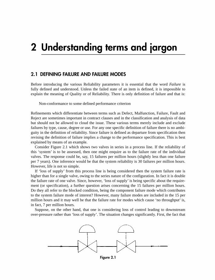
Consider Figure 2.1 which shows two valves in series in a process line. If the reliability ofthis ‘system’ is to be assessed, then one might enquire as to the failure rate of the individualvalves. The response could be, say, 15 failures per million hours (slightly less than one failureper 7 years). One inference would be that the system reliability is 30 failures per million hours.However, life is not so simple.
If ‘loss of supply’ from this process line is being considered then the system failure rate ishigher than for a single valve, owing to the series nature of the configuration. In fact it is doublethe failure rate of one valve. Since, however, ‘loss of supply’ is being specific about the require-ment (or specification), a further question arises concerning the 15 failures per million hours.Do they all refer to the blocked condition, being the component failure mode which contributesto the system failure mode of interest? However, many failure modes are included in the 15 permillion hours and it may well be that the failure rate for modes which cause ‘no throughput’ is,in fact, 7 per million hours.
Suppose, on the other hand, that one is considering loss of control leading to downstreamover-pressure rather than ‘loss of supply’. The situation changes significantly. First, the fact that
Figure 2.1
12 Reliability, Maintainability and Risk
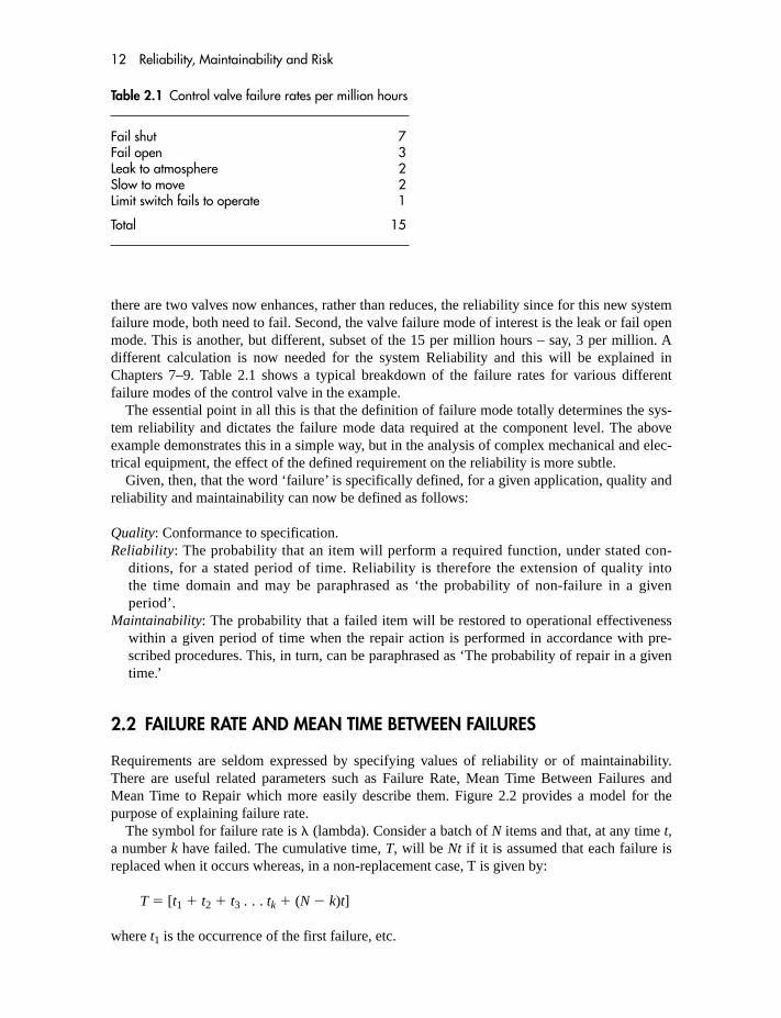
there are two valves now enhances, rather than reduces, the reliability since for this new systemfailure mode, both need to fail. Second, the valve failure mode of interest is the leak or fail openmode. This is another, but different, subset of the 15 per million hours – say, 3 per million. Adifferent calculation is now needed for the system Reliability and this will be explained inChapters 7–9. Table 2.1 shows a typical breakdown of the failure rates for various differentfailure modes of the control valve in the example.
The essential point in all this is that the definition of failure mode totally determines the sys-tem reliability and dictates the failure mode data required at the component level. The aboveexample demonstrates this in a simple way, but in the analysis of complex mechanical and elec-trical equipment, the effect of the defined requirement on the reliability is more subtle.
Given, then, that the word ‘failure’ is specifically defined, for a given application, quality andreliability and maintainability can now be defined as follows:
Quality: Conformance to specification.Reliability: The probability that an item will perform a required function, under stated con-
ditions, for a stated period of time. Reliability is therefore the extension of quality intothe time domain and may be paraphrased as ‘the probability of non-failure in a givenperiod’.
Maintainability: The probability that a failed item will be restored to operational effectivenesswithin a given period of time when the repair action is performed in accordance with pre-scribed procedures. This, in turn, can be paraphrased as ‘The probability of repair in a giventime.’
2.2 FAILURE RATE AND MEAN TIME BETWEEN FAILURES
Requirements are seldom expressed by specifying values of reliability or of maintainability.There are useful related parameters such as Failure Rate, Mean Time Between Failures andMean Time to Repair which more easily describe them. Figure 2.2 provides a model for thepurpose of explaining failure rate.
The symbol for failure rate is � (lambda). Consider a batch of N items and that, at any time t,a number k have failed. The cumulative time, T, will be Nt if it is assumed that each failure isreplaced when it occurs whereas, in a non-replacement case, T is given by:
T � [t1 � t2 � t3 . . . tk � (N � k)t]
where t1 is the occurrence of the first failure, etc.
Table 2.1 Control valve failure rates per million hours
Fail shut 7Fail open 3Leak to atmosphere 2Slow to move 2Limit switch fails to operate 1
Total 15

Understanding terms and jargon 13
2.2.1 The observed failure rate
This is defined: For a stated period in the life of an item, the ratio of the total number of failuresto the total cumulative observed time. If � is the failure rate of the N items then the observed �is given by � k/T. The ^ (hat) symbol is very important since it indicates that k/T is only anestimate of �. The true value will be revealed only when all N items have failed. Making infer-ences about � from values of k and T is the purpose of Chapters 5 and 6. It should also be notedthat the value of is the average over the period in question. The same value could be observedfrom increasing, constant and decreasing failure rates. This is analogous to the case of a motorcar whose speed between two points is calculated as the ratio of distance to time although thevelocity may have varied during this interval. Failure rate is thus only meaningful for situationswhere it is constant.
Failure rate, which has the unit of t�1, is sometimes expressed as a percentage per 1000 hand sometimes as a number multiplied by a negative power of ten. Examples, having the samevalue, are:
8500 per 109 hours (8500 FITS)8.5 per 106 hours or 8.5 � 10�6 per hour0.85 per cent per 1000 hours0.074 per year
Note that these examples each have only two significant figures. It is seldom justified to exceedthis level of accuracy, particularly if failure rates are being used to carry out a reliability predic-tion (see Chapters 8 and 9).
The most commonly used base is per 106 h since, as can be seen in Appendices 3 and 4, itprovides the most convenient range of coefficients from the 0.01 to 0.1 range for microelectron-ics, through the 1–5 range for instrumentation, to the tens and hundreds for larger pieces ofequipment.
The per 109 base, referred to as FITS, is sometimes used for microelectronics where allthe rates are small. The British Telecom database, HRD5, uses this base since it concen-trates on microelectronics and offers somewhat optimistic values compared with othersources.
�
�
Figure 2.2

14 Reliability, Maintainability and Risk
2.2.2 The observed mean time between failures
This is defined: For a stated period in the life of an item, the mean value of the length oftime between consecutive failures, computed as the ratio of the total cumulative observedtime to the total number of failures. If (theta) is the MTBF of the N items then theobserved MTBF is given by � T/k. Once again the hat indicates a point estimate and theforegoing remarks apply. The use of T/k and k /T to define and leads to the inference that� � 1/�.
This equality must be treated with caution since it is inappropriate to compute failure rateunless it is constant. It will be shown, in any case, that the equality is valid only under those cir-cumstances. See Section 2.3, equations (2.5) and (2.6).
2.2.3 The observed mean time to fail
This is defined: For a stated period in the life of an item the ratio of cumulative time to the totalnumber of failures. Again this is T/k. The only difference between MTBF and MTTF is in theirusage. MTTF is applied to items that are not repaired, such as bearings and transistors, andMTBF to items which are repaired. It must be remembered that the time between failuresexcludes the down time. MTBF is therefore mean UP time between failures. In Figure 2.3 it isthe average of the values of (t).
2.2.4 Mean life
This is defined as the mean of the times to failure where each item is allowed to fail. This isoften confused with MTBF and MTTF. It is important to understand the difference. MTBF andMTTF can be calculated over any period as, for example, confined to the constant failure rateportion of the Bathtub Curve. Mean life, on the other hand, must include the failure of everyitem and therefore takes into account the wearout end of the curve. Only for constant failurerate situations are they the same.
To illustrate the difference between MTBF and lifetime compare:
� A match which has a short life but a high MTBF (few fail, thus a great deal of time isclocked up for a number of strikes)
� A plastic knife which has a long life (in terms of wearout) but a poor MTBF (they fail fre-quently)
Again, compare the following:
� The Mean life of human beings is approximately 75 years (this combines random andwearout failures)
� Our MTBF (early to mid-life) is approximately 2500 years (i.e. a 4 � 10�4 pa risk of fatality)
���
�
Figure 2.3

Understanding terms and jargon 15
2.3 INTERRELATIONSHIPS OF TERMS
Returning to the model in Figure 2.2, consider the probability of an item failing in the intervalbetween t and t � dt. This can be described in two ways:
1. The probability of failure in the interval t to t � dt given that it has survived until time twhich is
�(t) dt
where �(t) is the failure rate.
2. The probability of failure in the interval t to t � dt unconditionally, which is
f(t) dt
where f (t) is the failure probability density function.
The probability of survival to time t has already been defined as the reliability, R(t). The ruleof conditional probability therefore dictates that:
Therfore
(2.1)
However, if f (t) is the probability of failure in dt then:
Differentiating both sides:
(2.2)
Substituting equation (2.2) into equation (2.1),
Therefore integrating both sides:
��t
0�(t) dt � �R(t)
1dR(t)/R(t)
��(t) �dR(t)
dt�
1
R(t)
f (t) � � dR(t)
dt
�t
0f (t) dt � probability of failure 0 to t � 1 � R(t)
�(t) �f (t)
R(t)
�(t) dt �f (t) dt
R(t)

A word of explanation concerning the limits of integration is required. �(t) is integratedwith respect to time from 0 to t. 1/R(t) is, however, being integrated with respect to R(t).Now, when t � 0, R(t) � 1 and at t the reliability R(t) is, by definition, R(t). Integratingthen:
But if a � eb then b � loge a, so that:
(2.3)
If failure rate is now assumed to be constant:
(2.4)
Therefore
In order to find the MTBF consider Figure 2.3 again. Let N � K, the number surviving at t,be Ns(t). Then R(t) � Ns(t)/N.
In each interval dt the time accumulated will be Ns(t) dt. At infinity the total will be
Hence the MTBF will be given by:
(2.5)
This is the general expression for MTBF and always holds. In the special case of R(t) � e��t then
(2.6)
Note that inverting failure rate to obtain MTBF, and vice versa, is valid only for the constantfailure rate case.
� �1
�
� � �
0e��t dt
� � �
0R(t) dt
� � �
0
Ns(t) dt
N� �
0R(t) dt
�
0Ns(t) dt
R(t) � e��t
R(t) � exp ���t
0�(t) dt� � exp ��t
t
0
R(t) � exp ���t
0�(t) dt�
� loge R(t)
� loge R(t) � loge1
��t
0�(t) dt � loge R(t)
R(t)
1
16 Reliability, Maintainability and Risk

Understanding terms and jargon 17
2.4 THE BATHTUB DISTRIBUTION
The much-used Bathtub Curve is an example of the practice of treating more than one failuretype by a single classification. It seeks to describe the variation of Failure Rate of componentsduring their life. Figure 2.4 shows this generalized relationship as originally assumed to applyto electronic components. The failures exhibited in the first part of the curve, where failure rateis decreasing, are called early failures or infant mortality failures. The middle portion is referredto as the useful life and it is assumed that failures exhibit a constant failure rate, that is to saythey occur at random. The latter part of the curve describes the wearout failures and it isassumed that failure rate increases as the wearout mechanisms accelerate.
Figure 2.5, on the other hand, is somewhat more realistic in that it shows the Bathtub Curveto be the sum of three separate overlapping failure distributions. Labelling sections of the curveas wearout, burn-in and random can now be seen in a different light. The wearout regionimplies only that wearout failures predominate, namely that such a failure is more likely thanthe other types. The three distributions are described in Table 2.2.
Figure 2.4
Figure 2.5 Bathtub Curve
Failurerate
Earlyfailures Wearout
failures
Time
Useful life
Failurerate
Earlyfailures
Random failures
Wearout
Wearoutfailures
Time
Useful life
Overall curve
Burn-in

18 Reliability, Maintainability and Risk
2.5 DOWN TIME AND REPAIR TIME
It is now necessary to introduce Mean Down Time and Mean Time to Repair (MDT, MTTR).There is frequently confusion between the two and it is important to understand the difference.Down time, or outage, is the period during which equipment is in the failed state. A formal defi-nition is usually avoided, owing to the difficulties of generalizing about a parameter which mayconsist of different elements according to the system and its operating conditions. Consider thefollowing examples which emphasize the problem:
1. A system not in continuous use may develop a fault while it is idle. The fault condition maynot become evident until the system is required for operation. Is down time to be measuredfrom the incidence of the fault, from the start of an alarm condition, or from the time whenthe system would have been required?
2. In some cases it may be economical or essential to leave equipment in a faulty conditionuntil a particular moment or until several similar failures have accrued.
3. Repair may have been completed but it may not be safe to restore the system to its operatingcondition immediately. Alternatively, owing to a cyclic type of situation it may be necessaryto delay. When does down time cease under these circumstances?
It is necessary, as can be seen from the above, to define the down time as required for eachsystem under given operating conditions and maintenance arrangements. MTTR and MDT,although overlapping, are not identical. Down time may commence before repair as in example(1) above. Repair often involves an element of checkout or alignment which may extendbeyond the outage. The definition and use of these terms will depend on whether availability orthe maintenance resources are being considered.
Table 2.2
Known as
Decreasing failure rate Infant mortality Usually related to manufacture and QA, e.g. Burn-in welds, joints, connections, wraps, dirt, impurities, Early failures cracks, insulation or coating flaws, incorrect
adjustment or positioning. In other words, populations of substandard items owing to microscopic flaws.
Constant failure rate Random failures Usually assumed to be stress-related failures. That Useful life is, random fluctuations (transients) of stress Stress-related failures exceeding the component strength Stochastic failures (see Chapter 11). The design reliability referred to
in Figure 1.1 is of this type.
Increasing failure rate Wearout failures Owing to corrosion, oxidation, breakdown of insulation, atomic migration, friction wear, shrinkage, fatigue, etc.

Understanding terms and jargon 19
The significance of these terms is not always the same, depending upon whether a system, areplicated unit or a replaceable module is being considered.
Figure 2.6 shows the elements of down time and repair time:
(a) Realization Time: This is the time which elapses before the fault condition becomesapparent. This element is pertinent to availability but does not constitute part of therepair time.
(b) Access Time: This involves the time, from realization that a fault exists, to make contactwith displays and test points and so commence fault finding. This does not include travelbut the removal of covers and shields and the connection of test equipment. This is deter-mined largely by mechanical design.
(c) Diagnosis Time: This is referred to as fault finding and includes adjustment of test equip-ment (e.g. setting up a lap top or a generator), carrying out checks (e.g. examining wave-forms for comparison with a handbook), interpretation of information gained (this may beaided by algorithms), verifying the conclusions drawn and deciding upon the correctiveaction.
(d) Spare part procurement: Part procurement can be from the ‘tool box’, by cannibalization orby taking a redundant identical assembly from some other part of the system. The timetaken to move parts from a depot or store to the system is not included, being part of thelogistic time.
(e) Replacement Time: This involves removal of the faulty LRA (Least Replaceable Assembly)followed by connection and wiring, as appropriate, of a replacement. The LRA is thereplaceable item beyond which fault diagnosis does not continue. Replacement time islargely dependent on the choice of LRA and on mechanical design features such as thechoice of connectors.
Figure 2.6 Elements of down time and repair time
20 Reliability, Maintainability and Risk
(f) Checkout Time: This involves verifying that the fault condition no longer exists and that thesystem is operational. It may be possible to restore the system to operation before complet-ing the checkout in which case, although a repair activity, it does not all constitute downtime.
(g) Alignment Time: As a result of inserting a new module into the system, adjustments may berequired. As in the case of checkout, some or all of the alignment may fall outside the downtime.
(h) Logistic Time: This is the time consumed waiting for spares, test gear, additional tools andmanpower to be transported to the system.
(i) Administrative Time: This is a function of the system user’s organization. Typical activitiesinvolve failure reporting (where this affects down time), allocation of repair tasks, man-power changeover due to demarcation arrangements, official breaks, disputes, etc.
Activities (b)–(g) are called Active Repair Elements and (h) and (i) Passive Repair Activities.Realization time is not a repair activity but may be included in the MTTR where down time isthe consideration. Checkout and alignment, although utilizing manpower, can fall outside thedown time. The Active Repair Elements are determined by design, maintenance arrangements,environment, manpower, instructions, tools and test equipment. Logistic and Administrativetime is mainly determined by the maintenance environment, that is, the location of spares,equipment and manpower and the procedure for allocating tasks.
Another parameter related to outage is Repair rate (�). It is simply the down time expressedas a rate, therefore:
� � 1/MTTR
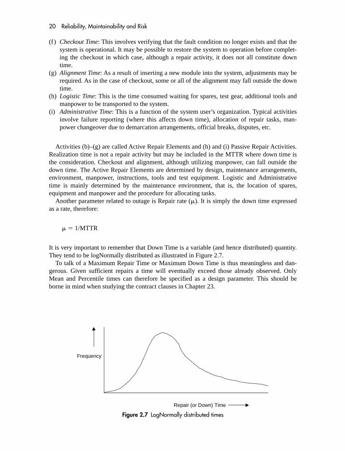
It is very important to remember that Down Time is a variable (and hence distributed) quantity.They tend to be logNormally distributed as illustrated in Figure 2.7.
To talk of a Maximum Repair Time or Maximum Down Time is thus meaningless and dan-gerous. Given sufficient repairs a time will eventually exceed those already observed. OnlyMean and Percentile times can therefore be specified as a design parameter. This should beborne in mind when studying the contract clauses in Chapter 23.
Frequency
Repair (or Down) Time
Figure 2.7 LogNormally distributed times

Understanding terms and jargon 21
2.6 AVAILABILITY, UNAVAILABILITY AND PROBABILITY OF FAILUREON DEMAND
In Chapter 1, Availability was introduced as a useful parameter which describes theamount of available time. It is determined by both the reliability and the maintainability ofthe item. Returning to Figure 2.3 it is the ratio of the (t) values to the total time. Availabilityis, therefore:
This is known as the steady-state availability and can be expressed as a ratio or as a percentage.Usually it is more convenient to use Unavailability which is the same thing as the Probability ofFailure on Demand (PFD):
In the case of unrevealed failures the down time is equal to half the proof-test interval, T (plusthe actual MTTR). This can be illustrated by thinking about an annual proof-test interval for themotor car. Consider the unrevealed failure of the air bag which occurs, at random, during theyear. If we collect data for enough failures some will have occurred early in the year, some latein the year, and some at other times. The average of the times will be the middle which is T/2.This is developed further in Chapter 8.
Thus the Unavailability becomes � MDT � � T/2.
2.7 HAZARD AND RISK-RELATED TERMS
Failure rate and MTBF terms, such as have been dealt with in this chapter, are equally applica-ble to hazardous failures. Hazard is usually used to describe a situation with the potential forinjury or fatality whereas failure is the actual event, be it hazardous or otherwise. The termmajor hazard is different only in degree and refers to certain large-scale potential incidents.These are dealt with in Chapters 10, 21 and 22.
Risk is a term which actually covers two parameters. The first is the probability (or rate) of aparticular event. The second is the scale of consequence (perhaps expressed in terms of fatali-ties). This is dealt with in Chapter 10. Terms such as societal and individual risk differentiatebetween failures which cause either multiple or single fatalities.
A � 1 � A �� MDT
1 � � MDT� � MDT
�MTBF
MTBF � MDT
�Average of (t)
Average of (t) � Mean down time
�Up time
Up time � Down time
A �Up time
Total time

22 Reliability, Maintainability and Risk
2.8 CHOOSING THE APPROPRIATE PARAMETER
It is clear that there are several parameters available for describing the reliability and maintain-ability characteristics of an item. In any particular instance there is likely to be one parametermore appropriate than the others. Although there are no hard-and-fast rules the following guide-lines may be of some assistance:
Failure Rate: Applicable to most component parts. Useful at the system level, whenever con-stant failure rate applies, because it is easy to compute Unavailability from � � MDT.Remember, however, that failure rate is meaningless if it is not constant. The failure distribu-tion would then be described by other means which will be explained in Chapter 6.
MTBF and MTTF: Often used to describe equipment or system reliability. Of use when calcu-lating maintenance costs. Meaningful even if the failure rate is not constant.
Reliability/Unreliability: Used where the probability of failure is of interest as, for example, inaircraft landings where safety is the prime consideration.
Maintainability: Seldom used as such.Mean Time To Repair: Often expressed in percentile terms such as the 95 percentile repair time
shall be 1 hour. This means that only 5% of the repair actions shall exceed 1 hour. MaximumMTTRs are meaningless.
Mean Down Time: Used where the outage affects system reliability or availability. Oftenexpressed in percentile terms. Maximum MDTs are meaningless.
Availability/Unavailability: Very useful where the cost of lost revenue, owing to outage, is ofinterest. Combines reliability and maintainability. Ideal for describing process plant.Unavailability calculates the probability of failure on demand (PFD) commonly needed as atarget for safety-related systems.
Mean Life: Beware of the confusion between MTTF and Mean Life. Whereas the Mean Lifedescribes the average life of an item taking into account wearout, the MTTF is the averagetime between failures. The difference is clear if one considers the simple example of thematch.
There are sources of standard definitions such as:
BS 4778: Part 3.2BS 4200: Part 1IEC Publication 271US MIL STD 721BUK Defence Standard 00-5 (Part 1)Nomenclature for Hazard and Risk in the Process Industries (I Chem E)IEC 61508 (Part 4)
It is, however, not always desirable to use standard sources of definitions so as to avoid specify-ing the terms which are needed in a specification or contract. It is all too easy to ‘define’ theterms by calling up one of the aforementioned standards. It is far more important that terms arefully understood before they are used and if this is achieved by defining them for specific situa-tions, then so much the better. The danger in specifying that all terms shall be defined by agiven published standard is that each person assumes that he or she knows the meaning of eachterm and these are not read or discussed until a dispute arises. The most important area involv-ing definition of terms is that of contractual involvement where mutual agreement as to themeaning of terms is essential. Chapter 19 will emphasize the dangers of ambiguity.

Understanding terms and jargon 23
Useful notes1. If failure rate is constant and, hence , then after one MTBF the probability of survival, R(t) is e�1,
which is 0.37.2. If t is small, approaches 1 � �t. For example, if � � 10�5 and t � 10 then approaches 1 � 10�4 �
0.9999.
3. Since � � R(t) dt, it is useful to remember that .
EXERCISES
If � � (a) 1 � 10�6 per hr (b) 100 � 10�6 per hr
1. Calculate the MTBFs in years.2. Calculate the Reliability for 1 year (R(1yr)).3. If the MDT is 10 hrs, calculate the Unavailability.4. If the MTTR is 1 hour, the failures are dormant, and the inspection interval is 6 months, cal-
culate the Unavailability.5. What is the effect of doubling the MTTR?6. What is the effect of doubling the inspection interval?
�
0 Ae�B�t � (A/B�)�
0
e��te��t
R � e��t � e�t/�

3 A cost-effective approachto quality, reliability and safety
3.1 RELIABILITY AND COST
So far, only manufacturers’ quality costs have been discussed. The costs associated with acquiring,operating and maintaining equipment are equally relevant to a study such as ours. The total costsincurred over the period of ownership of equipment are often referred to as Life-Cycle Costs. Thesecan be separated into:
Acquisition Cost – Capital cost plus cost of installation, transport, etc.Ownership Cost – Cost of preventive and corrective maintenance and of modifications.Operating Cost – Cost of materials and energy.Administration Cost – Cost of data acquisition and recording and of documentation.
They will be influenced by:
Reliability – Determines frequency of repair.Fixes spares requirements.Determines loss of revenue (together with maintainability).
Maintainability – Affects training, test equipment, down time, manpower.Safety Factors – Affect operating efficiency and maintainability.
Life-cycle costs will clearly be reduced by enhanced reliability, maintainability and safetybut will be increased by the activities required to achieve them. Once again the need to findan optimum set of parameters which minimizes the total cost is indicated. This concept isillustrated in Figures 3.1 and 3.2. Each curve represents cost against Availability. Figure 3.1shows the general relationship between availability and cost. The manufacturer’s pre-deliverycosts, those of design, procurement and manufacture, increase with availability. On the otherhand, the manufacturer’s after-delivery costs, those of warranty, redesign, loss of reputation,decrease as availability improves. The total cost is shown by a curve indicating some value ofavailability at which minimum cost is incurred. Price will be related to this cost. Taking, then,the price/availability curve and plotting it again in Figure 3.2, the user’s costs involve theaddition of another curve representing losses and expense, owing to failure, borne by theuser. The result is a curve also showing an optimum availability which incurs minimum cost.Such diagrams serve only to illustrate the philosophy whereby cost is minimized as a resultof seeking reliability and maintainability enhancements whose savings exceed the initialexpenditure.

A cost-effective approach to quality, reliability and safety 25
A typical application of this principle is as follows:
� A duplicated process control system has a spurious shutdown failure rate of 1 per annum.� Triplication reduces this failure rate to 0.8 per annum.� The Mean Down Time, in the event of a spurious failure, is 24 hours.� The total cost of design and procurement for the additional unit is £60 000.� The cost of spares, preventive maintenance, weight and power arising from the additional
unit is £1000 per annum.� The continuous process throughput, governed by the control system, is £5 million per annum.� The potential saving is (1 � 0.8) � 1/365 � £5 million per annum � £2740 per annum
which is equivalent to a capital investment of, say, £30 000.� The cost is £60 000 plus £1000 per annum which is equivalent to a capital investment of,
say, £70 000.
Costsafterdelivery
Costsbeforedelivery
Man
ufac
ture
r’s c
osts
Total
Availability
Figure 3.1 Availability and cost – manufacturer
Availability
Costs offailure
Price
Total
Use
r’s c
osts
Figure 3.2 Availability and cost – user

26 Reliability, Maintainability and Risk
There may be many factors influencing the decision such as safety, weight, space available,etc. From the reliability cost point of view, however, the expenditure is not justified.
The cost of carrying out RAMS-cycle predictions will usually be small compared with thepotential safety or life-cycle cost savings as shown in the following examples.
A cost justification may be requested for carrying out these RAMS prediction activities. Inwhich case the costs of the following activities should be estimated, for comparison with thepredicted savings. RAMS prediction costs (i.e. resources) will depend upon the complexity ofthe equipment. The following two budgetary examples, expressing RAMS prediction costs as apercentage of the total development and procurement costs, are given:
Example (A) A simple safety subsystem consisting of a duplicated ‘shut down’ or ‘firedetection’ system with up to 100 inputs and outputs, including power supplies, annunciationand operator interfaces.
Example (B) A single stream plant process (e.g. chain of gas compression, chain of H2Sremoval reactors and vessels) and associated pumps and valves (up to 20) and the associatedinstrumentation (up to 50 pressure, flow and temperature transmitters).
Man-days Man-daysfor (A) for (B)
Figure 1.2 loop [1]: Feasibility RAMS prediction. This will 4 6consist of a simple block diagram prediction with thevessels or electronic controllers treated as units.
Figure 1.2 loop [2]: Conceptual design prediction. Similar to [1] 10 13but with more precise input/output quantities.
Figure 1.2 loop [3]: Detailed design prediction. Includes Failure 6 18Modes, Effects and Criticality Analysis Module (FMECA) at circuit level for 75% of the units, attention to common cause,human error and proof-test intervals.
Figure 1.2 loop [4]: RAMS testing. This refers to preparing 2 10subsystem and system test plans and analysis of test data ratherthan the actual test effort.
Figure 1.2 loop [5]: Acceptance testing. This refers to preparing 2 6test plans and analysis of test data rather than the actual test effort.
Figure 1.2 loop [6]: First year, reliability growth reviews. This is 1 2a form of design review using field data.
Figure 1.2 loop [7]: Subsequent reliability growth, data analysis. 2 3
Figure 1.2 loop [9]: First year, field data analysis. Not including 2 8effort for field data recording but analysis of field returns.
Figure 1.2 loop [10]: RCM planning. This includes identification 3 8of major components, establishing RAMS data for them,calculation of optimum discard, spares and proof-test intervals.

A cost-effective approach to quality, reliability and safety 27
Man-days for (A) Man-days for (B)
Overall totals 32 74Cost @ £250/man-day £8K £18.5KTypical project cost (design and Procure) £150K £600KRAMS cost as % of Total Project Cost 5.3% 3.1%
Life-cycle costs (for both safety and unavailability) can be orders greater than the above quotedproject costs. Thus, even relatively small enhancements in MTBF/Availability will easily lead tocosts far in excess of the example expenditures quoted above.
The cost of carrying out RAMS prediction activities is in the order of 3% to 5% of total projectcost. Although definitive records are not readily available it is credible that the assessmentprocess, with its associated comparison of alternatives and proposed modifications, will lead tosavings which exceed this outlay. In the above examples, credible results of the RAMS studiesmight be:
(A) ESD system:The unavailability might typically be improved from 0.001 to 0.0005 as a result of the RAMstudy. Spurious shutdown, resulting from failure of the ESD, might typically be £500 000 perday for a small gas production platform. Thus, the £8000 expenditure on RAM saves:
£500 000 � (0.001 � 0.0005) � 365 � £91 000 per annum
(B) H2S system:The availability might typically be improved from 0.95 to 0.98 as a result of the RAMstudy. Loss of throughput, resulting from failure, might typically cost £5000 per day. Thus,the £18 500 expenditure on RAM saves:
£5000 � (0.98 � 0.95) � 365 � £55 000 per annum
Non RAMS-specialist engineers should receive training in RAMS techniques in orderthat they acquire sufficient competence to understand the benefits of those activities. TheIEE/BCS competency guidelines document 1999, offers a framework for assessing suchcompetencies.
3.2 COSTS AND SAFETY
3.2.1 The need for optimization
Once the probability of a hazardous event has been assessed, the cost of the various measureswhich can be taken to reduce that risk is inevitably considered. If the risk to life is so high that itmust be reduced as a matter of priority, or if the measures involved are a legal requirement, then theeconomics are of little or no concern – the equipment or plant must be made safe or closed down.
If, however, the risk to life is perceived to be sufficiently low then the reduction inrisk for a given expenditure can be examined to see if the expenditure can be justified.

28 Reliability, Maintainability and Risk
At this point the concept of ALARP (As Low As Reasonably Practicable) becomes relevantin order that resources are allocated in the most effective manner. Risk has been defined asbeing ALARP if the reduction in risk is insignificant in relation to the cost of avertingthat risk. The problem here is that the words ‘insignificant’ and ‘not worth the cost’ are notquantifiably defined.
One approach is to consider the risks which society considers to be acceptable for bothvoluntary and involuntary situations. This is addressed in the Health and Safety Executivepublications, The Tolerability of Risk from Nuclear Power Installations and Reducing RisksProtecting People, as well as some other publications in this area. This topic is developed inSection 10.2 of Chapter 10.
3.2.2 Cost per life saved
A controversial parameter is the Cost per Life Saved. This has a value in the ranking of possibleexpenditures so as to apply funds to the most effective area of risk improvement. Any techniquewhich appears to put a price on human life is, however, potentially distasteful and thus attemptsto use it are often resisted. It should not, in any case, be used as the sole criterion for decidingupon expenditure.
The concept is illustrated by the following hypothetical examples:
1. A potential improvement to a motor car braking system is costed at £40. Currently, the numberof fatalities per annum in the UK is in the order of 3000. It is predicted that 500 lives per annummight be saved by the design. Given that 2 million cars are manufactured each year then the costper life saved is calculated as:
2. A major hazard process is thought to have an annual frequency of 10�6 for a release whoseconsequences are estimated to be 80 fatalities. An expenditure of £150 000 on new controlequipment is predicted to improve this frequency to 0.8 � 10�6. The cost per life saved,assuming a 40-year plant life, is thus:
The examples highlight the difference in acceptability between individual and societal risk.Many would prefer the expenditure on the major plant despite the fact that the vehicle proposalrepresents more lives saved per given expenditure. Naturally, such a comparison in cost per lifesaved terms would not be made, but the method has validity when comparing alternativeapproaches to similar situations.
The question arises as to the value of ‘cost per life saved’ to be used. Organizations arereluctant to state grossly disproportionate levels of CPL. Currently, figures in the range of£500 000 to £2 000 000 are common. Where a risk has the potential for multiple fatalitiesthen higher sums may be used.
However, a value must be chosen, by the plant operator, for each assessment. The valueselected must take account of any uncertainty inherent in the assessment and may have to
£150 000
80 � (10�6 � 0.8 � 10�6) � 40� £230 million
£40 � 2 million
500� £160 000

A cost-effective approach to quality, reliability and safety 29
take account of any company specific issues such as the number of similar installations.The greater the potential number of lives lost and the greater the aversion to the scenariothen the larger is the choice of the cost per life saved criteria. Values which have beenquoted include:
1. Approximately £1 000 000 by HSE, 1999 where there is a recognized scenario, a voluntaryaspect to the exposure, a sense of having personal control, small numbers of casualties perincident. An example would be PASSENGER ROAD TRANSPORT.
2. Approximately £2 000 000–£4 000 000 by the HSE, 1991 where the risk is not underpersonal control and therefore an involuntary risk. An example would be TRANSPORTOF DANGEROUS GOODS.
3. Approximately £5 000 000–£15 000 000, mooted in the press, where there are large numbersof fatalities, there is uncertainty as to the frequency and no personal control by the victim. Anexample would be MULTIPLE RAIL PASSENGER FATALITIES.
4. This is a controversial area and figures can be subject to rapid revision in the light ofcatastrophic incidents and subsequent media publicity. A recent example, of the demand forautomatic train protection in the UK, involves approximately £14 000 000 per life saved. Thisis despite the earlier rail industry practice of regarding £2 000 000 as an appropriate figure.
In many assessments, no specific risk reduction measure has yet been proposed and thus nocost is known. However, the calculation can be used, rather than to calculate the CPL, tocalculate the cost which should be contemplated, given some CPL criteria. Thus:
The frequency of some hazardous failure maps to a risk of 6.5 � 10�6 pa. It is less than the‘Maximum Tolerable Risk’ but not small enough to be considered ‘Broadly Acceptable’ andis therefore in the ALARP region.
If a cost per life saved criteria of £4 000 000 is used then the expenditure on any proposalwhich might reduce the risk to 10�6 pa can be calculated (assuming 2 fatalities and a 30-yearplant life) as:
£4 000 000 � £proposed/([6.5 � 10�6 � 1 � 10�6] � 2 � 30)
Thus £proposed � 1320
Any proposal involving less than £1320 which would reduce the risk to 10�6 pa should beconsidered. This might well be possible if proof-test intervals are reduced.
This provides a useful way of indicating whether risk reduction is or is not feasible within thecost indicated.
3.2.3 Costs and savings involved with safety
Although costs vary considerably, according to the scale and complexity of a system orproject, the following typical resources have been seen in meeting various aspects ofsafety-integrity.
Typical safety-integrity targeting with random hardware failures predictions and thedemonstration of ALARP – 2 to 6 man-days.
30 Reliability, Maintainability and Risk
Assessing safe failure fraction (described in Chapter 22) – 1 to 5 man-days.
Bringing an ISO 9000 management system up to IEC 61508 functional safety capability –5 man-days for the purpose of a product demonstration, 20 to 50 man-days for the purposeof accredited certification.
As far as savings are concerned:
There is an intangible but definite benefit due to enhanced credibility in themarket place. Additional sales vis-à-vis those who have not demonstrated integrityare likely.
Major savings are purported to be in reduced maintenance for those (often the majority)systems for which it can be demonstrated that low-integrity targets are adequate (Chapter 22).This also has the affect of focusing effort onto those systems with higher-integrity targets.
Conversely, there are penalty costs associated with hazardous failures:
The manufacturer and the user will be involved in far higher costs of retrospective redesignif subsequent changes are needed to meet the maximum tolerable risk.
The user could face enormous legal costs in the event of a major incident which invokesthe H&SW Act (Chapter 20), especially if appropriate functional safety standards have notbeen addressed when it is reasonably practicable to do so.
3.3 THE COST OF QUALITY
The practice of identifying quality costs is not new, although it is only very large organizationsthat collect and analyse this highly significant proportion of their turnover. Attempts to setbudget levels for the various elements of quality costs are even rarer. This is unfortunate, sincethe contribution of any activity to a business is measured ultimately in financial terms and theactivities of quality, reliability and maintainability are no exception. If the costs of failure andrepair were more fully reported and compared with the costs of improvement then greaterstrides would be made in this branch of engineering management. Greater recognition leads tothe allocation of more resources. The pursuit of quality and reliability for their own sake is nojustification for the investment of labour, plant and materials.
Quality Cost analysis entails extracting various items from the accounts and grouping themunder three headings:
Prevention Costs – costs of preventing failures.Appraisal Costs – costs related to measurement.Failure Costs – costs incurred as a result of scrap, rework, failure, etc.
Each of these categories can be broken down into identifiable items and Table 3.1 shows a typicalbreakdown of quality costs for a six-month period in a manufacturing organization. The totals areexpressed as a percentage of sales, this being the usual ratio. It is known by those who collect

A cost-effective approach to quality, reliability and safety 31
these costs that they are usually under-recorded and that the failure costs obtained can be as littleas a quarter of the true value. The ratios shown in Table 3.1 are typical of a manufacturing andassembly operation involving light machining, assembly, wiring and functional test of electricalequipment. The items are as follows:
Prevention Costs
Design Review – Review of new designs prior to the release of drawings.Quality and Reliability Training – Training of QA staff. Q and R Training of other staff.Vendor Quality Planning – Evaluation of vendors’ abilities to meet requirements.Audits – Audits of systems, products, processes.Installation Prevention Activities – Any of these activities applied to installations and the
commissioning activity.Product Qualification – Comprehensive testing of a product against all its specifications prior
to the release of final drawings to production. Some argue that this is an appraisal cost. Sinceit is prior to the main manufacturing cycle the author prefers to include it in Prevention sinceit always attracts savings far in excess of the costs incurred.
Quality Engineering – Preparation of quality plans, workmanship standards, inspection procedures.
Table 3.1 Quality costs: 1 January 2000 to 30 June 2000 (sales £2 million)
Prevention Costs £’000 % of SalesDesign review 0.5Quality and reliability training 2Vendor quality planning 2.1Audits 2.4Installation prevention activities 3.8Product qualification 3.5Quality engineering 3.8
18.1 0.91
Appraisal CostsTest and inspection 45.3Maintenance and calibration 2Test equipment depreciation 10.1Line quality engineering 3.6Installation testing 5
66.0 3.3
Failure CostsDesign changes 18Vendor rejects 1.5Rework 20Scrap and material renovation 6.3Warranty 10.3Commissioning failures 5Fault finding in test 26
87.1 4.36
Total quality cost 171.2 8.57

32 Reliability, Maintainability and Risk
Appraisal Costs
Test and Inspection – All line inspection and test activities excluding rework and waiting time.If the inspectors or test engineers are direct employees then the costs should be suitably loaded.It will be necessary to obtain, from the cost accountant, a suitable overhead rate which allowsfor the fact that the QA overheads are already reported elsewhere in the quality cost report.
Maintenance and Calibration – The cost of labour and subcontract charges for the calibration,overhaul, upkeep and repair of test and inspection equipment.
Test Equipment Depreciation – Include all test and measuring instruments.Line Quality Engineering – That portion of quality engineering which is related to answering
test and inspection queries.Installation Testing – Test during installation and commissioning.
Failure Costs
Design Changes – All costs associated with engineering changes due to defect feedback.Vendor Rejects – Rework or disposal costs of defective purchased items where this is not
recoverable from the vendor.Rework – Loaded cost of rework in production and, if applicable, test.Scrap and Material Renovation – Cost of scrap less any reclaim value. Cost of rework of any
items not covered above.Warranty – Warranty: labour and parts as applicable. Cost of inspection and investigations to be
included.Commissioning Failures – Rework and spares resulting from defects found and corrected during
installation.Fault Finding in Test – Where test personnel carry out diagnosis over and above simple
module replacement then this should be separated out from test and included in this item.In the case of diagnosis being carried out by separate repair operators then that should beincluded.
A study of the above list shows that reliability and maintainability are directly related to theseitems.
UK industry turnover is in the order of £150 thousand million. The total quality cost fora business is likely to fall between 4% and 15%, the average being somewhere in the regionof 8%. Failure costs are usually approximately 50% of the total – higher if insufficient isbeing spent on prevention. It is likely then that about £6 thousand million was wasted indefects and failures. A 10% improvement in failure costs would release into the economyapproximately
£600 million
Prevention costs are likely to be approximately 1% of the total and therefore thousandmillion.
In order to introduce a quality cost system it is necessary to:
Convince top management – Initially a quality cost report similar to Table 3.1 should be prepared.The accounting system may not be arranged for the automatic collection and grouping of theitems but this can be carried out on a one-off basis. The object of the exercise is to demonstratethe magnitude of quality costs and to show that prevention costs are small by comparison withthe total.
£112

A cost-effective approach to quality, reliability and safety 33
Collect and Analyse Quality Costs – The data should be drawn from the existing accountingsystem and no major change should be made. In the case of change notes and scrappeditems, the effort required to analyse every one may be prohibitive. In this case the totalmay be estimated from a representative sample. It should be remembered, whenanalysing change notes, that some may involve a cost saving as well as an expenditure. Itis the algebraic total which is required.
Quality Cost Improvements – The third stage is to set budget values for each of the qualitycost headings. Cost-improvement targets are then set to bring the larger items down to anacceptable level. This entails making plans to eliminate the major causes of failure.Those remedies which are likely to realize the greatest reduction in failure cost for thesmallest outlay should be chosen first.
Things to remember about Quality Costs are:
� They are not a target for individuals but for the company.� They do not provide a comparison between departments because quality costs are rarely
incurred where they are caused.� They are not an absolute financial measure but provide a standard against which to make
comparisons. Consistency in their presentation is the prime consideration.

This Page is Intentionally Left Blank

Part TwoInterpreting Failure Rates

This Page is Intentionally Left Blank

4 Realistic failure ratesand prediction confidence
4.1 DATA ACCURACY
There are many collections of failure rate data compiled by defence, telecommunications,process industries, oil and gas and other organizations. Some are published data Handbookssuch as:
US MIL HANDBOOK 217 (Electronics)CNET (French PTT) DataHRD (Electronics, British Telecom)RADC Non-Electronic Parts Handbook NPRDOREDA (Offshore data)FARADIP.THREE (Data ranges)
Some are data banks which are accessible by virtue of membership or fee such as:
SRD (Systems Reliability Department of UKAEA) Data BankTechnis [the author] (Tonbridge)
Some are in-house data collections which are not generally available. These occur in:
Large industrial manufacturersPublic utilities
These data collection activities were at their peak in the 1980s but, sadly, they declined duringthe 1990s and the majority of published sources have not been updated since that time.
Failure data are usually, unless otherwise specified, taken to refer to random failures (i.e.constant failure rates). It is important to read, carefully, any covering notes since, for a giventemperature and environment, a stated component, despite the same description, may exhibit awide range of failure rates because:
1. Some failure rate data include items replaced during preventive maintenance whereas othersdo not. These items should, ideally, be excluded from the data but, in practice, it is notalways possible to identify them. This can affect rates by an order of magnitude.
2. Failure rates are affected by the tolerance of a design and this will cause a variation in thevalues. Because definitions of failure vary, a given parametric drift may be included in onedatabase as a failure, but ignored in another.

38 Reliability, Maintainability and Risk
3. Although nominal environmental and quality assurance levels are described in some databases,the range of parameters covered by these broad descriptions is large. They represent, therefore,another source of variability.
4. Component parts often are only described by reference to their broad type (e.g. signaltransformer). Data are therefore combined for a range of similar devices rather than beingseparately grouped, thus widening the range of values. Furthermore, different failure modesare often mixed together in the data.
5. The degree of data screening will affect the relative numbers of intrinsic and induced failuresin the quoted failure rate.
6. Reliability growth occurs where field experience is used to enhance reliability as a result ofmodifications. This will influence the failure rate data.
7. Trial and error replacement is sometimes used as a means of diagnosis and this can artificiallyinflate failure rate data.
8. Some data records undiagnosed incidents and ‘no fault found’ visits. If these are included inthe statistics as faults, then failure rates can be inflated. Quoted failure rates are thereforeinfluenced by the way they are interpreted by an analyst.
Failure rate values can span one or two orders of magnitude as a result of different combina-tions of these factors. Prediction calculations are explained in Chapters 8 and 9 and it will beseen (Section 4.4) that the relevance of failure rate data is more important than refinements inthe statistics of the calculation. The data sources described in Section 4.2 can at least be sub-divided into ‘Site specific’, ‘Industry specific’ and ‘Generic’ and the work described inSection 4.4 will show that the more specific the data source the greater the confidence in theprediction.
Failure rates are often tabulated, for a given component type, against ambient temperature andthe ratio of applied to rated stress (power or voltage). Data is presented in one of two forms:
1. Tables: Lists of failure rates such as those in Appendices 3 and 4, with or without multiplyingfactors, for such parameters as quality and environment.
2. Models: Obtained by regression analysis of the data. These are presented in the form ofequations which yield a failure rate as a result of inserting the device parameters into theappropriate expression.
Because of the large number of variables involved in describing microelectronic devices,data are often expressed in the form of models. These regression equations (WHICH GIVEA TOTALLY MISLEADING IMPRESSION OF PRECISION) involve some or all of thefollowing:
� Complexity (number of gates, bits, equivalent number of transistors).� Number of pins.� Junction temperature (see Arrhenius, Section 11.2).� Package (ceramic and plastic packages).� Technology (CMOS, NMOS, bipolar, etc.).� Type (memory, random LSI, analogue, etc.).� Voltage or power loading.� Quality level (affected by screening and burn-in).� Environment.� Length of time in manufacture.

Realistic failure rates and prediction confidence 39
Although empirical relationships have been established relating certain device failure ratesto specific stresses, such as voltage and temperature, no precise formula exists which linksspecific environments to failure rates. The permutation of different values of environmentalfactors, such as those listed in Chapter 12, is immense. General adjustment (multiplying) fac-tors have been evolved and these are often used to scale up basic failure rates to particularenvironmental conditions.
Because Failure Rate is, probably, the least precise engineering parameter, it is important tobear in mind the limitations of a Reliability prediction. The work described in Section 4.4 nowmakes it possible to express predictions using confidence intervals. The resulting MTBF,Availability (or whatever) should not be taken as an absolute parameter but rather as a generalguide to the design reliability. Within the prediction, however, the relative percentages of contri-bution to the total failure rate are of a better accuracy and provide a valuable tool in designanalysis.
Because of the differences between data sources, comparisons of reliability should alwaysinvolve the same data source in each prediction.
For any reliability assessment to be meaningful, it must address a specific system failuremode. To predict that a safety (shutdown) system will fail at a rate of, say, once per annum is,on its own, saying very little. It might be that 90% of the failures lead to a spurious shutdownand 10% to a failure to respond. If, on the other hand, the ratios were to be reversed then thepicture would be quite different.
The failure rates, mean times between failures or availabilities must therefore be assessed fordefined failure types (modes). In order to achieve this, the appropriate component level failuremodes must be applied to the prediction models which are described in Chapters 8 and 9.Component failure mode data is sparse but a few of the sources do contain some information.The following sections indicate where this is the case.
4.2 SOURCES OF DATA
Sources of failure rate and failure mode data can be classified as:
1. SITE/COMPANY SPECIFIC:Failure rate data which have been collected from similar equipment being used on very simi-lar sites (e.g. two or more gas compression sites where environment, operating methods,maintenance strategy and equipment are largely the same). Another example would be theuse of failure rate data from a flow corrector used throughout a specific distribution network.This data might be applied to the RAMS prediction for a new design of circuitry for thesame application.
2. INDUSTRY SPECIFIC:An example would be the use of the OREDA offshore failure rate data book for a RAMSprediction of a proposed offshore process package.
3. GENERIC:A generic data source combines a large number of applications and sources.
As will be emphasized in Chapters 7–9, predictions require failure rates for specific modes offailure (e.g. open circuit, signal high, valve closes). Some, but unfortunately only a few, datasources contain specific failure mode percentages. Mean time to repair data is even more sparsealthough the OREDA database is very informative in this respect.

40 Reliability, Maintainability and Risk
The following are the more widely used sources:
4.2.1 Electronic failure rates
4.2.1.1 US Military Handbook 217 (Generic, no failure modes)This is one of the better known data sources and is from RADC (Rome Air Data Centre in theUSA). Opinions are sharply divided as to its value due to the unjustified precision implied byvirtue of its regression model nature of its microelectronics sections. It covers:
MicroelectronicsDiscrete semiconductorsTubes (thermionic)LasersResistors and capacitorsInductorsConnections and connectorsMetersCrystalsLamps, fuses and other miscellaneous items
The Microelectronics sections present the information as a number of regression models. Forexample, the Monolithic Bipolar and MOS Linear Device model is given as:
Part operating failure rate model ( ):
where
is a multiplier for quality,is a multiplier for junction temperature,is a multiplier for applied voltage stress,is an application multiplier for environment,is a multiplier for the amount of time the device has been in production,
C1 is based on the equivalent transistor count in the device,C2 is related to the packaging.
There are two reservations about this approach. First, it is not possible to establish the originalapplication of the items from which the data are derived and it is not clear what mix of field andtest data pertains. Second, a regression model both interpolates and extrapolates the results of rawdata. There are similar models for other microelectronic devices and for discrete semiconductors.Passive components are described using tables of failure rates and the use of multipliers to takeaccount of Quality and Environment.
The trend in successive issues of MIL-217 has been towards lower failure rates, particularlyin the case of microelectronics. This is also seen in other data banks and may reflect the steadyincrease in manufacturing quality and screening techniques over the last 15 years. On the otherhand, it may be due to reassessing the earlier data. MIL-217 is available (as MILSTRESS) ondisk from ITEM software. Between 1965 and 1991, it moved from Issue A to Issue F (amended1992). It seems unlikely that it will be updated again.
�L
�E
�V
�t
�Q
�p � �Q (C1�t�V � C2�E)�L Failures/106 hours
�p

Realistic failure rates and prediction confidence 41
4.2.1.2 HRD5 Handbook of Reliability Data for Electronic Components Usedin Telecommunications Systems (Industry specific, no failure modes)This document was produced, from field data, by British Telecom’s Laboratories at MartleshamHeath and offers failure rate lists for Integrated Circuits, Discrete Semiconductors, Capacitors,Resistors, Electromechanical and Wound Components, Optoelectronics, Surge Protection,Switches, Visual Devices and a Miscellaneous section (e.g. microwave).
The failure rates obtained from this document are generally optimistic compared with theother sources, often by as much as an order of magnitude. This is due to an extensive ‘screen-ing’ of the data whereby failures which can be attributed to a specific cause are eliminatedfrom the data once remedial action has been introduced into the manufacturing process.Considerable effort is also directed towards eliminating maintenance-induced failures fromthe data.
Between 1977 and 1994 it moved from Issue 1 to Issue 5 but it seems unlikely that it will beupdated again.
4.2.1.3 Recueil de Donnés de Fiabilité du CNET (Industry specific, no failure modes)This document is produced by the Centre National d’Etudes des Telecommunications (CNET)now known as France Telecom R&D. It was first issued in 1981 and has been subject to subse-quent revisions. It has a similar structure to US MIL-217 in that it consists of regression modelsfor the prediction of component failure rates as well as generic tables. The models involve asimple regression equation with graphs and tables which enable each parameter to be specified.The model is also stated as a parametric equation in terms of voltage, temperature, etc. TheFrench PTT use the CNET data as their standard.
4.2.1.4 BELLCORE (Reliability Prediction Procedure for Electronic Equipment)TR-NWT–000332 Issue 5 1995 (Industry specific, no failure modes)Bellcore is the research centre for the Bell telephone companies in the USA. Bellcore data iselectronic failure rate data for telecommunications.
4.2.1.5 Electronic data NOT available for purchaseA number of companies maintain failure rate data banks including Nippon TelephoneCorporation (Japan), Ericson (Sweden) and Thomson CSF (France) but this data is not gener-ally available outside the organizations.
4.2.2 Other general data collections
4.2.2.1 Non-electronic Parts Reliability Data Book – NPRD (Generic, some failure modes)This document is also produced by RADC and was first published as NPRD 1 in 1978 andas NPRD 5 in 1995. It contains many hundreds of pages of failure rate information for awide range of electromechanical, mechanical hydraulic and pneumatic parts. Failure ratesare listed for a number of environmental applications. Unlike MIL-217, this is field data. Itprovides failure rate data against each component type and there are one or more entries percomponent type depending on the number of environmental applications for which a rate isavailable.
Each piece of data is given with the number of failures and hours (or operations/cycles).Thus there are frequently multiple entries for a given component type. Details for the break-down of failure modes are given. NPRD 5 is available on disk.

42 Reliability, Maintainability and Risk
4.2.2.2 OREDA – Offshore Reliability Data (1984/92/95/97) (Industry specific, Detailed failure modes, Mean times to repair)This data book was prepared and published in 1984 and subsequently updated by a consortiumof: BP Petroleum Development Ltd Norway, Elf Aquitaine Norge A/S, Norsk Agip A/S, A/SNorske Shell, Norsk Hydro a.s, Statoil, Saga Petroleum a.s and Total Oil Marine plc.
OREDA is managed by a steering committee made up from the participating companies. It isa collection of offshore failure rate and failure mode data with an emphasis on safety-relatedequipment. It covers components and equipment from:
Fire and gas detection systemsProcess alarm systemsFire fighting systemsEmergency shut down systemsPressure relieving systemsGeneral alarm and communication systems
OREDA 97 data is now available as a PC package, but only to members of the participatingpartners. The empty database, however, is available for those wishing to collect their own data.
4.2.2.3 TECHNIS (the author) (Industry and generic, many failure modes, some repair times)For over 20 years, the author has collected a wide range of failure rate and mode data as well asrecording the published data mentioned here. This is available to clients on a report basis. Anexamination of this data has revealed a 40% improvement between the 1980s and the 1990s.
4.2.2.4 UKAEA (Industry and generic, many failure modes)This data bank is maintained by the Systems Reliability Department (SRD) of UKAEA atWarrington, Cheshire who have collected the data as a result of many years of consultancy. It isavailable on disk to members who pay an annual subscription.
4.2.2.5 Sources of nuclear generation data (Industry specific)In the UK, UKAEA, above, has some nuclear data, as has NNC (National Nuclear Corporation)although this may not be openly available.
In the USA Appendix III of the WASH 1400 study provided much of the data frequentlyreferred to and includes failure rate ranges, event probabilities, human error rates and somecommon cause information. The IEEE standard IEEE500 also contains failure rates and restora-tion times. In addition there is NUCLARR (Nuclear Computerized Library for AssessingReactor Reliability) which is a PC-based package developed for the Nuclear RegulatoryCommission and containing component failure rates and some human error data. Another USsource is the NUREG publication. Some of the EPRI data is related to nuclear plant.
In France, Electricity de France provides the EIReDA mechanical and electrical failure ratedatabase which is available for sale.
In Sweden the TBook provides data on components in Nordic Nuclear Power Plants.
4.2.2.6 US sources of power generation data (Industry specific)The EPRI (Electric Power Research Institute) of GE Co., New York data scheme is largely gasturbine generation failure data in the USA.
There is also the GADS (Generating Availability Data System) operated by NERC (NorthAmerican Electric Reliability Council). They produce annual statistical summaries based onexperience from power stations in USA and Canada.

Realistic failure rates and prediction confidence 43
4.2.2.7 SINTEF (Industry specific)SINTEF (at Trondheim) is part of the Norwegian Institute of Technology and, amongst manyactivities, collects failure rate data as, for example, data sheets on Fire and Gas Detectionequipment.
4.2.2.8 Data NOT available for purchaseMany companies (e.g. Siemens), and for that matter firms of RAMS consultants (e.g. RMConsultants Ltd) maintain failure rate data but only for use by that organization.
4.2.3 Some older sources
A number of sources have been much used and are still frequently referred to. They are, how-ever, somewhat dated but are listed here for completeness.
Reliability Prediction Manual for Guided Weapon Systems (UK MOD) – DX99/013–100Reliability Prediction Manual for Military Avionics (UK MOD) – RSRE250UK Military Standard 00–41Electronic Reliability Data – INSPEC/NCSR (1981)Green and Bourne (book), Reliability Technology, Wiley 1972Frank Lees (book), Loss Prevention in the Process Industries, Butterworth-Heinemann.
4.3 DATA RANGES
For some components there is fairly close agreement between the sources and in other casesthere is a wide range, the reasons for which were summarized in Section 4.1.
The FARADIP.THREE database was created to show the ranges of failure rate for most com-ponent types. This database, CURRENTLY version 5.3 in 2004, is a summary of most of theother databases and shows, for each component, the range of failure rate values which is to befound from them. Where a value in the range tends to predominate then this is indicated. Failuremode percentages are also included. It is available on disk from the author at 26 Orchard Drive,Tonbridge, Kent TN10 4LG, UK [email protected] and includes:
DiscreteDiodesOptoelectronicsLamps and displaysCrystalsTubes
PassiveCapacitorsResistorsInductiveMicrowave
Instruments and analysersAnalysersFire and Gas detectionMeters

44 Reliability, Maintainability and Risk
Flow instrumentsPressure instrumentsLevel instrumentsTemperature instruments
ConnectionConnections and connectorsSwitches and breakersPCBs cables and leads
ElectromechanicalRelays and solenoidsRotating machinery (fans, motors, engines)
PowerCells and chargersSupplies and transformers
MechanicalPumpsValves and partsBearingsMiscellaneous
PneumaticsHydraulicsComputers, data processing and communicationsAlarms, fire protection, arresters and fuses
The ranges are presented in three ways:
1. A single value, where the various references are in good agreement.2. Two values indicating a range. It is not uncommon for the range to be an order of magnitude
wide. The user, as does the author, must apply engineering judgement in choosing a value.This involves consideration of the size, application and type of device in question. Where twovalues occupy the first and third columns, then an even spread of failure rates is indicated.Where the middle and one other column are occupied then a spread with predominance to thevalue in the middle column is indicated.
3. Three values indicating a range. This implies that there is a fair amount of data available butthat it spans more than an order of magnitude in range. Where the data tend to predominate inone area of the range then this is indicated in the middle column. The most likely explanationof the range widths is the fact that some data refer only to catastrophic failures, whereas otherdata include degraded performance and minor defects revealed during preventive maintenance.This should be taken into account when choosing a failure rate from the tables.
As far as possible, the data given are for a normal ground fixed environment and for itemsprocured to a good standard of quality assurance as might be anticipated from a reputablemanufacturer operating to ISO 9000. The variation which might be expected due to otherenvironments and quality arrangements is dealt with by means of multiplying factors.

Realistic failure rates and prediction confidence 45
SAMPLE FARADIP SCREEN – Fire and Gas Detection
Failure rates, per million hours
Gas pellister (fail 0.003) 5.00 10 30Detector smoke ionization 1.00 6.00 40Detector ultraviolet 5.00 8.00 20Detector infrared (fail 0.003) 2.00 7.00 50Detector rate of rise 1.00 4.00 12Detector temperature 0.10 2.00 –Firewire/rod � psu 25 – –Detector flame failure 1.00 10 200Detector gas IR (fail 0.003) 1.50 5.00 80
Failure modes (proportion):Rate of rise Spurious 0.6 Fail 0.4Temp, firewire/rod Spurious 0.5 Fail 0.5Gas pellister Spurious 0.3 Fail 0.7Infrared Spurious 0.5 Fail 0.5Smoke (ionize) and UV Spurious 0.6 Fail 0.4
4.3.1 Using the ranges
The average range ratio for the entire FARADIP.THREE database is 7:1. In all cases, site specificfailure rate data or even that acquired from identical (or similar) equipment, and being used underthe same operating conditions and environment, should be used in place of any published data.
Such data should, nevertheless, be compared with the appropriate range. In the event that itfalls outside the range, there is a case for closer examination of the way in which the data werecollected or in which the accumulated component hours were estimated.
Where the ranges contain a single value it can be used without need for judgement unless thespecific circumstances of the assessment indicate a reason for a more optimistic or pessimisticfailure rate estimate. Two or three values with predominating centre column: In the absence of anyspecific reason to favour the extreme values the predominating value is the most credible choice.
Where there are wide ranges with ratios �10:1 the use of the geometric mean is justified forthe following reasons. The use of the simple arithmetic mean is not satisfactory for selecting arepresentative number when the two estimates are so widely spaced, since it favours the higherfigure. The following example compares the arithmetic and geometric means where:
1. Arithmetic Mean of n values of is given by
and
2. the Geometric Mean by:
Consider two estimates of failure rate, 0.1 and 1.0 (per million hours). The Arithmetic Mean(0.55) is five times the lower value and only a half of the upper value, thereby favouring the 1.0
��n
i�i�1/n
�n
i�i/n
�i
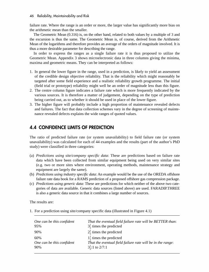
46 Reliability, Maintainability and Risk
failure rate. Where the range is an order or more, the larger value has significantly more bias onthe arithmetic mean than the smaller.
The Geometric Mean (0.316) is, on the other hand, related to both values by a multiple of 3 andthe excursion is thus the same. The Geometric Mean is, of course, derived from the ArithmeticMean of the logarithms and therefore provides an average of the orders of magnitude involved. It isthus a more desirable parameter for describing the range.
In order to express the ranges as a single failure rate it is thus proposed to utilize theGeometric Mean. Appendix 3 shows microelectronic data in three columns giving the minima,maxima and geometric means. They can be interpreted as follows:
1. In general the lower figure in the range, used in a prediction, is likely to yield an assessmentof the credible design objective reliability. That is the reliability which might reasonably betargeted after some field experience and a realistic reliability growth programme. The initial(field trial or prototype) reliability might well be an order of magnitude less than this figure.
2. The centre column figure indicates a failure rate which is more frequently indicated by thevarious sources. It is therefore a matter of judgement, depending on the type of predictionbeing carried out, as to whether it should be used in place of the lower figure.
3. The higher figure will probably include a high proportion of maintenance revealed defectsand failures. The fact that data collection schemes vary in the degree of screening of mainte-nance revealed defects explains the wide ranges of quoted values.
4.4 CONFIDENCE LIMITS OF PREDICTION
The ratio of predicted failure rate (or system unavailability) to field failure rate (or systemunavailability) was calculated for each of 44 examples and the results (part of the author’s PhDstudy) were classified in three categories:
(a) Predictions using site/company specific data: These are predictions based on failure ratedata which have been collected from similar equipment being used on very similar sites(e.g. two or more sites where environment, operating methods, maintenance strategy andequipment are largely the same).
(b) Predictions using industry specific data: An example would be the use of the OREDA offshorefailure rate data book for a RAMS prediction of a proposed offshore gas compression package.
(c) Predictions using generic data: These are predictions for which neither of the above two cate-gories of data are available. Generic data sources (listed above) are used. FARADIP.THREEis also a generic data source in that it combines a large number of sources.
The results are:
1. For a prediction using site/company specific data (illustrated in Figure 4.1)
One can be this confident That the eventual field failure rate will be BETTER than:95% 3 times the predicted
90% 2 times the predicted
60% 1 times the predictedOne can be this confident That the eventual field failure rate will be in the range:90% 3 :1 to 2/7:11
2
12
12
12
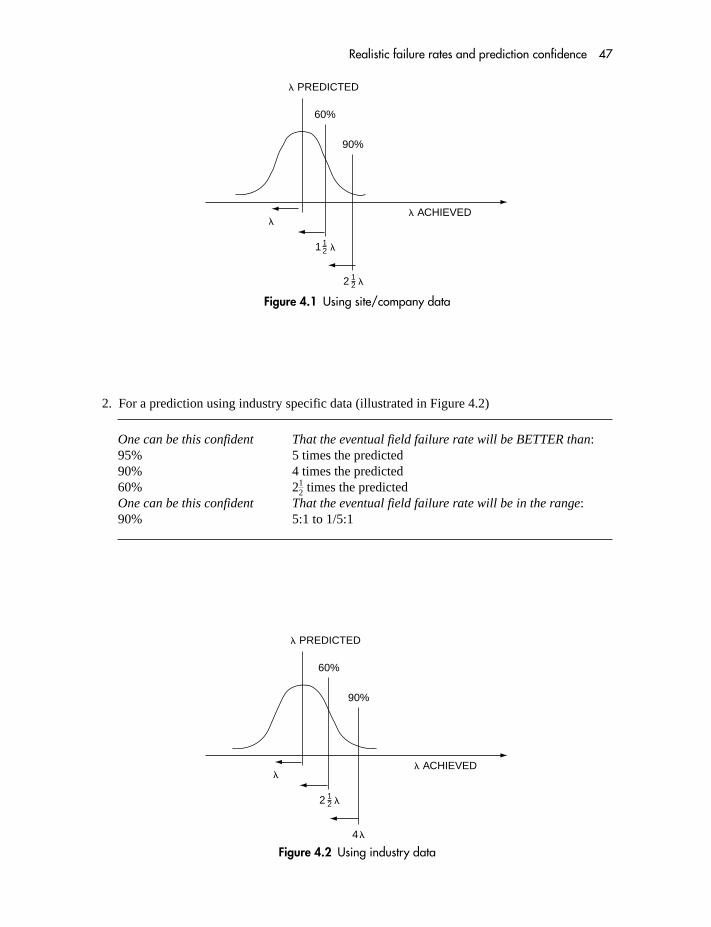
Realistic failure rates and prediction confidence 47
Figure 4.1 Using site/company data
Figure 4.2 Using industry data
� PREDICTED
� ACHIEVED
60%
90%
�
1 �
2 �
12
12
� PREDICTED
� ACHIEVED
60%
90%
4 �
�
2 �12
2. For a prediction using industry specific data (illustrated in Figure 4.2)
One can be this confident That the eventual field failure rate will be BETTER than:95% 5 times the predicted90% 4 times the predicted60% 2 times the predictedOne can be this confident That the eventual field failure rate will be in the range:90% 5:1 to 1/5:1
12

48 Reliability, Maintainability and Risk
Figure 4.3 Using generic data
3. For a prediction using generic data (illustrated in Figure 4.3)
One can be this confident That the eventual field failure rate will be BETTER than:95% 8 times the predicted90% 6 times the predicted60% 3 times the predictedOne can be this confident That the eventual field failure rate will be in the range:90% 8:1 to 1/8:1
Additional evidence in support of the 8:1 range is provided from the FARADIP data bankwhich suggests 7:1.
It often occurs that mixed data sources are used for a RAMS prediction such that, for exam-ple, site/company specific data are available for a few component parts but generic data areused for the other parts. The confidence range would then be assessed as follows:
If Ranges and Rangeg are the confidence ranges for the site/company specific and genericdata expressed as a multiplier then the range for a given prediction becomes
where and are the total failure rates of the site/company specific and generic itemsrespectively.
For example, using the 3 :1 and 8:1 ranges (90% confidence) given above, if permillion hrs (pmh) and pmh, the range for the prediction (at 90% confidence)would be:
At the end of Chapter 9 these ranges are used to compare predictions with targets.
(20 � 3.5) � (100 � 8)
120� 7.25:1
�g � 100�s � 201
2
�g�s
(�s � Ranges) � (�g � Rangeg)
�s � �g
� PREDICTED
� ACHIEVED
60%
90%
3 �
6 �
�

Realistic failure rates and prediction confidence 49
4.5 OVERALL CONCLUSIONS
The use of stress-related regression models, implies an unjustified precision in estimating thefailure rate parameter.
Site/company specific data should be used in preference to industry specific data which, inturn, should be used in preference to generic data.
Predictions should be expressed in confidence limit terms (Section 9.6) using the aboveinformation.
The FARADIP.THREE software package provides maximum and minimum rates togetherwith failure modes.
In practice, failure rate is a system level effect. It is closely related to but not entirelyexplained by component failure. A significant proportion of failures encountered with modernelectronic systems are not the direct result of parts failures but of more complex interactionswithin the system. The reason for this lack of precise mapping arises from such effects ashuman factors, software, environmental interference, interrelated component drift and circuitdesign tolerance.
The primary benefit to be derived from reliability engineering is the reliability growth whicharises from continuing analysis and follow-up as well as corrective actions following failureanalysis. Reliability prediction, based on the manipulation of failure rate data, involves so manypotential parameters that a valid repeatable model for failure rate estimation is not possible.Thus, failure rate is the least accurate of engineering parameters and prediction from past datashould be carried out either:
� As an indicator of the approximate level of reliability of which the design is capable, givenreliability growth in the field.
� To provide relative comparisons in order to make engineering decisions concerning optimumredundancy.
� As a contractual requirement.� In response to safety-integrity requirements.
It should not be regarded as an accurate indicator of future field reliability.
5 Interpreting dataand demonstrating reliability
5.1 THE FOUR CASES
In the following table it can be seen that there are four cases to be considered when interpretingthe k failures and T hours. First, there may be reason to assume constant failure rate whichincludes two cases. If k is large (say, more than 10) then the sampling inaccuracy in such awide-tolerance parameter may be ignored. Chapter 4 has emphasized the wide ranges whichapply and thus, for large values of k the formulae:
� � k/T and � � T/k
can be used. When k is small (even 0), the need arises to make some statistical interpretation ofthe data and that is the purpose of this chapter. The table also shows the second case where con-stant failure rate cannot be assumed. Again there may be few or many failures to interpret.Chapter 6 deals with this problem where the concept of a failure rate is not suitable to describethe failure distribution.
Constant Failure Rate Variable Failure Rate
Few Failures Chapter 5 (Statistical interpretation) Chapter 6 (Inadequate data)Many Failures Chapter 4 (Use � � k/T) Chapter 6 (Use probability plotting)
5.2 INFERENCE AND CONFIDENCE LEVELS
In Section 2.2 the concept of a point estimate of failure rate or MTBF was introduced. Inthe Figure 2.2 N items showed k failures in T cumulative hours and the observed MTBF of thatsample measurement was T/k. If the test were repeated, and another value of T/k obtained, it wouldnot be exactly the same as the first and, indeed, a number of tests would yield a number of valuesof MTBF. Since these estimates are the result of sampling they are called point estimates and havethe symbol . It is the true MTBF of the batch which is of interest and the only way to obtain it isto allow the entire batch to fail and then to evaluate T/k. This is why, the theoretical expression forMTBF in equation (2.5) of Section 2.3 involves the integration limits 0 and infinity:
MTBF � ��
0
Ns(t)
N dt
�
(�)(�)( �)

Interpreting data and demonstrating reliability 51
Thus, all devices must fail if the true MTBF is to be determined. Such a test will, of course, yieldaccurate data but, alas, no products at the end. In practice, we are forced to truncate tests after agiven number of hours or failures. One is called a time-truncated test and the other a failure-truncated test. The problem is that a statement about MTBF, or failure rate, is required when onlysample data are available. In many cases of high reliability, the time required would be unrealistic.
The process of making a statement about a population of items based on the evidence of a sam-ple is known as statistical inference. It involves, however, the additional concept of confidencelevel. This is best illustrated by means of an example. Figure 5.1 shows a distribution of heights ofa group of people in histogram form. Superimposed onto the histogram is a curve of the normaldistribution. The practice in statistical inference is to select a mathematical distribution whichclosely fits the data. Statements based on the distribution are then assumed to apply to the data.
In the figure there is a good fit between the normal curve, having a mean of 5�10� and a standarddeviation (measure of spread) of 1�, and the heights of the group in question. Consider now, a per-son drawn, at random, from the group. It is permissible to state, from a knowledge of the normaldistribution, that the person will be 5�10� tall or more providing that it is stated that the prediction ismade with 50% confidence. This really means that we anticipate being correct 50% of the time ifwe continue to repeat the experiment. On this basis, an indefinite number of statements can bemade, providing that an appropriate confidence level accompanies each value. For example:
5�11� or more at 15.9% confidence6�0� or more at 2.3% confidence6�1� or more at 0.1% confidence
OR between 5�9� and 5�11� at 68.2% confidence
The inferred range of measurement and the confidence level can, hence, be traded off againsteach other.
5.3 THE CHI-SQUARE TEST
Returning to the estimates of MTBF, it is possible to employ the same technique of stating anMTBF together with a confidence level if the way in which the values are distributed is known.It has been shown that the expression
2k�
� (random failures assumed)
Histogram
Closelyfittingnormalcurve
Height
Num
ber
of p
erso
ns o
fth
e st
ated
hei
ght
5′7″ 5′10″ 6′1″
Figure 5.1 Distribution of heights

52 Reliability, Maintainability and Risk
follows a �2 distribution with 2k degrees of freedom, where the test is truncated at the kthfailure. We know already that
Therefore
so that 2T/� is �2 distributed.If a value of �2 can be fixed for a particular test then 2T/�, and hence � can be stated to lie
between specified confidence limits. In practice, the upper limit is usually set at infinity and onespeaks of an MTBF of some value or greater. This is known as the single-sided lower confi-dence limit of MTBF. Sometimes the double-sided limit method is used, although it is moreusual to speak of the lower limit of MTBF.
It is not necessary to understand the following explanation of the �2 distribution. Readerswho wish to apply the technique quickly and simply to the interpretation of data can move
DIRECTLY TO SECTION 5.5
For those who wish to understand the method in a little more detail then Figure 5.2 shows a dis-tribution of �2. The area of the shaded portion is the probability of �2 exceeding that particularvalue at random.
In order to determine a value of �2 it is necessary to specify two parameters. The first is thenumber of degrees of freedom (twice the number of failures) and the second is the confidence level.The tables of �2 at the end of this book (Appendix 2) have columns and rows labelled and n.The confidence level of the �2 distribution is and n is the number of degrees of freedom. Thelimits of MTBF, however, are required between some value, A, and infinity. Since � � 2T/�2 thevalue of �2 corresponding to infinite � is zero. The limits are therefore zero and A. In Figure 5.2,if is the area to the right of A then 1 must be the confidence level of �.
If the confidence limit is to be at 60%, the lower single-sided limit would be that value whichthe MTBF exceeds, by chance, six times out of 10. Since the degrees of freedom can beobtained from 2k and � (1 0.6) � 0.4, then a value of �2 can be obtained from the tables.
From 2T/�2 it is now possible to state a value of MTBF at 60% confidence. In other words,such a value of MTBF or better would be observed 60% of the time. It is written �60%.Alternatively �60% � �2/2T.
2k�
� �
2kT
k��
2T
�
� �T
k�
Accumulated test hours
Number of failures
Figure 5.2 Single-sided confidence limits

Interpreting data and demonstrating reliability 53
In a replacement test (each failed device is replaced immediately) 100 devices are tested for1000 h during which three failures occur. The third failure happens at 1000 h at which point thetest is truncated. We shall now calculate the MTBF of the batch at 90% and 60% confidencelevels.
1. Since this is a replacement test T is obtained from the number under test multiplied by thelinear test time. Therefore T � 100 000 h and k � 3.
2. Let n � 2k � 6 degrees of freedom. For 90% confidence � (1 0.9) � 0.1 and for 60%confidence � 1 0.6 � 0.4.
3. Read off �2 values of 10.6 and 6.21 (see Appendix 2).4. �90% � 2 � 100 000/10.6 � 18 900 h.
�60% � 2 � 100 000/6.21 � 32 200 h.
Compare these results with the original point estimate of T/k � 100 000/3 � 33 333 h. It ispossible to work backwards and discover what confidence level is actually applicable to thisestimate. �2 � 2T/� � 200 000/33 333 � 6. Since n is also equal to 6 it is possible to consultthe tables and see that this occurs for a value of slightly greater than 0.4. The confidence withwhich the MTBF may be quoted as 33 333 h is therefore less than 60%. It cannot be assumedthat all point estimates will yield this value and, in any case, a proper calculation, as outlined,should be made.
In the above example the test was failure truncated. For a time-truncated test, one must beadded to the number of failures (two to the degrees of freedom) for the lower limit of MTBF.This takes account of the possibility that, had the test continued for a few more seconds, a fail-ure might have occurred. In the above single-sided test, the upper limit is infinity and the valueof MTBF is, hence, the lower limit. A test with zero failures can now be interpreted.
Consider 100 components for 50 h with no failures. At a 60% confidence we have�60% � 2T/�2 � 2 � 50 � 100/�2. Since we now have � 0.4 and n � 2(k � 1) � 2,�2 � 1.83 and � � 10 000/1.83 � 5 464 h. Suppose that an MTBF of 20 000 h wasrequired. The confidence with which it has been proved at this point is calculated as before.�2 � 2T/� � 20 000/20 000 � 1. This occurs at � 0.6, therefore the confidence stands at40%. If no failures occur then, as the test continues, the rise in confidence can be computedand observed. Furthermore, the length of the test (for zero failures) can be calculated inadvance for a given MTBF and confidence level.
5.4 DOUBLE-SIDED CONFIDENCE LIMITS
So far, lower single-sided statements of MTBF have been made. Sometimes it is required tostate that the MTBF lies between two confidence limits. Once again � (1 – confidence level)and is split equally on either side of the limits as shown in Figure 5.3.
The two values of �2 are found by using the tables twice, first at n � 2k and at 1 /2(this gives the lower limit of �2) and second at n � 2k (2k � 2 for time truncated) and at /2(this gives the upper limit of �2). Once again, the upper limit of �2 corresponds with thelower limit of MTBF and vice versa. Figure 5.3 shows how /2 and 1 /2 are used. Theprobabilities of �2 exceeding the limits are the areas to the right of each limit and the tablesare given accordingly.
Each of the two values of �2 can be used to obtain the limits of MTBF from the expression� � 2T/�2. Assume that the upper and lower limits of MTBF for an 80% confidence band are

54 Reliability, Maintainability and Risk
required. In other words, limits of MTBF are required such that 80% of the time it will fallwithin them. T � 100 000 h and k � 3. The two values of �2 are obtained:
n � 6, � 0.9, �2 � 2.2n � 8, � 0.1, �2 � 13.4
This yields the two values of MTBF – 14 925 h and 90 909 h, in the usual manner, from theexpression � � 2T/�2.
Hence the MTBF lies between 14 925 and 90 909 h with a confidence of 80%.
5.5 SUMMARIZING THE CHI-SQUARE TEST
The following list of steps summarizes the use of the �2 tables for interpreting the results ofreliability tests:
Figure 5.3 Double-sided confidence limits
1. Measure T (accumulated test hours) and k (number of failures).2. Select a confidence level and let � � (1 � confidence level).3. Let n � 2k (2k � 2) for lower limit MTBF in time-truncated test.4. Note the value of �2 from the tables at the end of this book (Appendix 2).5. Let MTBF at the given confidence level be 2T/�2 or �60% � �2/2T.6. For double-sided limits use the above procedure twice at
n � 2k:1 � � /2 (upper limit of MTBF)n � 2k(2k � 2):� /2 (lower limit of MTBF)
It should be noted that, for constant failure rate conditions, 100 components under test for20 h yield the same number of accumulated test hours as 10 components for 200 h. Othermethods of converting test data into statements of MTBF are available but the �2 distributionmethod is the most flexible and easy to apply. MTBFs are usually computed at the 60% and90% confidence levels.
5.6 RELIABILITY DEMONSTRATION
Imagine that, as a manufacturer, you have evaluated the MTBF of your components at someconfidence level using the techniques outlined, and that you have sold them to me on the basis ofsuch a test. I may well return, after some time, and say that the number of failures experienced in

Interpreting data and demonstrating reliability 55
a given number of hours yields a lower MTBF, at the same confidence, than did your earlier test.You could then suggest that I wait for another month, by which time there is a chance that thenumber of failures and the number of test hours will have swung the calculation in your favour.Since this is hardly a suitable way of doing business, it is necessary for consumer and producerto agree on a mutually acceptable test for accepting or rejecting batches of items. Once the testhas been passed there is to be no question of later rejection on discovering that the batch passedon the strength of an optimistic sample. On the other hand, there is no redress if the batch isrejected, although otherwise acceptable, on the basis of a pessimistic sample. The risk that thebatch, although within specification, will fail owing to a pessimistic sample being drawn isknown as the producer’s risk and has the symbol (not to be confused with the in the previoussection). The risk that a ‘bad’ batch will be accepted owing to an optimistic sample is known asthe consumer’s risk, . The test consists of accumulating a given number of test hours and thenaccepting or rejecting the batch on the basis of whether or not a certain number of failures havebeen observed.
Imagine such a test where the sample has to accumulate T test hours with no failures inorder to pass. If the failure rate, �, is assumed to be constant then the probability of observingno failures in T test hours is e�T (from the Poisson distribution). Such a zero failures test isrepresented in Figure 5.4, which is a graph of the probability of observing no failures (in otherwords, of passing the test) against the anticipated number of failures given by �T. This type oftest is known as a Fixed-Time Demonstration Test. It can be seen from the graph that, as thefailure rate increases, the probability of passing the test falls.
The problem with this type of testing is the degree of discrimination. This depends on thestatistical risks involved which are highlighted by the following example.
Assume, for the sake of argument, that the acceptable proportion of bad eggs (analogous tofailure rate) is 104 (one in 10 000). If the reader were to purchase 6 eggs each week then he orshe would be carrying out a demonstration test with a zero failures criterion. That is, with nobad eggs all is well, but if there is but one defective then a complaint will ensue. On the surface,this appears to be a valid test which carries a very high probability of being passed if the pro-portion of bad eggs is as stated.
Consider, however, the situation where the proportion increases to 103, in other words byten times. What of the test? The next purchase of 6 eggs is very unlikely to reveal a defect. Thistest is therefore a poor discriminator and the example displays, albeit lightheartedly, the prob-lem of demonstrating a very high reliability (low failure rate). In many cases a statisticaldemonstration can be totally unrealistic for the reasons described above.
A component has an acceptable failure rate of 300 � 109/h (approx. 1 in 380 yr). Fifty aretested for 1000 h (approx. 5 years of test). �T is therefore
5.5
380� 0.014 and the probability of passing the test is e0.014 � 98.6%.
12
Probability ofpassing thetest
1
00 �T
Figure 5.4 Zero failures test

56 Reliability, Maintainability and Risk
Suppose that a second test is made from a batch whose failure rate is three times that of the firstbatch (i.e. 900 � 109/h). Now the probability of passing the test is e�T � e0.043 � 95.8%.Whereas the acceptable batch is 98.6% sure of acceptance ( � 1.4%) the ‘bad’ batch is only4.2% sure of rejection ( � 95.8%). In other words, although the test is satisfactory for passingbatches of the required failure rate, it is a poor discriminator whose acceptance probability doesnot fall sufficiently quickly as the failure rate increases.
A test is required which not only passes acceptable batches (a sensible producer’s risk wouldbe between 5% and 15%) but rejects batches with a significantly higher failure rate. Threetimes the failure rate should reduce the acceptance probability to 15% or less. The only waythat this can be achieved is to increase the test time so that the acceptance criterion is muchhigher than zero failures (in other words, buy many more eggs!).
In general, the criterion for passing the test is n or fewer failures and the probability of passingthe test is:
This expression yields the family of curves shown in Figure 5.5, which includes the specialcase (n � 0) of Figure 5.4. These curves are known as Operating Characteristics (OC Curves),each one representing a test plan.
Each of these curves represents a valid test plan, and to demonstrate a given failure rate thereis a choice of 0, 1, 2, 3, . . . , n failure criterion tests with corresponding values of T. The higherthe number of failures, the greater the number of test hours are required. Figure 5.6 shows theimprovement in discrimination as n increases. Note that n is replaced by c, which is the usualconvention. The extreme case where everything is allowed to fail and c equals the population isshown. Since there is no question of uncertainty under these circumstances, the probability ofpassing the test is either one or zero, depending upon the batch failure rate. The question ofsampling risks does not arise.
Consider the c � 0 plan and note that a change from �0 to 3�0 produces little decrease inthe acceptance probability and hence a poor consumer’s risk. If the consumer’s risk wereto be 10% the actual failure rate would be a long way to the right on the horizontal axisand would be many times �0. This ratio is known as the Reliability Design Index orDiscrimination Ratio. Looking, now, at the c � 5 curve, both producer and consumer risksare reasonable for a 3:1 change in failure rate. In the extreme case of 100% failures both risksreduce to zero.
P0n � �n
i � 0 �iT ie�T
i!
Pro
babi
lity
of p
assi
ng th
e te
st 1
0
n = 0 n = 1 n = 2 n = 3
0�T
Figure 5.5 Family of OC curves

Interpreting data and demonstrating reliability 57
Figure 5.7 is a set of Cumulative Poisson Curves which enable the test plans and risks to beevaluated as in the following example.
A failure rate of 3 � 104/h is to be demonstrated using 10 items. Calculate the number oftest hours required if the test is to be passed with 4 or fewer failures and the probability ofrejecting acceptable items () is to be 10%:
1. Probability of passing test � 1 0.1 � 0.9.2. Using Figure 5.7 the corresponding value for c � 4 at 0.9 is 2.45.3. �T � 3 � 104 � T � 2.45. Therefore T � 8170 h.4. Since there are 10 items the test must last 817 h with no more than four failures.
If the failure rate is three times the acceptable value, calculate the consumer’s risk, :
1. 3�T � 3 � 3 � 104 � 8170 � 7.35.2. Using Figure 5.7 for m � 7.35 and c � 4:P04 � 0.15.3. The consumer’s risk is therefore 15%.
Readers might care to repeat this example for a zero failures test and verify for themselvesthat, although T is as little as 333 h, rises quickly to 74%. The difficulty of high-reliabilitytesting can now be appreciated. For example, equipment which should have a one-year MTBFrequires at least 3 years of testing to demonstrate its MTBF with acceptable risks. If only oneitem is available for test then the duration of the demonstration would be 3 years. In practice,far larger MTBFs are aimed for, particularly with submarine and satellite systems, and demon-stration testing as described in this chapter is not applicable.
5.7 SEQUENTIAL TESTING
The above type of test is known as a Fixed-Time Demonstration. Owing to the difficulties ofdiscrimination, any method that results in a saving of accumulated test hours without changingany of the other parameters is to be welcomed.
Experience shows that the Sequential Demonstration Test tends to achieve results slightlyfaster than the equivalent fixed-time test. Figure 5.8 shows how a sequential reliability test is
Figure 5.6 OC curves showing discrimination

58 Reliability, Maintainability and Risk
operated. Two parallel lines are constructed so as to mark the boundaries of the three areas –Accept, Reject and Continue Testing. As test hours are accumulated the test proceeds along thex-axis and as failures occur the line is moved vertically one unit per failure. Should the test linecross the upper boundary, too many failures have been accrued for the hours accumulated andthe test has been failed. If, on the other hand, the test crosses the lower boundary, sufficient test
Figure 5.7 Cumulative Poisson curves

Interpreting data and demonstrating reliability 59
hours have been accumulated for the number of failures and the test has been passed. As long asthe test line remains between the boundaries the test must continue.
Should a time limit be set to the testing then a truncating line is drawn as shown to the rightof the diagram so that, if the line crosses above the mid-point, the test has been failed. If, asshown, it crosses below the mid-point, the test has been passed. If a decision is made by cross-ing the truncating line rather than one of the boundary lines, then the consumer and producerrisks calculated for the test no longer apply and must be recalculated.
As in the fixed-time test, the consumer’s risk, producer’s risk and the MTBF associated witheach are fixed. The ratio of the two MTBFs (or failure rates) is the reliability design index. Thelines are constructed from the following equations:
provided and are small (less than 25%).The equation for ylower is the same with loge B substituted for loge A. If the risks are reduced
then the lines move further apart and the test will take longer. If the design index is reduced,bringing the two MTBFs closer together, then the lines will be less steep, making it harder topass the test.
5.8 SETTING UP DEMONSTRATION TESTS
In order to conduct a demonstration test (sometimes called a verification test) the followingconditions, in addition to the statistical plans already discussed, must be specified:
1. Values of consumer’s risk and acceptable MTBF. The manufacturer will then decide on therisk and upon a reliability design index. This has already been examined in this chapter. Afailure distribution must be agreed (this chapter has dealt only with random failures). A testplan can then be specified.
2. The sampling procedure must be defined in terms of sample size and from where and howthe samples should be drawn.
3. Both environmental and operational test conditions must be fixed. This includes specifyingthe location of the test and the test personnel.
yupper �(1/�1) (1/�0)
loge (�0/�1) T �
loge A
loge (�0/�1) : A ≈
1
and B ≈
1
Figure 5.8 Truncated sequential demonstration test

60 Reliability, Maintainability and Risk
4. Failure must be defined so that there will be no argument over what constitutes a failureonce the test has commenced. Exceptions should also be defined, i.e. failures which are to bedisregarded (failures due to faulty test equipment, wrong test procedures, etc.).
5. If a ‘burn-in’ period is to be allowed, in order that early failures may be disregarded, this toomust be specified.
The emphasis in this chapter has been on component testing and demonstration, but if equip-ment or systems are to be demonstrated, the following conditions must also be specified:
1. Permissible corrective or preventive maintenance during the test (e.g. replacement of partsbefore wearout, routine care).
2. Relevance of secondary failures (failures due to fluctuations in stress caused by other failures).3. How test time relates to real time (24 h operation of a system may only involve 3 h of operation
of a particular unit).4. Maximum setting-up and adjustment time permitted before the test commences.
US Military Standard 781C – Reliability Design Qualification and Production AcceptanceTests – contains both fixed time and sequential test plans. Alternatively, plans can be easilyconstructed from the equations and curves given in this chapter.
EXERCISES
1. A replacement test involving 50 devices is run for 100 h and then truncated. Calculate theMTBF (single-sided lower limit) at 60% confidence:(a) If there are two failures;(b) If there are zero failures.
2. The items in Exercise 1 are required to show an MTBF of 5000 h at 90% confidence. Whatwould be the duration of the test, with no failures, to demonstrate this?
3. The producer’s risk in a particular demonstration test is set at 15%. How many hours mustbe accumulated, with no failures, to demonstrate an MTBF of 1000 h? What is the result if abatch is submitted to the test with an MTBF of 500 h? If the test were increased to five fail-ures what would be the effect on T and ?

6 Variable failure ratesand probability plotting
6.1 THE WEIBULL DISTRIBUTION
The Bathtub Curve in Figure 2.5 showed that, as well as random failures, there are distributionsof increasing and decreasing failure rate. In these variable failure rate cases it is of little value toconsider the actual failure rate since only Reliability and MTBF are meaningful. In Chapter 2we saw that:
Since the relationship between failure rate and time takes many forms, and depends on thedevice in question, the integral cannot be evaluated for the general case. Even if the variation offailure rate with time were known, it might well be of such a complicated nature that the inte-gration would prove far from simple.
In practice it is found that the relationship can usually be described by the following three-parameter distribution known as the Weibull distribution named after Professor WaloddiWeibull:
In many cases a 2 parameter model proves sufficiently complex to describe the data.Hence:
The constant failure rate case is the special one-parameter case of the Weibull distribution.Only randomness can be described by a single parameter.
In the general Weibull case, the reliability function requires three parameters (�, �, �). Theydo not have physical meanings in the same way as does failure rate. They are parameters whichallow us to compute Reliability and MTBF. In the special case of � � 0 and � � 1 the expres-sion reduces to the exponential case with � giving the MTBF. In the general case, however, � isnot the MTBF and is known as the scale parameter. � is known as the shape parameter anddescribes the rate of change of failure rate, increasing or decreasing. � is known as the locationparameter, in other words a displacement of the time origin. � � 0 means that the time originis, in fact, at t � 0.
R(t) � exp [�(t/�)�]
R(t) � exp ���t � �
� ��
�
R(t) � exp ���t
0
�(t) dt�

62 Reliability, Maintainability and Risk
The following equations show how data which can be described by a Weibull function can bemade to fit a straight line. It is not essential to follow the explanation and the reader may, ifdesired, move to the next block of text.
The Weibull expression can be reduced to a straight-line equation by taking logarithms twice:
If 1 � R(t) � Q(t) . . . the unreliability (probability of failure in t)
then
so that
Therefore
and
which is Y � mX � C, the equation of a straight line.If (t � �) is replaced by t then:
.
If Y � 0
then
so that
This occurs if
loglog 1
1 � Q(t)� 0 so that log
1
1 � Q(t)� 1
t � �
� log t � � log �
loglog 1
1 � Q(t) � 0
Y � loglog 1
1 � Q(t) and X � log t and the slope m � �
loglog 1
1 � Q(t) � � log (t � �) � � log �
log 1
1 � Q(t)� �t � �
� ��
1
1 � Q(t)� exp �t � �
� ��
1 � Q(t) � exp ���t � �
� ��
�

Variable failure rates and probability plotting 63
i.e.
If a group of failures is distributed according to the Weibull function and it is initiallyassumed that � � 0, then by plotting these failures against time on double logarithmic paper(failure percentage on loglog scale and time on log scale), a straight line should be obtained.The three Weibull parameters and hence the expression for Reliability may then be obtainedfrom measurements of the slope and intercept.
Figure 6.1 is loglog by log graph paper with suitable scales for cumulative percentage failure andtime. Cumulative percentage failure is effectively the unreliability and is estimated by taking eachfailure in turn from median ranking tables of the appropriate sample size. It should be noted thatthe sample size, in this case, is the number of failures observed. However, a test yielding 10 failuresfrom 25 items would require the first 10 terms of the median ranking table for sample size 25.
6.2 USING THE WEIBULL METHOD
6.2.1 Curve fitting to interpret failure data
Assume that the failure rate is not constant OR, alternatively, that we want to determinewhether it is or not.
Whereas, in the case of random failures (dealt with in Chapter 5) it was only necessary toknow the total time T applying to the k failures, it is now necessary to know the individualtimes to failure of the items. Without this information it would not be possible to fit the data toa distribution.
The Weibull technique assumes, initially, that the distribution of failures, whilst not random,is at least able to be modelled by a simple 2 parameter distribution. It assumes that:
The technique is to carry out a curve fitting (probability modelling) exercise to establish firstthat the data will fit this assumption and second to estimate the values of the 2 parameters.
Traditionally this has been done by ‘pencil and paper’ curve fitting methods which aredescribed here. In a later section a software tool, for performing this task, is described.
If � � 1 then the failures are random and a constant failure rate can be assumed wherefailure rate � 1/�.
If � 1 then the failure rate is increasing.
If � � 1 then the failure rate is decreasing.
In some cases, where the 2 parameter distribution is inadequate to model the data, the3 parameter version can be used. In that case:
� can be estimated by successive iteration until a fit to the 2 parameter distribution is obtained.This will be described in Section 6.3.
R(t) � exp � [(t � �)/�]�
R(t) � exp � (t/�)�
1
1 � Q(t)� e and Q(t) � 0.63

64 Reliability, Maintainability and Risk
Figu
re 6
.1G
raph
pap
er fo
r W
eibu
ll pl
ot

Variable failure rates and probability plotting 65
6.2.2 Manual plotting
Ten devices were put on test and permitted to fail without replacement. The time at which eachdevice failed was noted and from the test information we require to determine:
1. If there is a Weibull distribution which fits these data;2. If so, the values of �, � and �;3. The probability of items surviving for specified lengths of time;4. If the failure rate is increasing, decreasing or constant;5. The MTBF.
The results are shown in Table 6.1 against the median ranks for sample size 10. The ten pointsare plotted on Weibull paper as in Figure 6.2 and a straight line is obtained.
The straight line tells us that the Weibull distribution is applicable and the parameters aredetermined as follows:
�: It was shown in Section 6.1 that if the data yield a straight line then � � 0.�: The slope yields the value of � which is obtained by taking a line parallel to the data line but
through the origin of the construction in Figure 6.2. The value of � is shown by the intersec-tion with the arc. Here � � 1.5.
�: We have already shown that � � t for Q(t) � 0.63, hence � is obtained by taking a hori-zontal line from the origin of the construction across to the data line and then reading thecorresponding value of t.
Table 6.1
Cumulative failures, 6.7 16.2 25.9 35.6 45.2 54.8 64.5 74.1 83.8 93.3Qt (%) median rank
Time, t (hours � 100) 1.7 3.5 5.0 6.4 8.0 9.6 11 13 18 22
Figure 6.2 Results plotted on Weibull paper

66 Reliability, Maintainability and Risk
The reliability expression is therefore:
The probability of survival to t � 1000 h is therefore:
R(1000) � e�0.855 � 42.5%
The test shows a wearout situation since �, which is known as the shape parameter, 1.
For increasing failure rate � 1For decreasing failure rate � � 1For constant failure rate � � 1
It now remains to evaluate the MTBF. This is, of course, the integral from zero to infinity ofR(t). Table 6.2 enables us to short cut this step.
Since � � 1.5 then MTBF/� � 0.903 and MTBF � 0.903 � 1110 � 1002 h. Since medianrank tables have been used, the MTBF and reliability values calculated are at the 50% confi-dence level. In the example, time was recorded in hours but there is no reason why a moreappropriate scale should not be used such as number of operations or cycles. The MTBF wouldthen be quoted as Mean Number of Cycles between Failures.
For samples of other than 10 items, a set of median ranking tables is required. Since spacedoes not permit a full set to be included the following approximation is given. For sample sizeN the r th rank is obtained from Bernard’s approximation:
Care must be taken in the choice of the appropriate ranking table. N is the number of items inthe test and r the number that failed, in other words, the number of data points. In our example
r � 0.3
N � 0.4
R(t) � exp ��� t
1110�1.5�
Table 6.2
� � � �
0.0 1.0 1.000 2.0 0.886 3.0 0.8940.1 10! 1.1 0.965 2.1 0.886 3.1 0.8940.2 5! 1.2 0.941 2.2 0.886 3.2 0.8960.3 9.261 1.3 0.923 2.3 0.886 3.3 0.8970.4 3.323 1.4 0.911 2.4 0.886 3.4 0.8980.5 2.000 1.5 0.903 2.5 0.887 3.5 0.9000.6 1.505 1.6 0.897 2.6 0.888 3.6 0.9010.7 1.266 1.7 0.892 2.7 0.889 3.7 0.9020.8 1.133 1.8 0.889 2.8 0.890 3.8 0.9040.9 1.052 1.9 0.887 2.9 0.892 3.9 0.905
4.0 0.906
MTBF�
MTBF�
MTBF�
MTBF�

Variable failure rates and probability plotting 67
N was 10 not because the number of failures was 10 but because it was the sample size. As it hap-pens, we considered the case where all 10 failed.
Had there been 20 items, of which 10 did not fail, the median ranks from Bernard’s formulawould have been:
%:– 3.4 8.3 13 18 23 28 33 38 43 48
Although this method allows for the ranking of the failures it does not take account of theactual hours contributed by the censored items. In the next section, the Maximum Likelihoodtechnique is introduced partly for this purpose.
6.2.3 Using a computer method
The COMPARE software package provides a method of probability plotting whereby Weibullparameters are found which best fit the data being analysed.
Repair times and censored data are entered and estimates of the Weibull parameters, as wellas a graphical plot, are provided.
There are four types of censoring:
1. Items removed (for some reason other than failure) before the test finishes.2. Items which continue after the last failure.3. Items which are added after the commencement of the test whose operating hours count
from their inclusion.4. Failed items which are restored to ‘as new’ condition and then clock up further operating time.
Strictly speaking this is not an example of censoring since the item has been allowed to fail.
In the latter case it is important to be satisfied that the refurbishment really is ‘as new’. If sothe additional hours count from the refurbishment and are treated as an extra item.
In practice it may happen that there is a time to failure for a particular failure mode. Theitem might be repaired ‘as new’ and continue until it fails again. IMPORTANT – If the secondfailure is the same mode then the time to failure is counted from the refurbishment. If thesecond failure is a different mode then the time to failure is the whole operating time from thecommencement of the test.
It MUST be remembered, however, that any computerized algorithm will allocate parametersto any data for a given distribution. It is, therefore, important to be aware of the limitations ofprobability plotting.
Two methods of estimating the Weibull parameters from a set of times to failure are LEASTSQUARES AND MAXIMUM LIKELIHOOD.
The Least Squares method is used as an initial calculation and involves calculating the hypothet-ical line for which the sum of the squares of the distances of the horizontal distances from the datapoints to the line is a minimum. The Weibull parameters, BETA and ETA, are obtained from theline. For the two-parameter Weibull distribution, the Least Squares estimates are obtained from:
where
t � timeX � loge tY � loge {loge[1/(1 � F(t))]}
ETA � exp (X � Y/Beta)
BETA � (�(Yi)2 � Y �Yi)/(�(XiYi � X �Yi)

68 Reliability, Maintainability and Risk
Because this Least Squares method involves treating each of the squared distances withequal importance, it favours the higher values of time. Nevertheless, the Least Squaresestimates of BETA and ETA may well be adequate if there is very little, or better still, nocensored data. However data sets usually involve some times to failure (the failed items)and some times with no failure (the survivors). In this case the MAXIMUM LIKELIHOODestimate is required.
In COMPARE, the Least Squares estimates of BETA and ETA are used as the most reason-able estimate for commencing the iterative process of determining Maximum Likelihood valueswhich give equal weight to each data point by virtue of calculating its probability of causing theestimated parameter. The algorithm generates the Weibull BETA and ETA parameters fromwhich the data are most likely to have come by setting up a likelihood equation, differentiatingwith respect to BETA and ETA, and setting this equal to zero (in other words the standard cal-culus method of obtaining a minimum). The process is iterated for alternate BETA and ETAestimates until the values do not significantly change.
The Maximum Likelihood values are then taken as the best estimates of the Weibullparameters.
A large number of data collection schemes do not readily provide the times to failure of theitems in question. For example, if an assembly (such as a valve) is replaced from time to timethen its identity and its time to failure and replacement might be obtainable from the data.However, it might well be the diaphragm which is eventually the item of interest. Diaphragmsmay have been replaced during routine maintenance and the identity of each diaphragm notrecorded. Subsequent Weibull analysis of the valve diaphragm would not then be possible.Careful thought has to be given when implementing a data collection scheme as to what subse-quent DATA ANALYSIS will take place.
As in the above example of a valve and its diaphragm each of SEVERAL FAILUREMODES will have its own failure distribution for which Weibull analysis may be appropriate.It is very likely, when attempting this type of modelling, that data not fitting the 2 parameterdistribution actually contains more than one failure mode. Separating out the individual failuremodes may permit successful Weibull modelling.
6.2.4 Significance of the result
The dangers of attempting to construct a Weibull plot with too few points should be noted. Asatisfactory result will not be obtained with less than at least six points. Tests yielding 0, 1, 2and even 3 failures do not allow a variable failure rate to be observed. In these cases constantfailure rate must be assumed and the Chi-square test used which is a valid approach providedthat the information extracted is applied only to the same time range as the test.
The comparison between the results obtained from Least Squares and Maximum Likelihoodestimations (described above) provide an initial feel for how good a fit the data is to the inferredWeibull parameters.
If (in addition to the confidence obtained from the physical plot) the two values of ShapeParameter, obtained from Least Squares and Maximum Likelihood, are in good agreement thenthere is a further test.
This is provided by way of the Gnedenko test which tests for constant failure rate. This is an‘F’ test which tests the hypothesis that the failure times are at random, i.e. � � 1. The screen willstate whether or not it is valid to reject the assumption that � � 1. The lower the value of the signifi-cance per cent then the more likely it is that the failure rate is significantly different from constant.
Essentially the test compares the MTTF of the failure times as grouped either side of themiddle failure time and tests for a significant difference.

Variable failure rates and probability plotting 69
If the total number of failure times is n, and the time of the n/2th failure is T, the two esti-mates are:
That is to say we are comparing the MTTF of the ‘first half’ of the failures and the MTTF ofthe ‘second half’. The ratio should be one if the failure rate is constant. If it is not then the mag-nitude of the ratio gives an indication of significance. The ratio follows an ‘F’ distribution andthe significance level can therefore be calculated. The two values of MTTF are shown on thescreen. If this test were applied to the graphical plot in Section 6.2.2, we would see that, despitea fairly good straight line, the confidence that � is not 1 is only 32%!
It should be remembered that a small number of failure times, despite a high value of �, maynot show a significant departure from the ‘random’ assumption. In practice 10 or more failuretimes is a minimum desirable data set for Weibull analysis. Nevertheless, engineering judge-ment should always be used to temper statistical analysis. The latter looks only at numbers anddoes not take account of known component behaviours.
Note: If a poor fit is obtained from the 2 parameter model, and the plot is a simple curverather than ‘S’ shaped or disjointed, then it is possible to attempt a 3 parameter model byestimating the value of � described in section 6.3. The usual approach is to assume that� takes the value of the first failure time and to proceed, as above, with the 2 parametermodel to find � and �. Successive values of � can be attempted, by iteration, until the2 parameter model provides a better fit. It must be remembered however that if the reasonfor a poor fit with the 2 parameter model is that only a few failure times are available thenthe use of the 3 parameter model is unlikely to improve the situation.
If the plot is ‘S’ shaped, then it is possible that two failure modes are present in the data.In the author’s experience only a limited number of components show a significantly increasing
failure rate. This is often due to the phenomenon (known as Drenick’s law) whereby a mixture ofthree or more failure modes will show a random failure distribution irrespective of the BETAs ofthe individual modes.
6.3 MORE COMPLEX CASES OF THE WEIBULL DISTRIBUTION
Suppose that the data in our example had yielded a curve rather than a straight line. It is still pos-sible that the Weibull distribution applies but with � greater than zero. The approach is to selectan assumed value for �, usually the first value of t in the data, and replot the line against t,where t � t � �. The first point is now not available and the line will be constructed from onepoint fewer. Should the result be a straight line then the value of � is as estimated and one pro-ceeds as before to evaluate the other two parameters. Mean Time Between Failure is calculatedas before plus the value of �. If, on the other hand, another curve is generated then a furthervalue of � is tried until, by successive approximations, the correct value is found. This trial anderror method of finding � is not as time consuming as it might seem. It is seldom necessary toattempt more than four approximations of � before either generating a straight line or confirmingthat the Weibull distribution will not fit the data. One possible reason for the Weibull distribution
�n/2
i�1ti � (n/2 � T )
n/2 and �
n
i�n/2�1(ti � T )
n/2

70 Reliability, Maintainability and Risk
not applying could be the presence of more than one failure mechanism in the data. Two mecha-nisms are unlikely to follow the same distribution and it is important to confine the analysis toone mechanism at a time.
So far, a single-sided analysis at 50% confidence has been described. It is possible to plot the90% confidence bands by use of the 5% and 95% rank tables. First, Table 6.3 is constructed andthe confidence bands plotted as follows.
Time or number of operations × 100
Cum
ulat
ive
dist
ribut
ion
func
tion,
Q (t
), p
er c
ent
0.10.1
0.2 0.5 1 2 5 10 20 50 100
99.999
90
0.0
0.5
1.0
2.03.0
4.0
A
A´
B
B´
7050
20
10
5
2
1
0.5
0.2
Table 6.3
Time, t (hours � 100) 1.7 3.5 5.0 6.4 8.0 9.6 11 13 18 22Median rank 6.7 16.2 25.9 35.6 45.2 54.8 64.5 74.1 83.8 93.35% rank 0.5 3.7 8.7 15 22 30 39 49 61 7495% rank 26 39 51 61 70 78 85 91 96 99
Figure 6.3 Ninety per cent confidence bands
Consider the point corresponding to the failure at 500 h. The two points A and B are marked onthe straight line corresponding to 8.7% and 51% respectively. The median rank for this point was25.9% and vertical lines are drawn from A and B to intersect the horizontal. These two points lieon the confidence bands. The other points are plotted in the same way and confidence bands areproduced as shown in Figure 6.3. Looking at the curves, the limits of Q(t) at 1000 h are 30% and85%. At 90% confidence the Reliability for 1000 h is therefore between 15% and 70%.
6.4 CONTINUOUS PROCESSES
There is a very strict limitation to the use of this Weibull method, which is illustrated by the case offilament lamps. It is well known that these do not fail at random. Indeed, they have a pronouncedwearout characteristic with a � in excess of two. However, imagine a brand new building with brand
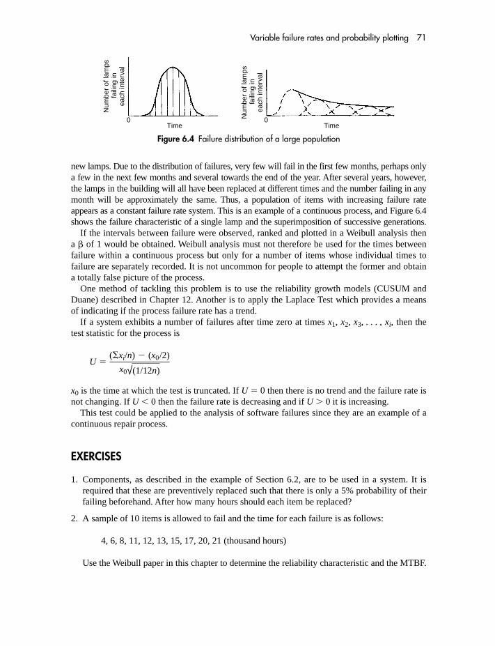
Variable failure rates and probability plotting 71
new lamps. Due to the distribution of failures, very few will fail in the first few months, perhaps onlya few in the next few months and several towards the end of the year. After several years, however,the lamps in the building will all have been replaced at different times and the number failing in anymonth will be approximately the same. Thus, a population of items with increasing failure rateappears as a constant failure rate system. This is an example of a continuous process, and Figure 6.4shows the failure characteristic of a single lamp and the superimposition of successive generations.
If the intervals between failure were observed, ranked and plotted in a Weibull analysis thena � of 1 would be obtained. Weibull analysis must not therefore be used for the times betweenfailure within a continuous process but only for a number of items whose individual times tofailure are separately recorded. It is not uncommon for people to attempt the former and obtaina totally false picture of the process.
One method of tackling this problem is to use the reliability growth models (CUSUM andDuane) described in Chapter 12. Another is to apply the Laplace Test which provides a meansof indicating if the process failure rate has a trend.
If a system exhibits a number of failures after time zero at times x1, x2, x3, . . . , xi, then thetest statistic for the process is
x0 is the time at which the test is truncated. If U � 0 then there is no trend and the failure rate isnot changing. If U � 0 then the failure rate is decreasing and if U 0 it is increasing.
This test could be applied to the analysis of software failures since they are an example of acontinuous repair process.
EXERCISES
1. Components, as described in the example of Section 6.2, are to be used in a system. It isrequired that these are preventively replaced such that there is only a 5% probability of theirfailing beforehand. After how many hours should each item be replaced?
2. A sample of 10 items is allowed to fail and the time for each failure is as follows:
4, 6, 8, 11, 12, 13, 15, 17, 20, 21 (thousand hours)
Use the Weibull paper in this chapter to determine the reliability characteristic and the MTBF.
U �(�xi/n) � (x0/2)
x0√(1/12n)
0Time Time
0
Num
ber
of la
mps
faili
ng in
each
inte
rval
Num
ber
of la
mps
faili
ng in
each
inte
rval
Figure 6.4 Failure distribution of a large population

This Page is Intentionally Left Blank

Part ThreePredicting Reliability and Risk

This Page is Intentionally Left Blank

7 Basic reliability prediction theory
7.1 WHY PREDICT RAMS?
Reliability prediction (i.e. modelling) is the process of calculating the anticipated systemRAMS from assumed component failure rates. It provides a quantitative measure of how closea proposed design comes to meeting the design objectives and allows comparisons to be madebetween different design proposals. It has already been emphasized that reliability prediction isan imprecise calculation, but it is nevertheless a valuable exercise for the following reasons:
� It provides an early indication of a system’s potential to meet the design reliability requirements.� It enables an assessment of life-cycle costs to be carried out.� It enables one to establish which components, or areas, in a design contribute to the major
portion of the unreliability.� It enables trade-offs to be made as, for example, between reliability, maintainability and
proof-test intervals in achieving a given availability.� Its use is increasingly called for in invitations to tender, contracts and in safety-integrity
standards.
It must be stressed that prediction is a design tool and not a precise measure of reliability.The main value of a prediction is in showing the relative reliabilities of modules so that allo-cations can be made. Whatever the accuracy of the exercise, if one module is shown to havedouble the MTBF of another then, when calculating values for modules in order to achievethe desired system MTBF, the values allocated to the modules should be in the same ratio.Prediction also permits a reliability comparison between different design solutions. Again,the comparison is likely to be more accurate than the absolute values. The accuracy of theactual predicted value will depend on:
1. Relevance of the failure rate data and the chosen environmental multiplication factors;2. Accuracy of the Mathematical Model;3. The absence of gross over-stressing in operation.4. Tolerance of the design to component parametric drift.
The greater the number of different component types involved, the more likely that individualover- and under-estimates will cancel each other out.
7.2 PROBABILITY THEORY
The following basic probability rules are sufficient for an understanding of the system model-ling involved in reliability prediction.

76 Reliability, Maintainability and Risk
7.2.1 The Multiplication Rule
If two or more events can occur simultaneously, and their individual probabilities of occurringare known, then the probability of simultaneous events is the product of the individual probabil-ities. The shaded area in Figure 7.1 represents the probability of events A and B occurringsimultaneously. Hence the probability of A and B occurring is:
Pab � Pa � Pb
Generally
Pan � Pa � Pb, . . . , � Pn
7.2.2 The Addition Rule
It is also required to calculate the probability of either event A or event B or both occurring.This is the area of the two circles in Figure 7.1. This probability is:
P(a or b) � Pa � Pb � PaPb
being the sum of Pa and Pb less the area PaPb which is included twice. This becomes:
P(a or b) � 1 � (1 � Pa)(1 � Pb)
Hence the probability of one or more of n events occurring is:
� 1 � (1 � Pa)(1 � Pb), . . . , (1 � Pn)
7.2.3 The Binomial Theorem
The above two rules are combined in the Binomial Theorem. Consider the followingexample involving a pack of 52 playing cards. A card is removed at random, its suitnoted, and then replaced. A second card is then removed and its suit noted. The possibleoutcomes are:
Two heartsOne heart and one other cardTwo other cards
Figure 7.1

Basic reliability prediction theory 77
If p is the probability of drawing a heart then, from the multiplication rule, the outcomes of theexperiment can be calculated as follows:
Probability of 2 hearts p2
Probability of 1 heart 2pqProbability of 0 hearts q2
Similar reasoning for an experiment involving three cards will yield:
Probability of 3 hearts p3
Probability of 2 hearts 3p2qProbability of 1 heart 3pq2
Probability of 0 hearts q3
The above probabilities are the terms of the expressions (p � q)2 and (p � q)3. This leadsto the general statement that if p is the probability of some random event, and if q � 1 � p,then the probabilities of 0, 1, 2, 3, . . . , outcomes of that event in n trials are given by the termsof the expansion:
(p � q)n which equals
This is known as the binomial expansion.
7.2.4 The Bayes Theorem
The marginal probability of an event is its simple probability. Consider a box of seven cubesand three spheres in which case the marginal probability of drawing a cube is 0.7. To introducethe concept of a Conditional Probability, assume that four of the cubes are black and threewhite and that, of the spheres, two are black and one is white, as shown in Figure 7.2.
The probability of drawing a black article, given that it turns out to be a cube, is a conditionalprobability of 4/7 and ignores the possibility of drawing a sphere. Similarly the probability ofdrawing a black article, given that it turns out to be a sphere, is 2/3. On the other hand, theprobability of drawing a black sphere is a Joint Probability. It acknowledges the possibility ofdrawing cubes and spheres and is therefore 2/10.
pn, np(n�1)q, n(n � 1)p(n�2)q2
2!, . . . , qn
Figure 7.2

78 Reliability, Maintainability and Risk
Comparing joint and conditional probabilities, the conditional probability of drawing a blackarticle given that it is a sphere is the joint probability of drawing a black sphere (2/10) dividedby the probability of drawing any sphere (3/10). The result is hence . Therefore:
given that:
Pb/s is the conditional probability of drawing a black article given that it is a sphere; Ps is thesimple or marginal probability of drawing a sphere; Pbs is the joint probability of drawing anarticle which is both black and a sphere.
This is known as the Bayes Theorem. It follows then that Pbs � Pb/s � Ps or Ps/b � Pb.Consider now the probability of drawing a black sphere (Pbs) and the probability of drawing awhite sphere (Pws):
Ps � Pbs � Pws
Therefore
Ps � Ps/b � Pb � Ps/w � Pw
and, in general,
Px � Px/a � Pa � Px/b � Pb, . . . , � Px/n � Pn
which is the form applicable to prediction formulae.
7.3 RELIABILITY OF SERIES SYSTEMS
Consider the two valves connected in series which were described in Chapter 2.One of the failure modes discussed was loss of supply which occurs if either valve fails
closed. This situation, where any failure causes the system to fail, is known as series reliability.This must not be confused with the series configuration of the valves shown in Figure 2.1. It sohappens that, for this loss of supply failure mode, the physical series and the reliability seriesdiagrams coincide. When we consider the over-pressure case in the next section it will be seenthat, although the valves are still in series, the reliability block diagram changes.
For loss of supply then, the reliability of the system is the probability that Valve A does notfail and Valve B does not fail.
From the multiplication rule in Section 7.2.1 then:
Rab � Ra � Rb and, in general,
Ran � Ra � Rb, . . . , Rn
In the constant failure rate case where:
Then
Rn � exp [�(�a � �b, . . . , �n)t]
Ra � e��at
Pb/s �Pbs
Ps
23
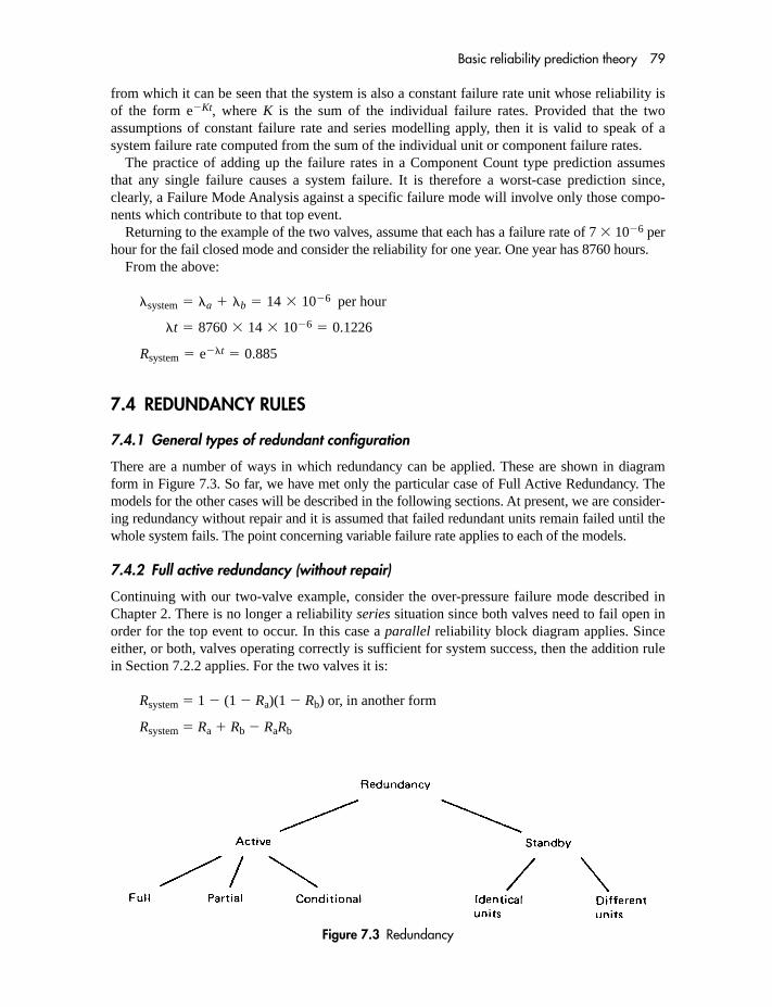
Basic reliability prediction theory 79
from which it can be seen that the system is also a constant failure rate unit whose reliability isof the form e�Kt, where K is the sum of the individual failure rates. Provided that the twoassumptions of constant failure rate and series modelling apply, then it is valid to speak of asystem failure rate computed from the sum of the individual unit or component failure rates.
The practice of adding up the failure rates in a Component Count type prediction assumesthat any single failure causes a system failure. It is therefore a worst-case prediction since,clearly, a Failure Mode Analysis against a specific failure mode will involve only those compo-nents which contribute to that top event.
Returning to the example of the two valves, assume that each has a failure rate of 7 � 10�6 perhour for the fail closed mode and consider the reliability for one year. One year has 8760 hours.
From the above:
7.4 REDUNDANCY RULES
7.4.1 General types of redundant configuration
There are a number of ways in which redundancy can be applied. These are shown in diagramform in Figure 7.3. So far, we have met only the particular case of Full Active Redundancy. Themodels for the other cases will be described in the following sections. At present, we are consider-ing redundancy without repair and it is assumed that failed redundant units remain failed until thewhole system fails. The point concerning variable failure rate applies to each of the models.
7.4.2 Full active redundancy (without repair)
Continuing with our two-valve example, consider the over-pressure failure mode described inChapter 2. There is no longer a reliability series situation since both valves need to fail open inorder for the top event to occur. In this case a parallel reliability block diagram applies. Sinceeither, or both, valves operating correctly is sufficient for system success, then the addition rulein Section 7.2.2 applies. For the two valves it is:
Rsystem � 1 � (1 � Ra)(1 � Rb) or, in another form
Rsystem � Ra � Rb � RaRb
Rsystem � e��t � 0.885
�t � 8760 � 14 � 10�6 � 0.1226
�system � �a � �b � 14 � 10�6 per hour
Figure 7.3 Redundancy

80 Reliability, Maintainability and Risk
In other words, one minus the product of their unreliabilities. Let us assume that the fail openfailure rate of a valve is 3 � 10�6 per hour:
Rsystem � 1 � (0.026)2 �
If there were N items in this redundant configuration such that all may fail except one, then theexpression becomes:
Rsystem � 1 � (1 � Ra)(1 � Rb), . . . , (1 � Rn)
There is a pitfall at this point which it is important to emphasize. The reliability of the sys-tem, after substitution of , becomes:
It is very important to note that, unlike the series case, this combination of constant failurerate units exhibits a reliability characteristic which is not of the form e�Kt. In other words,although constant failure rate units are involved, the failure rate of the system is variable.The MTBF can therefore be obtained only from the integral of reliability. In Chapter 2, wesaw that
Hence
In the above working we substituted � for 1/� which was correct because a unit was beingconsidered for which constant � applies. The danger now is to assume that the failure rate of thesystem is 2�/3. This is not true since the practice of inverting MTBF to obtain failure rate, andvice versa, is valid only for constant failure rate.
Figure 7.4 compares reliability against time, and failure rate against time, for seriesand redundant cases. As can be seen, the failure rate, initially zero, increases asymptotically.Reliability, in a redundant configuration, stays higher than for constant failure rate at thebeginning but eventually falls more sharply. The greater the number of redundant units,the longer the period of higher reliability and the sharper the decline. These features ofredundancy apply, in principle, to all redundant configurations – only the specific valueschange.
� 3�/2 where � is the MTBF of a single unit.
� 3/2�
� 2/� � 1/2�
MTBF � �
0
(2e��t � e�2�t)
MTBF � �
0
R(t) dt
Rs � 2e��t � e�2�t
R � e��t
0.999
e��t � 0.974
Ra � Rb � e��t where �t � 3 � 10�6 � 8760 � 0.026

Basic reliability prediction theory 81
7.4.3 Partial active redundancy (without repair)
Consider three identical units each with reliability R. Let R � Q � 1 so that Q is the unrelia-bility (probability of failure in a given time). The binomial expression (R � Q)3 yields thefollowing terms:
R3, 3R2Q, 3RQ2, Q3 which are
R3, 3R2(1 � R), 3R(1 � R)2, (1 � R)3
This conveniently describes the probabilities of
0, 1, 2, 3 failures of a single unit.
In Section 7.4.2 the reliability for full redundancy was seen to be:
1 � (1 � R)3
This is consistent with the above since it can be seen to be one minus the last term. Since thesum of the terms is unity reliability, it is therefore the sum of the first three terms which, beingthe probability of 0, 1 or 2 failures, is the reliability of a fully redundant system.
In many cases of redundancy, however, the number of units permitted to fail before system fail-ure occurs is less than in full redundancy. In the example of three units, full redundancy requiresonly one to function, whereas partial redundancy would exist if two units were required with onlyone allowed to fail. Once again the reliability can be obtained from the binomial expression sinceit is the probability of 0 or 1 failures which is given by the sum of the first two terms. Hence:
Rsystem � R3 � 3R2(1 � R)
� 3R2 � 2R3
In general, if r items may fail out of n then the reliability is given as the sum of the first r � 1terms of the binomial expansion (R � Q)n. Therefore:
. . . �n(n � 1) . . . (n � r � 1)R n�r(1 � R) r
r!
R � Rn � nR n�1(1 � R) �n(n � 1)R n�2(1 � R)2
2!� . . .
Figure 7.4 Effect of redundancy on reliability and failure rate
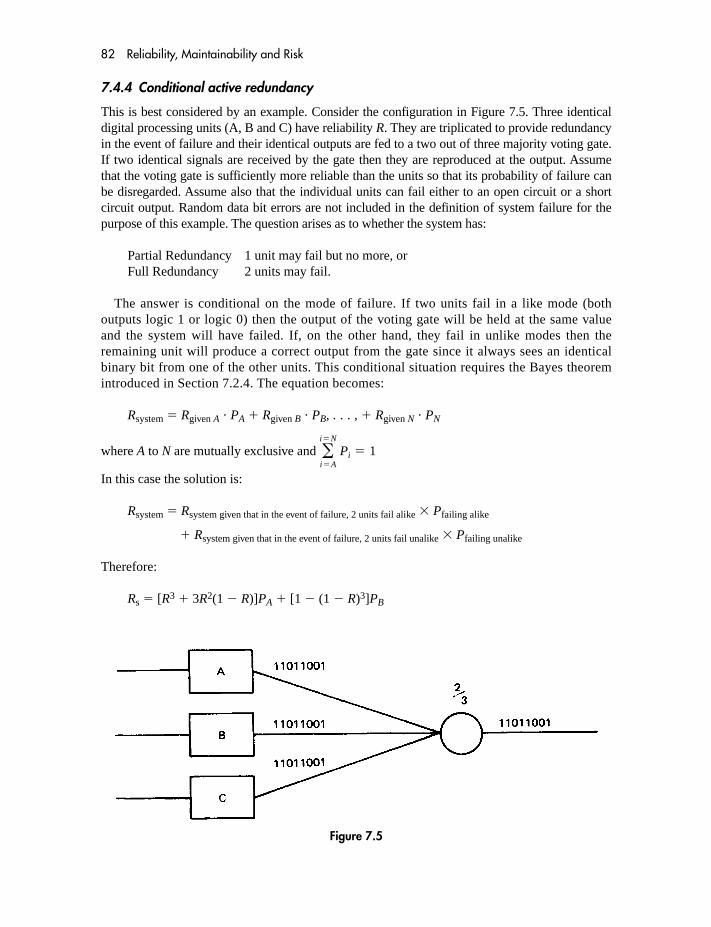
82 Reliability, Maintainability and Risk
7.4.4 Conditional active redundancy
This is best considered by an example. Consider the configuration in Figure 7.5. Three identicaldigital processing units (A, B and C) have reliability R. They are triplicated to provide redundancyin the event of failure and their identical outputs are fed to a two out of three majority voting gate.If two identical signals are received by the gate then they are reproduced at the output. Assumethat the voting gate is sufficiently more reliable than the units so that its probability of failure canbe disregarded. Assume also that the individual units can fail either to an open circuit or a shortcircuit output. Random data bit errors are not included in the definition of system failure for thepurpose of this example. The question arises as to whether the system has:
Partial Redundancy 1 unit may fail but no more, orFull Redundancy 2 units may fail.
The answer is conditional on the mode of failure. If two units fail in a like mode (bothoutputs logic 1 or logic 0) then the output of the voting gate will be held at the same valueand the system will have failed. If, on the other hand, they fail in unlike modes then theremaining unit will produce a correct output from the gate since it always sees an identicalbinary bit from one of the other units. This conditional situation requires the Bayes theoremintroduced in Section 7.2.4. The equation becomes:
Rsystem � Rgiven A � PA � Rgiven B � PB, . . . , � Rgiven N � PN
where A to N are mutually exclusive and
In this case the solution is:
Rsystem � Rsystem given that in the event of failure, 2 units fail alike � Pfailing alike
� Rsystem given that in the event of failure, 2 units fail unalike � Pfailing unalike
Therefore:
Rs � [R3 � 3R2(1 � R)]PA � [1 � (1 � R)3]PB
�i�N
i�A
Pi � 1
Figure 7.5

Basic reliability prediction theory 83
since if two units fail alike there is partial redundancy and if two units fail unalike there is fullredundancy. Assume that the probability of both failure modes is the same and that PA � PB � 0.5.The system reliability is therefore:
7.4.5 Standby redundancy
So far, only active redundancy has been considered where every unit is operating andthe system can function despite the loss of one or more units. Standby redundancyinvolves additional units which are activated only when the operating unit fails. A greaterimprovement, per added unit, is anticipated than with active redundancy since the standbyunits operate for less time. Figure 7.6 shows n identical units with item 1 active. Shoulda failure be detected then item 2 will be switched in its place. Initially, the followingassumptions are made:
1. The means of sensing that a failure has occurred and for switching from the defective to thestandby unit is assumed to be failure free.
2. The standby unit(s) are assumed to have identical, constant failure rates to the main unit.3. The standby units are assumed not to fail while in the idle state.4. As with the earlier calculation of active redundancy, defective units are assumed to remain
so. No repair is effected until the system has failed.
Rs �R3 � 3R2 � 3R3 � 1 � 1 � 3R � 3R2 � R3
2�
3R � R3
2
Figure 7.6

84 Reliability, Maintainability and Risk
Calculations involving redundancy and repair are covered in the next chapter. The reliabilityis then given by the first n terms of the Poisson expression:
which reduces, for two units to:
Figure 7.7 shows the more general case of two units with some of the above assumptionsremoved. In the figure:
�1 is the constant failure rate of the main unit,�2 is the constant failure rate of the standby unit when in use,�3 is the constant failure rate of the standby unit in the idle state,P is the one-shot probability of the switch performing when required.
The reliability is given by:
It remains only to consider the following failure possibilities. Let �4, �5 and �6 be the failurerates associated with the sums of the following failure modes:
For �4 – Dormant failures which inhibit failure sensing or changeover;For �5 – Failures causing the incorrect switching back to the failed unit;For �6 – False sensing of non-existent failure.
If we think about each of these in turn it will be seen that, from the point of view of the above model:
�4 is part of �3�5 is part of �2�6 is part of �1
In the analysis they should therefore be included in the appropriate category.
Rsystem � e��1t �P�1
�2 � �1 � �3 (e�(�1��3)t � e��2t)
Rsystem � e��t(1 � �t)
Rsystem � R(t) � e��t �1 � �t ��2 t2
2! . . . �
(n�1) t (n�1)
(n � 1)! �
Figure 7.7

Basic reliability prediction theory 85
7.4.6 Load sharing
The following situation can be deceptive since, at first sight, it appears as active redundancy.Figure 7.8 shows two capacitors connected in series. Given that both must fail short circuit inorder for the system to fail, we require a model for the system. It is not two units in activeredundant configuration because if the first capacitor should fail (short circuit) then the voltageapplied to the remaining one will be doubled and its failure rate greatly increased. This situa-tion is known as load sharing and is mathematically identical to a standby arrangement.
Figure 7.9 shows two units in standby configuration. The switchover is assumed to beperfect (which is appropriate) and the standby unit has an idle failure rate equal to zero witha different (larger) failure rate after switchover. The main unit has a failure rate of twice thesingle capacitor.
7.5 GENERAL FEATURES OF REDUNDANCY
7.5.1 Incremental improvement
As was seen in Figure 7.4, the improvement resulting from redundancy is not spread evenlyalong the time axis. Since the MTBF is an overall measure obtained by integrating reliabilityfrom zero to infinity, it is actually the area under the curve of reliability against time. For shortmissions (less than one MTBF in duration) the actual improvement in reliability is greater thanwould be suggested simply by comparing MTBFs. For this reason, the length of mission shouldbe taken into account when evaluating redundancy.
As we saw in Section 7.4, the effect of duplicating a unit by active redundancy is to improvethe MTBF by only 50%. This improvement falls off as the number of redundant unitsincreases, as is shown in Figure 7.10. The effect is similar for other redundant configurationssuch as conditional and standby. Beyond a few units the improvement may even be offset bythe unreliability introduced as a result of additional switching and other common mode effectsdealt with in Section 8.2.
Figure 7.8
Figure 7.9

86 Reliability, Maintainability and Risk
Figure 7.10 is not a continuous curve since only the points for integral numbers of units exist.It has been drawn, however, merely to illustrate the diminishing enhancement in MTBF as thenumber of units is increased.
7.5.2 Further comparisons of redundancy
Figure 7.11 shows two alternative configurations involving four units in active redundancy:(i) protects against short-circuit failures (ii) protects against short- and open-circuit conditions.As can be seen from Figure 7.12 (ii) has the higher reliability but is harder to implement.If readers care to calculate the MTBF of (i), they will find that it can be less than for a singleunit and, as can be seen from the curves, the area under the reliability curve (MTBF) is less.It is of value only for conditions where the short-circuit failure mode is more likely.
Figure 7.10
Figure 7.11
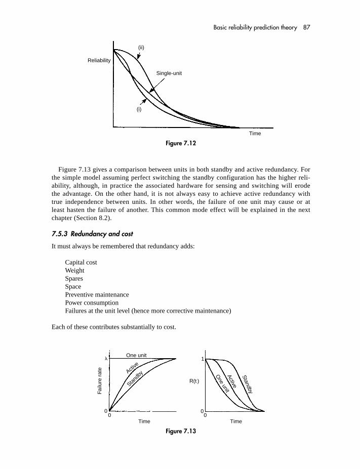
Basic reliability prediction theory 87
Figure 7.13 gives a comparison between units in both standby and active redundancy. Forthe simple model assuming perfect switching the standby configuration has the higher reli-ability, although, in practice the associated hardware for sensing and switching will erodethe advantage. On the other hand, it is not always easy to achieve active redundancy withtrue independence between units. In other words, the failure of one unit may cause or atleast hasten the failure of another. This common mode effect will be explained in the nextchapter (Section 8.2).
7.5.3 Redundancy and cost
It must always be remembered that redundancy adds:
Capital costWeightSparesSpacePreventive maintenancePower consumptionFailures at the unit level (hence more corrective maintenance)
Each of these contributes substantially to cost.
Reliability
(ii)
(i)
Single-unit
Time
Figure 7.12
Failu
re r
ate
Active
Stand
by
One unit
0 0
1
R(t )
0
Time Time
Standby
Active
One unit
0
�
Figure 7.13

88 Reliability, Maintainability and Risk
EXERCISES
1. Provide an expression for the MTBF of the system shown in the following block diagram.
�
�
�
Figure 7.14
2. The following block diagram shows a system whereby unit B may operate with units D or Ebut where unit A may only operate with unit D, or C with E. Derive the reliability expression.
Ra Rb
Re
Rc
Rd
A B C
D E
Figure 7.15

8 Methods of modelling
In Chapter 1 (Section 1.3) and Chapter 7 (Section 7.1) the limitations of reliability of predictionwere emphasized. This chapter describes, in some detail, the available methods.
8.1 BLOCK DIAGRAMS AND REPAIRABLE SYSTEMS
8.1.1 Reliability block diagrams
The following is the general approach to block diagram analysis.
8.1.1.1 Establish failure criteriaDefine what constitutes a system failure since this will determine which failure modes at thecomponent level actually cause a system to fail. There may well be more than one type of sys-tem failure, in which case a number of predictions giving different reliabilities will be required.This step is absolutely essential if the predictions are to have any significance. It was explained,in Section 2.1, how different system failure modes can involve quite different component failuremodes and, indeed, even different series/redundant configurations.
8.1.1.2 Establish a reliability block diagramIt is necessary to describe the system as a number of functional blocks which are interconnectedaccording to the effect of each block failure on the overall system reliability.
Figure 8.1 is a series diagram representing a system of two blocks such that the failure of eitherblock prevents operation of the system. Figure 8.2 shows the situation where both blocks must failin order for the system to fail. This is known as a parallel, or redundancy, case. Figure 8.3 shows a
Figure 8.1
Figure 8.2

90 Reliability, Maintainability and Risk
combination of series and parallel reliability. It represents a system which will fail if block A fails orif both block B and block C fail. The failure of B or C alone is insufficient to cause system failure.
A number of general rules should be borne in mind when defining the blocks.
1. Each block should represent the maximum number of components in order to simplify thediagram.
2. The function of each block should be easily identified.3. Blocks should be mutually independent in that failure in one should not affect the probability
of failure in another (see Section 8.2).4. Blocks should not contain any significant redundancy otherwise the addition of failure rates,
within the block, would not be valid.5. Each replaceable unit should be a whole number of blocks.6. Each block should contain one technology, that is, electronic or electro-mechanical.7. There should be only one environment within a block.
8.1.1.3 Failure mode analysisFailure Mode and Effect Analysis (FMEA) is described later in Chapter 9 (Section 9.3). It providesblock failure rates by examining individual component failure modes and failure rates. Given aconstant failure rate and no internal redundancy, each block will have a failure rate predicted fromthe sum of the failure rates on the FMEA worksheet.
8.1.1.4 Calculation of system reliabilityRelating the block failure rates to the system reliability is a question of mathematical modellingwhich is the subject of the rest of this section. In the event that the system reliability predictionfails to meet the objective then improved failure rate (or down time) objectives must beassigned to each block by means of reliability allocation.
8.1.1.5 Reliability allocationThe importance of reliability allocation is stressed in Chapter 11 and an example is calculated.The block failure rates are taken as a measure of the complexity, and improved, suitablyweighted objectives are set.
8.1.2 Repairable systems (revealed failures)
In Chapter 7, the basic rules for series and redundant systems were explained. For redundantsystems, however, the equations only catered for the case whereby failed redundant units werenot repaired. In other words, the reliability was calculated as the reliability of failure, given thatfailed units stay failed. It is now necessary to address the repairable case.
The traditional approach given in the 6th edition of Reliability Maintainability and Risk,together with the majority of text books and standards, has recently been challenged. It is now
Figure 8.3

Methods of modelling 91
generally acknowledged that the traditional Markov model does not correctly represent thenormal repair activities for redundant repairable systems when calculating the probabilityof failure on demand (PFD). The Journal of The Safety and Reliability Society, Volume 22,No. 2, Summer 2002, published a paper by W. G. (Bill) Gulland, and another by Kenneth G. L.Simpson, both of which agreed with those findings. The rest of this section therefore providesslightly different formulae for repairable systems than were given in previous editions.
The problem arises because repair of multiple failures is not necessarily a Markov Process(namely that the probability of being in a state can be determined solely from knowledge of theprevious state). Hence, Markov modelling gives the correct answer for system failure rate butnot for PFD.
For a redundant repairable system without a dedicated repair crew for each unit, the transi-tion from a multiple failure state to an operating state does not depend on the repair of the lastfailure (as it should for the process to be applicable to a Markov model). In practice, it is relatedto the repair of the previous failure. For this reason a Markov model is pessimistic because itunder-estimates the transition rate from the failed state. It is as if the repair crew abandon theearlier repair (not so in practice) to carry out the repair of the latest failure. With a dedicatedrepair crew per unit then, the repair of the last failure is independent on preceding failures andthe process is approximately Markov with the calculations giving the correct answer. However,real-life situations seldom follow this scenario.
It is worth mentioning that, as with all redundant systems, the total system failure rate (orPFD) will be dominated by the effect of common cause failure (CCF) dealt with in Section 8.2.
For interest, the traditional (incorrect) Markov model is shown in Appendix 13.Coincidentally it does give the correct answer for system failure rate (as mentioned above) ifthe multiple repair crew assumption is used.
The modelling of systems with revealed failures will be carried out here using simple prob-ability rules.
Consider a simple duplicated (one out of two) redundant system. In other words, one unitmust work out of the two for the system to operate. System failure, therefore, requires twofailed units. One can argue as follows:
The failure rate, whereby a given unit fails is, by definition, �. There are, however, twounits and thus the rate for either failing is 2�. For the system to fail it requires that, coinci-dentally, the other unit is in the failed state. This is another way of saying it is Unavailable.Its Unavailability is � MDT (as we saw in Section 2.6 of Chapter 2).Therefore, the system failure rate is 2� � � MDT
� 2�2 MDT
The reader can develop the same argument for units with different failure rates and downtimes to yield
�1�2 (MDT1 � MDT2)
The general expression for m units requiring to operate out of a total of n (with the samefailure rates, �, and mean down times, MDT) becomes:
n!/[(n � m)! (m � 1)!] · �(n�m�1) MDT(n�m)
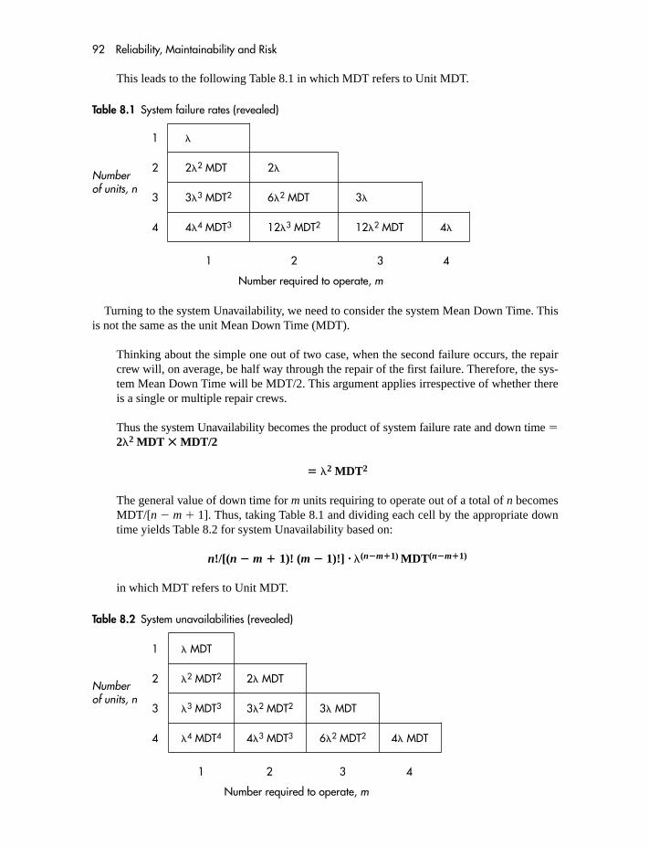
92 Reliability, Maintainability and Risk
This leads to the following Table 8.1 in which MDT refers to Unit MDT.
Turning to the system Unavailability, we need to consider the system Mean Down Time. Thisis not the same as the unit Mean Down Time (MDT).
Thinking about the simple one out of two case, when the second failure occurs, the repaircrew will, on average, be half way through the repair of the first failure. Therefore, the sys-tem Mean Down Time will be MDT/2. This argument applies irrespective of whether thereis a single or multiple repair crews.
Thus the system Unavailability becomes the product of system failure rate and down time �2�2 MDT � MDT/2
� �2 MDT2
The general value of down time for m units requiring to operate out of a total of n becomesMDT/[n � m � 1]. Thus, taking Table 8.1 and dividing each cell by the appropriate downtime yields Table 8.2 for system Unavailability based on:
n!/[(n � m � 1)! (m � 1)!] · �(n�m�1) MDT(n�m�1)
in which MDT refers to Unit MDT.
1 � MDT
2 �2 MDT2 2� MDT
3 �3 MDT3 3�2 MDT2 3� MDT
4 �4 MDT4 4�3 MDT3 6�2 MDT2 4� MDT
1 2 3 4
Number required to operate, m
Numberof units, n
1 �
2 2�2 MDT 2�
3 3�3 MDT2 6�2 MDT 3�
4 4�4 MDT3 12�3 MDT2 12�2 MDT 4�
1 2 3 4
Number required to operate, m
Numberof units, n
Table 8.1 System failure rates (revealed)
Table 8.2 System unavailabilities (revealed)

Methods of modelling 93
The results shown below are independent of the number of repair crews for the reason stated,namely that the repairers of the first failure will continue rather than switch to the second failureand start the MDT again.
8.1.3 Repairable systems (unrevealed failures)
In many cases failures are unrevealed as, for example, the failure of an instrument to measurehigh pressure in a safety-related monitoring system. The pressure may seldom exceed the alarmlimit and thus the inability of the instrument to respond will not be revealed except by someperiodic proof test.
Both unit and system down times will be related to the proof-test interval, T. The followingarguments (similar but different to the revealed failures case) are:
If the system is visited every T hours for the inspection of failed units then the averagedown time AT THE UNIT LEVEL is:
T/2 � Repair Time.
In general, however, the proof-test interval is large compared with the repair time and wemay simplify the above to:
Mean Unit Down Time � T/2
In general the mean time to fail of a unit is much greater than the proof-test interval andso, if z events are needed for the system to fail then these will be evenly distributed acrossthe interval T and, thus, the system will be in failed state for:
Mean System Down Time � T/(z � 1)
For a system where m units are required to operate out of n then n � m � 1 must fail forthe system to fail and so the system down time becomes:
T/(n � m � 2)
The probability of an individual unit failing between proof tests is simply:
� T
For the general m out of n case the probability of the system failing prior to the nextproof test is approximately the same as for the probability of n � m � 1 units failing.This is:
n!/[(m � 1)! (n � m � 1)!] · (�T)(n�m�1)
The failure rate is obtained by dividing the above by T:
n!/[(m � 1)! (n � m � 1)!] · �(n�m�1) · T(n�m)
This yields Table 8.3.

94 Reliability, Maintainability and Risk
The above formulae apply to proof tests which are carried out simultaneously. In otherwords, both of the redundant units are inspected at the same time, every T hours. If the prooftest were to be staggered (e.g. January/July) the Unavailablity would be improved (decreased).The author addressed this issue in a paper in the Safety and Reliability Society Journal,Volume 21, No. 3, Autumn 2001. The result is shown in Table 8.5.
Multiplying these failure rates by the system down time yields Table 8.4.
1 �
2 �2T 2�
3 �3T 2 3�2T 3�
4 �4T 3 4�3T 2 6�2T 4�
1 2 3 4
Number required to operate, m
Numberof units, n
1 �T/2
2 �2T 2/3 �T
3 �3T 3/4 �2T 2 3�T/2
4 �4T4/5 �3T 3 2�2T 2 2�T
1 2 3 4
Number required to operate, m
Numberof units, n
1 �T/2
2 �2T 2/4 �T
3 �3T 3/8 3�2T 2/4 3�T/2
4 �4T4/16 3�3T 3/8 6�2T 2/4 2�T
1 2 3 4
Number required to operate, m
Numberof units, n
Table 8.5 System unavailability (unrevealed – random proof test)
Table 8.3 System failure rates (unrevealed)
Table 8.4 System unavailability (unrevealed)

Methods of modelling 95
8.1.5 Modelling repairable systems with both revealed and unrevealed failures
When carrying out the block diagram modelling it will be necessary to take account of units(e.g. a PLC) which has both revealed and unrevealed failures. Since these attract different for-mulae the approach is to imagine that all the revealed failures are in one hypothetical unit andall the unrevealed failures in another. The parallel block diagram of a one out of two systemwould become as shown in Figure 8.4.
This is addressed in Section 2 of Chapter 9.
revealed unrevealed
Figure 8.4 Model showing revealed and unrevealed failures
Staggered choice of the unit for proof test will lead to yet different results but, this being anunlikely scenario, is not addressed here (an example, for 1 out of 2, is 5�2 T 2/24).
The above results are independent of the number of repair crews.
8.1.4 Systems with cold standby units and repair
Cold standby implies that the redundant units, when not required, are not in use and thus havezero failure rate. Similar logic can be applied to derive expressions for standby scenarioswhereby one redundant unit is not activated until needed. A zero failure rate in the dormantstate is assumed.
In this case the failure rate becomes (n � 1) � because only m � 1 are available to fail. Thefailure rate for the second failure is the same because the standby unit has been activated andis thus (n � 1) �. Thus the probability of the second failure is (n � 1) �. unit down time. Thesystem failure rate is thus:
(n � 1)2 �2 MDTunit
This leads to Table 8.6 for the system unavailabilities.
1 � MDT
2 �2 MDT2/2 2� MDT
3 �3 MDT3/6 2�2 MDT2 3� MDT
4 �4 MDT4/24 4�3 MDT3/3 9�2 MDT2/2 4� MDT
1 2 3 4Number required to operate, m
Numberof units, n
Table 8.6 System unavailability (up to 3 units in standby, i.e. n � 4, m � 1)

96 Reliability, Maintainability and Risk
8.2 COMMON CAUSE (DEPENDENT) FAILURE
8.2.1 What is CCF?
Common cause failures often dominate the unreliability of redundant systems by virtue ofdefeating the random coincident failure feature of redundant protection. Consider the dupli-cated system in Figure 8.5. The failure rate of the redundant element (in other words thecoincident failures) can be calculated using the formula developed in Section 8.1, namely2�2 MDT. Typical figures of 10 per million hours failure rate and 24 hours down time leadto a failure rate of 2 � 10�10 � 24 � 0.0048 per million hours. However, if only one failurein twenty is of such a nature as to affect both channels and thus defeat the redundancy, it isnecessary to add the series element, �2, whose failure rate is 5% � 10�5 � 0.5 per millionhours. The effect is to swamp the redundant part of the prediction. This sensitivity of systemfailure to CCF places emphasis on the credibility of CCF estimation and thus justifies effortsto improve the models.
Whereas simple models of redundancy (developed in Section 8.1) assume that failures areboth random and independent, common cause failure (CCF) modelling takes account of failureswhich are linked, due to some dependency, and therefore occur simultaneously or, at least,within a sufficiently short interval as to be perceived as simultaneous.
Two examples are:
(a) the presence of water vapour in gas causing both valves in twin streams to seize due toicing. In this case the interval between the two failures might be in the order of days.However, if the proof-test interval for this dormant failure is two weeks then the two fail-ures will, to all intents and purposes, be simultaneous.
(b) inadequately rated rectifying diodes on identical twin printed circuit boards failing simultan-eously due to a voltage transient.
Typically, causes arise from:
(a) Requirements: Incomplete or conflicting(b) Design: Common power supplies, software, emc, noise(c) Manufacturing: Batch-related component deficiencies(d) Maintenance/Operations: Human induced or test equipment problems(e) Environment: Temperature cycling, electrical interference, etc.
�1
�2
�1
Figure 8.5 Reliability block diagrams for CCF

Methods of modelling 97
Defences against CCF involve design and operating features which form the assessmentcriteria shown in the next section.
The term common mode failure (CMF) is also frequently used and a brief explanation ofthe difference between CMF and CCF is therefore necessary. Common mode failure refersto coincident failures of the same mode, in other words failures which have an identicalappearance or effect. On the other hand, the term CCF implies that the failures have thesame underlying cause. It is possible (although infrequent) for two CMFs not to have acommon cause and, conversely, for two CCFs not to manifest themselves in the same mode.In practice the difference is slight and unlikely to affect the data, which rarely containsufficient detail to justify any difference in the modelling. Since the models described in thissection involve assessing defences against the CAUSES of coincident failure, CCF will beused throughout.
8.2.2 Types of CCF model
Various approaches to modelling are:
(a) The simple BETA (�) model, which assumes that a fixed proportion (�) of the failures arisefrom a common cause. The estimation of (�) is assessed according to the system. (Note theBeta used in this context has no connection with the shape parameter used in the Weibullmethod, Chapter 6.) The method is based on very limited historical data.
In Figure 8.5 (�1) is the failure rate of a single redundant unit and (�2) is the commoncause failure rate such that for the simple BETA model and also the PartialBETA model, in (b) below.
(b) The Partial BETA model, also assumes that a fixed proportion of the failures arise from acommon cause. It is more sophisticated than the simple BETA model in that the contribu-tions to BETA are split into groups of design and operating features which are believed toinfluence the degree of CCF. Thus the BETA factor is made up by adding together thecontributions from each of a number of factors within each group. In traditional PartialBETA models the following groups of factors, which represent defences against CCF, canbe found:– Similarity (Diversity between redundant units reduces CCF)– Separation (Physical distance and barriers reduce CCF)– Complexity (Simpler equipment is less prone to CCF)– Analysis (Previous FMEA and field data analysis will have reduced CCF)– Procedures (Control of modifications and of maintenance activities can reduce CCF)– Training (Designers and maintainers can help to reduce CCF by understanding root causes)– Control (Environmental controls can reduce susceptibility to CCF, e.g. weather proofing
of duplicated instruments)– Tests (Environmental tests can remove CCF prone features of the design, e.g. emc testing)The Partial BETA model is also represented by the reliability block diagram shown inFigure 8.5. BETA is assumed to be made up of a number of partial �s, each contributed toby the various groups of causes of CCF. � is then estimated by reviewing and scoring eachof the contributing factors (e.g. diversity, separation).
(c) The System Cut-off model offers a single failure rate for all failures (independent anddependent both combined). It argues that the dependent failure rate dominates the coinci-dent failures. Again, the choice is affected by system features such as diversity and separa-tion. It is the least sophisticated of the models in that it does not base the estimate of systemfailure rate on the failure rate of the redundant units.
(�2) � �(�1)

98 Reliability, Maintainability and Risk
(d) The Boundary model uses two limits of failure rate. Namely, limit A which assumes all failuresare common cause (�u) and limit B which assumes all failures are random (�1). The systemfailure rate is computed using a model of the following type:
where the value of n is chosen according to the degree of diversity between the redundantunits. n is an integer, normally from 0 to 4, which increases with the level of diversitybetween redundant units. It is chosen in an arbitrary and subjective way. This method is amathematical device, having no foundation in empirical data, which relies on a subjectiveassessment of the value of n. It provides no traceable link (as does the Partial BETA method)between the assessment of n and the perceived causes of CCF. Typical values of n for dif-ferent types of system are:
Configuration Mode of Precautions against CCF noperation
Redundant equipment/system Parallel No segregation of services or supplies 0Redundant equipment/system Parallel Full segregation of services or supplies 1Redundant equipment/system Duty/standby No segregation of services or supplies 1Redundant equipment/system Duty/standby Full segregation of services or supplies 2Diverse equipment or system Parallel No segregation of services or supplies 2Diverse equipment or system Parallel Full segregation of services or supplies 3Diverse equipment or system Duty/standby No segregation of services or supplies 3Diverse equipment or system Duty/standby Full segregation of services or supplies 4
(e) The Multiple Greek Letter model is similar to the BETA model but assumes that the BETAratio varies according to the number of coincident failures. Thus two coincident failures andthree coincident failures would have different BETAs. However, in view of the inaccuracyinherent in the approximate nature of these models it is considered to be too sophisticatedand cannot therefore be supported by field data until more detailed information is available.
All the models are, in their nature, approximate but because CCF failure rates (which are inthe order of ) are much greater than the coincident independent failures (in the order of ),then greater precision in estimating CCF is needed than for the redundant coincident modelsdescribed in Section 8.1.
8.2.3 The BETAPLUS model
The BETAPLUS model has been developed from the Partial BETA method, by the author, because:
– it is objective and maximizes traceability in the estimation of BETA. In other words thechoice of checklist scores when assessing the design, can be recorded and reviewed.
– it is possible for any user of the model to develop the checklists further to take account ofany relevant failure causal factors that may be perceived.
�n� �
� � (�n1 �u)1/(n�1)

Methods of modelling 99
– it is possible to calibrate the model against actual failure rates, albeit with very limited data.– there is a credible relationship between the checklists and the system features being analysed.
The method is thus likely to be acceptable to the non-specialist.– the additive scoring method allows the partial contributors to � to be weighted separately.– the � method acknowledges a direct relationship between (�2) and (�1) as depicted in
Figure 8.5.– it permits an assumed ‘non-linearity’ between the value of � and the scoring over the range of �.
The Partial BETA model includes the following enhancements:
(a) CATEGORIES OF FACTORS:Whereas existing methods rely on a single subjective judgement of score in each category,the BETAPLUS method provides specific design and operational related questions to beanswered in each category. Specific questions are individually scored, in each category(i.e. separation, diversity, complexity, assessment, procedures, competence, environmentalcontrol, environmental test) thereby permitting an assessment of the design and its operat-ing and environmental factors. Other BETA methods only involve a single scoring of eachcategory (e.g. a single subjective score for diversity).
(b) SCORING:The maximum score for each question has been weighted by calibrating the results ofassessments against known field operational data. Programmable and non-programmableequipment have been accorded slightly different checklists in order to reflect the equipmenttypes (see Appendix 10).
(c) TAKING ACCOUNT OF DIAGNOSTIC COVERAGE:Since CCF are not simultaneous, an increase in auto-test or proof-test frequency will reduce� since the failures may not occur at precisely the same moment. Thus, more frequent test-ing will prevent some CCF. Some defences will protect against the type of failure whichincreased proof test might identify (for example failures in parallel channels where diversitywould be beneficial). Other defences will protect against the type of failure which increasedproof test is unlikely to identify (for example failures prevented as a result of long-termexperience with the type of equipment) and this is reflected in the model.
(d) SUB-DIVIDING THE CHECKLISTS ACCORDING TO THE EFFECT OF DIAGNOSTICS:Two columns are used for the checklist scores. Column (A) contains the scores for those fea-tures of CCF protection which are perceived as being enhanced by an increase of diagnosticfrequency (either proof-test or auto-test). Column (B), however, contains the scores for thosefeatures thought not to be enhanced by an improvement in diagnostic frequency. In somecases the score has been split between the two columns, where it is thought that some, butnot all, aspects of the feature are affected.
(e) ESTABLISHING A MODEL:The model allows the scoring to be modified by the frequency and coverage of diagnostic test.The (A) column scores are modified by multiplying by a factor (C) derived from diagnosticrelated considerations. This (C) score is based on the diagnostic frequency and coverage. (C) isin the range 1–3. BETA is then estimated from the following RAW SCORE total:
S � RAW SCORE � (A C) � B
It is assumed that the effect of the diagnostic score (C) on the effectiveness of the (A) featuresis linear. In other words each failure mode is assumed to be equally likely to be revealed bythe diagnostics. Only more detailed data can establish if this is not a valid assumption.

100 Reliability, Maintainability and Risk
(f) NON-LINEARITY:There are currently no CCF data to justify departing from the assumption that, as BETAdecreases (i.e. improves) then successive improvements become proportionately harder toachieve. Thus the relationship of the BETA factor to the raw score [(A C) � B] is assumedto be exponential and this non-linearity is reflected in the equation which translates the rawscore into a BETA factor.
(g) EQUIPMENT TYPE:The scoring has been developed separately for programmable and non-programmableequipment, in order to reflect the slightly different criteria which apply to each type ofequipment.
(h) CALIBRATION:The model was calibrated against the author’s field data.
8.2.3.1 Checklists and scoring of the (A) and (B) factors in the modelScoring criteria were developed to cover each of the categories (i.e. separation, diversity, complex-ity, assessment, procedures, competence, environmental control, environmental test). Questionshave been assembled to reflect the likely features which defend against CCF. The scores were thenadjusted to take account of the relative contributions to CCF in each area, as shown in the author’sdata. The score values have been weighted to calibrate the model against the data.
When addressing each question a score, less than the maximum of 100% may be entered. Forexample, in the first question, if the judgement is that only 50% of the cables are separated then50% of the maximum scores (15 and 52) may be entered in each of the (A) and (B) columns(7.5 and 26).
The checklists are presented in two forms (see Appendix 10) because the questions applic-able to programmable based equipments will be slightly different to those necessary for non-programmable items (e.g. field devices and instrumentation).
The headings (expanded with scores in Appendix 10) are:
(1) SEPARATION/SEGREGATION(2) DIVERSITY/REDUNDANCY(3) COMPLEXITY/DESIGN/APPLICATION/MATURITY/EXPERIENCE(4) ASSESSMENT/ANALYSIS and FEEDBACK of DATA(5) PROCEDURES/HUMAN INTERFACE(6) COMPETENCE/TRAINING/SAFETY CULTURE(7) ENVIRONMENTAL CONTROL(8) ENVIRONMENTAL TESTING
8.2.3.2 Assessment of the diagnostic interval factor (C)In order to establish the (C) score it is necessary to address the effect of the frequency andcoverage of proof test or auto-test. The diagnostic coverage, expressed as a percentage, is anestimate of the proportion of failures which would be detected by the proof test or auto-test.This can be estimated by judgement or, more formally, by applying FMEA at the componentlevel to decide whether each failure would be revealed by the diagnostics. Appendix 10 showsthe detailed scoring criteria.
An exponential model is proposed to reflect the increasing difficulty in further reducingBETA as the score increases (as discussed in paragraph 8.2.3.f). This is reflected in the follow-ing equation:
� � 0.3 exp (�3.4S/2624)

Methods of modelling 101
Because of the nature of this model, additional features (as perceived by any user) can beproposed in each of the categories. The model can then be modified. If subsequent field dataindicate a change of relative importance between the categories then adjust the scores in eachcategory so that the category totals reflect the new proportions, also ensuring that the totalpossible raw score (S � 2624) remains unaltered.
The model can best be used iteratively to test the effect of design, operating and maintenanceproposals where these would alter the scoring. A BETA value can be assessed for a proposedequipment. Proposed changes can be reflected by altering the scores and recalculating BETA.The increased design or maintenance cost can be reviewed against the costs and/or savings inunavailability by re-running the RAMS predictions using the improved BETA. As with allRAMS predictions the proportional comparison of values rather than the absolute value is ofprimary value.
8.3 FAULT TREE ANALYSIS
8.3.1 The Fault Tree
A Fault Tree is a graphical method of describing the combinations of events leading to a definedsystem failure. In fault tree terminology, the system failure mode is known as the top event.
The fault tree involves essentially three logical possibilities and hence two main symbols.These involve gates such that the inputs below gates represent failures. Outputs (at the top) ofgates represent a propagation of failure depending on the nature of the gate. The three types are:
The OR gate whereby any input causes the output to occur;The AND gate whereby all inputs need to occur for the output to occur;The voted gate, similar to the AND gate, whereby two or more inputs are needed for theoutput to occur.
Figure 8.6 shows the symbols for the AND and OR gates and also draws attention to theirequivalence to reliability block diagrams. The AND gate models the redundant case and is thusequivalent to the parallel block diagram. The OR gate models the series case whereby any fail-ure causes the top event. An example of a voted gate is shown in Figure 8.10.
Figure 8.6

102 Reliability, Maintainability and Risk
For simple trees the same equations given in Section 8.1 on reliability block diagrams can beused and the difference is merely in the graphical method of modelling. In probability terms theAND gate involves multiplying probabilities of failure and the OR gate the addition rules givenin Chapter 7. Whereas reliability block diagrams model paths of success, the fault tree modelsthe paths of failure to the top event.
A fault tree is constructed as shown in Figure 8.7 in which two additional symbols can beseen. The rectangular box serves as a place for the description of the gate below it. Circles,always at the furthest point down any route, represent the basic events which serve as theenabling inputs to the tree.
8.3.2 Calculations
Having modelled the failure logic, for a system, as a fault tree the next step is to evaluatethe frequency of the top event. As with block diagram analysis, this can be performed,for simple trees, using the formulae from Section 8.1. More complex trees will be con-sidered later.
Figure 8.7

Methods of modelling 103
The example shown in Figure 8.7 could be evaluated as follows. Assume the following basicevent data:
Failure rate (PMH) MDT (hours)
PSU 100 24Standby 500 168Motor 50 168Detector 5 168Panel 10 24Pump 60 24
The failure rate ‘outputs’ of AND gates G2 and G3 can be obtained from the formula �1 � �2 �(MDT1 � MDT2). Where an AND gate is actually a voted gate, as, for example, two out ofthree, then again the formulae from Section 8.1 can be used. The outputs of the OR gates G1 andGTOP can be obtained by adding the failure rates of the inputs. Figure 8.8 has the failure rateand MDT values shown.
Figure 8.8
� = 120 MTBF = 0.95 yrsMDT = 84 hours Av = 0.01
Pump � = 60
MDT = 24 hours
G2� = 0.0096
MDT = 21 hours
G3� = 9.6
MDT = 21 hours
PSU� = 100
MDT = 24 hours
Standby� = 500
MDT = 168 hours
G1� = 59.6
MDT = 144 hours
Panel� = 10
MDT = 24 hours
UV� = 5
MDT = 168 hours
Motor� = 50
MDT = 168 hours
G1
GTOP
G2
G3

104 Reliability, Maintainability and Risk
It often arises that the output of an OR gate serves as an input to another gate. In this casethe MDT associated with the input would be needed for the equation. If the MDTs of thetwo inputs to the lower gate are not identical then it is necessary to compute an equivalentMDT. In Figure 8.8 this has been done for G1 even though the equivalent MDT is notneeded elsewhere. It is the weighted average of the two MDTs weighted by failure rate. Inthis case,
In the case of an AND gate it can be shown that the resulting MDT is obtained from the mul-tiple of the individual MDTs divided by their sum. Thus for G3 the result becomes
8.3.3 Cutsets
A problem arises, however, in evaluating more complex trees where the same basic initiatingevent occurs in more than one place. Using the above formulae, as has been done for Figure 8.8,would lead to inaccuracies because an event may occur in more than one Cutset. A Cutset isthe name given to each of the combinations of base events which can cause the top event. In theexample of Figure 8.7 the cutsets are:
PumpMotorPanel and detectorPSU and standby
The first two are referred to as First-Order Cutsets since they involve only single events whichalone trigger the top event. The remaining two are known as Second-Order Cutsets becausethey are pairs of events. There are no third- or higher-order Cutsets in this example. The relativefrequency of cutsets is of interest and this is addressed in the next section.
8.3.4 Computer tools
Manually evaluating complex trees, particularly with basic events which occur more than once,is not easy and would be time consuming. Fortunately, with the recent rapid increase in com-puter (PC) speed and memory capacity, a large number of software packages (such as TTREE)have become available for fault tree analysis. They are quite user-friendly and the degree ofcompetition ensures that efforts continue to enhance the various packages, in terms of facilitiesand user-friendliness.
The majority of packages are sufficiently simple to use that even the example in Figure 8.7would be considerably quicker by computer. The time taken to draw the tree manually wouldexceed that needed to input the necessary logic and failure rate data to the package. There aretwo methods of inputting the tree logic:
(24 � 168)
(24 � 168)� 21 h
(21 � 9.6) � (168 � 50)
(9.6 � 50)� 144 h

Methods of modelling 105
1. Gate logic which is best described by writing the gate logic for Figure 8.7 as follows:
GTOP � G1 G2 PUMPG1 � G3 MOTORG3 * PSU STANDBYG2 * DETECT PANEL
� represents an OR gate and * an AND gate. Each gate, declared on the right-hand side,subsequently appears on the left-hand side until all gates have been described in terms of allthe basic events on the right. Modern packages are capable of identifying an illogical tree.Thus, gates which remain undescribed or are unreachable will cause the program to reportan error.
2. A graphical tree, which is constructed on the PC screen by use of cursors or a mouse to pickup standard gate symbols and to assemble them into an appropriate tree.
Failure rate and mean down-time data are then requested for each of the basic events. Theoption exists to describe an event by a fixed probability as an alternative to stating a rate anddown time. This enables fault trees to contain ‘one-shot’ events such as lightning and humanerror.
Most computer packages reduce the tree to Cutsets (known as minimal Cutsets) which arethen quantified. Some packages compute by the simulation technique described in Section 9.5.
The outputs consist of:
GRAPHICS TO A PLOTTER OR PRINTER (e.g. Figures 8.7, 8.9, 8.10)MTBF, AVAILABILITY, RATE (for the top event and for individual Cutsets)RANKED CUTSETSIMPORTANCE MEASURES
Cutset ranking involves listing the Cutsets in ranked order of one of the variables of interest – say,Failure Rate. In Figure 8.8 the Cutset whose failure rate contributes most to the top event is thePUMP (50%). The least contribution is from the combined failure of UV DETECTOR andPANEL. The ranking of Cutsets is thus:
PUMP (50%)MOTOR (40%)PSU and STANDBY (8%)UV DETECTOR and PANEL (Negligible)
There are various applications of the importance concept but, in general, they involve ascribing anumber either to the basic events or to Cutsets which describes the extent to which they contributeto the top event. In the example, the PUMP MTBF is 1.9 years whereas the overall top eventMTBF is 0.95 year. Its contribution to the overall failure rate is thus 50%. An importance measureof 50% is one way of describing the PUMP either as a basic event or, as is the case here, a Cutset.
If the cutsets were to be ranked in order of Unavailability the picture might be different, sincethe down times are not all the same. In Exercise 3, at the end of Chapter 9, the reader can comparethe ranking by Unavailability with the above ranking by failure rate.
An extract from a typical cutset ranking (taken from the Technis TTREE computer package – seeend of book) is shown below.

106 Reliability, Maintainability and Risk
Barlow-Proschan measure of cutset importance
Rank 1 Importance 0.353 MTBF hours 0.283E�08 MTBF years 0.323E�04
Basic Type Failure Mean Fault ConstantEvent Rate Duration ProbabilityFLANGE I/E 0.180E�03 20.0 (MDT)HE1 E 0.100E�01CPU I/E 0.500E�05 0.800E�04 (PTI)
Rank 2 Importance 0.179 MTBF hours 0.558E�08 MTBF years 0.636E�04
Basic Type Failure Mean Fault ConstantEvent Rate Duration ProbabilityFLANGE I/E 0.180E�03 20.0 (MDT)HE1 E 0.100E�01HE2 E 0.100E�01
Rank 3 Importance 0.110 MTBF hours 0.905E�08 MTBF years 0.103E�05
Basic Type Failure Mean Fault ConstantEvent Rate Duration ProbabilityFLANGE I/E 0.180E�03 20.0 (MDT)CCF1 I/E 0.780E�06 0.800E�04 (PTI)CPU I/E 0.500E�05 0.800E�04 (PTI)
Rank 4 Importance 0.574E�01 MTBF hours 0.174E�09 MTBF years 0.199E�05
Basic Type Failure Mean Fault ConstantEvent Rate Duration ProbabilityFLANGE I/E 0.180E�03 20.0 (MDT)HE1 E 0.100E�01CCF3 I/E 0.800E�06 0.800E�04 (PTI)
The names Barlow–Proschan refer to the fact that the cutsets are ranked in order of MTBF(rather than Unavailability). Ranking by Unavailability is referred to by the names Fussell–Vesely.It can be seen that the first three cutsets account for 64.2% (i.e. 35.3% � 17.9% � 11%) of thetotal failure rate. Note, also, that the event ‘flange’ is common to all three. Thus, suggestions forimproving the reliability will take account of this. It can also be seen that the next (4th) cutset hasan importance of only 5.7%. This tells us that from the 4th cutset downwards, no one cutset isparticularly significant. One other point to note is the column for down time which (in the TTREEpackage) distinguishes between revealed failures, having a mean down time (MDT), and unre-velead failures, subject to a proof-test interval (PTI).
8.3.5 Allowing for CCF
Figure 8.9 shows the reliability block diagram of Figure 8.5 in fault tree form. The commoncause failure can be seen to defeat the redundancy by introducing an OR gate above theredundant G1 gate.
Figure 8.10 shows another example, this time of two out of three redundancy, where a votedgate is used.

Methods of modelling 107
Lambda 1Second item
BA
Lambda 1First item
GTOP
Redundantpair
Lambda 2Common cause
failure
G1 CCF
Topevent
Figure 8.9
CB
2/3G1
A
Topevent
Lambda 1Second item
Lambda 1Third item
Lambda 1First item
GTOP
Lambda 2Common cause
failure
2 out of 3redundancy
CCF
Figure 8.10
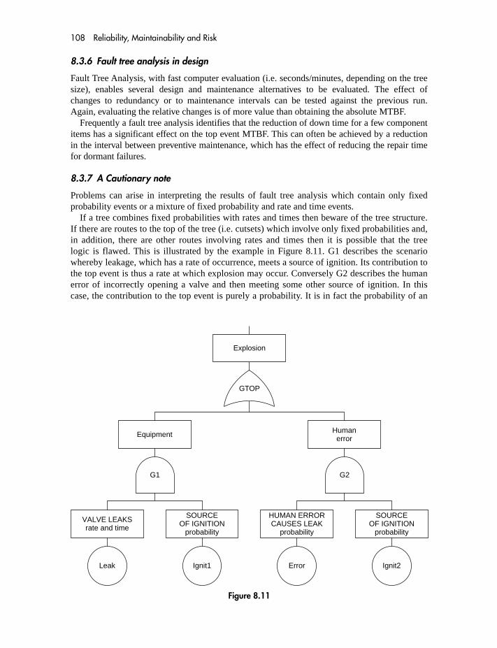
108 Reliability, Maintainability and Risk
8.3.6 Fault tree analysis in design
Fault Tree Analysis, with fast computer evaluation (i.e. seconds/minutes, depending on the treesize), enables several design and maintenance alternatives to be evaluated. The effect ofchanges to redundancy or to maintenance intervals can be tested against the previous run.Again, evaluating the relative changes is of more value than obtaining the absolute MTBF.
Frequently a fault tree analysis identifies that the reduction of down time for a few componentitems has a significant effect on the top event MTBF. This can often be achieved by a reductionin the interval between preventive maintenance, which has the effect of reducing the repair timefor dormant failures.
8.3.7 A Cautionary note
Problems can arise in interpreting the results of fault tree analysis which contain only fixedprobability events or a mixture of fixed probability and rate and time events.
If a tree combines fixed probabilities with rates and times then beware of the tree structure.If there are routes to the top of the tree (i.e. cutsets) which involve only fixed probabilities and,in addition, there are other routes involving rates and times then it is possible that the treelogic is flawed. This is illustrated by the example in Figure 8.11. G1 describes the scenariowhereby leakage, which has a rate of occurrence, meets a source of ignition. Its contribution tothe top event is thus a rate at which explosion may occur. Conversely G2 describes the humanerror of incorrectly opening a valve and then meeting some other source of ignition. In thiscase, the contribution to the top event is purely a probability. It is in fact the probability of an
Ignit2Error
Explosion
GTOP
G2
Equipment Humanerror
G1
Ignit1Leak
VALVE LEAKSrate and time
SOURCEOF IGNITION
probability
SOURCEOF IGNITION
probability
HUMAN ERRORCAUSES LEAK
probability
Figure 8.11
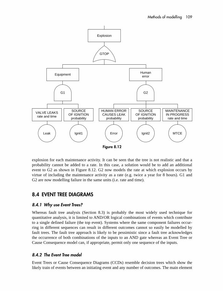
Methods of modelling 109
explosion for each maintenance activity. It can be seen that the tree is not realistic and that aprobability cannot be added to a rate. In this case, a solution would be to add an additionalevent to G2 as shown in Figure 8.12. G2 now models the rate at which explosion occurs byvirtue of including the maintenance activity as a rate (e.g. twice a year for 8 hours). G1 andG2 are now modelling failure in the same units (i.e. rate and time).
8.4 EVENT TREE DIAGRAMS
8.4.1 Why use Event Trees?
Whereas fault tree analysis (Section 8.3) is probably the most widely used technique forquantitative analysis, it is limited to AND/OR logical combinations of events which contributeto a single defined failure (the top event). Systems where the same component failures occur-ring in different sequences can result in different outcomes cannot so easily be modelled byfault trees. The fault tree approach is likely to be pessimistic since a fault tree acknowledgesthe occurrence of both combinations of the inputs to an AND gate whereas an Event Tree orCause Consequence model can, if appropriate, permit only one sequence of the inputs.
8.4.2 The Event Tree model
Event Trees or Cause Consequence Diagrams (CCDs) resemble decision trees which show thelikely train of events between an initiating event and any number of outcomes. The main element
MTCEErrorIgnit1Leak Ignit2
MAINTENANCEIN PROGRESSrate and time
GTOP
G2
Equipment Humanerror
G1
VALVE LEAKSrate and time
SOURCEOF IGNITION
probability
SOURCEOF IGNITION
probability
HUMAN ERRORCAUSES LEAK
probability
Explosion
Figure 8.12

110 Reliability, Maintainability and Risk
in a CCD is the decision box which contains a question/condition with YES/NO outcomes. Theoptions are connected by paths, either to other decision boxes or to outcomes. Comment boxescan be added at any stage in order to enhance the clarity of the model.
Using a simple example the equivalence of fault tree and event tree analysis can be demon-strated. Figures 8.13 and 8.14 compare the fault tree AND and OR logic cases with theirequivalent CCD diagrams. In both cases there is only one Cutset in the fault tree.
Figure 8.14(a) Pump 1 and 2Figure 8.14(b) Smoke Detector or Alarm Bell
These correspond to the ‘system fails’ and ‘no alarm’ paths through the CCD diagrams inFigures 8.14(a) and (b) respectively.
Simple CCDs, with no feedback (explained later) can often be modelled using equivalentfault trees but in cases of sequential operation, the CCD may be easier to perceive.
Figure 8.13
Figure 8.14

Methods of modelling 111
8.4.3 Quantification
A simple event tree, with no feedback loops, can be evaluated by simple multiplication ofYES/NO probabilities where combined activities are modelled through the various paths.
Figure 8.15 shows the Fire Water Deluge example using a pump failure rate of 50 per millionhours with a mean down time of 50 hours. The unavailability of each pump is thus obtainedfrom:
50 � 10�6 � 50 � 0.0025
The probability of a pump not being available on demand is thus 0.0025 and the probabilities ofboth 100% system failure and 50% capacity on demand are calculated.
The system fail route involves the square of 0.0025. The 50% capacity route involvestwo ingredients of 0.0025 � 0.9975. The satisfactory outcome is, therefore, the square of0.9975.
8.4.4 Differences
The main difference between the two models (fault tree and event tree) is that the event treemodels the order in which the elements fail. For systems involving sequential operation it maywell be easier to model the failure possibilities by event tree rather than to attempt a fault tree.
In the above example the event tree actually evaluated two possible outcomes instead of thesingle outcome (no deluge water) in the corresponding fault tree. As was seen in the example,the probabilities of each outcome were required and were derived from the failure rate anddown time of each event.
Figure 8.15

112 Reliability, Maintainability and Risk
The following table summarizes the main differences between Event Tree and Fault Treemodels.
Cause Consequence Fault Tree
Easier to follow for non-specialist Less obvious logicPermits several outcomes Permits one top eventPermits sequential events Static logic (implies sequence is irrelevant)Permits intuitive exploration of outcomes Top-down model requires inferencePermits feedback (e.g. waiting states) No feedbackFixed probabilities Fixed probabilities and rates and times
8.4.5 Feedback loops
There is a complication which renders event trees difficult to evaluate manually. In the examplesquoted so far, the exit decisions from each box have not been permitted to revisit existing boxes.In that case the simple multiplication of probabilities is not adequate.
Feedback loops are required for continuous processes or where a waiting process appliessuch that an outcome is reached only when some set of circumstances arises. Figure 8.16shows a case where a feedback loop is needed where it is necessary to model the situationthat a flammable liquid may or may not ignite before the relief valve closes. Either numericalintegration or simulation (Section 9.5) is needed to quantify this model and a PC computersolution is preferred.
Figure 8.16

9 Quantifying the reliability models
9.1 THE RELIABILITY PREDICTION METHOD
This section summarizes how the methods described in Chapters 8 and 9 are brought togetherto quantify RAMS, and Figure 9.1 gives an overall picture of the prediction process. It hasalready been emphasized that each specific system failure mode has to be addressed separatelyand thus targets are required for each mode (or top event in fault tree terminology). Predictionrequires the choice of suitable failure rate data and this has been dealt with in detail in Chapter 4.Down times also need to be assessed and it will be shown, in Section 9.2, how repair timesand diagnostic intervals both contribute to the down time. The probability of human error(Section 9.4) may also need to be assessed where fault trees or event trees contain human events(e.g. operator fails to act following an alarm).
One or more of the modelling techniques described in Chapter 8 will have been chosen forthe scenario. The choice between block diagram and fault tree modelling is very much a matterfor the analyst and will depend upon:
– which technique he/she favours– what tools are available (i.e. FTA program)– the complexity of the system to be modelled– the most appropriate graphical representation of the failure logic
Chapter 8 showed how to evaluate the model in terms of random coincident failures.Common cause failures then need to be assessed as were shown in Section 8.2. These can beadded into the models either as:
– series elements in the reliability block diagrams (Section 8.1)– OR gates in the fault trees (Section 8.3.5)
Traditionally this process will provide a single predicted RAMS figure. However, the workdescribed in Section 4.4 allows the possibility of expressing the prediction as a confidencerange and showed how to establish the confidence range for mixed data sources. Section 9.6shows how comparisons with the original targets might be made.
Figure 9.1 also reminds us that the opportunity exists to revise the targets should they befound to be unrealistic. It also emphasizes that the credibility of the whole process is dependenton field data being collected to update the data sources being used. The following sectionsaddress specific items which need to be quantified.

114 Reliability, Maintainability and Risk
9.2 ALLOWING FOR DIAGNOSTIC INTERVALS
We saw, in Section 8.1.3, how the down time of unrevealed failures could be assessed.Essentially it is obtained from a fraction of the proof-test interval (i.e. half, at the unit level) aswell as the MTTR (mean time to repair).
Some data bases include information about MTTRs and those that do have been indicated inSection 4.2.
Createreliability model
Assess randomcoincident failures
Assess commoncause failures
Maintenancee.g. spares,
intervals,crews, etc.
Down times
Human error
Environmentand operating conditions
RAMSTargets
for each system failure
Address eachfailure mode separately
Choosefailure
rate data
Predicted reliability rangemin max
Compare withRAMS Target
Implement design
Field data
RAMSALARP?optimum LCC?
Analyse data toenhance data bank
and demonstrate RAMS
Modify design Modify targetsNo No
Yes
(Possible path)
LCC = Life-cycle cost
Figure 9.1

Quantifying the reliability models 115
In many cases there is both auto-test, whereby a programmable element in the system carriesout diagnostic checks to discover unrevealed failures, as well as a manual proof test. In practicethe auto-test will take place at some relatively short interval (e.g. 8 minutes) and the proof testat a longer interval (e.g. 4000 h).
The question arises as to how the reliability model takes account of the fact that failuresrevealed by the auto-test enjoy a shorter down time than those left for the proof test. The ratioof one to the other is a measure of the diagnostic coverage and is expressed as a percentage offailures revealed by the test.
Diagnostic coverage targets frequently quoted are 60%, 90% and 99% (e.g. in the IEC 61508functional safety standard). At first this might seem a realistic range of diagnostic capabilityranging from simple to comprehensive. However, it is worth considering how the existence ofeach of these coverages might be established. There are two ways in which diagnostic coveragecan be assessed:
1. By test: In other words failures are simulated and the number of diagnosed failures counted.2. By FMEA: In other words the circuit is examined (by FMEA described in Section 9.3)
ascertaining, for each potential component failure mode, whether it would be revealed bythe diagnostic program.
Clearly a 60% diagnostic could be demonstrated fairly easily by either method. Test would requirea sample of only a few failures to reveal 60% or alternatively a ‘broad brush’ FMEA, addressingblocks of circuitry rather than individual components, would establish in an hour or two if 60% isachieved. Turning to 90% coverage, the test sample would now need to exceed 20 failures and theFMEA would require a component level approach. In both cases the cost and time begin tobecome onerous. For 99% coverage the sample size would now exceed 200 failures and this islikely to be impracticable. The alternative FMEA approach shown in Section 9.3 would beextremely onerous and involve several man-days and would be by no means conclusive.
The foregoing should be considered carefully before accepting the credibility of a targetdiagnostic coverage in excess of 90%.
Consider now a dual redundant configuration subject to 90% auto-test. Let the auto-testinterval be 4 hours and the manual proof-test interval be 4380 hours. We will assume that themanual test reveals 100% of the remaining failures. The reliability block diagram needs tosplit the model into two parts in order to calculate separately in respect of the auto-diagnosedand manually diagnosed failures.
Figure 9.2 shows the parallel and common cause elements twice and applies the equationsfrom Section 8.1 to each element. The total failure rate of the item, for the failure mode inquestion, is � and the failure rates of the elements are shown below.
The equivalent fault tree is shown in Figure 9.3.
2�2MDT * β�* �2 T ** β�**+ + +
(*using 90% of � and T = 4 h) (**using 10% of � and T = 4380 h)
Figure 9.2

116 Reliability, Maintainability and Risk
9.3 FMEA (FAILURE MODE AND EFFECT ANALYSIS)
The Fault Trees, Block diagrams and Event Tree models, described earlier, will requirefailure rates for the individual blocks and enabling events. This involves studying a circuitor mechanical assembly to decide how its component parts contribute to the overall failuremode in question.
This process is known as FMEA and consists of assessing the effect of each component partfailing in every possible mode. The process consists of defining the overall failure modes (therewill usually be more than one) and then listing each component failure mode which contributesto it. Failure rates are then ascribed to each component level failure mode and the totals foreach of the overall modes are obtained.
The process of writing each component and its failures into rows and columns is tediousbut PC programs are now available to simplify the process. Figure 9.4 is a sample output fromthe FARADIP.THREE package. Each component is entered by answering the interrogationfor Reference, Name, Failure Rate, Modes and Mode Percentages. The table, which can beimported into most word-processing packages, is then printed with failure rate totals for eachmode.
The concept of FMEA can be seen in Figure 9.4 by looking at the column headings‘Failure Mode 1’ and ‘Failure Mode 2’. Specific component modes have been assessed asthose giving rise to the two overall modes (Failure to detect and spurious output) for thecircuit being analysed.
10% revealedSecond item
DC
10% revealedFirst item
Topevent
GTOP
Redundant pairmanual test
CCFmanual test
G2 CCF2
Redundant pairauto-test
CCFauto-test
G1 CCF1
90% revealedSecond item
BA
90% revealedFirst item
Figure 9.3
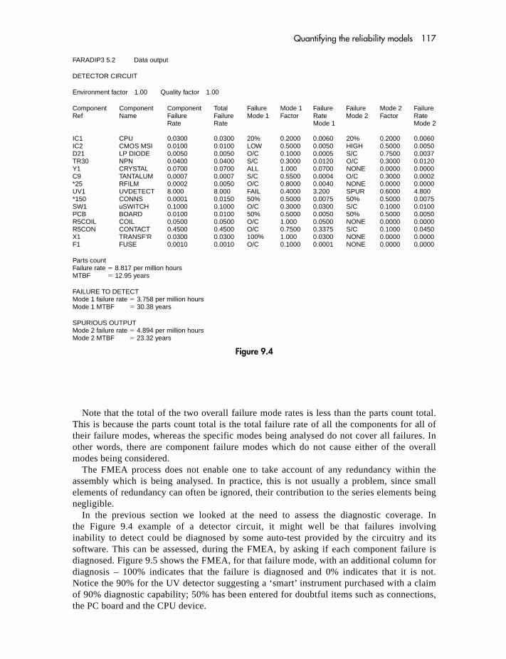
Quantifying the reliability models 117
Note that the total of the two overall failure mode rates is less than the parts count total.This is because the parts count total is the total failure rate of all the components for all oftheir failure modes, whereas the specific modes being analysed do not cover all failures. Inother words, there are component failure modes which do not cause either of the overallmodes being considered.
The FMEA process does not enable one to take account of any redundancy within theassembly which is being analysed. In practice, this is not usually a problem, since smallelements of redundancy can often be ignored, their contribution to the series elements beingnegligible.
In the previous section we looked at the need to assess the diagnostic coverage. Inthe Figure 9.4 example of a detector circuit, it might well be that failures involvinginability to detect could be diagnosed by some auto-test provided by the circuitry and itssoftware. This can be assessed, during the FMEA, by asking if each component failure isdiagnosed. Figure 9.5 shows the FMEA, for that failure mode, with an additional column fordiagnosis – 100% indicates that the failure is diagnosed and 0% indicates that it is not.Notice the 90% for the UV detector suggesting a ‘smart’ instrument purchased with a claimof 90% diagnostic capability; 50% has been entered for doubtful items such as connections,the PC board and the CPU device.
FARADIP3 5.2 Data output
DETECTOR CIRCUIT
Environment factor 1.00 Quality factor 1.00
Component Component Component Total Failure Mode 1 Failure Failure Mode 2 FailureRef Name Failure Failure Mode 1 Factor Rate Mode 2 Factor Rate
Rate Rate Mode 1 Mode 2
IC1 CPU 0.0300 0.0300 20% 0.2000 0.0060 20% 0.2000 0.0060IC2 CMOS MSI 0.0100 0.0100 LOW 0.5000 0.0050 HIGH 0.5000 0.0050D21 LP DIODE 0.0050 0.0050 O/C 0.1000 0.0005 S/C 0.7500 0.0037TR30 NPN 0.0400 0.0400 S/C 0.3000 0.0120 O/C 0.3000 0.0120Y1 CRYSTAL 0.0700 0.0700 ALL 1.000 0.0700 NONE 0.0000 0.0000C9 TANTALUM 0.0007 0.0007 S/C 0.5500 0.0004 O/C 0.3000 0.0002*25 RFILM 0.0002 0.0050 O/C 0.8000 0.0040 NONE 0.0000 0.0000UV1 UVDETECT 8.000 8.000 FAIL 0.4000 3.200 SPUR 0.6000 4.800*150 CONNS 0.0001 0.0150 50% 0.5000 0.0075 50% 0.5000 0.0075SW1 uSWITCH 0.1000 0.1000 O/C 0.3000 0.0300 S/C 0.1000 0.0100PCB BOARD 0.0100 0.0100 50% 0.5000 0.0050 50% 0.5000 0.0050R5COIL COIL 0.0500 0.0500 O/C 1.000 0.0500 NONE 0.0000 0.0000R5CON CONTACT 0.4500 0.4500 O/C 0.7500 0.3375 S/C 0.1000 0.0450X1 TRANSF’R 0.0300 0.0300 100% 1.000 0.0300 NONE 0.0000 0.0000F1 FUSE 0.0010 0.0010 O/C 0.1000 0.0001 NONE 0.0000 0.0000
Parts countFailure rate � 8.817 per million hoursMTBF � 12.95 years
FAILURE TO DETECTMode 1 failure rate � 3.758 per million hoursMode 1 MTBF � 30.38 years
SPURIOUS OUTPUTMode 2 failure rate � 4.894 per million hoursMode 2 MTBF � 23.32 years
Figure 9.4

118 Reliability, Maintainability and Risk
9.4 HUMAN FACTORS
9.4.1 Background
It can be argued that the majority of well-known major incidents, such as Three Mile Island,Bhopal, Chernobyl, Zeebrugge and Clapham, are related to the interaction of complex systemswith human beings. In short, the implication is that human error was involved, to a larger orgreater extent, in these and similar incidents. For some years there has been an interest inmodelling these factors so that quantified reliability and risk assessments can take account ofthe contribution of human error to the system failure.
As with other forms of reliability and risk assessment, the first requirement is for failure rate/probability data to use in the fault tree or whichever other model is used. Thus, human errorrates for various forms of activity are needed. In the early 1960s there were attempts to developa database of human error rates and these led to models of human error whereby rates could beestimated by assessing relevant factors such as stress, training, complexity and the like. Thesehuman error probabilities include not only simple failure to carry out a given task but diagnostictasks where errors in reasoning, as well as action, are involved. There is not a great deal of dataavailable (see Section 9.4.6) since:
� Low probabilities require large amounts of experience in order for a meaningful statistic toemerge.
� Data collection concentrates on recording the event rather than analysing the causes.� Many large organizations have not been prepared to commit the necessary resources to collect
data.
FARADIP3 5.2 Data output
DETECTOR CIRCUIT
FAILURE TO DETECT
Environment factor 1.00 Quality factor 1.00
Component Component Component Total Failure Mode 1 Failure DiagnosticRef Name Failure Failure Mode 1 Factor Rate Coverage
Rate Rate Mode 1 Mode 1
IC1 CPU 0.0300 0.0300 20% 0.2000 0.0060 50.00IC2 CMOS MSI 0.0100 0.0100 LOW 0.5000 0.0050 100.0D21 LP DIODE 0.0050 0.0050 O/C 0.1000 0.0005 0.0000TR30 NPN 0.0400 0.0400 S/C 0.3000 0.0120 100.0Y1 CRYSTAL 0.0700 0.0700 ALL 1.000 0.0700 100.0C9 TANTALUM 0.0007 0.0007 S/C 0.5500 0.0004 0.0000*25 RFILM 0.0002 0.0050 O/C 0.8000 0.0040 100.0UV1 UVDETECT 8.000 8.000 FAIL 0.4000 3.200 90.00*150 CONNS 0.0001 0.0150 50% 0.5000 0.0075 50.00SW1 uSWITCH 0.1000 0.1000 O/C 0.3000 0.0300 100.0PCB BOARD 0.0100 0.0100 50% 0.5000 0.0050 50.00R5COIL COIL 0.0500 0.0500 O/C 1.000 0.0500 100.0R5CON CONTACT 0.4500 0.4500 O/C 0.7500 0.3375 100.0X1 TRANSF’R 0.0300 0.0300 100% 1.000 0.0300 100.0F1 FUSE 0.0010 0.0010 O/C 0.1000 0.0001 100.0
Parts countFailure rate � 8.817 per million hoursMTBF � 12.95 years
FAILURE TO DETECTMode 1 failure rate � 3.758 per million hoursMode 1 MTBF � 30.38 yearsMode 1 diagnostic cover � 91.22%Mode 1 safe failure fraction � 96.26%
Figure 9.5

Quantifying the reliability models 119
More recently interest has developed in exploring the underlying reasons, as well as probabili-ties, of human error. In this way, assessments can involve not only quantification of the hazardousevent but also an assessment of the changes needed to bring about a reduction in error.
9.4.2 Models
There are currently several models, each developed by separate groups of analysts working in thisfield. Whenever several models are available for quantifying an event, the need arises to comparethem and to decide which is the most suitable for the task in hand. Factors for comparison could be:
� Accuracy – There are difficulties in the lack of suitable data for comparison and validation.� Consistency – Between different analysts studying the same scenario.� Usefulness – In identifying factors to change in order to reduce the human error rate.� Resources – Needed to implement the study.
One such comparison was conducted by a subgroup of the Human Factors in ReliabilityGroup, and their report Human Reliability Assessor’s Guide (SRDA R11), which addresseseight of the better-known models, is available from SRD, AEA Technology, Thomson House,Risley, Cheshire, UK WA3 6AT. The report is dated June 1995.
The following description of three of the available models will provide some understanding ofthe approach. A full application of each technique, however, would require a more detailed study.
9.4.3 HEART (Human Error Assessment and Reduction Technique)
This is a deterministic and fairly straightforward method developed by J. C. Williams during theearly 1980s. It involves choosing a human error probability from a table of error rates and thenmodifying it by multiplication factors identified from a table of error-producing conditions. It isconsidered to be of particular use during design since it identifies error-producing conditions andtherefore encourages improvements. It is a quick and flexible technique requiring few resources.The error rate table, similar to that given in Appendix 6, contains nine basic error task types. It is:
Task Probability of error
Totally unfamiliar, perform at speed, no idea of outcome 0.55
Restore system to new or original state on a single attempt without supervision or procedures checks 0.26
Complex task requiring high level of comprehension and skill 0.16
Fairly simple task performed rapidly or given scant attention 0.09
Routine highly practised, rapid task involving relatively lowlevel of skill 0.02
Restore system to new state following procedure checks 0.003
Totally familiar task, performed several times per hour, well motivated, highly trained staff, time to correct errors 0.0004
Respond correctly when there is augmented supervisory system providing interpretation 0.00002
Miscellaneous task – no description available 0.03

120 Reliability, Maintainability and Risk
The procedure then describes 38 ‘error-producing conditions’ to each of which a maximum mul-tiplier is ascribed. Any number of these can be chosen and, in turn, multiplied by a number between0 and 1 in order to take account of the analyst’s assessment of what proportion of the maximum touse. The modified multipliers are then used to modify the above probability. Examples are:
Error-producing condition Maximum multiplier
Unfamiliar with infrequent and important situation �17Shortage of time for error detection �11No obvious means of reversing an unintended action �8Need to learn an opposing philosophy �6Mismatch between real and perceived task �4Newly qualified operator �3Little or no independent checks �3Incentive to use more dangerous procedures �2Unreliable instrumentation �1.6Emotional stress �1.3Low morale �1.2Inconsistent displays and procedures �1.2Disruption of sleep cycles �1.1
The following example illustrates the way the tables are used to calculate a human error probability.Assume that an inexperienced operator is required to restore a plant bypass, using strict
procedures but which are different to his normal practice. Assume that he is not well aware ofthe hazards, late in the shift and that there is an atmosphere of unease due to worries aboutimpending plant closure.
The probability of error, chosen from the first table, might appropriately be 0.003.Five error-producing conditions might be chosen from the second table as can be seen in the
following table.For each condition the analyst assigns a ‘proportion of the effect’ from judgement (in the
range 0–1).The table is then drawn up using the calculation:
[(EPC � 1) � (Proportion)] � 1
The final human error probability is the multiple of the calculated values in the table timesthe original 0.003
Factor EPC Proportion [(EPC � 1) � (Proportion)] � 1effect
Inexperience 3 0.4 [(3 � 1) � (0.4)] � 1 � 1.8Opposite technique 6 1 6Low awareness of risk 4 0.8 3.4Conflicting objectives 2.5 0.8 2.2Low morale 1.2 0.6 1.12
Hence ERROR RATE 0.003 � 1.8 � 6 � 3.4 � 2.2 � 1.12 � 0.27

Quantifying the reliability models 121
Similar calculations can be performed at percentile bounds. The full table provides 5th and95th percentile bands for the error rate table.
Note that since the probability of failure cannot exceed one and, therefore, for calculationstaking the prediction above one it will be assumed that the error WILL almost certainly occur.
9.4.4 THERP (Technique for Human Error Rate Prediction)
This was developed by A. D. Swain and H. E. Guttmann and is widely used. The full procedurecovers the definition of system failures of interest, through error rate estimation, to recommend-ing changes to improve the system. The analyst needs to break each task into steps and thenidentify each error that can occur. Errors are divisible into types as follows:
Omission of a step or an entire taskSelects a wrong command or controlIncorrectly positions a controlWrong sequence of actionsIncorrect timing (early/late)Incorrect quantity
The sequence of steps is represented in a tree so that error probabilities can be multiplied alongthe paths for a particular outcome.
Once again (as with HEART), there is a table of error probabilities from which basic errorrates for tasks are obtained. These are then modified by ‘shaping parameters’ which takeaccount of stress, experience and other factors known to affect the error rates.
The analysis takes account of dependence of a step upon other steps. In other words, the failureof a particular action (step) may alter the error probability of a succeeding step.
9.4.5 TESEO (Empirical Technique To Estimate Operator Errors)
This was developed by G. C. Bellow and V. Colombari from an analysis of available literaturesources in 1980. It is applied to the plant control operator situation and involves an easilyapplied model whereby live factors are identified for each task and the error probability isobtained by multiplying together the five factors as follows:
Activity– Simple 0.001
Requires attention 0.01Non-routine 0.1
Time stress (in seconds available)– 2 (routine), 3 (non-routine) 10
10 (routine), 30 (non-routine) 120 (routine) 0.545 (non-routine) 0.360 (non-routine) 0.1
Operator– Expert 0.5
Average 1Poorly trained 3

122 Reliability, Maintainability and Risk
Anxiety– Emergency 3
Potential emergency 2Normal 1
Ergonomic (i.e. Plant interface)– Excellent 0.7
Good 1Average 3–7Very poor 10
Other methodsThere are many other methods such as:
SLIM (Success Likelihood Index Method)APJ (Absolute Probability Judgement)Paired ComparisonsIDA (The Influence Diagram Approach)HCR (Human Cognitive Reliability Correlation)
These are well described in the Human Factors in Reliability Group (HFRG) document mentionedabove.
9.4.6 Human error rates
Frequently there are not sufficient resources to use the modelling approach described above. Inthose cases a simple error rate per task is needed. Appendix 6 is a table of such error rateswhich has been put together as a result of comparing a number of published tables.
One approach, when using such error rates in a fault tree or other quantified method, is toselect a pessimistic value (the circumstances might suggest 0.01) for the task error rate. If, inthe overall incident probability computed by the fault tree, the contribution from that humanevent is negligible then the problem can be considered unimportant. If, however, the event dom-inates the overall system failure rate then it would be wise to rerun the fault tree (or simulation)using an error rate an order less pessimistic (e.g. 0.001). If the event still dominates the analysisthen there is a clear need for remedial action by means of an operational or design change. Ifthe event no longer dominates at the lower level of error probability then there is a grey areawhich will require judgement to be applied according to the circumstances. In any case, a moredetailed analysis is suggested.
A factor which should be kept in mind when choosing error rates is that human errors arenot independent. Error rates are likely to increase as a result of previous errors. For instance,an audible alarm is more likely to be ignored if a previous warning gauge has been recentlymisread.
In the 1980s it was recognized that a human error database would be desirable. In the USAthe NUCLARR database (see also Section 4.2.2.5) was developed and this consists of about50% human error data although this is heavily dependent on expert judgement rather thansolid empirical data. In the UK, there is the CORE-DATA (Computerized OperatorReliability and Error Database) which is currently being developed at the University ofBirmingham.

Quantifying the reliability models 123
9.4.7 Trends
Traditionally, the tendency has been to add additional levels of protection rather than addressthe underlying causes of error. More recently there is a focus of interest in analysing the under-lying causes of human error and seeking appropriate procedures and defences to minimize oreliminate them.
Regulatory bodies, such as the UK Health and Safety Executive, are taking a greater interestin this area and questions are frequently asked about the role of human error in the hazardassessments which are a necessary part of the submissions required from operators of majorinstallations (see Chapter 21).
Figure 9.6 is an example of applying HEART and TESEO to a specific task. The questionshave been abbreviated onto a spread sheet which calculates the predictions.
9.5 SIMULATION
9.5.1 The technique
Block Diagram, Fault Tree and Cause Consequence analyses were treated, in Chapters 7–9, asdeterministic methods. In other words, given that the model is correct then for given data thereis only one answer to a model. If two components are in series reliability (fault tree OR gate)then, if each has a failure rate of 5 per million hours, the overall failure rate is 10 per millionhours – no more, no less. Another approach is to perform a computer-based simulation, some-times known as Monte Carlo analysis, in which random numbers are used to sample from prob-ability distributions.
In the above example, two random distributions each with a rate of 5 per million would beset up. Successive time slots would be modelled by sampling from the two distributions inorder to ascertain if either distribution yielded a failure in that interval.
One approach, known as event-driven simulation inverts the distribution to representtime as a function of the probability of a failure occurring. The random number generatoris used to provide a probability of failure which is used to calculate the time to the nextfailure. The events generated in this manner are then logged in a ‘diary’ and the systemfailure distribution derived from the component failure ‘diary’. As an example assume wewish to simulate a simple exponential distribution then the probability of failing in time t isgiven by:
R(t) � e��t
Inverting the expression we can say that:
t � (loge R)/�
Since R is a number between 0 and 1 the random number generator can be used to providethis value which is divided by � to provide the next value of t. The same approach is adoptedfor more complex expressions such as the Weibull.
A simulation would be run many thousands of times and the overall rate of system failurecounted. This might be 10 per million of 9.99998 or 10.0012 and, in any case, will yieldslightly different results for each trial. The longer each simulation run and the more runsattempted, the closer will the ultimate answer approximate to 10 per million.
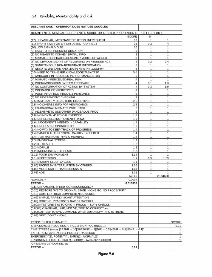
124 Reliability, Maintainability and Risk
DESCRIBE TASK – OPERATOR DOES NOT USE GOGGLES
HEART: ENTER NOMINAL ERROR. ENTER SCORE OR 1. ENTER PROPORTION [0 � 1] EFFECT OR 1.SCORE %
(17) UNFAMILIAR, IMPORTANT SITUATION, INFREQUENT 17 1 1(11) SHORT TIME FOR ERROR DETECT/CORRECT 11 0.3 4(10) LOW SIGNAL/NOISE 10 1 1(9) EASY TO SUPPRESS INFORMATION 9 1 1(8) NO MEANS TO CONVEY SPATIAL INFO 8 1 1(8) MISMATCH OPERATOR/DESIGNER MODEL OF WORLD 8 1 1(8) NO OBVIOUS MEANS OF REVERSING UNINTENDED ACT 8 0.2 2.4(6) SIMULTANEOUS NON-REDUNDANT INFORMATION 6 1 1(6) NEED TO UNLEARN AND LEARN NEW PHILOSOPHY 6 1 1(5.5) NEED TO TRANSFER KNOWLEDGE TASK/TASK 5.5 1 1(5) AMBIGUITY IN REQUIRED PERFORMANCE STD’s 5 1 1(4) MISMATCH PERCEIVED/REAL RISK 4 1 1(4) POOR/AMBIGUOUS SYSTEM FEEDBACK 4 0.1 1.3(4) NO CONFORMATION OF ACTION BY SYSTEM 4 0.3 1.9(3) OPERATOR INEXPERIENCED 3 1 1(3) POOR INFO FROM PROC’S & PERSONS’s 3 1 1(3) NO INDEPENDENT CHECKING 3 1 1(2.5) IMMEDIATE V LONG-TERM OBJECTIVES 2.5 1 1(2.5) NO DIVERSE INFO FOR VERIFICATION 2.5 1 1(2) EDUCATIONAL MISMATCH WITH TASK 2 1 1(2) INCENTIVE TO USE OTHER DANGEROUS PROC 2 1 1(1.8) NO MENTAL/PHYSICAL EXERCISE 1.8 1 1(1.6) UNRELIABLE INSTRUMENTs (known) 1.6 1 1(1.6) JUDGEMENTS NEEDED � CAPABILITY 1.6 1 1(1.6) UNCLEAR RESPONSIBILITY 1.6 1 1(1.4) NO WAY TO KEEP TRACK OF PROGRESS 1.4 1 1(1.4) DANGER THAT PHYSICAL CAPAB’s EXCEEDED 1.4 1 1(1.4) TASK HAS NO INTRINSIC MEANING 1.4 1 1(1.3) EMOTIONAL STRESS 1.3 1 1(1.2) ILL HEALTH 1.2 1 1(1.2) MORALE 1.2 1 1(1.2) INCONSISTENT DISPLAYS 1.2 1 1(1.15) POOR ENVIRONMENT 1.15 1 1(1.1) REPETITIOUS 1.1 0.9 1.09(1.1) DISRUPT SLEEP CYCLES 1.1 1 1(1.06) PACING BY INTERRUPTION BY OTHERS 1.06 1 1(1.03) MORE STAFF THAN NECESSARY 1.03 1 1(1.02) AGE 1.02 1 1
145.66 25.84608NOMINAL � 0.0004ERROR � 0.010338(0.5) UNFAMILIAR, SPEED, CONSEQUENCES??(0.26) RESTORE SYS TO ORIGINAL STATE IN ONE GO. NO PROCS/SUPY(0.16) COMPLEX, HIGH COMPREHENSION/SKILL(0.09) SIMPLE, RAPIDLY, SCANT ATTENTION(0.02) ROUTINE, PRACTISED, RAPID LOW SKILL(0.003) RESTORE SYS TO ORIG � PROCS � SUPY CHECKS(0.0004) V FAMILIAR, n/HR, MOTIVE, TIME TO CORRECT, etc(0.00002) RESP TO SYS COMMAND WHEN AUTO SUPY INFO IS THERE(0.03) MISC (DON’T KNOW)
TESEO: ENTER ESTIMATES SCORESIMPLE(0.001), REQUIRES ATT(0.01), NON-ROUTINE(0.1) 0.01TIME STRESS (secs), [2R3NR � 10][10R30NR � 1][20R � 0.5][45NR � 0.3][60NR � 0.1]* 1EXPERT(0.5), AVERAGE(1), POORLY TRAINED(3) 1EMERGENCY(3), POTENTIAL EMRG(2), NORMAL(1) 1ERGONOMIC EXCELLENT(0.7), GOOD(1), AV(3–7)VPOOR(10) 1*2R MEANS 2s ROUTINE, etc.ERROR � 0.01
Figure 9.6
Quantifying the reliability models 125
This may seem a laborious method for assessing what can be obtained more easily from deter-ministic methods. Fault Tree, Cause Consequence and Simple Block diagram methods are,however, usually limited to simple AND/OR logic and constant failure rates and straightforwardmean down times.
Frequently problems arise due to complicated failure and repair scenarios where the effect offailure and the redundancy depend upon demand profiles and the number of repair teams. Also,it may be required to take account of failure rates and down times which are not constant. Theassessment may therefore involve:
� Log Normal down times� Weibull down times� Weibull (not constant) failure rates� Standby items with probabilities of successful start� Items with variable profiles for which the MTBF varies with some process throughput� Spares requirements� Maintenance skill types and quantities� Logistical delays� Ability to make-up lost availability within defined rules and limits
It is not easy to evaluate these using the techniques already explained in this chapter and, forthem, simulation now provides a quick and cost-effective method.
One drawback to the technique is that the lower the probability of the events, the greaterthe number of trials that are necessary in order to obtain a satisfactory result. The other,which has recently become much reduced, was the program cost and computer run timesinvolved, which were greatly in excess of fault tree and block diagram approaches. Withever-increasing PC power there are now a number of cost-effective packages which can rivalthe deterministic techniques.
A recent development in reliability simulation (see Section 9.5.2) is the use of genetic algo-rithms. This technique enables modelling options (e.g. additional redundant streams) to bespecified in the simulation. The algorithm then develops and tests the combinations of possibili-ties depending on the relative success of the outcomes.
There are a variety of algorithms for carrying out this approach and they are used in thevarious PC packages which are available. Some specific packages are described in thefollowing sections. There are many similarities between them.
9.5.2 Some packages
9.5.2.1 OPTAGONThis package was developed by Advantica (formerly British Gas Research and Development) tolink availability, reliability, operational and commercial information together in order to allowoverall performance to be optimized. It is a development of the earlier packages SWIFT andPARAGON and is primarily intended for modelling the performance of oil and gas productionassets where there are complexities that require a high level of functionality. These complexitiesinclude:
� Multiple revenue streams and product streams.� Tank storage and shipping (e.g. LNG import and export facilities).� Gas substitution arrangements.

126 Reliability, Maintainability and Risk
� Operational strategy (e.g. over-producing to make-up for production losses).� Resource constraints (e.g. repair team limitations, spares holding).� Variable demand profile (e.g. seasonal) with random fluctuations.� Partial states of operation.� System configuration changes and equipment throughput variations.� Well profiles.� Conditional logic and equipment dependencies.
The package uses the Monte Carlo approach to overcome the modelling complexities. Thisapproach consists of explicitly modelling the system being studied, subjecting it to a typical set ofevents over its lifetime, and empirically observing how well it performs. The typical events thatare directed at the model are generated stochastically and this means that any individualsimulation of the system’s lifetime cannot be taken as a guide to its average performance – themodel may have been subject to events that were more or less favourable than the average.Instead, it is necessary to carry out a large number of individual simulations. The performance ofthe model over many simulations gives an indication of how it is likely to perform on average, andhow widely the range of possible performance is spread. The application of this approach inOPTAGON enables not only the prediction of mean values for availability statistics such asproduction availability, shortfall, operational availability, etc., but also enables the possible rangeof likely performance to be estimated using P5, P10, P50 (median), P90, P95. For example, theP10 value for shortfall is the value for which there is a 10% probability that the shortfall will beless than this value and a 90% probability that the shortfall will be greater. This can give moreuseful information than purely quoting mean values as it provides an indication of the likely rangeof performance.
A particular feature is the use of the Genetic Algorithms already mentioned. These apply theDarwinian principle of natural selection by searching for the optimal solution emerging fromthe successive simulation runs. It is achieved by expressing the characteristics of a system(such as the complexities listed earlier) in the form of a binary string. The string (known as agene-string) can then be created by random number generation. A weighting process is used tofavour those genes which lead to the more optimistic outcomes by increasing the probabilityof their choice in successive simulations.
The OPTAGON tool was first developed in 1990 by Advantica. Since then it has beenused on a large number of applications representing interests in the UK and worldwide.
9.5.2.2 MAROS, TAROO, TRAIL and ACEThese packages are from Jardine Technology who have progressed the development and useof simulation software for RAM and asset performance analyses over the last 20 years. Theoriginal platform has now been developed into a range of simulators targeted at specificmarkets and end-users. All the simulators in Jardine’s portfolio utilize the same core methodof statistical sampling (Discrete Event Simulation) to determine at what point in time thenext event will occur, and then move directly in simulation time from one event to the next.At each event, the simulator applies an extensive rule set to determine what the impact tothe asset will be. The simulator must then take a decision based upon maintenance logisticsin order to progress to the next event. After resolving the rule sets and processing events,any resultant impact on asset performance is recorded. This direct simulation approachallows much more complex systems, logistics and interactions to be analysed than could beapproached via any implementation of static calculation. All the simulators have a graphicalinterface that enables extremely rapid and user friendly means of simulation model building.There are four simulation packages MAROS, TARO, TRAIL and ACE.

Quantifying the reliability models 127
1. MAROS – tailored for use in the oil and gas industry with extensive features for modellingoffshore installations and onshore plants, production networks, shipping, incorporatingmaintenance, logistics, production operations and customer demand scenarios.
2. TARO – developed for the downstream petrochemical and refining industry to capturethe complex interaction of: unit and equipment reliability; multiple feed, intermediateand product streams; storage tanks; and operational strategies (including shipping, railcarand pipeline distribution).
3. TRAIL – developed for the railway industry; has been used extensively on the UK’s networkupgrade projects. TRAIL is able to assess the impact from infrastructure failures (e.g. signals,p-way, and points) and operation perturbations (e.g. weather, crew availability) on a runningtimetable in terms of delays accrued per journey and overall service punctuality. TRAILprovides a quantitative basis for evaluating design, maintenance, and operational changes tothe railways with a view to optimising service delivery performance.
4. ACE is a cut down version of MAROS that removes the functionality specific to the oiland gas industries. It is therefore a general purpose discrete event simulation package forreliability/availability analyses. ACE features a ‘wizard’ type interface that guides the userthrough the construction of a RAM model and enables reliability data to be selected froman integral library.
They are available from Jardine Technology Ltd, Glasgow, UK www.jardinesolutions.com
9.5.2.3 RAM4, RAMP and SAMThese packages are from Advantage Technical Consulting www.advantage-business.co.uk
RAM4RAM4 is a Reliability Block Diagram (RBD) tool, has been developed for modelling continuouslyrunning systems, and is mission oriented. Typical applications include communications, defence,control systems, signalling and space systems. RAM4 is sponsored by the Ministry of Defence,and is a recommended modelling tool for MoD projects.
RAM4 gives design and reliability engineers a powerful, easy to use analysis tool for theassessment of the reliability of complex repairable and non-repairable systems – whetherelectronic, mechanical or a mixture of both – as described by RBDs. The program has beencontinually enhanced and currently includes features such as:
� Finite spares and maintenance resources.� Preventive maintenance schedules.� Logistic delays.� Startup delays for standby items.� Equipment wear out (Weibull failure distribution).� Common mode failures.� Active and standby redundancy.� Queuing for repairs.� Simulation lifetime.(www.advantage-business.co.uk)
RAMPRAMP is a powerful availability modelling tool for the analysis of process systems. RAMP issimilar to RAM4 in that it is a RBD based tool. However, as well as modelling system availability,RAMP models may be created to investigate the effects of scheduled and unscheduled downtime

128 Reliability, Maintainability and Risk
on process throughput, establishing relationships between equipment reliability, configuration,maintenance strategy, spares and resources. RAMP built-in features are similar to those of RAM4but additionally include:
� Time varying delivery and demand/nomination profiles.� Bulk and buffer stores.
SAMThe Systems Availability Model (SAM) is a program designed to assess the RAM characteristics ofmultiple systems used over operating scenarios that place varying demands upon those systems,such as that encountered in complex military or industrial installations. It is the ability of SAM tooverlay system dependencies onto complex mission profiles that makes it a powerful and flexibleRAM modelling tool. A mission profile may be built up of a variety of activities each demandinguse of different combinations of equipments, rather than a fixed time at risk approach adopted bymany simpler modelling tools.
9.5.2.4 ITEM ToolkitThis is also a Monte Carlo package based on reliability block diagrams. It copes with revealedand unrevealed failures, preventive and corrective maintenance regimes, ageing and mainte-nance queuing. The usual standby and start-up scenarios are modelled and non-random distri-butions for failure rate and down time can be modelled. System performance is simulated over anumber of life-cycles to predict unavailability, number of system failures and required spareslevels. ITEM are at Fareham, Hants (www.itemuk.com).
9.6 COMPARING PREDICTIONS WITH TARGETS
In the light of the work described in Section 4.4 we saw that is now possible to attempt somecorrelation between predicted and field reliability and that the confidence in the predictiondepends upon the data used.
The studies referred to indicated that the results were equally likely to be optimistic as pes-simistic. Therefore one interpretation is that we are 50% confident that the field result will beequal to or better than the predicted RAMS value. However, a higher degree of confidence maybe desired, particularly if the RAMS prediction is for a safety-related failure mode. If industryspecific data has been used for the prediction and 90% confidence is required then, consultingthe tables in Section 4.4, a failure rate of 4 times the predicted value would be used.
If the ‘4 times failure rate’ figure is higher than the value which coincides with the MaximumTolerable Risk, discussed in Sections 3.2 and 10.2, then the proposed design is not acceptable.If it falls between the Maximum Tolerable and Broadly Acceptable Risk values then theALARP principle is applied as shown in the cost per life saved examples in Section 3.3.
The following is an example:The maximum tolerable risk of fatality associated with a particular system failure mode
might be 10�4 per annum. The failure rate, for that mode, which risk assessment shows isassociated with that frequency, is say 10�3 failures per annum. If the broadly acceptable riskis 10�6 per annum then it follows that it will be achieved with a failure rate 100 times less,10�4 per annum.
Let the predicted failure rate (using industry specific data) for the system failure mode inquestion be 2 � 10�4 per annum and assume that we wish to be 90% confident in the result. Asdiscussed above the 90% confidence failure rate would be 4 � 2 � 10�4 � 8 � 10�4 per annum.

Quantifying the reliability models 129
In other words we can be 90% sure that the field failure rate will be better than 8 � 10�4 perannum (in other words a fatality risk of 8 � 10�5 per annum).
This is better than the maximum tolerable risk but not small enough to be ‘dismissed’ asbroadly acceptable. Therefore, a design proposal is made (perhaps additional redundancy at acost of £5000) to improve the failure rate. Assume that the outcome is a new predicted failurerate of 10�4 per annum (i.e. 4 � 10�4 at 90% confidence which is 4 � 10�5 per annum riskof fatality).
Assuming 2 fatalities and a 40 year system life, the cost per life saved calculation is:
£5000/([8 � 10�5 � 4 � 10�5] 2 � 40) � £1.5 million
If this exceeds the cost per life saved criteria being applied (see Section 3.3.2) then the existingdesign would be considered to offer an integrity which is ALARP. If not then the design proposalwould need to be considered.
The same technique may be applied to production loss as well as to safety. TheUnavailability of a process can be predicted and used to assess the cost of outage that can beanticipated. Thus, a process for which outage costs £50 000 per day, and having a predictedunavailability of 5 � 10�3 will lose:
£50 000 � 5 � 10�3 � 365 � £91 250 per annum.
Suppose that a proposed modification, involving redundant items, is assessed to cost £100 000and that it improves the unavailability from 5 � 10�3 to 8 � 10�4.
The saving is thus:
£50 000 � (5 � 10�3 � 8 � 10�4) � 365 � £76 650 per annum.
It would therefore seem that the proposed modification is acceptable.
EXERCISES
1. The reliability of the two-valve example of Figure 2.1 was calculated, for two failure modes,in Sections 7.3 and 7.4. Imagine that, to improve the security of supply, a twin parallelstream is added as follows:
Construct reliability block diagrams for:
(a) Loss of supply(b) Failure to control downstream over-pressure
and recalculate the reliabilities for one year.
2. For this twin-stream case, imagine that the system is inspected every two weeks, for valveswhich have failed shut. (a) How does this affect the system failure rate in respect of loss ofsupply? (b) Now calculate the effect of addressing CCF (say 5%).
3. In Section 8.3, the Cutsets were ranked by failure rate. Repeat this ranking by unavailability.

10 Risk assessment (QRA)
10.1 FREQUENCY AND CONSEQUENCE
Having identified a hazard, the term ‘risk analysis’ is often used to embrace two types ofassessment:
� The frequency (or probability) of the event� The consequences of the event
Thus, for a process plant the assessments could be:
� The probability of an accidental release of a given quantity of toxic (or flammable) materialmight be 1 in 10 000 years.
� The consequence, following a study of the toxic (or thermal radiation) effects and havingregard to the population density, might be 40 fatalities.
The term QRA (Quantified Risk Assessment) refers to the process of assessing the frequencyof an event and its measurable consequences (e.g. fatalities, damage).
The analysis of consequence is a specialist area within each industry and may be basedon chemical, electrical, gas or nuclear technology. Prediction of frequency is essentiallythe same activity as reliability prediction, the methods for which have been described inChapters 7–9. In many cases the method is identical, particularly where the event is dependentonly on:
� Random hardware (component) failures� Systematic failures� Human error� Software
Both aspects of quantitative risk assessment have received increasing attention over the years,particularly following Lord Cullen’s inquiry into the Piper Alpha disaster.
Risk analysis, also involves factors such as lightning, collision, weather factors, flood, etc.These are dealt with in Section 10.4.
10.2 PERCEPTION OF RISK AND ALARP
The question arises of quantifying the risk of fatality. The meaning of such words as ‘tolerable’,‘acceptable’ and ‘unacceptable’ becomes important. There is, of course, no such thing as zerorisk and it becomes necessary to think about what levels are ‘tolerable’ or even ‘acceptable’.
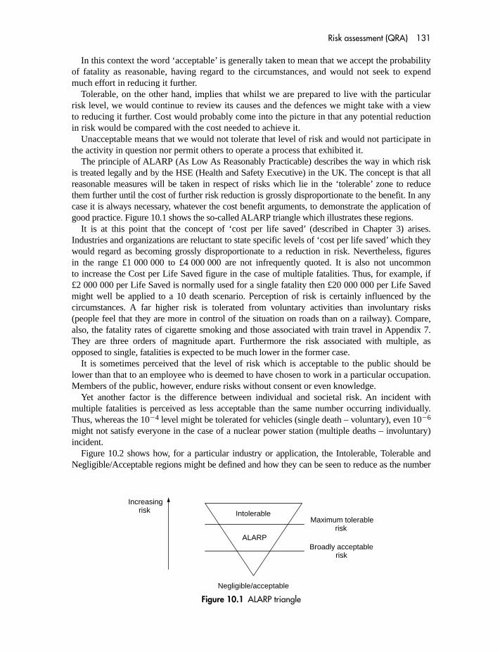
Risk assessment (QRA) 131
In this context the word ‘acceptable’ is generally taken to mean that we accept the probabilityof fatality as reasonable, having regard to the circumstances, and would not seek to expendmuch effort in reducing it further.
Tolerable, on the other hand, implies that whilst we are prepared to live with the particularrisk level, we would continue to review its causes and the defences we might take with a viewto reducing it further. Cost would probably come into the picture in that any potential reductionin risk would be compared with the cost needed to achieve it.
Unacceptable means that we would not tolerate that level of risk and would not participate inthe activity in question nor permit others to operate a process that exhibited it.
The principle of ALARP (As Low As Reasonably Practicable) describes the way in which riskis treated legally and by the HSE (Health and Safety Executive) in the UK. The concept is that allreasonable measures will be taken in respect of risks which lie in the ‘tolerable’ zone to reducethem further until the cost of further risk reduction is grossly disproportionate to the benefit. In anycase it is always necessary, whatever the cost benefit arguments, to demonstrate the application ofgood practice. Figure 10.1 shows the so-called ALARP triangle which illustrates these regions.
It is at this point that the concept of ‘cost per life saved’ (described in Chapter 3) arises.Industries and organizations are reluctant to state specific levels of ‘cost per life saved’ which theywould regard as becoming grossly disproportionate to a reduction in risk. Nevertheless, figuresin the range £1 000 000 to £4 000 000 are not infrequently quoted. It is also not uncommonto increase the Cost per Life Saved figure in the case of multiple fatalities. Thus, for example, if£2 000 000 per Life Saved is normally used for a single fatality then £20 000 000 per Life Savedmight well be applied to a 10 death scenario. Perception of risk is certainly influenced by thecircumstances. A far higher risk is tolerated from voluntary activities than involuntary risks(people feel that they are more in control of the situation on roads than on a railway). Compare,also, the fatality rates of cigarette smoking and those associated with train travel in Appendix 7.They are three orders of magnitude apart. Furthermore the risk associated with multiple, asopposed to single, fatalities is expected to be much lower in the former case.
It is sometimes perceived that the level of risk which is acceptable to the public should belower than that to an employee who is deemed to have chosen to work in a particular occupation.Members of the public, however, endure risks without consent or even knowledge.
Yet another factor is the difference between individual and societal risk. An incident withmultiple fatalities is perceived as less acceptable than the same number occurring individually.Thus, whereas the 10�4 level might be tolerated for vehicles (single death – voluntary), even 10�6
might not satisfy everyone in the case of a nuclear power station (multiple deaths – involuntary)incident.
Figure 10.2 shows how, for a particular industry or application, the Intolerable, Tolerable andNegligible/Acceptable regions might be defined and how they can be seen to reduce as the number
Increasingrisk Intolerable
Maximum tolerablerisk
ALARPBroadly acceptable
risk
Negligible/acceptable
Figure 10.1 ALARP triangle

132 Reliability, Maintainability and Risk
of fatalities increases. Thus for a single fatality (left hand axis) risks of 10�5 to 10�3 are regardedas ALARP. Above 10�3 is unacceptable and below 10�5 is acceptable. For 10 fatalities, however,the levels are 10 times more stringent. This topic is treated very fully in the HSE publication, TheTolerability of Risk from Nuclear Power Stations and its more recent publication Reducing RisksProtecting People.
10.3 HAZARD IDENTIFICATION
Before an event (failure) can be quantified it must first be identified and there are a numberof formal procedures for this process. Hazard Identification (HAZID) is used to identify thepossible hazards, HAZOP (Hazard and Operability Studies) is used to establish how thehazards might arise in a process whereas HAZAN (Hazard Analysis) refers to the process ofanalysing the outcome of a hazard. This is known as Consequence Analysis.
This is carried out at various levels of detail from the earliest stages of design throughout theproject design cycle.
Preliminary Hazard Analysis, at the early system design phase, identifies safety criticalareas, identifies and begins to quantify hazards and begins to set safety targets. It mayinclude:
Previous experience (historical information)Review of hazardous materials, energy sources, etc.Interfaces with operators, public, etc.Applicable legislation, standards and regulationsHazards from the environmentImpact on the environmentSoftware implicationsSafety-related equipment
10–2
10–4
1 10 100
Number of fatalities
Fre
quen
cy o
f tha
t num
ber
of fa
talit
ies
1000
Intolerable region
Negligible/acceptable region
Tolerable (ALARP) range
10–3
10–5
10–6
10–7
Figure 10.2 (Example only)

Risk assessment (QRA) 133
More detailed Hazard Analysis follows in the detailed design stages. Now that specific hardwaredetails are known and drawings exist, studies can address the effects of failure at component andsoftware level. FMEA and Fault Tree techniques (Chapter 8) as well as HAZOP and ConsequenceAnalyses are applicable here.
10.3.1 HAZOP
HAZOP (Hazard and Operability Studies) is a technique, developed in the 1970s, by lossprevention engineers working for Imperial Chemical Industries at Tees-Side UK. The purposeof a HAZOP is to identify hazards in the process. At one time this was done by individuals orgroups of experts at a project meeting. This slightly blinkered approach tended to focus onthe more obvious hazards and those which related to the specific expertize of the participants.In contrast to this, HAZOP involves a deliberately chosen balanced team using a systematicapproach. The method is to systematically brainstorm the plant, part by part, and to reviewhow deviations from the normal design quantities and performance parameters would affectthe situation. Appropriate remedial action is then agreed.
One definition of HAZOP has been given as:
A Study carried out by a Multidisciplinary Team, who apply Guidewords to identifyDeviations from the Design Intent of a system and its Procedures. The team attempt toidentify the Causes and Consequences of these Deviations and the Protective Systemsinstalled to minimize them and thus to make Recommendations which lead to Risk Reduction.
This requires a full description of the design (up-to-date engineering drawings, linediagrams, etc.) and a full working knowledge of the operating arrangements. A HAZOP isthus usually conducted by a team which includes designers and operators (including plant,process and instrumentation) as well as the safety (HAZOP) engineer.
A typical small process plant might be ‘HAZOPed’ by a team consisting of:
Chemical EngineerMechanical EngineerInstrument EngineerLoss Prevention (or Safety or Reliability) EngineerChemistProduction Engineer/ManagerProject Manager
A key feature is the HAZOP team leader who must have experience of HAZOP and be full timein the sense that he attends the whole study whereas some members may be part time. Anessential requirement for the leader is experience of HAZOP in other industries so as to bringas wide a possible view to the probing process. Detailed recording of problems and actions isessential – during the meeting. Follow-up and review of actions must also be formal. Theremust therefore be a full-time Team Secretary who records all findings and actions.
The procedure will involve:
Define the scope and objectives of the HAZOPDefine the documentation requiredSelect the teamPrepare for the HAZOP (pre-reading)

134 Reliability, Maintainability and Risk
Carry out and record the HAZOPImplement the follow-up actionRecord results
In order to formalize the analysis a ‘guideword’ methodology has evolved in order to point theanalysts at the types of deviation. The guidewords are applied to each of the process parameterssuch as flow, temperature, pressure, etc. under normal operational as well as start-up andshut-down modes. Account should be taken of safety systems which are allowed, under specifiedcircumstances, to be temporarily defeated. The following table describes the approach:
Guideword Meaning Explanation
NO or NOT The parameter is zero Something does not happenbut no other effect
MORE THAN or LESS THAN There are increases Flows and temperatures areor decreases in the not normalprocess parameter
AS WELL AS Qualitative Increase Some additional effect
PART OF Qualitative Increase Partial effect (not all)
THE REVERSE Opposite Reverse flow or material
OTHER THAN Substitution Totally different effect
Each deviation of a parameter must have a credible cause, typically a component or humanerror related failure or a deviation elsewhere in the plant. Examples of typical causes might be:
Deviation Cause
More Flow Line ruptureControl valve fail ‘open’
Less Flow Control valve fail ‘closed’Leaking vessel or heat exchanger
No Flow BlockageRupture
Reverse Flow SiphoningCheck-valve failure
More Pressure Restricted FlowBoiling
Less/No Pressure Excessive Flow outInsufficient Flow in
More Level Operator errorVessel leak
Less/No Level Drain left openHigh barometric pressure
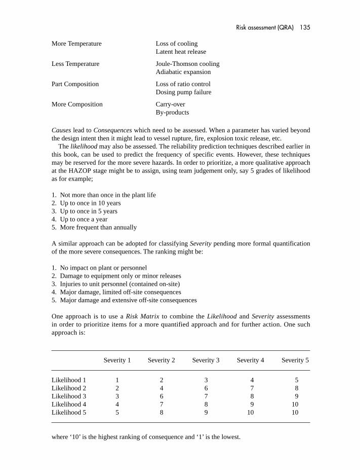
Risk assessment (QRA) 135
More Temperature Loss of coolingLatent heat release
Less Temperature Joule-Thomson coolingAdiabatic expansion
Part Composition Loss of ratio controlDosing pump failure
More Composition Carry-overBy-products
Causes lead to Consequences which need to be assessed. When a parameter has varied beyondthe design intent then it might lead to vessel rupture, fire, explosion toxic release, etc.
The likelihood may also be assessed. The reliability prediction techniques described earlier inthis book, can be used to predict the frequency of specific events. However, these techniquesmay be reserved for the more severe hazards. In order to prioritize, a more qualitative approachat the HAZOP stage might be to assign, using team judgement only, say 5 grades of likelihoodas for example;
1. Not more than once in the plant life2. Up to once in 10 years3. Up to once in 5 years4. Up to once a year5. More frequent than annually
A similar approach can be adopted for classifying Severity pending more formal quantificationof the more severe consequences. The ranking might be:
1. No impact on plant or personnel2. Damage to equipment only or minor releases3. Injuries to unit personnel (contained on-site)4. Major damage, limited off-site consequences5. Major damage and extensive off-site consequences
One approach is to use a Risk Matrix to combine the Likelihood and Severity assessmentsin order to prioritize items for a more quantified approach and for further action. One suchapproach is:
Severity 1 Severity 2 Severity 3 Severity 4 Severity 5
Likelihood 1 1 2 3 4 5Likelihood 2 2 4 6 7 8Likelihood 3 3 6 7 8 9Likelihood 4 4 7 8 9 10Likelihood 5 5 8 9 10 10
where ‘10’ is the highest ranking of consequence and ‘1’ is the lowest.

136 Reliability, Maintainability and Risk
HAZOP was originally applied to finalized plant design drawings. However, changes arising atthis stage can be costly and the technique has been modified for progressive stages of applicationthroughout the design cycle. As well as being a design tool HAZOP can be equally successfullyapplied to existing plant and can lead to worthwhile modifications to the maintenance procedures.
Typical phases of the life-cycle at which HAZOP might be applied are:
CONCEPTUAL DESIGNDETAILED DESIGNAPPROVED FOR CONSTRUCTION‘AS-BUILT’PROPOSED MODIFICATIONSREGULATORY REQUIREMENTS
HAZOP can be applied to a wide number of types of equipment including:
Process plantTransport systemsData and programmable systems (see UK DEF STD 0058)Buildings and structuresElectricity generation and distributionMechanical equipmentMilitary equipment
In summary, HAZOP study not only reveals potential hazards but leads to a far deeperunderstanding of a plant and its operations.
Appendix 11 provides a somewhat simple example of a HAZOP.
10.3.2 HAZID
Whereas HAZOP is an open-ended approach, HAZID is a checklist technique. At an earlystage, such as the feasibility study for a hazardous plant, HAZID enables the major hazards tobe identified. At the conceptual stage a more detailed HAZID would involve designing outsome of the major problems.
Often, the HAZID uses a questionnaire approach and each organization tends to develop andevolve its own list, based on experience. Appendix 12 gives an example of such a list and isreproduced by kind permission of the Institution of Gas Engineers (guidance document SR24).
10.3.3 HAZAN (Consequence Analysis)
This technique is applied to selected hazards following the HAZOP and HAZID activities.It is usually the high-consequence activities such as major spillage of flammable or toxicmaterials or explosion which are chosen. High-consequence scenarios usually tend to be thelow-probability hazards.
Consequence analysis requires a detailed knowledge of the materials/hazards involved inorder to predict the outcome of the various failures. The physics and chemistry of the outcomesis necessary in order to construct mathematical models necessary to calculate the effects onobjects and human beings. Some examples are:
Flammable and toxic releases (heat radiation, food/water pollution and poisoning)Structural collapse

Risk assessment (QRA) 137
Vehicle, ships and other impact (on structures and humans)Nuclear contaminationExplosion (pressure vessels and chemicals)Large scale water release (vessels, pipes and dams)
Reference to specific literature, in each case, is necessary.
10.4 FACTORS TO QUANTIFY
The main factors which may need to be quantified in order to assess the frequency of an eventare as follows.
10.4.1 Reliability
Chapters 7–9 cover this element in detail.
10.4.2 Lightning and thunderstorms
It is important to differentiate between thunderstorm-related damage, which affects electricalequipment by virtue of induction or earth currents, and actual lightning strikes. The former isapproximately one order (ten times) more frequent.
BS 6651: 1990 indicates an average of 10 thunderstorm days per annum in the UK. Thisvaries, according to the geography and geology of the area, between 3 and 21 days per annum.Thunderstorm damage (usually electrical) will thus be related to this statistic. Some informaldata suggest damage figures such as:
� Five incidents per square kilometre per annum where electrical equipment is used in outdooror unprotected accommodation.
� 0.02 incidents per microwave tower.
Lightning strike, however, is a smaller probability and the rate per annum is derived bymultiplying the effective area in square kilometres by the strikes per annum per squarekilometre in Figure 10.3 (reproduced by kind permission of the British Standards Institution).The average is in the area of 0.3–0.5 per annum.
The effective area is obtained by subtending an angle of 45° around the building or objectin question. Figure 10.4 illustrates the effect upon one elevation of a square building of side10 m and height 2 m. The effective length is thus 14 m (10 � 2 � 2). BS 6651: 1990, fromwhich Figure 10.3 is reproduced, contains a fuller method of assessment.
It must not be inferred, automatically, that a strike implies damage. This will depend uponthe substance being struck, the degree of lightning protection and the nature of the equipmentcontained therein.
10.4.3 Aircraft impact
Aircraft crash is a high-consequence but a low-probability event. The data are well recorded anda methodology has evolved for calculating the probability of impact from a crashing aircraftaccording to the location. This type of study stemmed from concerns when carrying out risk

138 Reliability, Maintainability and Risk
Figure 10.3 Number of lightning flashes to the ground per km2 per year for the UK
Figure 10.4

Risk assessment (QRA) 139
assessments of a nuclear plant but can be used for any other safety study where impact damageis relevant.
This subject is extensively covered in The calculation of aircraft risk in the UK, J. P. Byrne,AEA Technology, Report 150, 1997 (HSE Books ISBN 0 7176 1447 6).
Crashes are considered as if from two (additive) causes and approximate figures are:
10.4.3.1 BackgroundThis is the ‘ambient’ source of crash, assumed to be randomly distributed across the UK.More accurate estimates can be made on a location basis and these are described in theabove report.
Crashes per 10�5 pa per sq km
Type UK Scotland Wales UK Mainland
Light aircraft 3.7 1 0.8 2.5Helicopters 1.2Small transport 0.1Large transport 0.2Military 5*
* There is no uniform rate for military aircraft since this depends on the proximity of military installations.The range is 0.5–10 and spans so-called low concentration areas (�40 km from a high concentration) to highconcentration areas.
10.4.3.2 Airfield proximityThese are considered as an additional source to the background and a model is requiredwhich provides a crash probability per unit area based on the distance from, and the angle to,the runway. These are provided in the above reference but approximate figures (within 10 kmof the airfield) are:
Type Take off and Landing Crashes per 10�5 pa per sq km
Light aircraft 1.2Helicopters –Small transport 0.1Large transport 0.1Military 0.1
Large airfields (�50 movements per day) require more detailed modelling.Expressed as crashes per movement we have:
Type Crash per movement
Light aircraft 1 � 10�6
Helicopters 2 � 10�6
Small transport 2 � 10�6
Large transport 0.6 � 10�6
Military 4 � 10�6

140 Reliability, Maintainability and Risk
10.4.4 Earthquake
Earthquake intensities are defined according to Mercalli and the modified scale can be summarizedas follows:
Intensity Effect
I Not felt.II Felt by persons at rest on upper floors.III Felt indoors. Hanging objects swing. Vibration similar to light trucks passing.
May not be recognized as an earthquake.IV Hanging objects swing. Vibration like passing of heavy trucks or jolt sensation
like heavy ball striking wall. Parked motor cars rock. Windows, dishes and doorsrattle. Glasses and crockery clink. Wooden walls may creak.
V Felt outdoors. Sleepers awakened. Liquids disturbed and some spilled. Smallunstable objects displaced or upset. Pendulum clocks affected. Doors, pictures, etc.move.
VI Felt by all. People frightened, run outdoors and walk unsteadily. Windows, dishes,glassware broken. Items and books off shelves. Pictures off walls and furnituremoved or overturned. Weak plaster and masonry D cracked. Small bells ring, treesor bushes visibly shaken or heard to rustle.
VII Difficult to stand. Noticed by drivers of motor cars. Hanging objects quiver.Furniture broken, damage to masonry D including cracks. Weak chimneys broken atroof line. Plaster, loose bricks, stones, tiles, etc. fall and some cracks to masonry C.Waves on ponds. Large bells ring.
VIII Steering of motor cars affected. Damage or partial collapse of masonry C. Somedamage to masonry B but not A. Fall of stucco and some masonry walls. Twistingand falling chimneys, factory stacks, elevated tanks and monuments. Frame housesmoved on foundations if not secured. Branches broken from trees and cracks in wetground.
IX General panic. Masonry D destroyed and C heavily damaged (some collapse) and Bseriously damaged. Reservoirs and underground pipes damaged. Ground noticeablycracked.
X Most masonry and some bridges destroyed. Dams and dikes damaged. Landslides.Railway lines slightly bent.
XI Rails bent. Underground pipelines destroyed.XII Total damage. Large rocks displaced. Objects in air.
The masonry types referred to are:
D Weak materials, poor workmanship.C Ordinary materials and workmanship but not reinforced.B Good workmanship and mortar. Reinforced.A Good workmanship and mortar and laterally reinforced using steel, concrete, etc.
The range of interest is V to VIII since, below V the effect is unlikely to be of concern andabove VIII the probability of that intensity in the UK is negligible.
Risk assessment (QRA) 141
The following table of frequencies is assumed to apply across the UK:
Intensity Annual probability
V 12 � 10�3
VI 3.5 � 10�3
VII 0.7 � 10�3
VIII 0.075 � 10�3
A useful reference is Elementary Seismology, by C. F. Richter (Freeman).For interest, the average annual incidence of earthquakes (worldwide) is:
Intensity (or greater)
IV 13 000V 1319VI 134VII 17VIII 1
10.4.5 Meteorological factors
The Meteorological Office publishes a range of documents giving empirical data by place andyear, covering:
� Extreme wind speeds and directions� Barometric pressure� Snow depth� Temperature� Precipitation
These can be obtained from HMSO (Her Majesty’s Stationery Office) and may be consulted inmodelling the probability of extreme conditions which have been identified as being capable ofcausing the event in question.
Potential flooding areas can be obtained from www.environment-agency.gov.uk
10.4.6 Other consequences
As a result of extensive measurements of real events, models have been developed to assess variousconsequences. The earlier sections have outlined specific examples such as lightning, earthquakeand aircraft impact. Other events which are similarly covered in the appropriate literature and by awide range of computer programs (see Appendix 10) are:
Chemical releaseGas explosionFire and blastShip collisionPipeline corrosionPipeline ruptureJet dispersionThermal radiationPipeline impactVapour cloud/pool dispersion

This Page is Intentionally Left Blank

Part FourAchieving Reliabilityand Maintainability

This Page is Intentionally Left Blank

11 Design and assurance techniques
This chapter outlines the activities and techniques, in design and operation, which can be usedto optimize reliability.
11.1 SPECIFYING AND ALLOCATING THE REQUIREMENT
The main objective of a reliability and maintainability programme is to assure adequate per-formance consistent with minimal maintenance costs. This can be achieved only if, in the firstplace, objectives are set and then described by suitable parameters. The intended use and envir-onment of a system must be accurately stated in order to set realistic objectives and, in the caseof contract design, the customer requirements must be clearly stated. It may well be that thecustomer has not considered these points and guidance may be necessary in persuading him orher to set reasonable targets with regard to the technology, environment and overall cost envis-aged. Appropriate parameters have then to be chosen.
System reliability and maintainability will be specified, perhaps in terms of MTBF andMTTR, and values have then to be assigned to each separate unit. Thought must be given tothe allocation of these values throughout the system such that the overall objective isachieved without over-specifying the requirement for one unit while under-specifying foranother. Figure 11.1 shows a simple system comprising two units connected in such a waythat neither may fail if the system is to perform. We saw in Chapter 7 that the system MTBFis given by:
If the design objective for �s is 1000 h then this may be met by setting �1 and �2 bothat 2000 h. An initial analysis of the two units, however, could reveal that unit 1 is twiceas complex as, and hence likely to have half the MTBF of, unit 2. If the reliability is
�s ��1 �2
�1 � �2
θ1 θ2
1 2
Figure 11.1

146 Reliability, Maintainability and Risk
allocated equally, as suggested, then the design task will be comparatively easy for unit 2and unreasonably difficult for unit 1. Ideally, the allocation of MTBF should be weightedso that:
2�1 � �2
Hence
Therefore
�1 � 1500 h
and
�2 � 3000 h
In this way the overall objective is achieved with the optimum design requirement being placedon each unit. The same philosophy should be applied to the allocation of repair times such thatmore attention is given to repair times in the high failure-rate areas.
System reliability and maintainability are not necessarily defined by a single MTBF andMTTR. It was emphasized in Chapter 2 that it is essential to treat each failure mode separatelyand, perhaps, to describe it by means of different parameters. For example, the requirement foran item of control equipment might be stated as follows:
�s �2�1
2
3�1�
2�1
3� 1000 h
� Spurious failure whereby a plant shutdown is carried out despite no valid shutdowncondition:
MTBF – 10 years
� Failure to respond whereby a valid shutdown condition does not lead to a plant shutdown(NB: a dormant failure):
Probability of failure on demand which is, in fact, the unavailability � 0.0001
(NB: The unavailability is therefore 0.0001 and thus the availability is 0.9999. The MTBFis therefore determined by the down time since Unavailability is approximated fromFailure Rate � Down Time.)
See apportionment of targets for hazardous failure modes (e.g. the above ‘failure torespond’), dealt with in Chapter 22.

Design and assurance techniques 147
11.2 STRESS ANALYSIS
Component failure rates are very sensitive to the stresses applied. Stresses, which can be classi-fied as environmental or self-generated, include:
TemperatureShockVibration EnvironmentalHumidityIngress of foreign bodies
Power dissipationApplied voltage and currentSelf-generated vibration Self-generatedWear
The sum of these stresses can be pictured as constantly varying, with peaks and troughs, and tobe superimposed on a distribution of strength levels for a group of devices. A failure is seen asthe result of stress exceeding strength. The average strength of the group of devices willincrease during the early failures period owing to the elimination, from the population, of theweaker items.
Random failures are assumed to result from the overlap of chance peaks in the stress distribu-tion with the weaknesses in the population. It is for this reason that screening and burn-in arehighly effective in decreasing component failure rates. During wearout, strength declines owingto physical and chemical processes. An overall change in the average stress will cause more ofthe peaks to exceed the strength values and more failures will result. Figure 11.2 illustrates thisconcept, showing a range of strength illustrated as a bold curve overlapping with a distributionof stress shown by the dotted curve. At the left-hand end of the diagram the strength is shownincreasing as the burn-in failures are eliminated. Although not shown, wearout would be illus-trated by the strength curves falling again at the right-hand end.
��
Stress
Time
Mean
Mean
Strength
Stress
STRENGTHAND STRESS
Earlyfailures
Range of thestrength
distribution
Figure 11.2 Strength and stress

148 Reliability, Maintainability and Risk
For specific stress parameters, calculations are carried out on the distributions of values. Thedevices in question can be tested to destruction in order to establish the range of strengths. Thedistribution of stresses is then obtained and the two compared. In Figure 11.2 the two curves areshown to overlap significantly in order to illustrate the concept, whereas in practice that overlapis likely to be at the extreme tails of two distributions. The data obtained may well describe thecentral shapes of each distribution but there is no guarantee that the tails will follow the modelwhich has been assumed. The result would then be a wildly inaccurate estimate of the failureprobability. The stress/strength concept is therefore a useful model to understand failure mecha-nisms, but only in particular cases can it be used to make quantitative predictions.
The principle of operating a component part below the rated stress level of a parameter inorder to obtain a longer or more reliable life is well known. It is particularly effective in elec-tronics where under-rating of voltage and temperature produces spectacular improvements inreliability. Stresses can be divided into two broad categories – environmental and operating.
Operating stresses are present when a device is active. Examples are voltage, current,self-generated temperature and self-induced vibration. These have a marked effect on thefrequency of random failures as well as hastening wearout. Figure 11.3 shows the relation-ship of failure rate to the voltage and temperature stresses for a typical wet aluminiumcapacitor.
Note that a 5 to 1 improvement in failure rate is obtained by either a reduction in voltagestress from 0.9 to 0.3 or a 30 °C reduction in temperature. The relationship of failure rate tostress in electronic components is often described by a form of the Arrhenius equation which
Figure 11.3

Design and assurance techniques 149
relates chemical reaction rate to temperature. Applied to random failure rate, the followingtwo forms are often used:
V2, V1, T2 and T1 are voltage and temperature levels. �2 and �1 are failure rates at those levels.K, G and n are constants.
It is dangerous to use these types of empirical formulae outside the range over which theyhave been validated. Unpredicted physical or chemical effects may occur which render theminappropriate and the results, therefore, can be misleading. Mechanically, the principle ofexcess material is sometimes applied to increase the strength of an item. It must be rememberedthat this can sometimes have the reverse effect and the elimination of large sections in a struc-ture can increase the strength and hence reliability.
A number of general derating rules have been developed for electronic items. They are sum-marized in the following table as percentages of the rated stress level of the component. In mostcases two figures are quoted, these being the rating levels for High Reliability and GoodPractice, respectively. The temperatures are for hermetic packages and 20 °C should bededucted for plastic encapsulation.
Maximum % of % of % of Fanoutjunction rated rated rated
temp. (°C) voltage current power
Microelectronics– Linear 100/110 70/80 75/80– Hybrid 100– Digital TTL 120/130 75/85 75/80– Digital MOS 100/105 75/85 75/80
Transistor– Si signal 110/115 60/80 75/85 50/75– Si power 125/130 60/80 60/80 30/50– FET junction 125 75/85 50/70– FET MOS 85/90 50/75 30/50
Diode– Si signal 110/115 50/75 50/75 50/75– Si power/SCR 110/115 50/70 50/75 30/50– Zener 110/115 50/75 50/75
Resistor– Comp. and Film 50/60– Wire wound 50/70
Capacitor 40/50Switch and Relay contact
– resistive/capacitive 70/75– inductive 30/40– rotating 10/20
�2 � �1 �V2
V1�
n
G(T2�T1)
�2 � �1 exp K � 1
T1�
1
T2�

150 Reliability, Maintainability and Risk
11.3 ENVIRONMENTAL STRESS PROTECTION
Environmental stress hastens the onset of wearout by contributing to physical deterioration.Included are:
Stress Symptom Action
High temperature Insulation materials deteriorate. Dissipate heat. Minimize thermalChemical reactions accelerate contact. Use fins. Increase
conductor sizes on PCBs. Provide conduction paths
Low temperature Mechanical contraction damage. Apply heat and thermal insulationInsulation materials deteriorate
Thermal shock Mechanical damage within LSI Shieldingcomponents
Mechanical shock Component and connector Mechanical design. Use of damage mountings
Vibration Hastens wearout and causes Mechanical designconnector failure
Humidity Coupled with temperature Sealing. Use of silica gelcycling causes ‘pumping’ –filling up with water
Salt atmosphere Corrosion and insulation Mechanical protectiondegradation
Electromagnetic Interference to electrical signals Shielding and part selectionradiation
Dust Long-term degradation of Sealing. Self-cleaning contactsinsulation. Increased contactresistance
Biological effects Decayed insulation material Mechanical and chemical protection
Acoustic noise Electrical interference due to Mechanical buffersmicrophonic effects
Reactive gases Corrosion of contacts Physical seals
11.4 FAILURE MECHANISMS
11.4.1 Types of failure mechanism
The majority of failures are attributable to one of the following physical or chemicalphenomena.
Alloy formation Formation of alloys between gold, aluminium and silicon causes what isknown as ‘purple plague’ and ‘black plague’ in silicon devices.

Design and assurance techniques 151
Biological effects Moulds and insects can cause failures. Tropical environments areparticularly attractive for moulds and insects, and electronic devices and wiring can beaffected.
Chemical and electrolytic changes Electrolytic corrosion can occur wherever a potentialdifference together with an ionizable film are present. The electrolytic effect causes interac-tion between the salt ions and the metallic surfaces which act as electrodes. Salt-ladenatmospheres cause corrosion of contacts and connectors. Chemical and physical changes toelectrolytes and lubricants both lead to degradation failures.
Contamination Dirt, particularly carbon or ferrous particles, causes electrical failure. The for-mer deposited on insulation between conductors leads to breakdown and the latter to insula-tion breakdown and direct short circuits. Non-conducting material such as ash and fibrouswaste can cause open-circuit failure in contacts.
Depolymerization This is a degrading of insulation resistance caused by a type of liquefactionin synthetic materials.
Electrical contact failures Failures of switch and relay contacts occur owing to weak springs,contact arcing, spark erosion and plating wear. In addition, failures due to contamination, asmentioned above, are possible. Printed-board connectors will fail owing to loss of contactpressure, mechanical wear from repeated insertions and contamination.
Evaporation Filament devices age owing to evaporation of the filament molecules.Fatigue This is a physical/crystalline change in metals which leads to spring failure, fracture
of structural members, etc.Film deposition All plugs, sockets, connectors and switches with non-precious metal surfaces
are likely to form an oxide film which is a poor conductor. This film therefore leads to high-resistance failures unless a self-cleaning wiping action is used.
Friction Friction is one of the most common causes of failure in motors, switches, gears,belts, styli, etc.
Ionization of gases At normal atmospheric pressure a.c. voltages of approximately 300 Vacross gas bubbles in dielectrics give rise to ionization which causes both electrical noiseand ultimate breakdown. This reduces to 200 V at low pressure.
Ion migration If two silver surfaces are separated by a moisture-covered insulating materialthen, providing an ionizable salt is present as is usually the case, ion migration causes a silver‘tree’ across the insulator.
Magnetic degradation Modern magnetic materials are quite stable. However, degradedmagnetic properties do occur as a result of mechanical vibration or strong a.c. electricfields.
Mechanical stresses Bump and vibration stresses affect switches, insulators, fuse mountings,component lugs, printed-board tracks, etc.
Metallic effects Metallic particles are a common cause of failure as mentioned above. Tin andcadmium can grow ‘whiskers’, leading to noise and low-resistance failures.
Moisture gain or loss Moisture can enter equipment through pin holes by moisture vapourdiffusion. This is accelerated by conditions of temperature cycling under high humidity.Loss of moisture by diffusion through seals in electrolytic capacitors causes reducedcapacitance.
Molecular migration Many liquids can diffuse through insulating plastics.Stress relaxation Cold flow (‘creep’) occurs in metallic parts and various dielectrics under
mechanical stress. This leads to mechanical failure. This is not the same as fatigue which iscaused by repeated movement (deformation) of a material.
Temperature cycling This can be the cause of stress fluctuations, leading to fatigue or to mois-ture build-up.

152 Reliability, Maintainability and Risk
11.4.2 Failures in semiconductor components
The majority of semiconductor device failures are attributable to the wafer-fabrication process.The tendency to create chips with ever-decreasing cross-sectional areas increases the probabilitythat impurities, localized heating, flaws, etc., will lead to failure by deterioration, probably of theArrhenius type (Section 11.2). Table 11.1 shows a typical proportion of failure modes.
As microelectronics packaging density increases, small chip geometries entail much highercurrent densities. This suggests a greater need for derating in the application of such devices.Another complication is provided by changing materials to improve performance and to over-come the chip density problem. An example is the replacement of aluminium interconnection
Table 11.1
Specific
Linear (%) TTL (%) CMOS (%) In general (%)
Metallization 18 50 25Diffusion 1 1 9 55Oxide 1 4 16
Bond – die 10 10 – 25Bond – wire 9 15 15
Packaging/hermeticity 5 14 10Surface contamination 55 5 25 20Cracked die 1 1 –
�
�
}
Table 11.2
Resistor type Short Open Drift
Film Insulation breakdown Mechanical breakdown –due to humidity. of spiral due to r.f. ThinProtuberances of spiraladjacent spirals
Wire wound Over-voltage Mechanical breakdowndue to r.f. Failure ofwinding termination
Composition r.f. produces capacitance or dielectric loss
Variable Wiper arm wear. Excess Noise(wire and current over a smallcomposition) segment owing to Mechanical
selecting low value movement

Design and assurance techniques 153
Table 11.3
Capacitor type Short Open Drift
Mica Water absorption. Mechanical vibrationSilver ion migration
Electrolytic solid Solder balls caused Internal connection.tantalum by external heat from Failures due to shock
soldering or vibration
Electrolytic Electrolyte leakage due External weldsnon-solid tantalum to temperature cycling
Electrolytic Lead dissolved in Low capacitancealuminium oxide electrolyte due to aluminium
oxide combiningwith electrolyte
Paper Moisture. Rupture Poor internal connections
Plastic Internal solder flow. Poor internal connectionsInstantaneous breakdownin plastic causing s/c
Ceramic Silver ion migration Mechanical stress. Heat rupture internal
Air (variable) Loose plates. Foreign Ruptured internalbodies connections
with lower resistance copper to cut propagation delays. The overall effect is likely to acceleratethe long-term wearout characteristic. Whereas, in the 1970s, chip lifetimes were thought to be inthe order of hundreds of years, more recent estimates are an order less.
Percentage failure modes of microelectronic and discrete devices are given in Appendix 5.
11.4.3 Discrete components
The most likely causes of failure in resistors and capacitors are shown in Tables 11.2 and 11.3.Short-circuit failure is rare in resistors. For composition resistors, fixed and variable, the divi-sion tends to be 50% degradation failures and 50% open circuit. For film and wire-wound resis-tors the majority of failures are of the open-circuit type.
11.5 COMPLEXITY AND PARTS
11.5.1 Reduction of complexity
Higher scales of integration in electronic technology enable circuit functions previouslyrequiring many hundreds (or thousands) of devices to be performed by a single component.Hardware failure is restricted to either the device or its connections (sometimes 40 pins) to theremaining circuitry. A reduction in total device population and quantity leads, in general, to higherreliability.

154 Reliability, Maintainability and Risk
Standard circuit configurations help to minimize component populations and allow the use ofproven reliable circuits. Regular planned design reviews provide an opportunity to assess theeconomy of circuitry for the intended function. Digital circuits provide an opportunity forreduction in complexity by means of logical manipulation of the expressions involved. Thisenables fewer logic functions to be used in order to provide a given result.
11.5.2 Part selection
Since hardware reliability is largely determined by the component parts, their reliability andfitness for purpose cannot be over-emphasized. The choice often arises between standardparts with proven performance which just meet the requirement and special parts which aretotally applicable but unproven. Consideration of design support services when selecting acomponent source may be of prime importance when the application is a new design. Generalconsiderations should be:
� Function needed and the environment in which it is to be used.� Critical aspects of the part as, for example, limited life, procurement time, contribution to
overall failure rate, cost, etc.� Availability – number of different sources.� Stress – given the application of the component the stresses applied to it and the expected
failure rate. The effect of burn-in and screening on actual performance.
11.5.3 Redundancy
This involves the use of additional active units or of standby units. Reliability may be enhancedby this technique which can be applied in a variety of configurations:
� Active Redundancy – Full – With duplicated units, all operating, one surviving unit ensuresnon-failure.Partial – A specified number of the units may fail as, for example, two out of four engines onan aircraft. Majority voting systems often fall into this category.Conditional – A form of redundancy which occurs according to the failure mode.
� Standby Redundancy – Involves extra units which are not brought into use until the failure ofthe main unit is sensed.
� Load Sharing – Active redundancy where the failure of one unit places a greater stress on theremaining units.
� Redundancy and Repair – Where redundant units are subject to immediate or periodic repair,the system reliability is influenced both by the unit reliability and the repair times.
The decision to use redundancy must be based on an analysis of the trade-offs involved. Itmay prove to be the only available method when other techniques have been exhausted. Itsapplication is not without penalties since it increases weight, space and cost and the increase innumber of parts results in an increase in maintenance and spares holding costs. Remember, aswe saw in Chapter 2, redundancy can increase the reliability for one failure mode but at theexpense of another. In general, the reliability gain obtained from additional elements decreasesbeyond a few duplicated elements owing to either the common mode effects (Section 8.2)or to the reliability of devices needed to implement the particular configuration employed.Chapters 7–9 deal, in detail, with the quantitative effects of redundancy.

Design and assurance techniques 155
11.6 BURN-IN AND SCREENING
For an established design the early failures portion of the Bathtub Curve represents the populationsof items having inherent weaknesses due to minute variations and defects in the manufacturingprocess. Furthermore, it is increasingly held that electronic failures – even in the constant failurerate part of the curve – are due to microscopic defects in the physical build of the item. The effectsof physical and chemical processes with time cause failures to occur both in the early failures andconstant failure rate portions of the Bathtub. Burn-in and Screening are thus effective means ofenhancing component reliability:
� Burn-in is the process of operating items at elevated stress levels (particularly temperature,humidity and voltage) in order to accelerate the processes leading to failure. The populationsof defective items are thus reduced.
� Screening is an enhancement to Quality Control whereby additional detailed visual and elec-trical/mechanical tests seek to reveal defective features which would otherwise increase thepopulation of ‘weak’ items.
The relationship between various defined levels of Burn-in and Screening and theeventual failure rate levels is recognized and has, in the case of electronic components,become formalized. For microelectronic devices US MIL STD 883 provides a uniform set ofTest, Screening and Burn-in procedures. These include tests for moisture resistance, hightemperature, shock, dimensions, electrical load and so on. The effect is to eliminate thedefective items mentioned above. The tests are graded into three classes in order to takeaccount of the need for different reliability requirements at appropriate cost levels. Theselevels are:
Class C – the least stringent which requires 100% internal visual inspection. There are electricaltests at 25 °C but no Burn-in.
Class B – in addition to the requirements of Class C there is 160 h of Burn-in at 125 °C andelectrical tests at temperature extremes (high and low).
Class S – in addition to the tests in Class B there is longer Burn-in (240 h) and more severetests including 72 h reverse bias at 150 °C.
The overall standardization and QA programmes described in US-MIL-M-38510 call for theMIL 883 tests procedures. The UK counterpart to the system of controls is BS 9000, whichfunctions as a four-tier hierarchy of specifications from the general requirements at the top,through generic requirements, to detail component manufacture and test details at the bottom.Approximate equivalents for the screening levels are:
MIL 883 BS 9400 Relative cost (approx.)
S A 10B B 5C C 3– D 1
0.5 (plastic)

156 Reliability, Maintainability and Risk
11.7 MAINTENANCE STRATEGIES
This is dealt with, under reliability centred maintenance, in Chapter 16. It involves:
– Routine maintenance (adjustment, overhaul)– Preventive discard (replacement)– Condition monitoring (identifying degradation)– Proof testing for dormant redundant failures.

12 Design review and test
12.1 REVIEW TECHNIQUES
Design review is the process of comparing the design, at points during design and development,with the requirements of earlier stages. Examples are a review of:
� The functional specification against the requirements specification;� Circuit or mechanical assembly performance against the functional specification;� Predicted reliability/availability against targets in the requirements specification;� Some software source code against the software specification.
Two common misconceptions about design review are:
� That they are schedule progress meetings;� That they are to appraise the designer.
They are, in fact, to verify the design, as it exists at a particular time against the requirements. Itis a measure, as is test, but carried out by document review and predictive calculations. Theresults of tests may well be an input to the review but the review itself is an intellectual processrather than a test.
It is a feedback loop which verifies each stage of design and provides confidence to proceedto the next. Review is a formal activity and should not be carried out casually. The followingpoints are therefore important when conducting reviews:
� They must be carried out against a defined baseline of documents. In other words, the designmust be frozen at specific points, known as baselines, which are defined by a list of documentsand drawings each at a specific issue status.
� Results must be recorded and remedial actions formally followed up.� All documents must be available in advance and checklists prepared of the points to be
reviewed.� Functions and responsibilities of the participants must be defined.� The review must be chaired by a person independent of the design.� The purpose must be specific and stated in advance in terms of what is to be measured.
Consequently, the expected results should be laid down.
The natural points in the design cycle which lend themselves to review are:
1. Requirements specification: This is the one point in the design cycle above which there is nohigher specification against which to compare. It is thus the hardest review in terms of decid-ing if the outcome is satisfactory. Nevertheless, features such as completeness, unambiguity

158 Reliability, Maintainability and Risk
and consistency can be considered. A requirement specification should not prejudge the designand therefore it can be checked that it states what is required rather than how it is to beachieved.
2. Functional specification: This can be reviewed against the requirements specification andeach function checked off for accuracy or omission.
3. Detailed design: This may involve a number of reviews depending on how many detaileddesign documents/modules are created. At this level, horizontal, as well as vertical, consider-ations arise. In addition to measuring the documents’ compliance with the preceding stages, itis necessary to examine its links to other specifications/modules/drawings/diagrams, etc.Reliability predictions and risk assessments, as well as early test results, are used as inputs tomeasure the assessed conformance to higher requirements.
4. Software: Code reviews are a particular type of review and are covered in Section 17.4.5.5. Test results: Although test follows later in the design cycle, it too can be the subject of review.
It is necessary to review the test specifications against the design documents (e.g. functionalspecification). Test results can also be reviewed against the test specification.
A feature of review is the checklist. This provides some structure for the review and can be usedfor recording the results. Also, checklists are a means of adding questions based on experience andcan be evolved as lessons are learned from reviews. Section 17.6 provides specific checklists forsoftware reviews. It is important, however, not to allow checklists to constrain the review processsince they are only an aide-mémoire.
12.2 CATEGORIES OF TESTING
There are four categories of testing:
1. Design Testing – Laboratory and prototype tests aimed at proving that a design will meet thespecification. Initially prototype functional tests aim at proving the design. This will extend topre-production models which undergo environmental and reliability tests and may overlap with:
2. Qualification Testing – Total proving cycle using production models over the full range of theenvironmental and functional specification. This involves extensive marginal tests, climatic andshock tests, reliability and maintainability tests and the accumulation of some field data. It mustnot be confused with development or production testing. The purpose of Qualification Testing isto ensure that a product meets all the requirements laid down in the Engineering Specification.This should not be confused with product testing which takes place after manufacture. Items tobe verified are:
Function – Specified performance at defined limits and margins.Environment – Ambient Temperature and Humidity for use, storage, etc. Performance at the
extremes of the specified environment should be included.Life – At specified performance levels and under storage conditions.Reliability – Observed MTBF under all conditions.Maintainability – MTTR/MDT for defined test equipment, spares, manual and staff.Maintenance – Is the routine and corrective maintenance requirement compatible with
use?Packaging and Transport – Test under real conditions including shock tests.Physical characteristics – Size, weight, power consumption, etc.

Design review and test 159
Ergonomics – Consider interface with operators and maintenance personnel.Testability – Consider test equipment and time required for production models.Safety – Use an approved test house such as BSI or the British Electrotechnical Approvals
Board.3. Production Testing and Commissioning – Verification of conformance by testing modules and
complete equipment. Some reliability proving and burn-in may be involved. Generally, failureswill be attributable to component procurement, production methods, etc. Design-related querieswill arise but should diminish in quantity as production continues.
4. Demonstration Testing – An acceptance test whereby equipment is tested to agreed criteriaand passes or fails according to the number of failures.
These involve the following types of test.
12.2.1 Environmental testing
This proves that equipment functions to specification (for a sustained period) and is notdegraded or damaged by defined extremes of its environment. The test can cover a wide rangeof parameters and it is important to agree a specification which is realistic. It is tempting, whenin doubt, to widen the limits of temperature, humidity and shock in order to be extra sure ofcovering the likely range which the equipment will experience. The resulting cost of over-design, even for a few degrees of temperature, may be totally unjustified.
The possibilities are numerous and include:
ElectricalElectric fields.Magnetic fields.Radiation.
ClimaticTemperature extremes
internal and external may be specified.Temperature cyclingHumidity extremes.Temperature cycling at high humidity.Thermal shock – rapid change of temperature.Wind – both physical force and cooling effect.Wind and precipitation.Direct sunlight.Atmospheric pressure extremes.
MechanicalVibration at given frequency – a resonant search is often carried out.Vibration at simultaneous random frequencies – used because resonances at different
frequencies can occur simultaneously.Mechanical shock – bump.Acceleration.
Chemical and hazardous atmospheresCorrosive atmosphere – covers acids, alkalis, salt, greases, etc.Foreign bodies – ferrous, carbon, silicate, general dust, etc.Biological – defined growth or insect infestation.Reactive gases.Flammable atmospheres.
�

160 Reliability, Maintainability and Risk
12.2.2 Marginal testing
This involves proving the various system functions at the extreme limits of the electrical andmechanical parameters and includes:
ElectricalMains supply voltage.Mains supply frequency.Insulation limits.Earth testing.High voltage interference – radiated. Typical test apparatus consists of a spark plug, induction
coil and break contact.Mains-borne interference.Line error rate – refers to the incidence of binary bits being incorrectly transmitted in a
digital system. Usually expressed as in 1 in 10�n bits.Line noise tests – analogue circuits.Electrostatic discharge – e.g. 10 kV from 150 pF through 150 � to conductive
surfaces.Functional load tests – loading a system with artificial traffic to simulate full utilization
(e.g. call traffic simulation in a telephone exchange).Input/output signal limits – limits of frequency and power.Output load limits – sustained voltage at maximum load current and testing that current
does not increase even if load is increased as far as a short circuit.Mechanical
Dimensional limits – maximum and minimum limits as per drawing.Pressure limits – covers hydraulic and pneumatic systems.Load – compressive and tensile forces and torque.
12.2.3 High-reliability testing
The major problem in verifying high reliability, emphasized in Chapter 5, is the difficulty ofaccumulating sufficient data, even with no failures, to demonstrate statistically the valuerequired. If an MTBF of, say, 106 h is to be verified, and 500 items are available for test,then 2000 elapsed hours of testing (3 months of continuous test) are required to accumulatesufficient time for even the minimum test which involves no failures. In this way, the MTBFis demonstrated with 63% confidence. Nearly two and a half times the amount of testing isrequired to raise this to 90%.
The usual response to this problem is to accelerate the failure mechanisms by increasingthe stress levels. This involves the assumption that relationships between failure rateand stress levels hold good over the range in question. Interpolation between points ina known range presents little problem whereas extrapolation beyond a known relationshipis of dubious value. Experimental data can be used to derive the constants found in theequations shown in Section 11.2. In order to establish if the Arrhenius relationship applies,a plot of loge failure rate against the reciprocal of temperature is made. A straight lineindicates that it holds for the temperature range in question. In some cases parameterssuch as ambient temperature and power are not independent, as in transistors where thejunction temperature is a function of both. Accelerated testing gives a high confidence thatthe failure rate at normal stress levels is, at least, less than that observed at the elevatedstresses.

Design review and test 161
Where MTBF is expressed in cycles or operations, as with relays, pistons, rods andcams, the test may be accelerated without a change in the physics of the failure mechanism.For example, 100 contactors can be operated to accumulate 3 � 108 operations in onemonth although, in normal use, it might well take several years to accumulate the sameamount of data.
12.2.4 Testing for packaging and transport
There is little virtue in investing large sums in design and manufacture if inherently reliableproducts are to be damaged by inadequate packaging and handling. The packaging needs tomatch the characteristics and weaknesses of the contents with the hazards it is likely to meet.The major causes of defects during packaging, storage and transport are:
1. Inadequate or unsuitable packaging materials for the transport involved.Transport, climatic and vibration conditions not foreseen.Storage conditions and handling not foreseen.– requires consideration of waterproofing, hoops, bands, lagging, hermetic seals, desiccant,
ventilation holes, etc.2. Inadequate marking – see BS 2770 Pictorial handling instructions.3. Failure to treat for prevention of corrosion.
– various cleaning methods for the removal of oil, rust and miscellaneous contaminationfollowed by preventive treatments and coatings.
4. Degradation of packaging materials owing to method of storage prior to use.5. Inadequate adjustments or padding prior to packaging.
Lack of handling care during transport.– requires adequate work instructions, packing lists, training, etc.
Choosing the most appropriate packaging involves considerations of cost, availability and size,for which reason a compromise is usually sought. Crates, rigid and collapsible boxes, cartons,wallets, tri-wall wrapping, chipboard cases, sealed wrapping, fabricated and moulded spacers,corner blocks and cushions, bubble wrapping, etc. are a few of the many alternatives available tomeet any particular packaging specification.
Environmental testing involving vibration and shock tests together with climatic tests isnecessary to qualify a packaging arrangement. This work is undertaken by a number of testhouses and may save large sums if it ultimately prevents damaged goods being receivedsince the cost of defects rises tenfold and more, once equipment has left the factory. As wellas specified environmental tests, the product should be transported over a range of typicaljourneys and then retested to assess the effectiveness of the proposed pack.
12.2.5 Multiparameter testing
More often than not, the number of separate (but not independent) variables involved in a testmakes it impossible for the effect of each to be individually assessed. To hold, in turn, all butone parameter constant and record its effect and then to analyse and relate all the parametricresults would be very expensive in terms of test and analysis time. In any case, this has thedrawback of restricting the field of data. Imagine that, in a three-variable situation, the limitsare represented by the corners of a cube as in Figure 12.1, then each test would be confined to astraight line through the cube.
One effective approach involves making measurements of the system performance at variouspoints, including the limits, of the cube. For example, in a facsimile transmission system the

162 Reliability, Maintainability and Risk
three variables might be the line error rate, line bandwidth and degree of data compression. Foreach combination the system parameters would be character error rate on received copy andtransmission time. Analysis of the cube would reveal the best combination of results and systemparameters for a cost-effective solution.
12.2.6 Step-stress testing
For electrical parameters, there is some predictable degree of correlation between stress andfailure as was addressed by the Arrhenius relationships in Chapter 11. However, for mechani-cal failures (and indeed many electrical failures) there is no obvious model based on empiricaldata. In these cases accelerated step testing offers a limited form of assessment based onextrapolation.
This involves successively increasing one or more parameters. The stress parameters chosen(e.g. temperature, mechanical load) are increased by increments at defined time intervals.Thus, for example, a mechanical component could be tested at its nominal temperature andloading for a period of time. Both temperature and load would then be increased by a definedamount for a further equal period. Successive increments of stress would then be applied aftereach period.
The median rank cumulative failure percentages would then be plotted against the failuretimes (loglog against log) and a line obtained which (assuming the majority of failuresoccurred at the higher stresses) can be extrapolated back to the normal stress condition. Thetarget probability of failure for some defined time period, at normal stress, will be a singlepoint on the graph paper.
If the target point falls well to the left of the line then there is SOME evidence (NOT necessarilyconclusive) that the design is adequate. Advantages and disadvantages of such a judgement are:
ADVANTAGES:Gives some indication of failure free lifeGives some confidence in the design
DISADVANTAGESThe assumption of linearity of the plot may not be validDoes not address all combinations of stressesInaccuracies in the plot
Consider the following example in which design requirement is for a reliability of 0.995 fora period of 10 minutes under a load of 2 � 108 Nm�2 at 450 °C. These two values are appliedfor 10 minutes and then increased (by 0.1 � 108 Nm�2 and by 10 °C) after each subsequent30 seconds.
Figure 12.1

Design review and test 163
Failure no. Median rank % Time mins Load 108 Nm�2 Temperature °C
1 6.7 15.1 3.1 5202 16 15.2 3.1 5203 26 16.4 3.4 5504 36 16.5 3.4 5505 45 16.7 3.4 5506 55 16.9 3.4 5507 64 17 3.5 5608 74 17.6 3.6 5709 84 17.9 3.6 57010 93 18 3.6 570
These results are plotted in Figure 12.2 from which it can be seen that the ‘design point’ is tothe left of the extrapolated line. The inference is that the design is such that the requirement willbe met. However, the above limitations must be kept in mind.
12.3 RELIABILITY GROWTH MODELLING
This concerns the improvement in reliability, during use, which comes from field data feed-back resulting in modifications. Improvements depend on ensuring that field data actually leadto design modifications. Reliability growth, then, is the process of eliminating design-relatedfailures. It must not be confused with the decreasing failure rate described by the BathtubCurve.
Figure 12.3 illustrates this point by showing two Bathtub Curves for the same item of equip-ment. Both show an early decreasing failure rate whereas the later model, owing to reliabilitygrowth, shows higher Reliability in the random failures part of the curve.
A simple but powerful method of plotting growth is the use of CUSUM (Cumulative SumChart) plots. In this technique an anticipated target MTBF is chosen and the deviations are plot-ted against time. The effect is to show the MTBF by the slope of the plot, which is more sensi-tive to changes in Reliability.
The following example shows the number of failures after each 100 h of running of a generator.The CUSUM is plotted in Figure 12.4.
Cumulative Failures Anticipated failures Deviation CUSUMhours if MTBF were 200 h
100 1 0.5 �0.5 �0.5200 1 0.5 �0.5 �1300 2 0.5 �1.5 �2.5400 1 0.5 �0.5 �3500 0 0.5 �0.5 �2.5600 1 0.5 �0.5 �3700 0 0.5 �0.5 �2.5800 0 0.5 �0.5 �2900 0 0.5 �0.5 �1.5
1000 0 0.5 �0.5 �1

164 Reliability, Maintainability and Risk
Figure 12.2 Accelerated step test plot
1 2 3 4 5 6 7 8 9 1 2 3 4 5 6 7 8 9 1 2 3 4 5 6 7 8 9 10.010.05
0.10.2
0.51
25
1020
3040
5060
7080
9095
9899
99.899.9
99.99 1 2 3 4 5 6 7 8 9 2 3 4 5 6 7 8 9 2 3 4 5 6 7 8 9 111
0.010.05
0.10.2
0.51
25
1020
3040
5060
7080
9095
9899
99.899.9
99.99
Cum
ulative % failure
(Median rank)
10Time (minutes)1 100
Accelerated step stress test
Design requirement
The CUSUM is plotted for an objective MTBF of 200 h. It shows that for the first 400 h theMTBF was in the order of half the requirement. From 400 to 600 h there was an improvementto about 200 h MTBF and thereafter there is evidence of reliability growth. The plot is sensitiveto the changes in trend, as can be seen from the above.

Design review and test 165
The reader will note that the axis of the deviation has been inverted so that negative variationsproduce an upward trend. This is often done in reliability CUSUM work in order to reflectimproving MTBFs by an upward curve, and vice versa.
Whereas CUSUM provides a clear picture of past events, it is sometimes required to estab-lish a relationship between MTBF and time for the purposes of predicting Reliability Growth.The best-known model is that described by J. T. DUANE, in 1962. It assumes an empiricalrelationship whereby the improvement in MTBF is proportional to T� where T is the totalequipment time and � is a growth factor.
This can be expressed in the form:
� � k T �
Which means that:
�2/�21 � (T2/T1)�
Hence, if any two values of T and MTBF are known the equations can be solved to obtaink and �. The amount of T required to reach a given desired MTBF can then be predicted,with the assumption that the growth rate does not change.
Typically � is between 0.1 and 0.65. Figure 12.5 shows a Duane plot of cumulative MTBFagainst cumulative time on log axes. The range, r, shows the cumulative times required toachieve a specific MTBF for factors between 0.2 and 0.5.
Early model
(t ) Later model
θ1
θ2
Time
Figure 12.3
Figure 12.4 CUSUM plot

166 Reliability, Maintainability and Risk
A drawback to the Duane plot is that it does not readily show changes in the growth ratesince the data are effectively smoothed. This effect becomes more pronounced as the plot pro-gresses since, by using cumulative time, any sudden deviations are damped.
It is a useful technique during a field trial for predicting, at the current growth rate, howmany field hours need to be accumulated in order to reach some target MTBF. In Figure 12.5, ifthe � � 0.2 line was obtained from field data after, say, 800 cumulative field years then, if theobjective MTBF were 500 years, the indication is that 10 000 cumulative years are needed atthat growth rate. The alternative would be to accelerate the reliability growth by more activefollow-up of the failure analysis.
EXERCISES
1. 100 items are placed on simulated life test. Failures occur at:
17, 37, 45, 81, 88, 110, 122, 147, 208, 232, 235, 263, 272, 317, 325, 354, 355, 403 h.
A 3000 h MTBF is hoped for. Construct a CUSUM, in 3000 cumulative hour increments, todisplay these results.
2. 50 items are put on field trial for 3 months and have generated 20 failures.A further 50 are added to the trial and, after a further 3 months, the total number of failureshas risen to 35.Construct a Duane plot, on log/log paper, and determine when the MTBF will reach 12 000 h?Calculate the growth factor.If the growth factor is increased to 0.6, when will an MTBF of 12 000 h be reached?
Figure 12.5 Duane plot

13 Field data collectionand feedback
13.1 REASONS FOR DATA COLLECTION
Failure data can be collected from prototype and production models or from the field. Ineither case a formal failure-reporting document is necessary in order to ensure that the feed-back is both consistent and adequate. Field information is far more valuable since it concernsfailures and repair actions which have taken place under real conditions. Since recordingfield incidents relies on people, it is subject to errors, omissions and misinterpretation. Itis therefore important to collect all field data using a formal document. Information of thistype has a number of uses, the main two being feedback, resulting in modifications to pre-vent further defects, and the acquisition of statistical reliability and repair data. In detail,then, they:
� Indicate design and manufacture deficiencies and can be used to support reliability growthprogrammes (Section 12.3);
� Provide quality and reliability trends;� Identify wearout and decreasing failure rates;� Provide subcontractor ratings;� Contribute statistical data for future reliability and repair time predictions;� Assist second-line maintenance (workshop);� Enable spares provisioning to be refined;� Allow routine maintenance intervals to be revised;� Enable the field element of quality costs to be identified.
A failure-reporting system should be established for every project and product. Customercooperation with a reporting system is essential if feedback from the field is required andthis could well be sought, at the contract stage, in return for some other concession.
13.2 INFORMATION AND DIFFICULTIES
A failure report form must collect information covering the following:
� Repair time – active and passive.� Type of fault – primary or secondary, random or induced, etc.� Nature of fault – open or short circuit, drift condition, wearout, design deficiency.

168 Reliability, Maintainability and Risk
� Fault location – exact position and detail of LRA or component.� Environmental conditions – where these are variable, record conditions at time of fault if
possible.� Action taken – exact nature of replacement or repair.� Personnel involved.� Equipment used.� Spares used.� Unit running time.
The main problems associated with failure recording are:
1. Inventories: Whilst failure reports identify the numbers and types of failure they rarely providea source of information as to the total numbers of the item in question and their installationdates and running times.
2. Motivation: If the field service engineer can see no purpose in recording information it is likelythat items will be either omitted or incorrectly recorded. The purpose of fault reporting and theways in which it can be used to simplify the task need to be explained. If the engineer is frus-trated by unrealistic time standards, poor working conditions and inadequate instructions, thenthe failure report is the first task which will be skimped or omitted. A regular circulation offield data summaries to the field engineer is the best (possibly the only) way of encouragingfeedback. It will help him to see the overall field picture and advice on diagnosing the moreawkward faults will be appreciated.
3. Verification: Once the failure report has left the person who completes it the possibility ofsubsequent checking is remote. If repair times or diagnoses are suspect then it is likely thatthey will go undetected or be unverified. Where failure data are obtained from customer’sstaff, the possibility of challenging information becomes even more remote.
4. Cost: Failure reporting is costly in terms of both the time to complete failure-report forms andthe hours of interpretation of the information. For this reason, both supplier and customer areoften reluctant to agree to a comprehensive reporting system. If the information is correctlyinterpreted and design or manufacturing action taken to remove failure sources, then the cost ofthe activity is likely to be offset by the savings and the idea must be ‘sold’ on this basis.
5. Recording non-failures: The situation arises where a failure is recorded although noneexists. This can occur in two ways. First, there is the habit of locating faults by replacingsuspect but not necessarily failed components. When the fault disappears the first(wrongly removed) component is not replaced and is hence recorded as a failure. Failurerate data are therefore artificially inflated and spares depleted. Second, there is the inter-pretation of secondary failures as primary failures. A failed component may cause stressconditions upon another which may, as a result, fail. Diagnosis may reveal both failuresbut not always which one occurred first. Again, failure rates become wrongly inflated.More complex maintenance instructions and the use of higher-grade personnel will helpreduce these problems at a cost.
6. Times to failure: These are necessary in order to establish wearout. See next section.
13.3 TIMES TO FAILURE
In most cases fault data schemes yield the numbers of failures/defects of equipment.Establishing the inventories, and the installation dates of items, is also necessary if thecumulative times are also to be determined. This is not always easy as plant records are

Field data collection and feedback 169
often incomplete (or out of date) and the exact installation dates of items has sometimesto be guessed.
Nevertheless, establishing the number of failures and the cumulative time enables failurerates to be inferred as was described in Chapter 5.
Although this failure rate information provides a valuable input to reliability predictionand to optimum spares provisioning (Chapter 16), it does not enable the wearout and burn-incharacteristics of an item to be described. In Chapter 6, the Weibull methodology fordescribing variable failure rates was described and, in Chapter 16 it is shown how to use thisinformation to optimize replacement intervals.
For this to happen it is essential that each item is separately identified (usually by a tag num-ber) and that each failure is attributed to a specific item. Weibull models are usually, althoughnot always, applicable at the level of a specific failure mode rather than to the failures as awhole. A description of failure mode is therefore important and the physical mechanism, ratherthan the outcome, should be described. For example the phrase ‘out of adjustment’ reallydescribes the effect of a failure whereas ‘replaced leaking diaphragm’ more specificallydescribes the mode.
Furthermore, if an item is removed, replaced or refurbished as new then this needs tobe identified (by tag number) in order for the correct start times to be identified for eachsubsequent failure time. In other words if an item which has been in situ for 5 years had anew diaphragm fitted 1 year ago then, for diaphragm failures, the time to failure dates fromthe latter. On the other hand failures of another mode might well be treated as times datingfrom the former.
Another complication is in the use of operating time rather than calendar time. In someways the latter is more convenient if the data is to be used for generic use. In some caseshowever, especially where the mode is related to wear and the operating time is shortcompared with calendar time, then operating hours will be more meaningful. In any caseconsistency is the rule.
If this information is available then it will be possible to list:
– individual times to failure (calendar or operating)– times for items which did not fail– times for items which were removed without failing
In summary the following are needed:
– Installed (or replaced/refurbished) dates and tag numbers– Failure dates and tag numbers– Failure modes (by physical failure mechanism)– Running times/profiles unless calendar time is be used
13.4 SPREADSHEETS AND DATABASES
Many data-collection schemes arrange for the data to be manually transferred, from thewritten form, into a computer. In order to facilitate data sorting and analysis it is very usefulif the information can be in a coded form. This requires some form of codes database for thefield maintenance personnel in order that the various entries can be made by means of simplealphanumerics. This has the advantage that field reports are more likely to be complete since

170 Reliability, Maintainability and Risk
there is a code available for each box on the form. Furthermore, the codes then providedefinitive classifications for subsequent sorting. Headings include:
Equipment codePreferably a hierarchical coding scheme which defines the plant, subsystem and item as, forexample, RC1-66-03-5555, where:
Code Meaning
R Southampton PlantC1 Compression system66 Power generation03 Switchgear5555 Actual item
How foundThe reason for the defect being discovered as, say, a two-digit code:
Code Meaning
01 Plant shutdown02 Preventive maintenance03 Operating problemetc.
Type of faultThe failure mode, for example:
Code Meaning
01 Short circuit02 Open circuit03 Leak04 Drift05 No fault foundetc.
Action takenExamples are:
Code Meaning
01 Item replaced02 Adjusted03 Item repairedetc.
DisciplineWhere more than one type of maintenance skill is used, as is often the case on big sites, it isdesirable to record the maintenance discipline involved. These are useful data for future mainte-nance planning and costing. Thus:

Field data collection and feedback 171
Code Meaning
01 Electrical02 Instrument03 Mechanicaletc.
Free textIn addition to the coded report there needs to be some provision for free text in order to amplifythe data.
Each of the above fields may run to several dozen codes which would be issued to thefield maintenance personnel as a handbook. Two suitable types of package for analysisof the data are spreadsheets and databases. If the data can be inputted directly into oneof these packages, so much the better. In some cases the data are resident in a morewide-ranging, field-specific, computerized maintenance system. In those cases it will beworth writing a download program to copy the defect data into one of the above types ofpackage.
Spreadsheets such as Lotus 1-2-3 and XL allow the data, including text, to be placed in cellsarranged in rows and columns. Sorting is available as well as mathematical manipulation of thedata.
In some cases the quantity of data may be such that spreadsheet manipulation becomes slowand cumbersome, or is limited by the extent of the PC memory. The use of database packagespermits more data to be handled and more flexible and fast sorting. Sorting is far more flexiblethan with spreadsheets since words within text, within headings or even ‘sound-alike’ wordscan be sorted.
13.5 BEST PRACTICE AND RECOMMENDATIONS
The following list summarizes the best practice together with recommended enhancements forboth manual and computer based field failure recording.
Recorded field information is frequently inadequate and it is necessary to emphasize thatfailure data must contain sufficient information to enable precise failures to be identified andfailure distributions to be identified. They must, therefore, include:
(a) Adequate information about the symptoms and causes of failure. This is important becausepredictions are only meaningful when a system level failure is precisely defined. Thus com-ponent failures which contribute to a defined system failure can only be identified if thefailure modes are accurately recorded. There needs to be a distinction between failures(which cause loss of system function) and defects (which may only cause degradation offunction).
(b) Detailed and accurate equipment inventories enabling each component item to be separatelyidentified. This is essential in providing cumulative operating times for the calculation ofassumed constant failure rates and also for obtaining individual calendar times (or operatingtimes or cycles) to each mode of failure and for each component item. These individualtimes to failure are necessary if failure distributions are to be analysed by the Weibullmethod dealt with in Chapter 6.

172 Reliability, Maintainability and Risk
(c) Identification of common cause failures by requiring the inspection of redundant unitsto ascertain if failures have occurred in both (or all) units. This will provide data toenhance models such as the one developed in Chapter 8.2. In order to achieve this it isnecessary to be able to identify that two or more failures are related to specific fielditems in a redundant configuration. It is therefore important that each recorded failurealso identifies which specific item (i.e. tag number) it refers to.
(d) Intervals between common cause failures. Because common cause failures do not necessarilyoccur at precisely the same instant it is desirable to be able to identify the time elapsedbetween them.
(e) The effect that a ‘component part’ level failure has on failure at the system level. This willvary according to the type of system, the level of redundancy (which may postpone systemlevel failure), etc.
(f) Costs of failure such as the penalty cost of system outage (e.g. loss of production) and thecost of corrective repair effort and associated spares and other maintenance costs.
(g) The consequences in the case of safety-related failures (e.g. death, injury, environmentaldamage) not so easily quantified.
(h) Consideration of whether a failure is intrinsic to the item in question or was caused by anexternal factor. External factors might include:
process operator error induced failuremaintenance error induced failurefailure caused by a diagnostic replacement attemptmodification induced failure
(i) Effective data screening to identify and correct errors and to ensure consistency. There is acost issue here in that effective data screening requires significant man-hours to study the fieldfailure returns. In the author’s experience an average of as much as one hour per field returncan be needed to enquire into the nature of a given failure and to discuss and establish theunderlying cause. Both codification and narrative are helpful to the analyst and, whilst eachhas its own merits, a combination is required in practice. Modern computerized maintenancemanagement systems offer possibilities for classification and codification of failure modesand causes. However, this relies on motivated and trained field technicians to input accurateand complete data. The option to add narrative should always be available.
( j) Adequate information about the environment (e.g. weather in the case of unprotectedequipment) and operating conditions (e.g. unusual production throughput loadings).
13.6 ANALYSIS AND PRESENTATION OF RESULTS
Once collected, data must be analysed and put to use or the system of collection will losecredibility and, in any case, the cost will have been wasted. A Pareto analysis of defects is apowerful method of focusing attention on the major problems. If the frequency of each defecttype is totalled and the types then ranked in descending order of frequency it will usually beseen that a high percentage of the defects are spread across only a few types. A still moreuseful approach, if cost information is available, is to multiply each defect type frequency byits cost and then to rerank the categories in descending order of cost. Thus the most expensivegroup of defects, rather than the most frequent, heads the list, as can be seen in Figure 13.1.
Note the emphasis on cost and that the total has been shown as a percentage of sales. It isclear that engineering effort could profitably be directed at the first two items which togetheraccount for 38% of the failure cost. The first item is a mechanical design problem and thesecond a question of circuit tolerancing.

Field data collection and feedback 173
It is also useful to know whether the failure rate of a particular failure type is increasing,decreasing or constant. This will influence the engineering response. A decreasing failure rateindicates the need for further action in tests to eliminate the early failures. Increasing failure rateshows wearout, requiring either a design solution or preventive replacement. Constant failurerate suggests a reliability level which is inherent to that design configuration. Chapter 6 explainshow failure data can be analysed to quantify these trends. The report in Figure 13.1 might wellcontain other sections showing reliability growth, analysis of wearout, progress on engineeringactions since the previous report, etc.
13.7 EXAMPLES OF FAILURE REPORT FORMS
Although very old, Figure 13.2 shows an example of a well-designed and thorough failurerecording form as once used by the European companies of the International Telephone andTelegraph Corporation. This single form strikes a balance between the need for detailed failureinformation and the requirement for a simple reporting format. A feature of the ITT form is theuse of four identical print-through forms. The information is therefore accurately recorded fourtimes with minimum effort.
Figure 13.3 shows the author’s recommended format taking into account the list of items inSection 13.5.
Figure 13.1 Quarterly incident report summary – product Y

174 Reliability, Maintainability and Risk
Type
Serial number
Location / identification
On-time (cumulative)
Down time (this failure)
Active repair time
System status:
Field service
Field trial
Production prototype
Model
Effect of failure on system:
Complete system failure
Major degradation
Minor degradation
None
On-site diagnosis:
No defect found
Installation defect
Manufacturing defect
Design defect
Program defect
On-site human error
Other
Part failure
Action taken:
Replace module
Repair
Modification
Program reloadOther
Project engineering action:
– Consolidate with filed data
– For immediate analysis/action by
Engineering
Manufacturing
Quality assurance
Purchasing
Other
Analysis and action taken:
For information to:
To b
e co
mpl
eted
at D
esig
nate
d C
entr
eTo
be
com
plet
ed o
n si
te
Name
Name:
Company/Dept
Signature:
Signature Date completed
Dated:
Dated:
Date:
Engineering change no.:
Follow-up report Ref. no.:
Details of action taken.
Details of symptoms, diagnosis and failure:
System Sub-systemModule/sub-assembly
Report number:
Report date:
Report completed by:
Company:
ITTE Failure Report and Action Form
Figure 13.2 ITT Europe failure report and action form

Field data collection and feedback 175
SERIAL NUMBER
DATE (and time) OF INCIDENT / EVENT / FAILURE
DATE ITEM INSTALLED (or replaced or refurbished)
MAINTENANCE TECHNICIAN (Provides traceability)
DISCIPLINE (e.g. Electrical, Mechanical, Instrumentation)
FAILED COMPONENT ITEM DESCRIPTION (e.g. Motor)
SUBSYSTEM (e.g. Support system)
DESCRIPTION OF FAULT / CAUSE (Failure mode, e.g. Windings open circuit)
‘TAG’, ‘SERIAL NUMBER’ (HENCE DATE OF INSTALLATION AND REFURB)e.g. System xyz, Unit abc, Motor type zzz, serial no. def,
DOWN TIME [if known] / REPAIR TIMEe.g. 4 hrs repair, 24 hrs outage
TIME TO FAILURE (COMPUTED FROM DATE AND TAG NUMBER)e.g. This date minus date of installation e.g. This date minus date of last refurbishment
PARTS USED (in the repair)e.g. New motor type zzz, serial no. efg
ACTION TAKEN (e.g. Replace motor)
HOW CAUSEDIntrinsic (e.g. RANDOM HARDWARE FAILURE) versus extrinsic (GIVE CAUSE IF EVIDENT)
HOW FOUND / DIAGNOSEDe.g. Customer report, technician discovered open circuit windings
RESULT OF FAILURE ON SYSTEMe.g. Support system un-usable, process trip, no effect
COMMON CAUSE FAILURE e.g. redundancy defeatedtime between CCFsattributable to SEPARATION / DIVERSITY / COMPLEXITY / HUMAN FACTOR / ENVIRONMENT
ENVIRONMENT / OPERATING CONDITIONe.g. temp, humidity, 50% throughput, equipment unattended
NARRATIVE
Figure 13.3 Recommended failure data recording form

14 Factors influencing down time
The two main factors governing down time are equipment design and maintenance philosophy.In general, it is the active repair elements that are determined by the design and the passiveelements which are governed by the maintenance philosophy. Designers must be aware of themaintenance strategy and of the possible equipment failure modes. They must understand thatproduction difficulties can often become field problems since, if assembly is difficult, mainte-nance will be well-nigh impossible. Achieving acceptable repair times involves simplifyingdiagnosis and repair.
14.1 KEY DESIGN AREAS
14.1.1 Access
Low-reliability parts should be the most accessible and must be easily removable with theminimum of disturbance. There must be enough room to withdraw such devices without touchingor damaging other parts. On the other hand, the technician must be discouraged from removing andchecking easily exchanged items as a substitute for the correct diagnostic procedure. The use ofcaptive screws and fasteners is highly desirable as they are faster to use and eliminate the risk oflosing screws in the equipment. Standard fasteners and covers become familiar and hence easierto use. The use of outriggers, which enables printed boards to be tested while still electricallyconnected to the system, can help to reduce diagnosis time. On the other hand, this type of onlinediagnosis can induce faults and is sometimes discouraged. In general, it is a good thing to minimizeonline testing by employing easily interchanged units together with alarms and displays providingdiagnostic information and easy identification of the faulty unit.
Every LRA (Least Replaceable Assembly) should be capable of removal without removingany other LRA or part. The size of the LRA affects the speed of access. The overall aim is forspeedy access consistent with minimum risk of accidental damage.
14.1.2 Adjustment
The amount of adjustment required during normal system operation, and after LRA replace-ment, can be minimized (or eliminated) by generous tolerancing in the design, aimed at lowsensitivity to drift.
Where adjustment is by a screwdriver or other tool, care should be taken to ensure thatdamage cannot be done to the equipment. Guide holes, for example, can prevent a screwdriverfrom slipping.
Where adjustment requires that measurements are made, or indicators observed, then thedisplays or meters should be easily visible while the adjustment is made.
It is usually necessary for adjustments and alignments to be carried out in a sequence and thismust be specified in the maintenance instructions. The designer should understand that where

Factors influencing down time 177
drift in a particular component can be compensated for by the adjustment of some other itemthen, if that adjustment is difficult or critical, the service engineer will often change the driftingitem, regardless of its cost.
14.1.3 Built-in test equipment
As with any test equipment, built-in test equipment (BITE) should be an order of magnitudemore reliable than the system of which it is part, in order to minimize the incidence of falsealarms or incorrect diagnosis. Poor-reliability BITE will probably reduce the system availability.
The number of connections between the system and the built-in test equipment should beminimized to reduce the probability of system faults induced by the BITE. It carries the dis-advantages of being costly, inflexible (designed around the system it is difficult to modify) andof requiring some means of self-checking. In addition, it carries a weight, volume and powersupply penalty but, on the other hand, greatly reduces the time required for realizationdiagnosis and checkout.
14.1.4 Circuit layout and hardware partitioning
It is advisable to consider maintainability when designing and laying out circuitry. In somecases it is possible to identify a logical sequence of events or signal flow through a circuit,and fault diagnosis is helped by a component layout which reflects this logic. Componentsshould not be so close together as to make damage likely when removing and replacing afaulty item.
The use of integrated circuits introduces difficulties. Their small size and large number of leadsmake it necessary for connections to be small and close together, which increases the possibilityof damage during maintenance. In any case, field maintenance at circuit level is almost impossibleowing to the high function density involved. Because of the high maintenance cost of removingand resoldering these devices, the question of plug-in ICs arises. Another point of view empha-sizes that IC sockets increase both cost and the possibility of connector failure. The decision for oragainst is made on economic grounds and must be taken on the basis of field failure rate, socketcost and repair time. The IC is a functional unit in itself and therefore circuit layout is less capableof representing the circuit function.
In general, the cost of microelectronics hardware continues to fall and thus the printed circuitboard is more and more considered as a throwaway unit.
14.1.5 Connections
Connections present a classic trade-off between reliability and maintainability. The followingtypes of connection are ranked in order of reliability, starting with the most reliable. A comparisonof failure rates is made by means of the following:
Wrapped joint 0.00003 per 106 hWelded connection 0.002 per 106 hMachine-soldered joint 0.0003 per 106 hCrimped joint 0.0003 per 106 hHand-soldered joint 0.0002 per 106 hEdge connector (per pin) 0.001 per 106 h
Since edge connectors are less reliable than soldered joints, there needs to be a balancebetween having a few large plug-in units and a larger number of smaller throwaway units with

178 Reliability, Maintainability and Risk
the associated reliability problem of additional edge connectors. Boards terminated withwrapped joints rather than with edge connectors are two orders more reliable from the point ofview of the connections, but the maintainability penalty can easily outweigh the reliabilityadvantage. Bear in mind the time taken to make ten or twenty wrapped joints compared with thattaken to plug-in a board equipped with edge connectors.
The following are approximate times for making the different types of connection assumingthat appropriate tools are available:
Edge connector (multi-contact) 10 sSolder joint (single-wire) 20 sWrapped joint 50 s
As can be seen, maintainability ranks in the opposite order to reliability. In general, a high-reliability connection is required within the LRA, where maintainability is a secondary consider-ation. The interface between the LRA and the system requires a high degree of maintainability andthe plug-in or edge connector is justified. If the LRA is highly reliable, and therefore unlikely torequire frequent replacement, termination by the reliable wrapped joints could be justified. On theother hand a medium- or low-reliability unit would require plug and socket connection for quickinterchange.
The reliability of a solder joint, hand or flow, is extremely sensitive to the quality control ofthe manufacturing process. Where cable connectors are used it should be ensured, by labelling orpolarizing, that plugs will not be wrongly inserted in sockets or inserted in wrong sockets.Mechanical design should prevent insertion of plugs in the wrong configuration and also preventdamage to pins by clumsy insertion.
Where several connections are to be made within or between units, the complex of wiring isoften provided by means of a cableform (loom) and the terminations (plug, solder or wrap) madeaccording to an appropriate document. The cableform should be regarded as an LRA and localrepairs should not be attempted. A faulty wire may be cut back, but left in place, and a singlewire added to replace the link, provided that this does not involve the possibility of electricalpickup or misphasing.
14.1.6 Displays and indicators
Displays and indicators are effective in reducing the diagnostic, checkout and alignment contri-butions to active repair time. Simplicity should be the keynote and a ‘go, no go’ type of meteror display will require only a glance. The use of stark colour changes, or other obvious means,to divide a scale into areas of ‘satisfactory operation’ and ‘alarm’ should be used. Sometimes ameter, together with a multiway switch, is used to monitor several parameters in a system. It isdesirable that the anticipated (normal) indication be the same for all the applications of themeter so that the correct condition is shown by little or no movement as the instrument isswitched to the various test points. Displays should never be positioned where it is difficult,dangerous or uncomfortable to read them.
For an alarm condition an audible signal, as well as visual displays, is needed to drawattention to the fault. Displays in general, and those relating to alarm conditions in particular,must be more reliable than the parent system since a failure to indicate an alarm condition ispotentially dangerous.
If equipment is unattended then some alarms and displays may have to be extended toanother location and the reliability of the communications link then becomes important to theavailability of the system.

Factors influencing down time 179
The following points concerning meters are worth noting:
1. False readings can result from parallax effects owing to scale and pointer being in differentplanes. A mirror behind the pointer helps to overcome this difficulty.
2. Where a range exists outside which some parameter is unacceptable, then either the acceptableor the unacceptable range should be coloured or otherwise made readily distinguishable fromthe rest of the scale (Figure 14.1(a)).
3. Where a meter displays a parameter which should normally have a single value, then a centre-zero instrument can be used to advantage and the circuitry configured such that the normalacceptable range of values falls within the mid-zone of the scale (Figure 14.1(b)).
4. Linear scales are easier to read and less ambiguous than logarithmic scales, and consistencyin the choice of scales and ranges minimizes the possibility of misreading (Figure 14.1(c)).On the other hand, there are occasions when the use of a non-linear response or false-zerometer is desirable.
5. Digital displays are now widely used and are superior to the analogue pointer-type of instrumentwhere a reading has to be recorded (Figure 14.1(d)). The analogue type of display is preferablewhen a check or adjustment within a range is required.
6. When a number of meters are grouped together it is desirable that the pointer positions forthe normal condition are alike. Figure 14.1(e) shows how easily an incorrect reading isnoticed.
Consistency in the use of colour codes, symbols and labels associated with displays is highlydesirable. Filament lamps are not particularly reliable and should be derated. More reliableLEDs and liquid crystal displays are now widely used.
All displays should be positioned as near as possible to the location of the function or parameterto which they refer and mounted in an order relating to the sequence of adjustment. Unnecessary
Figure 14.1 Meter displays. (a) Scale with shaded range; (b) scale with limits;(c) logarithmic scale; (d) digital display; (e) alignment of norms

180 Reliability, Maintainability and Risk
displays merely complicate the maintenance task and do more harm than good. Meters need be nomore accurate than the measurement requirement of the parameter involved.
14.1.7 Handling, human and ergonomic factors
Major handling points to watch are:
� Weight, size and shape of removable modules. The LRA should not be capable of self-damageowing to its own instability, as in the case of a thin lamina construction.
� Protection of sharp edges and high-voltage sources. Even an unplugged module may holddangerous charges on capacitors.
� Correct handles and grips reduce the temptation to use components for the purpose.� When an inductive circuit is broken by the removal of a unit, then the earth return should not
be via the frame. A separate earth return via a pin or connection from the unit should be used.
The following ergonomic factors also influence active repair time:
� Design for minimum maintenance skills considering what type of personnel are actuallyavailable.
� Beware of over-miniaturization – incidental damage is more likely.� Consider comfort and safety of personnel when designing for access; e.g. body position,
movements, limits of reach and span, limit of strength in various positions, etc.� Illumination – fixed and portable.� Shield from environment (weather, damp, etc.) and from stresses generated by the equipment
(heat, vibration, noise, gases, moving parts, etc.) since repair is slowed down if the maintenanceengineer has to combat these factors.
14.1.8 Identification
Identification of components, test points, terminals, leads, connectors and modules is helped bystandardization of appearance. Colour codes should not be complex since over 5% of the malepopulation suffer from some form of colour blindness. Simple, unambiguous, numbers andsymbols help in the identification of particular functional modules. The physical grouping offunctions simplifies the signs required to identify a particular circuit or LRA.
In many cases programmable hardware devices contain software (code). It is important to beable to identify the version of code resident in the device and this is often only possible by wayof the component labelling.
14.1.9 Interchangeability
Where LRAs (Least Replaceable Assemblies, see Section 14.1.10) are interchangeable this sim-plifies diagnosis, replacement and checkout, owing to the element of standardization involved.Spares provisioning then becomes slightly less critical in view of the possibility of using a non-essential, redundant, unit to effect a repair in some other part of the system. Cannibalization ofseveral failed LRAs to yield a working module also becomes possible although this shouldnever become standard field practice.
The smaller and less complex the LRA, the greater the possibility of standardization andhence interchangeability. The penalty lies in the number of interconnections, between LRAsand the system (less reliability) and the fact that the diagnosis is referred to a lower level(greater skill and more equipment).

Factors influencing down time 181
Interchange of non-identical boards or units should be made mechanically impossible. Atleast, pin conventions should be such that insertion of an incorrect board cannot cause damageeither to that board or to other parts of the equipment. Each value of power supply must alwaysoccupy the same pin number.
14.1.10 Least Replaceable Assembly
The LRA is that replaceable module at which local fault diagnosis ceases and direct replacementoccurs. Failures are traced only to the LRA, which should be easily removable (see Section 14.1.5),replacement LRAs being the spares holding. It should rarely be necessary to remove an LRAin order to prove that it is faulty, and no LRA should require the removal of any other LRA fordiagnosis or for replacement.
The choice of level of the LRA is one of the most powerful factors in determining maintain-ability. The larger the LRA, the faster the diagnosis. Maintainability, however, is not the onlyfactor in the choice of LRA. As the size of the LRA increases so does its cost and the cost ofspares holding. The more expensive the LRA, the less likely is a throwaway policy to beapplicable. Also, a larger LRA is less likely to be interchangeable with any other. The followingcompares various factors as the size of LRA increases:
System maintainability ImprovesLRA reliability DecreasesCost of system testing (equipment and manpower) DecreasesCost of individual spares IncreasesNumber of types of spares Decreases
14.1.11 Mounting
If components are mounted so as to be self-locating then replacement is made easier.Mechanical design and layout of mounting pins and brackets can be made to preventtransposition where this is undesirable as in the case of a transformer, which must not beconnected the wrong way round. Fragile components should be mounted as far as possiblefrom handles and grips.
14.1.12 Component part selection
Main factors affecting repair times are:
Availability of spares – delivery.Reliability/deterioration under storage conditions.Ease of recognition.Ease of handling.Cost of parts.Physical strength and ease of adjustment.
14.1.13 Redundancy
Circuit redundancy within the LRA (usually unmonitored) increases the reliability of the module,and this technique can be used in order to make it sufficiently reliable to be regarded as a throw-away unit. Redundancy at the LRA level permits redundant units to be removed for preventivemaintenance while the system remains in service.

182 Reliability, Maintainability and Risk
Although improving both reliability and maintainability, redundant units require more spaceand weight. Capital cost is increased and the additional units need more spares and generatemore maintenance. System availability is thus improved but both preventive and correctivemaintenance costs increase with the number of units.
14.1.14 Safety
Apart from legal and ethical considerations, safety-related hazards increase active repair timeby requiring greater care and attention. An unsafe design will encourage short cuts or the omis-sion of essential activities. Accidents add, very substantially, to the repair time.
Where redundancy exists, routine maintenance can be carried out after isolation of the unitfrom high voltage and other hazards. In some cases routine maintenance is performed underpower, in which case appropriate safeguards must be incorporated into the design. The follow-ing practices should be the norm:
� Isolate high voltages under the control of microswitches which are automatically operatedduring access. The use of a positive interlock should bar access unless the condition is safe.
� Weights should not have to be lifted or supported.� Use appropriate handles.� Provide physical shielding from high voltage, high temperature, etc.� Eliminate sharp points and edges.� Install alarm arrangements. The exposure of a distinguishing colour when safety covers have
been removed is good practice.� Ensure adequate lighting.
14.1.15 Software
The availability of programmable LSI (large-scale integration) devices has revolutionized theapproach to circuit design. More and more electronic circuitry is being replaced by a standardmicroprocessor architecture with the individual circuit requirements achieved within the software(program) which is held in the memory section of the hardware. Under these conditions diagnosiscan no longer be supported by circuit descriptions and measurement information. Complexsequences of digital processing make diagnosis impossible with traditional test equipment.
Production testing of this type of printed-board assembly is possible only with sophisticatedcomputer-driven automatic test equipment (ATE) and, as a result, field diagnosis can be only toboard level. Where printed boards are interconnected by data highways carrying dynamic digitalinformation, even this level of fault isolation may require field test equipment consisting of amicroprocessor loaded with appropriate software for the unit under repair.
14.1.16 Standardization
Standardization leads to improved familiarization and hence shorter repair times. The numberof different tools and test equipment is reduced, as is the possibility of delay due to havingincorrect test gear. Fewer types of spares are required, reducing the probability of exhaustingthe stock.
14.1.17 Test points
Test points are the interface between test equipment and the system and are needed for diagnosis,adjustment, checkout, calibration and monitoring for drift. Their provision is largely governed bythe level of LRA chosen and they will usually not extend beyond what is necessary to establish

Factors influencing down time 183
that an LRA is faulty. Test points within the LRA will be dictated by the type of board test carriedout in production or in second-line repair.
In order to minimize faults caused during maintenance, test points should be accessiblewithout the removal of covers and should be electrically buffered to protect the system frommisuse of test equipment. Standard positioning also reduces the probability of incorrect diag-nosis resulting from wrong connections. Test points should be grouped in such a way as tofacilitate sequential checks. The total number should be kept to a minimum consistent withthe diagnosis requirements. Unnecessary test points are likely to reduce rather than increasemaintainability.
The above 17 design parameters relate to the equipment itself and not to the maintenancephilosophy. Their main influence is on the active repair elements such as diagnosis, replace-ment, checkout, access and alignment. Maintenance philosophy and design are, nevertheless,interdependent. Most of the foregoing have some influence on the choice of test equipment.Skill requirements are influenced by the choice of LRA, by displays and by standardization.Maintenance procedures are affected by the size of modules and the number of types of spares.The following section will examine the ways in which maintenance philosophy and design acttogether to influence down times.
14.2 MAINTENANCE STRATEGIES AND HANDBOOKS
Both active and passive repair times are influenced by factors other than equipment design.Consideration of maintenance procedures, personnel, and spares provisioning is known asMaintenance Philosophy and plays an important part in determining overall availability. Thecosts involved in these activities are considerable and it is therefore important to strike abalance between over- and under-emphasizing each factor. They can be grouped under sevenheadings:
Organization of maintenance resources.Maintenance procedures.Tools and test equipment.Personnel – selection, training and motivation.Maintenance instructions and manuals.Spares provisioning.Logistics.
14.2.1 Organization of maintenance resources
It is usual to divide the maintenance tasks into three groups in order first, to concentrate thehigher skills and more important test equipment in one place and second, to provide optimumreplacement times in the field. These groups, which are known by a variety of names, are asfollows.
14.2.1.1 First-line maintenance – Corrective maintenance – Call – Field maintenanceThis will entail diagnosis only to the level of the LRA, and repair is by LRA replacement.The technician either carries spare LRAs or has rapid access to them. Diagnosis may be aidedby a portable intelligent terminal, especially in the case of microprocessor-based equipment.This group may involve two grades of technician, the first answering calls and the secondbeing a small group of specialists who can provide backup in the more difficult cases.

184 Reliability, Maintainability and Risk
14.2.1.2 Preventive maintenance – Routine maintenanceThis will entail scheduled replacement/discard (see Chapter 16) of defined modules and somedegree of cleaning and adjustment. Parametric checks to locate dormant faults and drift conditionsmay be included.
14.2.1.3 Second-line maintenance – Workshop – Overhaul shop – Repair depotThis is for the purpose of:
1. Scheduled overhaul and refurbishing of units returned from preventive maintenance;2. Unscheduled repair and/or overhaul of modules which have failed or become degraded.
Deeper diagnostic capability is needed and therefore the larger, more complex, test equipmentwill be found at the workshop together with full system information.
14.2.2 Maintenance procedures
For any of the above groups of staff it has been shown that fast, effective and error-freemaintenance is best achieved if a logical and formal procedure is followed on each occasion.A haphazard approach based on the subjective opinion of the maintenance technician,although occasionally resulting in spectacular short cuts, is unlikely to prove the bettermethod in the long run. A formal procedure also ensures that calibration and essentialchecks are not omitted, that diagnosis always follows a logical sequence designed to preventincorrect or incomplete fault detection, that correct test equipment is used for each task(damage is likely if incorrect test gear is used) and that dangerous practices are avoided.Correct maintenance procedure is assured only by accurate and complete manuals andthorough training. A maintenance procedure must consist of the following:
Making and interpreting test readings;Isolating the cause of a fault;Part (LRA) replacement;Adjusting for optimum performance (where applicable).
The extent of the diagnosis is determined by the level of fault identification and hence by theLeast Replaceable Assembly. A number of procedures are used:
1. Stimuli – response: where the response to changes of one or more parameters is observedand compared with the expected response;
2. Parametric checks where parameters are observed at displays and test points and are com-pared with expected values;
3. Signal injection where a given pulse, or frequency, is applied to a particular point in the systemand the signal observed at various points, in order to detect where it is lost, or incorrectlyprocessed;
4. Functional isolation wherein signals and parameters are checked at various points, in asequence designed to eliminate the existence of faults before or after each point. In this way,the location of the fault is narrowed down;
5. Robot test methods where automatic test equipment is used to fully ‘flood’ the unit with asimulated load, in order to allow the fault to be observed.

Factors influencing down time 185
Having isolated the fault, a number of repair methods present themselves:
1. Direct replacement of the LRA;2. Component replacement or rebuilding, using simple construction techniques;3. Cannibalization from non-essential parts.
In practice, direct replacement of the LRA is the usual solution owing to the high cost offield repair and the need for short down times in order to achieve the required equipmentavailability.
Depending upon circumstances, and the location of a system, repair may be carried out eitherimmediately a fault is signalled or only at defined times, with redundancy being relied upon tomaintain service between visits. In the former case, system reliability depends on the meanrepair time and in the latter, upon the interval between visits and the amount of redundancyprovided.
14.2.3 Tools and test equipment
The following are the main considerations when specifying tools and test equipment.
1. Simplicity: test gear should be easy to use and require no elaborate set-up procedure.2. Standardization: the minimum number of types of test gear reduces the training and skill
requirements and minimizes test equipment spares holdings. Standardization should includetypes of displays and connections.
3. Reliability: test gear should be an order of magnitude more reliable than the system forwhich it is designed, since a test equipment failure can extend down time or even result in asystem failure.
4. Maintainability: ease of repair and calibration will affect the non-availability of test gear.Ultimately it reduces the amount of duplicate equipment required.
5. Replacement: suppliers should be chosen bearing in mind the delivery time for replacementsand for how many years they will be available.
There is a trade-off between the complexity of test equipment and the skill and training ofmaintenance personnel. This extends to BITE which, although introducing some disadvantages,speeds and simplifies maintenance.
BITE forms an integral part of the system and requires no setting-up procedure in order toinitiate a test. Since it is part of the system, weight, volume and power consumption areimportant. A customer may specify these constraints in the system specification (e.g. powerrequirements of BITE not to exceed 2% of mean power consumption). Simple BITE can bein the form of displays of various parameters. At the other end of the scale, it may consist ofa programmed sequence of stimuli and tests, which culminate in a ‘print-out’ of diagnosisand repair instructions. There is no simple formula, however, for determining the optimumcombination of equipment complexity and human skill. The whole situation, with the vari-ables mentioned, has to be considered and a trade-off technique found which takes account ofthe design parameters together with the maintenance philosophy.
There is also the possibility of ATE being used for field maintenance. In this case, the testequipment is quite separate from the system and is capable of monitoring several parameterssimultaneously and on a repetitive basis. Control is generally by software and the maintenancetask is simplified.

186 Reliability, Maintainability and Risk
When choosing simple portable test gear, there is a choice of commercially available general-purpose equipment, as against specially designed equipment. Cost and ease of replacementfavour the general-purpose equipment whereas special-purpose equipment can be made simplerto use and more directly compatible with test points.
In general, the choice between the various test equipment options involves a trade-off ofcomplexity, weight, cost, skill levels, time scales and design, all of which involve cost, with theadvantages of faster and simpler maintenance.
14.2.4 Personnel considerations
Four staffing considerations influence the maintainability of equipment:
Training givenSkill level employedMotivationQuantity and distribution of personnel
More complex designs involve a wider range of maintenance and hence more training isrequired. Proficiency in carrying out corrective maintenance is achieved by a combination ofknowledge and diagnostic skill. Whereas knowledge can be acquired by direct teachingmethods, skill can be gained only from experience, in either a simulated or a real environment.Training must, therefore, include experience of practical fault finding on actual equipment.Sufficient theory, in order to understand the reasons for certain actions and to permit logicalreasoning, is required, but an excess of theoretical teaching is both unnecessary and confusing.A balance must be achieved between the confusion of too much theory and the motivatinginterest created by such knowledge.
A problem with very high-reliability equipment is that some failure modes occur soinfrequently that the technicians have little or no field experience of their diagnosis and repair.Refresher training with simulated faults will be essential to ensure effective maintenance,should it be required. Training maintenance staff in a variety of skills (e.g. electronic as wellas electromechanical work) provides a flexible workforce and reduces the probability of atechnician being unable to deal with a particular failure unaided. Less time is wasted during arepair and transport costs are also reduced.
Training of customer maintenance staff is often given by the contractor, in which case anobjective test of staff suitability may be required. Well-structured training which providesflexibility and proficiency, improves motivation since confidence, and the ability to perform anumber of tasks, brings job satisfaction in demonstrating both speed and accuracy. In order toachieve a given performance, specified training and a stated level of ability are assumed.Skill levels must be described in objective terms of knowledge, dexterity, memory, visualacuity, physical strength, inductive reasoning and so on.
Staff scheduling requires a knowledge of the equipment failure rates. Different failure modesrequire different repair times and have different failure rates.
The MTTR may be reduced by increasing the effort from one to two technicians but anyfurther increase in personnel may be counter-productive and not significantly reduce the repairtime.
Personnel policies are usually under the control of the customer and, therefore, close liaisonbetween contractor and customer is essential before design features relating to maintenanceskills can be finalized. In other words, the design specification must reflect the personnelaspects of the maintenance philosophy.
Factors influencing down time 187
14.2.5 Maintenance manuals
RequirementsThe main objective of a maintenance manual is to provide all the information required to carryout each maintenance task without reference to the base workshop, design authority or anyother source of information. It may, therefore, include any of the following:
� Specification of system performance and functions.� Theory of operation and usage limitations.� Method of operation.� Range of operating conditions.� Supply requirements.� Corrective and preventive maintenance routines.� Permitted modifications.� Description of spares and alternatives.� List of test equipment and its check procedure.� Disposal instructions for hazardous materials.
The actual manual might range from a simple card, which could hang on a wall, to a smalllibrary of information comprising many handbooks for different applications and users. Fieldreliability and maintainability are influenced, in no small way, by the maintenance instructions.The design team, or the maintainability engineer, has to supply information to the handbookwriter and to collaborate if the instructions are to be effective.
Consider the provision of maintenance information for a complex system operated by awell-managed organization. The system will be maintained by a permanent team (A) basedon site. This team of technicians, at a fair level of competence, service a range of systemsand, therefore, are not expert in any one particular type of equipment. Assume that thesystem incorporates some internal monitoring equipment and that specialized portable testgear is available for both fault diagnosis and for routine checks. This local team carries outall the routine checks and repairs most faults by means of module replacement. There is alimited local stock of some modules (LRAs) which is replenished from a central depotwhich serves several sites. The depot also stocks those replacement items not normally heldon-site.
Based at the central depot is a small staff of highly skilled specialist technicians (B) who areavailable to the individual sites. Available to them is further specialized test gear and also basicinstruments capable of the full range of measurements and tests likely to be made. These tech-nicians are called upon when the first-line (on-site) procedures are inadequate for diagnosis orreplacement. This team also visits the sites in order to carry out the more complex or criticalperiodic checks.
Also at the central depot is a workshop staffed with a team of craftsmen and technicians (C)who carry out the routine repairs and the checkout of modules returned from the field. Thespecialist team (B) is available for diagnosis and checkout whenever the (C) group is unable torepair modules.
A maintenance planning group (D) is responsible for the management of the total serviceoperation, including cost control, coordination of reliability and maintainability statistics,system modifications, service manual updating, spares provisioning, stock control and, insome cases, a post-design service.
A preventive maintenance team (E), also based at the depot, carries out the regularreplacements and adjustments to a strict schedule.

188 Reliability, Maintainability and Risk
Group A will require detailed and precise instructions for the corrective tasks which it carriesout. A brief description of overall system operation is desirable to the extent of stimulatinginterest but it should not be so detailed as to permit unorthodox departures from the mainte-nance instructions. There is little scope for initiative in this type of maintenance since speedymodule diagnosis and replacement is required. Instructions for incident reporting should beincluded and a set format used.
Group B requires a more detailed set of data since it has to carry out fault diagnosis in thepresence of intermittent, marginal or multiple faults not necessarily anticipated when the hand-books were prepared. Diagnosis should nevertheless still be to LRA level since the philosophyof first-line replacement holds.
Group C will require information similar to that of Group A but will be concerned with thediagnosis and repair of modules. It may well be that certain repairs require the fabrication ofpiece parts, in which case the drawings and process instructions must be available.
Group D requires considerable design detail and a record of all changes. This will be essen-tial after some years of service when the original design team may not be available to giveadvice. Detailed spares requirements are essential so that adequate, safe substitutions can bemade in the event of a spares source or component type becoming unavailable. Consider a largepopulation item which may have been originally subject to stringent screening for high reliabil-ity. Obtaining a further supply in a small quantity but to the same standard may be impossible,and their replacement with less-assured items may have to be considered. Consider also an itemselected to meet a wide range of climatic conditions. A particular user may well select acheaper replacement meeting his or her own conditions of environment.
Group E requires detailed instructions since, again, little initiative is required. Any departurefrom the instructions implies a need for Group A.
Types of manualPreventive maintenance procedures will be listed in groups by service intervals, which can beby calendar time, switch-on time, hours flown, miles travelled, and so on, as appropriate. Aswith calibration intervals, the results and measurements at each maintenance should be used tolengthen or shorten the service interval as necessary. The maintenance procedure and reportingrequirements must be very fully described so that little scope for initiative or interpretation isrequired. In general, all field maintenance should be as routine as possible and capable of beingfully described in a manual. Any complicated diagnosis should be carried out at the workshopand module replacement on-site used to achieve this end. In the event of a routine maintenancecheck not yielding the desired result, the technician should either be referred to the correctivemaintenance procedure or told to replace the suspect module.
In the case of corrective maintenance (callout for failure or incident) the documentationshould first list all the possible indications such as printouts, alarms, displays, etc. Followingthis, routine functional checks and test point measurements can be specified. This may involvethe use of a portable ‘intelligent’ terminal capable of injecting signals and making decisionsbased on the responses. A fault dictionary is a useful aid and should be continuously updatedwith data from the field and/or design and production areas. Full instructions should beincluded for isolating parts of the equipment or taking precautions where safety is involved.Precautions to prevent secondary failures being generated should be thought out by the designerand included in the maintenance procedure.
Having isolated the fault and taken any necessary precautions, the next consideration is thediagnostic procedure followed by repair and checkout. Diagnostic procedures are bestdescribed in a logical flow chart. Figure 14.2 shows a segment of a typical diagnostic algo-rithm involving simple Yes/No decisions with paths of action for each branch. Where such

Factors influencing down time 189
a simple process is not relevant and the technician has to use initiative, then the presentation ofschematic diagrams and the system and circuit descriptions are important. Some faults, bytheir nature or symptoms, indicate the function which is faulty and the algorithm approachis most suitable. Other faults are best detected by observing the conditions existing at the
System inoperative:breaker tripped
Reset breaker
Did lamp light?
Is supply fuse blown?
Does breaker trip?
YES
YES
YES
YES
NO
NO
NO
NO
Replace fuse
Correctsignals
Amplifier Modulator Filter Pre-amplifier Amplifier
Incorrectsignal
Signalgenerator
X
Press start button
Does breaker trip?
Figure 14.2

190 Reliability, Maintainability and Risk
interfaces between physical assemblies or functional stages. Here the location of the fault maybe by a bracketing/elimination process. For example ‘The required signal appears at point 12but is not present at point 20. Does it appear at point 16? No, but it appears at point 14.Investigate unit between points 14 and 16’. The second part of Figure 14.2 is an example ofthis type of diagnosis presented in a flow diagram. In many cases a combination of the twoapproaches may be necessary.
14.2.6 Spares provisioning
Figure 14.3 shows a simple model for a system having n of a particular item and a nominalspares stock of r. The stock is continually replenished either by repairing failed items or byordering new spares. In either case the repair time or lead time is shown as T. It is assumed thatthe system repair is instantaneous, given that a spare is available. Then the probability of astockout causing system failure is given by a simple statistical model. Let the systemUnavailability be U and assume that failures occur at random allowing a constant failure ratemodel to be used.
U � 1 � Probability of stock not being exhausted� 1 � Probability of 0 to r failures in T.
Figure 14.4 shows a set of simple Poisson curves which give P0�r against n�T for various valuesof spares stock, r. The curves in Chapter 5 are identical and may be used to obtain answers based onthis model.
A more realistic, and therefore more complex, Unavailability model would take account oftwo additional parameters:
� The Down Time of the system while the spare (if available) is brought into use and the repaircarried out;
� Any redundancy. The simple model assumed that all n items were needed to operate. If somelesser number were adequate then a partial redundancy situation would apply and theUnavailability would be less.
The simple Poisson model will not suffice for this situation and a more sophisticated technique,namely the Markov method described in Chapter 8, is needed for the calculations.
Figure 14.5 shows a typical state diagram for a situation involving 4 units and 2 spares. Thelower left hand state represents 4 good items, with none failed and 2 spares. This is the ‘start’state. A failure (having the rate 4�) brings the system to the state, immediately to the right,where there are 3 operating with one failure but still 2 spares. The transition diagonally
Figure 14.3 Spares replacement from second-line repair

Factors influencing down time 191
upwards to the left represents a repair (i.e. replacement by a spare). The subsequent transitiondownwards represents a procurement of a new spare and brings the system back to the ‘start’state. The other states and transitions model the various possibilities of failure and spares statesfor the system.
If no redundancy exists then the availability (1-unavailability) is obtained by evaluatingthe probability of being in any of the 3 states shown in the left hand column of the statediagram. ‘3 out of 4’ redundancy would imply that the availability is obtained fromconsidering the probability of being in any of the states in the first 2 left hand columns, andso on.
Numerical evaluation of these states is obtained from the computer package COMPARE foreach case of Number of Items, Procurement Time and Repair Time. Values of unavailability canbe obtained for a number of failure rates and curves are then drawn for each case to be assessed.
The appropriate failure rate for each item can then be used to assess the Unavailabilityassociated with each of various spares levels.
Figure 14.6 gives an example of Unavailability curves for specific values of MDT, turn-around time and redundancy.
The curves show the Unavailability against failure rate for 0, 1, and 2 spares. The curve forinfinite spares gives the Unavailability based only on the 12 h Down Time. It can only be seenin Figure 14.6 by understanding that for all values greater than 2 spares the line cannot bedistinguished from the 2� line. In other words, for 2 spares and greater, the Unavailabilityis dominated by the repair time. For that particular example the following observations mightbe made when planning spares:
� For failure rates greater than about 25 � 10�6 per hour the Unavailability is still signifi-cant even with large numbers of spares. Attention should be given to reducing the downtime.
� For failure rates less than about 3 � 10�6 per hour, one spare is probably adequate and nofurther analysis is required.
Figure 14.4 Set of curves for spares provisioning
1.0
0.9
P(0 –r )
0n�t
rcrbra
r increasing
� � failure raten � number of parts of that type which may have to be replacedr � number of spares of that part carriedP(0�r) � probability of 0 � r failures � probability of stock not being exhausted

192 Reliability, Maintainability and Risk
4 �
4 �
4 �
3 �
3 �
3 �
3 �
2 �
2 �
2 �
2 �
4 �
�
�
�
�
4 �
4 �
µ
µ
µ
µ
2 µ
2 µ
2 µ
µ
2 µ
3 µ
3 µ
3 µ
µ
2 µ
3 µ
4 µ
4 µ
4 µ
3 σ
2 σ
σ
4 σ
3 σ
2 σ
σ
5 σ
4 σ
3 σ
2 σ
σ
6 σ
5 σ
4 σ
3 σ
2 σ
σ
σ
σ
4R2F0S
4R1F1S
4R0F2S
3R3F0S
3R2F1S
3R1F2S
3R0F3S
2R4F0S
2R3F1S
2R2F2S
2R1F3S
2R0F4S
1R5F0S
1R4F1S
1R3F2S
1R2F3S
1R1F4S
1R0F5S
0R6F0S
0R5F1S
0R4F2S
0R3F3S
0R2F4S
0R1F5S
0R0F6S
4 units 2 spares
� is failure rate
µ is reciprocal of repair time
σ is reciprocal of lead time
Figure 14.5 Markov state diagram

Factors influencing down time 193
It must be stressed that this is only one specific example and that the values will change consid-erably as the different parameters are altered.
The question arises as to whether spares that have been repaired should be returned to a centralstock or retain their identity for return to the parent system. Returning a part to its original pos-ition is costly and requires a procedure so that initial replacement is only temporary. This may benecessary where servicing is carried out on equipment belonging to different customers – indeedsome countries impose a legal requirement to this end. Another reason for retaining a separateidentity for each unit occurs owing to wearout, when it is necessary to know the expired life ofeach item.
Stock control is necessary when holding spares and inputs are, therefore, required from:
Preventive and corrective maintenance in the fieldSecond-line maintenanceWarranty items supplied
The main considerations of spares provisioning are:
1. Failure rate – determines quantity and perhaps location of spares.2. Acceptable probability of stockout – fixes spares level.3. Turnaround of second-line repair – affects lead time.4. Cost of each spare – affects spares level and hence item 2.5. Standardization and LRA – affects number of different spares to be held.6. Lead time on ordering – effectively part of second-line repair time.
105 104 103 102 101
100
10
0
Unavailability
N = 8 items; Procurement 168 hours; Repair time 12 hours
Fai
lure
rat
e
2 + spares
1 spare 0 spares
Figure 14.6 Unavailability/spares curves

194 Reliability, Maintainability and Risk
14.2.7 Logistics
Logistics is concerned with the time and resources involved in transporting personnel, sparesand equipment into the field. The main consideration is the degree of centralization of theseresources.
Centralize Decentralize
Specialized test equipment Small tools and standard itemsLow utilization of skills and test gear Where small MTTR is vitalSecond-line repair Fragile test gearInfrequent (high-reliability) spares Frequent (low-reliability) spares
A combination will be found where a minimum of onsite facilities, which ensures repair withinthe specified MTTR, is provided. The remainder of the spares backup and low utilization testgear can then be centralized. If Availability is to be kept high by means of a low MTTR thenspares depots have to be established at a sufficient number of points to permit access to spareswithin a specified time.
14.2.8 The user and the designer
The considerations discussed in this chapter are very much the user’s concern. It is necessary,however, to decide upon them at the design stage since they influence, and are influenced by,the engineering of the product. The following table shows a few of the relationships betweenmaintenance philosophy and design.
Skill level of maintenance technician Amount of built-in test equipment requiredLevel of LRA replacement in the field
Tools and test equipment LRA fixings, connections and accessTest points and equipment standardization
Ergonomics and environment
Maintenance procedure Built-in test equipment diagnosticsDisplaysInterchangeability
The importance of user involvement at the very earliest stages of design cannot be over-emphasized. Maintainability objectives cannot be satisfied merely by placing requirements onthe designer and neither can they be considered without recognizing that there is a strong linkbetween repair time and cost. The maintenance philosophy has therefore to be agreed while thedesign specification is being prepared.
14.2.9 Computer aids to maintenance
The availability of computer packages makes it possible to set up a complete preventivemaintenance and spare-part provisioning scheme using computer facilities. The system isdescribed to the computer by delineating all the parts and their respective failure rates, androutine maintenance schedules and the times to replenish each spare. The operator will then
�
�
�

Factors influencing down time 195
receive daily schedules of maintenance tasks with a list of spares and consumables requiredfor each. There is automatic indication when stocks of any particular spare fall below theminimum level.
These minimum spares levels can be calculated from a knowledge of the part failure rate andordering time if a given risk of spares stockout is specified.
Packages exist for optimum maintenance times and spares levels. The COMPAREpackage offers the type of Reliability Centred Maintenance calculations described inChapter 16.

15 Predicting and demonstratingrepair times
15.1 PREDICTION METHODS
The best-known methods for Maintainability prediction are described in US Military Handbook472. The methods described in this Handbook, although applicable to a range of equipmentdeveloped at that time, have much to recommend them and are still worth attention.Unfortunately, the quantity of data required to develop these methods of prediction is so greatthat, with increasing costs and shorter design lives, it is unlikely that models will continue to bedeveloped. On the other hand, calculations requiring the statistical analysis of large quantitiesof data lend themselves to computer methods and the rapid increase of these facilities makessuch a calculation feasible if the necessary repair time data for a very large sample of repairs(say, 10 000) are available.
Any realistic maintainability prediction procedure must meet the following essentialrequirements:
1. The prediction must be fully documented and described and subject to recorded modificationas a result of experience.
2. All assumptions must be recorded and their validity checked where possible.3. The prediction must be carried out by engineers who are not part of the design group and
therefore not biased by the objectives.
Prediction, valuable as it is, should be followed by demonstration as soon as possible in thedesign programme. Maintainability is related to reliability in that the frequency of each repairaction is determined by failure rates. Maintainability prediction therefore requires a knowledgeof failure rates in order to select the appropriate, weighted, sample of tasks. The predictionresults can therefore be no more reliable than the accuracy of the failure rate data. Prediction isapplicable only to the active elements of repair time since it is those which are influenced bythe design.
There are two approaches to the prediction task. The FIRST is a work study method whichanalyses each task in the sample by breaking it into definable work elements. This requires anextensive data bank of average times for a wide range of tasks on the equipment type in question.The SECOND approach is empirical and involves rating a number of maintainability factorsagainst a checklist. The resulting ‘scores’ are converted to an MTTR by means of a nomographwhich was obtained by regression analysis of the data.
The methods (called procedures) in US Military Handbook 472 are over 20 years old and itis unlikely that the databases are totally relevant to modern equipment. In the absence of

Predicting and demonstrating repair times 197
alternative methods, however, procedure 3 is recommended because the prediction will stillgive a fair indication of the repair time and also because the checklist approach focuses atten-tion on the practical features affecting repair time. Procedure 3 is therefore described here insome detail.
15.1.1 US Military Handbook 472 – Procedure 3
Procedure 3 was developed by RCA for the US Air Force and was intended for groundsystems. It requires a fair knowledge of the design detail and maintenance procedures forthe system being analysed. The method is based on the principle of predicting a sample ofthe maintenance tasks. It is entirely empirical since it was developed to agree with knownrepair times for specific systems, including search radar, data processors and a digital datatransmitter with r.f. elements. The sample of repair tasks is selected on the basis of failurerates and it is assumed that the time to diagnose and correct a failure of a given componentis the same as for any other of that component type. This is not always true, as field datacan show.
Where repair of the system is achieved by replacement of sizeable modules (that is, a largeLRA) the sample is based on the failure rate of these high-level units.
The predicted repair time for each sample task is arrived at by considering a checklist ofmaintainability features and by scoring points for each feature. The score for each featureincreases with the degree of conformity with a stated ‘ideal’. The items in the checklist aregrouped under three headings: Design, Maintenance Support and Personnel Requirements.The points scored under each heading are appropriately weighted and related to the predictedrepair time by means of a regression equation which is presented in the form of an easily usednomograph.
Figure 15.1 shows the score sheet for use with the checklist and Figure 15.2 presents theregression equation nomograph. I deduce the regression equation to be:
log10 MTTR � 3.544 � 0.0123C � 0.023(1.0638A � 1.29B)
where A, B and C are the respective checklist scores.Looking at the checklist it will be noted that additional weight is given to some features of
design or maintenance support by the fact that more than one score is influenced by a particularfeature.
The checklist is reproduced, in part, in the following section but the reader wishing to carryout a prediction will need a copy of US Military Handbook 472 for the full list. The applicationof the checklist to typical tasks is, in the author’s opinion, justified as an aid to maintainabilitydesign even if repair time prediction is not specifically required.
15.1.2 Checklist – Mil 472 – Procedure 3
The headings of each of the checklists are as follows:
Checklist A
1. Access (external)2. Latches and fasteners (external)3. Latches and fasteners (internal)4. Access (internal)

198 Reliability, Maintainability and Risk
5. Packaging6. Units/parts (failed)7. Visual displays8. Fault and operation indicators9. Test points availability
10. Test points identification11. Labelling12. Adjustments13. Testing in circuit14. Protective devices15. Safety – personnel
Figure 15.1

Predicting and demonstrating repair times 199
Checklist B
1. External test equipment2. Connectors3. Jigs and fixtures4. Visual contact5. Assistance operations6. Assistance technical7. Assistance supervisory
Checklist C
1. Arm, leg, and back strength2. Endurance and energy3. Eye – hand4. Visual5. Logic6. Memory7. Planning8. Precision9. Patience
10. Initiative
Three items from each of checklists A and B and the scoring criteria for all of checklist C arereproduced as follows.
60 640
35
30
25
25
20
20
15
15
10
10
5
5
0 0C B
810
20
30
405060
80100
3
Des
ign
dict
ates
– m
aint
enan
ce s
kills
Des
ign
dict
ates
– fa
cilit
ies
200
300
400500600
8001000
2000
3000MctK
Instructions
1. Draw line from A to B2. From intersection with K draw a line to C3. Read downtime from the intersection of line KC with Mct
55
50
45
40
35
30
25
20
15
10
5
0A
1
2
Dow
n tim
e (m
inut
es)
Figure 15.2

200 Reliability, Maintainability and Risk
Checklist A – Scoring physical design factors
1. Access (external): Determines if the external access is adequate for visual inspection andmanipulative actions. Scoring will apply to external packaging as related to maintainabilitydesign concepts for ease of maintenance. This item is concerned with the design for externalvisual and manipulative actions which would precede internal maintenance actions. The fol-lowing scores and scoring criteria will apply:
Scores
(a) Access adequate both for visual and manipulative tasks (electrical and mechanical) 4(b) Access adequate for visual, but not manipulative, tasks 2(c) Access adequate for manipulative, but not visual, tasks 2(d) Access not adequate for visual or manipulative tasks 0
Scoring criteria
An explanation of the factors pertaining to the above scores is consecutively shown. Thisprocedure is followed throughout for other scores and scoring criteria.
(a) To be scored when the external access, while visual and manipulative actions are beingperformed on the exterior of the subassembly, does not present difficulties because ofobstructions (cables, panels, supports, etc.).
(b) To be scored when the external access is adequate (no delay) for visual inspection, but notfor manipulative actions. External screws, covers, panels, etc., can be located visually;however, external packaging or obstructions hinders manipulative actions (removal, tight-ening, replacement, etc.).
(c) To be scored when the external access is adequate (no delay) for manipulative actions,but not for visual inspections. This applies to the removal of external covers, panels,screws, cables, etc., which present no difficulties; however, their location does not easilypermit visual inspection.
(d) To be scored when the external access is inadequate for both visual and manipulativetasks. External covers, panels, screws, cables, etc., cannot be easily removed nor visuallyinspected because of external packaging or location.
2. Latches and fasteners (external): Determines if the screws, clips, latches, or fastenersoutside the assembly require special tools, or if significant time was consumed in theremoval of such items. Scoring will relate external equipment packaging and hardware tomaintainability design concepts. Time consumed with preliminary external disassemblywill be proportional to the type of hardware and tools needed to release them and will beevaluated accordingly.
Scores
(a) External latches and/or fasteners are captive, need no special tools, and require only a fraction of a turn for release 4
(b) External latches and/or fasteners meet two of the above three criteria 2(c) External latches and/or fasteners meet one or none of the above three criteria 0

Predicting and demonstrating repair times 201
Scoring criteria
(a) To be scored when external screws, latches, and fasteners are:1. Captive2. Do not require special tools3. Can be released with a fraction of a turnReleasing a ‘DZUS’ fastener which requires a 90-degree turn using a standard screw-driver is an example of all three conditions.
(b) To be scored when external screws, latches, and fasteners meet two of the three condi-tions stated in (a) above. An action requiring an Allen wrench and several full turns forrelease shall be considered as meeting only one of the above requirements.
(c) To be scored when external screws, latches, and fasteners meet only one or none of thethree conditions stated in (a) above.
3. Latches and fasteners (internal): Determines if the internal screws, clips, fasteners or latcheswithin the unit require special tools, or if significant time was consumed in the removal of suchitems. Scoring will relate internal equipment hardware to maintainability design concepts. Thetypes of latches and fasteners in the equipment and standardization of these throughout theequipment will tend to affect the task by reducing or increasing required time to remove andreplace them. Consider ‘internal’ latches and fasteners to be within the interior of the assembly.
Scores
(a) Internal latches and/or fasteners are captive, need no special tools, and require only a fraction of a turn for release 4
(b) Internal latches and/or fasteners meet two of the above three criteria 2(c) Internal latches and/or fasteners meet one or none of the above three criteria 0
Scoring criteria
(a) To be scored when internal screws, latches and fasteners are:1. Captive2. Do not require special tools3. Can be released with a fraction of a turnReleasing a ‘DZUS’ fastener which requires a 90-degree turn using a standard screw-driver would be an example of all three conditions.
(b) To be scored when internal screws, latches, and fasteners meet two of the three condi-tions stated in (a) above. A screw which is captive can be removed with a standard orPhillips screwdriver, but requires several full turns for release.
(c) To be scored when internal screws, latches, and fasteners meet one of three conditionsstated in (a) above. An action requiring an Allen wrench and several full turns for releaseshall be considered as meeting only one of the above requirements.
Checklist B – Scoring design dictates – facilities
The intent of this questionnaire is to determine the need for external facilities. Facilities, asused here, include material such as test equipment, connectors, etc., and technical assistancefrom other maintenance personnel, supervisor, etc.
1. External test equipment: Determines if external test equipment is required to complete themaintenance action. The type of repair considered maintainably ideal would be one which
202 Reliability, Maintainability and Risk
did not require the use of external test equipment. It follows, then, that a maintenance taskrequiring test equipment would involve more task time for set-up and adjustment and shouldreceive a lower maintenance evaluation score.
Scores
(a) Task accomplishment does not require the use of external test equipment 4(b) One piece of test equipment is needed 2(c) Several pieces (2 or 3) of test equipment are needed 1(d) Four or more items are required 0
Scoring criteria
(a) To be scored when the maintenance action does not require the use of external testequipment. Applicable when the cause of malfunction is easily detected by inspection orbuilt-in test equipment.
(b) To be scored when one piece of test equipment is required to complete the maintenanceaction. Sufficient information is available through the use of one piece of external testequipment for adequate repair of the malfunction.
(c) To be scored when 2 or 3 pieces of external test equipment are required to complete themaintenance action. This type of malfunction would be complex enough to require testingin a number of areas with different test equipment.
(d) To be scored when four or more pieces of test equipment are required to complete themaintenance action. Involves an extensive testing requirement to locate the malfunction.This would indicate that a least maintainable condition exists.
2. Connectors: Determines if supplementary test equipment requires special fittings, specialtools, or adaptors to adequately perform tests on the electronic system or subsystem. Duringtroubleshooting of electronic systems, the minimum need for test equipment adaptors orconnectors indicates that a better maintainable condition exists.
Scores
(a) Connectors to test equipment require no special tools, fittings, or adaptors 4(b) Connectors to test equipment require some special tools, fittings, or adaptors
(less than two) 2(c) Connectors to test equipment require special tools, fittings, and adaptors
(more than one) 0
Scoring criteria
(a) To be scored when special fittings or adaptors and special tools are not required fortesting. This would apply to tests requiring regular test leads (probes or alligator clips)which can be plugged into or otherwise secured to the test equipment binding post.
(b) Applies when one special fitting, adaptor or tool is required for testing. An example wouldbe if testing had to be accomplished using a 10 dB attenuator pad in series with the test set.
(c) To be scored when more than one special fitting, adaptor, or tool is required for testing.An example would be when testing requires the use of an adaptor and an r.f. attenuator.
3. Jigs or fixtures: Determines if supplementary materials such as block and tackle, braces,dollies, ladder, etc., are required to complete the maintenance action. The use of such

Predicting and demonstrating repair times 203
items during maintenance would indicate the expenditure of a major maintenance timeand pinpoint specific deficiencies in the design for maintainability.
Scores
(a) No supplementary materials are needed to perform task 4(b) No more than one piece of supplementary material is needed to perform task 2(c) Two or more pieces of supplementary material are needed 0
Scoring criteria
(a) To be scored when no supplementary materials (block and tackle, braces, dollies, lad-der, etc.) are required to complete maintenance. Applies when the maintenance actionconsists of normal testings and the removal or replacement of parts or components canbe accomplished by hand, using standard tools.
(b) To be scored when one supplementary material is required to complete maintenance.Applies when testing or when the removal and replacement of parts requires a step ladderfor access or a dolly for transportation.
(c) To be scored when more than one supplementary material is required to complete main-tenance. Concerns the maintenance action requiring a step ladder and dolly adequatelyto test and remove the replaced parts.
Checklist C – Scoring design dictates – maintenance skills
This checklist evaluates the personnel requirements relating to physical, mental, and attitudecharacteristics, as imposed by the maintenance task.
Evaluation procedure for this checklist can best be explained by way of several examples.Consider the first question which deals with arm, leg and back strength. Should a particulartask require the removal of an equipment drawer weighing 100 pounds, this would imposea severe requirement on this characteristic. Hence, in this case the question would be givena low score (0–1). Assume another task which, owing to small size and delicate construction,required extremely careful handling. Here question 1 would be given a high score (4), butthe question dealing with eye-hand coordination and dexterity would be given a low score.Other questions in the checklist relate to various personnel characteristics important tomaintenance task accomplishment. In completing the checklist, the task require-ments that each of these characteristics should be viewed with respect to average techniciancapabilities.
Scores Score
1. Arm, leg, and back strength ——2. Endurance and energy ——3. Eye-hand coordination, manual dexterity and neatness ——4. Visual acuity ——5. Logical analysis ——6. Memory – things and ideas ——7. Planfulness and resourcefulness ——8. Alertness, cautiousness and accuracy ——9. Concentration, persistence and patience ——
10. Initiative and incisiveness ——

204 Reliability, Maintainability and Risk
Scoring criteria
Quantitative evaluations of these items range from 0 to 4 and are defined in the followingmanner:
4. The maintenance action requires a minimum effort on the part of the technician.3. The maintenance action requires a below average effort on the part of the technician.2. The maintenance action requires an average effort on the part of the technician.1. The maintenance action requires an above average effort on his part.0. The maintenance action requires a maximum effort on his part.
15.2 DEMONSTRATION PLANS
15.2.1 Demonstration risks
Where demonstration of maintainability is contractual, it is essential that the test method, andthe conditions under which it is to be carried out, are fully described. If this is not observedthen disagreements are likely to arise during the demonstration. Both supplier and customerwish to achieve the specified Mean Time To Repair at minimum cost and yet a precisedemonstration having acceptable risks to all parties is extremely expensive. A true assess-ment of maintainability can only be made at the end of the equipment life and anything lesswill represent a sample.
Figure 15.3 shows a typical test plan for observing the Mean Time To Repair of a givenitem. Just as, in Chapter 5, the curve shows the relationship of the probability of passing thetest against the batch failure rate, then Figure 15.3 relates that probability to the actualMTTR.
For a MTTR of M0 the probability of passing the test is 90% and for a value of M1 it fallsto 10%. In other words, if M0 and M1 are within 2:1 of each other then the test has a gooddiscrimination.
A fully documented procedure is essential and the only reference document available is USMilitary Standard 471A – Maintainability Verification/Demonstration/Evaluation – 27 March1973. This document may be used as the basis for a contractual agreement in which case bothparties should carefully assess the risks involved. Statistical methods are usually dependent onassumptions concerning the practical world and it is important to establish their relevance to a
Figure 15.3 MTTR demonstration test plan
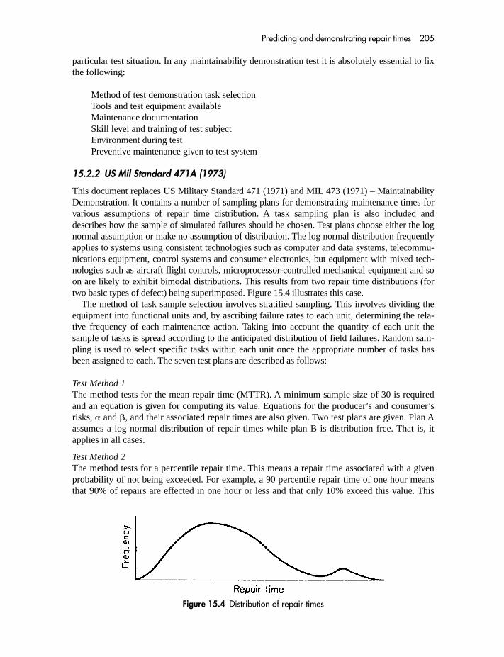
Predicting and demonstrating repair times 205
particular test situation. In any maintainability demonstration test it is absolutely essential to fixthe following:
Method of test demonstration task selectionTools and test equipment availableMaintenance documentationSkill level and training of test subjectEnvironment during testPreventive maintenance given to test system
15.2.2 US Mil Standard 471A (1973)
This document replaces US Military Standard 471 (1971) and MIL 473 (1971) – MaintainabilityDemonstration. It contains a number of sampling plans for demonstrating maintenance times forvarious assumptions of repair time distribution. A task sampling plan is also included anddescribes how the sample of simulated failures should be chosen. Test plans choose either the lognormal assumption or make no assumption of distribution. The log normal distribution frequentlyapplies to systems using consistent technologies such as computer and data systems, telecommu-nications equipment, control systems and consumer electronics, but equipment with mixed tech-nologies such as aircraft flight controls, microprocessor-controlled mechanical equipment and soon are likely to exhibit bimodal distributions. This results from two repair time distributions (fortwo basic types of defect) being superimposed. Figure 15.4 illustrates this case.
The method of task sample selection involves stratified sampling. This involves dividing theequipment into functional units and, by ascribing failure rates to each unit, determining the rela-tive frequency of each maintenance action. Taking into account the quantity of each unit thesample of tasks is spread according to the anticipated distribution of field failures. Random sam-pling is used to select specific tasks within each unit once the appropriate number of tasks hasbeen assigned to each. The seven test plans are described as follows:
Test Method 1The method tests for the mean repair time (MTTR). A minimum sample size of 30 is requiredand an equation is given for computing its value. Equations for the producer’s and consumer’srisks, � and �, and their associated repair times are also given. Two test plans are given. Plan Aassumes a log normal distribution of repair times while plan B is distribution free. That is, itapplies in all cases.
Test Method 2The method tests for a percentile repair time. This means a repair time associated with a givenprobability of not being exceeded. For example, a 90 percentile repair time of one hour meansthat 90% of repairs are effected in one hour or less and that only 10% exceed this value. This
Figure 15.4 Distribution of repair times

206 Reliability, Maintainability and Risk
test assumes a log normal distribution of repair times. Equations are given for calculating thesample size, the risks and their associated repair times.
Test Method 3The method tests the percentile value of a specified repair time. It is distribution free and there-fore applies in all cases. For a given repair time, values of sample size and pass criterion arecalculated for given risks and stated pass and fail percentiles. For example, if a median MTTRof 30 min is acceptable, and if 30 min as the 25th percentile (75% of values are greater) isunacceptable, the test is established as follows. Producer’s risk is the probability of rejectionalthough 30 min is the median, and consumer’s risk is the probability of acceptance although30 min is only the 25th percentile. Let these both equal 10%. Equations then give the value ofsample size as 23 and the criterion as 14. Hence if more than 14 of the observed values exceed30 min the test is failed.
Test Method 4The method tests the median time. The median is the value, in any distribution, such that 50%of values exceed it and 50% do not. Only in the normal distribution does the median equal themean. A log normal distribution is assumed in this test which has a fixed sample size of 20. Thetest involves comparing log MTTR in the test with log of the median value required in a givenequation.
Test Method 5The method tests the ‘Chargeable Down Time per Flight’. This means the down time attributableto failures as opposed to passive maintenance activities, test-induced failures, modifications, etc.It is distribution free with a minimum sample size of 50 and can be used, indirectly, to demon-strate availability.
Test Method 6The method is applicable to aeronautical systems and tests the ‘Man-hour Rate’. This is defined as
Actual data are used and no consumer or producer risks apply.
Test Method 7This is similar to Test Method 6 and tests the man-hour rate for simulated faults. There is aminimum sample size of 30.
Test Methods 1–4 are of a general nature whereas Methods 5–7 have been developed withaeronautical systems in mind. In applying any test the risks must be carefully evaluated. Thereis a danger, however, of attaching an importance to results in proportion to the degree of caregiven to the calculations. It should therefore be emphasized that attention to the items listed inSection 15.2.1 in order to ensure that they reflect the agreed maintenance environment is ofequal if not greater importance.
15.2.3 Data collection
It would be wasteful to regard the demonstration test as no more than a means of determiningcompliance with a specification. Each repair is a source of maintainability design evaluationand a potential input to the manual. Diagnostic instructions should not be regarded as staticbut be updated as failure information accrues. If the feedback is to be of use, it is necessary to
Total chargeable Maintenance Man-hours
Total Demonstration Flight Hours

Predicting and demonstrating repair times 207
record each repair with the same detail as is called for in field reporting. The different repairelements of diagnosis, replacement, access, etc. should be listed separately, together withdetails of tools and equipment used. Demonstration repairs are easier to control than fieldmaintenance and should therefore be better documented.
In any maintainability (or reliability) test the details should be fully described in order tominimize the possibilities of disagreement. Both parties should understand fully the quantitativeand qualitative risks involved.

16 Quantified reliability centredmaintenance
16.1 WHAT IS QRCM?
Quantitative Reliability Centred Maintenance (QRCM) involves calculations to balance the costof excessive maintenance against that of the unavailability arising from insufficient maintenance.The following example illustrates one of the techniques which will be dealt with in this chapter.
Doubling the proof-test interval of a shutdown system on an off-shore productionplatform might lead to an annual saving of 2 man-days (say £2000). The cost in increasedproduction unavailability might typically be calculated as 8 � 10�7 in which case the losswould be 8 � 10�7 � say £10 (per barrel) � say 50 K (barrels) � 365 (days) � £146. Inthis case the reduction in maintenance is justified as far as cost is concerned.
QRCM is therefore the use of reliability techniques to optimize:
� Replacement (discard) intervals� Spares holdings� Proof-test intervals� Condition monitoring
The first step in planning any QRCM strategy is to identify the critical items affecting plantunavailability since the greater an item’s contribution to unavailability (or hazard) the morepotential savings are to be made from reducing its failure rate.
Reliability modelling techniques lend themselves to this task in that they allow comparativeavailabilities to be calculated for a number of maintenance regimes. In this way the costs associatedwith changes in maintenance intervals, spares holdings and preventive replacement (discard) timescan be compared with the savings achieved.
An important second step is to obtain site specific failure data. Although QRCM techniquescan be applied using GENERIC failure rates and down times, there is better precision from sitespecific data. This is not, however, always available and published data sources (such asFARADIP.THREE) may have to be used. These are described in Chapter 4.
Because of the wide range of generic failure rates, plant specific data is preferred and anaccurate plant register goes hand in hand with this requirement. Plant registers are often out ofdate and should be revised at the beginning of a new QRCM initiative. Thought should begiven to a rational, hierarchical numbering for plant items which will assist in sorting likeitems, related items and items with like replacement times for purposes of maintenance andspares scheduling.
Good data is essential because, in applying QRCM, it is vital to take account of the way inwhich failures are distributed with time. We need to know if the failure rate is constant or

Quantified reliability centred maintenance 209
whether it is increasing or decreasing. Preventive replacement (discard), for example, is onlyjustified if there is an increasing failure rate.
16.2 THE QRCM DECISION PROCESS
The use of these techniques depends upon the failure distribution, the degree of redundancy andwhether the cost of the maintenance action is justified by the saving in operating costs, safety orenvironmental impact. Figure 16.1 is the QRCM decision algorithm which can be used duringFMEA. As each component failure is considered the QRCM algorithm provides the logic whichleads to the use of each of the techniques.
Using Figure 16.1 consider an unrevealed failure which, if it coincides with some other failure,leads to significant consequences such as the shutdown of a chemical plant. Assume that there is nomeasurable check whereby the failure can be pre-empted. Condition monitoring is not thereforeappropriate. Assume, also, that the failure rate is not increasing therefore preventive discard cannotbe considered. There is, however, an optimum proof-test interval whereby the cost of proof testcan be balanced against the penalty cost of the coincident failures.
Is the failurerevealed or unrevealed
DO NOTHING
UnrevealedRevealed Consideroptimumspares
In combination withother failures, are theconsequences trivial?
Is there ameasurabledegradationparameter?
Is there ameasurabledegradationparameter?
Are the consequences
trivial?
Is thefailure rateincreasing?
Calculateoptimumproof test
Calculatepreventive
replacement
Carry outcondition
monitoring
Is thefailure rateincreasing?
Calculatepreventive
replacementand optimum
proof testTrivial implies that the financial,safety or environmental penaltydoes not justify the cost of theproposed maintenance
Carry outcondition
monitoringand
calculateoptimumproof test
All
No
No
No
No
No
No Yes
Yes Yes
Yes
Yes Yes
Figure 16.1 The QRCM decision algorithm

210 Reliability, Maintainability and Risk
16.3 OPTIMUM REPLACEMENT (DISCARD)
Specific failure data is essential for this technique to be applied sensibly. There is no genericfailure data describing wearout parameters which would be adequate for making discarddecisions. Times to failure must be obtained for the plant items in question and the Weibulltechniques described in Chapter 6 applied. Note that units of time may be hours, cycles,operations or any other suitable base.
Only a significant departure of the shape parameter from (� � 1) justifies considering discard.If � � 1 then there is no justification for replacement or even routine maintenance. If, on the
other hand, � � 1 then there may be some justification for considering a preventive replacementbefore the item has actually failed. This will only be justified if the costs associated with anunplanned replacement (due to failure) are greater than those of a planned discard/replacement.
If this is the case then it is necessary to calculate:
(a) the likelihood of a failure (i.e. 1 � exp(�t/�)�) in a particular interval times the cost of theunplanned failure.
(b) the cost of planned replacements during that interval.
The optimum replacement interval which minimizes the sum of the above two costs can thenbe found. Two maintenance philosophies are possible:
� Age replacement� Block replacement
For the Age replacement case, an interval starts at time t � 0 and ends either with a failure or witha replacement at time t � T, whichever occurs first. The probability of surviving until time t � T isR(T) thus the probability of failing is 1 � R(T). The average duration of all intervals is given by:
Thus the cost per unit time is:
where £u is the cost of unplanned outage (i.e. failure) and £p is the cost of a planned replacement.For the Block replacement case, replacement always occurs at time t � T despite the possibility
of failures occurring before time t � T. For this case the cost per unit time is:
(£u � T)/MTBF � T £p/T � £u/MTBF £p/T
Note that, since the failure rate is not constant (� � 1), the MTBF used in the formula variesas a function of T.
There are two maintenance strategies involving preventive replacement (discard):
(a) If a failure occurs replace it and then wait the full interval before replacing again. This isknown as AGE replacement.
(b) If a failure occurs replace it and nevertheless replace it again at the expiration of the exist-ing interval. This is known as BLOCK replacement.
[£u � (1 � R(T )) £p � R(T )]
�T
0
R(t) dt
�T
0
R(t) dt
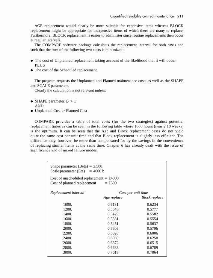
Quantified reliability centred maintenance 211
AGE replacement would clearly be more suitable for expensive items whereas BLOCKreplacement might be appropriate for inexpensive items of which there are many to replace.Furthermore, BLOCK replacement is easier to administer since routine replacements then occurat regular intervals.
The COMPARE software package calculates the replacement interval for both cases andsuch that the sum of the following two costs is minimized:
� The cost of Unplanned replacement taking account of the likelihood that it will occur.PLUS
� The cost of the Scheduled replacement.
The program requests the Unplanned and Planned maintenance costs as well as the SHAPEand SCALE parameters.
Clearly the calculation is not relevant unless:
� SHAPE parameter, � � 1AND
� Unplanned Cost � Planned Cost
COMPARE provides a table of total costs (for the two strategies) against potentialreplacement times as can be seen in the following table where 1600 hours (nearly 10 weeks)is the optimum. It can be seen that the Age and Block replacement cases do not yieldquite the same cost per unit time and that Block replacement is slightly less efficient. Thedifference may, however, be more than compensated for by the savings in the convenienceof replacing similar items at the same time. Chapter 6 has already dealt with the issue ofsignificance and of mixed failure modes.
Shape parameter (Beta) � 2.500Scale parameter (Eta) � 4000 h
Cost of unscheduled replacement � £4000Cost of planned replacement � £500
Replacement interval Cost per unit timeAge replace Block replace
1000. 0.6131 0.62341200. 0.5648 0.57771400. 0.5429 0.55821600. 0.5381 0.55541800. 0.5451 0.56372000. 0.5605 0.57962200. 0.5820 0.60062400. 0.6080 0.62502600. 0.6372 0.65152800. 0.6688 0.67893000. 0.7018 0.7064

212 Reliability, Maintainability and Risk
16.4 OPTIMUM SPARES
There is a cost associated with carrying spares, namely capital depreciation, space,maintenance, etc. In order to assess an optimum spares level it is necessary therefore tocalculate the unavailability which will occur at each level of spares holding. This willdepend on the following variables:
� Number of spares held� Failure rate of the item� Number of identical items in service� Degree of redundancy within those items� Lead time of procurement of spares� Replacement (Unit Down Time) time when an item fails
This relationship can be modelled by means of Markov state diagram analysis and was fullydescribed in Chapter 14 (Section 14.2.6).
It should be noted that, as the number of spares increases, there is a diminishing return interms of improved unavailability until the so-called infinite spares case is reached. This iswhere the unavailability is dominated by the repair time and thus increased spares holdingbecomes ineffectual. At this point, only an improvement in repair time or in failure rate canincrease the availability.
The cost of unavailability can be calculated for, say, zero spares. The cost saving in reducedunavailability can then be compared with the cost of carrying one spare and the processrepeated until the optimum spares level is assessed.
The COMPARE package allows successive runs to be made for different spares levels.Figure 14.5 shows the Markov state diagram for 4 units with up to 2 spares.
16.5 OPTIMUM PROOF TEST
In the case of redundant systems where failed redundant units are not revealed then the option ofperiodic proof test arises. Although the failure rate of each item is constant, the system failurerate actually increases.
The Unavailability of a system can be calculated using the methods described in Chapter 8. Itis clearly dependent partly on the proof-test interval which determines the down time of a failed(dormant) redundant item.
The technique involves calculating an optimum proof-test interval for revealing dormant fail-ures. It seeks to trade off the cost of the proof test (i.e. preventive maintenance) against thereduction in unavailability.
It applies where coincident dormant failures cause unavailability. An example would be thefailure to respond of both a ‘high’ alarm and a ‘high high’ signal.
The unavailability is a function of the instrument failure rates and the time for which dormantfailures persist. The more frequent the proof test, which seeks to identify the dormant failures,then the shorter is the down time of the failed items.
Assume that the ‘high’ alarm and ‘high high’ signal represent a duplicated redundantarrangement. Thus, one instrument may fail without causing plant failure (shutdown).
It has already been shown that the reliability of the system is given by:
R(t) � 2 e�t � e�2t

Quantified reliability centred maintenance 213
Thus the probability of failure is 1 � R(t)
� 1 � 2 e�t e�2t
If the cost of an outage (i.e. lost production) is £u then the expected cost, due to outage, is:
� (1 � 2 e�t e�2t) � £u
Now consider the proof test, which costs £p per visit. If the proof-test interval is T then theexpected cost, due to preventive maintenance, is:
� (2 e�t � e�2t) � £p
The total cost per time interval is thus:
� [(1 � 2 e�t e�2t) � £u] [(2 e�t � e�2t) � £p]
The average length of each interval is
� 3/2 � 2/ e�T 1/2 e�2T
The total cost per unit time can therefore be obtained by dividing the above expression into thepreceding one.
The minimum cost can be found by tabulating the cost against the proof-test interval (T). Inthe general case the total cost per unit time is:
Again, the COMPARE package performs this calculation and provides an optimum interval(approximately 3 years) as can be seen in the following example.
�[(1 � R(T)) � £u] [R(T ) � £p]
�T
0R(t) dt
�T
0R(t) dt
Total number of units � 2Number of units required � 1MTBF of a single unit � 10.00 years
Cost of unscheduled outage � £2000Cost of a planned visit � £100
Proof-test interval Cost per unit time
1.000 117.61.700 86.882.400 78.983.100 77.793.800 79.184.500 81.655.200 84.565.900 87.606.600 90.617.300 93.518.000 96.28

214 Reliability, Maintainability and Risk
16.6 CONDITION MONITORING
Many failures do not actually occur spontaneously but develop over a period of time. It follows,therefore, that if this gradual ‘degradation’ can be identified it may well be possible to pre-emptthe failure. Overhaul or replacement are then realistic options. During the failure mode analysisit may be possible to determine parameters which, although not themselves causing a hazard orequipment outage, are indicators of the degradation process.
In other words, the degradation parameter can be monitored and action taken to prevent fail-ure by observing trends. Trend analysis would be carried out on each of the measurements inorder to determine the optimum point for remedial action.
It is necessary for there to be a reasonable time period between the onset of the measurabledegradation condition and the actual failure. The length (and consistency) of this period willdetermine the optimum inspection interval.
There are a number of approaches to determining the inspection interval. Methods involvinga gradual increase in interval run the risk of suffering the failure. This may be expensive or haz-ardous. Establishing the interval by testing, although safer, is expensive, may take time andrelies on simulated operating environments. However, in practice, a sensible mixture of experi-ence and data can lead to realistic intervals being chosen. By concentrating on a specific failuremode (say valve diaphragm leakage) and by seeking out those with real operating experience itis possible to establish realistic times. Even limited field and test data will enhance the decision.
The following list provides some examples of effects which can be monitored:
� regular gas and liquid emission leak checks� critical instrumentation parameter measurements (gas, fire, temp, level, etc.)� insulation resistivity� vibration measurement and analysis of characteristics� proximity analysis� shock pulse monitoring� acoustic emission� corrosive states (electro-chemical monitoring)� dye penetration� spectrometric oil analysis� electrical insulation� hot spots� surface deterioration� state of lubrication and lubricant� plastic deformation� balance and alignment.

17 Systematic failures, especially software
The qualitative techniques dealt with so far in this book refer largely to catastrophic hardwarefailures. The term ‘random hardware failures’ covers the constant failure rate aspect of the bath-tub and the term ‘dependent failures’ embraces the common cause aspects dealt with earlier.
Systematic failures, however, are generally considered to be in addition to those which wequantify by means of failure rate (or even Weibull) methods. Since they do not relate to past‘failure’ data, it follows that it is very difficult to justify their being predicted by the modellingtechniques we have considered so far.
Therefore, qualitative measures are described in the hope that they will minimize thesesystematic failures. In Chapter 22, which deals specifically with safety-related systems, theconcept of integrity levels will be introduced. This involves prescribing varying levels ofrigour for these qualitative measures, according to the degree of integrity required.
The following sections summarize these defences with particular reference to software-relatedfailure.
17.1 PROGRAMMABLE DEVICES
There has been an accelerating growth, since the 1970s, in the use of programmable devices.They have made a significant impact on methods of electronic circuit design. The main effecthas been to reduce the number of different circuit types by the use of computer architecture.Coupled with software programming, this provides the individual circuit features previouslyachieved by differences in hardware. The word ‘software’ refers to the instructions needed toenable a programmable device to function, including the associated hierarchy of documentsrequired to produce that code. This use of programming at the circuit level, now common withmost industrial and consumer products, brings with it some associated quality and reliabilityproblems. When applied to microprocessors at the circuit level, the programming, which issemi-permanent and usually contained in ROM (Read Only Memory), is known as Firmware.The necessary increase in function density of devices in order to provide the large quantities ofmemory in small packages has matched this trend.
Computing and its associated software was once seen in three broad categories:
1. Mainframe computing: involving systems which provide a very large number of termi-nals and support a variety of concurrent tasks. Typical functions are interactive desktopterminals or bank terminals. Such systems were once characterized by the available diskand tape storage but, nowadays, even PCs have memory capacity far in excess of 1990’smainframes.

216 Reliability, Maintainability and Risk
2. Minicomputing: was a term used for smaller, more compact, systems whose CPUs may wellhave dealt with the same word length as a mainframe. The principal difference was in thearchitecture of the main components and, also, in the way in which they communicated withthe peripherals.
3. Microprocessing: the advent of the microcomputer brought many of the mainframe/minicomputer functions to the desktop and it is this area where speed and memory haveincreased most dramatically.
The microprocessor has now largely replaced both the minicomputer and the mainframe fornormal industrial applications.
Categorizing of programmable devices is now more subtle and involves differences in softwareapproach as much as in hardware architecture. We now need to consider the following differences:
1. Mainframe–MinicomputerPhysical size has become largely irrelevant. These devices carry out computational and datahandling tasks using proprietary software packages. They also permit programming in thewhole range of complex branching languages. Real time control is possible by interfacingwith instrumentation and with field devices.
2. Programmable Logic Controllers (PLCs)Although similar in construction to the above devices, there is a more consistent architecturewith the accent on providing input and output ports which allow large amounts of ‘data in’and ‘command out’ capability in analogue, digital and loop modes. Languages are usuallyproprietary to the device in question and are frequently much more simple than the well-known branching programming languages. Thus, programming is simplified and the oppor-tunity for errors in code design is significantly reduced.
3. Embedded microcomputingIn this case the computer architecture is provided by processor and memory LSI chips.Individual designs are carried out at printed board level and programming can be at assembler(machine code) level as well as by means of some of the traditional programming languages.On one hand there is total flexibility of design but, on the other, opportunities for timing-relatedcircuit problems, as well as code design errors, are much greater.
From the safety-integrity and from the reliability point of view, there are both advantagesand disadvantages arising from programmable design solutions. The relative magnitude ofthe advantages and disadvantages will vary according to the type of device (as describedearlier):
Reliability/integrity Advantages Reliability/integrity Disadvantages
� Fewer different types of hardware � Difficult to ‘inspect’ software for errors� Consistent architectures (CPU/bus/I-O) � Test involves a limited sample of � Common approach to hardware design execution possibilities� Easier to support several versions � Control of changes is more complicated
in the field and more critical� Simpler to implement modifications � Difficult to impose programming
‘standard approaches’� Very difficult to predict meaningful
‘failure rates’ of software-related systematic failures

Systematic failures, especially software 217
17.2 SOFTWARE-RELATED FAILURES
The question arises as to how a software failure is defined. Unlike hardware, there is no phys-ical change associated with a unit that is ‘functional’ at one moment and ‘failed’ at the next.Software failures are in fact errors which, owing to the complexity of a computer program, donot become evident until the combination of conditions brings the error to light. The effect isthen the same as any other failure. Unlike the hardware Bathtub, there is no wearout character-istic but only a continuing burn-in. Each time that a change to the software is made the errorrate is likely to rise, as shown in Figure 17.1. As a result of software errors there has been, forsome time, an interest in developing methods of controlling the activities of programmers andof reducing software complexity by attempts at standardization.
Figure 17.2 illustrates the additional aspect of software failures in programmable systems. Itintroduces the concept of Fault/Error/Failure. Faults may occur in both hardware and software.Software faults, often known as bugs, will appear as a result of particular portions of code beingused for the first time under a particular set of circumstances.
Errorrate Change
Time
WearoutRandom
Over-stress
Design
Process
Hardwarefault
Undetected
Design
Data
HumanSoftware
fault
Specification
e.m.c.
Recovery
SoftwareError No
failure
System failure
Figure 17.1 Software error curve
Figure 17.2

218 Reliability, Maintainability and Risk
The presence of a fault in a programmed system does not necessarily result in either an erroror a failure. A long time may elapse before that code is used under the circumstances whichlead to failure.
A fault (bug) may lead to an error, which occurs when the system reaches an incorrect state.That is, a bit, or bits, takes an incorrect value in some store or highway.
An error may propagate to become a failure if the system does not contain error-recoverysoftware capable of detecting and eliminating the error.
Failure, be it for hardware or software reasons, is the termination of the ability of an item toperform the function specified.
It should be understood that the term ‘software’ refers to the complete hierarchy of documenta-tion which defines a programmable system. This embraces the Requirements Specification, DataSpecifications, Subsystem Specifications and Module definitions, as well as the Flowcharts,Listings and Media which are often thought of as comprising the entire software.
Experience shows that less than 1% of software failures result from the actual ‘production’ ofthe firmware. This is hardly surprising since the act of inputting code is often self-checking anderrors are fairly easy to detect. This leaves the design and coding activities as the source offailures. Within these, less than 50% of errors are attributed to the coding activity. Softwarereliability is therefore inherent in the design process of breaking down the requirements intosuccessive levels of specification.
17.3 SOFTWARE FAILURE MODELLING
Numerous attempts have been made to design models which enable software failure rates to bepredicted from the initial failures observed during integration and test or from parameters suchas the length and nature of the code. The latter suffers from the difficulty that, in software, thereare no elements (as with hardware components) with failure characteristics which can be takenfrom experience and used for predictive purposes. This type of prediction is therefore unlikelyto prove successful. The former method, of modelling from the early failures, suffers from adifficulty which is illustrated by this simple example. Consider the following failure patternbased on 4 days of testing:
Day 1 10 failuresDay 2 9 failuresDay 3 8 failuresDay 4 7 failures
To predict, from these data, when 6 failures per day will be observed is not difficult, but what isrequired is to know when the failure rate will be 10�4 or perhaps 10�5. It is not certain that theinformation required is in fact contained within the data. Figure 17.3 illustrates the coarseness
Figure 17.3

Systematic failures, especially software 219
of the data and the fact that the tail of the distribution is not well defined and by no meansdetermined by the shape of the left-hand end.
A number of models have been developed. They rely on various assumptions concerning thenature of the failure process, such as the idea that failure rate is determined by the number ofpotential failures remaining in the program. These are by no means revealed solely by thepassage of calendar time, since repeated executions of the same code will not usually revealfurther failures.
Present opinion is that no one model is better than any other, and it must be said that, in anycase, an accurate prediction only provides a tool for scheduling rather than a long-term fieldreliability assessment. The models include:
� Jelinski Moranda: This assumes that failure rate is proportional to the remaining faultcontent. Remaining faults are assumed to be equally likely to occur.
� Musa: Program execution rather than calendar time is taken as the variable.� Littlewood Verall: Assumes successive execution time between failures to be an exponen-
tially distributed random variable.� Structured Models: These attempt to break software into subunits. Rules for switching
between units and for the failure rate of each unit are developed.� Seeding and Tagging: This relies on the injection of known faults into the software. The suc-
cess rate of debugging of the known faults is used to predict the total population of failuresby applying the ratio of success to the revealed non-seeded failures. For this method to besuccessful one has to assume that the seeded failures are of the same type as the unknownfailures.
Clearly, the number of variables involved is large and their relationship to failure rate farfrom precise. It is the author’s view that, currently, qualitative activities in Software QualityAssurance are more effective than attempts at prediction.
17.4 SOFTWARE QUALITY ASSURANCE
Software QA, like hardware QA, is aimed at preventing failures. It is based on the observationthat software failures are predominantly determined by the design. Experience in testing real-time software controlled systems shows that 50% of software ‘bugs’ result from unforeseencombinations of real-time operating events which the program instructions cannot accommo-date. As a result, the algorithm fails to generate a correct output or instruction and the systemfails.
Software QA is concerned with:
Organization of Software QA effort (Section 17.4.1)Documentation Controls (17.4.2)Programming Standards (17.4.3)Design Features (17.4.4)Code Inspections and Walkthroughs (17.4.5)Integration and Test (17.4.6)
The following sections outline these areas and this chapter concludes with a number of checklistquestions suitable for audit or as design guidelines.

220 Reliability, Maintainability and Risk
17.4.1 Organization of Software QA
There needs to be an identifiable organizational responsibility for Software QA. The importantpoint is that the function can be identified. In a small organization, individuals often carry out anumber of tasks. It should be possible to identify written statements of responsibility forSoftware QA, the maintenance of standards and the control of changes.
There should be a Quality Manual, Quality Plans and specific Test Documents controlled byQA independently of the project management. They need not be called by those names and maybe contained in other documents. It is the intent which is important. Main activities shouldinclude:
Configuration ControlLibrary of Media and DocumentationDesign ReviewAuditingTest Planning
17.4.2 Documentation controls
There must be an integrated hierarchy of Specification/Documents which translates the func-tional requirements of the product through successive levels of detail to the actual source code.In the simplest case this could be satisfied by:
A Functional description andA Flowchart or set of High-Level Statements andA Program listing.
In more complex systems there should be a documentation hierarchy. The design must focusonto a user requirements specification which is the starting point in a top-down approach.
In auditing software it is important to look for such a hierarchy and to establish a diagramsimilar to Figure 17.4, which reflects the product, its specifications and their numbering system.Failure to obtain this information is a sure indicator that software is being produced with lessthan adequate controls. Important documents are:
� User requirements specification: Describes the functions required of the system. It should beunambiguous and complete and should describe what is required and not how it is to beachieved. It should be quantitative, where possible, to facilitate test planning. It states what isrequired and must not pre-empt and hence constrain the design.
� Functional specification: Whereas the User requirements specification states what is required,the Functional specification outlines how it will be achieved. It is usually prepared by thedeveloper in response to the requirements.
� Software design specification: Takes the above requirements and, with regard to the hard-ware configuration, describes the functions of processing which are required and addressessuch items as language, memory requirements, partitioning of the program into accessiblesubsystems, inputs, outputs, memory organization, data flow, etc.
� Subsystem specification: This should commence with a brief description of the subsystemfunction. Interfaces to other subsystems may be described by means of flow diagrams.
� Module specification: Treating the module as a black box, it describes the interfaces with therest of the system and the functional performance as perceived by the rest of the software.

Systematic failures, especially software 221
Figure 17.4 The design cycle

222 Reliability, Maintainability and Risk
� Module definition: Describes the working of the software in each module. It should includethe module test specification, stipulating details of input values and the combinations whichare to be tested.
� Charts and diagrams: A number of techniques are used for charting or describing a module. Themost commonly known is the flowchart, shown in Figure 17.5. There are, however, alternatives,particularly in the use of high-level languages. These involve diagrams and pseudo-code.
� Utilities specification: This should contain a description of the hardware requirements,including the operator interface and operating system, the memory requirements, processorhardware, data communications and software support packages.
� Development notebooks: An excellent feature is the use of a formal development notebook.Each designer opens a loose-leaf file in which is kept all specifications, listings, notes,change documentation and correspondence pertaining to that project.
Change controlAs with hardware, the need to ensure that changes are documented and correctly applied to allmedia and program documents is vital. All programs and their associated documents shouldtherefore carry issue numbers. A formal document and software change procedure is required(see Figure 17.6) so that all change proposals are reviewed for their effect on the total system.
17.4.3 Programming standards
The aim of structured programming is to reduce program complexity by using a library ofdefined structures wherever possible. The human brain is not well adapted to retaining randominformation and sets of standard rules and concepts substantially reduce the likelihood of error.A standard approach to creating files, polling output devices, handling interrupt routines, etc.constrains the programmer to use the proven methods. The use of specific subroutines is a fur-ther step in this direction. Once a particular sequence of program steps has been developed inorder to execute a specific calculation, then it should be used as a library subroutine by the restof the team. Re-inventing the wheel is both a waste of time and an unnecessary source of failureif an error-free program has already been developed.
Figure 17.5 Flowchart

Systematic failures, especially software 223
A good guide is 30–60 lines of coding plus 20 lines of comment. Since the real criterionis that the module shall be no larger than to permit a total grasp of its function (that is, it isperceivable), it is likely that the optimum size is a line print page (3 at most).
The use of standard sources of information is of immense value. Examples are:
Standard values for constantsCode Templates (standard pieces of code for given flowchart elements)Compilers
The objective is to write clear, structured software, employing well-defined modules whosefunctions are readily understood. There is no prize for complexity.
There are several methods of developing the module on paper. They include:
Flow DiagramsHierarchical DiagramsStructured Box DiagramsPseudo-code
Authorizedocumentation
change
Modify sourcecode
Software changeproposal
Review proposal
Review documentation
Document modificationproposal
Compile newobject media
Simulationsand packages
Run and verify
Corrections
Modify build staterecords and producesecondary document
masters
Release software
Release andDistribute
Software QA
Proofcheck
Modify softwareBuild state records
Produce secondarymasters of software
media
Figure 17.6 Software change and documentation procedure

224 Reliability, Maintainability and Risk
17.4.4 Fault-tolerant design features
Fault tolerance can be enhanced by attention to a number of design areas. These features include:
� Use of redundancy, which is expensive. The two options are Dual Processing and AlternatePath (Recovery Blocks).
� Use of error-checking software involving parity bits or checksums together with routines forcorrecting the processing.
� Timely display of fault and error codes.� Generous tolerancing of timing requirements.� Ability to operate in degraded modes.� Error confinement. Programming to avoid error proliferation or, failing that, some form of
recovery.� Watchdog timer techniques involve taking a feedback from the microprocessor and, using
that clocked rate, examining outputs to verify that they are dynamic and not stuck in onestate. The timer itself should be periodically reset.
� Faults in one microprocessor should not be capable of affecting another. Protection by meansof buffers at inputs and outputs is desirable so that a faulty part cannot pull another part intoan incorrect state. Software routines for regular checking of the state (high or low) of eachpart may also be used.
� Where parts of a system are replicated the use of separate power supplies can be considered,especially since the power supply is likely to be less reliable than the replicated processor.
17.4.5 Reviews
There are two approaches to review of code:
1. Code Inspection where the designer describes the overall situation and the module functionsto the inspection team. The team study the documentation and, with the aid of previous faulthistories, attempt to code the module. Errors are sought and the designer then carries out anyrework, which is then re-inspected by the team.
2. The Structured Walkthrough in which the designer explains and justifies each element ofcode until the inspection team is satisfied that they agree and understand each module.
17.4.6 Integration and test
There are various types of testing which can be applied to software:
� Dynamic Testing: This involves executing the code with real data and I/O. At the lowest levelthis can be performed on development systems as is usually the case with Module Testing.As integration and test proceeds, the dynamic tests involve more of the actual equipmentuntil the functional tests on the total equipment are reached. Aids to dynamic testing includeautomatic test beds and simulators which are now readily available.
� Path Testing: This involves testing each path of the software. In the case of flowcharteddesign there are techniques for ‘walking through’ each path and determining a test. It is diffi-cult, in a complex program, to be sure that all combinations have been checked. In fact thenumber of combinations may be too high to permit all paths to be tested.
� Software Proving by Emulation: An ‘intelligent’ communications analyser or other simulatorhaving programmable stimulus and response facilities is used to emulate parts of the system

Systematic failures, especially software 225
not yet developed. In this way the software can be made to interact with the emulator whichappears as if it were the surrounding hardware and software. Software testing can thus pro-ceed before the total system is complete.
� Functional Testing: The ultimate empirical test is to assemble the system and to test everypossible function. This is described by a complex test procedure and should attempt to coverthe full range of environmental conditions specified.
� Load Testing: The situation may exist where a computer controls a number of smallermicroprocessors, data channels or even hard-wired equipment. The full quantity of theseperipheral devices may not be available during test, particularly if the system is designedfor expansion. In these cases, it is necessary to simulate the full number of inputs by meansof a simulator. A further micro or minicomputer may well be used for this purpose. Testsoftware will then have to be written which emulates the total number of devices and sendsand receives data from the processor under test.
Be most suspicious of repeated slip in a test programme. This is usually a symptom that thetest procedure is only a cover for debug. Ideally, a complete error-free run of the test procedureis needed after debug, although this is seldom achieved in practice with large systems.
The practice of pouring in additional personnel to meet the project schedule is ineffective.The division of labour, below module level, actually slows down the project.
17.5 MODERN/FORMAL METHODS
The traditional Software QA methods, described in the previous section, are essentiallyopen-ended checklist techniques. They have been developed over the last 15 years but wouldbe greatly enhanced by the application of more formal and automated methods. The mainproblem with the existing open-ended techniques is that they provide no formal measures asto how many of the hidden errors have been revealed.
The term Formal Methods is much used and much abused. It covers a number of methodologiesand techniques for specifying and designing systems, both non-programmable and programmable.They can be applied throughout the life cycle including the specification stage and the softwarecoding itself.
The term is used here to describe a range of mathematical notations and techniques appliedto the rigorous definition of system requirements which can then be propagated into the subse-quent design stages. The strength of formal methods is that they address the requirements atthe beginning of the design cycle. One of the main benefits of this is that formalism applied atthis early stage may lead to the prevention, or at least early detection, of incipient errors. Thecost of errors revealed at this stage is dramatically less than if they are allowed to persist untilcommissioning or even field use. This is because the longer they remain undetected the moreserious and far reaching are the changes required to correct them.
The three major quality problems, with software, are illustrated in Figure 17.7. First, thestatement of requirements is in free language and thus the opportunity for ambiguity, error andomission is at a maximum. The very free language nature of the requirements makes it impos-sible to apply any formal or mathematical review process at this stage. It is well known that themajority of serious software failures originate in this part of the design cycle. Second, thesource code, once produced, can only be reviewed by open-ended techniques as described inSection 17.4.4. Again, the discovery of ten faults gives no clue as whether one, ten or 100remain. Third, the use of the software (implying actual execution of the code) is effectively avery small sample of the execution paths and input/output combinations which are possible in
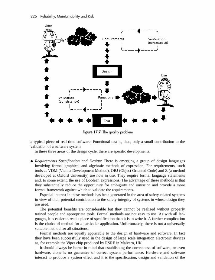
226 Reliability, Maintainability and Risk
a typical piece of real-time software. Functional test is, thus, only a small contribution to thevalidation of a software system.
In these three areas of the design cycle, there are specific developments:
� Requirements Specification and Design: There is emerging a group of design languagesinvolving formal graphical and algebraic methods of expression. For requirements, suchtools as VDM (Vienna Development Method), OBJ (Object Oriented Code) and Z (a methoddeveloped at Oxford University) are now in use. They require formal language statementsand, to some extent, the use of Boolean expressions. The advantage of these methods is thatthey substantially reduce the opportunity for ambiguity and omission and provide a moreformal framework against which to validate the requirements.
Especial interest in these methods has been generated in the area of safety-related systemsin view of their potential contribution to the safety-integrity of systems in whose design theyare used.
The potential benefits are considerable but they cannot be realized without properlytrained people and appropriate tools. Formal methods are not easy to use. As with all lan-guages, it is easier to read a piece of specification than it is to write it. A further complicationis the choice of method for a particular application. Unfortunately, there is not a universallysuitable method for all situations.
Formal methods are equally applicable to the design of hardware and software. In factthey have been successfully used in the design of large scale integration electronic devicesas, for example the Viper chip produced by RSRE in Malvern, UK.
It should always be borne in mind that establishing the correctness of software, or evenhardware, alone is no guarantee of correct system performance. Hardware and softwareinteract to produce a system effect and it is the specification, design and validation of the
Figure 17.7 The quality problem

Systematic failures, especially software 227
system which matters. This system-wide view should also include the effects of humanbeings and the environment.
The potential for creating faults in the specification stage arises largely from the fact thatit is carried out mainly in natural language. On one hand this permits freedom of expressionand comprehensive description but, on the other, leads to ambiguity, lack of clarity and littleprotection against omission. The user communicates freely in this language which is notreadily compatible with the formalism being suggested here.
� Static Analysis: This involves the algebraic examination of source code (not its execution).Packages are available (such as MALPAS from Advantage Business Group Farnham, Surreyhttp://www.advantage-business.co.uk) which examine the code statements for such features as:
The graph structure of the pathsUnreachable codeUse of variablesDependency of variables upon each otherActual semantic relationship of variables
Consider the following piece of code:
BEGININTEGER A, B, C, D, EA: � 0NEXT: INPUT C:IF C � 0 THEN GOTO EXIT:B: � B � CD: � B/AGOTO NEXT:PRINT B, D;EXIT: END;
Static analysis will detect that:
(i) B is not initialized before use.(ii) E is never used
(iii) A is zero and is used as a divisor(iv) The PRINT B, D; command is never used because of the preceding statement.
Static analysis is extremely powerful in that it enables the outputs of the various analysersto be compared with the specification in order to provide a formal review loop between codeand specification. A further advantage is that static analysis forces the production of properspecifications since they become essential in order to make use of the analyser outputs.
Figure 17.8 shows the packages of MALPAS (one such static analysis tool). It acts on thesource code and Control flow analysis identifies the possible entry and exit points to the mod-ule, pieces of unreachable code and any infinitely looping dynamic halts. It gives an initialfeel for the structure and quality of the program. Data use analysis identifies all the inputs andoutputs of the module and checks that data is being correctly handled. For example, it checksthat each variable is initialized before being used. Information flow analysis deduces theinformation on which each output depends. The Path assessor is used to provide a measure ofthe complexity in that the number of paths through the code is reported for each procedure.

228 Reliability, Maintainability and Risk
Semantic analysis identifies the actions taken on each feasible path through a procedure. Inparticular, it rewrites imperative, step-by-step procedures into a declarative, parallel assign-ment form. The analyst can use this to provide an alternative perspective on the function ofthe procedure. The result of the analyser is to tell the analyst the actual relationship of thevariables to each other. Compliance analysis attempts to prove that a procedure satisfies aspecified condition. For example, it could be used to check that the result of the procedure‘sort’ is a sequence of items where each item is bigger than the preceding one. The reportfrom the compliance analysis identifies those input values for which the procedure will fail.
� Test Beds: During dynamic testing (involving actual execution of the code), automated ‘testbeds’ and ‘animators’ enable testing to proceed with the values of variables being displayedalongside the portions of code under test. Numerous test ‘tools’ and so-called environmentsare commercially available and continue to be developed.
17.6 SOFTWARE CHECKLISTS
17.6.1 Organization of Software QA
1. Is there a senior person with responsibility for Software QA and does he or she have adequatecompetence and authority to resolve all software matters?
2. Is there evidence of regular reviews of Software Standards?3. Is there a written company requirement for the Planning of a Software Development?4. Is there evidence of Software Training?5. Is there a Quality Manual or equivalent documents?6. Is there a system for labelling all Software Media?7. Is there a Quality Plan for each development including
Organization of the teamMilestonesCodes of PracticeQC procedures, including release
Source program
IL program
MALPAS reports
Translation
Control flow analysis reportData use analysis reportInformation flow analysis reportPath assessor reportSemantic analysis reportCompliance analysis report
1.
2.3.4.5.6.
Figure 17.8 The MALPAS suite
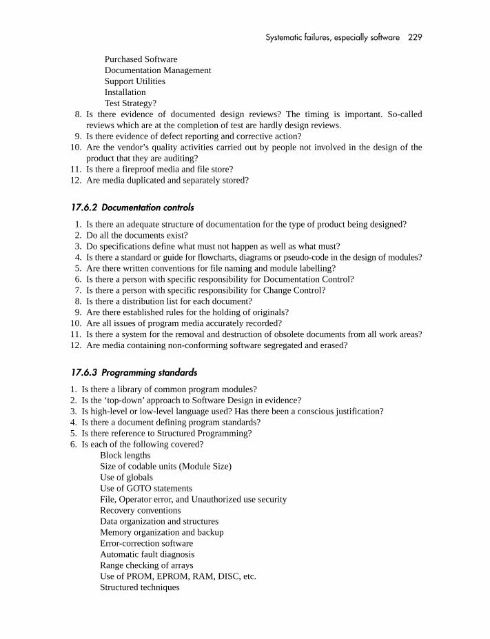
Systematic failures, especially software 229
Purchased SoftwareDocumentation ManagementSupport UtilitiesInstallationTest Strategy?
8. Is there evidence of documented design reviews? The timing is important. So-calledreviews which are at the completion of test are hardly design reviews.
9. Is there evidence of defect reporting and corrective action?10. Are the vendor’s quality activities carried out by people not involved in the design of the
product that they are auditing?11. Is there a fireproof media and file store?12. Are media duplicated and separately stored?
17.6.2 Documentation controls
1. Is there an adequate structure of documentation for the type of product being designed?2. Do all the documents exist?3. Do specifications define what must not happen as well as what must?4. Is there a standard or guide for flowcharts, diagrams or pseudo-code in the design of modules?5. Are there written conventions for file naming and module labelling?6. Is there a person with specific responsibility for Documentation Control?7. Is there a person with specific responsibility for Change Control?8. Is there a distribution list for each document?9. Are there established rules for the holding of originals?
10. Are all issues of program media accurately recorded?11. Is there a system for the removal and destruction of obsolete documents from all work areas?12. Are media containing non-conforming software segregated and erased?
17.6.3 Programming standards
1. Is there a library of common program modules?2. Is the ‘top-down’ approach to Software Design in evidence?3. Is high-level or low-level language used? Has there been a conscious justification?4. Is there a document defining program standards?5. Is there reference to Structured Programming?6. Is each of the following covered?
Block lengthsSize of codable units (Module Size)Use of globalsUse of GOTO statementsFile, Operator error, and Unauthorized use securityRecovery conventionsData organization and structuresMemory organization and backupError-correction softwareAutomatic fault diagnosisRange checking of arraysUse of PROM, EPROM, RAM, DISC, etc.Structured techniques

230 Reliability, Maintainability and Risk
Treatment of variables (that is, access)Coding formatsCode layoutComments (REM statements)Rules for module identification.
17.6.4 Design features
1. Is there evidence that the following are taken into consideration?Electrical protection (mains, airborne)Power supplies and filtersOpto isolation, buffersEarthingBattery backupChoice of processorsUse of languageRating of I/O devicesRedundancy (dual programming)Data communicationsHuman/machine interfaceLayout of hardwareHardware configuration (e.g. multidrops)Watchdog timersRAM checksError confinementError detectionError recovery.
2. Are there syntax and protocol-checking algorithms?3. Are interfaces defined such that illegal actions do not corrupt the system or lock up the
interface?4. Are all data files listed (there should be a separate list)?5. Were estimates of size and timing carried out?6. Are the timing criteria of the system defined where possible?7. Will it reconstruct any records that may be lost?8. Are there facilities for recording system state in the event of failure?9. Have acceptable degraded facilities been defined?
10. Is there a capability to recover from random jumps resulting from interference?11. Are the following adequate?
Electrical protection (mains and e.m.i.)Power suppliers and filtersEarthing.
12. Is memory storage adequate for foreseeable expansion requirements?13. Are data link lengths likely to cause timing problems?14. Are the following suitable for the application in hand?
ProcessorPeripheralsOperating SystemPackaging.
15. Is there evidence of a hardware/software trade-off study?

Systematic failures, especially software 231
16. Is use made of watchdog timers to monitor processors?Coding formatsCode layoutComments (REM statements)Rules for module identification.
17.6.5 Code inspections and walkthroughs
1. Are all constants defined?2. Are all unique values explicitly tested on input parameters?3. Are values stored after they are calculated?4. Are all defaults explicitly tested on input parameters?5. If character strings are created are they complete? Are all delimiters shown?6. If a parameter has many unique values, are they all checked?7. Are registers restored on exits from interrupts?8. Should any register’s contents be retained when re-using that register?9. Are all incremental counts properly initialized (0 or 1)?
10. Are absolute addresses avoided where there should be symbolics?11. Are internal variable names unique or confusing if concatenated?12. Are all blocks of code necessary or are they extraneous (e.g. test code)?13. Are there combinations of input parameters which could cause a malfunction?14. Can interrupts cause data corruption?15. Is there adequate commentary (REM statements) in the listing?16. Are there time or cycle limitations placed on infinite loops?
17.6.6 Integration and test
1. Are there written requirements for testing Subcontracted or Proprietary Software?2. Is there evidence of test reporting and remedial action?3. Is there evidence of thorough environmental testing?4. Is there a defect-recording procedure in active use?5. Is there an independent Test Manager appointed for the test phase of each development
programme?6. Is there a comprehensive system of test documentation (e.g. test plans, specifications,
schedules) for each product?7. Is there an effective system of calibration and control of test equipment?8. Do test plans indicate a build-up of testing (e.g. module test followed by subsystem test fol-
lowed by system test)?9. Do test schedules permit adequate time for testing?
10. Is there evidence of repeated slip in the test programme?11. To what extent are all the paths in the program checked?12. Does the overall design of the tests attempt to prove that the system behaves correctly for
improbable real-time events (e.g. Misuse tests)?
These checklists provide a brief overview of ways to limit systematic failures. In the case ofsafety-related applications, such lists have been extensively developed as a result of IEC61508 (Functional Safety). This is dealt with in Chapter 22 and more fully in FunctionalSafety, A straightforward guide to IEC 61508, 2nd edition, 2004, Smith D. J. and SimpsonK. G. L., Butterworth-Heinemann, ISBN 07506 6269 7.

This Page is Intentionally Left Blank

Part FiveLegal, Management and SafetyConsiderations

This Page is Intentionally Left Blank

18 Project management
18.1 SETTING OBJECTIVES AND SPECIFICATIONS
Realistic reliability, maintainability and safety (RAMS) objectives need to be set with dueregard to the customer’s design and operating requirements and cost constraints. In the case ofcontract development or plant engineering, these are likely to be outlined in a tender documentor a requirements specification. Some discussion and joint study with the customer may berequired to establish economic reliability values which sensibly meet his or her requirementsand are achievable within the proposed technology at the costs allowed for. Over-specifying therequirement may delay the project when tests eventually show that objectives cannot be metand it is realized that budgets will be exceeded. It is not uncommon for safety targets to beoverstated due to ill-informed targetting methods. Chapter 22 will address this problem.
When specifying an MTBF it is a common mistake to state a confidence level; in fact the MTBFrequirement stands alone. The addition of a confidence level implies a statistical demonstration andsupposes that the MTBF would be established by a single demonstration at the stated confidence.On the contrary, a design objective is a target and must be stated without statistical limitations.
Vague statements such as ‘high reliability’ and ‘the highest quality’ should be avoided at allcosts. They are totally subjective and cannot be measured. Therefore they cannot be demon-strated or proved.
Consideration of the equipment type and the use to which it is put will influence the param-eters chosen. Remember the advice given in Chapter 2 about the meaning and applicability offailure rate, MTBF, Availability, MTTR, etc.
A major contribution to the problems associated with reliability and quality comes fromthe lack of (or inadequacy of ) the engineering design specification. It should specify theengineering requirements in full, including reliability and MTTR parameters. These factorsshould include:
1. Functional description: speeds, functions (including safety-related functions), human inter-faces and operating periods.
2. Environment: temperature, humidity, etc.3. Design life: related to wearout and replacement policy.4. Physical Parameters: size and weight restrictions, power supply limits.5. Standards: BS, US MIL, Def Con, etc., standards for materials, components and tests.6. Finishes: appearance and materials.7. Ergonomics: human limitations and safety considerations.8. Reliability, availability and maintainability: module reliability and MTTR objectives.
Equipment R and M related to module levels.9. Manufacturing quantity: Projected manufacturing levels – First off, Batch, Flow.
10. Maintenance philosophy: Type and frequency of preventive maintenance. Repair level,method of diagnosis, method of second-line repair.
236 Reliability, Maintainability and Risk
18.2 PLANNING, FEASIBILITY AND ALLOCATION
The design and assurance activities described in this book simply will not take place unless thereis real management understanding and commitment to a reliability and maintainabilityprogramme with specific resources allocated. Responsibilities have to be placed on individuals foreach of the activities and a reliability programme manager appointed with sufficient authority andthe absence of conflicting priorities (that is, programme dates) to control the RAM objectives.Milestones, with dates, will be required against which progress can be measured as, for example:
Completion of feasibility study (including RAM calculations).Reliability objectives for modules and for bought-out items allocated.Test specification prepared and agreed.Prototype tests completed.Modifications arising from tests completed.Demonstrations of reliability and maintainability.Design review dates.
The purpose of a feasibility study is to establish if the performance specification can bemet within the constraints of cost, technology, time and so on. This involves a brief reliabilityprediction, based perhaps on a block diagram approach, in order to decide if the designproposal has a reasonable chance of being engineered to meet the requirements. Allocation ofobjectives has been emphasized in Chapter 11 and is important if the objectives are not to bemet by a mixture of over- and under-design.
It is useful to remember that there are three levels of RAM measurement:
PREDICTION: A modelling exercise which relies on the validity of historical failure rates tothe design in question. This provides the lowest level of confidence.
STATISTICAL DEMONSTRATION TEST: This provides sample failure information(perhaps even zero failures in a given amount of time). It is usually in a test rather than fieldenvironment. Whilst providng more confidence than paper PREDICTION it is still subjectto statistical risk and the limitations of a test environment.
FIELD DATA: Except in the case of very high-reliability systems (e.g. submerged cableand repeater), realistic numbers of failures are obtained and can be used in a reliabilitygrowth programme as well as for comparison with the original targets.
18.3 PROGRAMME ACTIVITIES
The extent of the reliability and maintainability activities in a project will depend upon:
The severity of the requirement.The complexity of the product.Time and cost constraints.Safety considerations.The number of items to be produced.
A Safety and Reliability Plan must be produced for each project or development. Withoutthis there is nothing against which to audit progress and, therefore, no formal measure of

Project management 237
progress towards the targets. Figure 18.1 shows a simple RAMS Design Cycle which provides amodel against which to view the activities. Figure 1.2, in Section 1.5, gave more detail.
These have all been covered in the book and include:
� Feasibility study – An initial ‘prediction’ to ascertain if the targets are realistic or impossible.� Setting objectives – Discussed above with allocation and feasibility.� Contract requirements – The formal agreement on the RAM targets, warranty, acceptance
criteria, etc.� Design reviews – These are intended to provide an evaluation of the design at defined mile-
stones. The design review team should include a variety of skills and be chaired by a personindependent of the design team. The following checklist is a guide to the factors which mightbe considered:1. Electrical factors involving critical features, component standards, circuit trade-offs, etc.2. Software reliability including configuration control, flowcharts, user documentation, etc.3. Mechanical features such as materials and finish, industrial design, ergonomics, equipment
practice and so on.
FieldData
RCM
Install
AcceptanceGrowth
Procure
Reviews
Maintenancestrategy
Manufacture
Contract
Feasibility
Conceptual
Detail
Test & demo
Safety targets
RAM targetsDes
ign
Figure 18.1 RAMS cycle

238 Reliability, Maintainability and Risk
4. Quality and reliability covering environmental testing, RAM predictions and demonstrations,FMECA, test equipment and procedures, trade-offs, etc.
5. Maintenance philosophy including repair policy, MTTR prediction, maintenance resourceforecasts, customer training and manuals.
6. Purchased items involving lead times, multiple sourcing, supplier evaluation and make/buydecisions.
7. Manufacturing and installation covering tolerances, burn-in, packaging and transport,costs, etc.
8. Other items include patents, value engineering, safety, documentation standards and productliability.
� RAMS predictions – This focuses attention on the critical failure areas, highlights failureswhich are difficult to diagnose and provides a measure of the design reliability against theobjectives. FMEA, FTA and other modelling exercises are used, in the design reviews, tomeasure conformance to the RAMS targets.
� Design trade-offs – These may be between R and M and may involve sacrificing one for theother as, for example, between the reliability of the wrapped joint and the easy replaceabilityof a connector. Major trade-offs will involve the design review whereas others will be madeby the designer.
� Prototype tests – These cover marginal, functional, parametric, environmental and reliabilitytests. It is the first opportunity to observe reliability in practice and to make some compari-son against the predictions.
� Parts selection and approval – Involves field tests or seeking field information from otherusers. The continued availability of each part is important and may influence the choice ofsupplier.
� Demonstrations – Since these involve statistical sampling, test plans have to be calculated atan early stage so that the risks can be evaluated.
� Spares provisioning – This affects reliability and maintainability and has to be calculatedduring design.
� Data collection and failure analysis – Failure data, with the associated stress information, isessential to reliability growth programmes and also to future predictions. A formal failure-reporting scheme should be set up at an early stage so that tests on the earliest prototypemodules contribute towards the analysis.
� Reliability growth – Establishing reporting and analysis to confirm that field reliabilitygrowth meets targets.
� Training – Design engineers should be trained to a level where they can work with theR and M specialist. Customer training of maintenance staff is another aspect whichmay arise.
18.4 RESPONSIBILITIES
RAM is an integral part of the design process. In many cases mere lip service is given to it andthis leads to little more than high-level predictions being carried out too late in the design.These have no effect whatever in bringing the design nearer to the targets. Reliability and main-tainability are engineering parameters and the responsibility for their achievement is thereforeprimarily with the design team. Quality assurance techniques play a vital role in achieving thegoals but cannot be used to ‘test in’ reliability to a design which has its own inherent level.Three distinct responsibilities therefore emerge which are complementary but do not replaceeach other. See Figure 18.2.

Project management 239
18.5 FUNCTIONAL SAFETY CAPABILITY
The advent of IEC 61508 (Functional Safety) has led to the activities associated with achievingfunctional safety being identified as an area of specific responsibility. Although largelyachieved as a result of working to an ISO 9000 based management system, they neverthelessrequire an additional procedure(s) to provide the detail.
The main items can be summarized as follows:
Contract /project review: All contracts, prior to acceptance by a company, need to be examinedto ascertain if they involve safety-related requirements. These requirements may be stateddirectly by the client or may be implicit by reference to some standard. Clients may notalways use appropriate terms to refer to safety-related applications or safety-integrityrequirements. Therefore, a competent person will need to decide if a contract is safetyrelated or not. Similarly, all major modifications, new product designs or major projects haveto be assessed in this way.
Control of modifications: Change proposals need to be declared safety related or not. Thechange proposal document must therefore have a space dedicated to describing the impact ofthe change, which must be declared safety related or not by a competent person.
Project management (i.e. control of specific tasks): Every project requires a ‘safety authority’who is independent of the actual design tasks. Again, it has to be someone who is deemedcompetent to plan, instigate and review all the functional safety assessment activitiesassociated with the project.
Competence: The references to competence (in this context) imply that all the safety-relatedtasks (e.g. carrying out assessments, doing audits, acting as project manager) have beendefined and that a ‘register’ is maintained identifying those who are able to carry outeach task. This needs to be reviewed on a regular basis and used to select individuals foreach task. It will also identify training needs (or the need for consultancy assistance)where all the skills are not currently available in-house.
Remedial action: The defect recording documentation (used in test, commissioning and in thefield) will also need to cater, in the same way as the change proposal, for identifying thesafety-related implications of incidents and failures. Responsibilities for carrying outremedial action will also need to be defined.
RAMSSpecialist
Rests in QA or inengineering Rests in engineering
Designer Quality Engineer
Carries out failureanalysis, vendorappraisal, testing
Rests in QA
Primary responsibilityfor R and M
Support role.Statistics, part
selection, contractadvice
Figure 18.2

240 Reliability, Maintainability and Risk
Functional safety validation: This consists of a positive demonstration that all the safety-related requirements have been achieved. It is usually satisfied by the satisfactorycompletion of the final acceptance test together with a cross-reference to each of therequirements. A matrix is often generated to fulfil this need. In addition, a documentedclose out of all the outstanding remedial actions from reviews, tests, defects and changescan be appended to the matrix.
This topic is addressed in detail in Functional Safety: A Straightforward Guide to IEC 61508,2nd edition, 2004, Smith D. J. and Simpson K. G. L., Butterworth-Heinemann ISBN 075066269 7.
18.6 STANDARDS AND GUIDANCE DOCUMENTS
There are a number of standards which might be called for. The more important are as follows:
� BS 5760: Reliability of systems, equipment and components: This is in a number of parts.Part 1 is Guide to Reliability Programme Management and outlines the reliability activitiessuch as have been dealt with in this book. Other parts deal with prediction, data, practicesand so on.
� UK Ministry of Defence Standard 00-40 Reliability and maintainability: This is in eightparts. Parts 1 and 2 are concerned with project requirements and the remainder with require-ments documents, training, procurement and so on.
� US Military Standard 785A Reliability Program for Systems and Equipment Developmentand Production: Specifies programme plans, reviews, predictions and so on.
� US Military Standard 470 Maintainability Programme Requirements: A document, from1966, which covers the programme plan and specifies activities for design criteria, designreview, trade-offs, data collection, predictions and status reporting.
Chapter 22 Section 4 also provides a list of documents.

19 Contract clauses and their pitfalls
19.1 ESSENTIAL AREAS
Since the late 1950s in the United States, reliability and maintainability requirements haveappeared in both military and civil engineering contracts. These contracts often carry penal-ties for failure to meet these objectives. For 30 years in the UK, suppliers of military andcommercial electronic and telecommunication equipment have also found that clauses speci-fying reliability and maintainability were being included in invitations to tender and in thesubsequent contracts. Suppliers of highly reliable and maintainable equipment are oftenwell able to satisfy such conditions with little or no additional design or manufacturingeffort, but incur difficulty and expense since a formal demonstration of these parametersmay not have been previously attempted. Furthermore, a failure-reporting procedure maynot exist and therefore historical data as to a product’s reliability or repair time may beunobtainable.
The inclusion of system-effectiveness parameters in a contract involves both the suppliers ofgood and poor equipment in additional activities. System Effectiveness clauses in contractsrange from a few words – specifying availability, failure rate or MTBF of all or part of thesystem – to many pages containing details of design and test procedures, methods of collectingfailure data, methods of demonstrating reliability and repair time, limitations on componentsources, limits to size and cost of test equipment, and so on. Two types of pitfall arise from suchcontractual conditions:
1. Those due to the omission of essential conditions or definitions;2. Those due to inadequately worded conditions which present ambiguities, concealed risks,
eventualities unforeseen by both parties, etc.
The following headings are essential if reliability or maintainability is to be specified.
19.1.1 Definitions
If a mean time to repair or down time is specified, then the meaning of repair time must bedefined in detail. Mean time to repair is often used when it is mean down time which is intended.
Failure itself must also be thoroughly defined at system and module levels. It may be neces-sary to define more than one type of failure (for example, total system failure or degradationfailure) or failures for different operating modes (for example, in flight or on ground) in orderto describe all the requirements. MTBFs might then be ascribed to the different failure types.MTBFs and failure rates often require clarification as to the meaning of ‘failure’ and ‘time’.The latter may refer to operating time, revenue time, clock time, etc. Types of failure which donot count for the purpose of proving the reliability (for example, maintenance induced or envir-onment outside limits) have also to be defined.

242 Reliability, Maintainability and Risk
For process-related equipment it is usual to specify Availability. Unless, however, some failuremodes are defined, the figures can be of little value. For example, in a safety system, failure mayconsist of spurious alarm or of failure to respond. Combining the two failure rates produces amisleading figure and the two modes must be evaluated separately. Figure 19.1 reminds us of theBathtub Curve with early, random and wearout failures. Reliability parameters usually refer torandom failures unless stated to the contrary, it being assumed that burn-in failures are removedby screening and wearout failures eliminated by preventive replacement.
It should be remembered that this is a statistical picture of the situation and that, in practice,it is rarely possible to ascribe a particular failure to any of these categories. It is therefore vitalthat, if reliability is being demonstrated by a test or in the field, these early and wearout failuresare eliminated, as far as possible, by the measures already described. The specification shouldmake clear which types of failure are being observed in a test.
Parameters should not be used without due regard to their meaning and applicability. Failurerate, for example, has little meaning except when describing random failures. Remember thatin systems involving redundancy, constant failure rate may not apply except in the specialcases outlined in Chapters 7–9. Availability, MTBF or reliability should then be specified inpreference.
Reliability and maintainability are often combined by specifying the useful parameter,Availability. This can be defined in more than one way and should therefore be specificallydefined. The usual form is the Steady State Availability, which is MTBF/(MTBF � MDT),where MDT is the Mean Down Time.
19.1.2 Environment
A common mistake is to fail to specify the environmental conditions under which the product isto work. The specification is often confined to temperature range and maximum humidity, andthis is not always adequate. Even these two parameters can create problems, as with temperaturecycling under high-humidity conditions. Other stress parameters include pressure, vibration andshock, chemical and bacteriological attack, power supply variations and interference, radiation,human factors and many others. The combination or the cycling of any of these parameters canhave significant results.
Where equipment is used as standby units or held as spares, the environmental conditionswill be different to those experienced by operating units. It is often assumed that because a unitis not powered, or in store, it will not fail. In fact the environment may be more conducive tofailure under these circumstances. Self-generated heat and mechanical self-cleaning wipingactions are often important ingredients for reliability. If equipment is to be transported while thesupplier is liable for failure, then the environmental conditions must be evaluated. On the other
Figure 19.1
Contract clauses and their pitfalls 243
hand, over-specifying environmental conditions is a temptation which leads to over-design andhigher costs. Environmental testing is expensive, particularly if large items of equipment areinvolved and if vibration tests are called for. These costs should be quantified by obtainingquotations from a number of test houses before any commitment is made to demonstrateequipment under environmental conditions.
Maintainability can also be influenced by environment. Conditions relating to safety, comfort,health and ergonomic efficiency will influence repair times since the use of protective clothing,remote-handling devices, safety precautions, etc. increases the active elements of repair time byslowing down the technician.
19.1.3 Maintenance support
The provision of spares, test equipment, personnel, transport and the maintenance of both sparesand test equipment is a responsibility which may be divided between supplier and customer or fallentirely on either. These responsibilities must be described in the contract and the supplier mustbe conscious of the risks involved in the customer not meeting his or her side of the bargain.
If the supplier is responsible for training the customer’s maintenance staff then levels of skilland training have to be laid down.
Maintenance philosophy, usually under customer control, plays a part in determining reliability.Periodic inspection of a non-attended system during which failed redundant units are changedyields a different MTBF to the case of immediate repair of failed units, irrespective of whetherthey result in system failure. The maintenance philosophy must therefore be defined.
A contract may specify an MTTR supported by a statement such as ‘identification of faultymodules will be automatic and will be achieved by automatic test means. No additional testequipment will be required for diagnosis.’ This type of requirement involves considerableadditional design effort in order to permit all necessary diagnostic signals to be made access-ible and for measurements to be made. Additional hardware will be required either in theform of BITE or an ‘intelligent’ portable terminal with diagnostic capability. If such arequirement is overlooked when costing and planning the design the subsequent engineeringdelay and cost is likely to be considerable.
19.1.4 Demonstration and prediction
The supplier might be called upon to give a statistical demonstration of either reliability or repairtime. In the case of maintainability a number of corrective or preventive maintenance actionswill be carried out and a given MTTR (or better) will have to be achieved for some proportion ofthe attempts. In this situation it is essential to define the tools and equipment to be used, themaintenance instructions, test environment and technician level. The method of task selection,the spares and the level of repair to be carried out also require stating. The probability of failingthe test should be evaluated since some standard tests carry high supplier’s risks. Whenreliability is being demonstrated then a given number of hours will be accumulated and a numberof failures stated, above which the test is failed. Again, statistical risks apply and the supplierneeds to calculate the probability of failing the test with good equipment and the customer thatof passing inadequate goods.
Essential parameters to define here are environmental conditions, allowable failures (forexample, maintenance induced), operating mode, preventive maintenance, burn-in, testingcosts. It is often not possible to construct a reliability demonstration which combines sensiblerisks (�15%) for both parties with a reasonable length of test. Under these circumstances theacceptance of reliability may have to be on the basis of accumulated operating hours on previ-ously installed similar systems.

244 Reliability, Maintainability and Risk
An alternative to statistical or historical demonstrations of repair time and reliability is aguarantee period wherein all or part of the failure costs, and sometimes redesign costs, areborne by the supplier. In these cases great care must be taken to calculate the likely costs. Itmust be remembered that if 100 items of equipment meet their stated MTBF under randomfailure conditions, then after operating for a period equal to one MTBF, 63 of them, on average,will have failed.
From the point of view of producer’s risk, a warranty period is a form of reliabilitydemonstration since, having calculated the expected number of failures during the warranty,there is a probability that more will occur. Many profit margins have been absorbed by theunbudgeted penalty maintenance arising from this fact.
A prediction is often called for as a type of demonstration. It is desirable that the data sourceis agreed between the two parties or else the Numbers Game will ensue as various failure ratesare ‘negotiated’ by each party seeking to turn the prediction to his or her favour.
19.1.5 Liability
The exact nature of the supplier’s liability must be spelt out, including the maximum penaltywhich can be incurred. If some qualifying or guarantee period is involved it is necessary todefine when this commences and when the supplier is free of liability. The borders betweendelivery, installation, commissioning and operation are often blurred and therefore thebeginning of the guarantee period will be unclear.
It is wise to establish a mutually acceptable means of arbitration in case the interpretation oflater events becomes the subject of a dispute. If part of the liability for failure or repair is to fallon some other contractor, care must be taken in defining each party’s area. The interface betweenequipment guaranteed by different suppliers may be physically easy to define but there exists thepossibility of failures induced in one item of equipment owing to failure or degraded perform-ance in another. This point should be considered where more than one supplier is involved.
19.2 OTHER AREAS
The following items are often covered in a detailed invitation to tender.
19.2.1 Reliability and maintainability programme
The detailed activities during design, manufacturing and installation are sometimes spelt outcontractually. In a development contract this enables the customer to monitor the reliability andmaintainability design activities and to measure progress against agreed milestones. Sometimesstandard programme requirements are used as, for example:
US Military Standard 470, Maintainability Program Requirements.US Military Standard 785, Requirements for Reliability Program.BS 4200: Part 5 Reliability programmes for equipment.BS 5760 Reliability of constructed and manufactured products, systems, equipment and
components.
Typical activities specified are:
Prediction – Data sources, mathematical models.Testing – Methods and scheduling of design, environmental and other tests.

Contract clauses and their pitfalls 245
Design Review – Details of participation in design reviews.Failure Mode and Effect Analysis – Details of method and timing.Failure Reporting – Failure reporting documents and reporting procedures.
19.2.2 Reliability and maintainability analysis
The supplier may be required to offer a detailed reliability or maintainability predictiontogether with an explanation of the techniques and data used. Alternatively, a prediction maybe requested using defined data and methods of calculation. Insistence on optimistic datamakes it more difficult to achieve the predicted values whereas pessimistic data leads toover-design.
19.2.3 Storage
The equipment may be received by the customer and stored for some time before it is usedunder conditions different to normal operation. If there is a guarantee period then the storageconditions and durations will have to be defined. The same applies to storage and transport ofspares and test equipment.
19.2.4 Design standards
Specific design standards are sometimes described or referenced in contracts or their associatedspecifications. These can cover many areas, including:
Printed-board assemblies – design and manufactureWiring and solderingNuts, bolts and threadsFinishesComponent ratingsPackaging
A problem exists that these standards are very detailed and most manufacturers have theirown version. Although differences exist in the fine detail they are usually overlooked until someformal acceptance inspection takes place, by which time retrospective action is difficult, timeconsuming and costly.
19.2.5 Safety-related equipment
Clauses relating to the safety-integrity (i.e. the reliability in respect of hazardous failure modes)of equipment are now commonplace. Sometimes specific integrity requirements are made fordefined failure modes. These may be expressed as qualitative ‘probability of failure on demand’or ‘failure rate’ targets. Alternatively they may be expressed as a SIL requirement as defined inIEC 61508 (see Chapter 22). Examples might be:
� The probability of failure on demand of the shut down system in response to outlet overpres-sure shall not exceed 5 � 10�3.
� The failure rate in respect of delivering unignited gas from the appliance shall not exceed3 � 10�3 pa.
� The safety-integrity of the emergency shutdown system with respect to failure to respond toany valid input shall meet the requirements of SIL 2 of IEC 61508.
246 Reliability, Maintainability and Risk
Specific failure modes are not always defined by the customer as, for example:
� The emergency shutdown system shall meet the requirements of SIL 2 of IEC 61508.
It then becomes necessary to establish, with the customer, what the hazardous failure modesare of the application for which he is obtaining the equipment.
Even less specific requirements are such as:
� The emergency shutdown system shall meet the requirements of IEC 61508.
Here, it may become necessary for the vendor to supply the expertize needed to establishhazards (i.e. HAZOP) and to target the integrity levels needed to meet credible risk criteria.
19.3 PITFALLS
The foregoing lists those aspects of reliability and maintainability likely to be mentioned in aninvitation to tender or in a contract. There are pitfalls associated with the omission or inad-equate definition of these factors and some of the more serious are outlined below.
19.3.1 Definitions
The most likely area of dispute is the definition of what constitutes a failure and whether ornot a particular incident ranks as one or not. There are levels of failure (system, unit), types offailure (catastrophic, degradation), causes of failure (random, systematic, over-stress) andthere are effects of failure (dormant, hazardous). For various combinations of these, differentMTBF and MTTR objectives with different penalties may be set. It is seldom sufficient, there-fore, to define failure as not performing to specification since there are so many combinationscovered by that statement. Careful definition of the failure types covered by the contract istherefore important.
19.3.2 Repair time
It was shown in Chapter 2 that repair times could be divided into elements. Initially they canbe grouped into active and passive elements and, broadly speaking, the active elements aredictated by system design and the passive by maintenance and operating arrangements. Forthis reason, the supplier should never guarantee any part of the repair time which is influencedby the user.
19.3.3 Statistical risks
A statistical maintainability test is described by a number of repair actions and an objectiveMTTR which must not be exceeded on more than a given number of attempts. A reliability testinvolves a number of hours and a similar pass criterion of a given number of failures. In bothcases producer and consumer risks apply, as explained in earlier chapters, and unless these risksare calculated they can prove to be unacceptable. Where published test plans are quoted, it isnever a bad thing to recalculate the risks involved. It is not difficult to find a test which requiresthe supplier to achieve an MTBF 50 times the value which is to be proved in order to stand areasonable chance of passing the test.

Contract clauses and their pitfalls 247
19.3.4 Quoted specifications
Sometimes a reliability or maintainability programme or test plan is specified by calling up apublished standard. Definitions are also sometimes dealt with in this way. The danger withblanket definitions lies in the possibility that not all the quoted terms are suitable and that thestandards will not be studied in every detail.
19.3.5 Environment
Environmental conditions affect both reliability and repair times. Temperature and humidity arethe most usual to be specified and the problem of cycling has already been pointed out. If otherfactors are likely to be present in field use then they must either be specifically excluded fromthe range of environment for which the product is guaranteed or included, and thereforeallowed for in the design and in the price. It is not desirable to specify every parameter possible,since this leads to over-design.
19.3.6 Liability
When stating the supplier’s liability it is important to establish its limit in terms of both costand time. Suppliers must ensure that they know when they are finally free of liability.
19.3.7 In summary
The biggest pitfall of all is to assume that either party wins any advantage from ambiguity orlooseness in the conditions of a contract. In practice, the hours of investigation and negotiationwhich ensue from a dispute far outweigh any advantage that might have been secured, to saynothing of the loss of goodwill and reputation. If every effort is made to cover all the areasdiscussed as clearly and simply as possible, then both parties will gain.
19.4 PENALTIES
There are various ways in which a penalty may be imposed on the basis of maintenance costs orthe cost of system outage. It must be remembered that any cash penalty must be a genuine andreasonable pre-estimate of the damages thought to result. Some alternatives are briefly outlined.
19.4.1 Apportionment of costs during guarantee
Figure 19.2(a) illustrates the method where the supplier pays the total cost of corrective mainten-ance during the guarantee period. He or she may also be liable for the cost of redesign madenecessary by systematic failures. In some cases the guarantee period recommences for thoseparts of the equipment affected by modifications. A disadvantage of this arrangement is that itgives the customer no great incentive to minimize maintenance costs until the guarantee hasexpired. If the maintenance is carried out by the customer and paid for by the supplier then thelatter’s control over the preventive maintenance effectiveness is minimal. The customer shouldnever be permitted to benefit from poor maintenance, for which reason this method is not verydesirable.
An improvement of this is obtained by Figure 19.2(b), whereby the supplier pays a proportionof the costs during the guarantee and both parties therefore have an incentive to minimize costs.In Figure 19.2(c) the supplier’s proportion of the costs decreases over the liability period. InFigure 19.2(d) the customer’s share of the maintenance costs remains constant and the supplier

248 Reliability, Maintainability and Risk
pays the excess. The arrangements in (b) and (c) both provide mutual incentives. Arrangement(d), however, provides a mixed incentive. The customer has, initially, a very high incentive toreduce maintenance costs but once the ceiling has been reached this disappears. On the otherhand, (d) recognizes the fact that for a specified MTBF the customer should anticipate a givenamount of repair. Above this amount the supplier pays for the difference between the achievedand contracted values.
Figure 19.2 Methods of planning penalties

Contract clauses and their pitfalls 249
19.4.2 Payment according to down time
The above arrangements involve penalties related to the cost of repair. Some contracts, however,demand a payment of some fixed percentage of the contract price during the down time.Providing that the actual sum paid is less than the cost of the repair this method is similar toFigure 19.2(b), although in practice it is not likely to be so generous. In any case, an arrangementof this type must be subject to an upper limit.
19.4.3 In summary
Except in case (a) it would not be practicable for the supplier to carry out the maintenance.Usually the customer carries out the repairs and the supplier pays according to some agreedrate. In this case the supplier must require some control over the recording of repair effort and aright to inspect the customer’s maintenance records and facilities from time to time. It shouldbe remembered that achievement of reliability and repair time objectives does not imply zeromaintenance costs. If a desired MTBF of 20 000 h is achieved for each of ten items of equip-ment, then in one year (8760 h) about four failures can be expected. On this basis (d) is fairerthan (a). When part of a system is subcontracted to another supplier, then the prime contractormust ensure that he or she passes on an appropriate allocation of the reliability commitments inorder to be protected.
19.5 SUBCONTRACTED RELIABILITY ASSESSMENTS
It is common, in the development of large systems, for either the designer or the customer tosubcontract the task of carrying out Failure Mode Analysis and Reliability Predictions. It maybe that the customer requires the designer to place such a contract with a firm of consultantsapproved by the customer. It is desirable for such work to be covered by a contract which outlinesthe scope of work and the general agreement between the two parties. Topics to be coveredinclude:
Data bank sources to be used;Traceability where non-published data are used;Target Reliability, Availability or MTBF;Specific duty cycles and environmental profiles;Extent of the Failure Mode Analysis required;Types of recommendation required in the event of the prediction indicating that the design
will not meet the objectives;Requirement for ranking of major contributors to system failure;If the prediction indicates that the design more than meets the objective, a requirement to
identify the areas of over-design;Identification of critical single-point or Common Cause failures;Identification of Safety Hazards;Recommendations for maintenance (e.g. replacement strategy, periodic inspection time);Calculations of spares-holding levels for defined probabilities of stockout;Aspects of Human Error required in the analysis;Arrangements for control and review of the assessment work, including reporting (e.g.
Conceptual design report, Interim prediction and report, Detailed Failure ModeAnalysis, Final Design Qualification report, etc.);
Schedules, Costs, Invoicing.

250 Reliability, Maintainability and Risk
19.6 EXAMPLES
(a) The following requirements might well be placed in an invitation to tender for a piece ofmeasuring equipment. They are by no means intended as a model contract and the readermight care to examine them from both the designer’s and customer’s points of view.
Loss of measurement shall include the total loss of temperature recording as well as aloss of recording accuracy exceeding 20%.
Mode 1: The loss of 2 or more consecutive measurements.Mode 2: The loss of recording accuracy of temperature within the range (�1%to 20%).
Bidders shall satisfy ‘XYZ’ that the equipment will meet the following requirements.
MTBF (Mode 1) �5 yearsMTBF (Mode 2) �10 years
The MTBF shall be achieved without the use of redundancy but by the use of appro-priate component quality and stress levels. It shall be demonstrated by means of afailure mode analysis of the component parts. FARADIP.THREE shall be used as thefailure rate data source except where alternative sources are approved by ‘XYZ’.
The above specification takes no account of the infant mortality failures usually char-acterized by a decreasing failure rate in the early life of the equipment. The suppliershall determine a suitable burn-in period and arrange for the removal of these failuresby an appropriate soak test.
No wearout failure mechanisms, characterized by an increasing failure rate, shall beevident in the life of the equipment. Any components requiring preventive replacementin order to achieve this requirement shall be highlighted to ‘XYZ’ for considerationand approval.
In the event of the MTBFs not being demonstrated, at 80% confidence, after 10device years of operation have been accumulated then the supplier will carry out anynecessary redesign and modification in order to achieve the MTBF objectives.
During the life of the equipment any systematic failures shall be dealt with by thesupplier, who will carry out any necessary redesign and modification. A systematicfailure is one which occurs three or more times for the same root cause.
(b) The failure mode ‘downstream overpressure resulting from loss of control of the pressurereduction station’ is safety-related. It will meet safety-integrity level SIL 2 of IEC 61508.(Note: this infers a failure rate, for the failure mode described, of less than 10�3 pa. It alsoimplies various qualitative requirements. This is dealt with in Chapter 22).

20 Product liability and safetylegislation
Product liability is the liability of a supplier, designer or manufacturer to the customerfor injury or loss resulting from a defect in that product. There are reasons why ithas recently become the focus of attention. The first is the publication in July 1985 of adirective by the European Community, and the second is the wave of actions underUnited States law which has resulted in spectacular awards for claims involving death orinjury. By 1984, sums awarded resulting from court proceedings often reached $1 million.Changes in the United Kingdom became inevitable and the Consumer Protection Actreinforces the application of strict liability. It is necessary, therefore, to review the legalposition.
20.1 THE GENERAL SITUATION
20.1.1 Contract law
This is largely governed by the Sale of Goods Act 1979, which requires that goods are of mer-chantable quality and are reasonably fit for the purpose intended. Privity of Contract existsbetween the buyer and seller which means that only the buyer has any remedy for injury or lossand then only against the seller, although the cascade effect of each party suing, in turn, theother would offset this. However, exclusion clauses are void for consumer contracts. Thismeans that a condition excluding the seller from liability would be void in law. Note that acontract does not have to be in writing and that a sale, in this context, implies the existence ofa contract.
20.1.2 Common law
The relevant area is that relating to the Tort of Negligence, for which a claim for damages can bemade. Everyone has a duty of care to his or her neighbour, in law, and failure to exercise reasonableprecautions with regard to one’s skill, knowledge and the circumstances involved constitutes abreach of that care. A claim for damages for common law negligence is, therefore, open to anyoneand not restricted as in Privity of Contract. On the other hand, the onus is with the plaintiff to provenegligence which requires proof:
That the product was defective.That the defect was the cause of the injury.That this was foreseeable and that the plaintiff failed in his or her duty of care.

252 Reliability, Maintainability and Risk
20.1.3 Statute law
The main Acts relevant to this area are:
Sale of Goods Act 1979Goods must be of Merchantable Quality.Goods must be fit for purpose.
Unfair Contract Terms Act 1977Exclusion of personal injury liability is void.Exclusion of damage liability only if reasonable.
Consumer Protection Act 1987Imposes strict liability.Replaces the Consumer Safety Act 1978.
Health and Safety at Work Act 1974, Section 6Involves the criminal law. Places a duty to construct and install items, processes and mater-ials without health or safety risks. It applies to places of work. Responsibility involves every-one including management. The Consumer Protection Act extends Section 6 of the Healthand Safety at Work Act to include all areas of use. European legislation will further extendthis (see Section 20.4.5).
20.1.4 In summary
The present situation involves a form of strict liability but:
Privity of Contract excludes third parties in contract claims.The onus is to prove negligence unless the loss results from a breach of contract.Exclusion clauses, involving death and personal injury, are void.
20.2 STRICT LIABILITY
20.2.1 Concept
The concept of strict liability hinges on the idea that liability exists for no other reason thanthe mere existence of a defect. No breach of contract, or act of negligence, is required inorder to incur responsibility and their manufacturers will be liable for compensation if prod-ucts cause injury.
The various recommendations which are summarized later involve slightly different interpreta-tions of strict liability ranging from the extreme case of everyone in the chain of distribution anddesign being strictly liable, to the manufacturers being liable unless they can prove that the defectdid not exist when the product left them. The Consumer Protection Act makes manufacturersliable whether or not they were negligent.
20.2.2 Defects
A defect for the purposes of product liability, includes:
Manufacturing Presence of impurities or foreign bodies.Fault or failure due to manufacturing or installation.
Design Product not fit for the purpose stated.Inherent safety hazard in the design.

Product liability and safety legislation 253
Documentation Lack of necessary warnings.Inadequate or incorrect operating and maintenance instructions result-ing in a hazard.
20.3 THE CONSUMER PROTECTION ACT 1987
20.3.1 Background
In 1985, after 9 years of discussion, the European Community adopted a directive on productliability and member states were required to put this into effect before the end of July 1988. TheConsumer Protection Bill resulted in the Consumer Protection Act 1987, which establishesstrict liability as described above.
20.3.2 Provisions of the Act
The Act will provide that a producer (and this includes manufactuers, those who import fromoutside the EC and retailers of ‘own brands’) will be liable for damage caused wholly or partlyby defective products which include goods, components and materials but exclude unprocessedagricultural produce. ‘Defective’ is defined as not providing such safety as people are generallyentitled to expect, taking into account the manner of marketing, instructions for use, the likelyuses and the time at which the product was supplied. Death, personal injury and damage (otherthan to the product) exceeding £275 are included.
The consumer must show that the defect caused the damage but no longer has the onus ofproving negligence. Defences include:
� The state of scientific and technical knowledge at the time was such that the producer could notbe expected to have discovered the defect. This is known as the ‘development risks’ defence.
� The defect results from the product complying with the law.� The producer did not supply the product.� The defect was not present when the product was supplied by the manufacturer.� The product was not supplied in the course of business.� The product was in fact a component part used in the manufacture of a further product and
the defect was not due to this component.
In addition, the producer’s liability may be reduced by the user’s contributory negligence.Further, unlike the privity limitation imposed by contract law, any consumer is covered in addi-tion to the original purchaser.
The Act sets out a general safety requirement for consumer goods and applies it to anyonewho supplies goods which are not reasonably safe having regard to the circumstances pertain-ing. These include published safety standards, the cost of making goods safe and whether or notthe goods are new.
20.4 HEALTH AND SAFETY AT WORK ACT 1974
20.4.1 Scope
Section 6 of this Act applies strict liability to articles produced for use at work, althoughthe Consumer Protection Act extends this to all areas. It is very wide and embracesdesigners, manufacturers, suppliers, hirers and employers of industrial plant and equipment.

254 Reliability, Maintainability and Risk
We are now dealing with criminal law and failure to observe the duties laid down in the Actis punishable by fine or imprisonment. Claims for compensation are still dealt with incivil law.
20.4.2 Duties
The main items are:
To design and construct products without risk to health or safety.To provide adequate information to the user for safe operation.To carry out research to discover and eliminate risks.To make positive tests to evaluate risks and hazards.To carry out tests to ensure that the product is inherently safe.To use safe methods of installation.To use safe (proven) substances and materials.
20.4.3 Concessions
The main concessions are:
� It is a defence that a product has been used without regard to the relevant informationsupplied by the designer.
� It is a defence that the design was carried out on the basis of a written undertaking by thepurchaser to take specified steps sufficient to ensure the safe use of the item.
� One’s duty is restricted to matters within one’s control.� One is not required to repeat tests upon which it is reasonable to rely.
20.4.4 Responsibilities
Basically, everyone concerned in the design and provision of an article is responsible for it.Directors and managers are held responsible for the designs and manufactured articles of theircompanies and are expected to take steps to assure safety in their products. Employees are alsoresponsible. The ‘buck’ cannot be passed in either direction.
20.4.5 European Community legislation
In 1989/1990 the EC agreed to a framework of directives involving health and safety. This leg-islation will eventually replace the Health and Safety at Work Act, being more prescriptive anddetailed that the former. The directive mirrors the Health and Safety at Work Act by setting gen-eral duties on both employees and employers for all work activities.
In implementing this European legislation the Health and Safety Commission will attempt toavoid disrupting the framework which has been established by the Health and Safety at WorkAct. The directive covers:
The overall frameworkThe workplaceUse of work equipmentUse of personal protective equipmentManual handlingDisplay screen equipment

Product liability and safety legislation 255
20.4.6 Management of Health and Safety at work Regulations 1992
These lay down broad general duties which apply to almost all Great Britain on shore and off-shore activities. They are aimed at improving health and safety management and can be seen asa way of making more explicit what is called for by the H&SW Act 1974. They are designed toencourage a more systematic and better organized approach to dealing with health and safety,including the use of risk assessment.
20.5 INSURANCE AND PRODUCT RECALL
20.5.1 The effect of Product Liability trends
� An increase in the number of claims.� Higher premiums.� The creation of separate Product Liability Policies.� Involvement of insurance companies in defining quality and reliability standards and procedures.� Contracts requiring the designer to insure the customer against genuine and frivolous con-
sumer claims.
20.5.2 Some critical areas
� All Risks – This means all risks specified in the policy. Check that your requirements are metby the policy.
� Comprehensive – Essentially means the same as the above.� Disclosure – The policy holder is bound to disclose any information relevant to the risk.
Failure to do so, whether asked for or not, can invalidate a claim. The test of what should bedisclosed is described as ‘anything the prudent insurer should know’.
� Exclusions – The Unfair Contract Terms Act 1977 does not apply to insurance, so read andnegotiate accordingly. For example, defects related to design could be excluded and thiswould considerably weaken a policy from the product liability standpoint.
� Prompt notification of claims.
20.5.3 Areas of cover
Premiums are usually expressed as a percentage of turnover and cover is divided into three areas:
Product Liability – Cover against claims for personal injury or loss.Product Guarantee – Cover against the expenses of warranty/repair.Product Recall – Cover against the expenses of recall.
20.5.4 Product recall
A design defect causing a potential hazard to life, health or safety may become evident whena number of products are already in use. It may then become necessary to recall, for replace-ment or modification, a batch of items, some of which may be spread throughout the chain ofdistribution and others in use. The recall may vary in the degree of urgency depending onwhether the hazard is to life, health or merely reputation. A hazard which could reasonablybe thought to endanger life or to create a serious health hazard should be treated by an emer-gency recall procedure. Where less critical risks involving minor health and safety hazardsare discovered a slightly less urgent approach may suffice. A third category, operated at the

256 Reliability, Maintainability and Risk
vendor’s discretion, applies to defects causing little or no personal hazard and where onlyreputation is at risk.
If it becomes necessary to implement a recall the extent will be determined by the nature ofthe defect. It might involve, in the worst case, every user or perhaps only a specific batch ofitems. In some cases the modification may be possible in the field and in others physical returnof the item will be required. In any case, a full evaluation of the hazard must be made and areport prepared.
One person, usually the Quality Manager, must be responsible for the handling of the recalland must be directly answerable to the Managing Director or Chief Executive. The first task isto prepare, if appropriate, a Hazard Notice in order to warn those likely to be exposed to therisk. Circulation may involve individual customers when traceable, field service staff, distribu-tors, or even the news media. It will contain sufficient information to describe the nature of thehazard and the precautions to be taken. Instructions for returning the defective item can beincluded, preferably with a pre-paid return card. Small items can be returned with the cardwhereas large ones, or products to be modified in the field, will be retained while arrangementsare made.
Where products are despatched to known customers a comparison of returns with outputrecords will enable a 100% check to be made on the coverage. Where products have beendespatched in batches to wholesalers or retail outlets the task is not so easy and the quantity ofreturns can only be compared with a known output, perhaps by area. Individual users cannot betraced with 100% certainty. Where customers have completed and returned record cards afterpurchase the effectiveness of the recall is improved.
After the recall exercise has been completed a major investigation into the causes of thedefect must be made and the results progressed through the company’s Quality and ReliabilityProgramme. Causes could include:
Insufficient test hoursInsufficient test coverageInsufficient information sought on materialsInsufficient industrial engineering of the product prior to manufactureInsufficient production testingInsufficient field/user trialsInsufficient user training.

21 Major incident legislation
21.1 HISTORY OF MAJOR INCIDENTS
Since the 1960s, developments in the process industries have resulted in large quantities ofnoxious and flammable substances being stored and transmitted in locations that could, inthe event of failure, affect the public. Society has become increasingly aware of thesehazards as a result of major incidents which involve both process plant and public transportsuch as:
Aberfan (UK) 1966 144 deaths due to collapse of a coalmine waste tip
Flixborough (UK) 1974 28 deaths due to an explosion resulting from the stressfailure of a temporary reactor by-pass, leading to an escape of cyclohexane
Beek (Netherlands) 1975 14 deaths due to propylene
Seveso (Italy) 1976 Unknown number of casualties due to a release of dioxin
San Carlos Holiday 1978 c. 150 deaths due to a propylene tanker accidentCamp (Spain)
Three Mile Island 1979 0 immediate deaths. Incident due to a complex sequence(USA) of operator and physical events following a leaking valve
allowing water into the instrument air. This led to eventual loss of cooling and reactor core damage
Bhopal (India) 1984 2000� deaths following a release of methyl isocyanatedue to some safety-related systems being out of servicedue to inadequate maintenance
Mexico City 1984 500� deaths due to an LPG explosion at a refinery
Chernobyl (USSR) 1986 31 immediate deaths and unknown number of casualtiesfollowing the meltdown of a nuclear reactor due to intrinsic reactor design and operating sequences
Herald of Free 1987 184 deaths due to capsize of Zeebrugge–Dover ferryEnterprise
Piper Alpha 1988 167 deaths due to an explosion of leaking condensate(North Sea) following erroneous use of a condensate pump in a
stream disenabled for maintenance
258 Reliability, Maintainability and Risk
Clapham (UK) 1988 34 deaths due to a rail crash resulting from a signalling failure
Kegworth (UK) 1989 47 deaths due to a 737 crash on landing involving erroneous shutdown of the remaining good engine
Cannon Street, 1991 2 deaths and 248 injured due to a rail London (UK) buffer-stop collision
Strasbourg (France) 1992 87 deaths due to A320 Airbus crash
Eastern Turkey 1992 400� deaths due to methane explosion in a coal mine
Paddington (UK) 1999 31 deaths due to a rail crash (drawing attention to thedebate over automatic train protection)
Paris 2000 114 deaths due to the crash of a Concorde aircraft
Potters Bar (UK) 2002 7 deaths due to derailment of a train
Near Reading (UK) 2004 6 deaths due to a rail crash (drawing attention to level crossings)
It is important to note that in a very large number (if not all) of the above incidents humanfactors played a strong part. It has long been clear that major incidents seldom occur as a result ofequipment failure alone but involve humans in the maintenance or operating features of the plant.
Media attention is frequently focused on the effects of such disasters and subsequent inquirieshave brought the reasons behind them under increasingly closer scrutiny. The public is now veryaware of the risks from major transport and process facilities and, in particular, those arising fromnuclear installations. Debate concerning the comparative risks from nuclear and fossil-fuel powergeneration was once the province of the safety professionals. It is now frequently the subject ofpublic debate. Plant-reliability assessment was, at one time, concerned largely with availabilityand throughput. Today it focuses equally on the hazardous failure modes.
21.2 DEVELOPMENT OF MAJOR INCIDENT LEGISLATION
Following the Flixborough disaster, in 1974, the Health and Safety Commission set up anAdvisory Committee on Major Hazards (ACMH) in order to generate advice on how to handlethese major industrial hazards. It made recommendations concerning the compulsory notificationof major hazards. Before these recommendations were fully implemented, the Seveso accident,in 1976, drew attention to the lack of formal controls throughout the EC. This prompted a draftEuropean Directive in 1980 which was adopted as the so-called Seveso Directive (82/501/EEC)in 1982. Delays in obtaining agreement resulted in this not being implemented until September1984. Its aim was:
To prevent major chemical industrial accidents and to limit the consequences to people andthe environment of any which do occur.
In the UK the HSC (Health and Safety Commission) introduced, in January 1983, theNotification of Installations Handling Hazardous Substances (NIHHS) regulations. Theserequired the notification of hazardous installations and that assessments be carried out ofthe risks and consequences.

Major incident legislation 259
The 1984 EC regulations were implemented, in the UK, as the CIMAH (Control of IndustrialMajor Accident Hazards regulations, 1984). They are concerned with people and the environ-ment and cover processes and the storage of dangerous substances. A total of 178 substanceswere listed and the quantities of each which would render them notifiable. In these cases asafety case (nowadays called safety report) is required which must contain a substantial hazardand operability study and a quantitative risk assessment. The purpose of the safety report is todemonstrate either that a particular consequence is relatively minor or that the probability of itsoccurrence is extremely small. It is also required to describe adequate emergency procedures inthe event of an incident. The latest date for the submission of safety reports is 3 months prior tobringing hazardous materials on site.
As a result of lessons learnt from the Bhopal incident there have been two subsequentamendments to the CIMAH regulations (1988 and 1990) which have refined the requirements,added substances and revised some of the notifiable quantities. The first revision reduced thethreshold quantities for some substances and the second revision was more comprehensive con-cerning the storage of dangerous substances.
Following the offshore Piper Alpha incident, in 1988, and the subsequent Cullen enquiry, theresponsibility for UK offshore safety was transferred from the Department of Energy to a newlyformed department of the HSE (health and Safety Executive). Equivalent requirements to theCIMAH regulations are now applied to offshore installations and the latest date for submittingcases was November 1993.
Quantification of frequency, as well as consequences, in safety reports is now the norm andthe role of human error in contributing to failures is attracting increasing interest. Emphasis isalso being placed on threats to the environment.
The CIMAH regulations will be replaced by a further directive on the Control of MajorAccident Hazards (COMAH). Although similar to CIMAH, the COMAH requirements will bemore stringent including:
� Provision of information to the public� Demonstration of management control systems� Identification of ‘domino’ effects� Details of worker participation
The CIMAH requirements define ‘Top Tier’ sites by virtue of the threshold quantities of sub-stances. For example, 500 tonnes of bromine, 50 tonnes of acetylene or 100 tonnes of naturalgas (methane) render a site ‘Top Tier’.
To comply with the top tier regulations a plant operator must:
� Prepare and submit to HSE a safety report� Draw up an onsite emergency plan� Provide information to local authorities for an offsite emergency plan� Provide information to the public� Report major accidents� Show, at any time, safe operation
21.3 CIMAH SAFETY REPORTS
The Safety Report provides the HSE with a means of assessing the compliance with theCIMAH regulations. Second, and just as important, the exercise of producing the report

260 Reliability, Maintainability and Risk
increases awareness of the risks and focuses attention on providing adequate protection andmitigation measures. Therefore the safety report must:
� Identify the scale and nature of potential hazards� Assess the likelihood and consequence of accidents� Describe the safeguards� Demonstrate management competence
The contents of a Safety Report are addressed in Schedule 6 of the regulations and include:
� The nature of the dangerous substances, the hazards created by them and the means bywhich their presence is detected.
� Details of the geography, layout, staffing and processes on the site.� The procedures for controlling staff and processes (including emergency procedures) in
order to provide safe operation.� A description of the potential accident scenarios and the events and pre-conditions which
might lead to them.
QRA (Quantified Risk assessment), whereby frequency as well as the consequences is quan-tified, is not a specific requirement for onshore Safety Reports. It is, however, becoming moreand more the practice to provide such studies as Safety Report support material. For offshoreinstallations QRA is required.
Reports are assessed by the HSE in two stages. The first is a screening process (completedwithin 6 weeks) which identifies reports clearly deficient in the schedule 6 requirements.Within 12 months a detailed assessment is carried out to reveal any issues which require follow-up action.
A typical Safety report might consist of:
(a) General plant informationPlant/process description (main features and operating conditions)Personnel distribution on siteLocal population distribution
(b) Hazard identificationMethodology usedSummary of HAZOP and recommendationsComparative considerationsConclusions from hazard identification
(c) Potential hazards and their consequencesDangerous materials on site
Inventory of flammable/dangerous substancesHazards created by above
Analysis and detection of dangerous materialsNature of hazards
Fire and explosionToxic hazardsImpact/dropped objectUnloading spillageNatural hazardsHazards and sources leading to a major accident

Major incident legislation 261
(d) Plant managementStructure and duties (including responsibilities)Personnel qualificationGeneral manning arrangementsOperating policy and proceduresShift system/transfer of informationCommissioning and start up of new plantTraining programmesInterface between OM&S AreaSupport functionsRecord keeping
(e) Plant safety featuresControl instrumentation
Codes and standardsIntegrity
Electrical distributionDesignProtectionChangeoverRecoveryEmergency generatorEmergency procedure for power failIsolation for maintenanceArea classification
Safety systemsESDBlowdownRelief
Fire fightingDesign of systemWater suppliesDrenching systemsFoamHalonRendezvous
Piping designMaterial selectionDesign code
Plant communications(f) Emergency planning
Onsite emergency plansOffsite emergency plan
(g) Other itemsSite meteorological conditionsPlant and area mapsMeteorological reportsHealth and safety policyLocation of dangerous substancesSite health and safety information sheetsDescription of tools used in the analysis

262 Reliability, Maintainability and Risk
21.4 OFFSHORE SAFETY CASES
The offshore safety case is assessed by the Offshore Safety Division of the HSE and assessmentis in two stages:
� an initial screen to determine if the case is suitable for assessment and, if appropriate thepreparation of an assessment work plan
� detailed assessment leading to either acceptance or rejection
The content of a safety case needs to cover sufficient detail to demonstrate that:
� the management system is adequate to ensure compliance with statutory health and safetyrequirements
� adequate arrangements have been made for audit and the preparation of audit reports� all hazards with the potential to cause a major accident have been identified, their risks eval-
uated, and measures taken to reduce risks to persons to as low as reasonably practicable
In general, the list of contents shown for CIMAH site safety cases will be suitable. A QRA isobligatory for offshore cases and will include consequences and frequency. Additional itemswhich are specific to offshore are:
� temporary refuge� control of well pressure� well and bore details� seabed properties� abandonment details
There are three points at which a safety case must be submitted:
� DesignTo be submitted early enough for the detailed design to take account of issues raised.
� Pre-operationalTo be submitted 6 months before operation.
� AbandonmentTo be submitted 6 months before commencement.
Particulars to be covered include:
� Design safety case for fixed installationName and addressSafety management systemScale plan of installationScale plan of location, conditions, etc.Operation and activitiesNumber of persons on installationWell operationsPipelinesDetection equipmentPersonnel protection (including performance standards)

Major incident legislation 263
QRADesign and construction codes of practicePrinciple features of design and construction
� Operation safety case for fixed installationName and addressScale plan of installationScale plan of location, conditions, etc.Operation and activitiesNumber of persons on installationWell operationsPipelinesDetection equipmentPersonnel protection (including performance standards)QRALimits of safe operationRisks are lowest reasonably practicableRemedial work particulars
� Safety case for a mobile installationName and addressScale plan of installationOperation and activitiesNumber of persons on installationWell operationsDetection equipmentPersonnel protection (including performance standards)QRALimits of safe operationEnvironmental limitsRisks are lowest reasonably practicableRemedial work particulars
� Safety case for abandonment of a fixed installationName and addressScale plan of installationScale plan of location, conditions, etc.Operation and activitiesNumber of persons on installationWell operationsPipelinesDetection equipmentEvacuation detailsWells and pipelines present lowest reasonable risk
21.5 PROBLEM AREAS
Reports must be site specific and the use of generic procedures and justifications is to bediscouraged. Adopting the contents of procedures and documents from a similar site is quitevalid provided care is taken to ensure that the end result is site specific. Initiating events as

264 Reliability, Maintainability and Risk
well as the impact on surroundings will vary according to the location so it cannot be assumedthat procedures adequate for one site will necessarily translate satisfactorily to another. A pres-sure vessel directly in the flight path of a major airport, or beneath an elevated section ofmotorway is more at risk from collision than one in a deserted location. A liquid natural gassite on a moor will have different impacts to one situated next to a factory.
The hazards from a dangerous substance may be various and it is necessary to considersecondary as well primary hazards. Natural gas, for example, can asphyxiate as well cause fireand explosion. Furthermore the long term exposure of ground to natural gas will result in theconcentration of dangerous trace substances. Decommissioning of gas holder sites thereforeinvolves the removal of such impurities from the soil. Carbon disulphide is hazardous in that itis flammable. However when burned it produces sulphur dioxide which in turn is toxic.
The events which could lead to the major accident scenario have to be identified fully. Inother words the fault tree approach (Chapter 8) needs to identify all the initiators of the tree.This is an open ended problem in that it is a subjective judgement as to when they have ALLbeen listed. An obvious checklist would include, as well as hardware failures:
� Earthquake� Human error� Software� Vandalism/terrorism� External collision� Meteorology� Out of spec substances
The HAZOP approach (Chapter 10) greatly assists in bringing varied views to bear on the problem.Consequences must also be researched fully. There is a requirement to quantify the magni-
tude of outcome of the various hazards and the appropriate data and modelling tools areneeded. The consequence of a pressurized pipeline rupture, for example, requires the appropri-ate mathematical treatment for which computer models are available. All eventualities need tobe considered such as the meteorological conditions under which the ruptured pipeline will dis-gorge gas. Damage to the very features which provide protection and mitigation must also beconsidered when quantifying consequences.
21.6 THE COMAH DIRECTIVE (1999)
The COMAH directive, mentioned above, now replaces CIMAH. It places more emphasis onrisk assessment and the main features are:
� The simplification that their application will be dependent on exceeding threshold quantitiesand the distinction between process and storage will no longer apply.
� The exclusion of explosive, chemical and waste disposal hazards at nuclear installations willbe removed. The regulations will not, however, apply to offshore installations.
� Substances hazardous to the environment (as well as people) will be introduced. In the firstinstance these will take account of the aquatic environment.
� More generic categories of substances will be introduced. The 178 substances currentlynamed will thus reduce to 37. A spin-off is that new substances are more easily catered forby virtue of their inclusion in a generic group.More information than before will be publicly available including off site emergency plans.

Major incident legislation 265
� The competent authority in the UK will positively assess a safety report.� The periodic update is – 5 years instead of 3 years.� More onus on demonstrating the effectiveness of proposed safety measures and on showing
ALARP.
A key feature of the new regulations is that they cover both safety and the environment. Theywill be enforced by a competent authority comprising the HSE and the environment agency inEngland and Wales and the HSE and the Scottish Environmental Protection Agency inScotland.
21.7 RAIL
The importance of Rail Safety cases was re-enforced, by the Cullen Report, following thepublic enquiry into the Paddington rail disaster of 1999. The Railway Safety (MiscellaneousAmendments) Regulations 2001 amend the Railway (Safety Case) Regulations 2000 to clarifythat train operators’ safety cases must cover escape arrangements following emergencies.

22 Integrity of safety-relatedsystems
22.1 SAFETY-RELATED OR SAFETY-CRITICAL?
As well as there being a focus of interest on major accident hazards there is a growingawareness that many failures relate to the control and safety systems used for plant operationand protection. Examples of this type of equipment are Fire Detection Systems, EmergencyShutdown Systems, Distributed Control Systems, Rail Signalling, Automotive Controls,Medical Electronics, Nuclear Control Systems and Aircraft Flight Controls.
Terms such as ‘safety-related’ and ‘safety-critical’ have become part of the engineeringvocabulary. The distinction between them has become blurred and they have tended to be usedsynonymously.
‘Safety-critical’ has tended to be used where the hazard leads to fatality whereas ‘Safety-related’ has been used in a broader context. There are many definitions all of which differslightly as, for example:
� some distinguish between multiple and single deaths� some include injury, illness and incapacity without death� some include effects on the environment� some include system damage
However, the current consensus distinguishes them as follows:
� Safety-related systems are those which, singly or together with other safety-related systems,achieve or maintain a safe state for equipment under their control.
� Safety-critical systems are those which, on their own, achieve or maintain a safe state forequipment under their control.
The difference involves the number of levels of protection. The term Safety-Related Applicationimplies a control or safety function where failure or failures could lead to death, injury orenvironmental damage.
The term Safety-Related applies to any hardwired or programmable system where a failure,singly or in combination with other failures/errors, could lead to death, injury or environmentaldamage.
A piece of equipment, or software, cannot be excluded from this safety-related categorymerely by identifying that there are alternative means of protection. This would be to pre-judge the issue and a formal safety-integrity assessment would be required to determine theissue.

Integrity of safety-related systems 267
A distinction is made between control and protection systems. Control systems cause aprocess to perform in a particular manner whereas protection systems deal with fault conditionsand their function is therefore to override the control system. Sometimes the equipment whichprovides these functions is combined and sometimes it is separate. Both can be safety-relatedand the relevant issue is whether or not the failure of a particular system can lead to a hazardrather than whether or not it is called a safety system. The argument is often put forward(wrongly) that a system is not safety-related because, in the event of its failure, another level ofprotection exists. An example might be a circuit for automatically closing a valve in the eventof high pressure in a pipeline. This potentially dangerous pressure might also be catered for bythe additional protection afforded by a relief valve. This does not, however, mean that the valveclosing circuit ceases to be safety-related. It might be the case but this depends upon the failurerates of both the systems and on the integrity target and this will be dealt with shortly.
Until recently the approach has generally been to ensure that, for each possible hazardousfailure, there are at least two levels of protection. In other words two independent failureswould be necessary in order for the hazard to occur. Using the approach described in the nextsection a single (simplex) arrangement could be deemed adequate although, usually, redun-dancy proves to be necessary in order to make the incident frequencies sufficiently low as to beacceptable.
22.2 SAFETY-INTEGRITY LEVELS (SILs)
22.2.1 Targets
Safety-integrity is sometimes defined as the probability of a safety-related system performingthe required safety functions under all the stated conditions within a stated period of time. Thequestion arises as to how this may be expressed in terms of a target against which systems canbe assessed.
The IEC International Standard 61508, as well as the majority of other standards and guidance(see Section 22.4), adopts the concept of safety-integrity levels. The approach involves setting aSIL target and then meeting both quantitative and qualitative requirements appropriate to the SIL.The higher the SIL the more onerous are the requirements. Table 22.1 shows target figures for foursafety-integrity levels of which level 1 is the lowest and level 4 is the highest. The reason for therebeing effectively two tables (high and low demand) is that there are two fundamentally differentways in which the integrity target may need to be described. The two types of target are quite dif-ferent and must not be thought of as equivalent. They are even specified with different parameters(i.e. rate and probability). The difference can best be understood by way of examples.
Table 22.1 Safety-integrity levels
Safety-integrity level High demand rate Low demand rate (Dangerous failures/yr) (Probability of failure on demand)
4 �10�5 to �10�4 �10�5 to �10�4
3 �10�4 to �10�3 �10�4 to �10�3
2 �10�3 to �10�2 �10�3 to �10�2
1 �10�2 to �10�1 �10�2 to �10�1

268 Reliability, Maintainability and Risk
(a) Consider the motor car air bag. This is a low demand protection system in the sense thatdemands on it are infrequent (years or tens of years apart). Thus, the failure rate is of verylittle use to describe its integrity since failures are dormant and we have also to consider theproof-test interval. What is of interest therefore is the combination of failure rate and downtime and we thus specify the probability of failure on demand (PFD). Hence the right handcolumn of Table 22.1.
(b) On the other hand consider the motor car brakes. Now it is the PFD which is of little use to usbecause we are using them every few seconds. It is failure rate which is of concern becausethat is also the rate at which we suffer the hazard. Hence the middle column of Table 22.1.
(a) and (b) are fundamentally different scenarios.As an example of selecting an appropriate low demand SIL, assume an involuntary risk
scenario (e.g. customer killed by explosion) is accepted as 10�5 pa (A). Assume that 10�1 ofthe hazardous events in question lead to fatality (B). Thus the failure rate for the hazardousevent can be C � A/B � 10�4 pa. Assume a fault tree analysis indicates that the unprotectedprocess only achieves a failure rate of 0.5 � 10�1 pa (D). The failure ON DEMAND of thesafety system would need to be E � C/D � 2 � 10�3. Consulting the right hand column ofthe table SIL LEVEL 2 is applicable.
An alternative, high demand, example might involve an interruptible gas meter which, if fail-ing and then spuriously opening, will cause unignited gas to be output from an appliance. If themaximum tolerable risk is 10�5 pa (A) and the likelihood of a failure leading to fatality is 1:200(B) then the maximum tolerable failure rate if A/B � 2 � 10�3 pa which infers a SIL 2 target.
There is an alternative approach to establishing Safety-integrity levels, known as the RiskGraph approach. This avoids quantifying the maximum tolerable risk of fatality by using qualita-tive judgements. Figure 22.1 gives an example of a risk graph as used in the UKOOA guidelines(Section 22.4.3).
The advantage is that the graph is easier and quicker to apply but, on the other hand, it is lessprecise. Interpretations of terms such as ‘rare’, ‘possible’, etc. can vary between assessors.
–
1
2
2
3
3
NR
–
–
1
1
2
3
3
NR NR
Slight injury
Serious injuryor 1 death
Multiple deaths
Catastrophic
Rare
Frequent
Rare
Frequent
Possible
Not likely
Possible
Not likely
Safety-Integrity Level (SIL)
Relativelyhigh Low
Verylow
Demand rateConsequenceseverity
Personnelexposure
Alternativesto avoiddanger
– = No special safety features requiredNR = Not recommended. Consider alternatives
–
–
–
1
1
2
3
NR
Figure 22.1 Risk graph

Integrity of safety-related systems 269
There is also the need to calibrate the table in the first place and this is not easy without quan-tification since the SILs are defined in numerical terms. The earlier quantitative risk basedapproach is always to be preferred.
22.2.2 Assessing equipment against the targets
Quantitative versus qualitative featuresIt is important to take account of the fact that not all failures can be quantified in the sense of apredicted failure rate. Random hardware failures are generally those for which failure rate datais available. On the other hand systematic failures, in particular software failures, cannot readilybe expressed in that way since they are not random repeatable failures and the concept of a ratebeing used to predict future performance does not apply. Traditional reliability prediction istherefore not an option in this area.
It is for this very reason that the SIL concept has arisen. If there were only random hard-ware failures, we would talk in terms of the rate and there would be no need to establish‘bands’ of targets. For systematic failures, however, since these can only be mitigated byqualitative life-cycle activities, it is necessary to define levels of rigour, in the life-cycleprocesses, appropriate to each level. The number of levels is arbitrary but is, nevertheless, asmall number since it would not be realistic to pretend that the rigour of application ofdesign activities could be measured to any greater degree of precision. In fact, the claim touse four levels is slightly artificial in that it can be seen in the Standard IEC 61508 (whichbrought about this concept) that there is very little difference between SIL 1 and SIL 2 asfar as life-cycle activities are concerned. These life-cycle activities: were introduced inChapter 17 and are more fully described in Functional Safety: A Straightforward Guide toIEC 61508, 2nd edition, 2004, Smith D. J. and Simpson K. G. L., Butterworth-Heinemann,ISBN 07506 6269 7.
Both qualitative and quantitative assessments are therefore required and they involve:
� Random hardware failures (the traditional reliability prediction against a quantifiedtarget).
� Establishing ALARP (see Chapters 3 and 10).� Meeting the safe failure fraction requirements (see below).� Meeting the life-cycle activities requirement (Chapter 17).� Demonstrating adequate functional safety competence as an organisation (Chapter 18).
Safe failure fraction (SFF) is a term used to described the proportion of failures whichare either ‘not hazardous’ or ‘hazardous but revealed by some auto-test’. In other words itis one, minus the ‘unrevealed hazardous failures’. The IEC 61508 Standard specifies levelsof SFF required to claim conformance to a given SIL according to the amount of redun-dancy being employed. There are two tables of rules according to whether an item ofequipment or component is simple (with well defined failure modes, known as Type A) orcomplex (such as a programmable instrument, known as Type B). Table 22.2 shows therequirements.
A frequent misunderstanding is to assume that, if the qualitative requirements of a particularSIL category are met, the failure rate (or PFD) of that SIL will somehow magically follow. Thisis certainly not the case since the different requirements of the IEC 61508 Standard address dif-ferent types of failure. Qualitative requirements address systematic failures and the randomhardware failures are a matter for the component failure rates, redundancy, proof-test intervalsand so on.

270 Reliability, Maintainability and Risk
22.3 PROGRAMMABLE ELECTRONIC SYSTEMS (PESs)
PESs are now the most common form of control or safety system although hardwired systemsare still sometimes favoured due to their greater visibility in terms of quantified reliabilityprediction. There has been controversy, since the early 1980s, concerning the integrity of pro-grammable safety-related systems and, as a result, even now non-programmable controls arestill widely used.
For many years there was a general principle that no single software error may lead to ahazardous failure. In practice this meant that where programmable control and protectionequipment was used a hard-wired or even mechanical/pneumatic protection arrangement wasalso provided. In this way no software error can cause the hazard without a simultaneous non-programmable failure. At one time integrity studies concentrated on establishing the existenceof this arrangement.
With the emergence of the SIL principle the use of a simplex software-based safety systemhas become acknowledged as credible, at the lower SIL levels, provided that it can be demon-strated that the design meets the requirements of the SIL.
There are three basic configurations of system:
� A simplex PES acting alone.� One or more PESs acting in combination with one or more non-programmable systems
(including safety monitors).� A number of PESs acting in combination (with or without diversity).
22.3.1 Simplex PES
Simplex software based systems (with no other form of protection) are often used where previouslya simplex non-programmable system has been used. This is sometimes considered adequate, afterappropriate risk assessment, for the protection required.
Table 22.2 Requirements for safe failure fraction
SIL for Simplex SIL for (m � 1) SIL for (m � 2)
TYPE A SFF�60% 1 2 360%–90% 2 3 490%–99% 3 4 4�99% 3 4 4
TYPE B SFF�60% NO* 1 260%–90% 1 2 390%–99% 2 3 4�99% 3 4 4
* This configuration is not allowed; Simplex infers no redundancy; (m�1) infers 1 out of 2, 2 out of 3,etc. (m�2) infers 1 out of 3, 2 out of 4, etc.

Integrity of safety-related systems 271
In these cases particular attention needs to be given to self-test in order to reveal dormantfailures. The system should also be designed to fail to a safe state.
22.3.2 One or more PES acting in combination with one or more non-programmablefeatures (including safety monitors)
This configuration potentially offers a high level of protection because some, or all, of the functionsare duplicated by alternative levels of protection, such as electrical, pneumatic or other means.
A typical example, for ESD (Emergency Shutdown Systems), is to have a duplex PES withmechanical protection devices plus manual push buttons connected directly to remove powerfrom all output circuits.
One application of this override principle is known as the SAFETY MONITOR. It consistsof a device which interrogates the safety-related parameters (e.g. inputs and outputs) andoverrides the action of the PES when the parameters fail to conform to predetermined rules.Figure 22.2 illustrates this arrangement. It is important that the safety monitor itself is designedso that failures within itself lead to a safe condition.
It should not be assumed, however, that safety monitors always fail to a safe condition.Therefore failure mode and effect analysis (FMEA) during the design, followed by suitabletesting, should be undertaken. Safety monitors can be hardware devices but are also imple-mented by means of look-up tables in read only memory (ROM). In that sense there is anelement of software in the safety monitor but there is no execution of programmed instructionssince no CPU is involved. A typical application would be in burner control.
22.3.3 A number of PESs acting in combination (with or without diversity)
This arrangement of duplicated or triplicated PESs is often used in order to benefit fromthe increased reliability offered by redundancy. However, if the replicated systems are identical,or even similar, then common cause failures (Section 8.2) can dominate the assessment.
Duplication of hardware, containing identical software, is no defence against the softwarefailures. Redundancy only protects against random hardware failures. If the software in each ofthe parallel units is identical then software failures are guaranteed to be common mode. Onlythe use of diverse software can introduce some defence but this must not be thought of as apanacea. Diversity involves more than just separately coded pieces of software.
The use of diversity, as a form of software ‘redundancy’, is a controversial technique. First, itis inadequate to implement diversity using merely separate designers producing separate sourcecode. The commonality of techniques, training and software engineering culture, together with
PES
Safetymonitor
Inputs Outputs
Figure 22.2 Safety monitor

272 Reliability, Maintainability and Risk
the fact that errors may be created high in the design cycle, means that failures will be propa-gated throughout both sets of code.
As a minimum requirement, different processors should be used in each element of theredundancy and the separation of effort should occur far higher than the coding stage. Althoughthis would enhance the safety-integrity of the design it will never be a total defence since ambi-guities and errors at the requirements stage would still propagate through both of the diversedesigns. Minimum requirements for diversity are:
� Separate module specifications� Separate source code� Different types of CPU� Separate power sources
Other, desirable requirements would add:
� CPUs with different clock rates� Different languages� Different memory types� Different supply voltages
Software diversity is also referred to as N-version programming, dissimilar software andmulti-version software.
22.4 CURRENT GUIDANCE
A few of the more relevant documents are briefly described here. A fuller list is provided in‘Functional Safety: A Straightforward Guide to IEC 61508, 2nd edition, 2004, Smith D. J. andSimpson K. G. L., Butterworth-Heinemann, ISBN 07506 6269 7.
22.4.1 IEC International Standard 61508: Functional safety of electrical/electronic/programmable electronic safety-related systems 7 parts
This is the major (umbrella) document concerning functional safety. It is in 7 parts although thenormative Standard is effectively Parts 1–3.
Part 1 deals with the functional safety competence of an organization and with the matter ofsetting SIL targets. Part 2 addresses hardware (random hardware failures, safe failure fractionand life-cycle activities). Part 3 addresses software (life-cycle activities). The remaining parts ofthe Standard provide definitions, a bibliography and guidance to the first 3 parts.
22.4.2 IEC International Standard 61511: Functional safety – safety instrumentedsystems for the process industry sector
IEC 61511 is intended as the process industry sector implementation of IEC 61508. It givesapplication specific guidance on the use of standard products for the use in ‘safety instru-mented’ systems using the proven in use justification. The guidance allows the use of fielddevices to be selected based on proven in use for application up to SIL 3 and for standardoff-the-shelf PLCs for applications up to SIL 2.

Integrity of safety-related systems 273
22.4.3 Institution of Gas Engineers and Managers IGE/SR/15: Programmableequipment in safety-related applications – 4th edition
This is the Gas Industry 2nd tier guidance to IEC 61508 (2005). It is suitable for oil and gas andprocess applications. SR/15 describes both quantitative and risk matrix approaches to establish-ing target SILs but a preference for the quantitative approach is stressed. More specific designguidance is given for pressure and flow control, gas holder control, burner control and processshutdown systems.
22.4.4 UKOOA: Guidelines for process control and safety systems on offshore installations
Currently at Issue 2 (1999), this United Kingdom Offshore Operators Association guide offersguidance for control and safety systems offshore. The sections cover:
The role of control systems in hazard managementCategorization of systems (by hazard and application)System designEquipment designOperation and Maintenance.
22.4.5 European Standard EN 50126: Railway applications – The specification and demonstration of dependability, Reliability, Maintainability and Safety (RAMS)
EN 50126 is effectively the European-wide Rail Industry 2nd tier general guidance (1999) forIEC 61508. It is often referred to as ‘the RAMS standard’, as it addresses both reliability andsafety issues. EN50126 is intended to cover the railway system in total, while the companionstandards, EN 50128 and EN 50129 are more specific. CENELEC describe standard 50126 asbeing ‘. . . . intended to provide Railway Authorities and the railway support industry throughoutthe European Community with a process which will enable the implementation of a consistentapproach to the management of RAMS’.
22.4.6 UK Defence Standard 00-56 (Issue 3.0): Safety management requirementsfor defence systems
The structure is:
Part 1: Requirements: This is largely an exhortation to establish safety management, identifyhazards and establish a safety case which will reflect risk assessments and the subsequentdemonstration of tolerable risks following appropriate risk reduction.
Part 2: Code of Practice: provides more detail on the practices to be adopted to satisfy Part 1.It will comprise 4 volumes:
1. Interpretation of Part 1 – Somewhat repetitive, although with more detail such as itemsfor the content of safety cases, aspects of hazard identification, etc.
2. Risk Management – Addressing issues such as HAZID, risk classification and SILs(previously covered in 00-56 Issue 2.0).
3. Software – A successor to 00-55 (below).4. Electronic hardware – A successor to 00-54 (below).
274 Reliability, Maintainability and Risk
22.4.7 RTCA DO-178B/(EUROCAE ED-12B): Software considerations in airbornesystems and equipment certification
This is a very detailed and thorough standard which is used in civil avionics to provide abasis for certifying software used in aircraft. Drafted by a EUROCAE/RTCA committee,DO-178B was published in 1992 and replaces an earlier version published in 1985. Thequalification of software tools, diverse software, formal methods and user-modified softwareare now included. It defines 5 levels of software criticality from A (software which can leadto catastrophic failure) to E (No Effect). The Standard provides guidance which applies tolevels A to D.
22.4.8 Documents related to machinery
There are three standards relevant to this area Items (a) and (b) are harmonized under theEC Machinery Directive. Item (c) is the sector specific draft IEC document IEC 62061.(a) EN954-1 Safety of machinery: Safety-related parts of control systems This documentwas developed primarily for non-programable (mechanical and hydraulic) systems. Rather thanbeing a system based life-cycle approach, it is concerned with the safety-related parts of controlsystems and addresses fault tolerance. There are 5 categories described (B, 1, 2, 3, and 4) formachinery control systems and a risk graph, not unlike Figure 2.3, addresses severity of injury,frequency of exposure and possibilities for avoidance. (b) EN60204-1 Safety of machinery:Electrical equipment of machines This is somewhat of a hybrid, covering both electrical andcontrol equipment. (c) IEC International Standard 62061: Safety of machinery – functionalsafety of electronic and programmable electronic control systems for machinery The scopeis evident from the title and compliance is consistent with the requirements of IEC 61508. Theusual life-cycle activities and documents are described. It remains to be seen whether this willsupersede EN954-1.
22.4.9 Technis Guidelines, Q124, 2004: Demonstration of product/system compliancewith IEC 61508
This 32 page document provides a framework for demonstration/certification of either productsor systems (be that by self-demonstration, 3rd party assessment or certifying body). It isintended for use by experienced functional safety professionals and offers a realistic level ofrigour whilst allowing assessors scope for interpretation. It is available from Technis (see end ofthis book).
22.5 FRAMEWORK FOR CERTIFICATION
The options for demonstrating conformance to IEC 61508 safety-integrity requirements are asfollows:
22.5.1 Self-certification
An organization is free to carry out the various assessment tasks (e.g. quantifying thepredicted hardware failure rates, assessing safe failure fraction, recording the life-cycleactivities) and to produce an assessment report to demonstrate conform acne. Clearly theacceptability of such a claim will depend upon the organization’s reputation in respect ofsuch work.

Integrity of safety-related systems 275
22.5.2 Third party assessment
In this case the above activities might be facilitated, or even carried out, by an external body orindividual. Again, the acceptability of such work will depend upon the reputation of the externalassessor.
22.5.3 Use of a certifying body
Additional confidence might well be assumed if a certifying body is used. This is based on thereputation of the body. In practice, for IEC 61508, there are only two UK based bodies (at thetime of writing) who offer certification. They both have various levels of UKAS accreditationfor that certification activity.
Figure 22.3 shows the arrangement at the time of writing.
Client organizations
SIRA BASEEFA 2001SIRA
FSCA* Products(Hardware)
Products andsystems
UKAS
* FSCA refers to the Functional Safety Capability of a client organization as described in Section 18.5.
Figure 22.3 Certification framework

23 A case study: The Datamet Project
This chapter is a revised case study which has been used by the author on Reliability coursesfor over 25 years. It is not intended to represent any actual company or product.
The section entitled ‘Syndicate Study’ suggests a number of areas for thought and discussion.When discussing the contract clauses, two syndicates can assume the two roles of producer andcustomer, respectively. After separate discussion, the two syndicates can renegotiate the contractunder the guidance of a course tutor. This approach has proved both stimulating and effective.It is worth bearing in mind, when criticising the contract clauses, that although the case studyis fictional, the clauses were drawn from actual examples.
23.1 INTRODUCTION
The Communications Division of Electrosystems Ltd has an annual turnover of £30 million asfollows:
Line communications Radio systems New products
UK £20 million £4 million £0.5 millionExport £2 million £2 million £1.5 million
Line communications products include voice and data communications over copper andfibre cable. Radio systems include vhf and uhf voice systems for both onshore and offshoreapplications. The New Products Department handles major developments and any new com-munications projects.
23.2 THE DATAMET CONCEPT
An overseas enquiry for a remote meteorological telemetry system had been received. Itinvolved a requirement to scan a number of weather recording instruments and to transmit theinformation to a terminal station. Each observation would involve an instrument providing ananalogue signal to a unit which would poll the instruments once a minute. The informationwould be sent by frequency modulated vhf carrier. A number of stations would be associatedwith a terminal and would transmit on different carrier frequencies.
The enquiry was for 10 such systems, each having 10 remote (unattended) sites. A price inthe region of £2 million was thought to be likely and there was believed to be the possibility ofadditional sales over the next 5 years, elsewhere, in the order of £6 million.
A project group was formed, in the New Products Department, and a conceptual designemerged (illustrated in Figure 23.1).
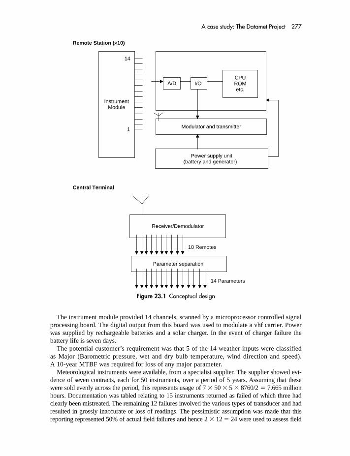
A case study: The Datamet Project 277
The instrument module provided 14 channels, scanned by a microprocessor controlled signalprocessing board. The digital output from this board was used to modulate a vhf carrier. Powerwas supplied by rechargeable batteries and a solar charger. In the event of charger failure thebattery life is seven days.
The potential customer’s requirement was that 5 of the 14 weather inputs were classifiedas Major (Barometric pressure, wet and dry bulb temperature, wind direction and speed).A 10-year MTBF was required for loss of any major parameter.
Meteorological instruments were available, from a specialist supplier. The supplier showed evi-dence of seven contracts, each for 50 instruments, over a period of 5 years. Assuming that thesewere sold evenly across the period, this represents usage of 7 � 50 � 5 � 8760/2 � 7.665 millionhours. Documentation was tabled relating to 15 instruments returned as failed of which three hadclearly been mistreated. The remaining 12 failures involved the various types of transducer and hadresulted in grossly inaccurate or loss of readings. The pessimistic assumption was made that thisreporting represented 50% of actual field failures and hence 2 � 12 � 24 were used to assess field
Remote Station (×10)
Central Terminal
14
InstrumentModule
A/D I/OCPUROMetc.
Modulator and transmitter
Power supply unit(battery and generator)
Receiver/Demodulator
Parameter separation
10 Remotes
14 Parameters
1
Figure 23.1 Conceptual design
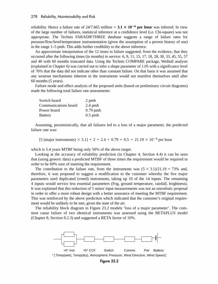
278 Reliability, Maintainability and Risk
reliability. Hence a failure rate of 24/7.665 million � 3.1 � 10�6 per hour was inferred. In viewof the large number of failures, statistical inference at a confidence level (i.e. Chi-square) was notappropriate. The Technis FARADIP.THREE database suggests a range of failure rates forpressure/flow/level/temperature instrumentation (given the assumption of a proven history of use)in the range 1–5 pmh. This adds further credibility to the above inference.
An approximate interpretation of the 12 times to failure suggested, from the evidence, that theyoccurred after the following times (in months) in service: 6, 9, 11, 15, 17, 18, 28, 30, 33, 45, 55, 57and 40 with 60 months truncated data. Using the Technis COMPARE package, Weibull analysis(explained in Chapter 6) was carried out to infer a shape parameter of 1.05 with a significance levelof 76% that the data did not indicate other than constant failure. On that basis it was assumed thatany wearout mechanisms inherent in the instruments would not manifest themselves until after60 months (5 years).
Failure mode and effect analysis of the proposed units (based on preliminary circuit diagrams)made the following total failure rate assessments:
Switch board 2 pmhCommunications board 2.4 pmhPower board 0.79 pmhBattery 0.5 pmh
Assuming, pessimistically, that all failures led to a loss of a major parameter, the predictedfailure rate was:
[5 (major instruments) � 3.1] � 2 � 2.4 � 0.79 � 0.5 � 21.19 � 10�6 per hour
which is 5.4 years MTBF being only 50% of the above target.Looking at the accuracy of reliability prediction (in Chapter 4, Section 4.4) it can be seen
that (using generic data) a predicted MTBF of three times the requirement would be required inorder to be 60% sure of meeting the requirement.
The contribution to the failure rate, from the instruments was (5 � 3.1)/21.19 � 73% and,therefore, it was proposed to suggest a modification to the customer whereby the five majorparameters used duplicated (voted) instruments, taking up 10 of the 14 inputs. The remaining4 inputs would service less essential parameters (Fog, ground temperature, rainfall, brightness).It was explained that this reduction of 5 minor input measurements was not an unrealistic proposalin order to offer a more robust design with a better assurance of meeting the MTBF requirement.This was reinforced by the above prediction which indicated that the customer’s original require-ment would be unlikely to be met, given the state of the art.
The reliability block diagram in Figure 23.2 models ‘loss of a major parameter’. The com-mon cause failure of two identical instruments was assessed using the BETAPLUS model(Chapter 8, Section 8.2.3) and suggested a BETA factor of 10%.
* [ Temp(wet), Temp(dry), Atmospheric Pressure, Wind Direction, Wind Speed ]
×5* Inst ×5* CCF Switch Comms Pwr Battery
Figure 23.2

A case study: The Datamet Project 279
Assuming a 6 month (4000 hour) proof-test interval then quantifying the model provides:
5 � (3.1 � 10�6)2 4000 � 5 � 10% � 3.1 � 10�6 � 2 � 10�6 � 2.4 � 10�6
� 0.79 � 10�6 � 0.5 � 10�6 � 7.43 � 10�6 per hour
which is an MTBF of 15 yearsAlthough only 1.5 times better than the requirement, since a conservative approach had been
taken in the failure rate assessment, it was decided to proceed with the design.
23.3 THE CONTRACT
The customer stated an intention to place a contract for the 10 systems and tabled a requirementsspecification together with the draft contract terms shown in Table 23.1.
The contract was signed and detailed development commenced. A 40-Year MTBF commitmentwas placed on the instrument supplier. The cost of a penalty repair visit was estimated to be £2000.
Table 23.1
(a) Ten years MTBF is required for loss of any major weather parameter (of which there will be fiveparameters) from each remote station. The supplier will satisfy the customer, by means of a reliabilityprediction, that the design is capable of meeting this requirement.
(b) The equipment must be capable of operating in a temperature range of 0–50 °C with a maximumrelative humidity of 80%.
(c) Failure shall consist of the loss of a major parameter or its incorrect measurement.
(d) For two year’s operation of the equipment, the contractor will refund the cost of all replacements tothe equipment. When a corrective maintenance visit, other than its coinciding with a schedule preventivemaintenance visit, is required the contractor will refund all labour and travelling costs including overtimeand incentives at a rate to be agreed.
(e) In the event of a system failure, the maximum repair time to restore the terminal to effective oper-ation shall be one hour. The contractor is required to show that the design is compatible with thistarget.
(f) In the event of systematic failures, the contractor shall perform all necessary design work andmake the necessary modifications to the system.
(g) The contractor is to use components having the most reasonable chance of being availablethroughout the life of the equipment and is required to state shelf life and number of spares to becarried in the case of any components that might cease to be available.
(h) The use of interchangeable printed cards may be employed and a positive means of identifyingwhich card is faulty must be provided so that, when the fault occurs, it can be rectified with the minimumeffort and skill. The insertion of cards in the wrong position shall be impossible or shall not causedamage to the cards or system.
(i) Maintenance instructions will be provided by the contractor and shall contain all necessaryinformation for the checking and maintenance of the system. These shall be comprehensive andgive full operational and functional information. The practice of merely providing a point-to-pointcomponent description of the circuits will not, in itself, be adequate.

280 Reliability, Maintainability and Risk
23.4 DETAILED DESIGN
Later in the detailed design phase, a more detailed failure mode and effect analysis was carriedout for the specific failure mode, ‘loss of a major parameter’. It produced a predicted MTBF of19 years which provided additional confidence in the design.
At the beginning of the integration test phase a failure reporting form was devised for recordingboth test and field failures. The customer was approached to the effect that, in view of the penaltyclause, full maintenance reporting documentation would be required to accompany all field claims.
It was noticed, during functional test, that a number of failures were due to timing and com-ponent tolerance problems rather than to catastrophic component failure.
Late in the development phase the instrument supplier went into liquidation and only 60 ofthe 100 sets of instruments, necessary for the initial project, could be supplied. Another wasfound but at 20% greater cost.
23.5 SYNDICATE STUDY
First session
Comment on the development and identify key areas of risk.
Second session
1. Discuss the contract clauses and construct alternatives either as:(i) The Producer(ii) The Customer
2. Set up a role-playing negotiation.
23.6 HINTS
Project
Having regard to the project size, as a percentage of turnover, decide if the project risk issueswere adequately addressed.
� Where is the most likely area of risk?� Were any activities omitted?� Should this have been undertaken as a development contract with separate production con-
tracts to follow?� Is MTBF the appropriate parameter for describing the performance (would not the customer
have responded to the suggestion of an Availability target?).� The single source of instruments (a critical component) was not wise. The field reliability
data did not apply to the second supplier thus reducing the value of the prediction.� What meaning had the 40-year MTBF requirement (on its own) in respect of instrument
procurement?� The drift-related failures, observed during development, were in addition to the random hard-
ware failures assumed in the FMEA model.� The 2nd FMEA offered a 20% improvement – was this significant?

A case study: The Datamet Project 281
Contract
(a) Appropriate parameters?(b) Is the description of the environment (in the contract) realistic? Rate of change is more
important than absolute values.(c) ‘Incorrect’ parameter? (See Chapter 19, Section 19.6)
(d1) When does the ‘two years’ start?(d2) If the MTBF target is met, what would the penalty visits represent as a percentage of the
contract price? What is the risk that the MTBF will be half of that target?(e) Maximum repair time! Can this be stipulated?(f) What criteria will allow a failure to be called systematic?

24 A case study: Gas DetectionSystem
This chapter is a case study, based on a typical gas detection system. It provides an example of thesafety-integrity targeting described in Chapter 22. The topic is fully covered in – Functional Safety:A Straightforward Guide to IEC 61508, 2nd edition, 2004, Smith D. J. and Simpson K. G. L.,Butterworth-Heinemann, ISBN 07506 6269 7.
Assume that our Gas Detection System has the primary function of providing an executiveaction input to some other ‘Emergency Shutdown’ system in order to protect a chemical processplant. This ESD system will close valves in order to isolate the flammable gases so as to pre-vent subsequent explosion or fire. It is assumed that successful operation of the Gas Detectionand ESD systems will prevent fatality.
24.1 SAFETY-INTEGRITY TARGET
In order to establish a safety-integrity target, it is necessary to establish a maximum tolerablefailure rate (or probability of failure on demand) for the safety-related system in question. Thetable of SIL targets (from IEC 61508) was shown and explained in Chapter 22.
If a maximum tolerable failure rate is to be established then, in turn, a maximum tolerablerisk of fatality must first be stated. There are no hard and fast rules but a typical guide, from theInstitution of Gas Engineers and Managers Recommendations SR/15, suggests:
Scenario Maximum Individual Risk of Fatality
VOLUNTARY (EMPLOYEE) 10�4 paINVOLUNTARY (PUBLIC) 10�5 pa
It might be argued that the operatives in this plant are accepting a voluntary risk and that the10�4 per annum should apply. It might also be argued that there is approximately an order of mag-nitude of plant-related hazards that could lead to fatality and, thus, the maximum tolerable risk inrespect of this Gas Detection-related hazard should be an order less, namely 10�5 per annum.
For the particular application, the following judgements were made:
Person(s) at risk (16 hours per day) 67%Probability of gas release finding a source of ignition 80%Probability that subsequent fire/explosion leads to fatality 50%

A case study: Gas Detection System 283
It follows that the maximum tolerable failure rate for this event (given the above maximumtolerable risk) is:
10�5 pa/(0.67 � 0.8 � 0.5) � 3.7 � 10�5 pa
Further, assume that a fault tree has been constructed to model all the causes of a suitablylarge gas release which places a demand on this system of mitigation, and that it predicts ademand of 1.5 � 10�3 per annum.
It follows that the maximum tolerable probability of failure on demand for the mitigation is:
3.7 � 10�5 pa/1.5 � 10�3 pa � 2.5 � 10�2
Since neither the Gas Detection nor the ESD systems must fail then this target has to beshared between them. Assume that, for other reasons, the probability of failure on demand tar-get for the ESD system has been established as 5 � 10�3.
It follows that our Gas Detection System attracts a maximum tolerable probability offailure on demand (PFD) target of 2.5 � 10�2 � 5 � 10�3 � 2 � 10�2 which imposes aSIL 1 target (see Chapter 22, Table 22.1)
24.2 RANDOM HARDWARE FAILURES
One of the five things that IEC 61508 requires to be demonstrated in respect of the SIL target(Chapter 22) is that the hardware reliability meets the target failure rate or PFD for the haz-ardous failure mode in question. In this case we are required to show a PFD of 2 � 10�2 orbetter for the failure mode ‘fail to detect or respond to a valid gas concentration’.
Each area is served by a group of three pellister hydrocarbon gas detectors each of which isassumed to be able to sense any given release. Any one detector sensing gas will give rise to analarm. This, with operator response, may well be sufficient to mitigate the hazards. However,the safety function addressed here is as follows. Any two out of three detectors sensing gas willgive rise to an executive output which is the signal to the ESD. It is this latter function which isthe SIL 1 targetted safety-function in question.
A simplified but realistic reliability block diagram of the Gas Detection System is shown inFigure 24.1. Each group of three detectors is spread over three separate input PLC cards in orderto maximize the redundancy. The executive action is provided by a single (unvoted) output card
Detector 1
Detector 2
Detector 3
I/P card 1
I/P card 2
O/P card
I/P card 3
CommonCauseFailure
ProcessorUndiagnosed
ProcessorDiagnosed
Figure 24.1 Reliability block diagram

284 Reliability, Maintainability and Risk
with a normally de-energized relay operating to open a closed contact which provides an inputsignal to the ESD system. The failure data used for the prediction (taken from the TECHNISFARADIP.THREE data bank) are:
Pellister gas detector fail to respond 5 � 10�6 per hrPLC input card fail to respond 0.05 � 10�6 per hrPLC processor card fail to output 0.05 � 10�6 per hrPLC output card fail to release relay 0.05 � 10�6 per hrRelay coil fail to energize 0.05 � 10�6 per hrRelay contact contact s/c 0.045 � 10�6 per hr
Assume that 90% of the dormant failures, in the processor module, are diagnosed by auto-test and are corrected in one week. Assume, also, that the remainder are revealed by proof testand that the proof-test interval is 8000 hours (i.e. c. 12 months).
A common cause BETA factor of 10% is assumed. The block diagram is quantified using themathematics from Chapters 8 and 9. The probability of failure on demand is:
(a) Triplicated detector/input card (2 out of 3)
�2 T 2 (from Table 8.4) � (5 � 10�6 � 0.05 � 10�6)2 � 80002 � 1.6 � 10�3
(b) Common cause failure
10% � T/2 � 10% � (5 � 10�6 � 0.05 � 10�6) � 4000 � 2 � 10�3
(c) ProcessorDiagnosed (by auto-test) failures:
90% � MDT � 90% � (0.05 � 10�6) � 168 � 7.6 � 10�6
Undiagnosed (by auto-test) failures:
10% � T/2 � 10% � 0.05 � 10�6 � 4000 � 2 � 10�5
(d) Output card
� T/2 � 0.05 � 10�6 � 4000 � 2 � 10�4
(e) Relay coil fails to operate
� T/2 � 0.05 � 10�6 � 4000 � 2 � 10�4
(f) Relay contact fails to open
� T/2 � 0.045 � 10�6 � 4000 � 1.8 � 10�4
Total � 4.2 � 10�3
Which meets the target of 2 � 10�2 by nearly an order of magnitude.

A case study: Gas Detection System 285
24.3 ALARP
The Standard (IEC 61508) requires us to address ALARP (As low as is reasonably practicable)which was dealt with in Chapters 3 and 10. In this case we will assume a cost per life saved cri-teria of £2 000 000. If the Broadly Acceptable Risk is taken as 10�6 pa, then by the same tokenas above we will reduce this by ten to 10�7 pa for this hazard.
Now, if the maximum tolerable PFD of 2 � 10�2 corresponds to a risk of 10�5 pa, then the4.2 � 10�3 (predicted) corresponds to a risk of 10�5 pa � 4.2 � 10�3/2 � 10�2 � 2.1 � 10�6 pa.This is greater than the Broadly Acceptable Risk and we argue as follows.
Any proposal which would reduce the risk further (to the Broadly Acceptable Level) can betested, given a two fatality scenario and a 25-year plant life, by:
£2 000 000 � (Max cost of proposal)/[(2.1 � 10�6 � 1 � 10�7) � 2 fatalities � 25 years]
Therefore Max cost of proposal � £200.Since it is unlikely that any further risk reduction can be achieved within this sum, ALARP
might be argued to have been satisfied.
24.4 ARCHITECTURES
In Chapter 22 a brief explanation of the Safe Failure Fraction was given. This is more fullycovered in Functional Safety: A Straightforward Guide to IEC 61508.
In this case study the SIL 1 target imposes safe failure fraction targets as follows:
The single PLC being a Type B deviceGreater than 60%. It is very likely that this could be demonstrated.
The voted pellister gas detector assuming it can be treated as a Type A deviceNo special requirement.
24.5 LIFE-CYCLE ACTIVITIES
It will be necessary to demonstrate that certain life-cycle activities have been carried out. Thisis addressed in detail in Functional Safety: A Straightforward Guide to IEC 61508.
24.6 FUNCTIONAL SAFETY CAPABILITY
It is also necessary to demonstrate, not only that the life-cycle activities have been carried out,but that the company’s management system ensures that they will always be carried out. Thisinvolves competencies and quality management procedures and is dealt with in FunctionalSafety: A Straightforward Guide to IEC 61508.
Appendix 1 Glossary
A1 TERMS RELATED TO FAILURE
A1.1 Failure
Termination of the ability of an item to perform Meaningless without its specified function. OR, Non-conformance to performance specsome defined performance criteria. Failures maybe classified by:
1. Cause – Chapter 2Misuse: Caused by operation outside specified stress.Primary: Not caused by an earlier failure.Secondary: Caused by an earlier failure.Wearout: Caused by accelerating failure rate mechanism.Design: Caused by an intrinsic weakness.
Software: Caused by a program error despite Chapter 17no hardware failure
2. Type –Sudden: Not anticipated and no prior degradation.Degradation: Parametric drift or gradual reduction in performance.Intermittent: Alternating between the failed and operating condition.Dormant: A component or unit failure which does not cause system failure but which eitherhastens it or, in combination with another dormant fault, would cause system failure.Random: Failure is equally probable in eachsuccessive equal time interval.Catastrophic: Sudden and complete.
A1.2 Failure mode
The outward appearance of a specific failure Chapter 2effect (e.g. open circuit, leak to atmosphere).

Appendix 1 287
A1.3 Failure mechanism
The physical or chemical process which causes Chapter 11the failure.
A1.4 Failure rate
The number of failures of an item per unit time. Per hour, cycle,operation, etc.
This can be applied to:
1. Observed failure rate: as computed from a sample. Point estimate2. Assessed failure rate: as inferred from sample Involves a confidence
information. level3. Extrapolated failure rate: projected to other
stress levels.
A1.5 Mean Time Between Failures and Mean Time to Fail
The total cumulative functioning time of a populationdivided by the number of failures. As with failure rate,the same applies to Observed, Assessed and ExtrapolatedMTBF. MTBF is used for items which involve repair.MTTF is used for items with no repair.
A1.6 Common Cause Failure
The result of an event(s) which, because of Section 8.2dependencies, causes a coincidence of failurestates of components in two or more separatechannels of a redundant system, leading to thedefined system failing to perform its intended function.
A1.7 Common Mode Failure
A subset of Common Cause Failure whereby Section 8.2two or more components fail in the same manner.
A2 RELIABILITY TERMS
A2.1 Reliability
The probability that an item will perform a required function, under stated conditions, for astated period of time.
Since observed reliability is empirical it is defined as the ratio of items which perform their function for the stated period to the total number in the sample.

288 Reliability, Maintainability and Risk
A2.2 Redundancy
The provision of more than one means of achievinga function.
Active: All items remain operating prior to failure.Standby: Replicated items do not operate untilneeded.
A2.3 Diversity
The same performance of a function by two or more Chapter 17independent and dissimilar means (of particularrelevance to software).
A2.4 Failure mode and effect analysis
Determining the outcomes of all known failure modes Section 9.3within an assembly or circuit.
A2.5 Fault tree analysis
A graphical method of modelling a system failure Section 8.3using AND and OR logic in tree form.
A2.6 Cause consequence analysis (Event trees)
A graphical method of modelling one or more Section 8.4outcomes of a failure or of an event by means of interconnected YES/NO decision boxes.
A2.7 Reliability growth
Increase in reliability as a result of continued Section 12.3design modifications resulting from field datafeedback.
A2.8 Reliability centred maintenance
The application of quantified reliability techniques Chapter 16to optimizing discard, times, proof-test intervalsand spares levels.
A3 MAINTAINABILITY TERMS
A3.1 Maintainability
The probability that a failed item will be restored to operational effectiveness within a given period of time when the repair action is performed in accordance with prescribed procedures.

Appendix 1 289
A3.2 Mean Time to Repair (MTTR)
The mean time to carry out a defined maintenance Usually refers toaction. corrective maintenance
A3.3 Repair rate
The reciprocal of MTTR. When used in reliability calculations it is thereciprocal of Down Time
A3.4 Repair time
The time during which an item is undergoing Must be carefully Chapter 14diagnosis, repair, checkout and alignment. defined; may also and Section
depend on diagnostics 9.2
A3.5 Down time
The time during which an item is not able to Must be carefully definedperform to specification.
A3.6 Corrective maintenance
The actions associated with repair time.
A3.7 Preventive maintenance
The actions, other than corrective maintenance,carried out for the purpose of keeping an item in a specified condition.
A3.8 Least Replaceable Assembly (LRA)
That assembly at which diagnosis ceases and Typically a printed-boardreplacement is carried out. assembly
A3.9 Second-line maintenance
Maintenance of LRAs which have been removedfrom the field for repair or for preventive maintenance.
A4 TERMS ASSOCIATED WITH SOFTWARE
A4.1 Software
All documentation and inputs (for example, Chapter 17tapes, disks) associated with programmable devices.
A4.2 Programmable device
Any piece of equipment containing one or morecomponents which provides a computer architecturewith memory facilities.

290 Reliability, Maintainability and Risk
A4.3 High-level language
A means of writing program instructions usingsymbols each of which represents severalprogram steps.
A4.4 Assembler
A program for converting program instructions,written in mnemonics, into binary machine codesuitable to operate a programmable device.
A4.5 Compiler
A program which, in addition to being an assembler,generates more than one instruction for each statementthereby permitting the use of a high-level language.
A4.6 Diagnostic software
A program containing self-test algorithms enabling Particularly applicablefailures to be identified. to ATE
A4.7 Simulation
The process of representing a unit or system bysome means in order to provide some or allidentical inputs, at some interface, for testpurposes. A means of prediction.
A4.8 Emulation
A type of simulation whereby the simulator Identical to the realresponds to all possible inputs as would the item from the point ofreal item and generates all the corresponding view of a unit under testoutputs.
A4.9 Load test
A system test involving simulated inputs in orderto prove that the system will function atfull load.
A4.10 Functional test
An empirical test routine designed to exercise anitem such that all aspects of the software arebrought into use.
A4.11 Software error
An error in the digital state of a system whichmay propagate to become a failure.

Appendix 1 291
A4.12 Bit error rate
The random incidence of incorrect binary digits. Expressed 10�x/bit
A4.13 Automatic Test Equipment (ATE)
Equipment for stimulus and measurement controlledby a programmed sequence of steps(usually in software).
A4.14 Data corruption
The introduction of an error by reason of somechange to the software already resident in thesystem. This could arise from electrical interferenceor from incorrect processing of a portion of the software.
A5 TERMS RELATED TO SAFETY
A5.1 Hazard
A scenario whereby there is a potential forhuman, property or environmental damage.
A5.2 Major hazard
A general, imprecise, term for large-scale hazardsas, for example, in the chemical or nuclear industries.
A5.3 Hazard Analysis
A term which refers to a number of techniques Chapter 10for analysing the events leading to a hazardous situation.
A5.4 HAZOP
Hazard and Operability Study – a formal analysis Chapter 10of a process or plant by the application of guidewords.
A5.5 Risk
The likelihood, expressed either as a probability Chapters 3or as a frequency, of a hazard materializing. and 10
A5.6 Consequence analysis
Techniques which involve quantifying the outcomeof failures in terms of dispersion, radiation, fatality, etc.
A5.7 Safe Failure Fraction
The proportion of failures which are either near-hazardous Chapter 22or are detected hazardous failures.

292 Reliability, Maintainability and Risk
A5.8 Safety-integrity
The probability of a system performing specificsafety functions in a stated period of time.
A5.9 Safety-integrity level
One of 4 discrete target levels for specifyingsafety-integrity requirements.
A6 MISCELLANEOUS TERMS
A6.1 Availability (steady state)
The proportion of time that an item is capable of Given as:operating to specification within a large time MTBF/(MTBF � MDT)interval.
A6.2 Unavailability (PFD)
The proportion of time that an item is NOTcapable of operating to specification withina large time interval. Since the probability offailure on demand (PFD) is the probability ofthe item not being ‘available’, then PFD is thesame as unavailability.
A6.3 Burn-in
The operation of items for a specified period oftime in order to remove early failures and bringthe reliability characteristic into the random failurepart of the Bathtub Curve.
A6.4 Confidence interval
A range of a given variable within which a random Chapter 5value will lie at a stated confidence(probability).
A6.5 Consumer’s risk
The probability of an unacceptable batch beingaccepted owing to a favourable sample.
A6.6 Derating
The use of components having a higher strengthrating in order to reduce failure rate.

Appendix 1 293
A6.7 Ergonomics
The study of human/machine interfaces in order tominimize human errors due to mental orphysical fatigue.
A6.8 Mean
Usually used to indicate the Arithmetic Mean, whichis the sum of a number of values divided by thenumber thereof.
A6.9 Median
The median is that value such that 50% of thevalues in question are greater and 50% less than it.
A6.10 Producer’s risk
The probability of an acceptable batch beingrejected owing to an unfavourable sample.
A6.11 Quality
Conformance to specification.
A6.12 Random
Such that each item has the same probability ofbeing selected as any other.
A6.13 FRACAS
An acronym meaning failure reporting andcorrective action system.
A6.14 RAMS
A general term for reliability, availability,maintainability and safety-integrity.

Appendix 2 Percentage points of theChi-square distribution
0.9995 0.999 0.995 0.990 0.975 0.95 0.90 0.80 0.70 0.60
1 0.06393 0.05157 0.04393 0.03157 0.03982 0.02393 0.0158 0.0642 0.148 0.2752 0.02100 0.02200 0.0100 0.0201 0.0506 0.103 0.211 0.446 0.713 1.023 0.0153 0.0243 0.0717 0.115 0.216 0.352 0.584 1.00 1.42 1.874 0.0639 0.0908 0.207 0.297 0.484 0.711 1.06 1.65 2.19 2.755 0.158 0.210 0.412 0.554 0.831 1.15 1.61 2.34 3.00 3.66
6 0.299 0.381 0.676 0.872 1.24 1.64 2.20 3.07 3.83 4.577 0.485 0.598 0.989 1.24 1.69 2.17 2.83 3.82 4.67 5.498 0.710 0.857 1.34 1.65 2.18 2.73 3.49 4.59 5.53 6.429 0.972 1.15 1.73 2.09 2.70 3.33 4.17 5.38 6.39 7.36
10 1.26 1.48 2.16 2.56 3.25 3.94 4.87 6.18 7.27 8.30
11 1.59 1.83 2.60 3.05 3.82 4.57 5.58 6.99 8.15 9.2412 1.93 2.21 3.07 3.57 4.40 5.23 6.30 7.81 9.03 10.213 2.31 2.62 3.57 4.11 5.01 5.89 7.04 8.63 9.93 11.114 2.70 3.04 4.07 4.66 5.63 6.57 7.79 9.47 10.8 12.115 3.11 3.48 4.60 5.23 6.26 7.26 8.55 10.3 11.7 13.0
16 3.54 3.94 5.14 5.81 6.91 7.96 9.31 11.2 12.6 14.017 3.98 4.42 5.70 6.41 7.56 8.67 10.1 12.0 13.5 14.918 4.44 4.90 6.26 7.01 8.23 9.39 10.9 12.9 14.4 15.919 4.91 5.41 6.84 7.63 8.91 10.0 11.7 13.7 15.4 16.920 5.40 5.92 7.43 8.26 9.59 10.9 12.4 14.6 16.3 17.8
21 5.90 6.45 8.03 8.90 10.3 11.6 13.2 15.4 17.2 18.822 6.40 6.98 8.64 9.54 11.0 12.3 14.0 16.3 18.1 19.723 6.92 7.53 9.26 10.2 11.7 13.1 14.8 17.2 19.0 20.724 7.45 8.08 9.98 10.9 12.4 13.8 15.7 18.1 19.9 21.725 7.99 8.65 10.5 11.5 13.1 14.6 16.5 18.9 20.9 22.6
26 8.54 9.22 11.2 12.2 13.8 15.4 17.3 19.8 21.8 23.627 9.09 9.80 11.8 12.9 14.6 16.2 18.1 20.7 22.7 24.528 9.66 10.4 12.5 13.6 15.3 16.9 18.9 21.6 23.6 25.529 10.2 11.0 13.1 14.3 16.0 17.7 19.8 22.5 24.6 26.530 10.8 11.6 13.8 15.0 16.8 18.5 20.6 23.4 25.5 27.4
31 11.4 12.2 14.5 15.7 17.5 19.3 21.4 24.3 26.4 28.432 12.0 12.8 15.1 16.4 18.3 20.1 22.3 25.1 27.4 29.433 12.6 13.4 15.8 17.1 19.0 20.9 23.1 26.0 28.3 30.334 13.2 14.1 16.5 17.8 19.8 21.7 24.0 26.9 29.2 31.335 13.8 14.7 17.2 18.5 20.6 22.5 24.8 27.8 30.2 32.3
36 14.4 15.3 17.9 19.2 21.3 23.3 25.6 28.7 31.1 33.337 15.0 16.0 18.6 20.0 22.1 24.1 26.5 29.6 32.1 34.238 15.6 16.6 19.3 20.7 22.9 24.9 27.3 30.5 33.0 35.239 16.3 17.3 20.0 21.4 23.7 25.7 28.2 31.4 33.9 36.240 16.9 17.9 20.7 22.2 24.4 26.5 29.1 32.3 34.9 37.1
41 17.5 18.6 21.4 22.9 25.2 27.3 29.9 33.3 35.8 38.142 18.2 19.2 22.1 23.7 26.0 28.1 30.8 34.2 36.8 39.143 18.8 19.9 22.9 24.4 26.8 29.0 31.6 35.1 37.7 40.044 19.5 20.6 23.6 25.1 27.6 29.8 32.5 36.0 38.6 41.045 20.1 21.3 24.3 25.9 28.4 30.6 33.4 36.9 39.6 42.0
46 20.8 21.9 25.0 26.7 29.1 31.4 34.2 37.8 40.5 43.047 21.5 22.6 25.8 27.4 30.0 32.3 35.1 38.7 41.5 43.948 22.1 23.3 26.5 28.2 30.8 33.1 35.9 39.6 42.4 44.949 22.8 24.0 27.2 28.9 31.6 33.9 36.8 40.5 43.4 45.950 23.5 24.7 28.0 29.7 32.4 34.8 37.7 41.4 44.3 46.9
�
n

Appendix 2 295
0.50 0.40 0.30 0.20 0.10 0.05 0.025 0.01 0.005 0.001 0.0005
0.455 0.708 1.07 1.64 2.71 3.84 5.02 6.63 7.88 10.8 12.1 11.39 1.83 2.41 3.22 4.61 5.99 7.38 9.21 10.6 13.8 15.2 22.37 2.95 3.67 4.64 6.25 7.81 9.35 11.3 12.8 16.3 17.7 33.36 4.04 4.88 5.99 7.78 9.49 11.1 13.3 14.9 18.5 20.0 44.35 5.13 6.06 7.29 9.24 11.1 12.8 15.1 16.7 20.5 22.1 5
5.35 6.21 7.23 8.56 10.6 12.6 14.4 16.8 18.5 22.5 24.1 66.35 7.28 8.38 9.80 12.0 14.1 16.0 18.5 20.3 24.3 26.0 77.34 8.35 9.52 11.0 13.4 15.5 17.5 20.1 22.0 26.1 27.9 88.34 9.41 10.7 12.2 14.7 16.9 19.0 21.7 23.6 27.9 29.7 99.34 10.5 11.8 13.4 16.0 18.3 20.5 23.2 25.2 29.6 31.4 10
10.3 11.5 12.9 14.6 17.3 19.7 21.9 24.7 26.8 31.3 33.1 1111.3 12.6 14.0 15.8 18.5 21.0 23.3 26.2 28.3 32.9 34.8 1212.3 13.6 15.1 17.0 19.8 22.4 24.7 27.7 29.8 34.5 36.5 1313.3 14.7 16.2 18.2 21.1 23.7 26.1 29.1 31.3 36.1 38.1 1414.3 15.7 17.3 19.3 22.3 25.0 27.5 30.6 32.8 37.7 39.7 15
15.3 16.8 18.4 20.5 23.5 26.3 28.8 32.0 34.3 39.3 41.3 1616.3 17.8 19.5 21.6 24.8 27.6 30.2 33.4 35.7 40.8 42.9 1717.3 18.9 20.6 22.8 26.0 28.9 31.5 34.8 37.2 42.3 44.4 1818.3 19.9 21.7 23.9 27.2 30.1 32.9 36.2 38.6 43.8 46.0 1919.3 21.0 22.8 25.0 28.4 31.4 34.2 37.6 40.0 45.3 47.5 20
20.3 22.0 23.9 26.2 29.6 32.7 35.5 38.9 41.4 46.8 49.0 2121.3 23.0 24.9 27.3 30.8 33.9 36.8 40.3 42.8 48.3 50.5 2222.3 24.1 26.0 28.4 32.0 35.2 38.1 41.6 44.2 49.7 52.0 2323.3 25.1 27.1 29.6 33.2 36.4 39.4 43.0 45.6 51.2 53.5 2424.3 26.1 28.2 30.7 34.4 37.7 40.6 44.3 46.9 52.6 54.9 25
25.3 27.2 29.2 31.8 35.6 38.9 41.9 45.6 48.3 54.1 56.4 2626.3 28.2 30.3 32.9 36.7 40.1 43.2 47.0 49.6 55.5 57.9 2727.3 29.2 31.4 34.0 37.9 41.3 44.5 48.3 51.0 56.9 59.3 2828.3 30.3 32.5 35.1 39.1 42.6 45.7 49.6 52.3 58.3 60.7 2929.3 31.3 33.5 36.3 40.3 43.8 47.0 50.9 53.7 59.7 62.2 30
30.3 32.3 34.6 37.4 41.4 45.0 48.2 52.2 55.0 61.1 63.6 3131.3 33.4 35.7 38.5 42.6 46.2 49.5 53.5 56.3 62.5 65.0 3232.2 34.4 36.7 39.6 43.7 47.4 50.7 54.8 57.6 63.9 66.4 3333.3 35.4 37.8 40.7 44.9 48.6 52.0 56.1 59.0 65.2 67.8 3434.3 36.5 38.9 41.8 46.1 49.8 53.2 57.3 60.3 66.6 69.2 35
35.3 37.5 39.9 42.9 47.2 51.0 54.4 58.6 61.6 68.0 70.6 3636.3 38.5 41.0 44.0 48.4 52.2 55.7 59.9 62.9 69.3 72.0 3737.3 39.6 42.0 45.1 49.5 53.4 56.9 61.2 64.2 70.7 73.4 3838.3 40.6 43.1 46.2 50.7 54.6 58.1 62.4 65.5 72.1 74.7 3939.3 41.6 44.2 47.3 51.8 55.8 59.3 63.7 66.8 73.4 76.1 40
40.3 42.7 45.2 48.4 52.9 56.9 60.6 65.0 68.1 74.7 77.5 4141.3 43.7 46.3 49.5 54.1 58.1 61.8 66.2 69.3 76.1 78.8 4242.3 44.7 47.3 50.5 55.2 59.3 63.0 67.5 70.6 77.4 80.2 4343.3 45.7 48.4 51.6 56.4 60.5 64.2 68.7 71.9 78.7 81.5 4444.3 46.8 49.5 52.7 57.5 61.7 65.4 70.0 73.2 80.1 82.9 45
45.3 47.8 50.5 53.8 58.6 62.8 66.6 71.2 74.4 81.4 84.2 4646.3 48.8 51.6 54.9 59.8 64.0 67.8 72.4 75.7 82.7 85.6 4747.3 49.8 52.6 56.0 60.9 65.2 69.0 73.7 77.0 84.0 86.9 4848.3 50.9 53.7 57.1 62.0 66.3 70.2 74.9 78.2 85.4 88.2 4949.3 51.9 54.7 58.2 63.2 67.5 71.4 76.2 79.5 86.7 89.6 50
�
n

296 Reliability, Maintainability and Risk
0.9995 0.999 0.995 0.990 0.975 0.95 0.90 0.80 0.70 0.60 0.50
51 24.1 25.4 28.7 30.5 33.2 35.6 38.6 42.4 45.3 47.8 50.352 24.8 26.1 29.5 31.2 34.0 36.4 39.4 43.3 46.2 48.8 51.353 25.5 26.8 30.2 32.0 34.8 37.3 40.3 44.2 47.2 49.8 52.354 26.2 27.5 31.0 32.8 35.6 38.1 41.2 45.1 48.1 50.8 53.355 26.9 28.2 31.7 33.6 36.4 39.0 42.1 46.0 49.1 51.7 54.3
56 27.6 28.9 32.5 34.3 37.2 39.8 42.9 47.0 50.0 52.7 55.357 28.2 29.6 33.2 35.1 38.0 40.6 43.8 47.9 51.0 53.7 56.358 28.9 30.3 34.0 35.9 38.8 41.5 44.7 48.8 51.9 54.7 57.359 29.6 31.0 34.8 36.7 39.7 42.3 45.6 49.7 52.9 55.6 58.360 30.3 31.7 35.5 37.5 40.5 43.2 46.5 50.6 53.8 56.6 59.3
61 31.0 32.5 36.3 38.3 41.3 44.0 47.3 51.6 54.8 57.6 60.362 31.7 33.2 37.1 39.1 42.1 44.9 48.2 52.5 55.7 58.6 61.363 32.5 33.9 37.8 39.9 43.0 45.7 49.1 53.5 56.7 59.6 62.364 33.2 34.6 38.6 40.6 43.8 46.6 50.0 54.3 57.6 60.5 63.365 33.9 35.4 39.4 41.4 44.6 47.4 50.9 55.3 58.6 61.5 64.3
66 34.6 36.1 40.2 42.2 45.4 48.3 51.8 56.2 59.5 62.5 65.367 35.3 36.8 40.9 43.0 46.3 49.2 52.7 57.1 60.5 63.5 66.368 36.0 37.6 41.7 43.8 47.1 50.0 53.5 58.0 61.4 64.4 67.369 36.7 38.3 42.5 44.6 47.9 50.9 54.4 59.0 62.4 65.4 68.370 37.5 39.0 43.3 54.4 48.8 51.7 55.3 59.9 63.3 66.4 69.3
71 38.2 39.8 44.1 46.2 49.6 52.6 56.2 60.8 64.3 67.4 70.372 38.9 40.5 44.8 47.1 50.4 53.5 57.1 61.8 65.3 68.4 71.373 39.6 41.3 45.6 47.9 51.3 54.3 58.0 62.7 66.2 69.3 72.374 40.4 42.0 40.4 48.7 52.1 55.2 58.9 63.6 67.2 70.3 73.375 41.1 42.8 47.2 49.5 52.9 56.1 59.8 64.5 68.1 71.3 74.3
76 41.8 43.5 48.0 50.3 53.8 56.9 60.7 65.5 69.1 72.3 75.377 42.6 44.3 48.8 51.1 54.6 57.8 61.6 66.4 70.0 73.2 76.378 43.3 45.0 49.6 51.9 55.5 58.7 62.5 67.3 71.0 74.2 77.379 44.1 45.8 50.4 52.7 56.3 59.5 63.4 68.3 72.0 75.2 78.380 44.8 46.5 51.2 53.5 57.2 60.4 64.3 69.2 72.9 76.2 79.3
81 45.5 47.3 52.0 54.4 58.0 61.3 65.2 70.1 73.9 77.2 80.382 46.3 48.0 52.8 55.2 58.8 62.1 66.1 71.1 74.8 78.1 81.383 47.0 48.8 53.6 56.0 59.7 63.0 67.0 72.0 75.8 79.1 82.384 47.8 49.6 54.4 56.8 60.5 63.9 67.9 72.9 76.8 80.1 83.385 48.5 50.3 55.2 57.6 61.4 64.7 68.8 73.9 77.7 81.1 84.3
86 49.3 51.1 56.0 58.5 62.2 65.6 69.7 74.8 78.7 82.1 85.387 50.0 51.9 56.8 59.3 63.1 66.5 70.6 75.7 79.6 83.0 86.388 50.8 52.6 57.6 60.1 63.9 67.4 71.5 76.7 80.6 84.0 87.389 51.5 53.4 58.4 60.9 64.8 68.2 72.4 77.6 81.6 85.0 88.390 52.3 54.2 59.2 61.8 65.6 69.1 73.3 78.6 82.5 86.0 89.3
91 53.0 54.9 60.0 62.6 66.5 70.0 74.2 79.5 83.5 87.0 90.392 53.8 55.7 60.8 63.4 67.4 70.9 75.1 80.4 84.4 88.0 91.393 54.5 56.5 61.6 64.2 68.2 71.8 76.0 81.4 85.5 88.9 92.394 55.3 57.2 62.4 65.1 69.1 72.6 76.9 82.3 86.4 89.9 93.395 56.1 58.0 63.2 65.9 69.9 73.5 77.8 83.2 87.3 90.9 94.3
96 56.8 58.8 64.1 66.7 70.8 74.4 78.7 84.2 88.3 91.9 95.397 57.6 59.6 64.9 67.6 71.6 75.3 79.6 85.1 89.2 92.9 96.398 58.4 60.4 65.7 68.4 72.5 76.2 80.5 86.1 90.2 93.8 97.399 59.1 61.1 66.5 69.2 73.4 77.0 81.4 87.0 91.2 94.8 98.3
100 59.9 61.9 67.3 70.1 74.2 77.9 82.4 87.9 92.1 95.8 99.3
�
n

Appendix 2 297
0.40 0.30 0.20 0.10 0.05 0.025 0.01 0.005 0.001 0.0005
52.9 55.8 59.2 64.3 68.7 72.6 77.4 80.7 88.0 90.9 5153.9 56.8 60.3 65.4 69.8 73.8 78.6 82.0 89.3 92.2 5255.0 57.9 61.4 66.5 71.0 75.0 79.8 83.3 90.6 93.5 5356.0 58.9 62.5 67.7 72.2 76.2 81.1 84.5 91.9 94.8 5457.0 60.0 63.6 68.8 73.3 77.4 82.3 85.7 93.2 96.2 55
58.0 61.0 64.7 69.9 74.5 78.6 83.5 87.0 94.5 97.5 5659.1 62.1 65.7 71.0 75.6 79.8 84.7 88.2 95.8 98.8 5760.1 63.1 66.8 72.2 76.8 80.9 86.0 89.5 97.0 100.1 5861.1 64.2 67.9 73.3 77.9 82.1 87.2 90.7 98.3 101.4 5962.1 65.2 69.0 74.4 79.1 83.3 88.4 92.0 99.6 102.7 60
63.2 66.3 70.0 75.5 80.2 84.5 89.6 93.2 100.9 104.0 6164.2 67.3 71.1 76.6 81.4 85.7 90.8 94.4 102.2 105.3 6265.2 68.4 72.2 77.7 82.5 86.8 92.0 95.6 103.4 106.6 6366.2 69.4 73.3 78.9 83.7 88.0 93.2 96.9 104.7 107.9 6467.2 70.5 74.4 80.0 84.8 89.2 94.4 98.1 106.0 109.2 65
68.3 71.5 75.4 81.1 86.0 90.3 95.6 99.3 107.3 110.5 6669.3 72.6 76.5 82.2 87.1 91.5 96.8 100.6 108.5 111.7 6770.3 73.6 77.6 83.3 88.3 92.7 98.0 101.8 109.8 113.0 6871.3 74.6 78.6 84.4 89.4 93.9 99.2 103.0 111.1 114.3 6972.4 75.7 79.7 85.5 90.5 95.0 100.4 104.2 112.3 115.6 70
73.4 76.7 80.8 86.6 91.7 96.2 101.6 105.4 113.6 116.9 7174.4 77.8 81.9 87.7 92.8 97.4 102.8 106.6 114.8 118.1 7275.4 78.8 82.9 88.8 93.9 98.5 104.0 107.9 116.1 119.4 7376.4 79.9 84.0 90.0 95.1 99.7 105.2 109.1 117.3 120.7 7477.5 80.9 85.1 91.1 96.2 100.8 106.4 110.3 118.6 121.9 75
78.5 82.0 86.1 92.2 97.4 102.0 107.6 111.5 119.9 123.2 7679.5 83.0 87.2 93.3 98.5 103.2 108.8 112.7 121.1 124.5 7780.5 84.0 88.3 94.4 99.6 104.3 110.0 113.9 122.3 125.7 7881.5 85.1 89.3 95.5 100.7 105.5 111.1 115.1 123.6 127.0 7982.6 86.1 90.4 96.6 101.9 106.6 112.3 116.3 124.3 128.3 80
83.6 87.2 91.5 97.7 103.0 107.8 113.5 117.5 126.1 129.5 8184.6 88.2 92.5 98.8 104.1 108.9 114.7 118.7 127.3 130.8 8285.6 89.2 93.6 99.9 105.3 110.1 115.9 119.9 128.6 132.0 8386.6 90.3 94.7 101.0 106.4 111.2 117.1 121.1 129.8 133.3 8487.7 91.3 95.7 102.1 107.5 112.4 118.2 122.3 131.0 134.5 85
88.7 92.4 96.8 103.2 108.6 113.5 119.4 123.5 132.3 135.8 8689.7 93.4 97.9 104.3 109.8 114.7 120.6 124.7 133.5 137.0 8790.7 94.4 98.9 105.4 110.9 115.8 121.8 125.9 134.7 138.3 8891.7 95.5 100.0 106.5 112.0 117.0 122.9 127.1 136.0 139.5 8992.8 96.5 101.1 107.6 113.1 118.1 124.1 128.3 137.2 140.8 90
93.8 97.6 102.1 108.7 114.3 119.3 125.3 129.5 138.4 142.0 9194.8 98.6 103.2 109.8 115.4 120.4 126.5 130.7 139.7 143.3 9295.8 99.6 104.2 110.9 116.5 121.6 127.6 131.9 140.9 144.5 9396.8 100.7 105.3 111.9 117.6 122.7 128.8 133.1 142.1 145.8 9497.9 101.7 106.4 113.0 118.8 123.9 130.0 134.2 143.3 147.0 95
98.9 102.8 107.4 114.1 119.9 125.0 131.1 135.4 144.6 148.2 9699.9 103.8 108.5 115.2 121.0 126.1 132.3 136.6 145.8 149.5 97
100.9 104.8 109.5 116.3 122.1 127.3 133.5 137.8 147.0 150.7 98101.9 105.9 110.6 117.4 123.2 128.4 134.6 139.0 148.2 151.9 99102.9 106.9 111.7 118.5 124.3 129.6 135.8 140.2 149.4 153.2 100
�
n

Appendix 3 Microelectronicsfailure rates
The following table gives rates per million hours showing the highest and lowest values likely tobe quoted in data bases. The middle column is the geometric mean (Section 4.3). Each group ofthree columns is labelled for a junction temperature range in degrees Centigrade. The followingmultipliers apply:
Multiplier
QUALITYNormal commercial procurement 2Procured to some agreed specification and 1Quality management system 100% screening and burn-in 0.4
ENVIRONMENTDormant (little stress) 0.1Benign (e.g. air-conditioned) 0.5Fixed ground (no adverse vibration, temperature cycling, etc.) 1Mobile/portable 4
PACKAGINGCeramic 1Plastic 1 for quality factor 0.4
2 for quality factors 1 or 2
Note: FARADIP.THREE (see Chapter 4) is updated regularly and values will change slightly. These values are fromaround a year 2000 version.
Logic �40 40–62
Bipolar SRAM 64k bits 0.03 0.06 0.13 0.05 0.08 0.13Bipolar SRAM 256k bits 0.04 0.14 0.50 0.09 0.21 0.50Bipolar PROM/ROM 256k bits 0.02 0.02 0.03 0.03 0.03 0.03Bipolar PROM/ROM 16k bits 0.03 0.03 0.04 0.03 0.04 0.06MOS SRAM 16k bits 0.02 0.02 0.03 0.02 0.03 0.05MOS SRAM 4m bits 0.08 0.19 0.44 0.20 0.30 0.44MOS DRAM 64k bits 0.02 0.02 0.02 0.02 0.02 0.03MOS DRAM 16m bits 0.05 0.11 0.23 0.09 0.14 0.23MOS EPROM 16k bits 0.03 0.05 0.07 0.04 0.05 0.07MOS EPROM 8m bits 0.06 0.13 0.30 0.07 0.14 0.30

Appendix 3 299
Logic 62–87 �87
Bipolar SRAM 64k bits 0.13 0.14 0.15 0.13 0.25 0.48Bipolar SRAM 256k bits 0.30 0.39 0.50 0.50 0.70 0.96Bipolar PROM/ROM 256k bits 0.03 0.05 0.08 0.03 0.03 0.03Bipolar PROM/ROM 16k bits 0.03 0.07 0.15 0.03 0.12 0.47MOS SRAM 16k bits 0.02 0.05 0.13 0.02 0.09 0.38MOS SRAM 4m bits 0.44 0.59 0.80 0.44 1.09 2.70MOS DRAM 64k bits 0.02 0.03 0.05 0.02 0.05 0.13MOS DRAM 16m bits 0.23 0.25 0.28 0.23 0.46 0.92MOS EPROM 16k bits 0.04 0.05 0.07 0.04 0.05 0.07MOS EPROM 8m bits 0.14 0.20 0.30 0.30 0.33 0.36
Logic �40 40–62
Linear Bipolar 50 tr 0.01 0.01 0.02 0.01 0.02 0.03Linear MOS 50 tr 0.02 0.03 0.04 0.03 0.03 0.04Logic Bipolar 50 gate 0.01 0.01 0.02 0.01 0.01 0.02Logic Bipolar 500 gate 0.01 0.01 0.02 0.01 0.02 0.03Logic MOS 50 gate 0.01 0.01 0.02 0.01 0.02 0.03Logic MOS 500 gate 0.01 0.02 0.03 0.01 0.02 0.05MicroProc Bipolar 8 bit 0.01 0.03 0.07 0.01 0.04 0.14MicroProc Bipolar 16 bit 0.01 0.03 0.08 0.01 0.05 0.23MicroProc Bipolar 32 bit 0.01 0.03 0.11 0.01 0.06 0.40MicroProc MOS 8 bit 0.02 0.04 0.10 0.02 0.05 0.14MicroProc MOS 16 bit 0.02 0.06 0.18 0.02 0.08 0.30MicroProc MOS 32 bit 0.02 0.08 0.32 0.02 0.10 0.55ASIC/PLA/FPGA Bip’lr 1k gate 0.05 0.06 0.07 0.05 0.07 0.12ASIC/PLA/FPGA MOS 1k gate 0.05 0.05 0.06 0.05 0.05 0.06GaAs/MMIC 100 element 0.06 0.06 0.07 0.06 0.06 0.07
Logic 62–87 �87
Linear Bipolar 50 tr 0.01 0.03 0.10 0.01 0.06 0.34Linear MOS 50 tr 0.05 0.07 0.10 0.03 0.10 0.34Logic Bipolar 50 gate 0.01 0.02 0.04 0.01 0.03 0.10Logic Bipolar 500 gate 0.01 0.02 0.06 0.01 0.04 0.18Logic MOS 50 gate 0.02 0.03 0.04 0.02 0.03 0.06Logic MOS 500 gate 0.02 0.03 0.06 0.02 0.04 0.10MicroProc Bipolar 8 bit 0.01 0.07 0.54 0.01 0.14 2.00MicroProc Bipolar 16 bit 0.01 0.10 1.00 0.01 0.20 4.00MicroProc Bipolar 32 bit 0.01 0.14 2.00 0.01 0.28 7.70MicroProc MOS 8 bit 0.02 0.07 0.26 0.02 0.10 0.50MicroProc MOS 16 bit 0.02 0.10 0.50 0.02 0.14 1.00MicroProc MOS 32 bit 0.02 0.14 1.00 0.02 0.20 2.00ASIC/PLA/FPGA Bip’lr 1k gate 0.05 0.14 0.40 0.05 0.26 1.40ASIC/PLA/FPGA MOS 1k gate 0.05 0.05 0.06 0.05 0.06 0.07GaAs/MMIC 100 element 0.06 0.06 0.07 0.06 0.06 0.07
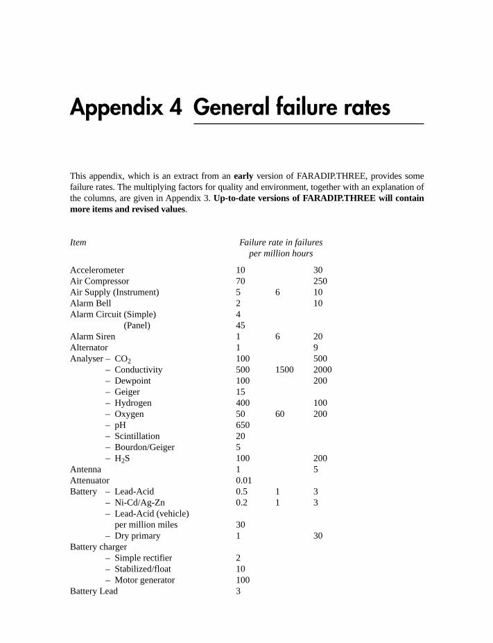
Appendix 4 General failure rates
This appendix, which is an extract from an early version of FARADIP.THREE, provides somefailure rates. The multiplying factors for quality and environment, together with an explanation ofthe columns, are given in Appendix 3. Up-to-date versions of FARADIP.THREE will containmore items and revised values.
Item Failure rate in failures per million hours
Accelerometer 10 30Air Compressor 70 250Air Supply (Instrument) 5 6 10Alarm Bell 2 10Alarm Circuit (Simple) 4
(Panel) 45Alarm Siren 1 6 20Alternator 1 9Analyser – CO2 100 500
– Conductivity 500 1500 2000– Dewpoint 100 200– Geiger 15– Hydrogen 400 100– Oxygen 50 60 200– pH 650– Scintillation 20– Bourdon/Geiger 5– H2S 100 200
Antenna 1 5Attenuator 0.01Battery – Lead-Acid 0.5 1 3
– Ni-Cd/Ag-Zn 0.2 1 3– Lead-Acid (vehicle)
per million miles 30– Dry primary 1 30
Battery charger– Simple rectifier 2– Stabilized/float 10– Motor generator 100
Battery Lead 3

Appendix 4 301
Item Failure rate in failures per million hours
Bearings – Ball, light 0.1 1 10– Ball, heavy 2 20– Roller 0.3 5– Sleeve 0.5 5– Jewel 0.4– Brush 0.5– Bush 0.05 0.4
Bellows, simple expandable 2 5 10Belts 4 50Busbars 11 kV 0.02 0.2
– 3.3 kV 0.05 2– 415 V 0.6 2
Cable (Power) per km– Overhead �600 V 0.5
600–15 kV 5 15�33 kV 3 7
– Underground �600 V 2600–15 kV 2
– Subsea 2.5Capacitors
– Paper 0.001 0.15– Plastic 0.001 0.01 0.05– Mica 0.002 0.03 0.1– Glass 0.002– Ceramic 0.0005 0.1– Tant. sol. 0.005 0.1– Tant. non-sol. 0.001 0.01 0.1– Alumin. (gen.) 0.3– Variable 0.005 0.1 2
Card Reader 150 4000Circuit Breaker
– �600 V or A 0.5 1.5– �3 kV 0.5 2– �100 kV 3 10
Clutch – Friction 0.5 3– Magnetic 2.5 6
Compressor– Centrifugal, turbine driven 150– Reciprocating turbine driven 500– Electric motor driven 100 300
Computer– Mainframe 4000 8000– Mini 100 200 500– Micro (CPU) 30 100– PLC 20 50

302 Reliability, Maintainability and Risk
Item Failure rate in failures per million hours
Connections– Hand solder 0.0002 0.003– Flow solder 0.0003 0.001– Weld 0.002– Wrapped 0.00003 0.001– Crimped 0.0003 0.007– Power cable 0.05 0.4– Plate th. hl. 0.0003
Connectors– Coaxial 0.02 0.2– PCB 0.0003 0.1– pin 0.001 0.1– r.f. 0.05– pneumatic 1– DIL 0.001
Counter (mech.) 0.2 2Crystal, Quartz 0.02 0.1 0.2Detectors
– Gas, pellistor 3 8– Smoke, ionization 2 6– Ultra-violet 5 15– Rate of rise (temp.) 3 9– Temperature level 0.2 2 8– Fire, Wire/rod 10
Diesel Engine 300 6000Diesel Generator 125 4000 (0.97 start)Diodes – Si, high power 0.1 0.2
– Si, low power 0.01 0.04 0.1– Zener 0.005 0.03 0.1– Varactor 0.06 0.3– SCR (Thyristor) 0.01 0.5
Disk Memory 100 500 2000Electricity Supply 100Electropneumatic Converter (I/P) 2 4Fan 2 50Fibre Optics
– Connector 0.1– Cable/km 0.1– LED 0.2 0.5– Laser 0.3 0.5– Si Avalanche photodiode 0.2– Pin Avalanche photodiode 0.02– Optocoupler 0.02 0.1
Filter (Blocked) 0.5 1 10(Leak) 0.5 1 10
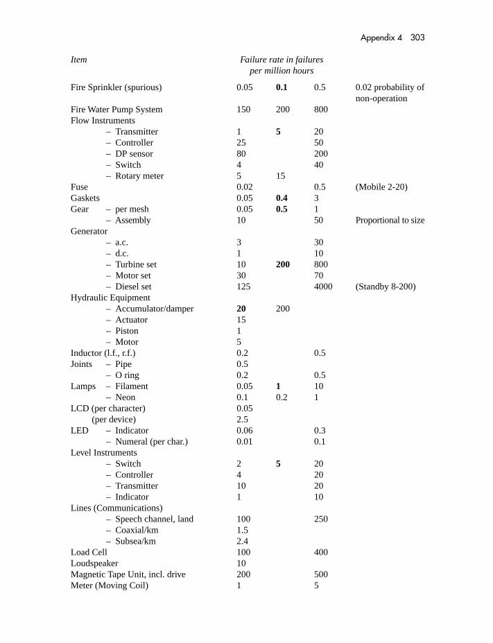
Appendix 4 303
Item Failure rate in failures per million hours
Fire Sprinkler (spurious) 0.05 0.1 0.5 0.02 probability ofnon-operation
Fire Water Pump System 150 200 800Flow Instruments
– Transmitter 1 5 20– Controller 25 50– DP sensor 80 200– Switch 4 40– Rotary meter 5 15
Fuse 0.02 0.5 (Mobile 2-20)Gaskets 0.05 0.4 3Gear – per mesh 0.05 0.5 1
– Assembly 10 50 Proportional to sizeGenerator
– a.c. 3 30– d.c. 1 10– Turbine set 10 200 800– Motor set 30 70– Diesel set 125 4000 (Standby 8-200)
Hydraulic Equipment– Accumulator/damper 20 200– Actuator 15– Piston 1– Motor 5
Inductor (l.f., r.f.) 0.2 0.5Joints – Pipe 0.5
– O ring 0.2 0.5Lamps – Filament 0.05 1 10
– Neon 0.1 0.2 1LCD (per character) 0.05
(per device) 2.5LED – Indicator 0.06 0.3
– Numeral (per char.) 0.01 0.1Level Instruments
– Switch 2 5 20– Controller 4 20– Transmitter 10 20– Indicator 1 10
Lines (Communications)– Speech channel, land 100 250– Coaxial/km 1.5– Subsea/km 2.4
Load Cell 100 400Loudspeaker 10Magnetic Tape Unit, incl. drive 200 500Meter (Moving Coil) 1 5

304 Reliability, Maintainability and Risk
Item Failure rate in failures per million hours
Microwave Equipment– Fixed element 0.01– Tuned element 0.1– Detector/mixer 0.2– Waveguide, fixed 1– Waveguide, flexible 2.5
Motor (Electrical)– a.c. 1 5 20– d.c. 5 15– Starter 4 10
Optodevices See Fibre OpticsPhotoelectric Cell 15Pneumatic Equipment
– Connector 1.5– Controller 1 2 Open or short– Controller 10 20 Degraded– I/P converter 2 10– Pressure relay 20
Power Supply– d.c./d.c. converter 2 5 20– a.c./d.c. stabilized 5 20 100 If possible carry
out FMEAPressure Instruments
– Switch 1 5 40– Sensor 2 10– Indicator 1 5 10– Controller 1 10 30 1 catastrophic, 20
degraded– Transmitter (P/I) (I/P) 5 20
Printed Circuit Boards– Single sided 0.02– Double (plated through) 0.01 0.3– Multilayer 0.07 0.1
Printer (Line) 300 1000Pumps – Centrifugal 10 50 100
– Boiler 100 700– Fire water – diesel 200 3000
– electr. 200 500– Fuel 3 180– Oil lubrication 6 70– Vacuum 10 25
Pushbutton 0.1 0.5 10Rectifier (Power) 3 5Relays – Armature general 0.2 0.4
– Crystal can 0.15– Heavy duty 2 5

Appendix 4 305
Item Failure rate in failures per million hours
Relays – Polarized 0.8– Reed 0.002 0.2 2– BT 0.02 0.07– Contactor 1 6– Power 1 16– Thermal 0.5 10– Time delay 0.5 2 10– Latching 0.02 1.5
Resistors – Carbon comp 0.001 0.006– Carbon film 0.001 0.05– Metal oxide 0.001 0.004 0.05– Wire wound 0.001 0.005 0.5– Networks 0.05 0.1– Variable WW 0.02 0.05 0.5– Variable comp. 0.5 1.5
Solenoid 0.4 1 4Stepper Motor 0.5 5Surge Arresters
– �100 kV 0.5 1.5– low power 0.003 0.02
Switches (per contact)– Micro 0.1 1– Toggle 0.03 1– DIL 0.03 0.5 1.8– Key (low power) 0.003 2
(high power) 5 10– Pushbutton 0.2 1 10– Rotary 0.05 0.5– Thermal Delay 0.5 3
Synchros and Resolvers 3 15Temperature Instruments
– Sensor 0.2 10– Switch 3 20– Pyrometer 250 1000– Transmitter 10– Controller 20 40
Thermionic Tubes– Diode 5 20 70– Triode and Pentode 20 30 100– Thyratron 50
Thermocouple/Thermostat 1 10 20Timer (electromech.) 2 15 40Transformers
– Signal 0.005 0.2 0.3– Mains 0.03 0.4 3– �415 V 0.4 1 7

306 Reliability, Maintainability and Risk
Item Failure rate in failures per million hours
Transistors– Si npn low power 0.01 0.05 0.2– Si npn high power 0.1 0.4– Si FET low power 0.05– Si FET high power 0.1
Turbine, Steam 30 40TV Receiver 2.3 1984 figureValves (Mechanical, Hydraulic,
Pneumatic, Gas (not high temp.nor corrosive substances))
– Ball 0.2 3 10– Butterfly 1 20 30– Diaphragm (single) 2.6 10 20– Gate 1 10 30– Needle 1.5 20– Non-return 1 20– Plug 1 18– Relief 2 8– Globe 0.2 2– Solenoid 1 8 De-energize to trip– Solenoid 8 20 Energize to trip
Valve diaphragm 1 5VDU 10 200 500
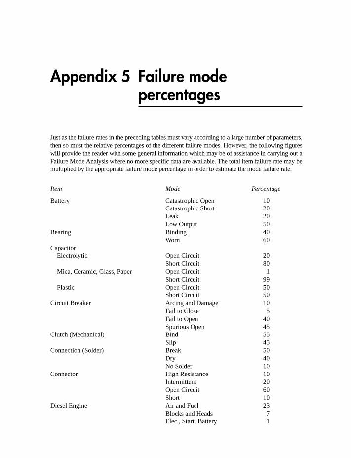
Appendix 5 Failure modepercentages
Just as the failure rates in the preceding tables must vary according to a large number of parameters,then so must the relative percentages of the different failure modes. However, the following figureswill provide the reader with some general information which may be of assistance in carrying out aFailure Mode Analysis where no more specific data are available. The total item failure rate may bemultiplied by the appropriate failure mode percentage in order to estimate the mode failure rate.
Item Mode Percentage
Battery Catastrophic Open 10Catastrophic Short 20Leak 20Low Output 50
Bearing Binding 40Worn 60
CapacitorElectrolytic Open Circuit 20
Short Circuit 80Mica, Ceramic, Glass, Paper Open Circuit 1
Short Circuit 99Plastic Open Circuit 50
Short Circuit 50Circuit Breaker Arcing and Damage 10
Fail to Close 5Fail to Open 40Spurious Open 45
Clutch (Mechanical) Bind 55Slip 45
Connection (Solder) Break 50Dry 40No Solder 10
Connector High Resistance 10Intermittent 20Open Circuit 60Short 10
Diesel Engine Air and Fuel 23Blocks and Heads 7Elec., Start, Battery 1

308 Reliability, Maintainability and Risk
Item Mode Percentage
Lube and Cooling 23Misc. and Seals 16Moving Mech. Parts 30
Diode (Junction) High Reverse 60Open 25Short 15
Diode (Zener) Open 50Short 50
Fuse Fails to Open 15Opens 10Slow to Open 75
Gear Binding 80No Transmission 20
Generator Drift or Intermittent 80Loss of Output 20
Inductor Open 75Short 25
Lamp Open 100Meter (Moving Coil) Drift 30
No Reading 70Microelectronics (digital) o/p high or low 80
loss of function 20Microelectronics (linear) output frozen 20
drift 20o/p max 30o/p min (zero) 30
Motor Failed – Brush 15– Commutator 10– Lube 15 65– Rotor 10– Stator 15
Performance (Degraded)– Brush 15– Commutator 5 35– Lube 15
Pump Leak 50No Transmission 50
Relay Coil 10Contact 90
Relay, Contact Fail to Operate 90Fail to Release 10
Resistor (Comp.) Open 50Drift 50
(Film) Open 50Drift 50
�
�

Appendix 5 309
Item Mode Percentage
(Var.) Open 40Intermittent 60
(Wire) Open 90Short 10
SCR Open 2Short 98
Switch (Micro) High Resistance 60No Function 10Open 30
(Pushbutton) Open 80Short 20
Transformer Open – Primary 5060
– Secondary 10Short – Primary 30 40
– Secondary 10Transistor High Leakage 20
Low Gain 20Open Circuit 30Short Circuit 30
Valve (Mechanical) Blocking 5External Leak 15Passing (Internal) 60Sticking 20
Valve Actuator Fail 10Spurious 90
Note: Can be Spurious Open or Spurious Close, Fail Open or Fail Close, depending on the hydraulic logic
��

Appendix 6 Human error rates
In more general Reliability work, risk analysis is sometimes involved. Also, system MTBFcalculations often take account of the possibilities of human error. A number of studies have beencarried out in the UK and the USA which attempt to quantify human error rates. The following isan overview of the range of error rates which apply.
It must be emphasized that these are broad guidelines. In any particular situation thehuman-response reliability will be governed by a number of shaping factors which include:
Environmental factors – Physical– Organizational– Personal
Intrinsic error – Selection of Individuals– Training– Experience
Stress factors – Personal– Circumstantial
Error rate (per task)Read/ Physical Everyday reason operation yardstick
Simplest possible taskFail to respond to annunciator 0.0001Overfill bath 0.00001Fail to isolate supply (electrical work) 0.0001Read single alphanumeric wrongly 0.0002Read 5-letter word with good resolution wrongly 0.0003Select wrong switch (with mimic diagram) 0.0005Fail to notice major cross-roads 0.0005
Routine simple taskRead a checklist or digital display wrongly 0.001Set switch (multiposition) wrongly 0.001Calibrate dial by potentiometer wrongly 0.002Check for wrong indicator in an array 0.003Wrongly carry out visual inspection for
a defined criterion (e.g. leak) 0.003Fail to correctly replace PCB 0.004Select wrong switch among similar 0.005

Appendix 6 311
Error rate (per task)Read/ Physical Everydayreason operation yardstick
Read analogue indicator wrongly 0.005Read 10-digit number wrongly 0.006Leave light on 0.003
Routine task with care neededMate a connector wrongly 0.01Fail to reset valve after some related task 0.01Record information or read graph wrongly 0.01Let milk boil over 0.01Type or punch character wrongly 0.01Do simple arithmetic wrongly 0.01–0.03Wrong selection – vending machine 0.02Wrongly replace a detailed part 0.02Do simple algebra wrongly 0.02Read 5-letter word with poor resolution wrongly 0.03Put 10 digits into calculator wrongly 0.05Dial 10 digits wrongly 0.06
Complicated non-routine taskFail to notice adverse indicator when reaching
for wrong switch or item 0.1Fail to recognize incorrect status in roving
inspection 0.1New workshift – fail to check hardware, unless
specified 0.1General (high stress) 0.25Fail to notice wrong position of valves 0.5Fail to act correctly after 1 min in emergency
situation 0.9
In failure rate terms the incident rate in a plant is likely to be in the range of 20 � 10�6 per h(general human error) to 1 � 10�6 per h (safety-related incident).

Appendix 7 Fatality rates
The following are approximate fatality rates for the UK (summarized from numerous sources)for a number of Occupational, Voluntary, Involuntary and Travel risks. They are expressed asrates, which for small values may be taken as probabilities, on the basis of annual and exposedhours. A rate per year expresses the probability of an individual becoming a fatality in one year,given a normal exposure to the risk in question. A FAFR (Fatal Accident Frequency Rate) isexpressed on the basis of the number of expected fatalities per 100 million exposed hours.
Per year FAFR Other
TravelAir (Scheduled) 2 � 10�6 1 � 10�7 per landing
or 5 � 10�5 per lifetimeor 2 � 10�10 per km
Train 3 � 10�6 3–5 1 � 10�9 per kmBus 1 � 10�4 4 5 � 10�10 per kmCar 0.5 � 10�4 50–60 c. 3500 per year
4 � 10�10 per kmCanoe 650Gliding 1000Motor cycle 2 � 10�2 500–1050 10�7 per kmWater (General) 2 � 10�6 9 � 10�9 per km
OccupationBritish Industry 2–4 (USA 7) c. 800 per year (UK)Chemical Industry 5 � 10�5 4Construction 1 � 10�4
Construction Erectors 10–70Mining (Coal) 1 � 10�4 10 (USA 30)Nuclear 4 � 10�5
Railway Shunting 2 � 10�4 45Boxing 20 000Steeplejack 300Boilers (100% exposure) 3 � 10�5 0.3Agriculture 7 � 10�5 10 (USA 3)Mechanical, Manufacturing 8Oil and gas extraction 1 � 10�3
Furniture 3Clothing/Textiles 2 � 10�5 0.2Electrical Engineering 1 � 10�5
Shipping 9 � 10�4 8 c. 250 per year

Appendix 7 313
Per year FAFR Other
VoluntarySmoking (20 per day) 500 � 10�5
Drinking (3 pints per day) 8 � 10�5
Football 4 � 10�5
Car Racing 120 � 10�5
Rock Climbing 14 � 10�5 4000 4 � 10�5 per hourThe Pill 2 � 10�5
Swimming 1300
InvoluntaryEarthquake, UK 2 � 10�8
Earthquake, California 2 � 10�6
Lightning (in UK) 1 � 10�7
Skylab strike 5 � 10�12
Pressure vessels 5 � 10�8
Nuclear (1 km) 1 � 10�7
Run over 6 � 10�5
Falling aircraft 2 � 10�8
Venomous bite 2 � 10�7
Petrol/chemical transport 2 � 10�8 1 in 670 million milesLeukaemia 8 � 10�5
Influenza 2 � 10�4
Meteorite 6 � 10�11
Firearms/explosive 1 � 10�6
Homicide 1 � 10�5
Drowning 1 � 10�5
Fire 2 � 10�5
Poison 1.5 � 10�5
Suicide 8 � 10�5
Falls 1 � 10�4
Staying at Home 1–4All accidents 4 � 10�4
Electrocution 1.2 � 10�6
Cancer 25 � 10�4
All accidents 3 � 10�4
Natural disasters (general) 2 � 10�6
All causes* 1 � 10�2
* See A Healthier Mortality ISBN 0-952 5072-1-8.

Appendix 8 Answers to exercises
Chapter 2
(a) (b)
1. 114 1.12. 0.99 0.42 (0.12*)3. 10�5 10�3
4. 2.2 � 10�3 0.18 (0.22*)5. Negligible Negligible6. Unavailability � 2 Unavailability � 2
* Beware the approximation. �t is large (i.e. 0.876). Furthermore, if the 10 000 hr per year approximationwere used, then �t � 1.
Chapter 5
1. Accumulated time T � 50 � 100 � 5000 h. Since the test was time truncated n � 2(k � 1).Therefore,(a) n � 6, T � 5000, � � 0.4. From Appendix 2, �2 � 6.21
(b) n � 2, T � 5000, � � 0.4. From Appendix 2, �2 � 1.83
2. If k � 0 then n � 2 and since confidence level � 90% � � 0.1Therefore �2 � 4.61
Since there are 50 devices the duration of the test is 11 525
50� 231 h.
Therefore T �5000 � 4.61
2� 11 525 h
MTBF90% � 5000 �2T
�2 �2T
4.61
MTBF60% �2T
�2 �10 000
1.83� 5464 h
MTBF60% �2T
�2 �10 000
6.21� 1610 h

Appendix 8 315
3. From Figure 5.7. If c � 0 and P0�c � 0.85 (� � 0.15) then m � 0.17
Therefore T � m � 0.17 � 1000 � 170 h
If MTBF is 500 h then m � T/ � 170/500 � 0.34 which shows � 70%
If c � 5 then m � 3.6 at P0�c � 0.85
Therefore T � m � 3.6 � 1000 � 3600 h
If MTBF is 500 h then m � T/ � 3600/500 � 7.2 which shows � 28%
NB: Do not confuse � meaning (1 – confidence level) with � as producer’s risk.
Chapter 6
1. From the example
If R(t) � 0.95
Therefore 1.5 log (t/1110) � log 0.051
Therefore log (t/1110) � �1.984
Therefore t/1110 � 0.138
Therefore t � 153 h
2. Using the table of median ranks, sample size 10, as given in Chapter 6, plot the data andverify that a straight line is obtained.
Note that � 2 and that � � 13 000 h
Therefore
and
MTBF � 0.886 � 13 000 � 11 500 h
Chapter 7
1. R(t) � e��t [2e��t � e�2�t]
� 2e�2�t � e�3�t
NB: Not a constant failure rate system despite � being constant.
MTBF � ��
0
R(t) dt �1
��
1
3��
2
3�
R(t) � exp�� �t
13 000�2�
Then � t
1110�1.5
� 0.051
R(t) � �� �t
1110 �1.5�

316 Reliability, Maintainability and Risk
2. This is a conditional redundancy problem. Consider the reliability of the system if (a) B doesfail and (b) B does not fail. The following two block diagrams describe the equivalent systemsfor these two possibilities.
Using Bayes theorem the reliability is given as:
Reliability of diagram (a) � probability that B fails (i.e. 1 � Rb)PLUS
Reliability of diagram (b) � probability that B does not fail (i.e. Rb)
Therefore System Reliability
� [RaRd � RcRe � RaRdRcRe] (1 � Rb) � [Rd � Re � RdRe] Rb
Chapter 9
1(a) Loss of supply – Both streams have to fail, i.e. the streams are in parallel, hence the reliabilityblock diagram is
R � 1 � (1 � Rs) (1 � Rs)
where Rs is the reliability of each stream from Section 7.3
R � 1 � (1 � 0.885) (1 � 0.885) � 0.9868
1(b) Overpressure – occurs if either stream fails open, hence the streams are in series from areliability point of view, and the block diagram is:

Appendix 8 317
R � Rs2 where Rs is the reliability of each stream from Section 7.4.2
R � (0.999)2 � 0.998
Notes
The twin stream will reduce the risk of loss of supply, but increase the risk of over-pressure.The same principles can be used to address more realistic complex systems with non-return
valves, slam shuts pressure transducers, etc.R will be increased if loss of supply in one stream can be detected and repaired while the other
stream supplies. The down time of a failed stream is then relevant to the calculation and different.
2(a)
� (Stream) � �1 � �2 � 14 � 10�6 ph
Thus:
Failure Rate � 2�2MDT where MDT � of 2 weeks
� 2(14 � 10�6)2 � 168
� 0.0659 � 10�6
MTBF � 1/� � 1733 years
2(b)
1
2
14
14
0.705

318 Reliability, Maintainability and Risk
Failure Rate � 0.0659 � 10�6 � 0.705 � 10�6
� 0.7709 � 10�6
MTBF � 1/� � 148 years.
3.
The overall Unavailability is 0.01. Calculating the Unavailability for each cutset:
MOTOR 0.0084 (84%)PUMP 0.00144 (14%)PSU and STANDBY 0.0002 (2%)UV DETECTOR and PANEL (negl)
Note that the ranking, and the percentage contributions, are not the same as for failure rate.
Chapter 12
1.
Cumulative hours Failures Anticipated Deviation Cusum
3 000 1 1 0 06 000 2 1 1 19 000 2 1 1 2
12 000 1 1 0 215 000 2 1 1 318 000 0 1 �1 221 000 1 1 0 224 000 2 1 1 327 000 1 1 0 330 000 1 1 0 333 000 2 1 1 436 000 2 1 1 539 000 0 1 �1 442 000 1 1 0 445 000 0 1 �1 348 000 0 1 �1 251 000 0 1 �1 154 000 0 1 �1 057 000 0 1 �1 �160 000 0 1 �1 �2
2.
T1 � 50 � 8760 � 0.25 � 109 500
1 � 109 500/20 � 5475 hrs
T2 � 109 500 � 100 � 8760 � 0.25 � 328 500

Appendix 8 319
2 � 328 500/35 � 9386 hrs
2/1 � (T2/T1)� Therefore 1.714 � 3� Therefore � � 0.5
� k T� So 5475 � k � 331 Therefore k � 16.5
For MTBF to be 12 000, T 0.5 � 12 000/16.5 so T � 528 900 hours.
Which is another 200 400 hours.
Which will take c. 2000 hours with the number on trial.
If � � 0.6, k changes as follows:
k (328 500)0.6 � 9386 Therefore k � 4.6
Now MTBF is 12 000 at T 0.6 � 12 000/4.6 so T � 491 800 hours.
Which is another 163 300 hours.
Which will take c. 1600 hours with the number on trial.

Appendix 9 Bibliography
BOOKS
Carter, A. D. S., Mechanical Reliability, 2nd edn, Macmillan, London (1986).Collins, J. A., Failure of Materials in Mechanical Design, Wiley, New York (1981).Fullwood, R. F., Probabilistic Safety Assessment in the Chemical and Nuclear Industries,
Butterworth-Heinemann, Oxford (1999) ISBN 0 7506 7208 0.Goldman, A. S. and Slattery, T. B., Maintainability – A Major Element of System Effectiveness,
Wiley, New York (1964).Jensen, F. and Petersen, N. E., Burn In, Wiley, New York (1982).Kapur, K. C. and Lamberson, L. R., Reliability in Engineering Design, Wiley, New York (1977).Kivensen, G., Durability and Reliability in Engineering Design, Pitman, London (1972).Moubray, J., Reliability-centred Maintenance, Butterworth-Heinemann, Oxford (1997)
ISBN 0 7506 3358 1.Myers, G. J., Software Reliability, Principles and Practice, Wiley, New York (1976).O’Connor, P. D. T. O., Practical Reliability Engineering, 3rd edn, Wiley, Chichester (1991).Shooman, M., Software Engineering – Reliability, Design, Management, McGraw-Hill,
New York (1984).Smith, C. O., Introduction to Reliability in Design, McGraw-Hill, New York (1976).Smith, D. J., Statistics Workshop, Technis, Tonbridge (1991) ISBN 0 9516562 0 1.Smith, D. J., Achieving Quality Software, 3rd edn, Chapman Hall, London (1995)
ISBN 0 412 62270X.Smith and Simpson, Functional Safety: A Straightforward Guide to IEC 61508, 2nd edn,
Butterworth-Heinemann, Oxford (2001) ISBN 07506 6269 7.Snedecor, G. W. and Cochran, W. G., Statistical Methods, Ames, Iowa State University Press
(1967).Whittingham, R. B., The Blame Machine, Elsevier ISBN 07506 5510-0.
OTHER PUBLICATIONS
Human Reliability Assessors Guide (SRDA-R11), June 1995, UKAEA, Thomson House,Risley, Cheshire WA3 6AT ISBN 085 3564 205.
Nomenclature for Hazard and Risk Assessment in the Process Industries, 1985 (reissued 1992),IChemE, 165–171 Railway Terrace, Rugby, CV21 3HQ ISBN 0852951841.
Tolerability of Risk for Nuclear Power Stations, UK Health and Safety Executive,ISBN 0118863681.
HSE, 1999, Reducing Risks Protecting People. HSE’s decision making forces HSE Books.HAZOP – A Guide to Hazard and Operability Studies, 1977, Chemical Industries Association,
Alembic House, 93 Albert Embankment, London SE1 7TU.

Appendix 9 321
A Guide to the Control of Industrial Major Accident Hazards Regulations, HMSO, London(1984).
UPM3.1: A Pragmatic Approach to Dependent Failures Assessment for Standard Systems,UK AEA, ISBN 0853564337.
Technis Guidelines Q124, Demonstration of Product/System Compliance with IEC 61508ISBN 0951 6562 79.
STANDARDS AND GUIDELINES
BS 2011 Basic environmental testing procedures.BS 4200 Guide on the reliability of electronic equipment and parts used therein.BS 4778 Glossary of terms used in quality assurance (Section 3.2: 1991 is Reliability).BS 5760 Reliability of systems, equipment and components.BS 6651: 1990 Code of practice for protection of structures against lightning.UK DEF STD 00-40 Reliability and maintainability.UK DEF STD 00-41 MOD Practices and procedures in reliability and maintainability.UK DEF STD 00-55 The procurement of safety critical software in defence equipment.UK DEF STD 00-56 Hazard analysis and safety classification of the computer and programmable
electronic system elements of defence equipment.UK DEF STD 00-58 A Guideline for HAZOP studies on systems which include programmable
electronic systems.UK DEF STD 07-55 Environmental testing.US Military Handbook 217E (Notice 1) Reliability Prediction of Electronic Equipment, 1990.US Military Handbook 338 Electronic Reliability Design Handbook.US Military Standard 470 Maintainability programme requirements, 1966.US Military Standard 471A Maintainability/Verification/Demonstration/Evaluation, 1973.US Military Handbook 472 Maintainability Prediction, 1966.US Military Standard 721B Definitions of Effectiveness Terms for Reliability.US Military Standard 756 Reliability Prediction.US Military Standard 781C Reliability Design Qualification and Production Acceptance Tests.US Military Standard 785A Reliability Programme for Systems and Equipment Development
and Production, 1969.US Military Standard 810 Environmental Test Methods.US Military Standard 883 Test Methods and Procedures for Microelectronic Devices.US Military Standard 1629A Procedures for Performing a Failure Mode, Effects and Criticality
Analysis.US Military Standard 52779 (AD) Software Quality Assurance Requirements.IGEM Publication SR15, Programmable Equipment in Safety Related Applications (4th edition
2005) ISBN 0717700739.IGEM Publication SR24, Risk Assessment Techniques (1998) ISBN 0717700933.IEE, Competency Guidelines for Safety Related Systems Practitioners, 1999, ISBN 085296787X.IEC Publication 271, Preliminary List of Basic Terms and Definitions for the Reliability of
Electronic Equipment and Components (or parts) used therein.IEC61508 Functional Safety: Safety Related Systems – 7 Parts.IEC International Standard 61511: Functional Safety – Safety Instrumented Systems for the
Process Industry Sector.IEEE Standard 500, Reliability Data for Pumps, Drivers, Valve Actuators and Valves, 1994,
Library of Congress 83–082816.

322 Reliability, Maintainability and Risk
European Standard BSEN 51026: Railway Applications – The Specification and Demonstrationof Dependability, Reliability, Maintainability and Safety (RAMS).
RTCA DO–178B/(EUROCAE ED–12B) – Software Considerations in Airborne Systems andEquipment Certification.
UKOOA: Guidelines for Process Control and Safety Systems on Offshore Installations.
JOURNALS
Journal of the Safety and Reliability Society (quarterly).Quality and Reliability International, Wiley (quarterly).Microelectronics and Reliability (Pergamon Press).US IEEE Transactions on Reliability.

Appendix 10 Scoring criteria forBETAPLUS commoncause model
1 CHECKLIST AND SCORING FOR EQUIPMENT CONTAININGPROGRAMMABLE ELECTRONICS
Score between 0 and 100% of the indicated maximum values.
(1) SEPARATION/SEGREGATION A Max B Maxscore score
Are all signal cables separated at all positions? 15 52
Are the programmable channels on separate printed circuit boards? 85 55
OR are the programmable channels in separate racks? 90 60
OR in separate rooms or buildings? 95 65
MAXIMUM SCORE 110 117
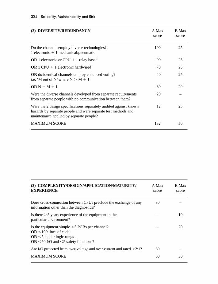
324 Reliability, Maintainability and Risk
(2) DIVERSITY/REDUNDANCY A Max B Maxscore score
Do the channels employ diverse technologies?; 100 251 electronic � 1 mechanical/pneumatic
OR 1 electronic or CPU � 1 relay based 90 25
OR 1 CPU � 1 electronic hardwired 70 25
OR do identical channels employ enhanced voting? 40 25i.e. ‘M out of N’ where N � M � 1
OR N � M � 1 30 20
Were the diverse channels developed from separate requirements 20 –from separate people with no communication between them?
Were the 2 design specifications separately audited against known 12 25hazards by separate people and were separate test methods andmaintenance applied by separate people?
MAXIMUM SCORE 132 50
(3) COMPLEXITY/DESIGN/APPLICATION/MATURITY/ A Max B Max EXPERIENCE score score
Does cross-connection between CPUs preclude the exchange of any 30 –information other than the diagnostics?
Is there �5 years experience of the equipment in the – 10particular environment?
Is the equipment simple �5 PCBs per channel? – 20OR �100 lines of codeOR �5 ladder logic rungsOR �50 I/O and �5 safety functions?
Are I/O protected from over-voltage and over-current and rated �2:1? 30 –
MAXIMUM SCORE 60 30

Appendix 10 325
(4) ASSESSMENT/ANALYSIS and FEEDBACK of DATA A Max B Max score score
Has a combination of detailed FMEA, Fault Tree analysis and design – 140review established potential CCFs in the electronics?
Is there documentary evidence that field failures are fully analysed – 70with feedback to design?
MAXIMUM SCORE – 210
(5) PROCEDURES/HUMAN INTERFACE A Max B Max score score
Is there a written system of work on site to ensure that failures are 30 20investigated and checked in other channels? (including degradeditems which have not yet failed)
Is maintenance of diverse/redundant channels staggered at such an 60 –interval as to ensure that any proof-tests and cross-checks operatesatisfactorily between the maintenance?
Do written maintenance procedures ensure that redundant separations 15 25as, for example, signal cables are separated from each other and frompower cables and must not be re-routed?
Are modifications forbidden without full design analysis of CCF? – 20
Is diverse equipment maintained by different staff? 15 20
MAXIMUM SCORE 120 85
(6) COMPETENCE/TRAINING/SAFETY CULTURE A Max B Maxscore score
Have designers been trained to understand CCF? – 100
Have installers been trained to understand CCF? – 50
Have maintainers been trained to understand CCF? – 60
MAXIMUM SCORE – 210

326 Reliability, Maintainability and Risk
(7) ENVIRONMENTAL CONTROL A Max B Maxscore score
Is there limited personnel access? 40 50
Is there appropriate environmental control? (e.g. temperature, 40 50humidity)
MAXIMUM SCORE 80 100
(8) ENVIRONMENTAL TESTING A Max B Maxscore score
Has full EMC immunity or equivalent mechanical – 316testing been conducted on prototypes and productionunits (using recognized standards)?
MAXIMUM SCORE – 316
A Max B Maxscore score
TOTAL MAXIMUM SCORE 502 1118

Appendix 10 327
2 CHECKLIST AND SCORING FOR NON-PROGRAMMABLE EQUIPMENT
Only the first three categories have different questions as follows:
(1) SEPARATION/SEGREGATION A Max B Max score score
Are the sensors or actuators physically separated 15 52and at least 1 metre apart?
If the sensor/actuator has some intermediate electronics 65 35or pneumatics, are the channels on separate PCBs and screened?
OR if the sensor/actuator has some intermediate electronics or 95 65pneumatics, are the channels indoors in separate racks or rooms?
MAXIMUM SCORE 110 117
(2) DIVERSITY/REDUNDANCY A Max B Max score score
Do the redundant units employ different technologies?; 100 25e.g. 1 electronic or programmable � 1 mechanical/pneumatic
OR 1 electronic, 1 relay based 90 25
OR 1 PE, 1 electronic hardwired 70 25
OR do the devices employ ‘M out of N’ voting where; N � M � 1 40 25
OR N � M � 1 30 20
Were separate test methods and maintenance applied 32 52by separate people?
MAXIMUM SCORE 132 50

328 Reliability, Maintainability and Risk
(3) COMPLEXITY/DESIGN/APPLICATION/MATURITY/ A Max B MaxEXPERIENCE score score
Does cross-connection preclude the exchange of any information 30 –other than the diagnostics?
Is there �5 years experience of the equipment in the particular – 10environment?
Is the equipment simple e.g. non-programmable type – 20sensor or single actuator field device?
Are devices protected from over-voltage and over-current and rated 30 –�2:1 or mechanical equivalent?
MAXIMUM SCORE 60 30
(4) ASSESSMENT/ANALYSIS and FEEDBACK OF DATAAs for Programmable Electronics (see above)
(5) PROCEDURES/HUMAN INTERFACEAs for Programmable Electronics (see above)
(6) COMPETENCE/TRAINING/SAFETY CULTUREAs for Programmable Electronics (see above)
(7) ENVIRONMENTAL CONTROLAs for Programmable Electronics (see above)
(8) ENVIRONMENTAL TESTINGAs for Programmable Electronics (see above)
A Max B Maxscore score
TOTAL MAXIMUM RAW SCORE (Both programmable 502 1118and non-programmable lists)
The diagnostic interval is shown for each of the two (programmable and non-programmable)assessment lists. The (C) values have been chosen to cover the range 1–3 in order to construct amodel which caters for the known range of BETA values.

Appendix 10 329
For Programmable Electronics
Interval Interval Interval Interval�1 min 1–5 mins 5–10 mins �10 mins
Diagnostic coverage98% 3 2.5 2 190% 2.5 2 1.5 160% 2 1.5 1 1
For Sensors and Actuators
Interval Interval Interval Interval�2 hrs 2 hrs–2 days 2 days–1 week �1 week
Diagnostic coverage98% 3 2.5 2 190% 2.5 2 1.5 160% 2 1.5 1 1
A score of C � 1 may only be proposed if the resulting action, initiated by the diagnostics, hasthe effect of preventing or invalidating the effect of the subsequent CCF failure. For example, insome process industry equipment, even though the first of the CCF failures was diagnosedbefore the subsequent failure, there would nevertheless be insufficient time to take action tomaintain the process. The subsequent (second) CCF failure would thus occur before effectiveaction could be taken. Therefore, in such a case, the diagnostics would not help in defendingagainst CCF and a C � 1 score cannot be proposed in the assessment.
AVAILABLE IN SOFTWARE FORM AS BETAPLUS FROM THE AUTHOR AT TECHNIS01732 352532

Appendix 11 Example of HAZOP
Sour gas consisting mainly of methane (CH4) but with 2% hydrogen sulphide (H2S) is routedto an amine absorber section for sweetening. The absorber uses a 25:75% diethanolamine(amine)/water solution to remove the H2S in the absorber tower. Sweet gas is removedfrom the tower top and routed to fuel gas. Rich amine is pressurized from the tower bottomunder level control and then routed to an amine regeneration unit on another plot.Regenerated amine is returned to the amine absorber section and stored in a low-pressurebuffer storage tank.
A11.1 EQUIPMENT DETAILS
Absorber tower operating pressure � 20 bar gauge.The buffer storage tank is designed for low pressure, with weak seam roof and additional relief
provided by a hinged manhole cover.
A11.2 HAZOP WORKSHEETS
The HAZOP worksheets with this example will demonstrate the HAZOP method for just onenode, i.e. the line from the buffer storage tank to the absorber tower.
Nodes that could have been studied in more detail are:
� amine buffer tank� line to absorber tower from amine buffer tank� sour gas line to absorber tower� absorber tower� sweet gas line out of absorber tower� rich amine line out of absorber tower.
A11.3 POTENTIAL CONSEQUENCES
The importance of the consequences identified for a process deviation, and how these are used tojudge the adequacy of safeguards, cannot be over emphasized. In this example, the consequencesof reverse flow include:
� possible tank damage� release of a flammable gas near a congested unit which could lead to an explosion� release of a highly toxic gas.
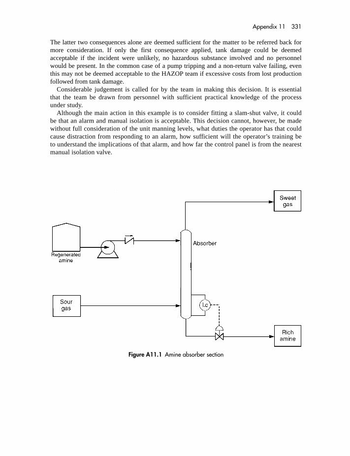
Appendix 11 331
The latter two consequences alone are deemed sufficient for the matter to be referred back formore consideration. If only the first consequence applied, tank damage could be deemedacceptable if the incident were unlikely, no hazardous substance involved and no personnelwould be present. In the common case of a pump tripping and a non-return valve failing, eventhis may not be deemed acceptable to the HAZOP team if excessive costs from lost productionfollowed from tank damage.
Considerable judgement is called for by the team in making this decision. It is essentialthat the team be drawn from personnel with sufficient practical knowledge of the processunder study.
Although the main action in this example is to consider fitting a slam-shut valve, it couldbe that an alarm and manual isolation is acceptable. This decision cannot, however, be madewithout full consideration of the unit manning levels, what duties the operator has that couldcause distraction from responding to an alarm, how sufficient will the operator’s training beto understand the implications of that alarm, and how far the control panel is from the nearestmanual isolation valve.
Figure A11.1 Amine absorber section
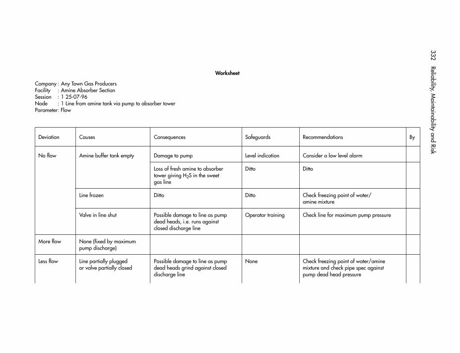
332Reliability, M
aintainability and Risk
Deviation Causes Consequences Safeguards Recommendations By
No flow Amine buffer tank empty Damage to pump Level indication Consider a low level alarm
Loss of fresh amine to absorber Ditto Dittotower giving H2S in the sweetgas line
Line frozen Ditto Ditto Check freezing point of water/amine mixture
Valve in line shut Possible damage to line as pump Operator training Check line for maximum pump pressuredead heads, i.e. runs againstclosed discharge line
More flow None (fixed by maximumpump discharge)
Less flow Line partially plugged Possible damage to line as pump None Check freezing point of water/amineor valve partially closed dead heads grind against closed mixture and check pipe spec against
discharge line pump dead head pressure
Worksheet
Company : Any Town Gas ProducersFacility : Amine Absorber SectionSession : 1 25-07-96Node : 1 Line from amine tank via pump to absorber towerParameter: Flow

Appendix 11
333
Reverse flow Pump trips Back flow of 20 bar gas to Non-return valve (which In view of the potential consequence ofamine tank may not be reliable in the release and its likelihood, undertake
amine service) a full study of the hazards involved, andsafeguards appropriate to these hazardsproposed (possibly installing a choppervalve to cut in and prevent back flow)
Resulting in:1. Possible rupture of tank Tank weak seam Ditto2. Major H2S release to plant None Ditto
causing potential toxic cloud and possible vapour cloud explosion if cloud reaches congested part of the plant
High Failure of cooling on the Possibility of poor absorber Temperature alarm ontemperature amine regeneration unit tower efficiency amine regeneration unit
resulting in hot amine inamine tank
Low Cold conditions Possible freezing of line None at present – but seetemperature action under ‘No flow’ to
investigate freezing point
High pressure Pump dead head Possibility of overpressure of pipe None – but see action under ‘No flow’ to check pipe spec
Reverse flow from Ditto None In previous action to check pipe spec absorber tower against pump dead head pressure also
include checking spec against operatingpressure in absorber tower
Low pressure None identified Not seen as a problem Line good for vacuum Noneconditions

Appendix 12 HAZID checklist
1. Acceleration/shock Change in velocity, 1. Structural deformationimpact energy of 2. Breakdown by impactvehicles, components 3. Displacement of parts or pipingor fluids 4. Seating or unseating valves or
electrical contacts5. Loss of fluid pressure head
(cavitation)6. Pressure surges in fluid systems7. Disruption of metering equipment
2. Chemical energy Chemical disassociation 1. Fireor replacement of fuels, 2. Explosionoxidizers, explosives, 3. Non-explosive exothermic reactionorganic materials or 4. Material degradationcomponents 5. Toxic gas production
6. Corrosion fraction production7. Swelling of organic compounds
3. Contamination Producing or introducing 1. Clogging or blocking of componentscontaminants to surfaces, 2. Friction between moving surfacesorifices, filters, etc. 3. Deterioration of fluids
4. Degradation of performance sensorsor operating components
5. Erosion of lines or components6. Fracture of lines or components by
fast moving large particles
4. Electrical energy System or component 1. Electrocutionpotential energy 2. Involuntary personnel reactionrelease or failure. 3. Personnel burnsIncludes shock both 4. Ignition of combustiblesthermal and static 5. Equipment burnout
6. Inadvertent activation of equipmentor ordinance devices
7. Necessary equipment unavailablefor functions or caution andwarning
8. Release on holding devices

Appendix 12 335
5. Human capability Human factors 1. Personal injury due to:including perception, � restricted routesdexterity, life � hazardous locationsupport and error � inadequate visual/audible
warningsPROBABILITY 2. Equipment damage by improper
operation due to: inaccessiblecontrol location inadequatecontrol/display identification
6. Human hazards Conditions that could 1. Personal injury due to:cause skin abrasions, � sharp edges/cornerscuts, bruises, etc. � dangerous heights
� unguarded floor/wall openings
7. Interface/interaction Compatibility between 1. Incompatible materials reactionsystems/subsystems/ 2. Interfacing reactionsfacilities/software 3. Unintended operations caused/
prevented by software
8. Kinetic energy System/component 1. linear impactlinear or rotary motion 2. Disintegration of rotating components
9. Material deformation Degradation of 1. Change in physical or chemicalmaterial by corrosion, propertiesageing, embrittlement, 2. Structural failureoxidation, etc. 3. Delamination of layered material
4. Electrical short circuiting
10. Mechanical energy System/component 1. Personal injury or equipment damagepotential energy such from energy releaseas compressed springs
11. Natural environment Conditions including 1. Structural damage from windlightning, wind, 2. Electrical dischargeprojectiles, thermal, 3. Dimension changes from solarpressure, gravity, heatinghumidity, etc.
12. Pressure System/component 1. Blast/fragmentation from containerpotential energy, overpressure ruptureincluding high/low 2. line/hose whippingor changing pressure 3. Container implosion/explosion
4. System leaks5. Heating/cooling by rapid changes6. Aeroembolism, bends, choking
or shock

336 Reliability, Maintainability and Risk
13. Radiation Conditions including 1. Electronic equipment interferenceelectromagnetic, 2. Human tissue damageionizing, thermal or 3. Charring of organic materialsultraviolet radiation 4. Decomposition of chlorinated
hydrocarbons into toxic gases5. Ozone or nitrogen oxide generation
14. Thermal System/component 1. Ignition of combustiblespotential energy, 2. Ignition of other reactionsincluding high low or 3. Distortion of partschanging temperature 4. Expansion/contraction of solids
or fluids5. Liquid compound stratification6. Personal injury
15. Toxicants Adverse human effects 1. Respiratory system damageof inhalants or ingests 2. Blood system damage
3. Body organ damage4. Skin irritation or damage5. Nervous system effects
16. Vibration/sound System/component 1. Material failureproduced energy 2. Personal fatigue or injury
3. Pressure/shock wave effects4. Loosening of parts5. Chattering of valves or contacts6. Contamination interface

Appendix 13 Markov analysis ofredundant systems
In Chapter 8, it was explained that the traditional use of Markov analysis, in respect of redundantsystems is fundamentally flawed in that repair/down times are not a random process and dependupon earlier events than the one immediately preceding the failure in question. The repair of thesecond failure is dependent on the progress of the first in that a single repair crew will continueto deal with that first failure.
However, up to the point of the second failure occurring the Markov assumption, given thatthere are multiple repair crews, holds good. It is, therefore, reproduced in this Appendix forinterest since it is so frequently referred to in the literature.
The Markov method for calculating the MTTF of a system with repair is to consider the‘states’ in which the system can exist. Figure A13.1 shows a system with two identical unitseach having failure rate � and repair rate (reciprocal of mean down time) �. The system can bein each of three possible states.
State (0) Both units operatingState (1) One unit operating, the other having failedState (2) Both units failed
It is important to remember one rule with Markov analysis, namely, that the probabilities ofchanging state are dependent only on the state itself. In other words, the probability of failure orof repair is not dependent on the past history of the system – not so in real life.
Let Pi(t) be the probability that the system is in state (i) at time t and assume that the initialstate is (0).
Therefore
P0(0) � 1 and P1(0) � P2(0) � 0
�,µ
�,µ
Figure A13.1

338 Reliability, Maintainability and Risk
Therefore
P0(t) � P1(t) � P2(t) � 1
We shall now calculate the probability of the system being in each of the three states attime t � �t. The system will be in state (0) at time t � �t if:
1. The system was in state (0) at time t and no failure occurred in either unit during theinterval �t, or,
2. The system was in state (1) at time t, no further failure occurred during �t, and the failedunit was repaired during �t.
The probability of only one failure occurring in one unit during that interval is simply ��t(valid if �t is small, which it is). Consequently (1 � ��t) is the probability that no failure willoccur in one unit during the interval. The probability that both units will be failure free duringthe interval is, therefore,
(1 � ��t)(1 � ��t) 1 � 2��t
The probability that one failed unit will be repaired within �t is ��t, provided that �t is verysmall. This leads to the equation:
P0(t � �t) � [P0(t) � (1 � 2��t)] � [P1(t) � (1 � ��t) � ��t]
Similarly, for states 1 and 2:
P1(t � �t) � [P0(t) � 2��t] � [P1(t) � (1 � ��t) � (1 � ��t)]
P2(t � �t) � [P1(t) � ��t] � P2(t)
Now the limit as �t 0 of [Pi(t � �t) � Pi(t)]/�t is Pi(t) and so the above yield:
In matrix notation this becomes:
The elements of this matrix can also be obtained by means of a Transition Diagram. Sinceonly one event can take place during a small interval, �t, the transitions between states
�P0
P1
P2� � ��2�
2�
0
�
�(� � �)
�
0
0
0��P0
P1
P2�
P2(t) � P1(t)�
P1(t) � 2�P0(t) � (� � �)P1(t)
P0(t) � �2�P0(t) � �P1(t)

Appendix 13 339
involving only one repair or one failure are considered. Consequently, the transitions (withtransition rates) are:
by failure of either unit
0 12�
1 2�
1 0µ
10 2
2� �
µ
–(� + µ)
–2�
2� �
µ0 1 2
by failure of the remaining active unit,
by repair of the failed unit of state 1.
The transition diagram is:
Finally closed loops are drawn at states 0 and 1 to account for the probability of not changingstate. The rates are easily calculated as minus the algebraic sum of the rates associated with thelines leaving that state. Hence:
A (3 � 3) matrix, (ai,j), can now be constructed, where i � 1, 2, 3; j � 1, 2, 3; ai,j is the char-acter on the flow line pointing from state j to state i. If no flow line exists the correspondingmatrix element is zero. We therefore find the same matrix as before.

340 Reliability, Maintainability and Risk
The MTTF is defined as
The values of T0 and T1 can be found by solving the following:
Since the (3 � 3) matrix is constant we may write
or
or
Taking account of
P0(0) � 1; P1(0) � P2(0) � 0
P0() � P1() � 0; P2() � 1
we may reduce the equation to
� �1
0
1
� � � �2�
2�
0
�
�(� � �)
�
0
0
0
�� T0
T1
T2
�
� P0() � P0(0)
P1() � P1(0)
P2() � P2(0)
� � � �2�
2�
0
�
�(� � �)
�
0
0
0
�� T0
T1
T2
�
� �
0 P0˙ (t) dt
�
0 P1˙ (t) dt
�
0 P2˙ (t) dt
� � � �2�
2�
0
�
�(� � �)
�
0
0
0
�� �
0 P0(t) dt�
0 P1(t) dt�
0 P2(t) dt
�
�
0 � P0
˙ (t)
P1˙ (t)
P2˙ (t)
� dt � � �2�
2�
0
�
�(� � �)
�
0
0
0
� �
0 � P0
P1
P2
� dt
�
0 � P0˙ (t)
P1˙ (t)
P2˙ (t)
� dt � �
0 � �2�
2�
0
�
�(� � �)
�
0
0
0
�� P0
P1
P2
� dt
� T0 � T1
� �
0P0(t) dt � �
0P1(t) dt
� �
0[P
0(t) � P
1(t)] dt
s � �
0R(t) dt

Appendix 13 341
or
�1 � �2�T0 � �T1
0 � 2�T0 � (� � �)T1
1 � �T1
Solving this set of equations
so that
that is,
Hence (see Chapter 8, Section 8.1.2, Table 8.1).�s �2�2
3� � �� 2�2 MDT
s �3� � �
2�2
s � T0 � T1 �1
��
� � �
2�2 �3� � �
2�2
T0 �� � �
2�2 and T11
�

This Page is Intentionally Left Blank

Index
Accelerated step tests, 162, 164Access, 176Accreditation of assessment, 275Accuracy of data, 37, 46Accuracy of prediction, 46 et seq., 128ACMH, 258Active redundancy, 79 et seq.Adjustment, 176Aircraft impact, 137ALARP, 28, 29, 128, 129, 130 et seq., 269, 285Allocation of reliability, 90, 145, 236Appraisal costs, 30 et seq.Architectures, 285Arrhenius equation, 148Assessment costs, 27 et seq.Auto-test, 99, 115Availability, 21, 25 et seq.
Barlow-Proschan, 106Bathtub Curve, 17 et seq., 163, 217, 242Bayes Theorem, 77, 82Bellcore data, 41Bernard’s approximation, 66BETA method (CCF), 97 et seq.BETAPLUS (CCF), 98 et seq., 323Binomial, 76Boundary model (CCF), 98BS 4200, 22BS 4778, 22BS 5760, 240BS 6651, 137BS 9400, 155Built-in test equipment, 177Burn-in, 18, 155
Cause consequence analysis (see Event trees)Certification, 274Certifying body, 275Change control, 222Chi-square, 51 et seq., 294
in summary, 54CIMAH regulations, 259, 264CNET, 41COMAH, 259, 264
Common Cause/Common Mode Failures, 96 et seq.,106, 115, 323
Company specific data, 39, 46 et seq.COMPARE package, 67, 195, 211, 212Complexity, 7, 153Condition monitoring, 214Conditional redundancy, 82Confidence levels, 46, 50 et seq., 70
double-sided, 53of reliability prediction, 49, 130
Connections, 177Consequence analysis, 132 et seq.Consumer Protection Act, 253Consumer’s risk, 55 et seq., 205Continuous processes, 70Contracts, 10, 241 et seq., 279CORE-DATA, 122Cost, 24 et seq.Cost per life saved, 28, 29, 128, 131CUSUM, 71, 163Cutset ranking, 106Cutsets, 104 et seq.
Data collection, 118, 167 et seq.Data sources, 39 et seq.Defence Standards:
00–40, 24000–56, 273
Definitions, 11 et seq., 286 et seq.Demonstration:
maintainability, 196 et seq.reliability fixed time, 54 et seq.reliability sequential, 57
Dependent failures (see Common Cause/CommonMode Failures)
Derating, 149Design cycle, 221, 237 (see also RAMS cycle)Design review, 224, 237Diagnostic coverage (and interval), 99, 100, 114 et seq.Discrimination, 55 et seq.Displays, 178Diversity, 97 et seq., 324Documentation Controls, 220Down time, 18 et seq., 91 et seq., 113 et seq.,
176 et seq., 196 et seq.

344 Index
Drenick’s law, 69Duane plot, 71, 165
Earthquake, 140EIReDA data, 42Environmental stress, 150
multipliers, 40, 298testing, 159
EPRI data, 42Event-driven simulation, 123Event trees, 109 et seq.
Failure:codes, 170costs, 30 et seq.definition, 11mechanisms, 150 et seq.probability density function, 15reporting, 167 et seq.
Failure rate:data, 37 et seq.general, 12 et seq., 91 et seq., 298 et seq.human error, 118 et seq., 310microelectronic rates, 298 et seq.ranges, 43 et seq.variable, 61 et seq.
FARADIP.THREE data, 43 et seq., 116, 208Fatality rates, 131, 268, 312 et seq.Fault codes, 170 et seq.Fault tolerance, 224Fault tree analysis, 101 et seq.
cautionary note, 108Field data, 167 et seq.FITS, 13FMEA/FMECA, 90, 116 et seq.Formal methods, 225Functional safety capability, 239 et seq.Fussell–Vesely, 106
GADS, 42Generic data, 39, 46 et seq.Genetic algorithms, 126Geometric mean, 45Gnedenko test of significance, 68Growth, 163 et seq.Guidewords, 133
Handbooks, 183 et seq.HAZAN, 136 et seq.Hazard, 4, 21, 132 et seq., 257 et seq.HAZID, 132 et seq.HAZID checklist, 334HAZOP, 133 et seq., 264, 330 et seq.Health and Safety at Work Act, 253HEART, 119, 124
HFRG, 122High reliability testing, 160HRD, 41HSC, 258HSE, 29, 131, 132, 259 et seq., 265Human error rates, 122, 310 et seq.
I Chem E, 22IEC 271, 22IEC 61508, 22, 239, 267 et seq., 272IEC 61511, 272IEEE500, 42IGE, 273Importance measures, 105Industry specific data, 39, 46 et seq.Inference, 50 et seq.Integration and Test, 224Interchangeability, 180ITEM toolkit, 128
Jelinski Moranda, 219
Laplace Test, 71Least Squares, 68Liability, 244, 251 et seq.Lightning, 137Littlewood Verall, 219Load sharing, 85Location parameter, 61 et seq.Logistics, 194LogNormal, 20LRA, 181
Maintainability, 12, 177 et seq., 196 et seq.Maintenance:
handbooks, 183 et seq.Major incident legislation, 257Major incidents, 257MALPAS, 227Marginal testing, 160Markov, 91, 337 et seq.MAROS, 126Maximum Down Time, 20Maximum Likelihood, 68Mean life, 14Median ranking, 66Mercalli, 140Meteorological factors, 141Microelectronic failure rates, 40 et seq., 298MIL-217, 40MIL 470, 240MIL 471A, 204MIL 472, 197 et seq.MIL 473, 205MIL 721B, 22

Index 345
MIL 781C, 60MIL 785A, 240MIL 883, 155MOD 00–56, 273Modelling, 89 et seq., 119 et seq.Monte Carlo, 123Multiparameter testing, 161Multiple Greek Letter model, 98Musa, 219
NIHHS, 258Normal distribution, 51, 205 et seq.NPRD, 41NUCLARR data, 42, 122NUREG, 42
OC (operating characteristics) curves, 56 et seq., 214Offshore safety, 262OPTAGON, 125Optimum costs, 24 et seq.Optimum discard/replacement, 210Optimum proof-test, 212Optimum spares, 212OREDA, 39, 42
Pareto analysis, 172Partial BETA models (see BETA method (CCF))Partial redundancy, 81 et seq.Perception of risk, 130PFD (Probability of Failure on Demand), 21, 267 et seq.Point estimate, 14, 50 et seq.Prediction:
confidence levels, 46reliability, 75 et seq., 89 et seq.repair time, 176 et seq., 196 et seq.
Prevention costs, 30 et seq.Preventive maintenance, 208 et seq.Preventive replacement, 210Probability:
plotting, 61 et seq.theory, 75 et seq.
Probability density function, 15Producer’s risk, 55 et seq.Product liability, 251 et seq.Product recall, 255 et seq.Production loss, 27, 129Programmable devices, 215Programming standards, 222Project management, 235 et seq.Proof-test interval, 21, 93 et seq.
QRA, 130 et seq.QRCM, 208 et seq.qualification testing, 158Qualitative, 6, 269
Quality costs, 30 et seq.Quality multipliers, 40, 298Quantitative, 6, 269
RADC, 37, 40, 41Rail, 265, 273RAM4 package, 127RAMP, 127RAMS, 3, 8, 75, 235RAMS-cycle, 9, 237Random hardware failures, 269, 283Ranking tables, 66RCM (see QRCM)Redundancy, 79 et seq., 89 et seq., 181Reliability:
assessment costs, 24 et seq.block diagrams, 78 et seq., 89 et seq.definition, 12demonstration, 54 et seq.growth, 163 et seq.prediction, 82 et seq., 89 et seq.
Repair rate, 20, 337 et seq.Repair time, 18 et seq., 93 et seq., 176 et seq., 196 et seq.Risk:
graph, 268perception, 130tolerability, 130
RTCA DO-178B, 274
Safe failure fraction, 269 et seq., 285Safety-integrity levels, 267 et seq., 282Safety monitor, 271Safety-related systems, 266 et seq.Safety reports, 259SAM, 127Scale parameter, 61 et seq.Screening, 155Seeding and tagging, 219Self-certification, 274Sequential testing, 57Series reliability, 78 et seq.Seveso Directive, 258Shape parameter, 61 et seq.Significance, 68Simulation, 123 et seq.SINTEF data, 43Site specific data, 38, 45 et seq.Software failure rate modelling, 218Software quality checklists, 228 et seq.Software reliability, 217 et seq.Spares provisioning, 190 et seq., 212SRD, 42, 119SRD data, 42Standardization, 182Standby redundancy, 83 et seq.Static analysis, 227Step-stress testing, 162
346 Index
Stress analysis, 147Stress protection, 150Stress testing, 162 et seq.Strict liability, 252Structured models, 219Subcontract reliability assessment, 249System Cut-off model, 97
TECHNIS data, 42TESEO, 121, 124Test points, 182Testing, 158 et seq.THERP, 121Third party assessment, 275Thunderstorms, 137
Times to failure, 14, 61 et seq.Transition diagrams, 339 et seq.TTREE package, 105
UKAEA, 42UKOOA guidance, 268, 273Unavailability, 21, 91 et seq., 193
Variable failure rate, 61 et seq.
WASH 1400, 42Wearout, 18, 59 et seq.Weibull distribution, 61 et seq., 210 et seq.